Dynamic AGE model for water economics in the Netherlands ...€¦ · Dynamic AGE model for water...

Dynamic AGE model for water economics in the

Netherlands (DEAN-W)

Dynamic AGE model for water economics in

the Netherlands (DEAN-W)

Rob Dellink (Institute for Environmental Studies and Wageningen University)

Vincent Linderhof (LEI – Agricultural Economics Research Institute)

WEMPA report 05

Maart 2008

This report is part of the project ‘Water Economic Modelling for Policy Analysis’

(www.ivm.falw.vu.nl/watereconomics), funded by ‘Leven met Water’ under ICES-KIS

III and co-funded by the Directorate-General Water of the Ministry of Transport, Public

Works and Water Management and the Ministry of Agriculture, Nature and Food Qual-

ity.

The following institutes participate in the project ‘Water Economic Modelling for Policy

Analysis’:

IVM LEI

Institute for Environmental Studies Landbouw-Economisch Instituut

Vrije Universiteit Burgemeester Patijnlaan 19

De Boelelaan 1087 2585 BE Den Haag

1081 HV Amsterdam The Netherlands

The Netherlands

Tel. +31-20-5989 555 Tel. +31-70-3358330

Fax. +31-20-5989 553 Fax. +31-70-3615624

E-mail: [email protected] E-mail: [email protected]

Delft Hydraulics RIZA

Rotterdamseweg 185 Zuiderwagenplein 2

2629 HD Delft 8224 AD Lelystad

The Netherlands The Netherlands

Tel. +31-15-2858585 Tel. +31-320-298411

Fax. +31-15-2858582 Fax. +31-320-249218


CBS WUR

Statistics Netherlands Environmental Economics and Natural

Resources Group, Wageningen University

Prinses Beatrixlaan 428 Hollandseweg 1

2273 XZ Voorburg 6706 KN Wageningen

The Netherlands The Netherlands

Tel. +31-70-3373800 Tel. +31 317 482009


Cover and logo design: Ontwerpbureau Lood, Delden, the Netherlands

Copyright © 2008, Institute for Environmental Studies.

All rights reserved. No part of this publication may be reproduced, stored in a retrieval

system or transmitted in any form or by any means, electronic, mechanical, photocopy-

ing, recording or otherwise without the prior written permission of the copyright holder.

Water Economic Modelling for Policy Analysis ii

Contents

Contents ii

Summary iii

1. Introduction 1

2. DEAN-W model description 3

2.1 General description of the DEAN model 3

2.2 Pollution and abatement 4

2.3 Adaptations of the model for WEMPA 5

3. Data and scenarios 7

3.1 Calibration of the base year 7

3.2 Calibration of the abatement cost curve for Eutrophication 9

3.3 Calibration of the abatement cost curve for Dispersion to Water 10

3.4 Calibration of the parameters 11

4. Results 13

4.1 Benchmark development and policy scenarios 13

4.2 Attaining the reduction target by 2015 15

4.3 Derogation of reduction targets to 2027 20

4.4 Decomposition of direct and indirect costs 21

5. Concluding remarks 25

Dynamic water economic model for the Netherlands iii

Summary

This report presents results of using a dynamic Applied General Equilibrium (AGE)

model for the Netherlands to study water issues. We simulate the economic conse-

quences for different emission reduction scenarios ranging from 20 to 50 percent emis-

sion reduction from 2015 onwards with respect to emission levels in 2000, and compare

these to results for scenarios with a derogation of the target until 2027. As marginal

abatement costs for small amounts of reduction are relatively low and autonomous de-

velopments (including existing policies) have already established a partial decoupling of

economic activity and emissions, a 20% of emission reductions can be achieved through

adjustments in the economy that are virtually costless from a macro-economic perspec-

tive. Although the production level in the Agricultural sector decreases, this is compen-

sated by increases in the Abatement sector. As the stringency of the policy target in-

creases towards a 50 percent emission reduction, the impacts become visible at the

macro-economic level: GDP and NNI levels are decreasing, and the welfare loss, meas-

ured via the Equivalent Variation, becomes non-negligible.

Dynamic water economic model for the Netherlands 1

1. Introduction

The aim of the WEMPA project is to develop an integrated and operational water and

economy model that will enable us to determine the economic effects of measures to im-

prove the water quality and subsequently the ecological quality of rivers, regional and

local waters. An important requisite of this model is that it must be shaped in such a way

that it is suitable for applying cost effectiveness analysis of implementing measures

within the EU Water Framework Directive (WFD) (2000/60/EC) in the Netherlands. The

existing models used to assess cost-effectiveness of measures are usually not integrated

and are either pure hydrologic models or economic models. With this integrated model,

we will be able to analyse the economic effects of implementing measures in a particular

economic sector, and the impacts on other economic sectors as well. Eventually, the in-

tegrated water and economy model should be able to select the most efficient combina-

tion of measures to fulfil the goals of WFD.

For the Netherlands, there is no comprehensive hydro-economic model to calculate the

economic consequences of the WFD (see Reinhard and Linderhof, 2006). In fact, there is

no economic model that explicitly includes physical water flows. Brouwer et al. (2007)

have made a first attempt to estimate the economic consequences of the implementation

of the WFD using a static AGE model that includes water related emissions for the dif-

ferent economic sectors. The disadvantage of the static AGE model is that it focuses on

comparative static analyses (short run) and ignores the long-run impacts which are par-

ticularly interesting in the case of analyzing the impact of the implementation of the

WFD in 2015. Therefore, we adapt the DEAN model as described in Dellink (2005) and

Dellink and Van Ierland (2005) to study the economic impacts of the implementation of

the WFD. The model, DEAN-W, is an adaptation of the DEAN model and it incorpo-

rates similar elements as the static AGE model of Brouwer et al. (2007).1

The water quality requirements of the WFD are yet unknown, which makes it impossible

to calculate the exact consequences of the implementation of the WFD. Furthermore, the

dynamic AGE model requires standards for emissions for the environmental themes

rather than water quality standards, and the water quality requirements have to be trans-

lated into emission standards for water related substances. Therefore, we simulate the

economic consequences for different emission reduction scenarios ranging from 20 to 50

percent emission reduction from 2015 onwards with respect to emission levels in 2000.

The implementation of the WFD will be executed gradually (see Van der Veeren, 2005;

Brouwer, 2005) and we assume that the implementation will start effectively in 2008. In

addition, we compare these to results for scenarios with a derogation of the target until

2027 (see Van der Veeren, 2005, for a discussion of the appropriate emission reduction

scenarios). Given the assumed autonomous emission reduction over time in the DEAN-

W model, the required 50 percent emission reduction in 2015 is roughly equivalent to a

50 percent emission reduction compared to the benchmark. A derogated target of 50%

1 First preliminary results, using 1990 as the base year, were presented in Dellink and Linder-

hof (2006), and a second interim report (Dellink and Linderhof, 2007) contains updated re-

sults using preliminary data for 2000.

Water Economic Modelling for Policy Analysis 2

reduction implies a 20% reduction of emissions in 2015 compared to the benchmark.

Other assumptions might change these results. Note that these scenarios differ from the

scenarios presented in Dellink and Linderhof (2006) in two ways. First, Dellink and Lin-

derhof (2006) assume that the emission reduction scenarios are effectively implemented

in the year 2015 instead of a gradual implementation from 2008 onwards. Secondly, they

also assume that emission reduction scenarios are related to the bench mark or the busi-

ness-as-usual scenario instead of a norm with respect to the emission level in a particular

year.

Section 2 describes the general features of the DEAN model, and the way it is adapted to

study water economics. Section 3 deals with the calibration of the model, and Section 4

presents the results of the first, preliminary calculations. Section 5 concludes.


2. DEAN-W model description

2.1 General description of the DEAN model2

DEAN3 is a forward-looking neo-classical growth model. This model type has the ad-

vantage that the specification is fully dynamic: the agents take not only the current state

of the economy, but also future situations into account when making decisions that affect

current and future welfare. This intertemporal aspect lacks in recursive-dynamic models.

Moreover, the transition path from the original balanced growth path to a new growth

path is more flexible and realistic in a model with an endogenous savings rate (Barro and

Sala-i-Martin, 1995). A full set of model equations is given in Dellink (2005); the main

features of the model will be discussed briefly below.

Consumption of different goods and environmental services are combined in a nested

CES utility function. Each level of consumption requires some combination of pollution

permits and abatement, as will be explained in more detail below. Non-unitary income

elasticities are specified using the Linear Expenditure System approach.

The private households have income from the sale of their endowments of capital goods

and labour, reduced with lumpsum transfers to the government. The government has

three sources of income: sale of the pollution permits, the lumpsum transfer from the

private households and tax revenues. The lumpsum transfers are endogenously adjusted

to ensure budget balance for the government.

Effective labour supply grows with an exogenous rate as a combination of demographic

developments and increases in labour productivity. Capital formation is based on an ex-

ogenous interest rate and endogenous capital stock. To account for capital stocks after

the model’s time horizon, a transversality condition is included.

Producer behaviour is specified through a nested CES production function for domestic

supply and through a zero-profit condition.

World market prices are exogenously given (in foreign currency), and the international

market is big enough to satisfy demand for imports and absorb supply of exports at these

international prices. Under these conditions, all international trade links with other coun-

tries can be aggregated into one additional sector in the model, ‘Rest of the World’

(RoW). The demand by this sector represents exports and the supply is imports; the

budget deficit is exogenously given and the endogenous exchange rate ensures that equi-

librium is attained. The reactions on the markets to changes in domestic prices are speci-

fied by the Armington approach by assuming that domestic and foreign goods are imper-

fect substitutes. The market balance conditions for produced goods, domestic demand,

the capital and labour market close the model.

2 This section is based on Dellink (2005) and Dellink and Van Ierland (2005).

3 Acronym for “Dynamic applied general Equilibrium model with pollution and Abatement for

the Netherlands”.


2.2 Pollution and abatement

Production and consumption processes lead to pollution (emissions). Allowances to emit

polluting substances to the environment are linked to production output and consump-

tion. The government sets the environmental policy targets exogenously by issuing a re-

stricted number of pollution permits4 and redistributing the proceeds to the private

households in a lumpsum manner. In this way, a market for pollution permits is created,

where prices are determined endogenously by equating demand and supply. Polluters

have the choice between paying for their pollution permits or increasing their expendi-

tures on pollution abatement. This choice is endogenous in the model, and the polluters

will always choose the cheaper of the two. A third possibility for producers and consum-

ers is to reduce their production and consumption of pollution intensive goods, respec-

tively. This becomes a sensible option when both the marginal abatement cost and the

price of the permits are higher than the value added foregone in reducing production or

utility foregone in reducing consumption. In the benchmark projection, the government

distributes exactly the number of permits that allows the producers and consumers to

maintain their original behaviour.

A key feature of the model is that the expenditures on abatement are explicitly specified

to capture as much information as possible about the technical measures underlying the

abatement options. The supply of ‘abatement goods’ is modelled through a separate pro-

ducer whose production inputs represent the cost components of the underlying technical

measures. For each environmental theme, abatement cost curves are constructed, using

detailed technical data (cf. Dellink, 2005). This procedure involves making an inventory

of all known options available to reduce pollution, including end-of-pipe measures and

process-integrated measures. A constant elasticity of substitution governs how much ad-

ditional abatement effort is needed to reduce pollution by one additional unit. The esti-

mated CES-elasticity describes the environmental theme-specific possibilities to substi-

tute between pollution and abatement goods (the Pollution – Abatement Substitution or

PAS curve) and reflects marginal abatement costs (cf. Dellink, 2005).

The existing technical potential to reduce pollution through abatement activities, i.e.

without economic restructuring, provides an absolute upper bound on technical abate-

ment in the model. This is a clear difference with the traditional quadratic abatement cost

curves, where no true upper bound on abatement activities exists. The empirical impor-

tance of an absolute limit on environmental technology has been emphasised by Hueting

(1996).

Autonomous pollution efficiency improvements result in a relative decoupling of eco-

nomic growth and pollution. The development of abatement possibilities and abatement

costs over time are captured via specific parameters that govern the changes in technical

potential for pollution reduction over time, and efficiency improvements in the abate-

ment sector. In the current specification of the model, these developments in the abate-

ment possibilities and costs, i.e. innovation of new abatement measures, are driven by

4 Practical considerations may lead to a different choice of policy instrument in reality. Nonethe-

less, the approach taken here can serve as a reference point for evaluating other policy in-

struments.


exogenous parameters. Nonetheless, the model does contain endogenous diffusion of ex-

isting abatement technology.

2.3 Adaptations of the model for WEMPA

In order to investigate the economic consequences of the implementation of the WFD

properly, DEAN-W differs in a number of aspects from DEAN. First, the time horizon of

DEAN-W has been truncated to 2040, as the actual implementation of the WFD is due in

2015, with possible derogation of efforts to 20275. Secondly, DEAN considers time peri-

ods of 5 years; given the much shorter model horizon in the DEAN-W model, this level

of aggregation is unnecessary. Therefore, annual results are calculated for the period

2000 – 2039. Thirdly, DEAN considers policies for several environmental themes that

are not directly relevant here. These policies are removed from the analysis, as they

might interfere with the analysis of the water-related policies. Fourthly, DEAN does not

consider the environmental theme ‘Dispersion of toxic substances to Water’. The infor-

mation on this environmental theme, as available in WEMPA, has been incorporated into

the model.

Together, these changes ensure that a suitable tool is used for the analysis of the eco-

nomic impacts of the water related policies discussed above.

5 Given the forward-looking behaviour of agents in the model, and the calculation of an infi-

nite horizon welfare change, it is essential to use a model horizon that is sufficiently far in the

future. As an indication: the present value (in year 2000) of a hundred Euro in 2050 using a

discount rate of 5 percent is almost 9 Euro (excluding inflation, i.e. in Euros of 2000).


3. Data and scenarios

3.1 Calibration of the base year

The base year data are derived from the most recent statistics for the year 2000 by Statis-

tics Netherlands. With the most recent data that is available for economic activity and

emissions the model parameters are calibrated. On the production side, 27 producers of

private goods are identified; this allows for a moderate degree of detail on the side of

economic and environmental diversity. A more disaggregated set-up was not feasible

due to environmental data limitations. There are two consumer groups: private house-

holds and the government.

Table 3.1. Sectoral economic data for The Netherlands, 2000

(in million Euro at 2000 prices).

Sector number & description1

SBI-code

(1993)2

Production 2000

mln Euro (share)

Consumption 2000

mln Euro (share)

1 Agriculture and fisheries 01 – 05 18,835 (2.9%) 2,332 (1.0%)

2 Extraction of oil and natural gas 11 10,240 (1.6%) 0 (0.0%)

3 Other mining and quarrying 10, 14 0,807 (0.1%) 26 (0.0%)

4 Food and food products industry 15, 16 35,026 (5.4%) 12,880 (5.5%)

5 Textiles, clothing and leather industry 17 – 19 3,331 (0.5%) 5,065 (2.2%)

6 Paper and –board industry 21 3,782 (0.6%) 650 (0.3%)

7 Printing industry 22 10,988 (1.7%) 3,262 (1.4%)

8 Oil refineries 23 15,992 (2.5%) 1,694 (0.7%)

9 Chemical industry 24 23,409 (3.6%) 2,745 (1.2%)

10 Rubber and plastics industry 25 5,227 (0.8%) 540 (0.2%)

11 Basic metals industry 27 4,896 (0.8%) 6 (0.0%)

12 Metal products industry 28 11,115 (1.7%) 490 (0.2%)

13 Machine industry 29 – 31 12,831 (2.0%) 224 (0.1%)

14 Electromechanical industry 32, 33 16,925 (2.6%) 3,683 (1.6%)

15 Transport equipment industry 34, 35 10,373 (1.6%) 4,040 (1.7%)

16 Other industries 20, 26, 36, 37 14,613 (2.3%) 6,193 (2.6%)

17 Energy distribution 40 12,651 (2.0%) 5,153 (2.2%)

18 Water distribution 41 1,456 (0.2%) 927 (0.4%)

19 Construction 45 46,515 (7.2%) 898 (0.4%)

20 Trade and related services 50 – 55 99,607 (15.4%) 13,440 (5.7%)

21 Transport by land 60 14,564 (2.3%) 3,563 (1.5%)

22 Transport by water 61 4,450 (0.7%) 219 (0.1%)

23 Transport by air 62 7,047 (1.1%) 1,035 (0.4%)

24 Transport services 63 11,038 (1.7%) 3,895 (1.7%)

25 Commercial services 64 – 74 134,062 (20.8%) 57,771 (24.6%)

26 Non-commercial services 75 – 95 104,677 (16.2%) 97,565 (41.5%)

27 Other goods and services 99 10,462 (1.6%) 6,904 (2.9%) 1 Goods are represented by their production sector.

2 See Statistics Netherlands (1996) for an explanation and official description of the sectors.

Some characteristics of production in The Netherlands in 2000 are shown in Table 3.1.

Total production value is given both in absolute amounts and as share of total production

value in the economy. The column for total consumption shows absolute and relative

consumption levels for private households and government together. The largest sectors


in terms of production value, value added and consumption are Non-commercial services

(21% of production value) and Commercial services (17% of production value).

Since the analysis of the WFD concerns only emissions to surface waters, emission data

from Statistics Netherlands are used (Statistics Netherlands, 2007). 6 Emissions of

euthrophying substances are concentrated to a large extent in the Agricultural sector and

with Households. As shown in Table 3.2, these two sector both account for around 40

percent of all emissions. In addition, both sectors emit large quantities of toxic sub-

stances. The Chemical industry is also responsible for substantial emissions of eutrophy-

ing substances and the dispersion of toxic substances to water (see Section 3.3 for the

definition of the individual substances of this theme).

Table 3.2: Sectoral emissions for Eutrophication and Dispersion to Water for The

Netherlands, 2000.

Eutrophication Dispersion to Water

Sector number & description

mln P-

equivalents (share)

bln AETP-

equivalents (share)

1 Agriculture and fisheries 11.79 (43.6%) 57.15 (27.5%)

2 Extraction of oil and natural gas 0.00 (0.0%) 0.01 (0.0%)

3 Other mining and quarrying 0.00 (0.0%) 0.03 (0.0%)

4 Food and food products industry 1.68 (6.2%) 6.49 (3.1%)

5 Textiles, clothing and leather industry 0.08 (0.3%) 2.94 (1.4%)

6 Paper and –board industry 0.09 (0.3%) 1.37 (0.7%)

7 Printing industry 0.00 (0.0%) 2.00 (1.0%)

8 Oil refineries 0.05 (0.2%) 1.83 (0.9%)

9 Chemical industry 1.82 (6.7%) 15.04 (7.2%)

10 Rubber and plastics industry 0.01 (0.0%) 0.73 (0.3%)

11 Basic metals industry 0.11 (0.4%) 5.02 (2.4%)

12 Metal products industry 0.02 (0.1%) 15.77 (7.6%)

13 Machine industry 0.00 (0.0%) 1.84 (0.9%)

14 Electromechanical industry 0.07 (0.2%) 4.36 (2.1%)

15 Transport equipment industry 0.01 (0.0%) 3.85 (1.9%)

16 Other industries 0.01 (0.0%) 4.10 (2.0%)

17 Energy distribution 0.00 (0.0%) 0.06 (0.0%)

18 Water distribution 0.01 (0.0%) 0.01 (0.0%)

19 Construction 0.00 (0.0%) 0.62 (0.3%)

20 Trade and related services 0.01 (0.0%) 1.37 (0.7%)

21 Transport by land 0.01 (0.0%) 1.99 (1.0%)

22 Transport by water 0.00 (0.0%) 3.41 (1.6%)

23 Transport by air 0.00 (0.0%) 0.03 (0.0%)

24 Transport services 0.00 (0.0%) 0.09 (0.0%)

25 Commercial services 0.00 (0.0%) 2.15 (1.0%)

26 Non-commercial services 0.01 (0.0%) 2.04 (1.0%)

27 Other goods and services 0.00 (0.0%) 0.38 (0.2%)

Private households 11.29 (41.7%) 72.85 (35.1%)

Total 27.07 (100%) 207.52 (100%)

6 Please note that in the interim reports, total emissions as reported in Hofkes et al. (2004)

were used.


One technical problem that has to be dealt with is the fact that the environmental services

sector, which includes the waste water treatment plants amongst others and is part of the

Non-commercial services, prevents substantial amounts of emissions, for instance due to

household organic waste and manure that is incinerated or dumped. In the original data,

this is represented as negative emissions. These negative emissions are larger than the

positive emissions in the other parts of the Non-commercial services, and consequently

the total sector Non-commercial services would have negative emission coefficients.

This can lead to technical problems in the model if a system of pollution permits is in-

troduced; therefore the negative net emissions in environmental services are re-attributed

to the sectors in which these emissions have originated, such as the agricultural sector

and the households.

3.2 Calibration of the abatement cost curve for Eutrophication

The substances that cause Eutrophication are phosphorus (P) and nitrogen (N). They

mainly stem from agricultural use of fertiliser and manure, but emissions of NH3 and

NOx contribute as well. The substances can be aggregated into P-equivalents by dividing

nitrogen emissions by 10, reflecting the lower environmental impact of N emissions. The

measures to reduce Eutrophication amount to a number of 40 options, many of which

also contribute to abatement of acidifying emissions. The curve, together with the CES

approximation, is given in Figure 3.1.7

Eutrophication, 2000

0.0

1.0

2.0

3.0

4.0

0 50 100 150

Million P equivalents

Bil

lio

n e

uro

s

Figure 3.1: Abatement cost curve for eutrophication in 2000.

Reduction of Eutrophication concentrates in the sectors agriculture, industry and sewer-

age, resulting in a maximum reduction of emissions of just over 120 million P-

7 An update of these curves, using improved information on abatement measures for specific

sectors, is envisaged as part of future research.


equivalents, around 62 percent of total emissions. The most important measure consists

of elimination of excess manure, which reduces over 65 million P equivalents at a yearly

cost of about 1.3 billion euro. Due to lack of data this measure could not be subdivided

into its components, which include also dephosphating and denitrifying of wastewater

from industry and households. Further steps in reduction relate to additional measures in

sewerage and water purification, and one of the measures at the very end of the curve is

relocation of farms: a reduction of 0.14 million P equivalents at the cost of more than

100 million Euro yearly.

3.3 Calibration of the abatement cost curve for Dispersion to Water

The environmental theme ‘dispersion of toxic substances to water’ consists of 8 heavy

metals (mercury, cadmium, lead, zinc, copper, nickel, chromium, and arsenic) and the to-

tal of 9 Polycyclic Aromatic Hydrocarbons (PAHs). The substances can be aggregated to

‘(aquatic eco)toxicity equivalents’ using the Aquatic Eco-Toxicity Potentials (AETPs) as

shown in Table 3.3. In our calculations, we use the equivalence factors suggested by Van

der Woerd et al, to ensure consistency between the abatement cost curve and the emis-

sion data. Note, however, that since then, new equivalence factors have been proposed in

Huijbregts et al. (2000).

Van der Woerd et al. (2000) provide 127 independent options to reduce dispersion of

toxic substances to water for 1995. With additional assumptions as described in Hofkes

et al. (2004), we construct the abatement cost curve for 2000. The reduction potential is

kept constant and proportionally with the level of emissions. The abatement costs are

corrected for the changes in the consumer price index between 1995 and 2000.

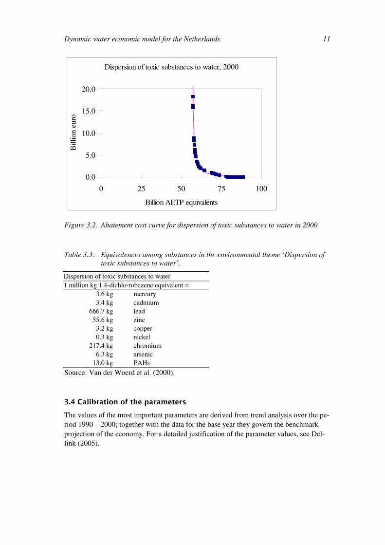
Figure 3.2 shows the total amount of abatement costs and emission reduction potential

for ‘dispersion of toxic substances to water’. Based on the information of individual

measures, we approximate the cost abatement curve in a CES structure that will be used

in the model calculations.8

8 An update of these curves, using improved information on abatement measures for specific

sectors, is envisaged as part of future research.


Dispersion of toxic substances to water, 2000

0.0

5.0

10.0

15.0

20.0

0 25 50 75 100

Billion AETP equivalents

Bil

lio

n e

uro

s

Figure 3.2. Abatement cost curve for dispersion of toxic substances to water in 2000.

Table 3.3: Equivalences among substances in the environmental theme ‘Dispersion of

toxic substances to water’.

Dispersion of toxic substances to water

1 million kg 1.4-dichlo-robezene equivalent =

3.6 kg mercury

3.4 kg cadmium

666.7 kg lead

55.6 kg zinc

3.2 kg copper

0.3 kg nickel

217.4 kg chromium

6.3 kg arsenic

13.0 kg PAHs

Source: Van der Woerd et al. (2000).

3.4 Calibration of the parameters

The values of the most important parameters are derived from trend analysis over the pe-

riod 1990 – 2000; together with the data for the base year they govern the benchmark

projection of the economy. For a detailed justification of the parameter values, see Del-

link (2005).


The growth rate of labour supply equals 2 percent; and a stable annual interest rate of 4%

is used.9 The steady-state relationship between investments and capital is used to calcu-

late a depreciation rate of 3 percent. The values for the substitution elasticities and the

nesting structure for the production functions, the utility function and the international

trade functions are taken from Gerlagh et al. (2002) and represent adaptation possibilities

for the medium term. The intertemporal elasticity of substitution has to be calibrated

only for the private households; the value equals 0.5.

The pollution-abatement-substitution (PAS) elasticities, benchmark price of the emission

permits and technical potential for pollution reduction are directly derived from the

abatement cost curves (Dellink, 2005). The growth rate of the technical potential for pol-

lution reduction is based on a comparison of the abatement cost curves for 1990 and

2000, using Hofkes et al. (2002) and Brouwer et al. (2007). The autonomous pollution

efficiency improvements are calibrated for each environmental theme separately using

the realised development of emission levels between 1995 and 2000; the ad-hoc assump-

tion is made that these effects of current policies will fade over time, leading to a stabili-

sation of benchmark emissions in the long run.10 The autonomous abatement efficiency

improvement is calibrated to 0.5 percent per year throughout the model horizon.

9 This interest rate is 1 percent point lower than in Dellink (2005), to reflect recent develop-

ments. 10

Pollution efficiency improvements reflect the impacts of other environmental policies, such

as the European Nitrate Directive (91/676/EC), Urban Waste Water Treatment Directive

(91/271/EC) amongst others.


4. Results

4.1 Benchmark development and policy scenarios

In the benchmark, the economy is assumed to be on a balanced growth path. Economic

activity increases with 2 percent per year, whereas the growth rates for emissions are de-

termined by the combination of the economic growth rate, and the assumed autonomous

pollution efficiency improvements.

The water quality requirements of the WFD are yet unknown, which makes it impossible

to calculate the exact consequences of the implementation of the WFD. Furthermore, the

dynamic AGE model requires standards for emissions for the environmental themes

rather than water quality standards, and the water quality requirements have to be trans-

lated into emission standards for water related substances. Therefore, we simulate the

economic consequences for different emission reduction scenarios ranging from 20 to 50

percent emission reduction from 2015 onwards with respect to emission levels in 2000.

The implementation of the WFD will be executed gradually (see Van der Veeren, 2005;

Brouwer, 2005) and we assume that the implementation will start effectively in 2008. In

addition, we compare these to results for scenarios with a derogation of the target until

2027 (see Van der Veeren, 2005, for a discussion of the appropriate emission reduction

scenarios). Given the assumed autonomous emission reduction over time in the DEAN-

W model, the required 50 percent emission reduction in 2015 is roughly equivalent to a

50 percent emission reduction compared to the benchmark. A derogated target of 50%

reduction implies a 20% reduction of emissions in 2015 compared to the benchmark.

0

100

200

300

400

500

600

700

800

2000 2005 2010 2015 2020 2025 2030

Gross Domestic Product

Net National Income

Figure 4.1. Development of GDP in the benchmark projection.


Figure 4.1 presents the benchmark development of GDP. Developments of emissions

and emission targets for the different scenarios are given in Figures 4.2 and 4.3 for Eu-

trophication and Dispersion of heavy metals to water, respectively.

0

2

4

6

8

10

12

14

2000 2005 2010 2015 2020 2025 2030 2035

mln

. P

-eq

uiv

ale

nts

.

Benchmark development 20 percent reduction in 2015 30 percent reduction in 2015

40 percent reduction in 2015 50 percent reduction in 2015 50 percent reduction in 2027

Figure 4.2. Development of emissions of eutrophying substances over time in different

scenarios.

0

20

40

60

80

100

120

140

2000 2005 2010 2015 2020 2025 2030 2035

mln

. to

xic

eq

uiv

ale

nts

.

Benchmark development 20 percent reduction in 2015 30 percent reduction in 2015

40 percent reduction in 2015 50 percent reduction in 2015 50 percent reduction in 2027

Figure 4.3. Development of emissions of dispersion of toxic substances to water over

time in different scenarios.


4.2 Attaining the reduction target by 2015

The main results of the environmental policy where the emissions for Eutrophication and

Dispersion simultaneously have to be reduced by 20 percent with respect to the emission

level of 2000 are represented in Table 4.1. Given the reduction in emissions between

2000 and 2015 as a result of existing policies (see Section 3.4), the target for Eutrophica-

tion is not strictly binding: benchmark emissions are below the target. Thus, no addi-

tional efforts are required for this theme (see the emission reduction in percentage

change compared to the benchmark projection in Table 3.3), when the required emission

reduction is limited to 20% below 2000 levels. For Dispersion to Water, the target is

binding: from 2015 onwards, emissions will have to be reduced almost 10 percent below

benchmark projection levels. As marginal abatement costs for small amounts of reduc-

tion are relatively cheap, these emission reductions can completely be achieved through

the implementation of low-cost technical measures. The macroeconomic results suggest

that these adjustments in the economy are virtually costless. This does not mean that

there are no substantial differences in terms of volume changes between the production

of economic sectors. While there is hardly any change for the Service sectors, Agricul-

ture suffers a 1.5% loss of production volume.

Table 4.1: Main results for a required 20% reduction in emissions

2010 2015 2020 2030

Macroeconomic results (%-change in volumes compared to benchmark projection)

GDP 0.0 0.0 0.0 0.0

NNI 0.0 0.0 0.0 0.0

Total private consumption 0.0 0.0 0.0 0.0

Total production 0.0 0.0 0.0 0.0

Capital investment 0.0 0.0 0.0 0.0

Sectoral results (%-change in volumes compared to benchmark projection)

Private consumption Agriculture -0.1 -0.1 -0.1 -0.1

Private consumption Industry 0.0 0.0 0.0 0.0

Private consumption Services 0.0 0.0 0.0 0.0

Sectoral production Agriculture -1.4 -1.5 -1.5 -1.5

Sectoral production Industry -0.1 -0.1 -0.1 -0.1

Sectoral production Services 0.0 0.0 0.0 0.0

Sectoral production Abatement services 24.9 28.0 28.0 28.0

Environmental results (%-change in volumes compared to benchmark projection)

Emissions Eutrophication 0.0 0.0 0.0 0.0

Emissions Dispersion to Water -3.6 -9.5 -9.5 -9.5

Prices of main variables (constant 2000 prices)

Wage rate index (benchmark index = 1) 1.0 1.0 1.0 1.0

Exchange rate index (benchmark index = 1) 1.0 1.0 1.0 1.0

Price of abatement services (bm. index = 1) 1.0 0.9 0.9 0.9

Price Eutrophication permits (bm. index = 1) 1.5 1.7 1.9 2.3

Price Dispersion permits (bm. index = 1) 1.5 2.1 2.3 2.8


The prices of emission permits for Eutrophication and Dispersion to Water both increase

over time, but remain at a low level. Though the required percentage reduction in emis-

sions remains constant from 2015 onwards, the permit price increases over time reflect-

ing the autonomous efficiency improvements in the benchmark11, that induce compensat-

ing price increases; this effect carries over from the benchmark to the counterfactual

simulations.

Note, however, that there is still uncertainty whether the scenario of 20 percent emission

reduction compared to the emission in the year 2000 is sufficient to meet the water qual-

ity targets of the WFD in 2015. Stone et al. (forthcoming) calculate the water quality im-

pacts of the different emission reduction scenarios calculated with DEAN-W.

Table 4.2 shows the main results for the more stringent policy where emission reductions

of 50 percent (compared to emission levels in 2000) are required. As the stringency of

the policy increases, the impacts become visible at the macro-economic level: GDP and

NNI levels are decreasing. In the short run, the economic growth rate is reduced to below

the benchmark level of 2 percent, the effect is strongest in 2015, where the growth rate

equals 1.6 percent. But after 2015 the adjustment process stabilizes and the growth rate

returns to 2 percent annually. The level of GDP and NNI is, however, permanently

lower. For both themes, the more stringent target is binding, and from 2015 onwards

emissions have to be reduced below benchmark projection levels by 36 and 43 percent,

respectively. This stimulates production in the Abatement services sector. Note that most

of the results for the years 2020 and 2030 are similar to the results for the year 2015 due

to the fact that DEAN-W assumes a balanced growth path. As a consequence, the emis-

sions stabilize after the WFD target is reached in 2015.

Not surprisingly, the Agricultural sector substantially reduces its production levels, as

this sector is the largest emitter of eutrophying substances and one of the largest emitters

of toxic substances. Production levels of the industrial sectors decrease by around 4 per-

cent. Thus, a shift in production from agriculture and industry towards the emission ex-

tensive services sector is induced. Aggregate production levels are also negative af-

fected, but the reduction in consumption is limited, mainly due to lower investments.

In the short run, consumers anticipate on the environmental policy by changing their sav-

ings/consumption decision. Households increase their consumption in the short run at the

expense of savings, as this has a positive effect on welfare, while accepting a lower

growth rate of the economy (as the lower savings translate into lower investments and

consequently into a lower growth rate of capital) and thus lower consumption levels in

the long run. This reduction in the growth rate of the economy is one part of the optimal

mix of reactions to the stringent environmental policy, together with expenditures on

abatement and a restructuring of the economy. As consumers optimize their intertempo-

ral utility function, this mix is the cost-effective response to the new policy.

11 These efficiency improvements imply that the volume of inputs of emission permits in the

benchmark reduces over time; this is compensated by a simultaneous increase in benchmark

prices, such that the value of these inputs is in line with the common growth rate of the

benchmark projection, i.e. the value share of all inputs remains constant in the benchmark

projection.


Table 4.2. Main results for a required 50% reduction in emissions

2010 2015 2020 2030


GDP -0.2 -0.7 -0.8 -0.8

NNI 0.0 -0.8 -0.8 -0.8

Total private consumption 0.2 -0.1 -0.2 -0.2

Total production -0.2 -1.4 -1.5 -1.5

Capital investment -1.0 -0.7 -0.7 -0.7


Private consumption Agriculture 0.0 -3.0 -3.0 -3.0

Private consumption Industry 0.1 -0.8 -0.8 -0.9







Emissions Eutrophication -13.6 -36.4 -36.4 -36.4








-1.0%

-0.9%

-0.8%

-0.7%

-0.6%

-0.5%

-0.4%

-0.3%

-0.2%

-0.1%

0.0%

2000 2005 2010 2015 2020 2025 2030

20% reduction in 2015





Figure 4.4. Percentage change in GDP – development over time


Figure 4.4 shows the development of the percentage change in GDP over time in the dif-

ferent scenarios. The figure reflects that limited emission reduction targets can be met at

little or no macroeconomic costs, but the economic costs of the policy increases more

than proportionately with the stringency of the policy. This is trivial: first, the cheapest

options to reduce emissions are implemented, and further reductions will have to be real-

ized through more costly adjustments. The costs of economic adjustments also increase

more than proportionately with stringency, as consumers prefer to stay as close as possi-

ble to the original consumption bundle.

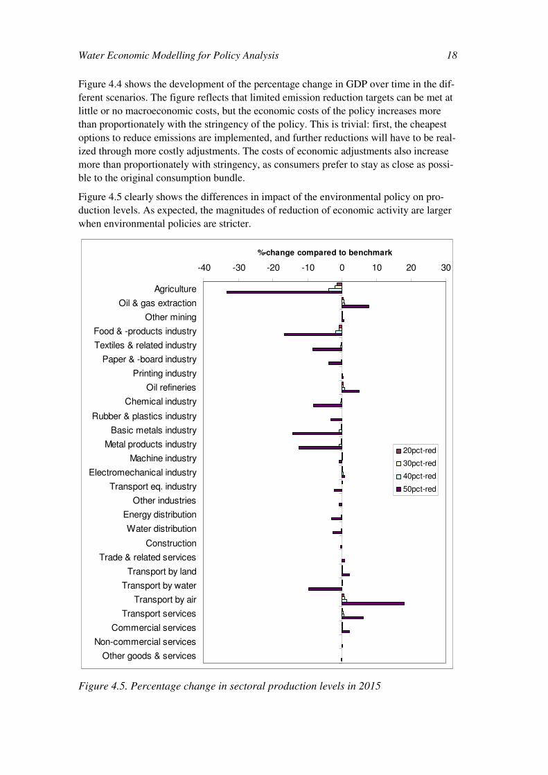
Figure 4.5 clearly shows the differences in impact of the environmental policy on pro-

duction levels. As expected, the magnitudes of reduction of economic activity are larger

when environmental policies are stricter.

-40 -30 -20 -10 0 10 20 30

Agriculture

Oil & gas extraction

Other mining

Food & -products industry

Textiles & related industry

Paper & -board industry

Printing industry

Oil refineries

Chemical industry

Rubber & plastics industry

Basic metals industry

Metal products industry

Machine industry

Electromechanical industry

Transport eq. industry

Other industries

Energy distribution

Water distribution

Construction

Trade & related services

Transport by land

Transport by water

Transport by air

Transport services

Commercial services

Non-commercial services

Other goods & services

%-change compared to benchmark

20pct-red

30pct-red

40pct-red

50pct-red

Figure 4.5. Percentage change in sectoral production levels in 2015


In addition, Figure 4.4 shows that the impacts increase more than proportional with the

emission reduction scenarios ranging from 20 to 50 percent. The same picture emerges

from Figure 4.5 for the individual industries. For most sectors the impacts for the 50 per-

cent emission reduction scenario are more than proportionally larger than the impacts for

the 20 percent scenario. Note that this holds for sectors that suffer from the stricter emis-

sion reduction scenarios as well as for those that benefit. The main reason for this dis-

proportional impact of the emission reduction scenarios is the increasing marginal costs

of pollution abatement and the increase in restructuring of the economy.

This also means that the sectors that can benefit from the new policy, including not only

the Abatement sector (cf. Tables 4.1 and 4.2), but also for example Transport by Air, are

best served by a stringent policy (see Figure 4.5). The positive effect on Transport by Air

can be explained by comparing the emission levels of the different transport modes in

Table 3.2: there are no toxic emissions attributed to this sector, whereas the other trans-

port modes have substantial emissions.12 This illustrates that the economic impacts of

environmental policy can best be regarded as a reallocation of available resources, rather

than as a shrink of the economy. Thus, the sectoral impacts are much larger than the

macroeconomic results suggest. Clearly, when these water policies are embedded in a

wider range of environmental policies, the sectoral changes will be different, as different

environmental themes have very different emission patterns over the sectors. Dellink

(2005) investigates these interactions between different environmental problems in de-

tail. Thus, the result that Agriculture will be most severely affected should be regarded in

the context of a water policy only. Furthermore, a more detailed modeling of the agricul-

tural subsectors may show substantial differences between the subsectors.

12 This is an artefact of the way Statistics Netherlands attributes emissions: only emissions of air-

planes when landing and taking off are accounted for as Dutch emissions; in-flight emissions

are not attributed to the Dutch economy.


4.3 Derogation of reduction targets to 2027

Table 4.3. Main results for a derogated required 50% reduction in emissions

2010 2015 2020 2030


GDP -0.1 -0.2 -0.3 -0.8

NNI 0.0 -0.1 -0.1 -0.8

Total private consumption 0.1 0.1 0.1 -0.2

Total production -0.1 -0.2 -0.3 -1.5

Capital investment -0.5 -0.7 -1.0 -0.7


Private consumption Agriculture -0.1 -0.1 -0.1 -3.0

Private consumption Industry 0.1 0.0 0.0 -0.9







Emissions Eutrophication -5.5 -14.6 -23.7 -36.4








In the simulations presented above, the reduction target is introduced gradually and is

fully met by 2015. The Water Framework Directive does, under special circumstances,

allow for a derogation of these targets to 2027. This delayed target is simulated assuming

that the gradual adjustment process will start immediately, but is prolonged until 2027,

when the targets are fully met. The main results for this scenario are presented in Table

4.3. Obviously, this affects the economy between 2010 and 2027, but once the emission

reduction targets are fully implemented, the impacts are comparable to the scenario with

targets for 2015. Thus, it can be concluded that the derogation has only a temporary ef-

fect on the economy.

Figure 4.6 shows how the permit price for Dispersion to Water increases when the envi-

ronmental policy is implemented. These results confirm the discussion above. Notable is

that the derogation of the policy target has no impact on the price of dispersion permits

in the long run: these are solely determined by the strictness of the long-run policy.


0

50

100

150

200

250

300

350

400

2000 2005 2010 2015 2020 2025 2030






Figure 4.6. Permit price of Dispersion to Water – development over time

4.4 Decomposition of direct and indirect costs

The DEAN-W model describes the costs of the policies primarily in terms of changes in

GDP, NNI and sectoral changes in production and consumption levels. These sectoral

and macro-economic changes are the combined effect of direct and indirect effects. In a

CGE setting, the division between direct and indirect costs is less relevant than in partial

analyses, where only certain costs can be assessed, while others are ignored. Nonethe-

less, our results can also be expressed in terms of direct and indirect costs by calculating

sectors changes in generated value added; these value added changes add up to the

change in national product. The direct sectoral costs include expenditures by the sector

on abatement and on emission permits. The indirect costs (and benefits) include reduced

tax payments (as by assumption the permit revenues are redistributed by lowering exist-

ing tax levels), changes in production structure and changes in production volume. Table

4.4 shows the decomposition of costs for the 50 percent reduction scenario in 2015,13

where production sectors are aggregated into three broad categories.14 The column

‘Cons.’ encompasses costs to the private households and changes in value added gener-

ated through investments.

The total costs are evaluated at 3.7 billion Euro, or 0.7 percent of the GDP in the bench-

mark projection (cf. Table 4.2). The expenditures on emission permits and the associated

13 Since we are uncertain about the water quality impacts of emission reduction scenarios and

since the WFD targets for water quality are yet unknown, we choose the most conservative

scenario to be the most likely scenario to meet the WFD requirements of good water quality

status in all surface water in the Netherlands. 14

Obviously, the differences between individual sectors within these three broad categories are

substantial. A more detailed analysis of direct and indirect costs is presented in Dellink

(2008).


tax reduction do not have any macro-economic impact: these are merely a financial re-

distribution from the polluting sectors to the government and from the government to the

tax payers, respectively. For the government these scenarios are budget neutral. It is

striking to see that at the macro-economic level the indirect costs are much larger than

the direct costs. This can partially be explained by the concentration of emissions in rela-

tively few number of sectors: rather than investing large amounts in abatement, it may be

less costly to accept lower production levels in these few sectors, especially Agriculture,

and reduce emissions in that way. It should be noted that the CGE framework assumes

that production factors that become available by reducing production in one sector can

be usefully employed in other sectors. Thus, the macro-economic costs comprise of the

net effect of lower value added in the “dirty” sector plus higher value added in the other

“cleaner” sectors. Again, this shows the importance of adopting a framework that can in-

corporate indirect effects in a consistent manner.

The sectoral direct costs reflect the shares of the different sectors in emissions (cf. Table

3.2): the higher the emissions, the more the sector needs to spend on abatement and buy-

ing permits. As Industry is a much larger sector than Agriculture, the largest absolute

costs are borne by Industry; the relative burden on Agriculture is however much higher.

The sectoral indirect costs, without the tax reduction, are negative for Agriculture and

Industry, and positive for Services. This reflects the natural tendency that the optimal re-

action to changes in policy contain a mechanism of dampening extreme effects in order

to smoothen the adjustments and minimize the impact of the policy on consumption pat-

terns.15 At the level of individual sectors, the effects are more pronounced. For instance,

the Food and food-products industry is confronted with the decline in Agriculture and

this causes substantial indirect costs in this industry (almost 1.5 billion Euro). Note that

since the total indirect benefits for the industrial sector are 1.2 billion Euro, the sum of

indirect benefits of the other industrial sub-sectors amount to 2.8 billion Euro). Substan-

tial indirect costs are also borne by the Non-commercial services; the main reason for

this is that substitution possibilities between production inputs are estimated to be much

smaller than in other sectors, due to the specific nature of many of the services produced

by this sector. Thus, this sector cannot respond as flexible to changes in relative prices as

other sectors.

The total costs reported for consumers contains several effects. First, households have to

invest in abatement and buy emission permits, as they are one of the major sources of

emissions for both environmental themes. Together, these account for 4.7 billion Euro.

Secondly, households benefit from the lower taxes, especially from the lower VAT

(more than 3 billion Euro), and adjusting consumption patterns as a response to changes

in relative prices of consumer goods also increases their income with more than 3 billion

Euro. In total, the private households have total net benefits of around 1.6 billion Euro.

Thirdly, investment levels decrease, and hence the value added generated from invest-

ment decreases substantially; this amounts to indirect costs of almost 2.5 billion Euro.

These effects counteract each other, and hence the total costs as reported in Table 4.4 are

relatively low. Finally, the changes for the government comprise purely of a redistribu-

15 Note that in DEAN-W, initial consumption are assumed to be optimal and thus any forced

change is considered to be detrimental to welfare.


tion effect: the endogenous adjustment of existing tax levels ensures that provision of

public goods remains constant throughout all simulations, and hence the different cost

components exactly cancel each other out.

Table 4.4. Direct and indirect costs in 2015 (mln. Euro) for a required 50% reduction in

emissions

Agric. Industry Ser-

vices

Abat

sector

Invest-

ment

Cons. Gov’t Total

Abatement costs Eutrophica-

tion

1 4 0 15 0 20

Dispersion 40 80 15 100 0 235

Eutrophica-

tion

35 16 0 51 -102 0Tradable emission

permits

Dispersion 2,390 3,802 703 4,558 -11,453 0

Tax reduction -126 -1,667 -6,145 -2,216 -3,100 13,254 0

Other indirect costs -243 -1,240 5,294 -152 4,686 -3,208 -1,699 3,438

Total costs 2,097 994 -132 -152 2,470 -1,585 0 3,692

Remark: A negative number means benefits, while a positive number means costs.


5. Concluding remarks

At low levels of environmental policy, say a 20 percent reduction in eutrophying emis-

sions and toxic substances dispersed to water compared to the historical levels in 2000,

there are opportunities for the economic agents to adjust to the new circumstances at

relatively low costs. Part of the emission reductions are expected to be achieved at zero

costs, as existing policies have already induced a partial decoupling of economic activity

and emissions. Furthermore, relatively cheap technical measures can be implemented to

reduce emissions, and the macroeconomic impacts of the policy remain very limited. At

more stringent levels of policy the low-cost possibilities to adjust are exhausted. Then,

an optimal mix arises from the trade-off between the implementation of technical meas-

ures, a restructuring of the economy and a temporary slowdown of economic growth (i.e.

increasing short-term consumption at the expense of savings).

Since we are uncertain about the water quality impacts of emission reduction scenarios

and since the WFD targets for water quality are yet unknown, we also calculated more

conservative scenarios to meet the WFD requirements of good water quality status in all

surface water in the Netherlands. Especially in the 50 percent emission reduction scenar-

ios, the economic impacts of the implementation of the WFD increase more than propor-

tional in comparison with the increase of the stringency of the emission reduction target.

The main reason is that the marginal costs of abating pollution increase more than pro-

portional when the emission reduction target are set at 50 percent; simply put, the cheap-

est adjustment options are implemented first, and the more stringent the policy becomes,

the more polluters have to resort to costly abatement measures or economic restructur-

ing. Especially emission intensive sectors such as Agriculture and a number of the Indus-

trial sectors suffer from more stringent emission reduction scenarios. On the other hand,

a few sectors (Air transport, for instance) benefit from the emission reduction. In fact,

these sectors have more than proportional increases in benefits when the emission reduc-

tion targets increase.

The direct and indirect economic costs of the WFD policy can be attributed to different

sectors by examining changes in value added, and the direct costs can also be attributed

to the two environmental themes by comparing emission permit prices and abatement

expenditures. The results show that the direct and indirect costs differ widely at the level

of individual economic sectors, while at the macro-economic level this distinction is ir-

relevant. In the case of a 50 percent emission reduction scenario, Agriculture has large

direct cost and small indirect benefits. The services sectors have benefits (primarily in

the form of tax reductions), which overcompensate the other direct and indirect costs.

This emission reduction scenario induces a restructuring of the economy from Agricul-

ture and Industry towards the Service sector. Consumers (households) face high costs for

the purchase of emission permits but are compensated by large tax reductions. For the

government, the implementation is budget neutral. Note that these effects are the effect

of a water policy only. When the water policies are embedded into a larger environ-

mental policy setting, which include other major environmental problems such as cli-

mate change and local air pollution, the sectoral results may differ substantially due to


interaction effects between the different policies (just as the two environmental themes

investigated here interact).

Note that the DEAN-W is applied to long-term or mid-term analysis, so that short-run

economic fluctuations (business cycle effects) are ignored. Moreover, the model assumes

that the levels of emission are constant after the WFD target is reached.

If we compare the results of DEAN-W and the static AGE model in Brouwer et al.

(2007), the decline in Net National Income seems to be much lower in the dynamic

model than in the static model. As the dynamic model predicts a 0.8 percent loss in NNI

compared to the benchmark in 2015, the static model predicts a 10 percent loss in NNI.

Apart from differences caused by the different data sources,16 the dynamic aspects of

autonomous emission efficiency and developments in the abatement cost curves are ig-

nored in the static model results. Similar differences between the dynamic and static

model (both calibrated to 1990) in the evaluation of a wide range of environmental prob-

lems are found in Dellink (2005), who analyses the differences in detail.

There are some obvious areas for improvement of our analysis. First, the balanced

growth path assumed in the model is relatively simple, and disregards structural changes

in preferences and the structure of the economy. It is expected that most service (sub-)

sectors in the economy show a more than proportional growth rate, while the reverse is

the case in the agricultural sector. Secondly, the model represents a national economy,

where the environmental issues at stake are largely regional. Regionalising the model

will improve the link between economic activity and water pollution, as the activities can

be closely linked to specific water bodies. This comes at a cost, however, that a lower

geographical scale of analysis will complicate the description of economic interactions.

At the national level, relevant data exists on how different sectors interact, but at the re-

gional level, serious data problems arise. This topic is dealt with in Linderhof and

Reinhard (2007). Thirdly, although it is possible to softlink the national results with

more detailed models at the scale of individual river basins, such as the WFD Explorer

model constructed by WL Delft for surface water quality in the Netherlands, a more di-

rect link would improve the analysis. Preliminary results for such a softlink are available

in Stone et al. (2007), which also discusses opportunities and pitfalls for an enhanced in-

tegration of the economic and hydrologic models. Fourthly, the representation of water

quality in the model is highly stylized and deserves a more disaggregated approach. A

first step is to consider individual substances instead of environmental themes, although

we might run into problems with the data availability of the Pollution-Abatement curves.

Finally, the abatement cost functions used can be specified for individual sectors when

the appropriate data are available. While it might be infeasible to extent the model in all

directions simultaneously, it is the ambition of the WEMPA project to provide further

insights into many of these issues in order to come to the best available assessment of the

economic impacts of the WFD.

16 DEAN-W uses updated emission and economic data for the year 2000 in comparison with

Brouwer et al. (2007).


References

Barro, R.J. and X. Sala-i-Martin (1995). Economic Growth. New York. McGraw-Hill.

Brouwer, R. (2005). Toekomstige beleidsvragen en hun implicaties voor de ontwikkeling van een

integraal water-en-economie model (in Dutch). Water Economic Modelling for Policy Ana-

lysis report-01. Institute for Environmental Studies, Vrije Universiteit, Amsterdam. 19 pp.

Brouwer, R., Hofkes, M. and Linderhof, V. (2008). General equilibrium modelling of the direct

and indirect economic impacts of water quality improvements in the Netherlands at national

and river basin scale. Special issue Ecological Economics Integrated Hydro-Economic Mod-

elling: Approaches, Key Issues and Future Research Directions. In press.

Dellink, R.B. (2005). Modelling the costs of environmental policy: a dynamic applied general

equilibrium assessment. Cheltenham: Edward Elgar.

Dellink, R.B. (2008). Wat zijn de directe en indirecte sectorale kosten van implementatie van de

Kader Richtlijn Water in Nederland? forthcoming as WEMPA Working Paper. Institute for

Environmental Studies, Vrije Universiteit, Amsterdam.

Dellink, R.B., R. Gerlagh, M.W. Hofkes and L. Brander (2001). Calibration of an applied gen-

eral equilibrium model for the Netherlands in 1990. IVM report W-01/17. Institute for Envi-

ronmental Studies, Vrije Universiteit, Amsterdam.

Dellink, R.B. and E.C. van Ierland (2005). Pollution abatement in the Netherlands: a dynamic

applied general equilibrium assessment. Journal of Policy Modelling 28, 207-221.

Dellink, R. and V. Linderhof (2006). Dynamic AGE model for water economics in the Nether-

lands (DEAN-WEMPA): first results. WEMPA Working Paper 04. Institute for Environmen-

tal Studies, Vrije Universiteit, Amsterdam.

Dellink, R. and V. Linderhof (2007). Dynamic AGE model for water economics in the Nether-

lands (DEAN-WEMPA): an update. WEMPA Working Paper 05. Institute for Environmental

Studies, Vrije Universiteit, Amsterdam.

Gerlagh, R., R.B. Dellink, M.W. Hofkes and H. Verbruggen (2002). A measure of Sustainable

National Income for the Netherlands. Ecological Economics 41, 157-174.

Hofkes, M.W., R. Gerlagh, W. Lise and H. Verbruggen (2002). Sustainable National Income: a

trend analysis for the Netherlands for 1990 – 1995. IVM report R-02/02. Institute for Envi-

ronmental Studies, Vrije Universiteit, Amsterdam.

Hofkes, M., Gerlagh, R. & Linderhof, V. (2004). Trend analysis of sustainable national income

for the Netherlands, 1990-2000. IVM report (R04-02). Institute for Environmental Studies,

Vrije Universiteit Amsterdam, 62 pp.

Huijbregts M.A.J., U. Thissen, J.B. Guinée , T. Jager, D. Kalf, D. van de Meent, A.M.J. Ragas,

A. Wegener Sleeswijk, L. Reijnders (2000). Priority assessment of toxic substances in life

cycle assessment. Part I: Calculation of toxicity potentials for 181 substances with the nested

multi-media fate, exposure and effects model USES-LCA. Chemosphere 41, 541-573.

Hueting, R. (1996). Three persistent myths in the environmental debate. Ecological Economics

18, 81-88.

Linderhof, V., S. Reinhard, R. Brouwer and J. Icke (2008). Coherency of WEMPA models.

WEMPA report-09.

Reinhard, S. and V. Linderhof (2006). Inventory of economic models. Water Economic Model-

ling for Policy Analysis report-03. Institute for Environmental Studies, Vrije Universiteit,

Amsterdam. 49 pp.

Statistics Netherlands (2007). Milieurekeningen 2005, Voorburg.


Stone, K., R. Dellink., V. Linderhof., R. Brouwer and J. Icke (2008). De consequenties van de

Kaderrichtlijn Water (KRW) op de Nederlandse economie en waterkwaliteit: integratie van

economie en waterkwaliteit modellen op nationaal niveau. WEMPA report-06. Institute for

Environmental Studies, Vrije Universiteit, Amsterdam.

Van de Veeren, R. (2005). Development of policy scenarios and measures. Water Economic

Modelling for Policy Analysis report-04. Institute for Environmental Studies, Vrije Universi-

teit, Amsterdam. 31 pp.

Van der Woerd, F., E. Ruijgrok & R. Dellink (2000). Kosteneffectiviteit van verspreiding naar

water. IVM report E-00/01. Institute for Environmental Studies, Vrije Universiteit, Amster-

dam.

.


Publications from the project "Water Economic Modelling for Policy Analysis"

(see www.ivm.falw.vu.nl/watereconomics):

WEMPA report

Reportnumber Authors Title

WEMPA Report-01 Roy Brouwer Toekomstige beleidsvragen en hun implicaties voor de ontwik-

keling van een integraal water-en-economie model

WEMPA Report-02 Paul Baan

Aline te Linde

Inventory of water system models

WEMPA Report-03 Stijn Reinhard

Vincent Linderhof

Inventory of economic models

WEMPA Report-04 Rob van der Veeren Development of policy scenarios and measures

WEMPA report

Working paper Athors Title

WEMPA working paper-01 Paul Baan Households and recreation: use and value of water

WEMPA working paper-02 Paul Baan Emissiereductie RWZI's en Huishoudens

WEMPA working paper-03 Sjoerd Schenau Data availability for the WEMPA project

WEMPA working paper-04 Rob Dellink

Vincent Linderhof


Netherlands (DEAN-WEMPA): first results

WEMPA working paper-05 Rob Dellink

Vincent Linderhof


Netherlands (DEAN-WEMPA): an update

WEMPA working paper-06 Frans Oosterhuis Ervaringen met verhandelbare rechten in het water-

kwaliteitsbeleid van de Verenigde Staten

WEMPA working paper-07 Frans Oosterhuis Opportunities for the use of tradeable permits in

Dutch water quality policy

WEMPA working paper-08 Paul Baan Assessing the cost-effectiveness of pollution abate-

ment measures in communal wastewater treatment

plants

WEMPA working paper-09 Petra Hellegers Nico

Polman

Assessing the cost-effectiveness of pollution abate-

ment measures in agriculture

WEMPA working paper-10 Arnout van Soesbergen Assessing the cost-effectiveness of pollution abate-

ment measures in industry

Dynamic AGE model for water economics in the Netherlands ...€¦ · Dynamic AGE model for water...

Documents

Transcript of Dynamic AGE model for water economics in the Netherlands ...€¦ · Dynamic AGE model for water...