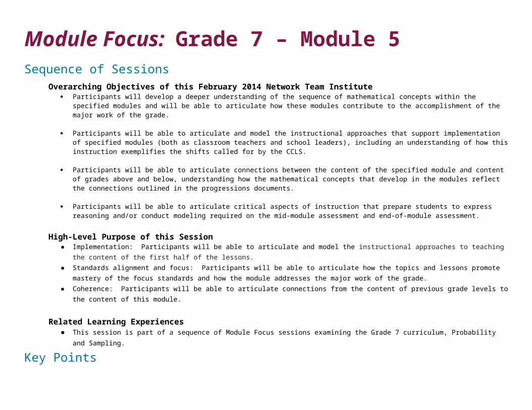
Module Focus: Grade 7 – Module 5 Sequence of Sessions

Overarching Objectives of this February 2014 Network Team Institute Participants will develop a deeper understanding of the sequence of mathematical concepts within the specified modules and will be able to articulate

how these modules contribute to the accomplishment of the major work of the grade.

Participants will be able to articulate and model the instructional approaches that support implementation of specified modules (both as classroom teachers and school leaders), including an understanding of how this instruction exemplifies the shifts called for by the CCLS.

Participants will be able to articulate connections between the content of the specified module and content of grades above and below, understanding how the mathematical concepts that develop in the modules reflect the connections outlined in the progressions documents.

Participants will be able to articulate critical aspects of instruction that prepare students to express reasoning and/or conduct modeling required on the mid-module assessment and end-of-module assessment.

High-Level Purpose of this Session● Implementation: Participants will be able to articulate and model the instructional approaches to teaching the content of the first half of the lessons.● Standards alignment and focus: Participants will be able to articulate how the topics and lessons promote mastery of the focus standards and how the

module addresses the major work of the grade.● Coherence: Participants will be able to articulate connections from the content of previous grade levels to the content of this module.

Related Learning Experiences● This session is part of a sequence of Module Focus sessions examining the Grade 7 curriculum, Probability and Sampling.

Key Points Probabilities can be estimated using simulation. The results of random samples are representative of a population. It is important to consider sampling variability when comparing two populations.

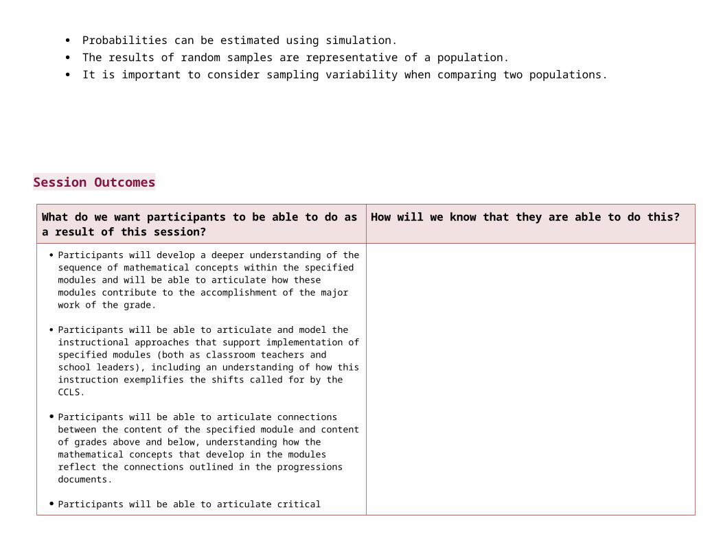
Session Outcomes

What do we want participants to be able to do as a result of this session?

How will we know that they are able to do this?

Participants will develop a deeper understanding of the sequence of mathematical concepts within the specified modules and will be able to articulate how these modules contribute to the accomplishment of the major work of the grade.

Participants will be able to articulate and model the instructional approaches that support implementation of specified modules (both as classroom teachers and school leaders), including an understanding of how this instruction exemplifies the shifts called for by the CCLS.

Participants will be able to articulate connections between the content of the specified module and content of grades above and below, understanding how the mathematical concepts that develop in the modules reflect the connections outlined in the progressions documents.

Participants will be able to articulate critical aspects of instruction that prepare students to express reasoning and/or conduct modeling required on the mid-module assessment and end-of-module assessment.

Session Overview

Section Time Overview Prepared Resources Facilitator Preparation

Introduction to Module

Concept Development

Module Review

Session Roadmap

Section: Grade 7 Module 5 Time: 180 minutes

[180 minutes] In this section, you will… Materials used include:

TimeSlide #

Slide #/ Pic of Slide Script/ Activity directions GROUP

1. Welcome! In this module focus session, we will examine Grade 7 – Module 5.

5 min 2.

6 min 3. Introduction to Grade 7 Module 5.

This module is divided into 4 topics. Overview each topic. Have participants turn to page 3-5 of teacher materials to see the specific standards.

Topic A introduces students to new terms, such as chance experiments and events. Students learn how to determine probabilities from equally likely outcomes as well as unequally likely outcomes. They will also learn to use graphical devices to determine probabilities.

Topic B introduces students to the difference between theoretical probability and estimated probability. Students will also use simulation to estimate probabilities.

Topic C introduces students to methods of selecting random samples, sampling variability, and estimating a population mean from a sample.

Topic D stresses the importance of sampling variablility in

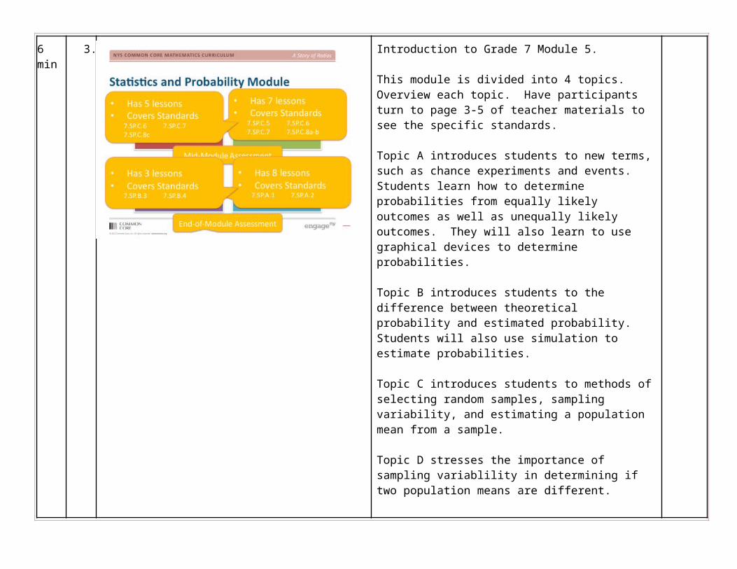
determining if two population means are different.

30 sec

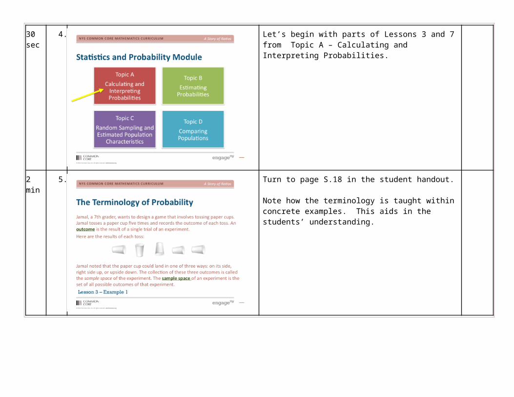
4. Let’s begin with parts of Lessons 3 and 7 from Topic A – Calculating and Interpreting Probabilities.

2 min 5. Turn to page S.18 in the student handout.

Note how the terminology is taught within concrete examples. This aids in the students’ understanding.

10 min

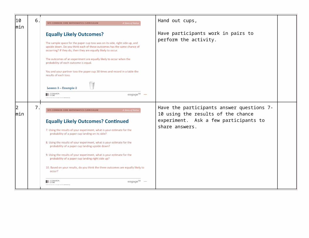
6. Hand out cups,

Have participants work in pairs to perform the activity.

2 min 7. Have the participants answer questions 7-10 using the results of the chance experiment. Ask a few participants to share answers.

5 min 8. Have participants make a prediction for questions 7-10 using 120 tosses.

Instead of tossing the cup 120 times, have 4 pairs combine their results. Determine the answers for 7-10.

Why do the predictions differ from the actual numbers? (In the long-run, the estimated probability approaches the actual (theoretical) probability.)

10 min

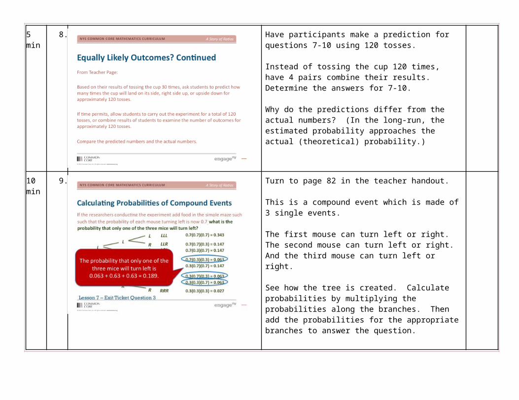
9. Turn to page 82 in the teacher handout.

This is a compound event which is made of 3 single events.

The first mouse can turn left or right. The second mouse can turn left or right. And the third mouse can turn left or right.

See how the tree is created. Calculate probabilities by multiplying the probabilities along the branches. Then add the probabilities for the appropriate branches to answer the question.

30 sec

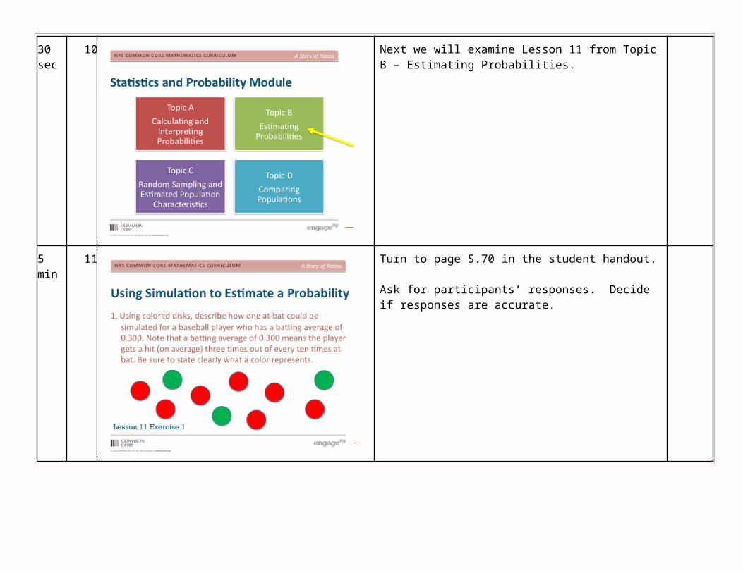
10. Next we will examine Lesson 11 from Topic B – Estimating Probabilities.

5 min 11. Turn to page S.70 in the student handout.

Ask for participants’ responses. Decide if responses are accurate.

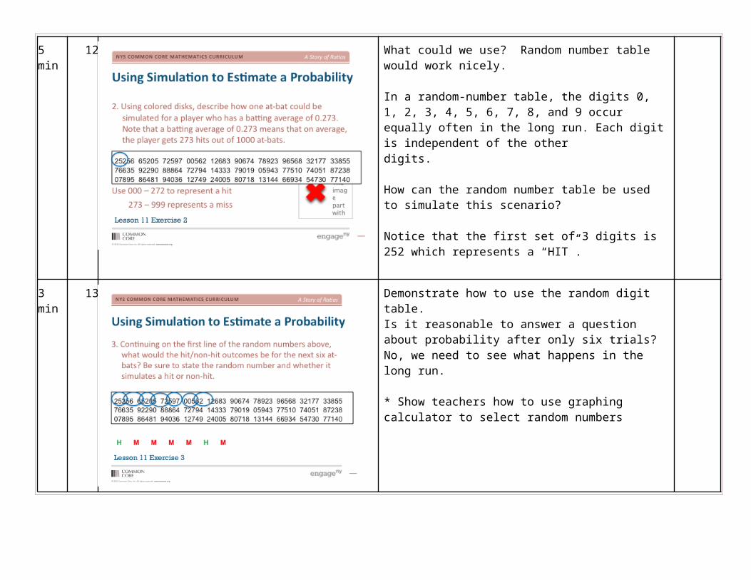
5 min 12. What could we use? Random number table would work nicely.

In a random-number table, the digits 0, 1, 2, 3, 4, 5, 6, 7, 8, and 9 occur equally often in the long run. Each digit is independent of the otherdigits.

How can the random number table be used to simulate this scenario?

Notice that the first set of 3 digits is 252 which represents a “HIT”.

3 min 13. Demonstrate how to use the random digit table.Is it reasonable to answer a question about probability after only six trials? No, we need to see what happens in the long run.

* Show teachers how to use graphing calculator to select random numbers

10 min

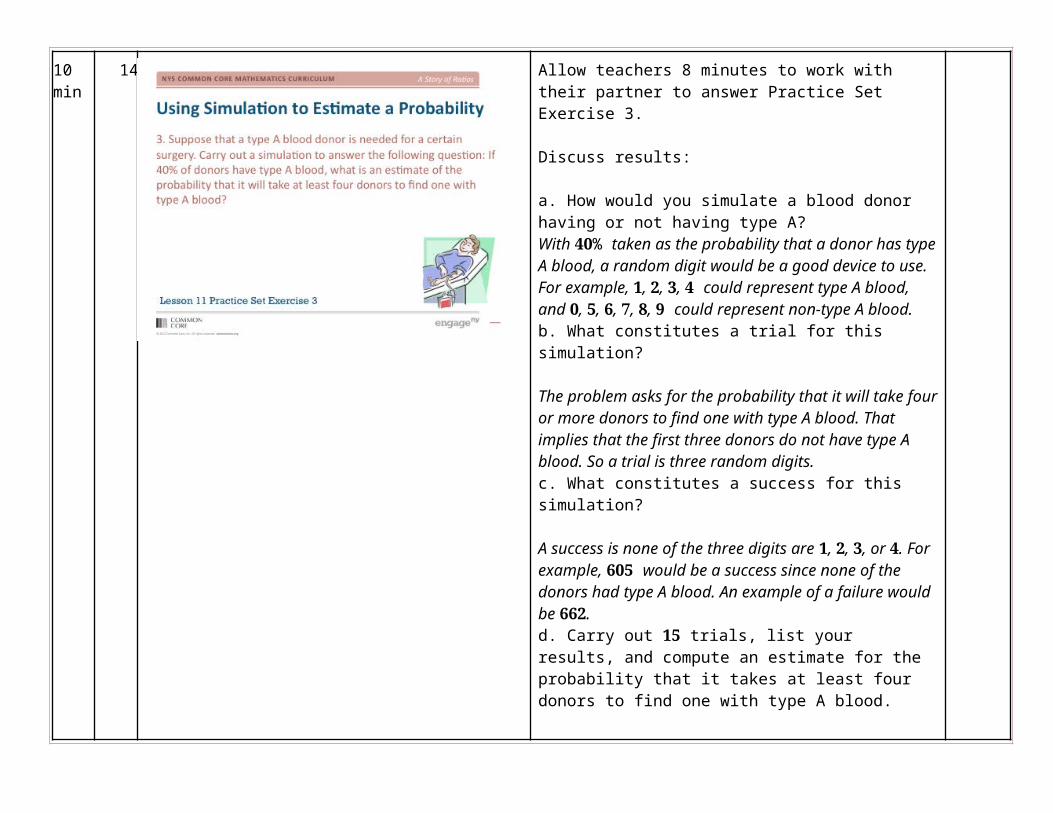
14. Allow teachers 8 minutes to work with their partner to answer Practice Set Exercise 3.

Discuss results:

a. How would you simulate a blood donor having or not having type A?With 𝟒𝟎% taken as the probability that a donor has type A blood, a random digit would be a good device to use. For example, 𝟏, 𝟐, 𝟑, 𝟒 could represent type A blood, and 𝟎, 𝟓, 𝟔, 𝟕, 𝟖, 𝟗 could represent non-type A blood.b. What constitutes a trial for this simulation?

The problem asks for the probability that it will take four or more donors to find one with type A blood. That implies that the first three donors do not have type A blood. So a trial is three random digits.c. What constitutes a success for this simulation?

A success is none of the three digits are 𝟏, 𝟐, 𝟑, or 𝟒. For example, 𝟔𝟎𝟓 would be a success since none of the donors had type A blood. An example of a failure would be 𝟔𝟔𝟐.d. Carry out 𝟏𝟓 trials, list your results, and compute an estimate for the probability that it takes at least four donors to find one with type A blood.

Students are to generate 𝟏𝟓 such trials, count the number of successes, and divide by 𝟏𝟓 to calculate their estimated probability of needing four or more donors to get one with type A blood.

Will all sets of partners have the same result? Why or why not?

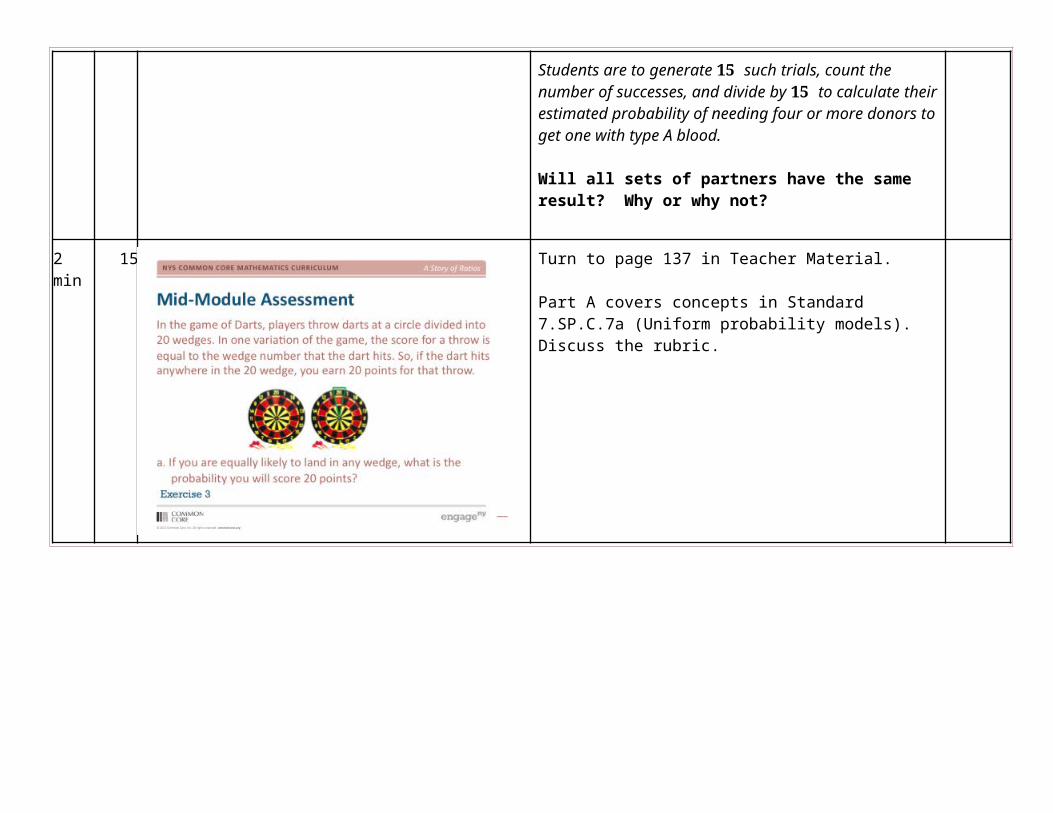
2 min 15. Turn to page 137 in Teacher Material.

Part A covers concepts in Standard 7.SP.C.7a (Uniform probability models). Discuss the rubric.

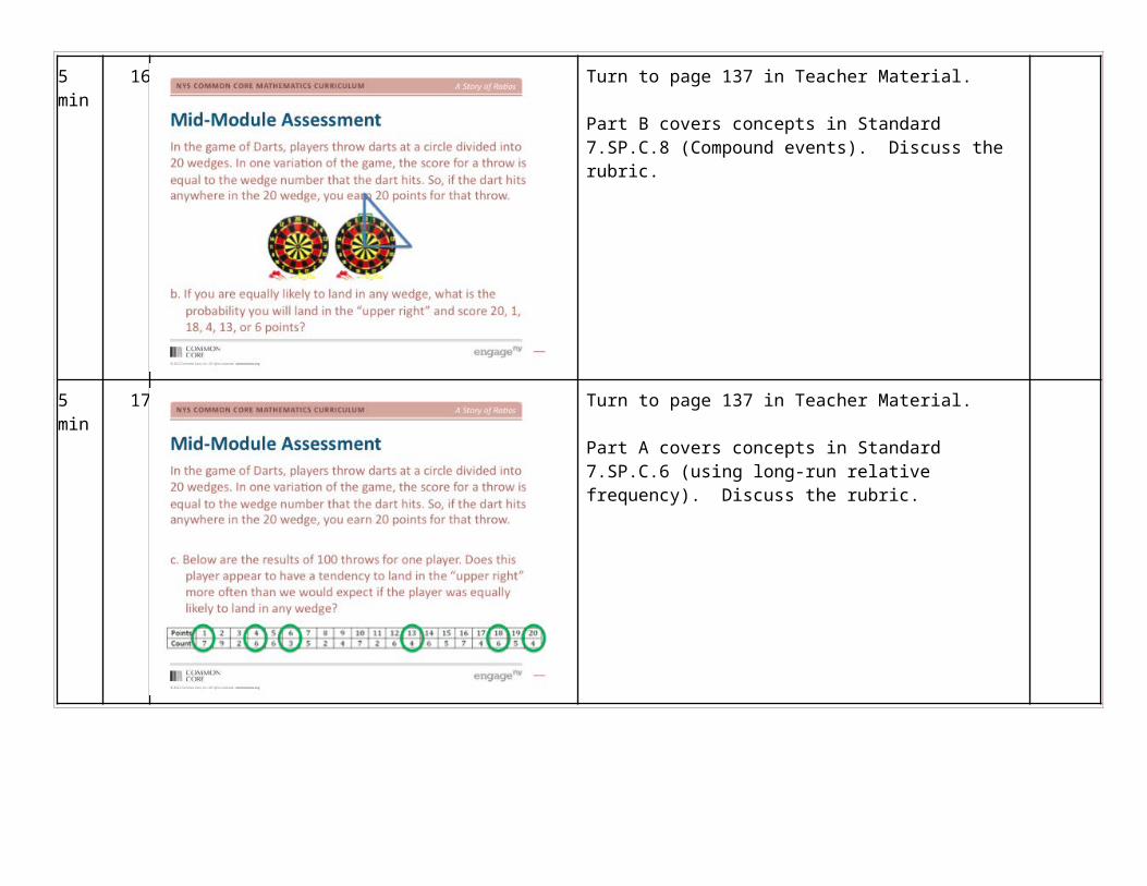
5 min 16. Turn to page 137 in Teacher Material.

Part B covers concepts in Standard 7.SP.C.8 (Compound events). Discuss the rubric.

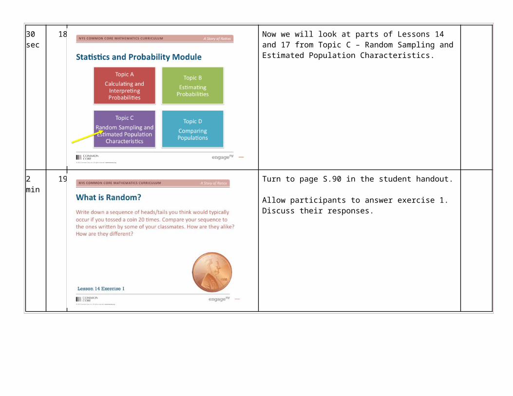
5 min 17. Turn to page 137 in Teacher Material.

Part A covers concepts in Standard 7.SP.C.6 (using long-run relative frequency). Discuss the rubric.

30 sec

18. Now we will look at parts of Lessons 14 and 17 from Topic C – Random Sampling and Estimated Population Characteristics.

2 min 19. Turn to page S.90 in the student handout.

Allow participants to answer exercise 1. Discuss their responses.

10 min

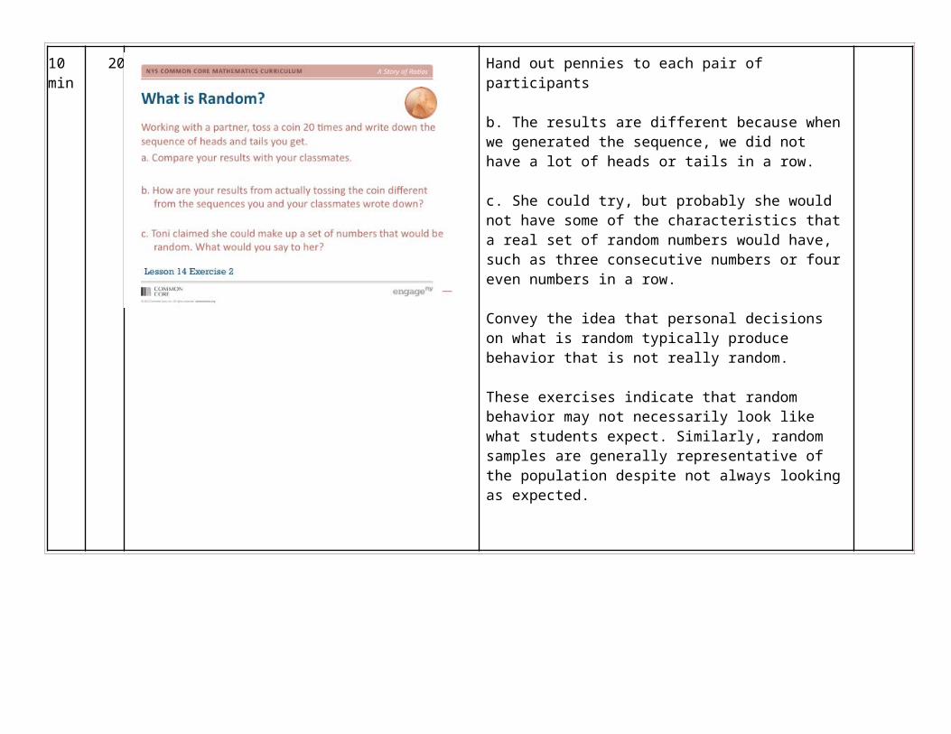
20. Hand out pennies to each pair of participants

b. The results are different because when we generated the sequence, we did not have a lot of heads or tails in a row.

c. She could try, but probably she would not have some of the characteristics that a real set of random numbers would have, such as three consecutive numbers or four even numbers in a row.

Convey the idea that personal decisions on what is random typically produce behavior that is not really random.

These exercises indicate that random behavior may not necessarily look like what students expect. Similarly, random samples are generally representative of the population despite not always looking as expected.

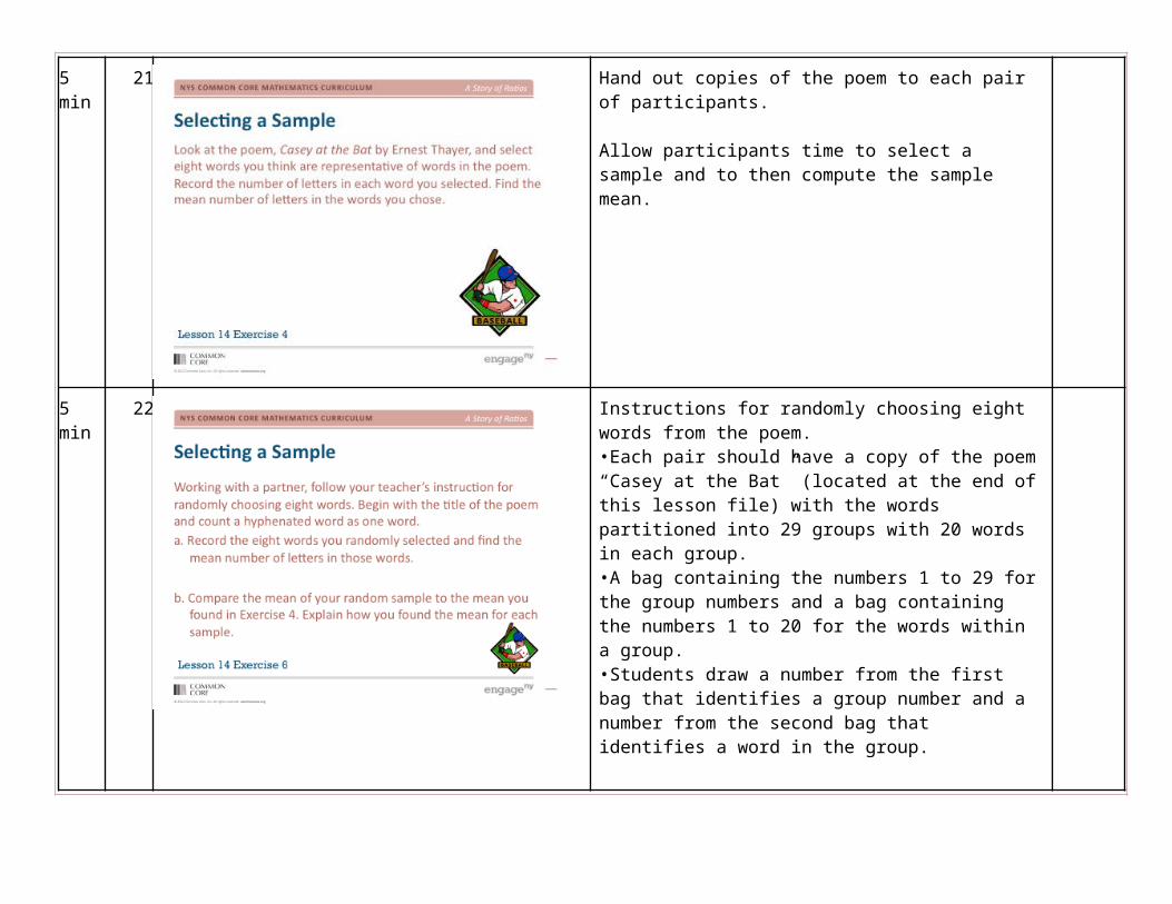
5 min 21. Hand out copies of the poem to each pair of participants.

Allow participants time to select a sample and to then compute the sample mean.

5 min 22. Instructions for randomly choosing eight words from the poem.•Each pair should have a copy of the poem “Casey at the Bat” (located at the end of this lesson file) with the words partitioned into 29 groups with 20 words in each group.•A bag containing the numbers 1 to 29 for the group numbers and a bag containing the numbers 1 to 20 for the words within a group.•Students draw a number from the first bag that identifies a group number and a number from the second bag that identifies a word in the group.

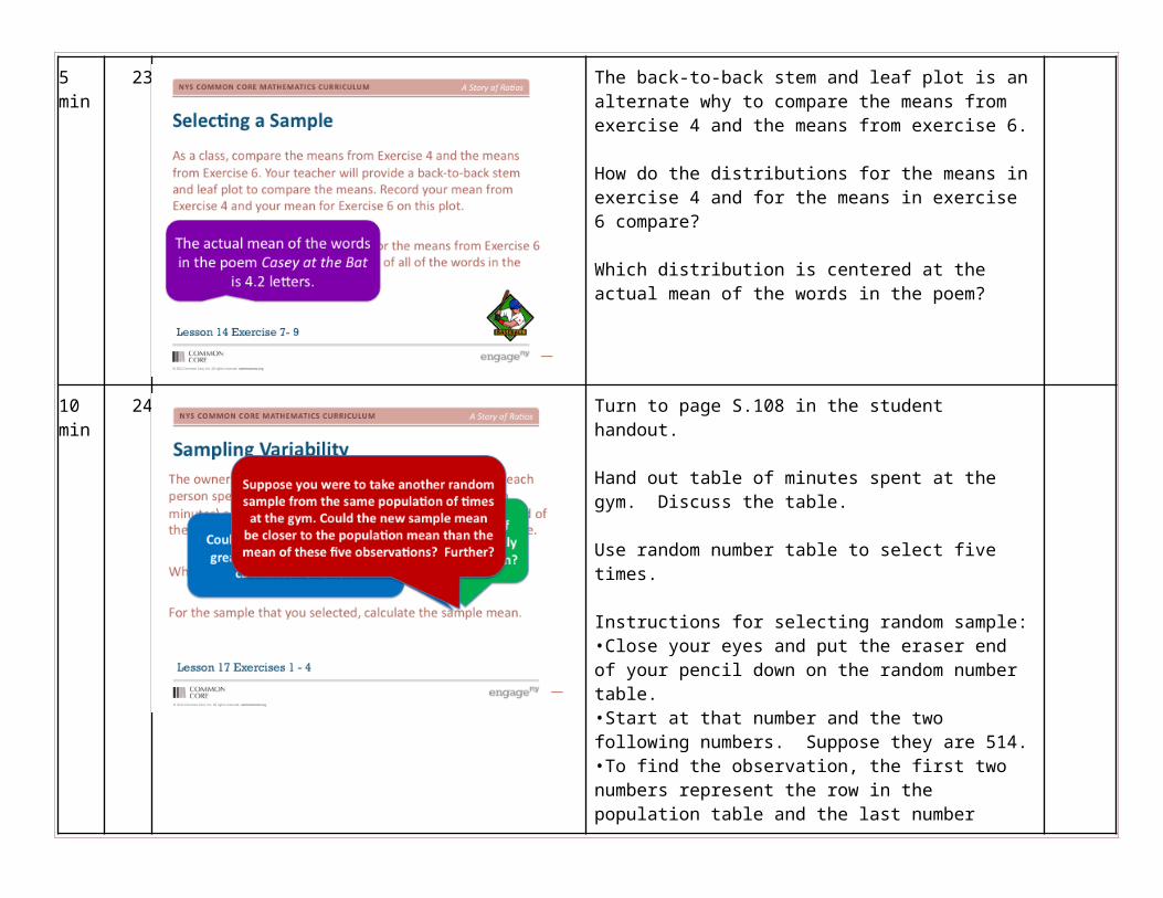
5 min 23. The back-to-back stem and leaf plot is an alternate why to compare the means from exercise 4 and the means from exercise 6.

How do the distributions for the means in exercise 4 and for the means in exercise 6 compare?

Which distribution is centered at the actual mean of the words in the poem?

10 min

24. Turn to page S.108 in the student handout.

Hand out table of minutes spent at the gym. Discuss the table.

Use random number table to select five times.

Instructions for selecting random sample:•Close your eyes and put the eraser end of your pencil down on the random number table.•Start at that number and the two following numbers. Suppose they are 514.•To find the observation, the first two numbers represent the row in the population table and the last number represents the column. Therefore, for the number 514, you would go to the 51st row and the 4th column.•Ignore numbers 800-999

Compute the sample mean, round to the nearest tenth.

1st & 2nd bubble - Make sure that students see that the value

of their sample mean is not likely to be exactly correct for the population mean. The population mean could be greater or less than the value of the sample mean.

3rd bubble - Make sure students understand that if they were to take a new random sample, the new sample mean is unlikely to be equal to the value of the sample mean of their first sample. It could be closer to or further from the population mean. Also note that if two sample means are the same – this does NOT mean that the samples are the same. It is possible that two different samples produce the same mean.

10 min

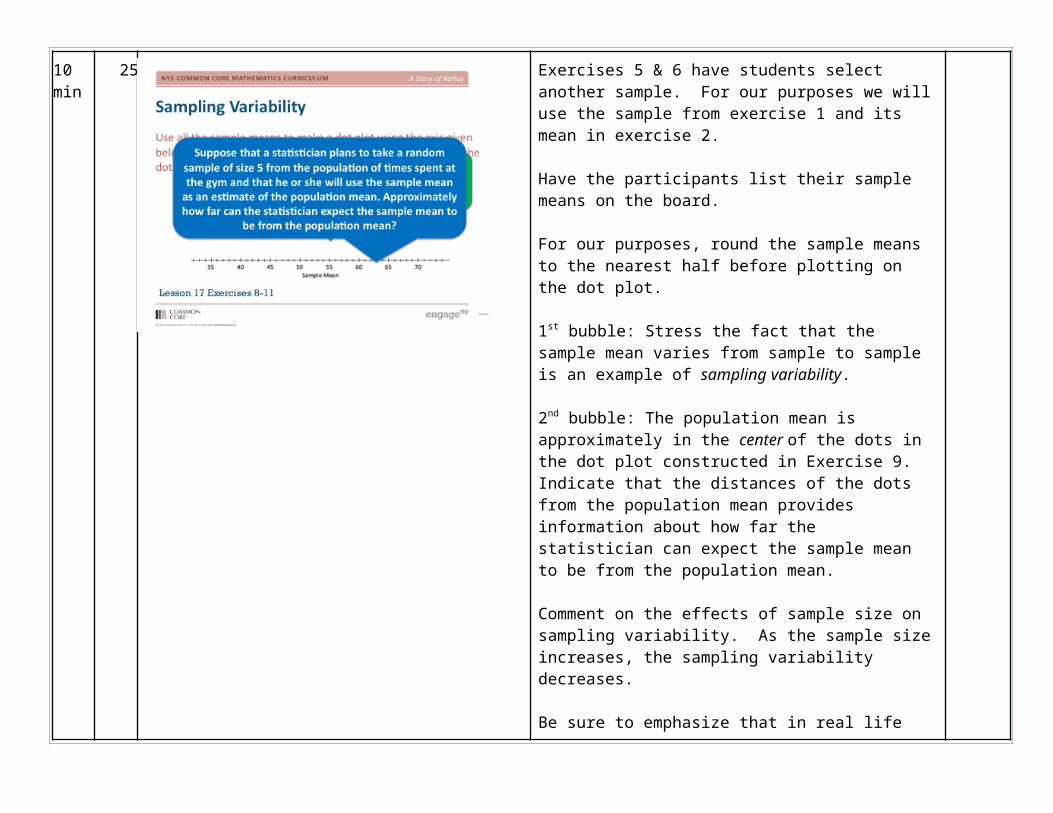
25. Exercises 5 & 6 have students select another sample. For our purposes we will use the sample from exercise 1 and its mean in exercise 2.

Have the participants list their sample means on the board.

For our purposes, round the sample means to the nearest half before plotting on the dot plot.

1st bubble: Stress the fact that the sample mean varies from sample to sample is an example of sampling variability.

2nd bubble: The population mean is approximately in the center of the dots in the dot plot constructed in Exercise 9. Indicate that the distances of the dots from the population mean provides information about how far the statistician can expect the sample mean to be from the population mean.

Comment on the effects of sample size on sampling variability. As the sample size increases, the sampling

variability decreases.

Be sure to emphasize that in real life ONLY one sample is selected and how sampling variability affects how close the sample mean is to the population mean.

30 sec

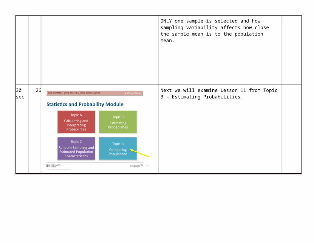
26. Next we will examine Lesson 11 from Topic B – Estimating Probabilities.

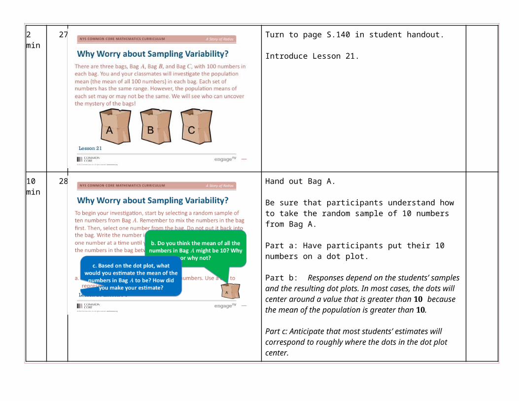
2 min 27. Turn to page S.140 in student handout.

Introduce Lesson 21.

10 min

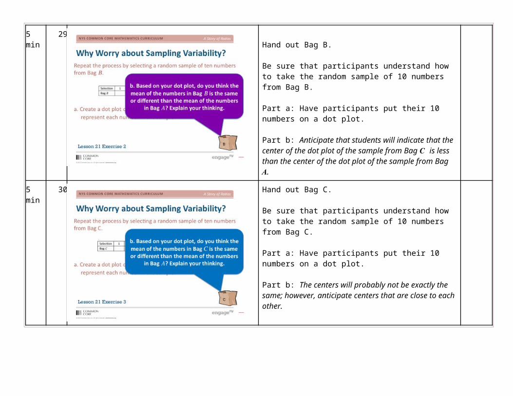
28. Hand out Bag A.

Be sure that participants understand how to take the random sample of 10 numbers from Bag A.

Part a: Have participants put their 10 numbers on a dot plot.

Part b: Responses depend on the students’ samples and the resulting dot plots. In most cases, the dots will center around a value that is greater than 𝟏𝟎 because the mean of the population is greater than 𝟏𝟎.

Part c: Anticipate that most students’ estimates will correspond to roughly where the dots in the dot plot center.

5 min 29.Hand out Bag B.

Be sure that participants understand how to take the random sample of 10 numbers from Bag B.

Part a: Have participants put their 10 numbers on a dot plot.

Part b: Anticipate that students will indicate that the center of the dot plot of the sample from Bag 𝑪 is less than the center of the dot plot of the sample from Bag 𝑨.

5 min 30. Hand out Bag C.

Be sure that participants understand how to take the random sample of 10 numbers from Bag C.

Part a: Have participants put their 10 numbers on a dot plot.

Part b: The centers will probably not be exactly the same; however, anticipate centers that are close to each other.

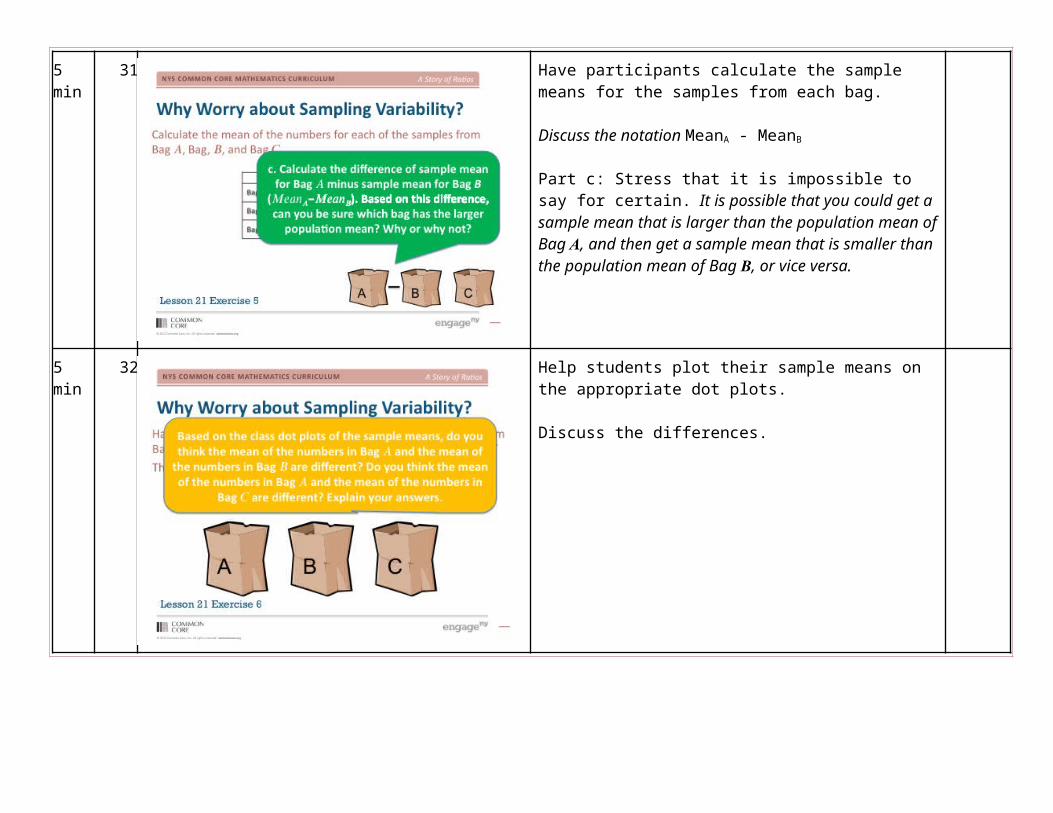
5 min 31. Have participants calculate the sample means for the samples from each bag.

Discuss the notation MeanA - MeanB

Part c: Stress that it is impossible to say for certain. It is possible that you could get a sample mean that is larger than the population mean of Bag 𝑨, and then get a sample mean that is smaller than the population mean of Bag 𝑩, or vice versa.

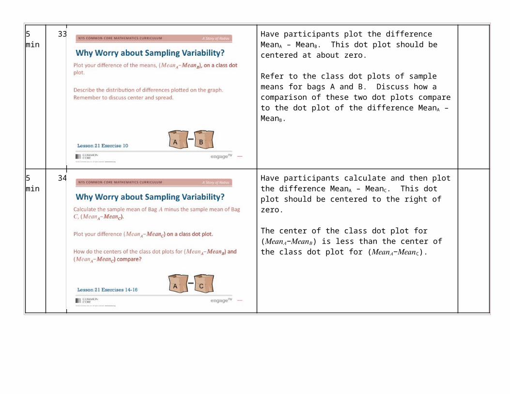
5 min 32. Help students plot their sample means on the appropriate dot plots.

Discuss the differences.

5 min 33. Have participants plot the difference MeanA – MeanB. This dot plot should be centered at about zero.

Refer to the class dot plots of sample means for bags A and B. Discuss how a comparison of these two dot plots compare to the dot plot of the difference MeanA – MeanB.

5 min 34. Have participants calculate and then plot the difference MeanA – MeanC. This dot plot should be centered to the right of zero.

The center of the class dot plot for (𝑀𝑒𝑎𝑛𝐴−𝑀𝑒𝑎𝑛𝐵) is less than the center of the class dot plot for (𝑀𝑒𝑎𝑛𝐴−𝑀𝑒𝑎𝑛C).

5 min 35. Allow participants time to discuss the question with their partner.

2 min 36. Turn to page 284 in Teacher Material.

Introduce Exercise 2.

2 min 37. Part A covers concepts in Standard 7.SP.B.3 (measuring the difference between centers).

2 min 38. Part A covers concepts in Standard 7.SP.B.4 (draw informal comparative inferences about two populations).

4 min 39. Review key points:

• Probabilities can be estimated using simulation.• The results of random samples are representative

of a population.• It is important to consider sampling variability

when comparing two populations.

Use the following icons in the script to indicate different learning modes.

Video Reflect on a prompt Active learning Turn and talk

Turnkey Materials Provided

Grade 7 Module 5 PPT Grade 7 Module 5 Faciliator Guide

Additional Suggested Resources A Story of Ratios Curriculum Overview