DSP INTEGRATED CIRCUITS STUDY NOTES

UNIT I

DIGITAL SIGNAL PROCESSING

The sampling theorem:

Due to the increased use of computers in all engineering applications, including signal

processing, it is important to spend some more time examining issues of sampling. In this

chapter we will look at sampling both in the time domain and the frequency domain

We have already encountered the sampling theorem and, arguing purely from a

trigonometric-identity point of view have established the Nyquist sampling cri-terion for

sinusoidal signals. However, we have not fully addressed the sampling of more general signals,

nor provided a general proof. Nor have we indicated how to reconstruct a signal from its

samples. With the tools of Fourier transforms and Fourier series available to us we are now

ready to nish the job that was started months ago.

To begin with, suppose we have a signal x(t) which we wish to sample. Let us suppose

further that the signal is band limited to B Hz. This means that its Fourier transform is nonzero

for- 2π B < ω < 2πB. Plot spectrum.

We will model the sampling process as multiplication of x(t) by the “picket fence" function

We encountered this periodic function when we studied Fourier series. Recall that by its Fourier

series representation we can write

Plot the spectrum of the sampled signal with both ω frequency and f frequency. Observe

the following

The spectrum is periodic, with period 2 , because of the multiple copies of the spectrum.

The spectrum is scaled down by a factor of 1=T .

Note that in this case there is no overlap between the images of the spectrum.

Now consider the effect of reducing the sampling rate to fs < 2B. In this case, the duplicates

of the spectrum overlap each other. The overlap of the spectrum is aliasing.

This demonstration more-or-less proves the sampling theorem for general signals. Provided

that we sample fast enough, the signal spectrum is not distorted by the sampling process. If we

don't sample fast enough, there will be distortion. The next question is: given a set of samples,

how do we get the signal back? From the spectrum, the answer is to filter the signal with a low-

pass filter with cutoff ωc ≥ 2πB. This cuts out the images and leaves us with the original

spectrum. This is a sort of idealized point of view, because it assumes that we are ltering a

continuous-time function x(t), which is a sequence of weighted delta functions. In practice, we

have numbers x[n] representing the value of the function x[n] = x(nT ) = x(n/fs ). How can we

recover the time function from this?

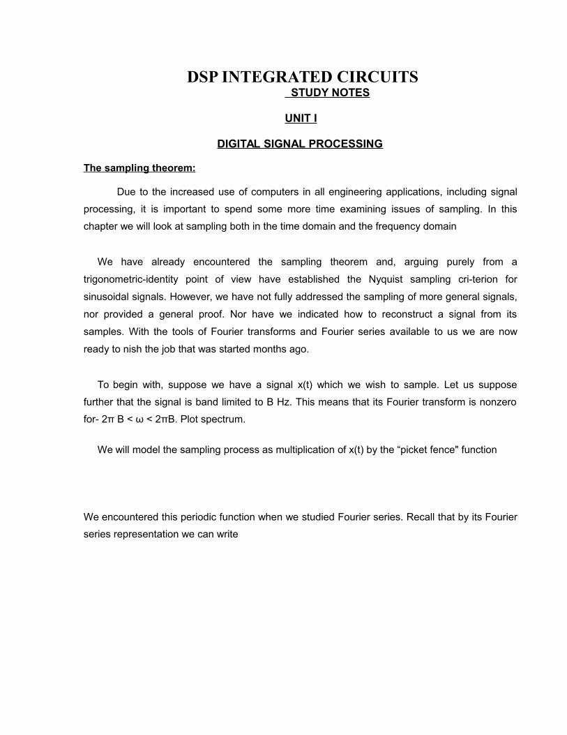
Theorem 1 (The sampling theorem)

If x(t) is band limited to B Hz then it can be recovered from signals taken at a sampling rate fs >

2B. The recovery formula is

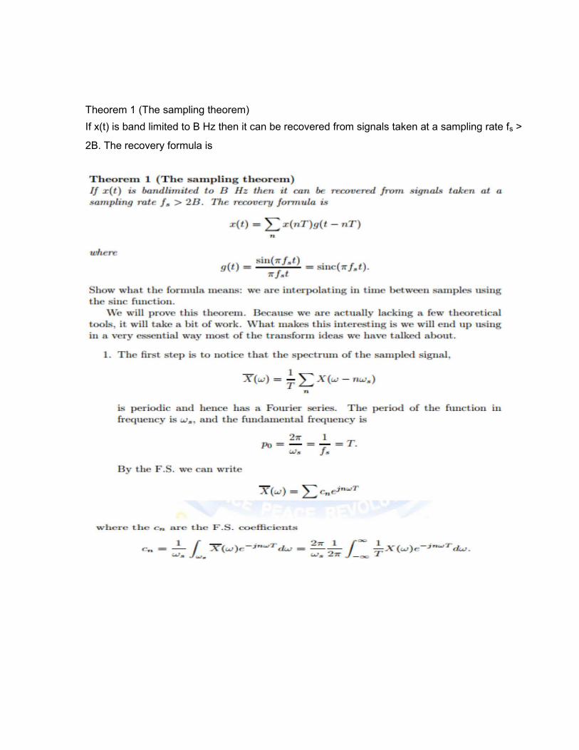
Notice that the reconstruction filter is based upon a sinc function, whose trans-form is a rect

function: we are really just doing the filtering implied by our initial intuition.

In practice, of course, we want to sample at a frequency higher than just twice the bandwidth

to allow room for filter roll off.

Adaptive DSP algorithms:

DFT-The Discrete Fourier Transform:

Introduction

The sampled discrete-time fourier transform (DTFT) of a finite length, discrete-time

signal is known as the discrete Fourier transform (DFT). The DFT contains a finite number of

samples equal to the number of samples N in the given signal. Computationally efficient

algorithms for implementing the DFT go by the generic name of fast Fourier transforms (FFTs).

This chapter describes the DFT and its properties, and its relationship to DTFT

Definition of DFT and its Inverse

Lest us consider a discrete time signal x (n) having a finite duration, say in the range 0 ≤ n ≤N-1.

The DTFT of the signal is

The result is, by definition the DFT. That is,

Equation (0.2) is known as N-point DFT analysis equation. Fig 0.1 shows the Fourier transform

of a discrete – time signal and its DFT samples.

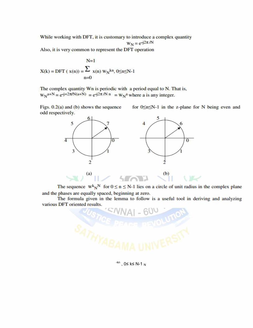
-kn , 0≤ k≤ N-1 N

Inverse DFT

The DFT values (X(k), 0≤ k≤ N-1), uniquely define the sequence x(n) through the inverse DFT

formula (IDFT) :

N-1

x (n) = IDFT (X(k) = 1 Σ X(k)

WN k=0

The above equation is known as the synthesis equation.

N-1

Proof : 1 Σ X(k) WN-kn =

N k=0N-1

=

It can be shown

that N-1

Σ WN(n-m)k =N ,

0,Hence,

N-1

1 Σ x(m) Nδ (n-m)

N

N-1 N-1

1Σ [Σ x(m) WN

km] = WN

-kn N k=0 m=0

N-1 N-1 1

Σ x(m) [Σ WN-(n-m)k]N k=0 m=0

n = mn ≠ m

= 1 x Nx (m) ( sifting property)N m=n

= x(n)

FFT-FAST FOURIER TRANSFORM:The FFT is a basic algorithm underlying much of signal processing, image processing, and

data compression. When we all start interfacing with our computers by talking to them (not

too long from now), the first phase of any speech recognition algorithm will be to digitize our

speech into a vector of numbers, and then to take an FFT of the resulting vector. So one

could argue that the FFT might become one of the most commonly executed algorithms on

most computers.

There are a number of ways to understand what the FFT is doing, and eventually we will

use all of them:

= The FFT can be described as multiplying an input vector x of n numbers by a

particular n-by-n matrix Fn, called the DFT matrix (Discrete Fourier Transform), to get

an output

vector y of n numbers: y = Fn ·x. This is the simplest way to describe the FFT, and

shows that a straightforward implementation with 2 nested loops would cost 2n2

operations. The importance of the FFT is that it performs this matrix-vector in just O(n

log n) steps using divide-and-conquer. Furthermore, it is possible to compute x from

y, i.e. compute

x = Fn−1y, using nearly the same algorithm, and just as fast. Practical uses of the FFT

require both multiplying by Fn and Fn−1.

The FFT can also be described as evaluating a polynomial with coefficients in x at a

special set of n points, to get n polynomial values in y. We will use this polynomial-

evaluation-interpretation to derive our O(n log n) algorithm. The inverse operation in

called interpolation: given the values of the polynomial y, find its coefficients x.

To pursue the signal processing interpretation mentioned above, imagine sitting down

at a piano and playing a chord, a set of notes. Each note has a characteristic

frequency (middle A is 440 cycles per second, for example). A microphone digitizing

this sound

will produce a sequence of numbers that represent this set of notes, by measuring the

air pressure on the microphone at evenly spaced sampling times t1, t2, ... , ti, where

ti = i·∆t. ∆t is the interval between consecutive samples, and 1/∆t is called the

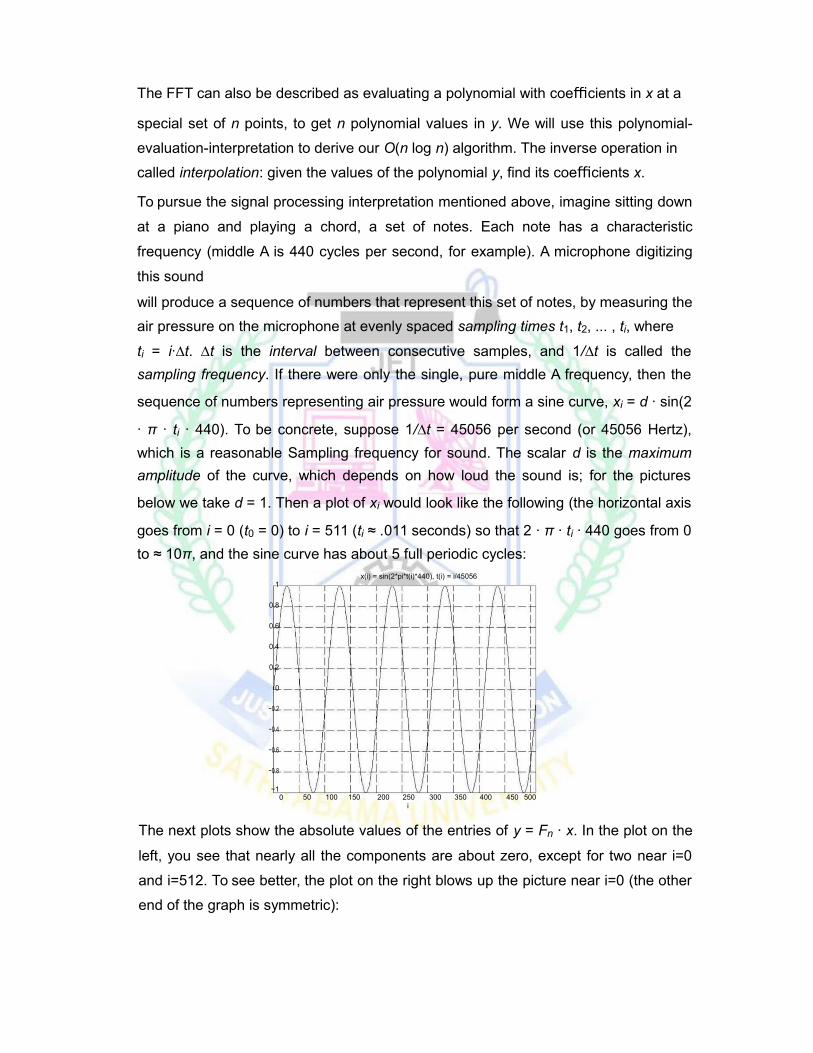
sampling frequency. If there were only the single, pure middle A frequency, then the

sequence of numbers representing air pressure would form a sine curve, xi = d · sin(2

· π · ti · 440). To be concrete, suppose 1/∆t = 45056 per second (or 45056 Hertz),

which is a reasonable Sampling frequency for sound. The scalar d is the maximum

amplitude of the curve, which depends on how loud the sound is; for the pictures

below we take d = 1. Then a plot of xi would look like the following (the horizontal axis

goes from i = 0 (t0 = 0) to i = 511 (ti ≈ .011 seconds) so that 2 · π · ti · 440 goes from 0

to ≈ 10π, and the sine curve has about 5 full periodic cycles:x(i) = sin(2*pi*t(i)*440), t(i) = i/45056

1

0.8

0.6

0.4

0.2

0

−0.2

−0.4

−0.6

−0.8

−150 100 150 200 250 300 350 400 450 5000

i

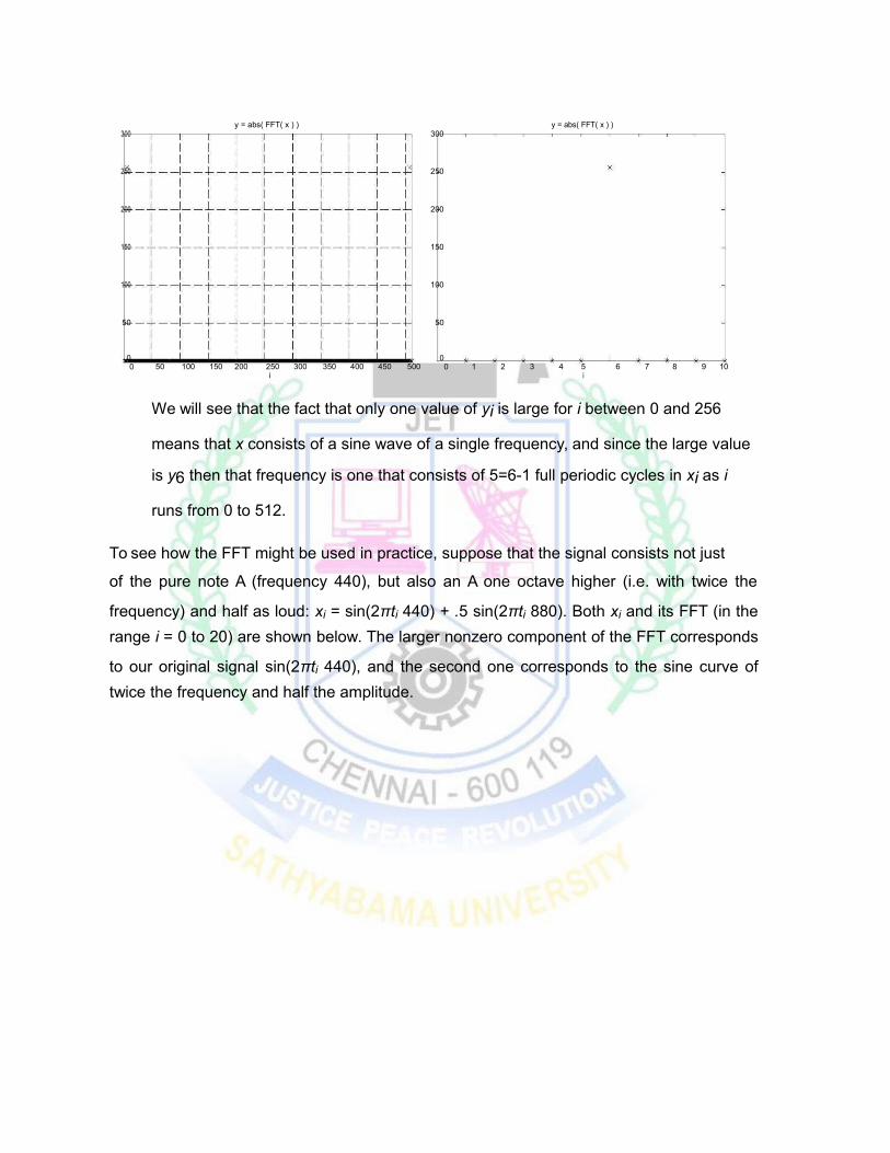
The next plots show the absolute values of the entries of y = Fn · x. In the plot on the

left, you see that nearly all the components are about zero, except for two near i=0

and i=512. To see better, the plot on the right blows up the picture near i=0 (the other

end of the graph is symmetric):

y = abs( FFT( x ) ) y = abs( FFT( x ) )300 300

250 250

200 200

150 150

100 100

50 50

050 100 150 200 250 300 350 400 450 500

01 2 3 4 5 6 7 8 9 100 0

i i

We will see that the fact that only one value of yi is large for i between 0 and 256

means that x consists of a sine wave of a single frequency, and since the large value

is y6 then that frequency is one that consists of 5=6-1 full periodic cycles in xi as i

runs from 0 to 512.

To see how the FFT might be used in practice, suppose that the signal consists not just

of the pure note A (frequency 440), but also an A one octave higher (i.e. with twice the

frequency) and half as loud: xi = sin(2πti 440) + .5 sin(2πti 880). Both xi and its FFT (in the

range i = 0 to 20) are shown below. The larger nonzero component of the FFT corresponds

to our original signal sin(2πti 440), and the second one corresponds to the sine curve of

twice the frequency and half the amplitude.

1.5

1

0.5

0

−0.5

−1

−1.50

Sum of two sine curves abs( FFT( Sum of two sine curves ) )300

250

200

150

100

50

50 100 150 200 250 300 350 400 450 50000 2 4 6 8 10 12 14 16 18 20

i i

But suppose that there is “noise” in the room where the microphone is recording the

piano, which makes the signal xi “noisy” as shown below to the left (call it x_i). (In this

example we added a random number between −.5 and .5 to each xi to get x_i.) x and

x_ appear very different, so that it would seem difficult to recover the true x from noisy

x_. But by examining the FFT of x_i below, it is clear that the signal still mostly consists

of two sine waves. By simply zeroing out small components of the FFT of x_

(those below the “noise level”) we can recover the FFT of our two pure sine curves,

and then get nearly the original signal x(i) back. This is a very simple example of

filtering, and is discussed further in other EE courses.

Noisy sum of two sine curves abs( FFT( noisy sum of two sine curves ) )1.5 300

1 250

0.5 200

0 150

−0.5 100

−1 50

−1.550 100 150 200 250 300 350 400 450 500

00 0 2 4 6 8 10 12 14 16 18 20

i i

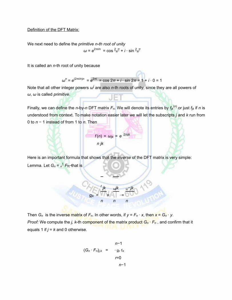
Definition of the DFT Matrix:

We next need to define the primitive n-th root of unity

ω = e2πi/n = cos 2nπ + i · sin 2n

π

It is called an n-th root of unity because

ωn = e(2πi/n)n = e2πi = cos 2π + i · sin 2π = 1 + i · 0 = 1

Note that all other integer powers ωj are also n-th roots of unity; since they are all powers of

ω, ω is called primitive.

Finally, we can define the n-by-n DFT matrix Fn. We will denote its entries by fjk(n) or just fjk if n is

understood from context. To make notation easier later we will let the subscripts j and k run from

0 to n − 1 instead of from 1 to n. Then

f (n) = ωjk = e 2πijk

n jk

Here is an important formula that shows that the inverse of the DFT matrix is very simple:

Lemma. Let Gn = n1 Fn, that is

f jk ωjk ω−jk

gjk = = =n n n

Then Gn is the inverse matrix of Fn. In other words, if y = Fn · x, then x = Gn · y.

Proof: We compute the j, k-th component of the matrix product Gn · Fn , and confirm that it

equals 1 if j = k and 0 otherwise.

n−1

(Gn · Fn)j,k = _ gjr frk

r=0

n−1

= 1 _ f¯jr frk n r=0

N-1 Similarly, x (n) Σ X (k) WN-kn

k=0

N-1⇒ x (n+N) = 1 Σ X(k) WN

-k(n+N)

N k=0

N-1

= 1 Σ X(k) WN-kn WN -kn

N k=0

Since, WN-kn = e-j2π/N kN = e-j2πk = 1, we get

N-1

x(n+N) = 1 Σ X(k) WN-kn =

x (n)

Since, DFT and its inverse are both periodic with period N, it is sufficient to compute the

results for one period (0 to N-1). We want to emphasize that both x (n) and X (k) have a starting

index of zero.

A very important implication of x (n), being periodic is, if we wish to find DFT of a periodic

signal, we extract one period of the periodic signal and then compute its DFT.

Interpreting y = Fn · x as polynomial evaluation:

By examining the formula for yj in y = Fn · x we see

n−1 n−1

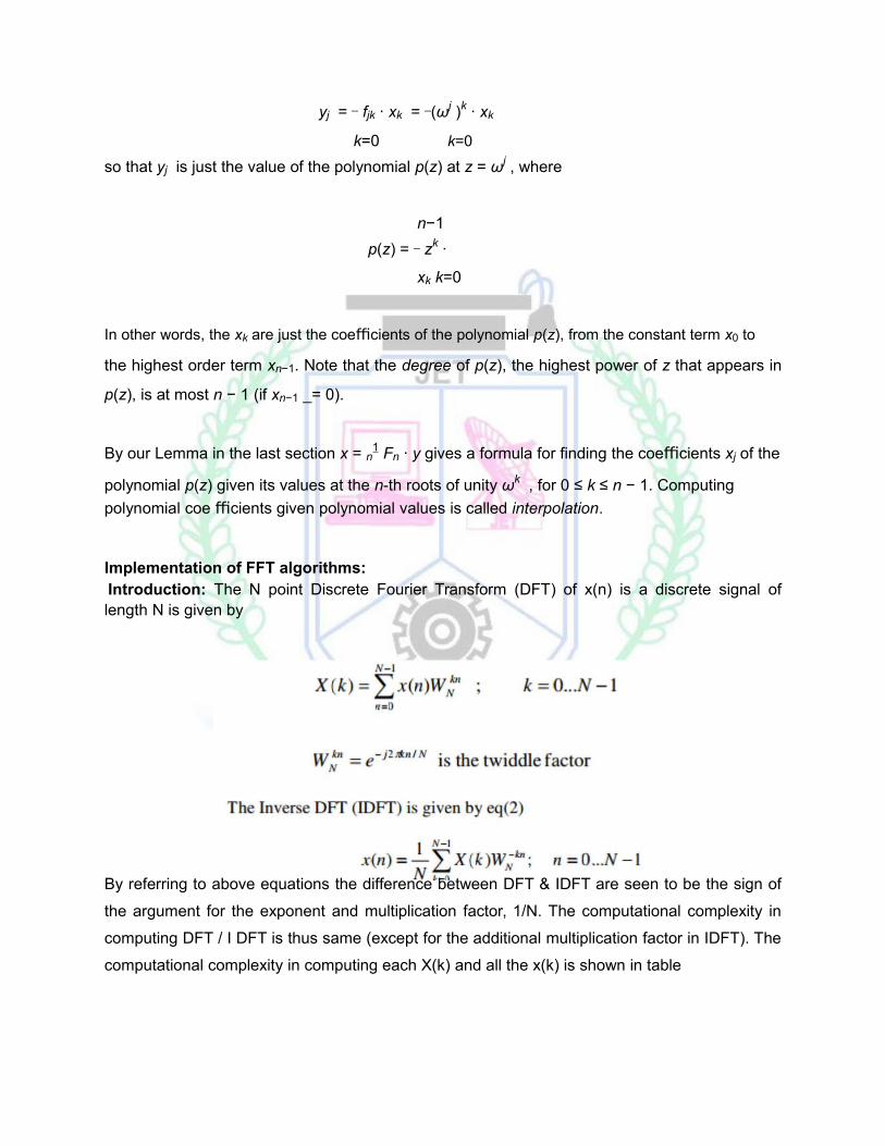
yj = _ fjk · xk = _(ωj )k · xk

k=0 k=0

so that yj is just the value of the polynomial p(z) at z = ωj , where

n−1

p(z) = _ zk ·

xk k=0

In other words, the xk are just the coefficients of the polynomial p(z), from the constant term x0 to

the highest order term xn−1. Note that the degree of p(z), the highest power of z that appears in

p(z), is at most n − 1 (if xn−1 _= 0).

By our Lemma in the last section x = n1 Fn · y gives a formula for finding the coefficients xj of the

polynomial p(z) given its values at the n-th roots of unity ωk , for 0 ≤ k ≤ n − 1. Computing

polynomial coe fficients given polynomial values is called interpolation.

Implementation of FFT algorithms:Introduction: The N point Discrete Fourier Transform (DFT) of x(n) is a discrete signal oflength N is given by

By referring to above equations the difference between DFT & IDFT are seen to be the sign of

the argument for the exponent and multiplication factor, 1/N. The computational complexity in

computing DFT / I DFT is thus same (except for the additional multiplication factor in IDFT). The

computational complexity in computing each X(k) and all the x(k) is shown in table

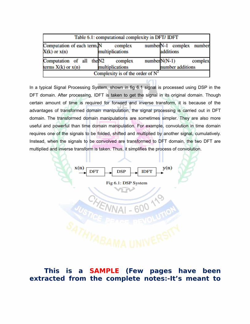
In a typical Signal Processing System, shown in fig 6.1 signal is processed using DSP in the

DFT domain. After processing, IDFT is taken to get the signal in its original domain. Though

certain amount of time is required for forward and inverse transform, it is because of the

advantages of transformed domain manipulation, the signal processing is carried out in DFT

domain. The transformed domain manipulations are sometimes simpler. They are also more

useful and powerful than time domain manipulation. For example, convolution in time domain

requires one of the signals to be folded, shifted and multiplied by another signal, cumulatively.

Instead, when the signals to be convolved are transformed to DFT domain, the two DFT are

multiplied and inverse transform is taken. Thus, it simplifies the process of convolution.

This is a SAMPLE (Few pages have beenextracted from the complete notes:-It’s meant to

show you the topics covered in the full notes andas per the course outline

Download more at our websites:www.naarocom.com

To get the complete notes either in softcopy form or in Hardcopy (printed & Binded) form, contact us on:

Call/text/whatsApp +254 719754141/734000520

Email:

naarocom@gmail.cominfo@naarocom.comsales@naarocom.com

Get news and updates by liking ourpage on facebook and follow us on

Twitter

Sample/preview is NOT FOR SALE