Downscaling of global solar irradiation in complexareas in R

F. Antonanzas-Torres∗Edmans Group

ETSII, University of La Rioja, Logroño, Spain

F. J. Martínez-de-PisónEdmans Group

ETSII, University of La Rioja, Logroño, Spain

J. AntonanzasEdmans Group

ETSII, University of La Rioja, Logroño, Spain

O. PerpinanElectrical Engineering Department

ETSIDI, Universidad Politecnica de Madrid, Spain

September 15, 2014

Abstract

A methodology for downscaling solar irradiation from satellite-derived databasesis described using R software. Different packages such as raster, parallel, solaR,gstat, sp and rasterVis are considered in this study for improving solar resourceestimation in areas with complex topography, in which downscaling is a very use-ful tool for reducing inherent deviations in satellite-derived irradiation databases,which lack of high global spatial resolution. A topographical analysis of horizonblocking and sky-view is developed with a digital elevation model to determinewhat fraction of hourly solar irradiation reaches the Earth’s surface. Eventually,kriging with external drift is applied for a better estimation of solar irradiationthroughout the region analyzed including the use of local measurements. Thismethodology has been implemented as an example within the region of La Rioja innorthern Spain. The mean absolute error found using the methodology proposedis 91.92 kWh/m2, vs. 172.62 kWh/m2 using the original satellite-derived database(a striking 46.75% lower). The code is freely available without restrictions for fu-ture replications or variations of the study at https://github.com/EDMANSolar/downscaling.

Keywords: Solar irradiation, R, raster, solaR, digital elevation model, shadeanalysis, downscaling.

∗Corresponding author: antonanzas.fernando@gmail.com

1

1 Introduction

During the last few years the development of photovoltaic energy has flourished indeveloping countries with both multi-megawatt power plants and micro installations.However, the scarcity of long-term, reliable solar irradiation data from pyranometersin many of these countries makes it necessary to estimate solar irradiation from othermeteorological variables or satellite images [Schulz et al., 2009; Polo et al., 2014; Vindelet al., 2013]. In such cases, meteorological or satellite derived models need to be vali-dated via nearby pyranometer records, since they lack spatial generalization. Thus, insome regions in which there are no pyranometers nearby these models are ruled outas an option and irradiation data must be obtained from satellite estimates. Althoughsatellite-derived irradiation databases such as NASA’s Surface meteorology and SolarEnergy (SSE)1, the National Renewable Energy Laboratory (NREL)2, INPE3, SODA4

and the Climate Monitoring Satellite Application Facility (CM SAF)5 provide wide spa-tial coverage, only NASA and some CM SAF climate data sets give global coverage,albeit at a reduced spatial resolution (Table 1).

Satellite estimates tend to average solar irradiation and omit the impact of topog-raphy within each cell, which generally are in the range of kilometers. As a result,intra-cell variations can be significant in areas with local micro-climatic characteristicsand in areas with complex topography (which are often one and the same) [Bosch et al.,2010]. In this case, the irradiation data might not be accurate enough to enable a pho-tovoltaic installation to be designed. [Perez et al., 1994] analyze the spatial behavior ofsolar irradiation and conclude that the threshold distance from satellite estimates is inthe order of 7 km. [Antonanzas-Torres et al., 2013a] reject ordinary kriging as a spatialinterpolation method for solar irradiation in Spain with stations more than 50 km apartin mountainous regions, as a result of the high spatial variability of solar radiation insuch areas. The NASA-SSE and CM SAF SIS Climate Data Sets provide global hori-zontal irradiation (GHI) with global coverage with resolutions of 1x1◦ and 0.25x0.25◦

(Table 1), which in most latitudes implies a grosser resolution than the previously men-tioned 40-50 km.

The influence of terrain has not been widely implemented in satellite-derived solarirradiation databases although it is well known that complex topography attenuatessolar irradiation due to shadowing, sky-view (portion of visible sky) and ground re-flectance [Ruiz-Arias et al., 2010]. The incoming solar irradiation not blocked by terrainalso varies at different solar elevations due to the atmospheric attenuation by aerosolsand water vapor (being the influence higher at lower elevations). As a result, complextopography affects micro-climate and makes solar irradiation estimation more complexthan in flat areas. For this reason, the analysis of solar irradiation with high spatial res-olution is very interesting in areas with complex terrain.

1http://maps.nrel.gov/SWERA2http://www.nrel.gov/gis/solar.html3http://www.inpe.br4http://www.soda-is.com/eng/index.html5http://www.cmsaf.eu

2

One of the alternatives for obtaining higher spatial resolution of solar irradiation isthe downscaling of satellite estimates. Irradiation downscaling can be based on interpo-lation kriging techniques when pyranometer records are available, with the implemen-tation of continuous irradiation-related variables such as elevation, sky-view-factor [Al-samamra et al., 2009; Batlles et al., 2008] and other meteorological variables (i.e. temper-ature gradient and rainfall) as external drifts [Antonanzas-Torres et al., 2013b]. Down-scaling is generally based on digital elevation models (DEM) with satellite-derived ir-radiation data to account for the effect of complex topography. It has previously beenapplied in mountainous areas such as the Mont Blanc Massif (France) [Corripio, 2003]and Sierra Nevada (Spain) [Bosch et al., 2010; Ruiz-Arias et al., 2010] with image res-olutions of 3.5x3.5 km. Influence of topography for shade analysis has also been im-plemented in geographical information systems for solar irradiation modeling, such asr.sun [Suri and Hofierka, 2004] with simplified atmospheric parametrizations, whichlimit accuracy [Ruiz-Arias et al., 2009].

However, the NASA-SSE and CM SAF SIS Climate Data Sets are based on muchlower resolutions and are the only irradiation datasets in numerous countries wherethere has been recent interest in solar energy. In this paper, a downscaling methodologyof global solar irradiation is explained by means of R software and studied in the regionof La Rioja (a mountainous region in northern Spain).

In a first step, hourly data from the CM SAF with 0.03x0.03◦ resolution is down-scaled to a higher resolution (200x200 m). In a second step, kriging with external drift,also referred to as universal kriging, is applied to interpolate data from 6 on-groundpyranometers in the region, and this downscaled CM SAF data is considered as an ex-planatory variable. The evaluation of the proposed method is performed with on-sitemeasured GHI. Finally, a downscaled map of annual global solar radiation throughoutthis region is obtained.

2 Data

The CM SAF was funded in 1992 as a joint venture of several European meteorologicalinstitutes, with the collaboration of the European Organization for the Exploitation ofMeteorological Satellites (EUMETSAT) to retrieve, archive and distribute climate datato be used for climate monitoring and climate analysis [Trentmann et al., 2011; Schulzet al., 2009]. CM-SAF provides satellite-based operational products and climate data(using the nomenclature by the CM SAF). Operational products are built on data vali-dated with on-ground stations and provided in near-to-present time and climate dataare long-term series for evaluating inter-annual variability. This study is built on hourlysurface incoming solar radiation and direct irradiation climate data, denoted as SIS andSID by CM SAF respectively, for the year 2005. These climate data are derived fromMeteosat first generation satellites (Meteosat 2 to 7, 1982-2005) and validated usingon-ground records from the Baseline Surface Radiation Network (BSRN) as a reference.The validation threshold monthly mean absolute bias of SIS and SID is 15 and 20 W/m2

[Posselt et al., 2012], providing a maximum spatial resolution of 0.03x0.03◦. The high

3

reflectivity of bright surfaces (i.e. snow covered areas, deserts, and salty areas) leadsto a higher uncertainty in the calculation of SIS. The CM SAF uses an algorithm basedon fuzzy logic, which specifically improves the estimation in these bright areas [Trent-mann et al., 2011]. In the study, SIS and SID data are selected with spatial resolutionof 0.03x0.03◦. Data is freely accessible via FTP through the CM SAF website. HourlyGHI records from SOS Rioja6, taken from 6 meteorological stations (shown in Figure 1and Table 2) in 2005 serve as complementary measurements for downscaling within theregion studied. These stations have First Class pyranometers (according to ISO 9060)with uncertainty levels of 5% in daily totals. These data are filtered from spurious (notavailable data and values with atmospheric transmittivity- relation between GHI andextra-terrestrial solar irradiation higher than 0.85), assuming when relevant the aver-age between the previous and following hourly measurements. The digital elevationmodel (DEM) is also freely obtained from product MDT-200 by the c©Spanish Instituteof Geography7 with a spatial resolution of 200x200 m.

Four meteorological stations, 1, 2, 4 and 6, (corresponding to Ezcaray, Logroño,San Roman and Yerga) are used in the downscaling and data from stations 3 and 5(Moncalvillo and Ventrosa) are used for testing the downscaling proposed.

3 Method

This section has been divided into three subsections based on the irradiation decom-position, sky view factor and horizon blocking and finally, the post-processing withkriging with external drift.

3.1 Irradiation decomposition

Initially, diffuse horizontal irradiation (DHI) is obtained from the difference betweenglobal horizontal irradiation (GHI) and beam horizontal irradiation (BHI) rasters, pre-viously obtained from CM SAF. DHI and BHI are firstly disaggregated from the origi-nal gross resolution (0.03x0.03◦) into the DEM resolution (200x200 m) using the bilinearmethod. In a second step, DHI is divided in two components: isotropic diffuse irra-diation (DHIiso), and anisotropic diffuse irradiation (DHIani) as per the model by Hay& Mckay [Hay and Mckay, 1985] (Equation 1). This model is based on the anisotropyindex (k1), defined as the ratio of the beam irradiance (B(0)) to the extra-terrestrialirradiance (B0(0)), as shown in Equation 2. High k1 values are typical in clear sky at-mospheres, while low k1 values are frequent in overcast atmospheres and those with ahigh aerosol density.

DHI = DHIiso + DHIani (1)

6http://www.larioja.org/npRioja/default/defaultpage.jsp?idtab=4428217http://www.ign.es

4

k1 =B(0)B0(0)

(2)

The DHIiso accounts for the incoming diffuse irradiation portion from an isotropicsky, being higher with higher cloudiness (Equation 3).

DHIiso = DHI · (1− k1) (3)

DHIani, also denoted as circumsolar diffuse irradiation, considers the incoming por-tion from the circumsolar disk, which is area surrounding the solar disk. It can be ana-lyzed as beam irradiation [Perpiñán-Lamigueiro, 2013] (Equation 4).

DHIani = DHI · k1 (4)

3.2 Sky view factor and horizon blocking

Topographical analysis is performed accounting for the visible sky sphere (sky view)and horizon blocking. The DHIiso is directly dependent on the sky-view factor (SVF),which computes the proportion of visible sky related to a flat horizon. The sky-viewfactor is considered in earlier irradiation assessments [Ruiz-Arias et al., 2010; Corri-pio, 2003]. It is calculated in each DEM pixel by considering 72 vectors (separated by5◦ each) and evaluating the maximum horizon angle (θhor) over 20 km in each vector(Equation 5). The θhor stands for the maximum angle between the altitude of a locationand the elevation of the group of points along each vector, related to a horizontal planeon the location. Locations without horizon blocking have SVFs close to 1, which meansa whole visible semi-sphere of sky.

SVF = 1−∫ 2π

0sin2θhordθ (5)

Eventually, the downscaled DHIiso (DHIiso,down) is computed with Equation 6.

DHIiso,down = DHIiso · SVF (6)

Horizon blocking is analyzed by evaluating the solar geometry in 15 minute sam-ples, particularly the solar elevation (γs) and the solar azimuth (ψs). Secondly, the meanhourly γs and ψs (from those 15 minute rasters) are calculated and then disaggregatedas explained above for DHI and BHI rasters. The θhor corresponding to each ψs is com-pared with the γs. As a consequence, if the γs is lower than the θhor, then there is horizonblocking on the surface analyzed and therefore, BHI and DHIani are blocked. Finally,the sum of DHIani,down, DHIiso,down and BHIiso,down constitutes the downscaled globalhorizontal irradiation GHIdown.

5

3.3 Post-processing: kriging with external drift

The fact that this downscaling accounts for the irradiation loss due to horizon block-ing and the sky-view factor leads us to introduce a trend in estimates (lowering them)compared to the original data (gross resolution data). However, satellite-derived irra-diation data implicitly considers shade, as a consequence of the lower albedo recordedin these zones, but it is later averaged over the pixel. GHIdown is used as the raster layerwith the shading behavior on solar irradiation within the region studied. Universal krig-ing or kriging with external drift (KED) includes information from exhaustively-sampledexplanatory variables in the interpolation. As a result, GHIdown is considered as theexplanatory variable for interpolating measured irradiation data from on-ground cal-ibrated pyranometers, which is denoted as post-processing. GHIdown is correlated withthe DEM as a consequence of the major influence of horizon blocking with topography,estimations can be derived by separating the deterministic and stochastic components(Equation 7).

z(sθ) =p

∑k=0

βkqk(sθ)︸ ︷︷ ︸deterministic

+n

∑i=1

λiε(si)︸ ︷︷ ︸stochastic

(7)

where z(sθ) is the estimated value in sθ , βk are the estimated coefficients of thedeterministic model, qk(sθ) are the auxiliary predictors obtained from the fitted valuesof the explanatory variable at the new location, λi are the kriging weights determinedby the spatial dependence structure of the residual, and ε(si) are the residual at locationsi [Antonanzas-Torres et al., 2013a].

The semivariogram is a function defined as Equation 8 based on a constant varianceof ε and also on the assumption that spatial correlation of ε depends on the distanceamongst instances (h) rather than on their position [Pebesma, 2004].

γ(h) =12

E[ε(s)− ε(s + h)]2 (8)

Given that the above sample variogram only collates estimates from observed points,a fitting model of this variogram is generally considered to extrapolate the spatial be-havior of observed points to the area studied. Different variogram functions are com-monly defined such as the exponential, Gaussian or spherical models. Along theseequations, different parameters such as the sill, range and nugget of the model mustbe adjusted to best fit the sample variogram [Hengl, 2009]. The nugget effect, generallyassociated with intrinsic micro-variability and measurement error, models the disconti-nuity of the variogram at the source. It must be highlighted that when the nugget effectis recorded, estimates are different from measured values in the stations. The variogrammodel of solar horizontal irradiation is evaluated in Spain, and the conclusion reachedis that a pure nugget fitting behaves best, which implies no spatial auto-correlation onresiduals [Antonanzas-Torres et al., 2013a].

6

Figure 2 displays the method diagram using red ellipses and lines for data sources,blue ellipses and lines for derived rasters (results), and black rectangles and lines foroperations.

The mean absolute error (MAE), root mean square error (RMSE) and mean bias error(MBE), described in Equations 9, 10 and 11, are used as indicators of models deviation.

MAE =∑n

i=1 |xest − xmeas|n

(9)

RMSE =

√∑n

i=1 (xest − xmeas)2

n(10)

MBE =∑n

i=1 xest − xmeas

n(11)

where n is number of stations and xest and xmeas the annual estimated and measuredirradiation, respectively.

4 Implementation

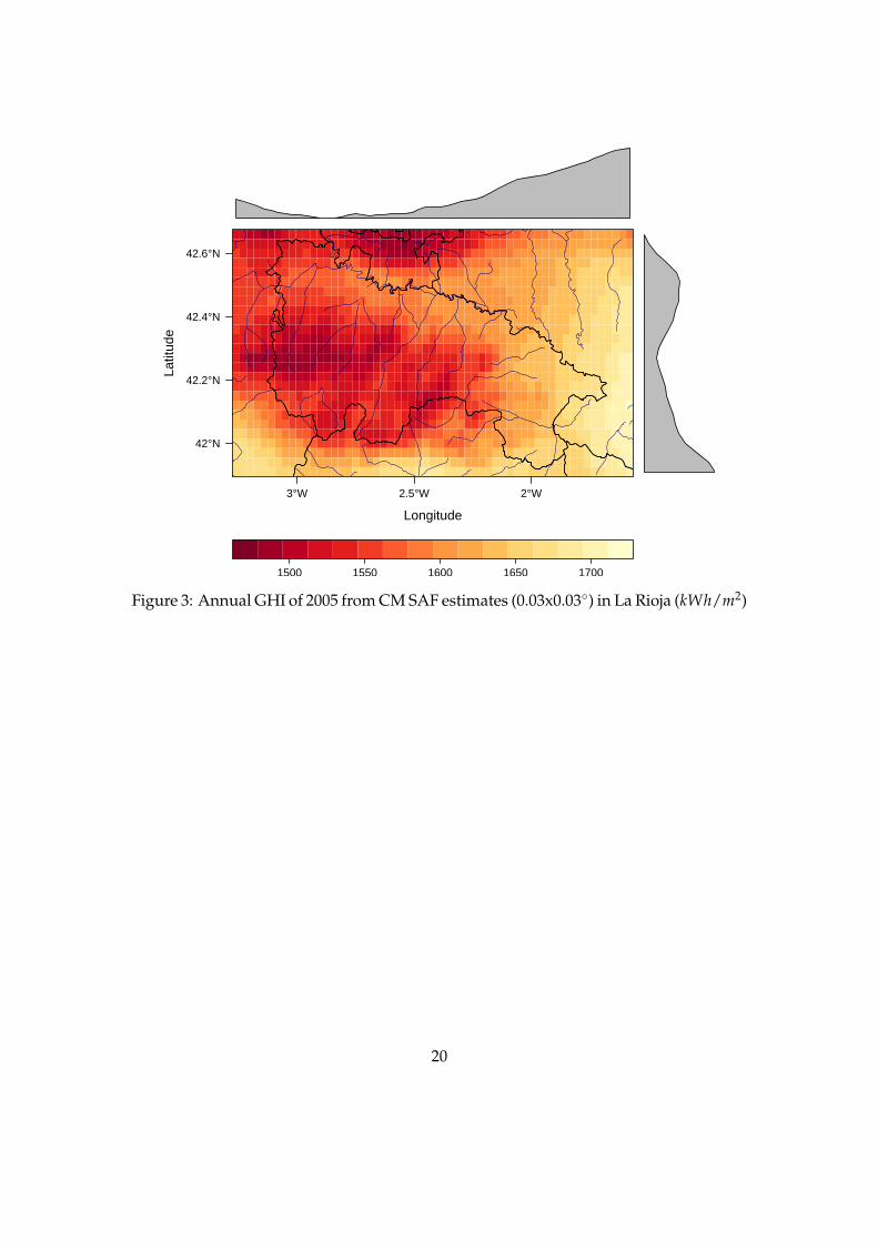
The method proposed is applied in the region of La Rioja (northern Spain). Figure3 shows the corresponding annual global horizontal irradiation from CM SAF withresolution 0.03x0.03◦.

4.1 Packages

The downscaling described in this paper has been implemented using the free softwareenvironment R [R Development Core Team, 2013] and various contributed packages:

• raster [Hijmans and van Etten, 2013] for spatial data manipulation and analysis.

• solaR [Perpiñán-Lamigueiro, 2012] for solar geometry.

• gstat [Pebesma and Graeler, 2013] and sp [Pebesma et al., 2013] for geostatisticalanalysis.

• parallel for multi-core parallelization.

• rasterVis [Perpiñán-Lamigueiro and Hijmans, 2013] for spatial data visualiza-tion methods.

R> library(sp)R> library(raster)R> rasterOptions(todisk=FALSE)R> rasterOptions(chunksize = 1e+06, maxmemory = 1e+07)R> library(maptools)R> library(gstat)

7

R> library(lattice)R> library(latticeExtra)R> library(rasterVis)R> library(solaR)R> library(parallel)

4.2 Data

Satellite data can be freely downloaded after registration from CM SAF8 by going tothe data access area, selecting web user interface and climate data sets and then choosingthe hourly climate data sets named SIS (Global Horizontal Irradiation)) and SID (BeamHorizontal Irradiation) for 2005. Both rasters are projected to the UTM projection forcompatibility with the DEM.

R> projUTM <- CRS(’+proj=utm␣+zone=30’)R> projLonLat <- CRS(’␣+proj=longlat␣+ellps=WGS84’)

R> listFich <- dir(pattern=’SIShm2005’)R> stackSIS <- stack(listFich)R> stackSIS <- projectRaster(stackSIS,crs=projUTM)

R> listFich <- dir(pattern=’SIDhm2005’)R> stackSID <- stack(listFich)R> stackSID <- projectRaster(stackSID, crs=projUTM)

We compute the annual global irradiation, which will be used as a reference forsubsequent steps.

R> SISa2005 <- calc(stackSIS, sum, na.rm=TRUE)

The Spanish Digital Elevation Model can be obtained after registration from thec©Spanish Institute of Geography9 by going to the free download of digital geographic

information for non-commercial use area, and then cropping to the region analyzed (LaRioja). As stated above, this DEM uses the UTM projection.

R> elevSpain <- raster(’elevSpain.grd’)R> elev <- crop(elevSpain, extent(479600, 616200, 4639600, 4728400))R> names(elev)<-’elev’

4.3 Sun geometry

The first step is to compute the sun angles (height and azimuth) and the extraterres-trial solar irradiation for each cell of the CM SAF rasters. The function calcSol fromthe solaR package calculates the daily and intradaily sun geometry. By means of thisfunction and overlay from the raster package, three multilayer raster objects are

8www.cmsaf.eu9http://www.ign.es

8

generated with the sun geometry needed for the next steps. For the sake of brevity weshow only the procedure for extraterrestrial solar irradiation. The sun geometry is cal-culated with the spatial resolution of CM SAF (0.03x0.03o). First, it is defined a functionto extract the hour for aggregation, choose the annual irradiation raster as reference,and define a raster with longitude and latitude coordinates.

R> hour <- function(tt)as.POSIXct(trunc(tt, ’hours’))

R> r <- SISa2005

R> latlon <- stack(init(r, v=’y’), init(r, v=’x’))R> names(latlon) <- c(’lat’, ’lon’)

The extraterrestrial irradiation is calculated with 5-min samples. Each point is acolumn of the data frame locs. Its columns are traversed with lapply, so for eachpoint of the raster object a time series of extraterrestrial solar irradiation is computed.The result, B05min, is a RasterBrick object with a layer for each element of the timeindex BTi, which is aggregated to an hourly raster with zApply and transformed to theUTM projection.

R> BTi <- seq(as.POSIXct(’2005-01-01␣00:00:00’),+ as.POSIXct(’2005-12-31␣23:55:00’), by=’5␣min’)

R> B05min <- overlay(latlon, fun=function(lat, lon){+ locs <- as.data.frame(rbind(lat, lon))+ b <- lapply(locs, function(p){++ hh <- local2Solar(BTi, p[2])+ sol <- calcSol(p[1], BTi=hh)+ Bo0 <- as.data.frameI(sol)$Bo0+ Bo0 })+ res <- do.call(rbind, b)})

R> B05min <- setZ(B05min, BTi)R> names(B05min) <- as.character(BTi)

R> B0h <- zApply(B05min, by=hour, fun=mean)R> projectRaster(B0h,crs=projUTM)

4.4 Irradiation components

The CM SAF rasters must be transformed to the higher resolution of the DEM (UTM200x200 m). Because of the differences in pixel geometry between DEM (square) andirradiation rasters (rectangle) the process is performed in two steps.

The first step increases the spatial resolution of the irradiation rasters to a largerpixel size than the DEM with disaggregated data, where sf is the scale factor. Thesecond step post-processes the previous step by means of a bilinear interpolation which

9

resamples the raster layer and achieves the same DEM resolution (resample). This two-step disaggregation prevents the loss of the original values of the gross resolution rasterthat would be directly interpolated with the one-step disaggregation.

R> sf <- res(stackSID)/res(elev)

R> SIDd <- disaggregate(stackSID, sf)R> SIDdr <- resample(SIDd, elev)

R> SISd <- disaggregate(stackSIS, sf)R> SISdr <- resample(SISd, elev)

The diffuse irradiation is obtained from the global and beam irradiation rasters. Thetwo components of the diffuse irradiation, isotropic and anisotropic, can be separatedwith the anisotropy index, computed as the ratio between beam and extraterrestrialirradiation.

R> Difdr <- SISdr - SIDdr

R> B0hd <- disaggregate(B0h, sf)R> B0hdr <- resample(B0hd, elev)

R> k1 <- SIDdr/B0hdr

R> Difiso <- (1-k1) * DifdrR> Difani <- k1 * Difdr

4.5 Sky view factor and horizon blocking

4.5.1 Horizon angle

The maximum horizon angle required for the horizon blocking analysis and to derivethe SVF is obtained with the next code. The alpha vector is visited with mclapply (usingparallel computing). For each direction angle (elements of this vector) the maximumhorizon angle is calculated for a set of points across that direction from each of the lo-cations defined in xyelev (derived from the DEM raster and transformed in the matrixlocs visited by rows).

R> xyelev <- stack(init(elev, v=’x’),+ init(elev, v=’y’),+ elev)R> names(xyelev) <- c(’x’, ’y’,’elev’)

R> inc <- pi/36R> alfa <- seq(-0.5*pi,(1.5*pi-inc), inc)

R> locs <- as.matrix(xyelev)

10

Separations between the source locations and points along each direction are de-fined by resD, the maximum resolution of the DEM, d, maximum distance to visit, andconsequently in the vector seps.

R> resD <- max(res(elev))

R> d <- 20000R> seps <- seq(resD, d, by=resD)

The elevation (z1) of each point in xyelev is converted into the horizon angle: thelargest of these angles is the horizon angle for that direction. The result of each applystep is a matrix, which is used to fill in a RasterLayer (r). The result of mclapply is alist, hor, of RasterLayer which can be converted into a RasterStack with stack. Eachlayer of this RasterStack corresponds to a different direction.

R> hor <- mclapply(alfa, function(ang){+ h <- apply(locs, 1, function(p){+ x1 <- p[1]+cos(ang)*seps+ y1 <- p[2]+sin(ang)*seps+ p1 <- cbind(x1,y1)+ z1 <- elevSpain[cellFromXY(elevSpain,p1)]+ hor <- r2d(atan2(z1-p[3], seps))+ maxHor <- max(hor[which.max(hor)], 0)+ })+ r <- raster(elev)+ r[] <- matrix(h, nrow=nrow(r), byrow=TRUE)+ r}, mc.cores=8)R> horizon <- stack(hor)

This operation is very time-consuming as it is necessary to work with high resolu-tion files. Computation time can be decreased by increasing the sampling space (200m) or the sectoral angle (5 ◦) or by reducing the maximum distance (20 km).

4.5.2 Horizon blocking

Horizon blocking is analyzed by evaluating the solar geometry in 15 minute samples,particularly the solar elevation and azimuth angles from the original irradiation raster.Secondly, the hourly averages are calculated, disaggregated and post-processed as ex-plained above for the irradiation rasters. The decision to solve the solar geometry withlow resolution rasters enables a significant reduction to be obtained in computationtime without penalizing the results.

First, the azimuth raster is cut into different classes according to the alpha vector(directions). The values of the horizon raster corresponding to each angle class areextracted using stackSelect.

R> idxAngle <- cut(AzShr, breaks=r2d(alfa))R> AngAlt <- stackSelect(horizon, idxAngle)

11

The number of layers of AngAlt is the same as idxAngle and can therefore be usedfor comparison with the solar height angle, AlShr. If AngAlt is greater, there is horizonblocking (dilogical=0).

R> dilogical <- ((AngAlt-AlShr) < 0)

With this binary raster, beam irradiation and diffuse anisotropic irradiation can becorrected with horizon blocking.

R> Dirh <- SIDdr * dilogicalR> Difani <- Difani * dilogical

4.5.3 Sky view factor

The sky-view factor can be easily computed from the horizon object with the equation5. This factor corrects the isotropic component of the diffuse irradiation.

R> SVFRuizArias <- calc(horizon, function(x) sin(d2r(x))^2)R> SVF <- 1 - mean(SVFRuizArias)

R> Difiso <- Difiso * SVF

Finally, the global irradiation is the sum of the three corrected components, beamand anisotropic diffuse irradiation including horizon blocking, and isotropic diffuseirradiation with the sky view factor.

R> GHIh <- Difanis + Difiso + DirhR> GHI2005a <- calc(GHIh, fun=sum)

4.6 Kriging with external drift

The downscaled irradiation rasters can be improved by using kriging with externaldrift. Irradiation data from on-ground meteorological stations is interpolated with thedownscaled irradiation raster as the explanatory variable. To define the variogram herewe use the results previously published in [Antonanzas-Torres et al., 2013a].

R> load(’Stations.RData’)R> UTM <- SpatialPointsDataFrame(Stations[,c(2,3)], Stations[,-c(2,3)],+ proj4string=CRS(’+proj=utm␣+zone=30␣+ellps=WGS84’))

The file Stations.RData contains information regarding annual measured and CMSAF GHI (GHImed and GHICMSAF, respectively). For a better insight of this file it is pro-vided at https://github.com/EDMANSolar/downscaling. The variogram is built usingthe spatial data of the SpatialPointsDataFrame object and the nugget model.

R> vgmCMSAF <- variogram(GHImed ~ GHIcmsaf, UTM)R> fitvgmCMSAF <- fit.variogram(vgmCMSAF, vgm(model=’Nug’))

12

R> gModel <- gstat(NULL, id=’G0yKrig’,+ formula= GHImed ~ GHIcmsaf,+ locations=UTM, model=fitvgmCMSAF)R> names(GHI2005a) <- ’GHIcmsaf’R> G0yKrig <- interpolate(GHI2005a, gModel, xyOnly=FALSE)

5 Results

This methodology leads to an improvement in estimates: the MAE is down by 46.75%and the RMSE by 43.38% compared to CM SAF. Table 3 shows the errors obtained withCM SAF and with the methodology proposed. In addition, the downscaling proposedobtains lower MBE (-91.92 kWh/m2) than the validation threshold by CM SAF (131.4kWh/m2) [Posselt et al., 2012]. Nevertheless, this threshold value is surpassed in thecase of CM SAF (175.62 kWh/m2) in testing meteorological stations. Both, CM SAF anddownscaling under-estimate GHI proved by negative MBE.

Figure 3 shows the annual GHI as per CM SAF with the gross resolution analyzed(0.03x0.03◦). Figure 4 shows the downscaled maps (200x200 m), presenting lower val-ues of GHI in mountainous areas with lower sky-view and a higher effect of shades.

In order to evaluate the behavior of the method proposed, relative differences eval-uated with station measurements are shown in Figure 5. In this figure, stations used forthe downscaling and for testing are shown. As can be deduced from this Figure, rela-tive differences are lower in the downscaling than in CM SAF or GHIdown, at ± 11.2%.Some stations (1 and 4) present higher relative error with the downscaling than withCM SAF and this might be explained due to a lower influence of sky-view and horizonblocking.

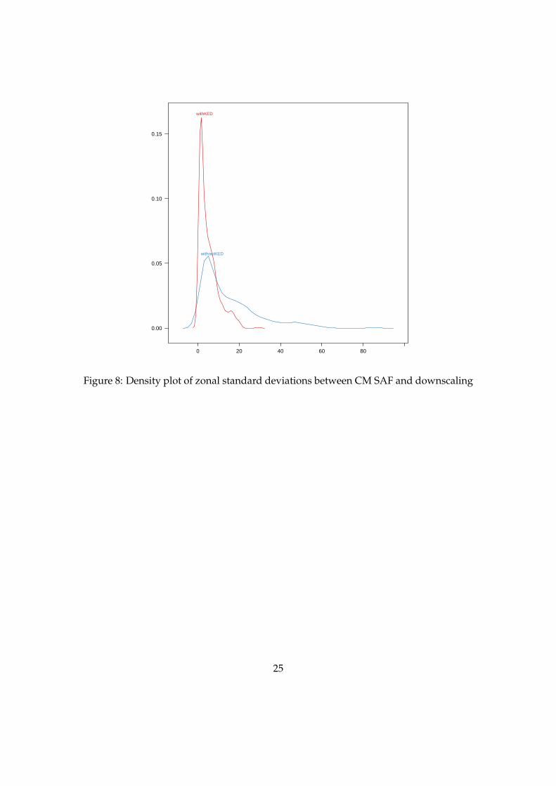
The intrapixel variability due to the downscaling procedure is indicative of the im-portance of the topography as an attenuator of solar irrradiation. As a result, this zonalvariability is higher in pixels with complex topographies and downscaling is more use-ful. Figure 6 shows the relative difference between downscaling with KED and CMSAF. As might be deduced, CM SAF over-estimates GHI in this region by between 11and 22%. Figures 7 and 8 display the standard deviations of the downscaled mapswithin each cell of the original CM SAF raster (0.03x0.03◦). The zonal function fromthe raster library permits this calculation, explaining the intrinsic variability of solarradiation within gross resolution pixels. Consequently, in those pixels with higher stan-dard deviations there will be greater variability. Figure 8 shows how the KED methodsmooths the deviation within pixels and also the range of solar irradiation in the region(Figure 4).

6 Concluding comments

A methodology for downscaling solar irradiation is described and presented using Rsoftware. This methodology is useful for increasing the accuracy and spatial resolution

13

of gross resolution satellite-estimates of solar irradiation.It has been proved that areas whose topography is complex show greater differences

with the original gross resolution data as a consequence of horizon blocking and lowersky-view factors, so downscaling is highly recommended in these areas.

Kriging with external drift with the gstat package has proved very useful in down-scaling solar irradiation when on-ground registers are available and an explanatoryvariable is provided.

This methodology is implemented as an example in the region of La Rioja in north-ern Spain, and striking reductions of annual 46.75% and 43.38% in MAE and RMSEare obtained compared to the original gross resolution database. MBE obtained withdownscaling are lower the threshold value of CM SAF (131.4kWh/m2), proving thehigh influence of topography on solar irradiation.

The high repeatability of this methodology and the reduction in errors obtainedwith annual values might be also very useful in the downscaling of hourly and dailyvalues of solar irradiation and also for different meteorological variables (omitting thesky-view and horizon blocking steps). The code is freely available without restrictionsfor future replications or variations of the study at https://github.com/EDMANSolar/downscaling.

Software information

The results discussed in this paper were obtained in a R session with these characteris-tics:

• R version 2.15.2 (2012-10-26), x86_64-apple-darwin9.8.0

• Locale: es_ES.UTF-8/es_ES.UTF-8/es_ES.UTF-8/C/es_ES.UTF-8/es_ES.UTF-8

• Base packages: base, datasets, graphics, grDevices, grid, methods, parallel,stats,utils

• Other packages: foreign 0.8-51, gstat 1.0-16, hexbin 1.26.0, lattice 0.20-15,latticeExtra 0.6-19, maptools 0.8-14, raster 2.1-16, rasterVis 0.20-01,RColorBrewer 1.0-5, rgdal 0.8-01, solaR 0.33, sp 1.0-8, zoo 1.7-9

• Loaded via a namespace (and not attached): intervals 0.14.0, spacetime 1.0-4,tools 2.15.2, xts 0.9-3

Acknowledgements

We are indebted to the University of La Rioja (fellowship FPI2012) and the ResearchInstitute of La Rioja (IER) for funding parts of this research.

14

References

H. Alsamamra, J. A. Ruiz-Arias, D. Pozo-Vázquez, and J. Tovar-Pescador. A compar-ative study of ordinary and residual kriging techniques for mapping global solarradiation over southern Spain. Agricultural and Forest Meteorology, 149(8):1343 – 1357,2009.

F. Antonanzas-Torres, F. Cañizares, and O. Perpiñán. Comparative assessment of globalirradiation from a satellite estimate model (CM SAF) and on-ground measurements(SIAR): A Spanish case study. Renewable and Sustainable Energy Reviews, 21:248–261,2013.

F. Antonanzas-Torres, A. Sanz-Garcia, F. J. Martínez-de-Pisón and O. Perpiñán-Lamigueiro. Evaluation and improvement of empirical models of global solar ir-radiation: Case study northern Spain. Renewable Energy, 60:604–614, 2013.

F. Antonanzas-Torres, A. Sanz-Garcia, F. J. Martínez-de-Pisón and O. Perpiñán-Lamigueiro. Evaluation and improvement of empirical models of global solar ir-radiation: Case study northern Spain. Renewable Energy, 60:604–614, 2013.

F.J. Batlles, J.L. Bosch, J. Tovar-Pescador, M. Martínez-Durbán, R. Ortega, and I. Mi-ralles. Determination of atmospheric parameters to estimate global radiation in areasof complex topography: Generation of global irradiation map. Energy Conversion andManagement, 49(2):336 – 345, 2008.

J.L. Bosch, F.J. Batlles, L.F. Zarzalejo, and G. López. Solar resources estimation combin-ing digital terrain models and satellite images techniques. Renewable Energy, 35(12):2853 – 2861, 2010.

J. Corripio. Vectorial algebra algorithms for calculating terrain parameters from DEMsand solar radiation modelling in mountainous terrain. International Journal of Geo-graphical Information Science, 17:1–23, 2003.

E. Hay and D.C. Mckay. Estimating solar irradiance on inclined surfaces: a review andassessment of methodologies. International Journal of Solar Energy, 3:203–240, 1985.

T. Hengl. A practical guide to geostatistical mapping. 2009. URL http://spatial-analyst.net/book/.

R. J. Hijmans and J. van Etten. raster: geographic data analysis and modeling, 2013. URLhttp://CRAN.R-project.org/package=raster. R package version 2.1-25.

E. J. Pebesma. Multivariable geostatistics in S: the gstat package. Computers & Geo-sciences, 30:683–691, 2004.

E. Pebesma and B. Graeler. gstat: Spatial and spatio-temporal geostatistical modelling,prediction and simulation, 2013. URL http://CRAN.R-project.org/package=gstat.R package version 1.0-16.

15

E. Pebesma, R. Bivand, B. Rowlingson, and V. Gomez-Rubio. sp: classes and methodsfor spatial data, 2013. URL http://CRAN.R-project.org/package=sp. R package ver-sion 1.0-9.

R. Perez, R. Seals, R. Stewart, A. Zelenka, and V. Estrada-Cajigal. Using satellite-derivedinsolation data for the site/time specific simulation of solar energy systems. SolarEnergy, 53(6):491 – 495, 1994.

O. Perpiñán-Lamigueiro. solaR: Solar radiation and photovoltaic systems with R. Jour-nal of Statistical Software, 50(9):1–32, 8 2012. ISSN 1548-7660. URL http://www.jstatsoft.org/v50/i09.

O. Perpiñán-Lamigueiro. Energía solar fotovoltaica. 2013. URL http://procomun.wordpress.com/documentos/libroesf/.

O. Perpiñán-Lamigueiro and R. J. Hijmans. rasterVis: visualization methods for the rasterpackage, 2013. URL http://CRAN.R-project.org/package=rasterVis. R packageversion 0.20-07.

J. Polo, F. Antonanzas-Torres, J. M. Vindel, and L. Ramirez. Sensitivity of satellite-basedmethods for deriving solar radiation to different choice of aerosol input and models.Renewable Energy, 68:785–792, 2014.

R. Posselt, R.W. Mueller, R. Stöckli, and J. Trentmann. Remote sensing of solar surfaceradiation for climate monitoring — the CM SAF retrieval in international compari-son. Remote Sensing of Environment, 118(0):186 – 198, 2012.

J. Trentmann, C. Träger-Chatterjee, R. Müller, R. Posselt, and R. Stöckli. Meteosat(MVIRI) solar surface irradiance and effective cloud albedo climate data sets. TheCM SAF validation report. Technical report, The EUMETSAT network of satelliteapplication facilities, 2011.

R Development Core Team. R: a language and environment for statistical computing. RFoundation for Statistical Computing, Vienna, Austria, 2013. URL http://www.R-project.org. ISBN 3-900051-07-0.

J. A. Ruiz-Arias, J. Tovar-Pescador, D. Pozo-Vázquez and H. Alsamamra. A compara-tive study of DEM-based models to estimate solar radiation on mountainous terrains.International Journal of Geographical Information Science, 23(8):1049 – 1076, 2009.

J. A. Ruiz-Arias, T. Cebecauer, J. Tovar-Pescador, and M. Šúri. Spatial disaggregationof satellite-derived irradiance using a high-resolution digital elevation model. SolarEnergy, 84(9):1644 – 1657, 2010.

J. Schulz, P. Albert, H.-D. Behr, D. Caprion, H. Deneke, S. Dewitte, B. Dürr, P. Fuchs,A. Gratzki, P. Hechler, R. Hollmann, S. Johnston, K.-G. Karlsson, T. Manninen,R. Müller, M. Reuter, A. Riihelä, R. Roebeling, N. Selbach, A. Tetzlaff, W. Thomas,

16

M. Werscheck, E. Wolters, and A. Zelenka. Operational climate monitoring fromspace: the EUMETSAT satellite application facility on climate monitoring (CM-SAF).Atmospheric Chemistry and Physics, 9(5):1687–1709, 2009.

M. Šúri and J. Hofierka. A new GIS-based solar radiation model and its application forphotovoltaic assessments. Transactions in GIS, 8(2):175 – 190, 2004.

J. M. Vindel, J. Polo and, F. Antonanzas-Torres. Improving daily output of global todirect solar irradiance models with ground measurements. Journal of Renewable andSustainable Energy, 5:063123, 2013.

Database Product Spatial coverage Spatial resolution Temporalcoverage

Temporalresolution

CM SAF SIS ClimateData Set (GHI)

Global 0.25x0.25◦ 1982-2009 Dailymeans

CM SAF SIS ClimateData Set (GHI)

70S-70N, 70W-70E

0.03x0.03◦ 1983-2005 Hourlymeans

CM SAF SID ClimateData Set (BHI)

70S-70N, 70W-70E

0.03x0.03◦ 1983-2005 Hourlymeans

SODA Helioclim 3 v2and v3 (GHI)

66S-66N,66W-66E

5km 2005 15 minutes

SODA Helioclim 3 v2and v3 (GHI)

66S-66N,66W-66E

5km 2005 15 minutes

NREL GHI Moderateresolution

Central andSouth America,Africa, India,East Asia

40x40km 1985-1991 Monthlymeans ofdaily GHI

NASA SSE Global 1x1◦ 1983-2005 Dailymeans

Table 1: Summary of satellite-derivd solar irradiation databases

17

Longitude

Latit

ude

42°N

42.2°N

42.4°N

42.6°N

3°W 2.5°W 2°W

1

2

3

45

6

500 1000 1500 2000

Figure 1: Topographic map of the region analyzed (with elevation in meters) and mete-orological stations considered

# Name Net. Lat.(o) Long.(o)Alt. GHIa

1 Ezcaray SOS 42.33 -3.00 1000 1479

2 Logroño SOS 42.45 -2.74 408 1504

3 Moncalvillo SOS 42.32 -2.61 1495 1329

4 San Roman SOS 42.23 -2.45 1094 1504

5 Ventrosa SOS 42.17 -2.84 1565 1277

6 Yerga SOS 42.14 -1.97 1235 1448

Table 2: Summary of the meteorological stations selected. GHIa stands for the annualGHI in kWh/m2

18

GHI BHI

Disaggregation

GHIdis + BHIdis

DHIdis

Hay & McKay

DHIiso DHIani

Sky View Horizon

DHIiso,down DHIani,down BHIdown

+

GHIdown

GHIground KED

GHIdown,ked

+ −

DEM

Irradiation components

Spatial dissagregation

SVF and horizon shading

KED

Figure 2: Methodology of downscaling: this figure uses red ellipses and lines for datasources, blue ellipses and lines for derived rasters (results), and black rectangles andlines for operations. GHI and BHI stand for global and direct horizontal irradiation,respectively. DHI stands for diffuse horizontal irradiation. Subscripts dis stand fordisaggregated, iso for isotropic, ani for anisotropic, down for downscaled and groundfor measured values. KED and DEM stand for kriging with external drift and digitalelevation model, respectively

19

Longitude

Latit

ude

42°N

42.2°N

42.4°N

42.6°N

3°W 2.5°W 2°W

1500 1550 1600 1650 1700

Figure 3: Annual GHI of 2005 from CM SAF estimates (0.03x0.03◦) in La Rioja (kWh/m2)

20

Longitude

Latit

ude

42°N

42.2°N

42.4°N

42.6°N

3°W 2.5°W 2°W

1200 1250 1300 1350 1400

Figure 4: Annual GHIdown,ked of 2005 (0.03x0.03◦) in La Rioja (kWh/m2)

21

42.0

42.2

42.4

42.6

●

●

●

●

● ●

CM SAF

●

●

●

●●

●

Downscaling and KED

42.0

42.2

42.4

42.6

−3.0 −2.5 −2.0

●

●

●

●●

●

Downscaling

●●

●

●

●

[−0.25,−0.15](−0.15,−0.05](−0.05,0.05](0.05,0.15](0.15,0.25]

Figure 5: Annual relative differences in per one units evaluated with station measure-ments (1-GHIestimated/GHIground). The x and y axis represents the latitude and longitude(o), respectively

GHICMSAF GHIdown,kedMAE 172.62 91.92RMSE 175.02 99.08MBE -172.62 -91.92

Table 3: Summary of testing errors obtained in kWh/m2

22

Longitude

Latit

ude

42°N

42.2°N

42.4°N

42.6°N

3°W 2.5°W 2°W

−0.22 −0.20 −0.18 −0.16 −0.14 −0.12 −0.10

Figure 6: Relative difference of GHIdown,ked and GHIdis (GHIdown,ked/GHIdis -1) in perone units

23

Longitude

Latit

ude

42°N

42.2°N

42.4°N

42.6°N

3°W 2.5°W 2°W

0 10 20 30 40 50 60

Figure 7: Difference of zonal standard deviations (kWh/m2) of GHIdown andGHIdown,KED

24

0.00

0.05

0.10

0.15

0 20 40 60 80

withoutKED

withKED

Figure 8: Density plot of zonal standard deviations between CM SAF and downscaling

25