REAL-TIME SIMULATION OF ROTOR INFLOW USING A

COUPLED FLIGHT DYNAMICS AND FLUID DYNAMICS

SIMULATION

J. Bludau ∗ J. Rauleder † L. Friedmann ‡ M. Hajek �

Institute of Helicopter Technology

Technical University of Munich, 80333 Munich, Germany

In order to predict the rotorcraft motion in the vicinity of objects or their wake, a real-timecapable model is presented. The dynamic in�ow into the rotors was extracted from a real-time Lattice-Boltzmann �uid simulation and fed into a blade element based rotorcraft �ightdynamics code. To represent the in�uence of arbitrary objects on the �ight dynamics, the objectswere modeled by boundary conditions in the Lattice-Boltzmann �uid simulation and updateddynamically in every time step. This two-way coupled simulation enabled the prediction of therotorcraft motion and �ight dynamics in arbitrary situations without prior knowledge of the �ow�eld. To validate the e�ect of objects on the in�ow, the required power in hover and forward�ight in ground e�ect was evaluated. Furthermore, the rotorcraft motion due to a step input inhovering and forward �ight was discussed. The results from the coupled �uid dynamics/�ightdynamics model showed good agreement when compared to a more established reference model,namely the Pitt-Peters in�ow model.

Nomenclature

Acell Area of projection of the cell onto the rotor disk, m2

Aint Area of polygon resulting from intersection, m2

BEM Blade element methodcs Smagorinksy constantcosl Vector of cosine coe�cients of lth order, Nd Cell length in �uid solver, m∆Ψ Halve angle of circular segment, radf Vector of volume force in cell, NfperCell Vector of volume force per cell inside the rotor, NLBM Lattice-Boltzmann methodN Cells per edgelength of cubic domain in the �uid solverNb Number of bladesNharm Number of included harmonicsNin Number of cells fully within the rotorNψ Number of points in circumferential directionNR Number of blade elementsNorth,East,Down Positions of rotorcraft center of gravity in North-East-Down system, mpcg, qcg, rcg Rotation rates of rotorcraft center of gravity in cg system, deg/sPIGE Power in ground e�ect, kWPOGE Power out of ground e�ect, kW

∗ Graduate Student, jakob.bludau@tum.de† Assistant Professor, juergen.rauleder@tum.de‡ Former Research Assistant, friedmann@tum.de� Professor and Department Head, hajek@tum.de

Deutscher Luft- und Raumfahrtkongress 2016DocumentID: 420304

1©2016

Φ,Θ,Ψ Attitudes of rotorcraft center of gravity in North-East-Down system, degr Radial blade coordinate, mR Main rotor radius, mRANS Reynolds-averaged Navier�Stokessinl Vector of sine coe�cients of lth order, Nt Time, sT i Thrustvector of blade i, Nu Vector of in�ow velocities, m/sucg, vcg, wcg Velocities of rotorcraft center of gravity in cg system, m/sxcg, ycg, zcg Coordinates in the body-�xed coordinate system in the center of gravityxlbm, ylbm, zlbm Coordinates in the �uid solver coordinate systemz Height above ground, m

1 INTRODUCTION

Rotorcraft �ight in the vicinity of large objects orin non-uniform and non-stationary �ow conditions ofthe surrounding air are among the most challengingsituations for pilots. As the objects and wakes in�u-ence the rotors, the reaction of the rotorcraft to pilotinputs is altered. This requires the pilot to adapt tothe constantly changing �ight dynamics while beingin high-workload situations. A well known exampleis the take-o� and landing on moving ship decks atquickly changing wind speeds and directions. In orderto be able to train pilots to master such situationssafely and without risk for man and machine, it isinevitable to provide training in �ight simulators.Therefore, a real-time capable simulation of rotor-craft �ight dynamics that captures the in�uence ofarbitrary surroundings and �ow environments on the�ight behavior and handling qualities is necessary.

As the forces of the rotors mainly de�ne therotorcraft's dynamics, the correct calculation of theaerodynamic forces produced by the rotors is ofparticular importance. Therefore, the local angle ofattack along the blades and the velocity relative tothe air is necessary. The resulting lift and drag causethe blades to perform lead-lag and �apping motions,which change the local angle of attack and thereforethe resulting aerodynamic forces. Furthermore, theaerodynamic forces accelerate the air when passingthrough the rotor, inducing a very complex in�owinto the rotors. This in�ow changes the local angle ofattack of the blades. In order to capture the correctrotor dynamics, the angle of attack, blade motion,and forces inside the rotor are needed, which dependstrongly on the in�ow of air. Therefore, the in�ow ismodeled as a function of the aerodynamic forces. Inthis regard one widely used model is the Pitt-Petersdynamic in�ow model [1] which was used as thereference model in the current work.

There are various approaches to enhance modelslike the Pitt-Peters model which assume uniform �owconditions upstream of the rotors and the absenceof objects in the rotor wake. One example is themodel of Gennaretti et al. [2] who used higher-ordercoe�cients to account for the non-uniformity of thein�ow. Nevertheless, these models are not capableof representing the in�uence of arbitrary objectssurrounding the rotorcraft. Other approaches useRANS based computational �uid dynamics to calcu-late the �ow �eld, which enables them to capture thein�uence of nearby objects [3�6]. Unfortunately, thecomputational costs eliminate the real-time capability.Thus, databases with external �ow �eld data haveto be created as a preliminary step. In a similarmanner, experimental data of the �ow �eld can beused although, this limits the validity to reviouslymeasured cases, geometries and �ow conditions.Another recently developed approach used the freevortex wake method on graphic cards in order toachieve real-time capability [7].

In contrast, the presented method used a modi�edversion of the comparably low-resolution �uid dynam-ics solver which was developed in-house at the Tech-nical University of Munich [8]. This solver was cou-pled with a blade element based �ight dynamics code(BEM) to calculate the rotorcraft motion in arbitrary�ight situations using arbitrary boundary conditions.As the in�uence of objects and wakes is transported tothe rotors by the �uid simulation, the resulting e�ectson the rotorcraft motion can be captured by the BEMcode. The resulting thrust was imposed as a volumeforce in the �ow simulation. This two-way couplingenabled the model to capture the dynamic in�uenceof the surroundings of the rotorcraft on its �ight dy-namics and on the produced �ow �eld in real-time; anexample is shown in Fig. 1.

Deutscher Luft- und Raumfahrtkongress 2016

2©2016

Figure 1: Visualization of the �ow �eld aroundthe Bo 105 helicopter hovering above a shipdeck. Colored streamlines used to indicate di-rection and velocity of the �ow.

2 MODELING APPROACH

2.1 Simulation of rotorcaft dynamics

Throughout this paper, the considered rotorcraft wasa MBB Bo 105 helicopter with a total mass of 2500 kgand a main rotor radius of R = 4.92m. The usedBEM code modeled the main rotor as being fullyarticulated, allowing lead-lag, �ap and featheringmotion. The blades were modeled as rigid. In radialdirection each blade was discretized with NR = 8blade elements. These were placed from r

R = 0.223up to r

R = 1 in decreasing distances towards theblade tip, as can be seen in Fig. 2. The sectionof r

R < 0.223 was assumed to be aerodynamicallyneutral and therefore producing neither thrust nordrag. This assumption is valid, because the velocityresulting from the rotation of the blades dominatesthe absolute velocity of the blade element relative tothe air. As this circumferential speed at r

R < 0.223is low compared to the speed at the outer sections ofthe blade, and the blade not having an aerodynamicpro�le, the resulting lift and drag of this section of theblade are comparably small and they were thereforeneglected for simplicity.

In circumferential direction NΨ = 72 positions forthe azimuth Ψ were used. The forces on the blade atthese positions were calculated by interpolating liftand drag from pro�le polars at the blade elements andintegrating over the blade length using the Simpsonrule. The aerodynamic forces of the fuselage andempennage were interpolated from polars similar tothe forces of the blades.

As the rotors were represented by actuator disks inthe �uid simulation, the thrust at every radial and cir-cumferential position inside the disk was needed. In

0.2 0.4 0.6 0.8 10

2

4

6

r/R

Index

ofbladeelem

ent

Figure 2: Radial position of the blade elementsused in the BEM code.

order to provide this, the BEM code turned the ro-tor until the blade motion and forces were steady overthe revolution of the rotor. By this, the forces of theblades were no longer dependent on the position andvelocity of the blade at the beginning of the timestep,and the thrust that had to be imposed on the actu-ator disk was extracted. At low frequency inputs orvariations in the in�ow into the rotors, this assump-tion is valid as the blade motion adjust after aboutone revolution, which is very fast compared to the re-action of the rotorcraft [9]. Unfortunately, this steadystate assumption alters the rotor dynamic behavior atfrequencies in the range of the rotor's rotational fre-quency, as the blades do not reach stationary motionand forces per revolution. Nevertheless, it is shown inSec. 3.2 that for the imposed step inputs in combina-tion with an actuator disk to represent the rotors, thesteady state assumption is valid.

2.2 Numerical setup of the �uid solver

The used �uid dynamics solver is based on the Lattice-Boltzmann method (LBM). Therefore, the Boltzmannequation is approximated using discrete cells contain-ing particle distributions and a collision operator to ac-count for particle interactions which results in a weaklycompressible �uid behavior [10,11]. For details on thesolver see Ref. [8]. It was embedded in a frameworkwhich dynamically generated boundary conditions inorder to represent nearby obstacles [8]. This enabledthe real-time calculation of the �ow �eld even whenthe rotorcraft or the objects were in motion.The �uid domain in the LBM solver was cubic with

an edge length of 4R with R being the main rotorradius. Inside this domain the main rotor was locatedone R from the top. This left 3R below the rotor tocapture the ground e�ect which becomes negligible atheights larger than 3R above ground [12]. A schematicview of the domain and grid is depicted in Fig. 3.The resolution N of the simulation was de�ned

Deutscher Luft- und Raumfahrtkongress 2016

3©2016

xcgycgzcg

xlbmzlbm

ylbm klbm

ilbm

jlbm

Figure 3: Fluid domain with a grid of N = 4, co-ordinate system of the center of gravity, cg andcoordinate system and grid indices of the LBMsolver, lbm. For simplicity cell edges inside thedomain are not shown. Adapted from [8].

as the number of cells per edge length of the cubicdomain. This resulted in a cell length d = 4R

N . Forthe MBB Bo 105 helicopter with R = 4.92 m the celllenghts are listed in Ref. [8].

Because of the grid being �xed to the helicopter'scenter of gravity, it was moved according to therotorcraft. In order to account for the movement,an Eulerian-Lagrangian approach as described byMeldi [13] was used. The rotorcraft's fuselage wasmodeled by wall boundary conditions equal to otherobjects in the �ow �eld, as described by Friedmann [8].Furthermore, the outer cells of the domain whichwere not used to model objects by wall boundaryconditions, had to express a far�eld boundary. Toachieve this, impedance based boundary conditionswere used, as described by Schla�er [14]. In orderto keep the solver stable when using the impedanceboundary conditions, a Smagorinsky turbulencemodel with a Smagorinksy constant of cs = 0.075 wasused in all current simulations.

In contrast to the fully articulated rotor in theBEM, the rotor in the LBM was represented by onestationary layer of cells representing an actuatordisk. This disk approximates a rotor with an in�nitenumber of blades and imposes a force at every radialand circumferential position. As the range of r/Rof the blade elements in the BEM was 0.233 ... 1,the area of the rotor was formed by the rotor disk

area minus a circle with 0.223R radius in the center.As the Cartesian grid was not able to adequatelyrepresent this rotor due to the low resolution whichleads to large cell sizes, all cells that were not includedcompletely inside the rotor had to be treated ina special way. As the grid was aligned with therotor, the projection of the cells onto the rotor diskwere squares. By intersecting the correspondingcells with a polygon representation of the rotor, thefraction of the cell that lay within the rotor wascalculated. To identify the cells that were not fullywithin the disk, two circles with Ri = R − 0.5

√2d

and Ro = R + 0.5√

2d, concentric with the rotor diskwere used. All cells, whose center point lay betweenthese two circles, did not lie fully within the rotor,and had to be intersected with the disk. To reducethe computational cost, the implemented algorithmcalculated the azimuth position of the cell's vertexand formed a circular segment using the angle ∆Ψ asit is shown schematically in green in Fig. 4.

∆Ψ = tan−1(√2d

R

)(1)

R

Ri

Ro

∆Ψ∆Ψ

Figure 4: Schematic view of the intersection ofa cell with a convex six-sided polygon (green)representing a segment of the circular disk.Intersection-points and -area in red.

This polygon was intersected with the cell using thelinear algorithm of O'Rourke [15]. The area of theresulting polygon was calculated by the Shoelace for-mula [16], and a volume force proportional to the areainside the circular disk was imposed on the cell:

f =AintACell

fperCell(2)

where f is the volume force, Aint the area of theintersection, ACell the area of the cell and fperCell

the force acting per cell. To induce the force in theLBM, the scheme of Guo [17] was used. Due to theapproximation of the circular disk as convex polygon,the resulting area of all cells within the rotor and

Deutscher Luft- und Raumfahrtkongress 2016

4©2016

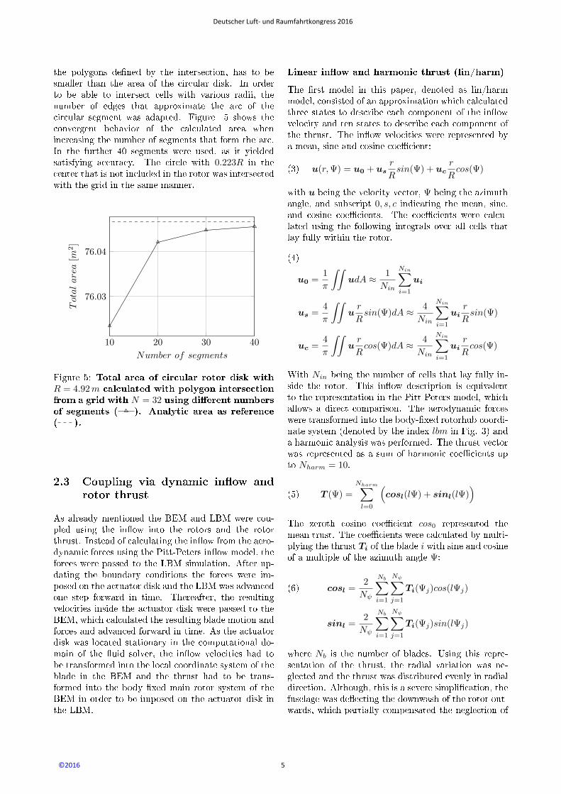
the polygons de�ned by the intersection, has to besmaller than the area of the circular disk. In orderto be able to intersect cells with various radii, thenumber of edges that approximate the arc of thecircular segment was adapted. Figure 5 shows theconvergent behavior of the calculated area whenincreasing the number of segments that form the arc.In the further 40 segments were used, as it yieldedsatisfying accuracy. The circle with 0.223R in thecenter that is not included in the rotor was intersectedwith the grid in the same manner.

10 20 30 40

76.03

76.04

Number of segments

Totalarea[m

2]

Figure 5: Total area of circular rotor disk withR = 4.92m calculated with polygon intersectionfrom a grid with N = 32 using di�erent numbersof segments ( ). Analytic area as reference( ).

2.3 Coupling via dynamic in�ow and

rotor thrust

As already mentioned the BEM and LBM were cou-pled using the in�ow into the rotors and the rotorthrust. Instead of calculating the in�ow from the aero-dynamic forces using the Pitt-Peters in�ow model, theforces were passed to the LBM simulation. After up-dating the boundary conditions the forces were im-posed on the actuator disk and the LBM was advancedone step forward in time. Thereafter, the resultingvelocities inside the actuator disk were passed to theBEM, which calculated the resulting blade motion andforces and advanced forward in time. As the actuatordisk was located stationary in the computational do-main of the �uid solver, the in�ow velocities had tobe transformed into the local coordinate system of theblade in the BEM and the thrust had to be trans-formed into the body �xed main rotor system of theBEM in order to be imposed on the actuator disk inthe LBM.

Linear in�ow and harmonic thrust (lin/harm)

The �rst model in this paper, denoted as lin/harmmodel, consisted of an approximation which calculatedthree states to describe each component of the in�owvelocity and ten states to describe each component ofthe thrust. The in�ow velocities were represented bya mean, sine and cosine coe�cient:

u(r,Ψ) = u0 + usr

Rsin(Ψ) + uc

r

Rcos(Ψ)(3)

with u being the velocity vector, Ψ being the azimuthangle, and subscript 0, s, c indicating the mean, sine,and cosine coe�cients. The coe�cients were calcu-lated using the following integrals over all cells thatlay fully within the rotor.

u0 =1

π

∫∫udA ≈ 1

Nin

Nin∑i=1

ui

(4)

us =4

π

∫∫ur

Rsin(Ψ)dA ≈ 4

Nin

Nin∑i=1

uir

Rsin(Ψ)

uc =4

π

∫∫ur

Rcos(Ψ)dA ≈ 4

Nin

Nin∑i=1

uir

Rcos(Ψ)

With Nin being the number of cells that lay fully in-side the rotor. This in�ow description is equivalentto the representation in the Pitt-Peters model, whichallows a direct comparison. The aerodynamic forceswere transformed into the body-�xed rotorhub coordi-nate system (denoted by the index lbm in Fig. 3) anda harmonic analysis was performed. The thrust vectorwas represented as a sum of harmonic coe�cients upto Nharm = 10.

T (Ψ) =

Nharm∑l=0

(cosl(lΨ) + sinl(lΨ)

)(5)

The zeroth cosine coe�cient cos0 represented themean trust. The coe�cients were calculated by multi-plying the thrust Ti of the blade i with sine and cosineof a multiple of the azimuth angle Ψ:

cosl =2

Nψ

Nb∑i=1

Nψ∑j=1

Ti(Ψj)cos(lΨj)(6)

sinl =2

Nψ

Nb∑i=1

Nψ∑j=1

Ti(Ψj)sin(lΨj)

where Nb is the number of blades. Using this repre-sentation of the thrust, the radial variation was ne-glected and the thrust was distributed evenly in radialdirection. Although, this is a severe simpli�cation, thefuselage was de�ecting the downwash of the rotor out-wards, which partially compensated the neglection of

Deutscher Luft- und Raumfahrtkongress 2016

5©2016

the radial distribution of the thrust. Figure 6 showsthe imposed thrust in z-direction in each cell over theradial coordinate of the blade at azimuth Ψ = 90 degin hover. At the inner and outer boundary of the ro-tor disk, the polygon intersection of the rotor withthe grid, which is described by Eqn. 2, reduced theimposed thrust. Furthermore, the z-component of thelinearized velocity, wich was sent to the BEM after thelinearization is shown. For comparison the positionsof the blade elements in the BEM are included.

0 0.2 0.4 0.6 0.8 1 1.213

13.1

13.2

13.3

13.4

r/R

uzm s

0

0.5

1

1.5·103

Tz[N

]

Figure 6: Values of velocity( ) sent to theBEM and thrust( ) imposed in the LBM overthe radial coordinate using the lin/harm modelin hover at Ψ = 90 deg. Positions of blade el-ements in BEM marked by ( ), cell verticesmarked by ( )

Local in�ow and local thrust (loc/loc)

The second model, denoted as loc/loc model, usedthe local values of the velocity in each cell to calculatethe total velocity of the blade element relative tothe air. Therefore, all cells within the rotor diskwere passed to the BEM. For each blade element,the velocity of the nearest cell was imposed as in�owvelocity. After superimposing the velocities resultingfrom the blade motion, the aerodynamic forces in allblade elements at all circumferential positions werecalculated and sent to the LBM. An example of theresulting distribution of the velocity and thrust inhover is shown in Fig. 7 for an azimuth position ofΨ = 90 deg. For convenience the positions of theblade elements in the BEM are included. As for thelin/harm model, the polygon intersection of the rotorwith the grid reduces the imposed thrust in cellsintersecting with the boundary of the rotor.

After receiving the local forces at all circumferentialpoints and blade elements from the BEM, the valueof the blade element nearest to the center of each cellwas selected to be imposed as volume force on the

�uid. As this selection process did not conserve thetotal thrust, the thrust in all cells was scaled by afactor. This factor resulted from the mean of eachcomponent of the force that was calculated in theBEM, divided by the sum of the component of theforce imposed in all cells that lay inside or intersectedwith the rotor. By this measure, it was ensured thatthe BEM and LBM used the same thrust values.

0 0.2 0.4 0.6 0.8 1 1.2

0

5

10

15

r/R

uz[ms]

0

1

2

·103

Tz[N

]

Figure 7: Cell values of velocity( ) andthrust( ) of the loc/loc model over the ra-dial coordinate in hover at Ψ = 90 deg. Positionsof blade elements in BEM marked by ( ), cellvertices marked by ( )

Calculation of trimmed state

Independent of the used model to describe in�owand thrust, the model was trimmed using a trimcalculated by the Pitt-Peters model as initial value.To ensure that the �ow �eld was fully developed, theLBM was given 1000 time steps with the calculatedthrust. At the resolution of N = 32 this correspondedto 2.78s. With a downwash velocity of approximately11ms this ensured that the free stream reached thefar-�eld boundary, even if at zlbm = −3R a wallboundary de�ected the stream.

Thereafter, the model was trimmed using the cou-pled LBM/BEM with the �ow �eld from the previoustrim as initial condition. As it had to be ensured thatthe �uid solution was stationary, the LBM was ad-vanced for 1000 time steps in each trim step followingthe same procedure as previously discussed. A trimwas found if the longitudinal and lateral residuals ofthe forces were below 50 N, the vertical below 100 N,the residual of the rolling moment below 50 Nm, andthe residuals of pitching and yawing moments below100 Nm. This algorithm is similar to the one used inRef. [3].Throughout this article, the tail rotor of the Bo 105

Deutscher Luft- und Raumfahrtkongress 2016

6©2016

was not modeled using the coupled approach. Due toits small size, it would have been resolved by only fourcells at a resolution of N = 32. Instead, the in�owto the tail rotor was calculated using the Pitt-Petersmodel. Nevertheless, as both rotors are inside thesame computational domain, the model is, in princi-ple, able to capture rotor-rotor interaction when bothrotors are su�ciently resolved.

3 RESULT AND DISCUSSION

In order for the presented two-way coupled models tobe valid, they have to be able to correctly depict the ro-torcraft's �ight dynamics even when arbitrary objectsin�uence the �ow �eld around the helicopter. Fur-thermore, they must show convergent behavior if theresolutions of the LBM and BEM are increased. Asa �rst step, the behavior in stationary forward �ightand in ground e�ect was assessed. Furthermore, thedynamic response of the models is compared to thePitt-Peters reference model.

3.1 Stationary forward �ight and in�u-

ence of ground e�ect

In trimmed forward �ight out of ground e�ect, bothpresented models showed good agreement concerningthe required power which is shown in Fig. 8. Forthe lin/harm model the induced power is calculatedfrom the mean thrust in z-direction, T̄z, and the meaninduced velocity in z-direction, v̄z, of all cells thatare fully inside the rotor. For the loc/loc model theinduced power was calculated by summing the localthrust times the induced velocity over all cells thatlay within or intersected with the rotor. Both mod-els showed good agreement with the reference modelconcerning the induced power.

0 20 40 600

200

400

600

ugc [ms ]

P[kW

]

Figure 8: Required power ( ) and inducedpower( ) of the lin/harm ( ), loc/loc( ), and Pitt-Peters model ( )

Concerning the necessary inputs for the trimmedforward �ight states, shown in Fig. 9, both pre-sented models showed good agreement with the refer-ence model concerning the collective and pedal input.In contrast to the power at forward speeds below 20 m

s ,both presented models showed deviations from the ref-erence model in the longitudinal and lateral input. Atspeeds above 20 m

s the inputs of the presented and thereference model converged, although, the di�erence inthe lateral input between the presented models andthe reference did not fall below 5%.

0 20 40 60

40

60

80

100

ugc [ms ]

Input[%

]

Figure 9: Collective( ), pedal( ),lateral( ), and longitudinal input( )of the lin/harm ( ), loc/loc ( ), andPitt-Peters model ( ) in trimmed forward�ight

When hovering in heights of z < 3R the ground in-�uences the rotor thrust at a given power [9,12]. Thisis equal to a reduction in the induced power at a giventhrust [12, 18]. Among others, Cheeseman and Ben-nett [19] or Johnson [9] proposed models to accountfor the power reduction while hovering in ground ef-fect. Neglecting blade loading e�ects, the Cheesemanmodel reduces to:

PIGEPOGE

|T=const = 1− 1

16

R

z

2

(7)

The model of Johnson describes the power reductionwith use of an exponential function:

PIGEPOGE

|T=const =1

1 + e−2z/R(8)

In order to calculate the power reduction in grounde�ect for the presented models, POGE and PIGE intrimmed hover were extracted for various heightsabove ground. For z > 3R, POGE = 480.9 kW andPOGE = 458.0 kW were obtained for the lin/harmand loc/loc model, which correlated well to thePOGE = 464.7 kW obtained using the dynamic in�owmodel of Pitt and Peters. The same was true for the

Deutscher Luft- und Raumfahrtkongress 2016

7©2016

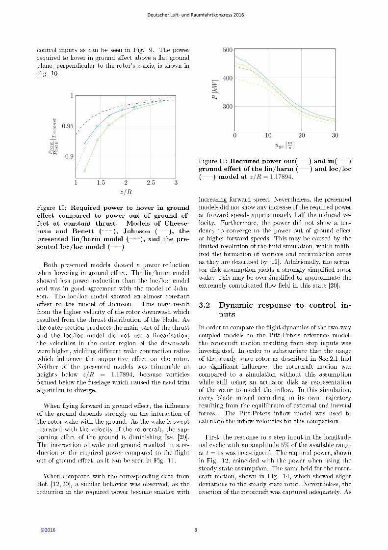
control inputs as can be seen in Fig. 9. The powerrequired to hover in ground e�ect above a �at groundplane, perpendicular to the rotor's z-axis, is shown inFig. 10.

1 1.5 2 2.5 3

0.9

0.95

1

z/R

PIGE

POGE| T

=const

Figure 10: Required power to hover in grounde�ect compared to power out of ground ef-fect at constant thrust. Models of Cheese-man and Benett ( ), Johnson ( ), thepresented lin/harm model ( ), and the pre-sented loc/loc model ( )

Both presented models showed a power reductionwhen hovering in ground e�ect. The lin/harm modelshowed less power reduction than the loc/loc modeland was in good agreement with the model of John-son. The loc/loc model showed an almost constanto�set to the model of Johnson. This may resultfrom the higher velocity of the rotor downwash whichresulted from the thrust distribution of the blade. Asthe outer section produces the main part of the thrustand the loc/loc model did not use a linearisation,the velocities in the outer region of the downwashwere higher, yielding di�erent wake contraction ratioswhich in�uence the supportive e�ect on the rotor.Neither of the presented models was trimmable atheights below z/R = 1.17894, because vorticiesformed below the fuselage which caused the used trimalgorithm to diverge.

When �ying forward in ground e�ect, the in�uenceof the ground depends strongly on the interaction ofthe rotor wake with the ground. As the wake is sweptrearward with the velocity of the rotorcraft, the sup-porting e�ect of the ground is diminishing fast [20].The interaction of wake and ground resulted in a re-duction of the required power compared to the �ightout of ground e�ect, as it can be seen in Fig. 11.

When compared with the corresponding data fromRef. [12, 20], a similar behavior was observed, as thereduction in the required power became smaller with

0 10 20 30

300

400

500

ugc [ms ]

P[kW

]

Figure 11: Required power out( ) and in( )ground e�ect of the lin/harm ( ) and loc/loc( ) model at z/R = 1.17894.

increasing forward speed. Nevertheless, the presentedmodels did not show any increase of the required powerat forward speeds approximately half the induced ve-locity. Furthermore, the power did not show a ten-dency to converge to the power out of ground e�ectat higher forward speeds. This may be caused by thelimited resolution of the �uid simulation, which inhib-ited the formation of vortices and recirculation areasas they are described by [12]. Additionally, the actua-tor disk assumption yields a strongly simpli�ed rotorwake. This may be oversimpli�ed to approximate theextremely complicated �ow �eld in this state [20].

3.2 Dynamic response to control in-

puts

In order to compare the �ight dynamics of the two-waycoupled models to the Pitt-Peters reference model,the rotorcraft motion resulting from step inputs wasinvestigated. In order to substantiate that the usageof the steady state rotor as described in Sec.2.1 hadno signi�cant in�uence, the rotorcraft motion wascompared to a simulation without this assumptionwhile still using an actuator disk as representationof the rotor to model the in�ow. In this simulation,every blade moved according to its own trajectoryresulting from the equilibrium of external and inertialforces. The Pitt-Peters in�ow model was used tocalculate the in�ow velocities for this comparison.

First, the response to a step input in the longitudi-nal cyclic with an amplitude 5% of the available rangeat t = 1s was investigated. The required power, shownin Fig. 12, coincided with the power when using thesteady state assumption. The same held for the rotor-craft motion, shown in Fig. 14, which showed slightdeviations to the steady state rotor. Nevertheless, thereaction of the rotorcraft was captured adequately. As

Deutscher Luft- und Raumfahrtkongress 2016

8©2016

a consequence, the simpli�cation of a steady state ro-tor was considered to be valid for the given �ight con-dition.

0 1 2 3 4 5

420

440

460

480

Time[s]

Pow

er[kW

]

Figure 12: Required power due to a step inputin the longitudinal control in trimmed hover.Amplitude of the step input 5% of the avail-able input range at t = 1s. Pitt-Peters modelwith steady state rotor ( ) and full blade tra-jectory ( ). Lin/harm( ) and loc/loc(model using N = 32.

Concerning the required power of the rotorcraftshown in Fig. 12, both presented models overpre-dicted the power consumption in trimmed hover.When analyzing the rotorcraft motion in hover,shown in Fig. 14, a behavior similar to the referencemodel was observed for the velocities ucg, and wcgand the rotation rates pcg, qcg. The yawing rate rcgshowed signi�cant deviations from the reference modelstarting at t ≈ 3 s and it did not follow the trendsof the reference model. The velocity vcg showed anopposite tendency when compared to the referencemodel which resulted in a wrong position. However,the remaining attitudes and positions were found tobe in good agreement with the reference model.

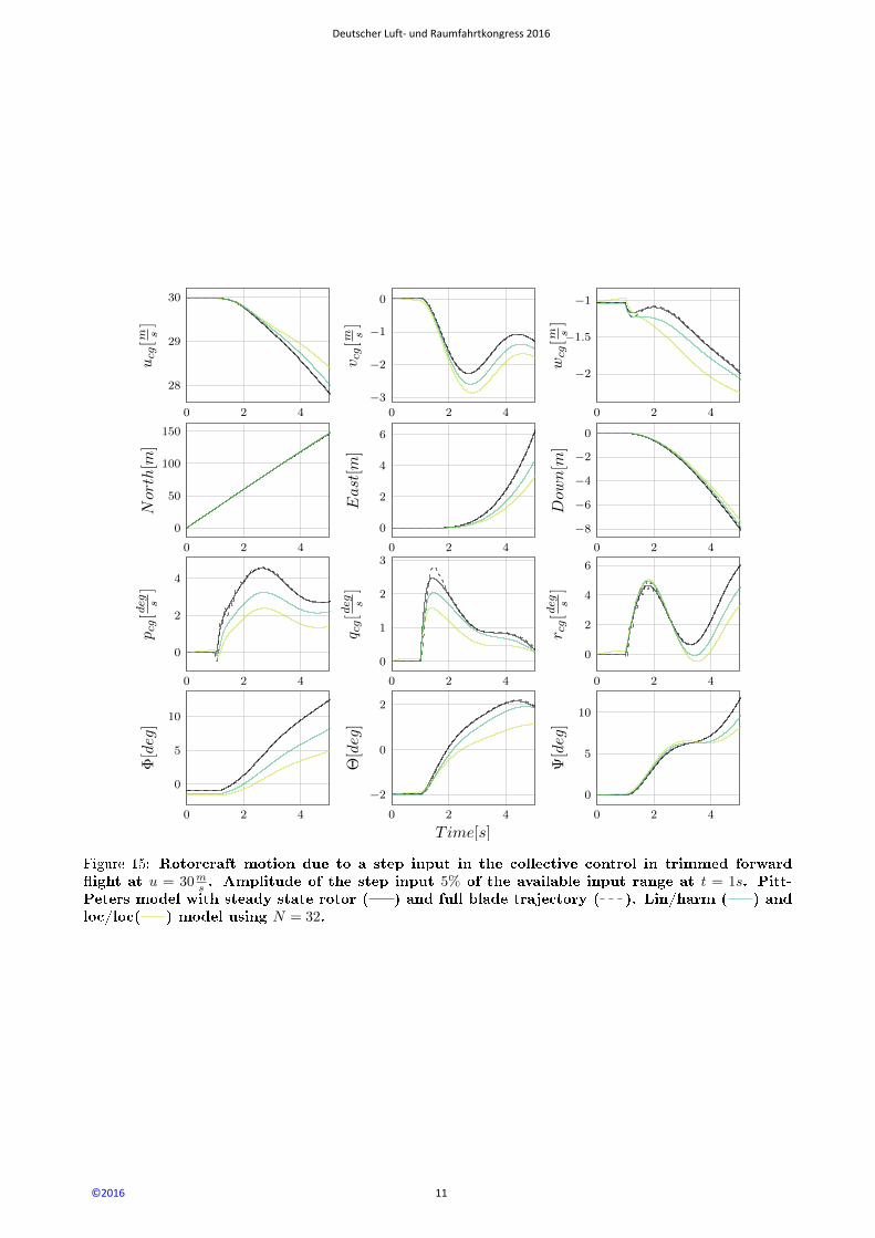
As the second test case, the rotorcraft was trimmedat a forward velocity of ucg = 30 m

s and a step inputin the collective of 5% of the available input rangewas imposed at t = 1s. The required power is shownin Fig. 13. In order to show the validity of assuminga steady state rotor in the given �ight condition, therequired power was compared to the simulation whenusing full blade trajectories. After the step input,the required power was subject to fading oscillationswhen the blade trajectory was taken into account. Asthe step input in the collective caused all blades to�ap with high amplitudes, lift and drag varied andcaused these oscillations in the power required. Whenusing the steady state rotor, the excessive �appingof the blades was not present and, therefore, therewere no oscillations in the required power in this case.However, the mean power during the oscillations was

equal to the power predicted by the steady state rotorsimulation. After approximately 3s the damping ofthe blades due to the aerodynamic and centrifugalforces has eliminated the oscillations. Despite thedi�erent power requirements without it, the steadystate assumption was supported by the rotorcraftmotion. The rotorcraft's response was independent ofthe use of steady state rotors as can be seen in Fig.15. Therefore, the assumption of steady state rotorswas considered valid when analyzing the rotorcraftmotion in the current operating conditions.

0 1 2 3 4 5200

250

300

Time[s]

Pow

er[kW

]

Figure 13: Required power due to a step input inthe collective control in trimmed forward �ightat u = 30ms . Amplitude of the step input 5%of the available input range at t = 1s. Pitt-Peters model with steady state rotor ( ) andfull blade trajectory ( ). Lin/harm( ) andloc/loc( ) model using N = 32.

Concerning the rotorcraft motion, the velocities ucg,vcg and wcg, and the rates pcg, qcg, and rcg showedgood agreement with the reference model. Althoughthe amplitudes of the presented models were underes-timated when compared to the reference model, theyshowed good qualitative agreement, as all velocitiesand rates show the same trends as the reference model.

Deutscher Luft- und Raumfahrtkongress 2016

9©2016

0 2 4

0

2

4

6

8

ucg[ms]

0 2 4

0

1

v cg[ms]

0 2 4

−2

−1

0

wcg[ms]

0 2 4

0

5

10

North[m

]

0 2 4

0

1

2

East[m

]

0 2 4

0

0.5

1

1.5

Dow

n[m

]

0 2 4

0

5

pcg[d

eg s]

0 2 4

−5

0

q cg[d

eg s]

0 2 4

−1

0

1r c

g[d

eg s]

0 2 4

−5

0

5

10

Φ[deg]

0 2 4

−20

−10

0

Time[s]

Θ[deg]

0 2 4

0

1

2

3

Ψ[deg]

Figure 14: Rotorcraft motion due to a step input in the longitudinal control in trimmed hover.Amplitude of the step input 5% of the available input range at t = 1s. Pitt-Peters model withsteady state rotor ( ) and full blade trajectory ( ). Lin/harm ( ) and loc/loc ( ) modelusing N = 32.

Deutscher Luft- und Raumfahrtkongress 2016

10©2016

0 2 4

28

29

30

ucg[ms]

0 2 4

−3

−2

−1

0

v cg[ms]

0 2 4

−2

−1.5

−1

wcg[ms]

0 2 4

0

50

100

150

North[m

]

0 2 4

0

2

4

6

East[m

]

0 2 4

−8

−6

−4

−2

0

Dow

n[m

]

0 2 4

0

2

4

pcg[d

eg s]

0 2 4

0

1

2

3

q cg[d

eg s]

0 2 4

0

2

4

6r c

g[d

eg s]

0 2 4

0

5

10

Φ[deg]

0 2 4

−2

0

2

Time[s]

Θ[deg]

0 2 4

0

5

10

Ψ[deg]

Figure 15: Rotorcraft motion due to a step input in the collective control in trimmed forward�ight at u = 30ms . Amplitude of the step input 5% of the available input range at t = 1s. Pitt-Peters model with steady state rotor ( ) and full blade trajectory ( ). Lin/harm ( ) andloc/loc( ) model using N = 32.

Deutscher Luft- und Raumfahrtkongress 2016

11©2016

4 CONCLUSIONS AND OUT-

LOOK

The ability of the presented real-time capable, two-way coupled �uid dynamics/�ight dynamics modelsto correctly predict the in�uence of a ground planeon the rotorcraft's power in hover was investigated.The results correlated well in power and controls forstationary forward �ight and predicted the grounde�ect in both hover and forward �ight. The dynamicreactions to step inputs in trimmed �ight were foundto be in good agreement with the reference model.This was the �rst step to validate and enhance themodels to be used for piloted simulations in pilottraining facilities. Nevertheless, convergence behaviorneeds to be investigated along with detailed validationof the resulting dynamic in�ow.

The shown results were obtained in real-time usinga Nvidia GeForce 980 Ti for the �ow computationsby the LBM solver. As the time required by the LBMsolver dominated the computational time necessary forone time step, doubling the resolution while preservingthe real-time capability will require roughly 24 timesthe computational power. Nevertheless, increasing thespatial resolution is indispensable in order to be able tocouple the tail rotor in the same manner as it was donefor the main rotor to include rotor-rotor interactionphenomena. Furthermore, the LBM solver's ability tocapture the in�uence of the fuselage and surroundingobjects will be enhanced as �ner approximations ofthe geometries are possible. Because a single graph-ics card is not able to provide the required computa-tional power, e�cient, distributed computation strate-gies will be explored. An increased resolution will alsopermit to use individual blades in the LBM insteadof an actuator disk. These measures are expected toenhance the dynamics of the BEM and allow betterrepresentations of the rotor wake.

References

[1] Pitt, D. M., and Peters, D. A. Theoreticalpredictions of dynamic-in�ow derivatives. Vertica5 (1981), 21�34.

[2] Gennaretti, M., Gori, R., Cardito, F.,

Serafini, J., and Bernadini, G. A space-timeaccurate �nite-state in�ow model for aeroelasticapplications. 72nd Annual Forum of the Ameri-

can Helicopter Society (2016).

[3] Oruc, I., Horn, J. F., Polsky, S., Shipman,J., and Erwin, J. Coupled �ight dynamics andcfd simulations of the helicopter/ship dynamic in-terface. 71st Annual Forum of the American He-

licopter Society (2015).

[4] Polsky, S., Wilinson, C. H., Nichols, J.,

Ayers, D., Mercado-Perez, J., and Davis,

T. S. Development and application of the safeditool for virtual dynamic interface ship airwakeanalysis. AIAA SciTech (2016).

[5] Amsallem, D., Cortial, J., and Farhat, C.

Towards real-time cfd-based aeroelastic computa-tions using a database of reduced-order informa-tion. AIAA Journal Vol. 48 (2010).

[6] Owen, I., and Padfield, G. P. Integrating cfdand piloted simulation to quantify ship-helicopteroperating limits. Aeronautical Journal (2006).

[7] Rubenstein, G., Moy, D. M., Sridharan, A.,

and Chopra, I. A python-based framework forreal-time simulation using comprehensive analy-sis. 72nd Annual Forum of the American Heli-

copter Society (2016).

[8] Friedmann, L., Ohmer, P., and Hajek, M.

Real-time simulation of rotorcraft downwash inproximity of complex obstacles using grid-basedapproaches. 70th Annual Forum of the American

Helicopter Society (2014).

[9] Johnson, W. Helicopter Theory, 2nd ed. DoverPublications, New York, 1994.

[10] Hänel, D. Molekulare Gasdynamik, 1st ed.Springer-Verlag, Berlin Heidelberg, 2004.

[11] Wolf-Gladrow, D. A. Lattice-Gas Cellular

Automata and Lattice Boltzmann Models - An In-

troduction, 1st ed. Springer-Verlag, Berlin Heidel-berg, 2005.

[12] Leishman, J. Principles of Helicopter Aerody-

namics, 2nd ed. Cambridge University Press, NewYork, 2008.

[13] Meldi, M., Vergnault, E., and Sagaut, P.

An arbitrary lagrangian-eulerian approach for thesimulation of immersed moving solids with latticeboltzmann method. Journal of Computational

Physics 235 (2013), 182�198.

[14] Schlaffer, M. Non-Re�ecting Boundary Con-

ditions for the Lattice Boltzmann Method. PhDthesis, Technical University of Munich, 2013.

[15] O'Rourke, J., Chien, C.-B., Olson, T., andNaddor, D. A new linear algorithm for inter-secting convex polygons. Computer Graphics andImage Processing 19 (1982), 384�391.

[16] Braden, V. The surveyor's area formula. The

College Mathematics Journal 17 (1986).

[17] Guo, Z., Zheng, C., and Shi, B. Discrete lat-tice e�ects on he forcing term in the lattice boltz-mann method. Physical Review E 65 (1973).

Deutscher Luft- und Raumfahrtkongress 2016

12©2016

[18] Khromov, V., and Rand, O. Ground e�ectmodeling for rotary-wing simulation. 26th In-

ternational Congress of the Aeronautical Sciences

(2008).

[19] Cheeseman, I., and Bennett, W. The e�ectof the ground on a helicopter rotor in forward�ight. ARC R&M 3021 (1955).

[20] Chen, R. T. N. A survey of nonuniform in�owmodels for rotorcraft �ight dynamics and con-trol applications. 15th European Rotorcraft Fo-

rum (1989).

Deutscher Luft- und Raumfahrtkongress 2016

13©2016