Download (11MB) - City Research Online - City University
236
City, University of London Institutional Repository Citation: Zhao, Weizhong (2011). Optical fibre high temperature sensors and their applications. (Unpublished Doctoral thesis, City University London) This is the unspecified version of the paper. This version of the publication may differ from the final published version. Permanent repository link: http://openaccess.city.ac.uk/1190/ Link to published version: Copyright and reuse: City Research Online aims to make research outputs of City, University of London available to a wider audience. Copyright and Moral Rights remain with the author(s) and/or copyright holders. URLs from City Research Online may be freely distributed and linked to. City Research Online: http://openaccess.city.ac.uk/ [email protected] City Research Online
Transcript of Download (11MB) - City Research Online - City University

City, University of London Institutional Repository
Citation: Zhao, Weizhong (2011). Optical fibre high temperature sensors and their applications. (Unpublished Doctoral thesis, City University London)
This is the unspecified version of the paper.
This version of the publication may differ from the final published version.
Permanent repository link: http://openaccess.city.ac.uk/1190/
Link to published version:
Copyright and reuse: City Research Online aims to make research outputs of City, University of London available to a wider audience. Copyright and Moral Rights remain with the author(s) and/or copyright holders. URLs from City Research Online may be freely distributed and linked to.
City Research Online: http://openaccess.city.ac.uk/ [email protected]
City Research Online

Optical fibre high temperature sensors
and their applications
By
Weizhong Zhao
Thesis submitted for the degree of
Doctor of Philosophy
City University London
School of Engineering and Mathematical Sciences
Northampton Square, London EC1V 0HB
July 2011


Acknowledgements
I
Acknowledgements
It would be definitely impossible to finish the work presented in this thesis without the
enormous help and support from many individuals and institutions.
In particular, I’d like to express my deepest gratitude toward Professor Kenneth T.V.
Grattan, the chief supervisor of my thesis, and professor Tong Sun, the co-supervisor.
Their valuable suggestions and constant observations helped me to move forward to the
direction of research and to achieve this goal. They also supported financially to my
research by permitting me materials and equipment. I thank them for their efforts.
Many thanks should be given to Dr. Zhiyi Zhang. His comprehensive investigation in
the field of fluorescence-based fibre thermometry has set a solid foundation to the
continued work.
Many thanks to Professor Yonghang Shen, Zhejiang University, China, for his
supporting and cooperating in many of this work, particularly in preparing the special
fibres for high temperature gratings.
Many thanks to, Dr. Suchanda Pal, Dr. Jahnal Mandal, Dr. Jackson Yeo, Dr. T.
Venugupalan, Miss Shuying Chen and all the guys in Measurement and Instrumentation
Centre of City University, London. Their kind assistance let me spend smoothly the years
of study at City University.
Finally, I should thank my parents and in-laws, my wife and my daughters. Without their
self-giving contributions, it would be impossible for me to complete this thesis. I do owe
them a lot.

II

Declaration
III
Declaration
I declare that the work presented in this thesis, except those specifically declared, is
all my own work carried out and finished at The City University London

Optical fibre high temperature sensors and their applications
IV
Copyright declaration
The author accepts the fact of discretion to the City University Librarian to allow the
thesis to be copied in whole or in part without the prior written consent to the author.
This thesis may be made available for consultation within the University library and
may be photocopied only single copies or lent to other libraries for the study purpose

Abstract
V
Abstract
Fibre-optic sensors based on different schemes, have grown rapidly since its
concept was first discussed decades ago. In this thesis, two major types of optical fibre
temperature sensors are built and comprehensively investigated. They are the
fluorescence lifetime based fibre thermometer based and the fibre optic sensors based
on the wavelength interrogation scheme of fibre Bragg gratings.
These two types of optical fibre temperature sensors are, normally, suitable for
comparatively low or medium temperature range. One object of this thesis is to extend
for their operation temperature range to an elevated temperature region, by exploring
some novel fluorescent materials and the probe assembly technique for the
fluorescence lifetime based thermometer, and developing a novel photosensitive optical
fibre for strong FBG fabrication. Further to the exploring the material and principle of the
optical fibre temperature sensors, great efforts have been also focused on the research
and development of cost effective sensor systems, including hardware and interface
software.
In the aspect of fluorescence based fibre thermometer, a modulated fluorescence
lifetime optic fibre sensor system based on the PLD (phase locked detection) method,
together with probes using Tm:YAG crystal as sensing element, was built and evaluated.
This temperature sensor system has been tested in the laboratory and successfully
used in some applications in industries..
In the aspect of FBG based temperature sensor, a novel fibre, Bi and Ge co-doped
fibre, was developed for strong FBG fabrication, and an FBG wavelength interrogation
system based on tunable fibre F-P filter was developed The interrogation system and
probes using the written into the Bi/Ge fibre , have been tested and used for varies
applications.
Results of obtained from this work were reported, and showed the great prospect of
using these optical fibre temperature sensor systems in various industrial application

Optical fibre high temperature sensors and their applications
VI

Table of contents
VII
Table of contents
Acknowledgements ................................................................................................................................ I
Declaration ........................................................................................................................................... III
Copyright declaration ........................................................................................................................... IV
Abstract ................................................................................................................................................. V
Table of contents ................................................................................................................................. VII
List of illustrations .............................................................................................................................. XIII
List of tables ....................................................................................................................................... XIX
Symbols and abbreviations ................................................................................................................. XXI
Chapter 1. Introduction .................................................................................................................. 1
1.1 A brief review of optical fibre temperature sensors .................................................................... 1
1.1.1 Optical fibre sensor - a historical view .................................................................................... 1
1.1.2 Schemes of optic fibre thermometer ...................................................................................... 2
1.1.2.1 Blackbody radiation thermometers ..................................................................... 3
1.1.2.2 Thermometers based on thermal expansion ...................................................... 3
1.1.2.3 Fluorescence-based temperature sensors ......................................................... 3
1.1.2.4 Thermometers based on optical scattering ........................................................ 4
1.1.2.5 Fibre Bragg grating-based temperature sensor ................................................. 4
1.1.3 Advantages of fibre optic thermometer ................................................................................. 5
1.2 Aims and objectives of this work ................................................................................................. 6
1.3 Outline of this thesis .................................................................................................................... 8
References .............................................................................................................................................. 10
Chapter 2. Fluorescence-based high temperature sensor system .................................................. 13
2.1 Principle of the fluorescence based thermometry ..................................................................... 13
2.1.1 Photoluminescence ............................................................................................................... 13
2.1.2 Fluorescence decay lifetime-based thermometry ................................................................ 14
2.1.3 Fluorescence materials used for optical fibre thermometry ................................................ 15
2.1.3.1 Silica Glass fibres for fluorescence lifetime thermometry................................. 16
2.1.3.2 Fluorescence crystals used for fluorescence lifetime thermometry ................. 16
2.1.3.3 Crystal fibre-based fluorescence thermometry ................................................. 18
2.2 Fluorescence decay lifetime measurement schemes ................................................................. 18
2.2.1 Pulse measurement of fluorescence lifetime ....................................................................... 19
2.2.1.1 Two-point constant measurement method ....................................................... 19

Optical fibre high temperature sensors and their applications
VIII
2.2.1.2 Integration method ............................................................................................ 20
2.2.1.3 Digital curve fit method ..................................................................................... 21
2.2.2 Phase and modulation measurement ................................................................................... 22
2.2.3 Phase locked detection (PLD) scheme ................................................................................... 23
2.2.3.1 Simple Oscillator Method .................................................................................. 25
2.2.3.2 Phase-locked detection using single reference signal ...................................... 25
2.2.3.3 Phase-locked detection using two reference signals ........................................ 26
2.3 Design of the fluorescence-based temperature sensor system ................................................. 27
2.3.1 Sensor probe configuration ................................................................................................... 27
2.3.2 Interrogation system design and the PLD approach.............................................................. 29
2.3.2.1 Design of the phase locked detection system for fluorescence lifetime
measurement ................................................................................................................... 30
2.3.2.2 Electronic design of fluorescence sensor interrogation system ....................... 33
2.3.2.3 Microchip system for the optical thermometer .................................................. 37
2.3.3 Interface software ................................................................................................................. 39
2.4 Laboratory tests and evaluation of the fluorescence-based temperature sensor system ......... 41
2.4.1 Calibration ............................................................................................................................. 41
2.4.2 System performance ............................................................................................................. 43
2.4.2.1 Temperature measurement – cross comparison with K-type thermocouple at
laboratory ......................................................................................................................... 43
2.4.2.2 Long term stability ............................................................................................. 44
2.4.3 Main specifications of the fluorescence thermometer ......................................................... 46
2.5 Applications of the fluorescence-based temperature sensor .................................................... 46
2.5.1 High temperature measurement at Corus, UK ...................................................................... 46
2.5.2 Temperature monitoring of a precision free electron laser heating process ........................ 48
2.6 Summary ................................................................................................................................... 53
References .............................................................................................................................................. 53
Chapter 3. Fluorescence-based optical fire alarm system ............................................................. 57
3.1 Application background ............................................................................................................. 57
3.1.1 The requirements of fire alarm system for application ......................................................... 57
3.1.2 Why fluorescence-based optical fibre sensor system? ......................................................... 58
3.2 Principle of fluorescence-based fire alarm system .................................................................... 58
3.2.1 Two fluorescence decay lifetimes measurement .................................................................. 58
3.2.2 Digital regress of double exponential signal ......................................................................... 60
3.2.2.1 Double Prony approach .................................................................................... 60
3.2.2.2 Levenberg-Marquardt Algorithm ....................................................................... 63
3.2.3 Solutions to the fire alarm system signal processing ............................................................ 65
3.2.3.1 Correction method ............................................................................................ 66
3.2.3.2 Lifetime Adjustment Method ............................................................................. 67
3.2.3.3 Flowcharts for the two methods ........................................................................ 69
3.3 Experimental setup of the fluorescence-based fire alarm system ............................................. 70

Table of contents
IX
3.3.1 Probe configuration .............................................................................................................. 70
3.3.2 System setup ......................................................................................................................... 71
3.3.3 Interface software ................................................................................................................. 72
3.4 Tests and evaluations of the fluorescence-based fire alarm system ......................................... 73
3.4.1 Simulated experimental results ............................................................................................ 74
3.4.2 System performance at a room temperature background ................................................... 75
3.4.3 Hotspot location and the influence of LD light Intensity ...................................................... 77
3.5 Summary and Conclusions ........................................................................................................ 80
References .............................................................................................................................................. 81
Chapter 4. Strong Fibre Bragg gratings for high temperature sensor applications ......................... 83
4.1 Introduction of Fibre Bragg grating .......................................................................................... 83
4.1.1 Short History of fibre Bragg gratings ..................................................................................... 84
4.1.2 Types of Fibre Bragg gratings ................................................................................................ 86
4.1.2.1 Uniform Fibre Bragg gratings ........................................................................... 86
4.1.2.2 Tilted grating ..................................................................................................... 88
4.1.2.3 Chirped grating ................................................................................................. 88
4.2 Applications of fibre Bragg Gratings ......................................................................................... 89
4.2.1 Applications in communication ............................................................................................. 89
4.2.1.1 Fibre laser ......................................................................................................... 89
4.2.1.2 Fibre amplifiers ................................................................................................. 90
4.2.1.3 Wavelength Division Multiplexers/Demultiplexers ............................................ 91
4.2.2 Applications in optical fibre sensors ..................................................................................... 93
4.2.2.1 Optical sensing mechanism of fibre Bragg gratings ......................................... 93
4.2.2.2 Fibre Bragg grating sensor applications ........................................................... 95
4.2.2.3 Advantages of fibre Bragg grating based sensors ........................................... 98
4.3 Fabrication techniques of fibre Bragg gratings ......................................................................... 99
4.3.1 Interferometric FBG inscription techniques .......................................................................... 99
4.3.2 Point-by-point fabrication of fibre Bragg gratings ............................................................... 102
4.3.3 The phase mask technique for fibre Bragg grating fabrication ........................................... 103
4.4 Strong Fibre Bragg gratings for high temperature applications ............................................. 106
4.4.1 Commercial photosensitive fibres ...................................................................................... 106
4.4.2 Photosensitive fibres for high temperature FBG writing .................................................... 107
4.4.2.1 Sn doped photosensitive fibres ...................................................................... 108
4.4.2.2 Er doped silica photosensitive fibres .............................................................. 109
4.4.2.3 Sb/Ge co-doped fibre and In/Ge co-doped fibre ............................................. 110
4.4.3 Strong FBGs written into Bi/Ge co-doped fibres ................................................................. 111
4.4.3.1 Fabrication of Bi/Ge co-doped fibre ................................................................. 111
4.4.3.2 FBGs written into the Bi/Ge co-doped fibre ..................................................... 112
4.4.4 Thermal characteristics of strong FBGs written into Bi/Ge fibre ........................................ 112
4.4.4.1 Thermal decay test of the FBGs ...................................................................... 113
4.4.4.2 High temperature sustainability tests............................................................... 114

Optical fibre high temperature sensors and their applications
X
4.4.4.3 Wavelength shift of the FBGs with temperature ............................................. 115
4.4.4.4 High temperature measurement – “shock test” .............................................. 116
4.5 Summary ................................................................................................................................. 117
Reference ............................................................................................................................................. 118
Chapter 5. Development of fibre Bragg grating based sensor systems for different applications 123
5.1 Wavelength interrogation schemes of FBG sensors ................................................................ 123
5.1.1 Edge filter wavelength interrogation scheme ..................................................................... 124
5.1.2 Tunable filter wavelength interrogation scheme ................................................................ 126
5.1.2.1 Fibre Fabry-Perot tunable filter ....................................................................... 126
5.1.2.2 Acousto-optic tunable filter ............................................................................. 128
5.1.2.3 Other tunable filters ......................................................................................... 130
5.1.3 Tunable laser wavelength interrogation schemes ............................................................... 130
5.1.4 CCD spectrometer wavelength interrogation scheme ........................................................ 131
5.1.5 Other wavelength interrogation schemes ........................................................................... 132
5.2 FBG-based temperature sensor using fibre Fabry-Perot tunable filter .................................... 132
5.2.1 System setup ....................................................................................................................... 133
5.2.1.1 F-P filter interrogation system with two FBGs as wavelength references ...... 135
5.2.1.2 F-P filter FBG interrogation system with traceable gas cell absorption reference
140
5.2.2 Optoelectronic hardware of the system .............................................................................. 146
5.2.3 Interface and control software ............................................................................................ 147
5.3 Test and evaluation of the FBG-based sensor system .............................................................. 148
5.3.1 Temperature calibration and resolution .............................................................................. 148
5.3.2 Response time ..................................................................................................................... 150
5.3.3 Long term stability ............................................................................................................... 153
5.3.4 Absolute wavelength accuracy ............................................................................................ 154
5.3.5 System performance specifications ..................................................................................... 155
5.4 Field tests of the FBG-based temperature sensor - Temperature monitoring of automotive
emissions .............................................................................................................................................. 156
5.4.1 Background of the application ............................................................................................ 156
5.4.2 Experimental results ............................................................................................................ 158
5.5 Summary ................................................................................................................................. 161
Reference ............................................................................................................................................. 162
Chapter 6. Fibre Bragg grating based fire alarm system .............................................................. 167
6.1 Fluorescence-based and FBG-based fire alarm systems .......................................................... 167
6.1.1 FBG-based fire alarm system ............................................................................................... 167
6.1.2 System setup ....................................................................................................................... 169
6.1.3 Probe fabrication ................................................................................................................. 171
6.1.4 Interface software ............................................................................................................... 172

Table of contents
XI
6.2 Experimental tests and evaluation of the FBG-based fire alarm system ................................. 173
6.2.1 Spatial resolution of the FBG-based fire alarm system ....................................................... 173
6.2.2 Temperature resolution of the FBG-based fire alarm system ............................................. 174
6.2.3 Response time test of the FBG-based fire alarm system .................................................... 176
6.2.4 Stability test ........................................................................................................................ 177
6.2.5 Industrial test of the FBG-based fire alarm system ............................................................. 179
6.2.6 Advantages over the fluorescence-based system ............................................................... 181
6.3 Summary ................................................................................................................................. 183
References ............................................................................................................................................ 184
Chapter 7. Remote monitoring of FBG sensor system using GSM short message ........................ 185
7.1 Application background .......................................................................................................... 185
7.1.1 The need for a remote monitoring system ......................................................................... 185
7.1.2 Wireless communication technologies ............................................................................... 185
7.1.3 System setup of remote monitoring using GSM network ................................................... 188
7.2 Stand-alone FBG sensor system with GSM Modem ................................................................ 189
7.3 Remote monitoring of FBG system using GSM short message technique ............................... 191
7.3.1 Introduction of GSM AT command ...................................................................................... 191
7.3.2 Sending and receiving message using a PC via GSM modem in Protocol Data Unit (PDU)
mode 192
7.3.2.1 Short message modes .................................................................................... 192
7.3.2.2 Receiving a message in the PDU mode ......................................................... 192
7.3.2.3 Sending a message in the PDU mode ........................................................... 193
7.3.2.4 PDU encode ................................................................................................... 194
7.3.2.5 PDU decode ................................................................................................... 195
7.3.2.6 Instant message reading ................................................................................ 196
7.4 Interface Software ................................................................................................................... 197
7.4.1 GSM add-on software module for the sensor kit ................................................................ 197
7.4.2 User interface software for remote monitoring centre ...................................................... 198
7.5 Summary ................................................................................................................................. 200
Reference ............................................................................................................................................. 201
Chapter 8. Conclusions and future work ..................................................................................... 203
8.1 Summary of the major achievements ..................................................................................... 203
8.2 Suggestions for the future work .............................................................................................. 205
Reference ............................................................................................................................................. 206
Appendix: Relevant publications by the author ................................................................................. 207
A. Papers published in journals ............................................................................................................ 207
B. Papers presented in conferences ..................................................................................................... 208

Optical fibre high temperature sensors and their applications
XII
C. Patents ............................................................................................................................................. 209
Table of illustrations
XIII
List of illustrations
Figure 2.1 Illustration of fluorescence decay ........................................................... 13
Figure 2.2 Principle of the two-point time constant measurement approach .......... 20
Figure 2.3 Schematic illustration of Integration method ......................................... 21
Figure 2.4 Illustration of digital curve fit technique ................................................ 22
Figure 2.5 Phase and modulation measurement of fluorescence lifetime ............... 23
Figure 2.6: phase-locked detection scheme using single reference signal. ............. 24
Figure 2.7 Configuration of Tm:YAG probe for low temperature applications ...... 28
Figure 2.8: Configuration of Tm:YAG probe for high temperature applications .... 28
Figure 2.9: Fluorescence lifetime-based thermometer connected with a PC........... 29
Figure 2.10: System setup of enhanced fluorescence lifetime-based thermometer . 30
Figure 2.11: phase-locked detection of fluorescence lifetime using two reference
signals .............................................................................................................. 31
Figure 2.13: Fluorescence lifetime-based temperature sensor interrogation system34
Figure 2.14: Electronic circuit of PLD module ....................................................... 35
Figure 2.15: Photo detector module of the fluorescence lifetime-based thermometer
......................................................................................................................... 36
Figure 2.16: Circuit of micro-chip processor for period measurement ................... 36
Figure 2.17: Schematic setup of the AT89C51 module for period measurement .... 37
Figure 2.18: Flow chart of period measurement using timer/counter of AT89C51 . 38
Figure 2.19: data communication between fluorescence thermometer and PC ....... 39
Figure 2.20: Screen print out of the fluorescence thermometer .............................. 40
Figure 2.21: Calibration data selection of the interface program ............................ 41
Figure 2.22: Lifetime versus temperature characteristics of Tm:YAG .................... 43
Figure 2.23: Thermal cycling of Carbolite tube containing an optical fibre
thermometer and a K-type thermocouple ........................................................ 44
Figure 2.24: Temperature difference between the optical fibre thermometer and a
K-type thermocouple during thermal cycling .................................................. 44
Figure 2.25: Long term stability of the fluorescence thermometer ......................... 45
Figure 2.26: Standard deviation of the fluorescence thermometer at different
temperatures ..................................................................................................... 45
Figure 2.27: Experimental setup of the test carried out at Corus ............................ 47
Figure 2.28: Test results of the fluorescence based thermometer and of the
thermocouple at Corus ..................................................................................... 48
Figure 2.29: Integrated circuits for smart cards ....................................................... 50
Figure 2.30: Setup for adhesive curing using Microwave FEL ............................... 50
Figure 2.31: Adhesive temperature monitoring using the thermocouple and the
optical fibre sensor ........................................................................................... 51
Figure 2.32: Adhesive temperature monitoring using the thermocouple and the
optical fibre sensor (wrapped with PTFE tape) during the on-off process of the
microwave FEL ................................................................................................ 52
Figure 2.33: Cross comparison of the temperature monitoring of water heated by

Optical fibre high temperature sensors and their applications
XIV
FEL microwave ................................................................................................ 53
Figure 3.1: Flowcharts of the two signal processing methods ................................. 70
Figure 3.2: Assembly of a sensing probe ................................................................. 71
Figure 3.3: Schematic of the fluorescence fire alarm system .................................. 72
Figure 3.4: Fluorescence Fire Alarm System, showing 1m length of test fibre and
the processing electronics ................................................................................. 72
Figure 3.5: Printout from the interface software – fluorescence-based fire alarm
system ............................................................................................................... 73
Figure 3.6: Experimental arrangement for simulation ............................................. 74
Figure 3.7: Lifetimes obtained of simulative experiment vs. hotspot temperature at
vary background ............................................................................................... 75
Figure 3.8: Response of hotspot at room temperature background-- Correction
method .............................................................................................................. 76
Figure 3.9: Response of hotspot at room temperature background.......................... 77
Figure 3.10: Measured temperatures vs. hotspot temperature at room temperature
background ....................................................................................................... 78
Figure 3.11: Position sensitivity of the fire alarm system (At room temperature
background and 200oC hotspot) ...................................................................... 79
Figure 3.12: Intensity sensitivity of the fire alarm system (At room temperature
background in absence of hotspot) ................................................................... 80
Figure 4.1: Structure of a fibre Bragg grating .......................................................... 83
Figure 4.2: Structure of a uniform fibre Bragg grating ............................................ 88
Figure 4.3: Structure of a tilted grating ................................................................. 88
Figure 4.4: Structure of a chirped grating ................................................................ 88
Figure 4.5: Schematic of an erbium-doped fibre laser with Bragg gratings at each
end providing feedback to the laser cavity ....................................................... 90
Figure 4.6: Configurations of reflected pump and signal in EDFA. ........................ 91
Figure 4.7: Schematic illustration of a four channel fibre grating WDM. The plot (b)
shows a high resolution measurement of a complete demultiplexers system for
one of the channels (after [21]) ........................................................................ 92
Figure 4.8: Schematic illustration of amplitude interferometric FBG inscription
technique. ....................................................................................................... 100
Figure 4.10: Point-by-point technique for the fabrication of fibre Bragg gratings.
........................................................................................................................ 103
Figure 4.11: Schematic illustration of a phase mask FBG fabrication technique. . 104
Figure 4.12: Schematic of the experimental set-up for fabrication of fibre Bragg
gratings using the phase-mask technique at City University London. ........... 105
Figure 4.13: FBG fabrication system at City University ....................................... 105
Figure 4.14: Reflectivity change of FBGs vs. exposure time during fabrication ... 113
Figure 4.15: Experimental set-up for testing the temperature characteristics of the
strong FBGs written into a Bi/Ge fibre .......................................................... 113
Figure 4.16: The Bragg wavelength shift and reflectivity change of FBG, annealed
at temperatures from 300oC to 900
oC. ........................................................... 114
Figure 4.17: The reflectivity of the FBGs, annealed at 500oC, 650
oC and 800
oC, for

Table of illustrations
XV
650, 190 and 55 hours respectively. ............................................................... 115
Figure 4.18: The temperature dependent Bragg wavelengths of the FBGs, from
room temperature to 1100oC. ......................................................................... 116
Figure 4.19: ‘Shock’ test of FBGs at 1000oC and 1100
oC ..................................... 117
Figure 5.1: Example of bulk edge filter wavelength interrogation system ............ 125
Figure 5.2: All fibre wavelength interrogation system based on a fibre ................ 125
Figure 5.3: Optical scanning filter wavelength interrogation scheme ................... 126
Figure 5.4: FBG wavelength shift demodulation system using tunable FP filter .. 127
Figure 5.5: Schematic diagram of multiplexed FBG sensor electro-optic system
with 60 sensors ............................................................................................... 128
Figure 5.6: Schematic of AOTF Bragg grating demodulation scheme (a) Scanning
....................................................................................................................... 129
Figure 5.7: (a) Passively mode-locked fibre laser source, using Er/Yb co-doped
fibre amplifier and dispersion compensating fibre. (b) Fibre Bragg grating
array interrogation system. ............................................................................ 131
Figure 5.8: Schematic setup of fibre Bragg grating interrogation system employing
a CCD-based spectrometer [32] ..................................................................... 132
Figure 5.9: Schematic system setup of a F-P filter based FBG sensor system ...... 133
Figure 5.10: F-P filter interrogation system with two FBGs as wavelength reference
....................................................................................................................... 136
Figure 5.11: Spectrum obtained from both the FBG probe and two FBG references
....................................................................................................................... 136
Figure 5.12: Measured wavelength drift within 15 hours of the F-P based sensor
system with FBGs as references .................................................................... 137
Figure 5.13: Temperature measurement drifts during operation of the FBG sensor
system with two reference FBGs, with and without temperature compensation
....................................................................................................................... 139
Figure 5.14: F-P filter based interrogation system with traceable gas cell reference
....................................................................................................................... 141
Figure 5.15: Absorption spectrum of HCN gas cell ............................................... 142
Figure 5.16: Actual gas cell absorption spectrum from the system ....................... 143
Figure 5.17: Optimization of the gas cell absorption for wavelength calibration
through three steps: (a) reversed gas cell absorption spectrum to detect initial
peaks; (b) remove unwanted peaked; (c) recover missing peaks ................... 144
Figure 5.18: Wavelength calibration of the gas cell absorption reference ............. 145
Figure 5.19: Cross-comparison of a FBG sensor system with gas cell reference and
with two grating reference ............................................................................. 145
Figure 5.20: Photo of the FBG based sensor system ............................................. 146
Figure 5.21: Screen printout of the interface designed for FBG sensors ............... 148
Figure 5.22: Temperature change with time when the water in a water bath is
cooling down from 30oC to room temperature .............................................. 149
Figure 5.23: Temperature and wavelength resolution of the FBG sensor system . 150
Figure 5.24: Temperature change while the FBG probe being dipped into and taking
out form hot water tank. ................................................................................. 151

Optical fibre high temperature sensors and their applications
XVI
Figure 5.25: Simulated temperature spike picked up by the FBG temperature sensor
........................................................................................................................ 153
Figure 5.26: Long term stability of the FBG-base sensor system, together with a
thermocouple, over 10 days ........................................................................... 154
Figure 5.27: Gas cell absorption wavelength (R Branch) measurement deviations
arising from the FBG system and OSAs ........................................................ 155
Figure 5.28: Configuration of an optical sensor network for vehicle exhaust gases
measurement ................................................................................................... 157
Figure 5.29: Experiment setup for temperature monitoring of vehicle engine
exhaust under vibration conditions ................................................................ 158
Figure 5.30: Temperature monitoring when the vibration condition was being
changed randomly for 20 minutes .................................................................. 159
Figure 5.31: Experiment setup of car engine exhaust temperature monitoring at
CRF, Fiat, Italy ............................................................................................... 160
Figure 5.32: Car engine exhausting temperatures measured by FBG sensor and
thermocouple .................................................................................................. 161
Figure 6.1: Experimental setup of the FBG-based fire alarm system .................... 169
Figure 6.2: Schematic of the FBG-Based fire alarm system .................................. 170
Figure 6.3: Experimental setup of the FBG-based fire alarm system .................... 170
Figure 6.4: Spectrum of a FBG array for the fire alarm probe ............................... 172
Figure 6.5: Screen print out of the interface software for FBG fire alarm system . 173
Figure 6.6: Spatial resolution of the FBG based fire alarm system under different
stimulated hotspots. (a) 5 cm heat sink (b) 2 cm heat sink ............................ 174
Figure 6.7: Spectrum of an FBG array of 24 FBGs, being placed at room
temperature as background and a section of 5cm exposed to a hot spot with a
varying temperature of: (a) no hot spot, (b) 50oC, (c) 55
oC, (d) 100
oC) ........ 175
Figure 6.8: Response of the FBG-based fire alarm system to hot spot temperature
variations ........................................................................................................ 177
Figure 6.9: Response of FBG-based fire alarm system to hot spot compared to that
of the K-type thermocouple ............................................................................ 177
Figure 6.10: Long term stability test of the FBG based system ............................. 178
Figure 6.11: Experimental setup of the FBG based fire alarm system in Kidde PLC,
UK .................................................................................................................. 179
Figure 6.12: The hot spot temperatures measured by the FBG-based fire alarm
system as a function of those by a thermocouple under different background
temperatures ................................................................................................... 180
Figure 6.13: Minimum detectable temperature difference under different
background temperatures ............................................................................... 181
Figure 7.1: Wireless technologies categorized by range ........................................ 186
Figure 7.2: Configuration of the remote monitoring FBG sensor system .............. 188
Figure 7.3: Remote sensor system with separated unitsError! Bookmark not
defined.
Figure 7.4: Integrated stand-alone remote FBG sensor system ............................. 190
Figure 7.5: Screen printout of the GSM add-on module of the stand alone FBG

Table of illustrations
XVII
sensor kit ........................................................................................................ 198
Figure 7.6: Front panel of monitoring centre interface software ........................... 200

Optical fibre high temperature sensors and their applications
XVIII

List of tables
XIX
List of tables
Table 2-1 Typical fluorescence materials for optical fibre thermometry…………15
Table 2-2 Main specifications of the fluorescence thermometer………………………46
Table 3-1: Specification of the fluorescence based fire alarm system………………..80
Table 5-1: Summary of FBG wavelength interrogation schemes………………...124
Table 5-2: Specifications of the HCN gas cell………………………………………….141
Table 5-3: System specifications of the FBG based sensor system…………………155
Table 6-1: Specifications of the FBG-based fire alarm system………………………184
Table 7-1: Main SMS AT commands……………………………………………………191
Table 7-2: Structure of the PDU string of a received message …….……………..193
Table 7-3: Structure of the PDU string of a sent message………………………194
Table 7-4: process of encoding message into PDU string…………………………..195
Table 7-5: process of decoding PDU string into message string……………………196

Optical fibre high temperature sensors and their applications
XX

Symbols and abbreiviations
XXI
Symbols and abbreviations
4A2 Ground electronic state of transition metal ions in crystal fields
ac alternating current
AOTF Acousto-optic tunable filter
ASE Amplified spontaneous emission
B Boron
Bi Bismuth
c Velocity of light in vacuo, 2.9979¼ ́108 m/s
°C Degrees Celsius
CCD Charge coupled device
CDM Coherence division multiplexing
CDMA Code Division Multiple Access
Cr3+ Trivalent chromium ion
CW Continuous wave
DAQ Data acquisition
DSP Digital signal processor
dc Direct current
E, E Energy and energy splitting between two different energy States
2E One of the low-lying electronic states of transition metal ions in crystal
fields, from which the sharp R-line emissions initiate
EDFA Erbium doped fibre amplifiers
EMI Electromagnetic interference
Er Erbium
f Frequency of a periodic signal
FBG Fibre Bragg grating
FDM Frequency division multiplexing
FEL Free electron laser
FID Fluorescence inducing and detecting device
FP Fabry-Pérot
Optical fibre high temperature sensors and their applications
XXII
G giga, 109
Ge Germanium
GSM Global System for Mobile Communication
GPRS General Packet Radio Service
HWFM Full width at half maximum
I Luminous intensity
In Indium
k kilo, 103
K Kelvin
LD Laser diode
LED Light emitting diode
LM, LMA Levenberg-Marquardt algorithm
LPF Low-pass electrical filter
m meter, or milli, 10-3
M mega, 106
ME Mobile engine for GSM communication
MSB Most significant bit
MT Mobile terminal for GSM communication
n nano, 10-9
NA Numerical aperture
neff Effective refractive index of the fibre core
Nd3+
Trivalent neodymium ion
OSA Optical spectrum analyser
PDU Protocol Data Unit mode for GSM short message
PLD Phase-locked detection of fluorescence lifetime
PLD-AMSR Phase-locked detection with analog modulation of excitation source
and single reference signal
PLD-PMSR Phase-locked detection with pulse modulation of excitation source
and single reference signal

Symbols and abbreiviations
XXIII
PLD-PMTR Phase-locked detection with pulse modulation of excitation source
and two reference signals
PSD Phase sensitive detector
PTFE Polytetrafluoroethylene
PZT Piezoelectric
RF Radio frequency
s Second
Sb Antimony
SLED superluminescent diode
Sn Tin
t Time
T Temperature, or time
�̃� Period of a periodic signal
TE Terminal engine for GSM communication
TEC Thermo-Electric Cooler
TDM Spatial division multiplexing
Tm3+
Trivalent thulium ion
TTL Transistor–transistor logic
UV Ultraviolet
V The amplitude of a voltage signal
VCO Voltage-controlled oscillator
W Power
WDM wavelength division multiplexing
WLAN Wireless Local Area Network
WMAN Wireless Metro Area Network
WPAN Wireless personal area network
WWAN Wireless wide area network
Y2O3 yttria
YAG Yttrium aluminium garnet ,Y3Al5O12

Optical fibre high temperature sensors and their applications
XXIV
Wavelength
Wavelength of fibre Bragg grating
The periodicity of the modulation in fibre core of an fibre Bragg grating
The fluorescence lifetime

Chapter 1. Introduction
1
Chapter 1. Introduction
1.1 A brief review of optical fibre temperature sensors
1.1.1 Optical fibre sensor - a historical view
The first concept of the use of optical fibre techniques for sensor applications was
discussed nearly four decades ago, indeed, the first patent of using optical fibres as a
sensor goes back to the mid-1960s. Since then the research and development of fibre
sensors have been intensively carried out in laboratories worldwide, under the initial
drive for potential military and aerospace applications, where the cost factor in relation
to the use of such optical fibre sensor technologies was less an issue, but the working
environment is often more hostile than that experienced in some other areas. Such
requirements are well met by the intrinsic characteristics of optical fibre sensors as they
are lightweight, small, easily multiplexable, immune to electromagnetic interference
(EMI), and require no electrical power at the sensing point, etc.
It was predicted, in the early 1980s, that the optic fibre sensors would rival other
solid-state sensor technologies in market shares[1]. However, this prediction has not
been fully realized in spite of their much-heralded advantages. The main hindrances of
the application of optical fibre sensors are that, when compared to their conventional
sensor counterparts, fibre sensors perform equally well but, due to the limited and low
markets which have developed, the technology being usually more costly. Consequently,
fibre sensors realise their value when the application has specialized needs, for
example, a non-electrically active sensor head, or the need for a very lightweight/small
volume device. In some applications, the ability to efficiently multiplex fibre sensors is
the main criterion used to select fibre sensors over other technologies. This creates
niche markets for fibre sensors, holding back the potential cost benefits which may be
realized from high-volume production.
Thanks to the rapid technological advancement of optical communications and their
related component fabrications in 1990s, there has been a significant change in terms

Optical fibre high temperature sensors and their applications
2
of the cost of optical devices and this has led to more cost-effective optical fibre sensor
system development. A typical example of which fibre sensors may provide new
capabilities over other sensors is the wide use of fibre Bragg gratings in structural health
monitoring, taking advantage of the multiplexing characteristics of gratings over
conventional strain gauges.
Although optical fibre sensors have not yet experienced the same dramatic
commercial success as that of optical fibre communications, they have shown their own
advantages in terms of small size, light weight, immunity to EM interference, resistance
to chemical attacks and multiplexing capability, therefore they are continuously being
researched and developed for different niche industrial applications. These include
pressure, strain and flow measurement, temperature measurement, electric and
magnetic sensing, nuclear and plasma diagnostics and chemical sensing, etc. There
have been a number of reported successes using optical fibre sensing technologies, for
underwater acoustic sensing [2], strain monitoring [3], rotation sensing (gyroscopes)[4],
certain chemical/biomedical sensors (pH, CO2, etc.) [5,6], and temperature sensing [7].
The detailed technologies, sensor devices and their respective applications have been
discussed and reviewed in many literature [7-9].
1.1.2 Schemes of optic fibre thermometer
Temperature is one of the most importance parameters to be measured in industrial
process control, in scientific activities and in daily life. A wide range of exsiting
instruments is available for temperature measurement either in industries or in
laboratories. Due to the unique advantages of the fibre-optics, optic fibre thermometers
have become a active research and development areas in seeking of alternative means
of temperature sensing.
In addition to the sensors based upon bulky optics, a wide variety of temperature
sensors using fibre optics have been developed [10]. The fibre optic thermometer has
been one type of modern instruments that can be used for temperature measurement
accurately in a variety of environments. An optical thermometry can build upon several

Chapter 1. Introduction
3
different sensing mechanisms therefore there are a number of different optical
thermometers, which include blackbody radiation thermometers (or remote pyrometers),
thermal expansion thermometers, fluorescence thermometers, and thermometers
based on optical scatterings including Raman scattering and Raleigh scattering, and
fibre Bragg grating based thermometers.
1.1.2.1 Blackbody radiation thermometers
All materials with temperatures above absolute zero degree emit electromagnetic
radiation (thermal radiation) and the amount of thermal radiation emitted increases with
temperature [11]. Hence, the amount of thermal radiation emitted by a material can
therefore be used as an indicator of its temperature. The basic operating principle of the
radiation thermometers is to measure part of the thermal radiation emitted by an object
and relate it to the temperature of the object using a calibration curve that has been
pre-determined either experimentally or theoretically (from Planck’s law) [11]. Typical
radiation thermometers measure temperatures above 600 oC and this type of instrument
dominates the instrument market for high temperature (>2000oC) measurement [12,13].
1.1.2.2 Thermometers based on thermal expansion
These are sensors that use the temperature dependence of the optical path length
within a small optical resonance cavity, e.g. a Fabry-Pérot (FP), built in an optical
fibre [14]. These temperature sensors measure the change in optical path length of a
short piece of material whose thermal expansion coefficient and refractive index as a
function of temperature are known. The temperature measurement range is dependent
on the fabrication materials. Silica fibre based FP temperature sensor has been
demonstrated for temperature measurement up to 800 oC, while single crystal sapphire
fibre based FP temperature sensor has been demonstrated for temperature
measurement up to 1500 oC [15].
1.1.2.3 Fluorescence-based temperature sensors
This type of sensor measures temperature by detecting the decay time or intensity
of fluorescence signal generated from a sensor material as they are both temperature
Optical fibre high temperature sensors and their applications
4
dependent. In optical fluorescence-based fibre sensors, light from an excitation light
source is guided through an optical fibre to illuminate a small sample of luminescent
material either attached at the end of the fibre or incorporated into the guiding fibre. The
decay time or intensity of the fluorescence signal can be captured for temperature
measurements. Some of the most commonly used fluorescent materials involve
rare-earth ions, such as Gadolinium or Europium, doped into a ceramic crystal, such as
yttria (Y2O3) [16-18]. The fluorescence of these materials demonstrates strong
temperature dependence and therefore enabling temperature measurement with good
accuracy [19]. Such sensors have found applications in the measurement of
temperatures within microwave ovens, or in very high-magnetic field regions where the
conventional sensors fail to perform due to the EM interference.
1.1.2.4 Thermometers based on optical scattering
Another class of optical thermometers employs the temperature dependence of
scattered light [20]. Rayleigh scattering, resulting from scattering of light by particles
smaller than the wavelength of light, depends on both the size and number of scatters
present. It is the temperature-dependence of the scattering that enables the effect to
be used in a thermometer [21-22]. Raman scattering [23], however, resulting from the
scattering of light from phonons, or vibrational modes of the crystal, induces two
wavelength-shifted scattered light signals. One is called “Stokes scattering”, at a longer
wavelength than that of the incident light, resulting from phonon emission, and the other,
at a shorter wavelength, resulting from phonon absorption, is called “anti-Stokes
scattering”. The intensity of the anti-Stokes scattering depends strongly on the number
of sufficiently energetic optical phonons in the crystal, which is a strong function of
temperature. The ratio of the anti-Stokes to Stokes scattering is thus a sensitive
indicator of temperature.
1.1.2.5 Fibre Bragg grating-based temperature sensor
A fibre Bragg grating is a section of fibre which includes a periodic modulation of the
refractive index of the fibre core in the longitudinal direction. For a conventional fibre

Chapter 1. Introduction
5
Bragg grating, it reflects a very narrow band selective wavelength (typically less than
0.3 nm), termed Bragg wavelength value (B), which is depending on geometrical and
physical properties of both grating and optical fibre, and can be represented by [24]:
effB n2 (1.1)
where neff is the effective refractive index of the fibre core and the periodicity of the
modulation.
The Bragg wavelength of a fibre grating changes with external perturbations, such
as temperature and strain perturbations, hence makes the gratings ideal for strain or
temperature measurements, as the fundamental parameter being modulated is the
wavelength of the reflected portion of the light from the grating, and thus intensity
independent. In recent years, fibre Bragg gratings (FBGs) have been identified as very
reliable and cheap sensing elements, especially, for strain and temperature
measurements in smart structures [25-27].
1.1.3 Advantages of fibre optic thermometer
The fibre optic thermometers, as one class of fibre optic sensors, encompass the
major advantages of all types of fibre optic sensors, as summarized below.
Electrical, magnetic and electromagnetic immunity
This is the main advantage of the optic fibre sensors over conventional sensors,
when used in electrically or magnetically hostile environment. The materials used for
optical fibre sensing and for signal transfer are mainly silica based material. They do not
conduct electricity or absorb electromagnetic radiation, therefore they have
demonstrated a high level of immunity to external electromagnetic interference (EMI).
Small sensor size
The typical size of an optical fibre sensor can be, in principle, as small as the
diameter of the fibre itself. This allows the sensors to be used in space critical
applications, such as medicine and microelectronics, where size matters. The small size
Optical fibre high temperature sensors and their applications
6
of optical fibre sensors also offer the additional benefit of small thermal mass and hence
have a very rapid thermal response.
Safety
Another main feature of optical fibre sensors is their safety. Most optical fibre
sensors require no electrical power at the sensor end. The signal is normally transferred
“optically” in the form of low power light energy, therefore introducing little or no danger
of electrical sparking in hazardous environments. The fibre itself, in general, is able to
carry up to hundreds of milliwatts power. The fibre poses no hazard with any
accidental fracture of cable, even in some chemical plants, where highly explosive
gases or gas mixtures are used. Generally speaking, the optical fibre sensor system
can be considered as intrinsically safe.
Ease of multiplexing
The promise of multiplexing was a major attractive feature of fibre optic sensors,
promoted as a major benefit over conventional single point devices. Many fibre optic
thermometer systems also offer such an advantage. Multiplexing of sensors can reduce
the individual sensor cost by using of a common source and detection system. In most
of fibre optic thermometer schemes, the multiplexing can be achieved in a relatively
straight forward way. The major multiplexing schemes used include wavelength division
multiplexing (WDM), time division multiplexing (TDM), frequency division multiplexing
(FDM), spatial division multiplexing (SDM) and coherence division multiplexing (CDM).
Various combinations of these multiplexing techniques are possible to extend the
numbers of the sensors multiplexed onto one single length of an optical fibre.
1.2 Aims and objectives of this work
As discussed above, the optic fibre thermometers have been, and are still, a highly
active area for research and development as they have shown promise for a variety of
industrial applications due to their advantageous characteristics. The aims of this work
are to design, develop and evaluate several important practical temperature sensor
systems to meet industrial needs. Building upon the success of previous research in

Chapter 1. Introduction
7
the field, two different types of optical fibre temperature sensor systems have been
successfully developed. They are based on fluorescence decay and fibre grating
techniques respectively, and have been designed specifically for elevated temperature
measurements over 500o The sensor systems created have been successfully tested
both in laboratory and on industrial sites and the details of which are discussed in the
following chapters.
The basic research on temperature measurement based on fluorescence decay
has already been extensively carried out both by the research group in the School of
Engineering and Mathematical Science at City University London and by the other
groups worldwide[28-29]. This work is aimed to take it further to create a new and
cost-effective, reliable, and compact fluorescence-based thermometer, rather than
theoretical research, specifically for industrial applications.
In addition to the above point fluorescence thermometer, a quasi-distributed
fluorescence based fire alarm system, simultaneously measuring two different
temperature-dependent decay lifetimes through the analysis of the double exponential
decay signals obtained when the sensor is subjected to two different temperature zones
has also been investigated. The aim of this work is to explore an alternative method
using optical fibre and simple optical sources and detectors with low cost detection
electronics.
The second part of this work is designed to investigate the temperature
sustainability of fibre Bragg gratings (FBGs) written into some specialist photosensitive
fibres for high temperature measurements and to develop a robust and cost-effective
FBG sensor interrogation system.. In doing so a novel photosensitive fibre, Bi/Ge
co-doped fibre, was designed and fabricated. FBGs written into this fibre were also
evaluated.
To create an effective FBG sensor system, it is essential to have a proper FBG
wavelength interrogation system, indicating clearly the relationship between the Bragg
wavelength shift as a function of temperature variation. In this work, a robust

Optical fibre high temperature sensors and their applications
8
interrogation system with a user friendly interface was successfully created and
evaluated for potential commercial applications.
In light of the above, the major objectives and deliverables of the work and the
contributions made in terms of the new techniques explored and new applications
applied are summarized and discussed below:
Development of a cost-effective, reliable and compact fluorescence-based fibre
thermometer for industrial applications, especially in the high temperature
range over 500oC, up to 900oC
Evaluation and testing of the fluorescence-based thermometer under several
laboratorial and industrial conditions
Development and evaluation of a novel fluorescence-based fire alarm system,
in close cooperation with Kidde Plc., UK
Fabrication of ‘strong’ FBGs into a specially developed bismuth doped
germanium fibre for high temperature sensor applications.
Systematic tests and evaluation of temperature sustainability of the FBGs
written into the Bi/Ge co-doped fibre.
Development of a FBG sensor system for temperature/strain measurement,
using a self-developed FBG interrogation system
Development of a quasi-distributed FBG-based fire alarm system, capable of
identifying hot spot zones again background temperature.
Development of a remote sensor system using GSM short message technique.
1.3 Outline of this thesis
The thesis describes the extensive research work has been designed and carried
out to fulfil the above aims and objectives, in the field of fluorescence-based
temperature sensors and FBG-based sensor systems. The work is present and
discussed in detail in the following chapters, the contents of which can be summarized

Chapter 1. Introduction
9
as below:
Chapter 1 provides a short review of optical fibre thermometry and a brief
introduction of the thesis and its aims, objectives and structure.
Chapter 2 begins with a brief induction of the operational principle of fluorescence
thermometry and of signal interrogation schemes used for fluorescence lifetime
measurement. This is followed by discussions about the design and setup of the
fluorescence based thermometer and the test results obtained from both laboratory and
field tests.
Chapter 3 briefly describes the application background of fluorescence-based fire
alarm system, showing both the technical specifications required and several key issues
in relation to the practical application and their impact on the sensor design.
Chapter 4 investigates the design and fabrication of novel Bi/Ge co-doped
photosensitive fibre and its characteristics at elevated temperatures following an
overview of fibre Bragg gratings and their applications.
Chapter 5 discusses the technique used in this work for FBG wavelength
interrogation and presents the system setup of the FBG sensor system. This is
followed by discussions of the test and evaluation results obtained by using the
interrogation system developed
Chapter 6 introduces a FBG-based fire alarm system, showing it a better
alternative compared to the fluorescence base-base fire alarm system, discussed in
Chapter 3
Chapter 7 extends the FBG-based sensor into a remote sensor system by
integrating the FBG sensor with a GSM technique.
Chapter 8 concludes the thesis with a summary of the work, highlighting the
contributions made and some suggestions for future work.

Optical fibre high temperature sensors and their applications
10
References
[1]. A.L. Harmer, “Optical fibre sensor markets”, First International Conference on Optical
Fibre Sensors (OFS-01), London, UK, 1983, pp. 53-56
[2]. J. A. Bucaro, et al., “Fibe r optic hydrophone”, Journal Acoustics Social American, vol.
62, 1977, pp.1302.
[3]. W. K. Burns (Ed.), “Optical Fiber Rotation Sensing”, Academic Press, San Diego,
1994.
[4]. D. Butter, and Hocker, G. E. “Fiber optics strain gauge” , Apply Optics, vol. 17, 1978,
pp.2867.
[5]. M. Brenci and F. Baldini, “Fiber optic optrodes for chemical sensing” , in Proceeding of
Optic fiber sensor conference OFS-8, 1992, pp. 313.
[6]. G. Mignami and F. Baldini, “In-vivo biomedical monitoring by fiber optic systems”,
IEEE Journal Lightwave Technology, vol. 13, 1995, pp.1396.
[7]. K. T. V. Grattan, “Fiber optic techniques for temperature sensing”, In: Fiber Optic
Chemical Sensors and Biosensors, Vol. II, Edited by Wolfbeis, O. S. (London CRC
press): pp. 151-192
[8]. K. A. Wickersheim, “Fiberoptic thermometry: an overview”, In: Temperature – Its
measurement and control in Science and Industry, Vol. 6, part 2 (New York: The
American Institute of Physics), 1992, pp711-714.
[9]. B. H. Lee, “Review of the present status of optical fiber sensors”, Optical Fiber
Technology, Vol. 9(2), 2003, pp57-79.
[10]. S. M. Vaezi-Nejad, “Selected topics in advanced solid state and fiber optic sensors” ,
Published by the Institute of Electrical Engineers, London, United Kingdom. 2000, IEE
circuits, devices and systems series 11,
[11]. D. P. Dewitt and G. D. Nutter, “Theory and practice of radiation thermometry”, John
Wiley&Sons, Inc. New York, 1988.
[12]. R. R. Dils, “High-temperature optical fiber thermometer”, Journal of Applied Physics,
vol. 54(3), 1983, pp.1198-1201.
[13]. B. E. Adams, “Optical fiber thermometry for use at high temperatures”, In:
Temperature: its measurement and control in science and industry, vol. 6, American
Institute of Physics, New York, 1992, pp.739-743.
[14]. R. O. Claus, M. F. Gunther, A. Wang, K. A. Murphy, “Extrinsic Fabry-Perot sensor for
strain and crack opening displacement measurement from –200 to 900oC”, Smart
Materials and Structures, vol. 1(3), 1992, pp.237.
[15]. H. Xiao, J. Deng, R. May, and A. Wang, “Single crystal sapphire fiber-based sensors
for high-temperature applications”, Proc. SPIE 3201, Bonston, MA, September 19,
1999.
[16]. M. Sun, “Fiberoptic thermometry based on photoluminescent decay times,” In:
Temperature: its measurement and control in science and industry, vol. 6, American
Institute of Physics, New York, 1992, pp.715-719.
[17]. Z. Zhang, K.T.V. Grattan, and A.W. Palmer, “Fiber-optic high temperature sensor
based on the fluorescence lifetime of alexandrite,” Review of Scientific. Instruments,
vol. 63, 1992, pp.3869-73.

Chapter 1. Introduction
11
[18]. B. W. Noel, etc., “Phosphor thermometry on turbine-engine blades and vanes”, In:
Temperature: its measurement and control in science and industry, vol. 6, American
Institute of Physics,, New York, 1992, pp.1249-54.
[19]. K. A. Wickersheim, and M. H. Sun, “Fiberoptic thermometry and its applications”,
Journal of Microwave Power, vol. 22(2), 1987, pp.85-94.
[20]. O. Iida, T. Iwamura, K. hashiba, and Y. Kurosawa, “A fiber optic distributed
temperature sensor for high-temperature measurements”, In: Temperature: its
measurement and control in science and industry, vol. 6, American Institute of Physics,
New York, 1992, pp.745-749.
[21]. A. B. Murphy and A. J. D. Farmer, “Temperature measurement in thermal plasma by
Rayleigh scattering”, Journal of Physics D: Applied Physics, vol. 25, 1992,
pp.634-643.
[22]. A. B. Murphy, “Laser-scattering temperature measurements of a free burning arc in
nitrogen”, Journal of Physics D: Applied Physics, vol. 27, 1994, pp. 1492-1498.
[23]. J. P. Dakin, etc., “Distributed optical fiber Raman temperature sensor using a
semiconductor light source and detector”, Electronics Letter, vol. 21, 1985,
pp.569-570.
[24]. A. Othonos and K. Kalli, “Fiber Bragg Gratings: Fundamnetals and Applications in
Telecommunication and sensing”, Artech House, 1999
[25]. A. Othonos, “Fibre Bragg Gratings”, Review of Scientific Instruments, vol. 68, 1997,
pp. 4309-4341.
[26]. A. D. Kersey, M.A. Davis, H.J. Patrick, et al., “Fiber grating sensors”, IEEE Journal of
Lightwave Technology, Vol. 15, 1997, pp.1442-1463
[27]. Y. J. Rao, “In-fibre Bragg grating sensors”, Measurement Science and Technology, Vol.
8, 1997, pp.355-375
[28]. Maurice E, Monnom G, Dussardier B, Saıssy A, Ostrowsky DB, Baxter GW. “Erbium
doped silica fibers for intrinsic fiber optic temperature sensors”. Applied Optics Vol.34,
1995, pp. 8019–25
Wade SA, Collins SF, Baxter GW, Monnom G. “Effect of strain on temperature
measurements using the fluorescence intensity ratio technique (with Nd3+
and Yb3+
-doped
silica fibers)”. Review of Scientific Instruments, Vol. 72, 2000, pp.3180-5.

Optical fibre high temperature sensors and their applications
12

Chapter 2. Fluorescence-based high temperature sensor system
13
Chapter 2. Fluorescence-based high temperature
sensor system
2.1 Principle of the fluorescence based thermometry
2.1.1 Photoluminescence
Photoluminescence is a light or radiation emission from a material excited by
electromagnetic radiation, e.g. laser. The incident excitation radiation sources used are
usually in the ultraviolet, visible or infrared regions of the spectrum. The resulting
emission, which may be either in the form of fluorescence or phosphorescence, or both,
is the release of the energy gained from the absorption of the incident photon energy.
Following the removal of the excitation, the continued fluorescence emission of the
fluorescent materials depends on the lifetime of the excited energy state(s) involved in
the emission. Usually, the emission decays in an exponential form with a time-constant,
often termed fluorescence lifetime or fluorescence decay lifetime, which may be used as
a measure of the lifetime of the excited state(s). This fluorescence emission process is
illustrated in Figure 2.1.
Ener
gy
E0
E1
E2
Emission(s)
Energy absorption and emission Fluorescence decay
Inte
nsi
ty Io
t
eII
0
Exciting light
Time
Figure 2.1 Illustration of fluorescence decay
The fluorescence emission normally has an intrinsic temperature dependant nature,
such as temperature dependant lifetime or/and temperature dependant intensity, etc.

Optical fibre high temperature sensors and their applications
14
There are several fibre optical thermometry systems utilizing the fluorescence technique
and the details of which have been discussed and widely reported over the past two
decades [1,2].
2.1.2 Fluorescence decay lifetime-based thermometry
Most of the earlier systems were based on the temperature-dependent
fluorescence intensity of appropriate fluorescence materials. Prime examples of these
are the two commercial fluorescence thermometers, i.e. the Luxtron Model 1000, which
used the europium-activated lanthanum and gadolinium oxysulphide as sensor
materials [3], and the ASEA 1010 system, in which a small crystal of gallium arsenide
sandwiched between gallium aluminium arsenide layers is used as the active
fluorescence material [4]. These fluorescence-based systems have certain limitations in
terms of performance and cost. As these systems rely purely on the intensity
modification, the limitations stem from the need for an additional “referencing channel”,
for the separation of the thermally induced effects from other non-thermal sources of
intensity changes, such as fibre bending, light source fluctuation and detector
degradation, etc.
As a result, an alternative technique based on the measurement of fluorescence
decay lifetime was developed [5-7]. It is intensity-independent and has been widely
used in the development of state-of-art commercial fluorescence-based thermometers.
In a fluorescence lifetime-based optical thermometry, the temperature dependant
lifetime of the fluorescence emitted from an appropriate material is utilized. There is a
great range of fluorescence materials that can potentially be used for the temperature
sensing. In this kind of fluorescence thermometry, most fluorescence materials used
have a relatively long lifetime (>10-6 s), compared to some laser materials, which
normally have a lifetime of less than 10-7s. This allows simple, accurate, and low-cost
measurement systems to be built, as high speed photo detection devices and electronic
components are not needed and the design of the lifetime detection electronics can be
easily created for long lifetime measurement.
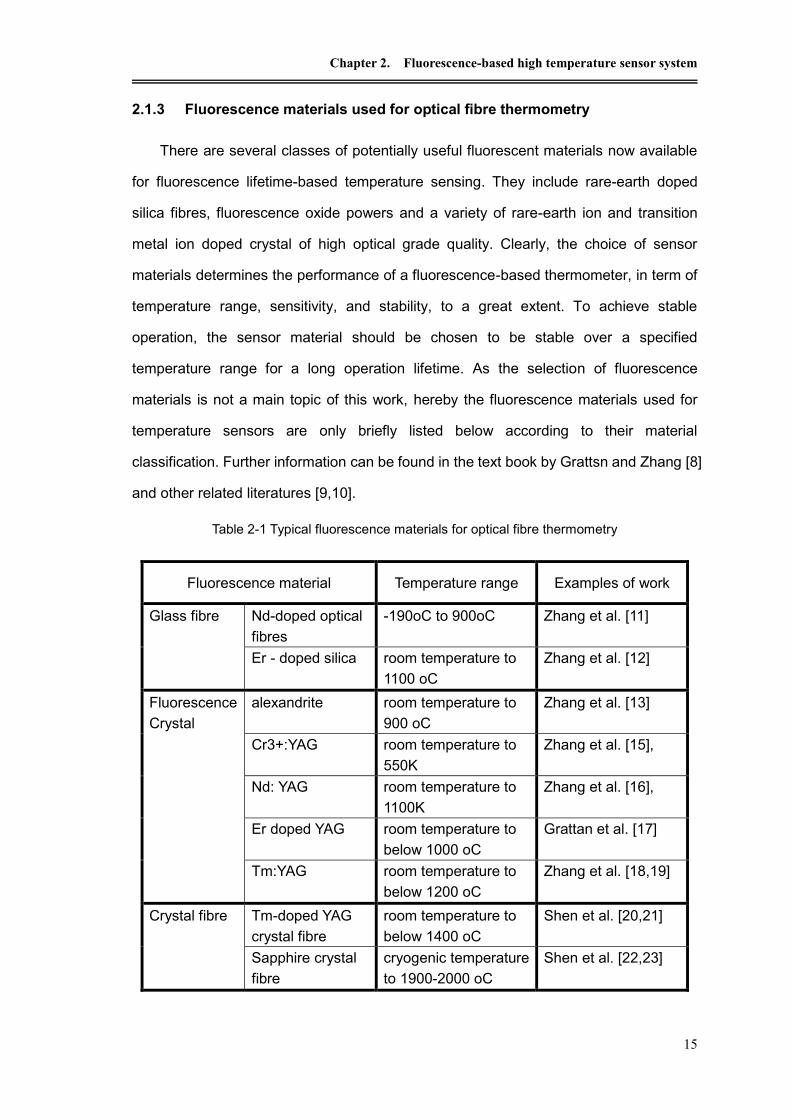
Chapter 2. Fluorescence-based high temperature sensor system
15
2.1.3 Fluorescence materials used for optical fibre thermometry
There are several classes of potentially useful fluorescent materials now available
for fluorescence lifetime-based temperature sensing. They include rare-earth doped
silica fibres, fluorescence oxide powers and a variety of rare-earth ion and transition
metal ion doped crystal of high optical grade quality. Clearly, the choice of sensor
materials determines the performance of a fluorescence-based thermometer, in term of
temperature range, sensitivity, and stability, to a great extent. To achieve stable
operation, the sensor material should be chosen to be stable over a specified
temperature range for a long operation lifetime. As the selection of fluorescence
materials is not a main topic of this work, hereby the fluorescence materials used for
temperature sensors are only briefly listed below according to their material
classification. Further information can be found in the text book by Grattsn and Zhang [8]
and other related literatures [9,10].
Table 2-1 Typical fluorescence materials for optical fibre thermometry
Fluorescence material Temperature range Examples of work
Glass fibre Nd-doped optical
fibres
-190oC to 900oC Zhang et al. [11]
Er - doped silica room temperature to
1100 oC
Zhang et al. [12]
Fluorescence
Crystal
alexandrite room temperature to
900 oC
Zhang et al. [13]
Cr3+:YAG room temperature to
550K
Zhang et al. [15],
Nd: YAG room temperature to
1100K
Zhang et al. [16],
Er doped YAG room temperature to
below 1000 oC
Grattan et al. [17]
Tm:YAG room temperature to
below 1200 oC
Zhang et al. [18,19]
Crystal fibre Tm-doped YAG
crystal fibre
room temperature to
below 1400 oC
Shen et al. [20,21]
Sapphire crystal
fibre
cryogenic temperature
to 1900-2000 oC
Shen et al. [22,23]

Optical fibre high temperature sensors and their applications
16
2.1.3.1 Silica Glass fibres for fluorescence lifetime thermometry
Silica optical fibres are clearly constitute a significan material, which has been
widely used in optical communications and fibre-optic sensing systems, for example,
the specific silica fibres doped with rare-earth ions, have been used as the gain media,
in applications of erbium doped fibre amplifiers (EDFA) and fibre lasers. As a result, a
wide range of doped glass fibres has been developed over the past twenty years,
particularly for laser studies. Some of these doped fibres, particularly rare earth doped
fibres, have been used for fluorescence thermometers. Among them, Nd3+ doped and
Er3+ doped silica-based fibres the most commonly used.
Zhang et al. [11] reported on the Nd-doped optical fibres for temperature sensing.
The lifetime characteristics over the temperature range from -190oC to 900oC were
evaluated, and it was shown that the probe made from this Nd-doped silica fibre is
suitable for temperature measurement over the wide temperature range below 700oC.
Erbium (Er) doped silica is another widely used and familiar fibre material among
the doped fibres that are widely commercially available. The characteristics of such fibre
are very well known because of its wide applications as erbium doped fibre amplifier
(EDFA). The fluorescence characteristics of the Er-doped silica fibre at elevated
temperatures have been extensively studied, e.g. by Zhang et al. [12]. The thermal
characteristics of the fluorescence decay of Er-doped fibres of different active dopant
concentration under similar conditions were observed. The results of the tests on the
fluorescence characteristics of the erbium doped fibres shown above seemed to
indicate that the fibres are good candidates for thermometry within the temperature
region from room temperature to below 1000 oC.
2.1.3.2 Fluorescence crystals used for fluorescence lifetime thermometry
Unfortunately, due to the difficulties in preventing the fibre material from
crystallization at high temperatures, silica glass fibres are not suitable for long-term
operation under elevated temperatures. Under these circumstances, the fluorescence
ion doped crystals may be a better candidate in terms of the performance stability at

Chapter 2. Fluorescence-based high temperature sensor system
17
high temperatures. Probes fabricated from crystal materials are normally preferred for
long-term high temperature applications, as the crystal materials are physically and
chemically stable without any tendency to becoming opaque after long-term operation
at high temperatures as long as the melting point of these crystal are substantially
higher than the working temperature concerned, These crystals can be transition metal
ion (for example, Cr3+) doped crystals or rear earth ion (for example Tm3+, and Nd3+)
doped crystals.
Cr3+ ion activated materials have shown wide optical absorption spectra, and a
significant variety of the temperature dependence of fluorescence lifetime, which makes
these materials a suitable candidate for a wide range of temperature measurement. A
range of Cr3+ doped crystals have been investigated as sensor elements in fluorescence
lifetime-based fibre thermometers. These crystals include alexandrite [13], emerald [14],
Cr3+:YAG [15], for example.
In addition to transition-metal ion doped crystals, rare-earth ion doped oxides or
crystals are good sensing materials for fluorescence lifetime-based thermometry.
Several types of rare-earth doped oxides and crystal garnets have been investigated
intensively, e.g., Grattan at al investigated the fluorescence characteristics of Nd:YAG at
elevated temperature up to 1100K [16].
Along with Nd: YAG, Er doped YAG also shows a strong fluorescence even at
temperatures up to 1100K. In the work reported by Zhang et al [17], a monolithic
crystalline fibre optic temperature sensor, with a tip of Er3+ doped YAG, was used as the
sensing material. The fluorescence lifetime versus temperature was determined over
the temperature range from room temperature to 1100K.
Zhang et al [18,19], investigated another type of fluorescence crystal of YAG
crystal, Tm:YAG, as a temperature sensing material, after some early work on thermal
florescence characteristics of Tm:Y2O3 power [20]. The fluorescence characteristics of
Tm-doped fibre were investigated up to the temperature of 1200oC. The results had
proved that these materials with a dopant of Tm3+ are good candidates for high

Optical fibre high temperature sensors and their applications
18
temperature measurement.
2.1.3.3 Crystal fibre-based fluorescence thermometry
Known as functional fibres, optical crystal fibres offer a combination of material
properties and waveguide geometry unavailable in either glass optical fibres or bulk
crystals. Compared to silica glass fibres, they usually appear as single-crystal fibres
with relatively large diameters and short length, and in most cases without cladding.
Crystal optical fibres were first introduced as a promising fluorescent sensing
candidate by Shen et al in 1996 [21]. The construction of the crystalline fibre probe, with
a certain length of sapphire (less than a millimetre) as temperature-sensing element on
the tip of a YAG crystal fibre, offers great advantage in performance. Firstly, the
thermometer probe is compact. Secondly, the probe can be used in severe conditions
where a normal fibre bundle cannot sustain or survive, as the YAG fibre is used as part
of the guiding fibre. Such a crystal fibre based thermometer can be operated in the
temperature range from cryogenic to very high temperature near the melting point of the
crystal fibre (1900-2000 oC) [22,23].
Among the fluorescence materials listed above and many other materials, Tm:YAG
crystal was selected in particular in this work as a sensing medium for a high
temperature sensor system due to its long fluorescence lifetime and stability at elevated
temperatures, while Nd doped fibre was used for a fluorescence-based fire alarm
system, which will be discussed in Chapter 3.
2.2 Fluorescence decay lifetime measurement schemes
In addition to the selection of appropriate fluorescence materials to meet the
requirements of the applications, the design of an effective, simple and economic
electronic system for the detection of the fluorescence decay lifetime is also a vital issue
in the development of a practical temperature sensor system with potential for
commercialization. Several signal processing techniques for the measurement of
fluorescence lifetime have been used and reported in fluorescence lifetime-based
temperature sensor systems and these can be categorized into three main approaches

Chapter 2. Fluorescence-based high temperature sensor system
19
according to the signal processing techniques used. The outlines of some of these
typical schemes are discussed in the following sub-sections.
2.2.1 Pulse measurement of fluorescence lifetime
In this approach, the excitation light applied to the fluorescence material is in the
form of a delta function or a rectangular pulse, and the measurement is carried out from
the observation of the fluorescence decay following the removal of the excitation light.
The following are some methods used to derive the lifetime from the decay signal which
have been used in some fluorescence lifetime-based thermometer systems
2.2.1.1 Two-point constant measurement method
This is a relatively straightforward method used by several research groups at the
early stage of the development of fluorescence-based sensor systems [7,24-25]. The
simple principle of this method is illustrated in Figure 2.2. The approach is to compare
the fluorescence intensity at two points along the exponential decay curve after the
termination of the excitation light. The electronics deployed for this measurement detect
the first value, Io of the decay signal at a fixed time, t1, after the removal of the excitation
light. When the decaying signal falls to the second intensity level, of the value Io/e, at the
time t2, when a “crossover” occurs is noted. The interval of between t2 and t1 is the time
constant, , of the exponentially decaying signal, and the time constant, , may be used
as the value of the fluorescence lifetime.
This type of approach is simple and inexpensive in relation to the electronic
components used. However, a significant disadvantage of this technique is that the
signal is only measured at two specific points, and as a result, the accuracy of it is
greatly limited.

Optical fibre high temperature sensors and their applications
20
Inte
nsi
tyIo
1
0
tt
eII
Exciting
light pulse
Time
Io/e
12 tt0t 1t
Figure 2.2 Principle of the two-point time constant measurement approach
2.2.1.2 Integration method
To achieve a higher accuracy from the pulse measurement approach, several
techniques have been developed which are based on the integration of the decaying
signal over different periods of time.
One example of this is the signal processing scheme introduced by Sholes and
Small [5]. As shown in Figure 2.3, when the decaying signal falls below a pre-set level,
the start measurement is triggered. The signal integration is performed over two fixed
time intervals, t1 and t2, and the integration values, A and B of this two periods are
sampled. When the time derivative of the signal has reached zero, the integrator is reset
and restarted, and the integrated noise and dc offset levels are then captured, and given
by the values of C and D, which are equivalent to the noise and dc offset components in
A and B respectively. Therefore, the fluorescence lifetime, , can be derived from the
following relation [5]:
/
/
2
1
1
1t
t
e
e
DB
CA
(2.1)

Chapter 2. Fluorescence-based high temperature sensor system
21
t1
t2 t2
t1
A
B
C
D
Inte
nsi
ty
Time
Integration
DC Offset
&Noise
Figure 2.3 Schematic illustration of Integration method
2.2.1.3 Digital curve fit method
Since high speed digital signal processors (DSPs) or data acquisition (DAQ) cards
are commercially available at relatively low cost, some fluorescence thermometry
systems utilizing digital data acquisition and signal processing have been developed
[26]. This kind of digital regression approach is termed as “digital curve fit method”,
which was described in detail by Sun [27].
In such a system, the fluorescence material is excited by sequential light pulses,
modulated by a TTL rectangular waveform, and as a result a periodic fluorescence
decay signal can be captured and processed. In doing so, a selected portion of the
decaying curve is digitally sampled. The digitalized samples, after a correction of any dc
offset, shown in Figure 2.4, are processed by the DSP or a PC to provide the best fitted
exponential curve, using a numerical algorithm, such as the least-squares curve fit and
single Prony method. Then the lifetime, , can be derived from the exponential curve.

Optical fibre high temperature sensors and their applications
22
An investigation into the errors caused by the dc baseline offset and noise in the
least-squares estimation of the exponential lifetime has been carried out by Dowell and
Gillies [28], It showed that such two-parameter estimation approach only estimates Io
and , and assumes zero baseline offset, therefore is rather sensitive to the small,
residual baseline offset. Thus a three parameter estimation, which includes the
estimation of the baseline offset, was proposed as a better solution. However, this
results in increasing the complexity of programme and prolonging the signal processing
time, though this is not a significant issue as the processing speed of PC is increasing
continuously every year.
2.2.2 Phase and modulation measurement
The technique of phase and modulation measurement of fluorescence lifetime is
schematically illustrated in Figure 2.5. The intensity of the excitation is sinusoidally
modulated, so that the fluorescence signal from the sensor material follows the same
sinusoidal pattern, but has a phase shift of behind the excitation light. The phase,
can be expressed as [29]:
f2tan (2.2)
Time
ln(I
)
Digitized smaples(After offset Correction)
Best linearcurve fit
ln(I)=-(1/)t+ln(Io)
Noisefloor
Figure 2.4 Illustration of digital curve fit technique

Chapter 2. Fluorescence-based high temperature sensor system
23
2f
m
2f
f
Inte
nsi
ty
Excitation Light
Fluorescence Response
0
0
where tan=2f and =phase difference
Figure 2.5 Phase and modulation measurement of fluorescence lifetime
Thus, the lifetime, , can be derived from the measurement of the phase shift, .
As inherently insensitive to dc offset and the ac noise in the sinusoidal signal, this
approach is of high accuracy and is mainly meant to be used in precision
instrumentation. Grattan et al. [29] have demonstrated the use of this technique in a
ruby fluorescence-decay thermometer, where a high-power green LED was used as the
excitation light source. Over the range from room temperature to 170 °C, a quite
satisfactory measurement deviation was achieved under a poor signal-to-noise ratio
condition. A similar system, reported by Augousti, et al., used alexandrite as the sensor
material and was capable of measuring temperature over a range 20 - 150 °C with an
accuracy of ±1°C and a response time of 1 sec [30].
However, since the system requires the measurement of fluorescence during the
excitation period, it is highly sensitive to the excitation light leakage to the detector and
the optics required to prevent such leakage can make the system very costly
2.2.3 Phase locked detection (PLD) scheme
This phase-locked detection of fluorescence lifetime is a signal processing
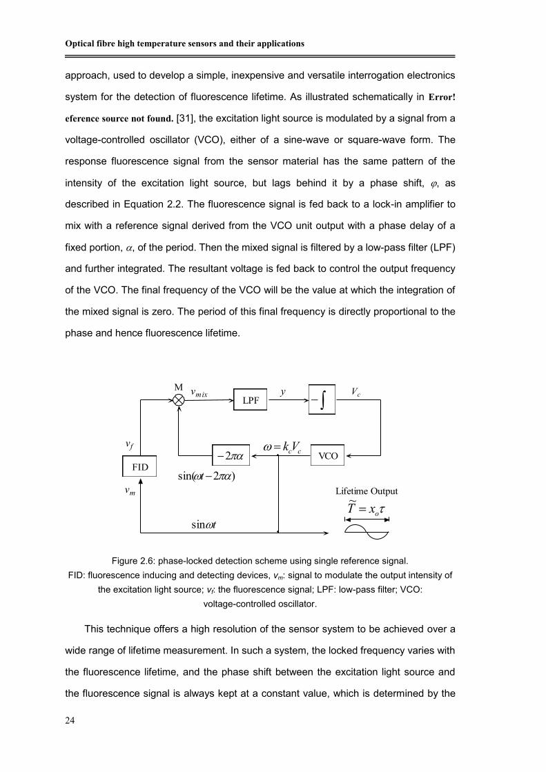
Optical fibre high temperature sensors and their applications
24
approach, used to develop a simple, inexpensive and versatile interrogation electronics
system for the detection of fluorescence lifetime. As illustrated schematically in Error!
eference source not found. [31], the excitation light source is modulated by a signal from a
voltage-controlled oscillator (VCO), either of a sine-wave or square-wave form. The
response fluorescence signal from the sensor material has the same pattern of the
intensity of the excitation light source, but lags behind it by a phase shift, , as
described in Equation 2.2. The fluorescence signal is fed back to a lock-in amplifier to
mix with a reference signal derived from the VCO unit output with a phase delay of a
fixed portion, , of the period. Then the mixed signal is filtered by a low-pass filter (LPF)
and further integrated. The resultant voltage is fed back to control the output frequency
of the VCO. The final frequency of the VCO will be the value at which the integration of
the mixed signal is zero. The period of this final frequency is directly proportional to the
phase and hence fluorescence lifetime.
This technique offers a high resolution of the sensor system to be achieved over a
wide range of lifetime measurement. In such a system, the locked frequency varies with
the fluorescence lifetime, and the phase shift between the excitation light source and
the fluorescence signal is always kept at a constant value, which is determined by the
LPF
VCO
FID
oxT ~
Lifetime Output
M yvmix
vf
vm
Vc
2
tsin
)2sin( t
ccVk
Figure 2.6: phase-locked detection scheme using single reference signal.
FID: fluorescence inducing and detecting devices, vm: signal to modulate the output intensity of
the excitation light source; vf: the fluorescence signal; LPF: low-pass filter; VCO:
voltage-controlled oscillator.

Chapter 2. Fluorescence-based high temperature sensor system
25
reference signal delay ratio, . Therefore this category of techniques has been termed
the "phase-locked detection" by Zhang et al [31].
2.2.3.1 Simple Oscillator Method
Bosselmann reported the earliest scheme which is closely related to the
phase-locked detection technique [32]. In this scheme, a positive feedback is formed by
sending the fluorescence response signal back to control the output intensity of the
excitation light source, via a timing circuit which amplifies the signal with an added
phase shift, so that the system will oscillate at a frequency determined by the
combination of the time-constant of the timing circuit and the fluorescence lifetime. The
measurement of the lifetime is then derived from the oscillating frequency, which is
subject to the parameter drifts of the timing circuit. The sensitivity of the frequency to the
lifetime is also limited by the fact that is given by the combination of the lifetime and the
time-constant of the timing circuit.
2.2.3.2 Phase-locked detection using single reference signal
A primitive form of the phase-locked detection scheme was reported by
Bosselmann et al [6], as a revision of the simple oscillator method, and it was termed as
phase-locked detection using single reference signal later by Zhang et al [31] .The
operational principle of the scheme is similar to that illustrated in Figure 2.6, except that
a square-wave type of VCO unit is used, thus excitation light is square-wave modulated.
Bosselmann pointed out that the measurement sensitivity of using square-wave
modulation had been enhanced by a factor of 2 than that of using sinusoidal modulation,
after a comparison was made between this primitive phase-locked detection scheme
and the simple oscillator scheme mentioned above. This difference arises from the
electrical system configurations rather than the modulation schemes used. In the simple
oscillator system, the fluorescent material is directly used as a timing component in the
oscillator by means of optoelectronic coupling. The oscillating frequency is determined
by the combination of the fluorescence lifetime and the time-constant of an additional
electronic timing circuit, which limits the sensitivity of the oscillating frequency to the

Optical fibre high temperature sensors and their applications
26
lifetime. However, in the phase-locked detection system, the oscillation is generated by
a VCO with the oscillating frequency only controlled by the fluorescence lifetime, and
thereby the sensitivity of the frequency to the lifetime is higher than that in the former
case.
Several groups have demonstrated the success of utilizing this scheme [6,33-34]
for fluorescence thermometers, confirming that this interrogation scheme is highly
suited to high precision, wide range applications. However, as the system requires the
measurement of fluorescence during the excitation period, even a tiny fraction of
excitation light leaking into the photodetector will seriously degrade the performance of
the system. An excess of such leakage can even cause the system to fail [31].
Therefore, high quality filter optics are needed to prevent such leakage and this could
make the system costly and bulky.
2.2.3.3 Phase-locked detection using two reference signals
This version of phase-locked detection has been introduced by Zhang et al [35] to
overcome the problem of excitation light leakage in a high-temperature measurement
fluorescence based system using phase-locked detection with one reference. In this
approach, two reference signals derived from the VCO output are used to mix
successively with the fluorescence signal to delete the excitation leakage component
from the signal. The integration of the mixed signal is then used to control the oscillating
frequency of the VCO.
This technique, which has been proved both theoretically and experimentally, is
intrinsically immune to the impact of the excitation leakage. Therefore, it is no longer
necessary to use expensive and complex optical arrangements.
In this work, a fluorescence lifetime-based thermometry system is developed based
on the phase-locked detection using two reference signals approach and the details of
which will be discussed in Section 2.3. The details about the fluorescence lifetime
measurement schemes and the techniques used are summarized by Zhang et al [8,9].

Chapter 2. Fluorescence-based high temperature sensor system
27
2.3 Design of the fluorescence-based temperature sensor system
A robust fluorescence lifetime based temperature sensor system has been
successfully developed and evaluated in this work, based upon the phase-locked
detection scheme with two reference signals as discussed above in section 2.2.3.3, and
the use of Tm:YAG as sensing element, to address the challenges arising from a range
of temperature measurements needs. The details of the sensor system design are
discussed in this section.
2.3.1 Sensor probe configuration
A typical configuration of Tm:YAG crystal fluorescence temperature probe, for low
temperature applications, is shown in Error! Reference source not found.. A piece of
m:YAG crystal polished to a small rod with a diameter of around 330m is used as
sensing tip. Subsequently the Tm:YAG rod and a 300/330 m silica fibre are inserted
into a 570/700 m silica glass capillary. Both are fixed in the capillary using epoxy resin
at the tips for good optical coupling, which is vital for obtaining strong fluorescence
signal from the sensing material. Then the capillary with the fibre and the Tm:YAG rod is
inserted into a stainless steel tubing for protection. If the probe is used to measure
temperature in some environment, such as in microwave environment, where steel itself
is heated by the microwave energy, a ceramic tubing may be used to replace the
stainless steel tubing. As epoxy resin, which cannot sustain temperatures higher than
300oC~400oC (even with special high temperature epoxy), is used, this type of probes
can only be used for some low temperature measurement applications (less than
400oC).
For the high temperature (over 400oC) applications, there is no high temperature
sustainable epoxy commercially available. In addition, the sensing materials may also
react with the epoxy at high temperatures, which can degrade the fluorescence signal,
and hence degrade the temperature measurement ability of the system. In order to
achieve good optical coupling under elevated temperatures, a special approach has to

Optical fibre high temperature sensors and their applications
28
be used for assembling the probe. Instead of using epoxy resin to fix the Tm:YAG rod
and the fibre, as for the low temperature probes, fusing and shrinking of the silica
capillary can be used to fix the core components. After the crystal rod and the fibre
being inserted into the capillary, the capillary is fused using a high temperature
miniature torch at several points along the fibre, one of which is used to fix the Tm:YAG
rod with the capillary. While the capillary is cooling down immediately after the torch
having been removed, it shrinks to fix the position of the Tm:YAG rod and the fibre
within the capillary. Careful handling is required to avoid breaking the delicate capillary
and melting the silica fibre and this can be achieved by carefully controlling the flame of
the torch and the distance between the torch and the capillary. The configuration of this
type of probes is illustrated in Figure 2.8Error! Reference source not found.. As there is
no epoxy involved at the tip of senor material, the probe can be used for high
temperature measurements and the sensing range is only limited by the measurement
range of fluorescence lifetime, which can be up to 1000oC, or higher than 1100oC if
Tm:YAG Crystal
Epoxy Resin
Steel tubingSilica glass capillary
300/330m Silica fiber
100~400mm ProbeSilica glass fibre
SMA Connector
Protection tubing
Figure 2.7 Configuration of Tm:YAG probe for low temperature applications
Tm:YAG Crystal
Epoxy Resin
Steel tubing Silica glass capillary
300/330m Silica fiber
Protection tubing
fusion points
Figure 2.8: Configuration of Tm:YAG probe for high temperature applications

Chapter 2. Fluorescence-based high temperature sensor system
29
radiation compensation is introduced [36].
2.3.2 Interrogation system design and the PLD approach
An enhanced model of a sensor interrogation system was built in this work on the
basis of phase-locked fluorescence detection using two reference signals, which was
first introduced by Zhang et al [35]. The sensor system, connected to a PC via a
user-friendly interface as shown in Figure 2.9, is illustrated in Figure 2.10. A 785 nm
Laser, modulated by the TTL signal from the PLD unit, is used as the pump light source,
and its light is launched to the sensor probe through a Y-coupler to excite the Tm:YAG
crystal. The fluorescence signal generated is collected and coupled back to a PIN
photo-detector. This signal is processed by the PLD unit to lock the modulation
frequency in respect to the fluorescence signal. The modulation frequency is then
measured by a microchip unit, which performs the frequency measurement, and passed
to a PC for lifetime calculation. Thus its corresponding temperature value can be
obtained based on the calibration data obtained prior to the tests.
Figure 2.9: Fluorescence lifetime-based thermometer connected with a PC
PC with Interface
Interrogation Box
Probe

Optical fibre high temperature sensors and their applications
30
Figure 2.10: System setup of enhanced fluorescence lifetime-based thermometer
As shown in Figure 2.10, an AT80C51 microprocessor was specifically designed to
be included in the signal processing system to detect the laser modulation frequency (or
period), which is proportional to the fluorescence lifetime of the fluorescence-based
temperature sensor probe. The microprocessor unit is connected to the PC via a
RS-232 serial port for data transmission. As a result there is no need for a timer card
and any standard computer, including laptop, can be readily used for the temperature
measurement. This makes experiments carried out outside the laboratory much easier
to perform as a dedicated computer with timer card added-on is not needed.
Due to the multi-functionality of the mono-chip microprocessor used, the developed
fibre thermometer system has the potential for a multi-channel temperature
measurement, for example, for the measurement of heat flux which requires
simultaneous multi-point temperature measurements.
2.3.2.1 Design of the phase locked detection system for fluorescence lifetime
measurement
The pulse modulated phase locked detection (PLD) with two references
(PLD-PMTR) method used for this system is illustrated schematically in Figure 2.11[35].
This approach is created to eliminate the excitation leakage, which is caused by the
excess radiation from the light source reaching photo-detector along with the
fluorescence signal. The waveforms of the signals designed are illustrated in Figure
2.12.
LD Driver
Photo-detector
PLDModule
Mono-chipMicroprocessor
PC
RS232
To Probe
100/140m
300m
TTL outputOptical fiber
bundle300/340m
Fluorescence

Chapter 2. Fluorescence-based high temperature sensor system
31
LPF
VCO
Delay
)2/~
(T
FID
21
oxT ~
Lifetime Output
M1 M2yvmix1 vmix2
vf+l
vmmv
Vc
.
.
.
vr2vr1
Figure 2.11: phase-locked detection of fluorescence lifetime using two reference signals
(components as Figure 2.6)
With the presence of the excitation leakage, the output from the fluorescence
inducing and detecting device (FID) is given by [35]
)()( tvtvv lflf (2.3)
where vf(t) is the actual fluorescence response, and vl(t) is the excitation leakage.
Therefore the output of mixer M1 and M2 in Figure 2.11, vmix1 and vmix2, could also be
expressed as the sum of their fluorescence and excitation leakage components
respectively, as depicted in Figure 2.12, where the upper traces show the components
corresponding to the fluorescence signal, and the lower traces corresponding to the
excitation leakage. As the leakage signal is in the phase of the modulation signal mv
and is rectangularly profiled, thus lfv is given by[35]:
TtTVtv
TtVtvtvtvv
lof
lof
lflf ~2/
~,)(
2/~
0,)()()( (2.4)
where Vlo is the amplitude of the excitation leakage
As illustrated in Figure 2.12, the output of the first mixer, M1, is given as follows[35]:
2/~
0,)(1 TtVtvv lofmix (2.5)
and

Optical fibre high temperature sensors and their applications
32
Figure 2.12: Output waveforms of PLD

Chapter 2. Fluorescence-based high temperature sensor system
33
)()2/~
( 11 tvTtv mixmix (2.6)
Thus the output of phase sensitive detector (PSD), y, is given as[35]:
2
~
2
~)2/1(
2
~)2/1(
2
~
2
~
2
~
2
~)2/1(
2
~)2/1(
2
~
2
~
2
~
)()()(~2
)()()(~2
)(~2
)(~1
0
0
02
~
02
T
T
T
T
T
T
T
T
T
T
T
dttvdttvdttvT
dttvdttvdttvT
dttvT
dttvT
y
lololo
fff
mix
T
mix
(2.7)
where the last part of the above equation is zero. y is determined only by the actual true
fluorescence response as depicted in Figure 2.12. It can be shown that [35]:
)1(
)21)(1(4),(
2/
)4/2/4/
x
xxx
lo
ex
eeekVxfy
(2.8)
where k is the gain of the phase delay unit, is the phase delay, and x is the ratio of the
period of the modulation signal T~
, to the lifetime, , given by Equation 2.9 [35].
/~Tx (2.9)
The integrated value y is independent to the excitation leakage. Thus the system is
theoretically immune to the effect of excitation leakage.
When y=0, it is a “locked” state for the phase-locked detection system, which
means keeping the modulation period to the lifetime ratio at the value given by [35]:
0),(| xfo xx (2.10)
Thereby, the measurement of the fluorescence lifetime can be made from the
measurement of the modulation frequency using the following formula [35]:
oxT ~
(2.11)
2.3.2.2 Electronic design of fluorescence sensor interrogation system
A modular configuration of the hardware design was introduced to ensure the

Optical fibre high temperature sensors and their applications
34
robustness of the sensor system. The electronic system of the fluorescence
lifetime-based temperature sensor system can be divided into three main modules:
PLD module: Florescence lifetime measurement (to a period proportional to
lifetime)
Photo detector module: Weak fluorescence signal detection and
amplification
Micro-processor module: period measurement and data transfer.
Each module is laid on one standard DIN card and linked with other cards via the
interface board. This configuration makes the system much more flexible and easy to be
debugged, as the modular cards are interchangeable. Figure 2.13 shows the sensor
interrogation system with three modular DIN cards inside. The design of the electronic
circuits of these modules is discussed below.
Figure 2.13: Fluorescence lifetime-based temperature sensor interrogation system
PLD module
The operational principle of the PLD has been discussed in the previous sections.
Laser @985nm
Microchip Module
PLD Module
Photo Detector Module

Chapter 2. Fluorescence-based high temperature sensor system
35
The electronic system to perform this PLD function is illustrated in Figure 2.14. The
corresponding output and waveform are shown in Figures 2.11 and 2.12 respectively, as
described previously.
Figure 2.14: Electronic circuit of PLD module
Photo detector module
An extended InGaSn PIN photo detector was used to convert the optical
VCO
Logic circuit
(Delay, ÷2 and -1)
M1 (mix1)
M2 (mix2) -∫

Optical fibre high temperature sensors and their applications
36
fluorescence signal from the excited sensor material into a voltage signal. A I-V
converter and a two-stage amplifier, as illustrated in Figure 2.15, were used to amplify
the weak fluorescence signal to enable it to be processed by the PLD module.
Micro-chip processor module
The main electronic circuit of the micro-chip processor module is shown in Figure
2.16. This is used to perform the period measurement and send the measurement data
to a connected PC via RS232 serial port. The details of the design will be discussed in
the following sections.
Figure 2.16: Circuit of micro-chip processor for period measurement
Figure 2.15: Photo detector module of the fluorescence lifetime-based thermometer
FID

Chapter 2. Fluorescence-based high temperature sensor system
37
2.3.2.3 Microchip system for the optical thermometer
Measurement of the modulation period
The modulation period, T~
, proportional to the fluorescence lifetime, , normally is a
rectangular TTL signal, and it can be measured using a timer card, as used by Zhang
et al [35]. In such an approach, a dedicated PC with a timer card added-on has to be
used, which hinders field applications of the system. Therefore, another method using
AT89C51 microchip to measure the modulation period,T~
, was developed in this work.
The schematic of the system is illustrated in Figure 2.17. In the system, the
modulation TTL signal from the PLD module is connected to the timer/counter, T1, of the
AT89C51. The internal pulse number, np, is counted between two consequent rising
edges of the TTL signal using the T1 counting function. Then the period of the signal,T~
,
can be derived using the given formula as:
pp TnT ~
(2.12)
where Tp is the internal pulse period, which is related to the oscillator frequency of the
microchip system.
AT89C51MAX232
PC
TXD 11
RXD 10
10
9 8
7
PLD
ModuleRXD
TXD13 INT0
T~
Modulation
TTL signal
Period measurement Data communication via RS232
Figure 2.17: Schematic setup of the AT89C51 module for period measurement
AT89C51 microchip has two timers/counters, T0 and T1, and they can all work at
four different modes.
1) Mode 0
In mode 0, the timers are an 8-bit counter with a divide-by-32 prescaler, and the

Optical fibre high temperature sensors and their applications
38
timer registers (TL, TH) are configured as 13-bit registers.
2) Mode 1
Mode 1 is as same as mode 0, except the registers are configured as 16- bit ones
3) Mode 2
Mode 2 configures the timer register as an 8-bit Counter (TL1) with automatic
reload.
4) Mode 3
Timer 1 in Mode 3 simply holds its count. The effect is the same as setting TR1 = 0.
Timer 0 in Mode 3 establishes TL0 and TH0 as two separate counters.
In the fluorescence-based system, mode 1 of timer/counter T1 is used for
measurement of the period of the modulation signal. The flow chart, depicted in Figure
2.18, shows the procedure of the period measurement using mode 1 of timer T1. As a
16 bit counter it is not enough to hold the pulse counts of the period, another 8 bit
ResetTH1, TL1, TR1Start counting
Counter numberadd 1
counterover flow
ADD TO1, 1
Secondrising edge?
Next count
N
N
T1 stops countingOutput
TH1,TL1,TO1
Y
INT1 triggedT1 starts counting
First TTL signalRising edge
INT0Interupt End
Figure 2.18: Flow chart of period measurement using timer/counter of AT89C51

Chapter 2. Fluorescence-based high temperature sensor system
39
register, TO1, was assigned to hold the overflow of the counter registers (TL1 and TH1).
Hence the pulse count number is given by:
1
3
1
2
1 256256256 TOTHTLnp (2.13)
Data communication between PC and the sensor interrogation system
The data communication of the sensor interrogation system is linked to the PC via
the RS-232 serial port. The hardware connection is illustrated in Figure 2.16, with the
protocol being described in Figure 2.19, showing how the connection and the
communications between the PC and the interrogation system are established.
"E" received?
Send data"E", TH1. TL1, TO1
to COM
End
Y
INT0 triggedSend "E" to COMPC data reteive
requistSerial port interupt
Hand shakingsignal checking
Send data to COM
Read COM
Waiting for data
PC Thermometer
Calculate period
"E" is the preset hand shaking
N
Figure 2.19: data communication between fluorescence thermometer and PC
2.3.3 Interface software
A user-friendly interface, written in Delphi language, has been developed for the
fibre thermometer. The main functions of the interface software include the remote
control of the microprocessor, thus the sensor system, from the host PC, data retrieve,

Optical fibre high temperature sensors and their applications
40
data processing and display of experimental results, etc.
The function of remote control and data transmission between the microprocessor
of the sensor unit and the computer are realized via a RS232 serial port. The computer
sets the sample request rate of the fluorescence lifetime and data transmission is made
upon request from the computer. The fluorescence lifetime data received from the
sensor unit are then processed and converted to the measured temperature value
based on the stored calibration data.
The measurement results of fluorescence lifetime thus temperature variation
(a)
(b)
Figure 2.20: Screen print out of the fluorescence thermometer
(a) Graphic (b) Data sheet presentation of results
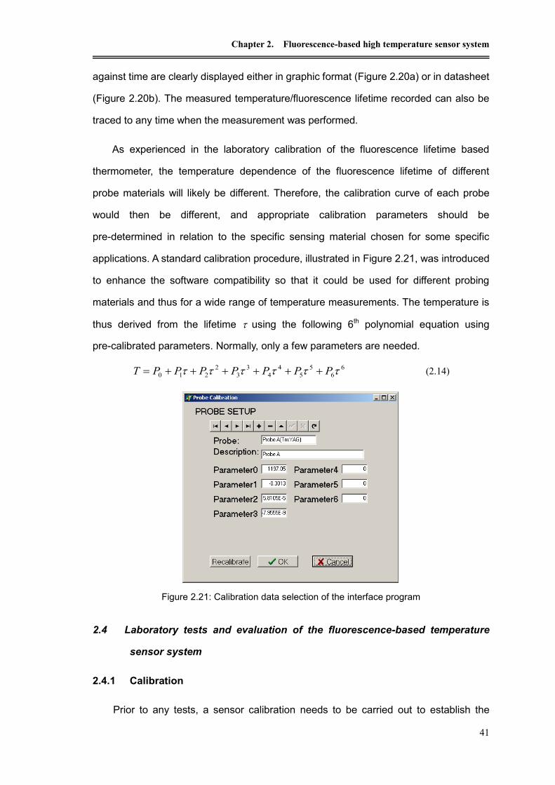
Chapter 2. Fluorescence-based high temperature sensor system
41
against time are clearly displayed either in graphic format (Figure 2.20a) or in datasheet
(Figure 2.20b). The measured temperature/fluorescence lifetime recorded can also be
traced to any time when the measurement was performed.
As experienced in the laboratory calibration of the fluorescence lifetime based
thermometer, the temperature dependence of the fluorescence lifetime of different
probe materials will likely be different. Therefore, the calibration curve of each probe
would then be different, and appropriate calibration parameters should be
pre-determined in relation to the specific sensing material chosen for some specific
applications. A standard calibration procedure, illustrated in Figure 2.21, was introduced
to enhance the software compatibility so that it could be used for different probing
materials and thus for a wide range of temperature measurements. The temperature is
thus derived from the lifetime using the following 6th polynomial equation using
pre-calibrated parameters. Normally, only a few parameters are needed.
6
6
5
5
4
4
3
3
2
210 PPPPPPPT (2.14)
Figure 2.21: Calibration data selection of the interface program
2.4 Laboratory tests and evaluation of the fluorescence-based temperature
sensor system
2.4.1 Calibration
Prior to any tests, a sensor calibration needs to be carried out to establish the

Optical fibre high temperature sensors and their applications
42
relationship between the fluorescence decay lifetime and the measured temperature.
Before the calibration, the sensor probes are required to be annealed at a temperature
higher than the maximum temperature to be measured to enable the stability and
repeatability of the sensor. In this specific work the probe was annealed at 800oC for 48
hours before the calibration. The typical procedure of calibration and results obtained
are presented below.
The fluorescent lifetime was monitored using the PLD fluorescence lifetime
measurement system developed above. No observable lifetime change was observed
during the annealing process when the probe was placed at 800oC. Subsequently
when the annealing temperature was raised to 900 oC, a significant lifetime change was
observed within one hour. The annealing process at 900 oC was then stopped after one
hour, but restarted as temperature dropped to 800oC again. No lifetime change was
observed again as expected under the temperature of 800 oC.
Following the annealing, the probe was then calibrated using the readout system
developed along with a K-type thermometer. The calibration curve of the fluorescence
lifetime against temperature is presented in Figure 2.22., The calibration curves of
different probes have a slight difference from each other, due to the different annealing
process and small the material differences. However, each single probe does
demonstrate a high repeatability (deviation less than 0.1%) when experiencing cycles of
temperature going up and down (ranging from room temperature to 750 oC) after
annealing.

Chapter 2. Fluorescence-based high temperature sensor system
43
2.4.2 System performance
2.4.2.1 Temperature measurement – cross comparison with K-type
thermocouple at laboratory
A cross-comparison between the fibre thermometer developed and a K-type
thermocouple was made when both probes were placed intimately at the same centre
position of a Carbolite tube oven, which can reach a maximum temperature of 1200oC.
Considering different dynamic responses of the probes, measurements were taken at
each temperature after 30 minutes with an increment of 50 0C from the room
temperature to nearly 800oC. Then the power supply of the oven was shut off, and the
temperature fell naturally to the room temperature. In Figure 2.23, the readings of the
thermocouple thermometer and the optical fibre thermometer are shown. A good
agreement between the fibre fluorescence thermometer and the thermocouple could be
found, the differences between them was less than ±1oC, as shown in Figure 2.24.
Further tests have shown that with this fluorescence lifetime measurement system,
using the above calibration data, a temperature resolution of 1 oC was realized over the
Temperature (oC)
0 200 400 600 800
Life
tim
e (
us)
1000
2000
3000
4000
5000
6000
7000
8000
9000
Calibration 1
Calibration 2
Figure 2.22: Lifetime versus temperature characteristics of Tm:YAG
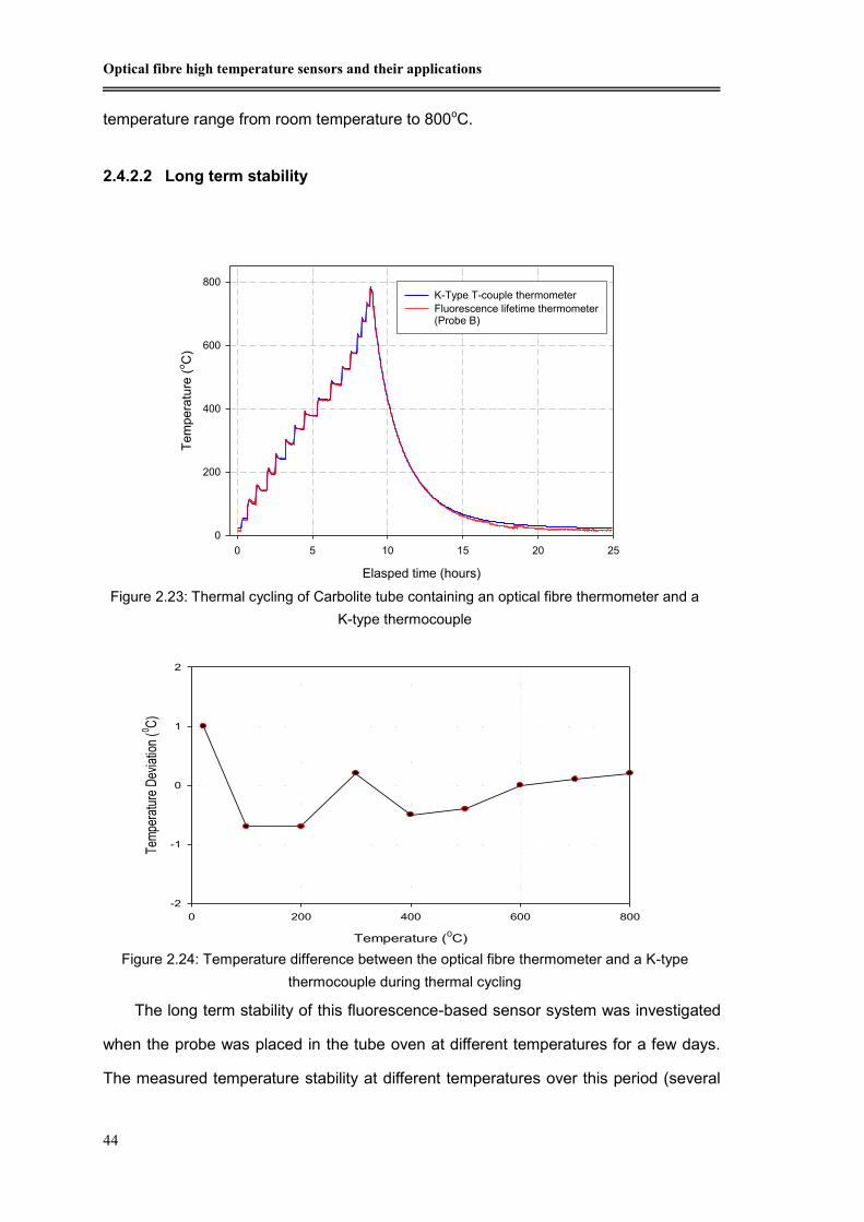
Optical fibre high temperature sensors and their applications
44
temperature range from room temperature to 800oC.
2.4.2.2 Long term stability
The long term stability of this fluorescence-based sensor system was investigated
when the probe was placed in the tube oven at different temperatures for a few days.
The measured temperature stability at different temperatures over this period (several
Elasped time (hours)
0 5 10 15 20 25
Tem
pe
ratu
re (
oC
)
0
200
400
600
800
K-Type T-couple thermometer
Fluorescence lifetime thermometer(Probe B)
Figure 2.23: Thermal cycling of Carbolite tube containing an optical fibre thermometer and a
K-type thermocouple
Temperature (0C)
0 200 400 600 800
Tem
pera
ture
Dev
iatio
n (0 C
)
-2
-1
0
1
2
Figure 2.24: Temperature difference between the optical fibre thermometer and a K-type
thermocouple during thermal cycling

Chapter 2. Fluorescence-based high temperature sensor system
45
hours at each temperature) is shown in Figure 2.25. A standard deviation of the
measurement ranging from 0.97 oC to 0.13 oC was estimated over the temperature
region from room temperature to nearly 800 oC and the results are shown in Figure
2.26.
Elasped Time (hours)
0 5 10 15 20 25 30 35
Tem
pera
ture
(0C
)
0
200
400
600
800
100 0C
200 0C
298 0C
397 0C
500 0C
601 0C
700 0C
792 0C
Figure 2.25: Long term stability of the fluorescence thermometer
Temperature (0C)
0 200 400 600 800
Sta
ndar
d D
evia
tion
(0 C)
0.0
0.2
0.4
0.6
0.8
1.0
1.2
1.4
Figure 2.26: Standard deviation of the fluorescence thermometer at different temperatures

Optical fibre high temperature sensors and their applications
46
2.4.3 Main specifications of the fluorescence thermometer
As a summary of the laboratory test, the main specifications of the fluorescence
decay lifetime thermometry system using the PLD approach are listed in table 2.1
Table 2-2 Main specifications of the fluorescence thermometer
Sensor Material Tm:YAG crystal
Operation temperature range Rroom temperature to 900oC
Temperature resolution 1oC
Maximum measurement error ±2oC
Stability (fluctuation)
±1oC (1 hour)
±2oC (5 hours)
±2.5oC (5 hours)
Response time ~1 second
2.5 Applications of the fluorescence-based temperature sensor
Along with the series tests and evaluation of the fluorescence lifetime-based
temperature sensor system developed in the laboratory environment, the system has
been used and tested in some industrial contexts with the help from industrial partners
for some industrial process controlling and monitoring applications, and some typical
applications are presented in the following sections.
2.5.1 High temperature measurement at Corus, UK
The fluorescence lifetime-based thermometer system, tested and evaluated at the
laboratory environment, clearly shows that the system can operate at temperatures up
to 900oC over a long period, and therefore shows potential for monitoring the refractory
furnace linings in the steel industry, where a real-time and reliable monitoring and
control of the temperature of furnaces is required.
An evaluation of this fibre thermometer in the practical industrial field was carried out
at Corus, Teeside Technology Centre, Middlesborough, UK. The performance of the
fibre thermometer was compared with that of a K-type thermocouple when they were

Chapter 2. Fluorescence-based high temperature sensor system
47
both inserted into the inside of a refractory brick, which was the same type used
currently in steel furnace as lining. The experimental setup of the test is shown in Figure
2.27.
The refractory brick, which was placed in an oven, was heated up gradually by the
high surrounding ambient temperature. The temperature inside the brick, where the
probes were located, would gradually rise until reaching the equilibrium state, if
sufficient time was given. After having reached the thermal equilibrium state, the power
of the oven was then switched off, and the surrounding ambient temperature of the oven
dropped quickly and the temperature inside the brick would fall following the ambient
temperature. As a refractory brick in the furnace was of high quality, both the process of
heat flowing in or out from the brick took a long time. For evaluating the dynamic
performance of the system, both the probes of the fibre thermometer and of the
thermo-couple were taken out from the brick and then put into the brick again quickly on
two separate occasions during the whole process. Two separate cycles of tests were
performed, and the results of the temperature measured from the fibre thermometer and
the thermo-couple against time are illustrated in Figure 2.28, showing a good
Figure 2.27: Experimental setup of the test carried out at Corus
Sensor Unit
PC with Interface
Probe

Optical fibre high temperature sensors and their applications
48
agreement between of the two independent temperature measurement devices in
responding to the temperature changes.
Figure 2.28: Test results of the fluorescence based thermometer and of the thermocouple at
Corus
2.5.2 Temperature monitoring of a precision free electron laser heating process
This is a novel application of the fibre fluorescence temperature sensor system in
the establishment and monitoring of stable temperature conditions for precision
adhesion of small components in the semiconductor industry. The specific application is
to heat and thus prepare a small globule of adhesive on the back of a precision
integrated circuit which is to be used to adhere it to a credit card - the process of the
manufacture of “smart cards” widely used by consumers. The temperature must be
carefully monitored and thus controlled to prevent damage to the delicate, thin chip and
to ensure the optimum conditions for adhesion to the credit card.
To achieve efficient, precision heating, a microwave free electron laser (FEL) is used
Cycle 1
Elapsed time (minutes)
0 50 100 150 200 250
0
200
400
600
800
Thermocouple Fibre thermometer
Cycle 2
Elapsed time (minutes)
0 20 40 60 80 100 120
0
100
200
300
400
500
600
700
Thermocouple Fibre thermometer
Tem
per
atu
re (
oC
) T
emper
ature
(oC
)

Chapter 2. Fluorescence-based high temperature sensor system
49
to deliver a precise amount of power onto the glue sample, taking full advantage of the
highly directional properties of the laser beam [37]., As shown by this work,
thermocouples and other electrically-based thermometer systems suffer from
self-heating due to “pick up” from the microwave fields and thus cannot be used for
precision temperature measurement. They always read “higher” than the actual
temperature under such circumstances in which microwave energy is present. Thus
optical technology, here the fluorescence lifetime-based thermometry, with the inherent
immunity to electromagnetic interference (EMI), offers a satisfactory alternative to the
electrical based thermometry. The benefits of the use of an accurate optical fibre
temperature sensor of this type are clearly demonstrated in this application, opening up
the possibility of the use of the same monitoring technique for other cases where
microwave radiation is used
Figure 2.29 shows a group of integrated circuits for smart cards with a small coin (a
one penny piece) for comparison of size. In order to fix these circuits to the plastic card,
a small globule of adhesive was applied on the back of a chip before it was heated by
the FEL microwave. The system setup for focused adhesive heating was shown in
Figure 2.30, where the power from the laser is delivered by the microwave waveguide
and two temperature probes, one an optical probe and the other a K-type thermocouple,
were mounted in such a way that they touched the surface of the glue. The temperature
change was monitored at the same spot on the surface.

Optical fibre high temperature sensors and their applications
50
Figure 2.29: Integrated circuits for smart cards
Figure 2.30: Setup for adhesive curing using Microwave FEL
Several samples were tested when the microwave FEL was switched on and off
over the period of the fast heating of the glue. A typical result of such a test is shown in
Figure 2.31, where the data from both thermometers are illustrated. The temperatures
read from both thermometers were consistent before the FEL was switched on, showing
Smart Chips
Smart Chips
Fibre probe
Microwave chamber

Chapter 2. Fluorescence-based high temperature sensor system
51
that both techniques used were applicable under normal conditions. However, once the
FEL was switched on, the adhesive was immediately subjected to the focused heating
of the microwave beam and the data obtained from the two sensors demonstrated a
dramatic difference due to the fact that the thermocouple itself was experiencing
‘self-heating’. As a result, it was no longer able to show the ‘true’ temperature of the glue
surface in this microwave environment. By contrast, the optical fibre sensor was
immune to the microwave interference and performed in a satisfactory way to give a
accuracy temperature measurement. After the FEL was switched off, the thermocouple
gradually cooled down and the temperature monitored was approximately the same as
to that read by the optical fibre sensor.
Figure 2.31: Adhesive temperature monitoring using the thermocouple and the optical fibre
sensor
In most practical cases of adhesive temperature monitoring, it is preferable that the
inner temperature rather than the surface temperature of the adhesive is to be
monitored. In such cases, care is needed to be taken to ensure that the probe could be
removed easily from the adhesive after the measurement is finished.
Polytetrafluoroethylene (PTFE) material proved to be satisfactory for protecting the
probe from the glue without degrading the sensor performance. The experimental
results under a similar procedure of switch on and off of the microwave FEL, obtained
Elapsed time (seconds)
400 500 600 700 800
20
30
40
50
60
70
Thermocouple Optical fibre sensor
Microwave
Off Off On
Tem
pera
ture
(oC
)

Optical fibre high temperature sensors and their applications
52
using a PTFE coating around the probe, are shown in Figure 2.32.
Figure 2.32: Adhesive temperature monitoring using the thermocouple and the optical fibre
sensor (wrapped with PTFE tape) during the on-off process of the microwave FEL
To verify that it was the thermocouple over-reading the temperature rather than the
fibre fluorescence base system under-reading the temperature, a test was carried out
for measuring the water heated with FEL. The output power was varied to change of the
water temperature. As shown in Figure 2.33, thermocouple read a temperature >100C
while the fluorescent thermometer shows a value below 100C, when the water was not
boiling. This result clearly indicates that the thermocouple was over-reading when the
FEL was on, and thus the optical fibre thermometer is a better suited candidate in such
environment where microwave energy is present.
Elapsed time (seconds)
0 100 200 300 400 500 600
0
50
100
150
200
250
Thermocouple Optical fibre temperature wrapped with PTFE tape
Microwave
Off On Off
Te
mp
era
ture
(oC
)

Chapter 2. Fluorescence-based high temperature sensor system
53
Heating water using FEL
Elapsed time (seconds)
0 200 400 600 800 1000 1200 1400 1600
Te
mpe
ratu
res (
oC
)
20
40
60
80
100
120
Thermocouple
OFSWater is not boiling
Figure 2.33: Cross comparison of the temperature monitoring of water heated by FEL microwave
2.6 Summary
A fluorescence based thermometry system developed in this investigation has
shown promise for high temperature measurement applications when comapred against
other optical fibre temperature sensors,. In this work a fluorescence lifetime-based
optical fibre temperature sensor system, including interface software and hardware
using phase locked detection (PLD) scheme has been successfully developed, tested
and evaluated both in the laboratory and in industrial context. The results showed that
the fibre fluorescence thermometer, which can measure the temperature up to 900oC
with an accuracy of around 2oC when using Tm:YAG crystal as the sensing material,
could potentially be implemented for high temperature applications, especially under
some circumstances when traditional methods have shown limitations.
References
[1]. K. T. V. Grattan, “Fiber optic techniques for temperature sensing”, In: Fiber Optic
Chemical Sensors and Biosensors, Vol. II, Edited by Wolfbeis, O. S. (London CRC
press): pp. 151-192
[2]. K. A. Wickersheim, “Fiberoptic thermometry: an overview”, In: Temperature – Its
measurement and control in Science and Industry, Vol. 6(2), New York: The American
Institute of Physics, 1992, pp711-714.
[3]. K. A. Wickersheim and R. V. Alves, “Fluoroptic thermometry: a new RF-immune

Optical fibre high temperature sensors and their applications
54
technology”, Biomedical Thermology, Alan Liss, New York, 1982, pp.547-554,
[4]. C. Ovren, M. Adoleson and B. Hök, “Fibre optic systems for temperature and vibration
measurements in industrial applications”, Optics and Lasers in Engineering, Vol. 5(3),
1984, pp. 155-172
[5]. R. R. Sholes and J. G. Small, “Fluorescent decay thermometer with biological
applications”, Review of Scientific Instruments, vol. 51(7), 1980, pp.882-884.
[6]. Th. Bosselmann, A. Reule and J. Schröder, “Fibre-optic temperature sensor using
fluorescence decay time”, Proc. of 2nd Conf. on Optical Fibre Sensors (OFS ’84),
SPIE Proceedings, vol. 514, 1984, pp.151 -154.
[7]. K. T. V. Grattan and A. W. Palmer, “A fibre optic temperature sensor using
fluorescence decay”, SPIE Proceedings, Vol. 492, 1984, pp. 535.
[8]. K. T. V. Grattan and Z. Y. Zhang, “Fibre optic fluorescence thermometry”, Chapman &
Hall, London, 1995.
[9]. Z. Y. Zhang, “Fibre Optic Fluorescence Thermometry”, Ph. D thesis, City University,
London, 1993
[10]. Y. H. Shen, “Charaterization of optical fibre senso systems for applications at high
temperatures”, Ph. D thesis, City University, London,2005
[11]. Z.Y. Zhang, K.T.V. Grattan, A.W. Palmer, and B.T. Meggitt, “Spectral characteristics
and effects of heat treatment on intrinsic Nd-doped fibre thermometer probes”,
Review of Scientific Instruments, vol. 69, 1998, pp.139-145
[12]. Z.Y Zhang, K.T.V. Grattan, A. W. Palmer, B. T. Meggitt, and T. Sun “Characterization
of erbium-doped intrinsic optical fibre sensor probes at high temperatures”, Review of
Scientific Instruments vol. 69, 1998, pp.2924-2929
[13]. Z.Y. Zhang, K.T.V. Grattan, A.W. Palmer, “Fibre-optic high-temperature sensor based
on the fluorescence lifetime of alexandrite”, Review of Scientific Instruments, vol. 63,
1992, pp.3869-3873
[14]. W.H. Fonger and C.W. Struck, “Temperature dependences of Cr3+ radiative and
nonradiative transitions in ruby and emerald”, Physical Review B, vol. 11, 1975,
pp.3251-3260
[15]. Z.Y. Zhang, K.T.V. Grattan, “Temperature dependence of YAG:Cr3+ fluorescence
lifetime up to 550 K”, Journal of Luminescence, vol. 62, 1994, pp.263-269
[16]. K.T.V. Grattan, J.D. Manwell, S.M.L. Sim, C.A. Willson, “Lifetime investigation of
fluorescence from neodymium-yttrium-aluminum garnet at elevated temperature”.
Optics Communications, vol. 62, 1987, pp.104-107
[17]. Z. Zhang, J.H. Herringer and N. Djeu, “Monolithic crystalline fibre optic temperature
sensor”, Review of Scientific Instrument, vol. 68, 1997, pp.2068-2070
[18]. Y. Shen, W.Z. Zhao, T. Sun and K.T.V. Grattan, “Characterization of an optical fibre
thermometer using Tm3+:YAG crystal, based on the fluorescence lifetime approach”,
Sensors and Actuators: A. Physical,vol. 109(1-2), 2003, pp.53-59
[19]. Y. Shen, W.Z. Zhao, J. He, et al, “Fluorescence decay characteristic of Tm-doped
YAG crystal fibre for sensor applications, investigated from room temperature to 1400 oC”, IEEE Sensors Journal, 3(4), 2003, pp.507-512
[20]. Z.Y. Zhang, T. Sun, K.T.V. Grattan, A.W. Palmer, “Optical Fiber Temperature Sensor
Scheme Using Tm:Doped Yttrium Oxide Powder-Based Probe", paper #P2-4, in

Chapter 2. Fluorescence-based high temperature sensor system
55
Proceedings of OFS'13, Kyongju, Korea, 13-16 April 1999
[21]. Y. Shen, R. Xu, “Development of a compact sapphire fibre thermometer probe using
fluorescent decay”, SPIE Proceedings,vol. 2895, 1996, pp.144-153
[22]. Y. Shen, Y. Wang, L. Tong and L. Ye. “A novel sapphire fibre thermometer using
fluorescent decay”, Sensors & Actuators A, vol. 71, 1998, pp70-73
[23]. Y. Shen, L. Tong, Y. Wang, L. Ye, “Sapphire fibre thermometer ranging from 20 to
1800 oC", applied Optics, vol. 38, 1999, pp.1139-1143
[24]. K. A. Wickersheim and M. H. Sun, “Fiberoptic thermometry and its applications”,
Journal of Microwave Power, vol. 22(2), 1987, pp.85-94
[25]. K. A. James, W. H. Quick and V. H. Strahan, “Fiber optics: the way to true digital
sensors? ” Control Engineering, vol. 26(2), 1979, pp.30-33
[26]. K. A. Wickersheim, “Application of fibre optic thermometry to the monitoring of winding
temperatures in medium and large power transformers”, SPIE Proceedings, vol. 1584,
1991, pp.3-14
[27]. M. Sun, “Fiberoptic thermometry based on photoluminescent decay times”, In:
Temperature - Its Measurement and Control in Science and Industry, American
Institute of Physics, New York, Vol.6, Part 2, 1992, pp.715-719
[28]. L. J. Dowell and G. T. Gillies, “Errors caused by baseline offset and noise in the
estimation of exponential lifetimes”, Review of Scientific Instruments, vol. 62(1), 1990,
242-243
[29]. K. T. V. Grattan, R. K. Selli and A. W. Palmer, “Ruby decay-time fluorescence
thermometer in a fiber-optic configuration”, Review of Scientific Instruments, vol. 59(8),
1988, pp.1328-1335
[30]. A. T. Augousti, K. T. V. Grattan and A. W. Palmer, “Visible-LED pumped fiber-optic
temperature sensor”, IEEE Transaction of Instruments & Measurement, vol. 37(3),
1988, pp.470-472
[31]. Z. Y. Zhang, K. T. V. Grattan and A. W. Palmer, “Phase-locked detection of
fluorescence lifetime and its thermometric applications, In: International Conference of
Biomedical Optics ’93, Los Angeles, January 1993. SPIE Proceedings, vol. 1885,
1993, pp.228-239
[32]. Th. Bosselmann, UK Patent Application GB 2,113,837A , 1983
[33]. Z. Y. Zhang, K. T. V. Grattan and A. W. Palmer, “A novel signal processing scheme for
a fluorescence based fibre-optic temperature sensor”, Review of Scientific
Instruments, vol. 62(7), 1991, pp.1735-1742
[34]. V. Fernicola and L. Crovini, “Two fluorescent decay-time thermometers”. In: 7th
International Symposia Temperature, Toronto, Canada, April 30, American Institute of
Physics, 1992.
[35]. Z. Y. Zhang, K. T. V. Grattan and A. W. Palmer, “Phase-locked detection of
fluorescence lifetime and its thermometric applications”, In: International Conference
of Biomedical Optics ’93, Los Angeles, January 1993. SPIE Proceedings, vol. 1885,
1993, pp.228-239.
[36]. Y. Shen, W. Zhao, J. He, T. Sun, K.T.V. Grattan,“Fibre thermometer based on the
cross detection of the fluorescent decay of Tm:YAG crystal fibre and background
radiation”, SPIE Proceedings, Vol. 4920, 2002, pp.16-24

Optical fibre high temperature sensors and their applications
56
[37]. C.C Wright, R.A Stuart, J Lucas, A Al-Shamma'a,“Low cost undulator magnets for
industrial free electron lasers”, Optics Communications, Vol. 185,2000, 387-391

Chapter 3. Fluorescence-based optical fire alarm system
57
Chapter 3. Fluorescence-based optical fire alarm
system
3.1 Application background
Optical fibre temperature sensors, compared to conventional fire alarm systems,
such as electrical sensors using coaxial cables, are light weight and small size,
therefore show potential for energy saving through lower fuel consumption when they
are used for aircraft engine temperature excursion detection. This chapter shows the
development and evaluation of a fluorescence-based optical fibre fire alarm system,
designed specifically for aerospace applications through collaboration with an industrial
partner, Kidde plc. The sensing concept discussed, however, is generic and can be
extended to other sensing applications.
3.1.1 The requirements of fire alarm system for application
As required by the industrial partner, Kidde plc, the optical fire alarm system
developed is required to meet the following specifications
Lightness
This is a key requirement as the light weight of the sensor system will result in less
fuel consumption therefore energy saving. This is in line with the trend of the
development in the modern aerospace industry, where more and more light and strong
new materials are needed.
High accuracy
Any error in measurement and monitoring in the aerospace application will
potentially result in catastrophe. Therefore high accuracy of the sensor system is vital.
Rapid response
It is also essential to have a rapid response of the appearance of any type of
temperature excursion or hot spot before it causes a fatal damage to the aeroplane.

Optical fibre high temperature sensors and their applications
58
Wide temperature operational range
The fire alarm system employed in aerospace applications should allow a wide
temperature operational range (from -40oC to 600oC) for aero-engine condition
monitoring, with an ability to detect any hot spot with excursion temperatures of 50oC
above the background operational temperature.
Safety
While the system is used to detect the existence of a hot spot for safety protection,
the sensor itself should not create any potential hazards, such as short circuit, burst,
etc.
3.1.2 Why fluorescence-based optical fibre sensor system?
As discussed in previous chapters, the fluorescence-based temperature systems
have shown advantages in temperature measurement applications, such as of small
size, light weight, safety, immunity to electromagnetic interference, and also
sustainability in high temperature environments. Fire detection using optical fibres, on
the basis of fluorescence, has been discussed extensively by Sun [1-3] in consideration
of the viability of an optical alternative to the current “industrial standard” system, which
is based on the resistance and capacitance change of a co-axial cable, widely used for
aircraft engine fire detection [4].
While the system discussed and developed in Chapter 2 was designed for single
point temperature measurement, it is possible to extend it to be a multiplexed
temperature sensor system. In the following sections, an Nd-doped fibre fluorescence
lifetime-based fire alarm system is described and evaluated.
3.2 Principle of fluorescence-based fire alarm system
3.2.1 Two fluorescence decay lifetimes measurement
The sensing principle is based on the assumption that a single exponential decay of
fluorescence lifetime is observed when a fluorescence material is exposed to a uniform
temperature environment. Therefore when a ‘hotspot’ occurs along the full length of

Chapter 3. Fluorescence-based optical fire alarm system
59
the fibre which is used as a sensor element, the temperature change against the
uniform background temperature will result in a fluorescence signal showing two decay
lifetimes, with each representing different temperature zones. As there is no specific
requirement for the fire alarm system to be location-sensitive, the more expensive and
complex time domain reflectometry approach is not needed, instead the fluorescence
based-system has been proved to be well suited to this application.
The fluorescence of the fibre, Nd-doped fibre in this case, is induced by the light
from a laser diode (LD) at a wavelength where the rare earth ion absorbs. The
fluorescence signal which contains both the decay lifetimes of fluorescence from the
‘hotspot’ and from the dominate background is detected and processed. Therefore the
temperatures of both hotspot and background can be derived through the deconvolution
of the two corresponding fluorescence lifetimes using the methods discussed in detail
below.
The fire alarm system developed in this work uses the light from a square wave
modulated LD source at a wavelength of 785nm. Following the termination of the
excitation light, a temperature-dependent fluorescence decay signal is emitted from the
Nd-doped fibre. In the case of the Nd-doped fibre is exposed to a uniform temperature
background, the fluorescence decay signal may be described as a single-exponential
by:
(3.1)
where A is the initial fluorescence amplitude and is the corresponding fluorescence
decay lifetime, which is related to the background temperature.
When a hotspot occurs along the fibre, a double-exponential decay is expected to
be obtained and the resulting signal can thus be expressed as
(3.2)
where A1 and A2 are the initial amplitudes, 1 and 2 are the lifetimes corresponding to
the background temperature T1 and the hotspot temperature T2 respectively. Thus the
temperatures of the background and the hotspot can be derived from the fluorescence
)/exp()( tAtf
)/exp()/exp()( 2211 tAtAtf

Optical fibre high temperature sensors and their applications
60
signal, which contains both of the lifetimes of the 1 and 2, through Equation 3.3.
, (3.3)
In practice, the actual fluorescence signal obtained is not exactly an ideal
exponential decay, as described in Equation 3.2, either due to a non-single exponential
decay signal obtained from the Nd-fibre or the nonlinear response of the signal transfer
and data acquisition system, or a combination of them. The complexity of the signal
obtained makes the determination of the hotspot temperature more difficult, as the
signal which contains the hotspot temperature only represents a very small portion of
the fluorescence signal from the fibre, under the dominating background signal. Hence
some measures of the solution have to be introduced into the sensor system design to
enhance the accuracy and performance of the system, which will be discussed in the
following sections.
3.2.2 Digital regress of double exponential signal
As discussed above, the PLD method is used in the point fluorescence based
temperature sensor discussed in the previous chapter, however this is not a suitable
method for the application of fluorescence based fire alarm system. This is due to the
fact that the signals obtained from the system usually demonstrate to be two or more
exponential decay. To overcome the limitation of the PLD method discussed above, a
digital processing procedure is then introduced for regressing the double exponential
decay. Below shows the discussions about the two algorithms which are commonly
used for double exponential regression.
3.2.2.1 Double Prony approach
For a general exponential process, a function can be expressed as follows [4]
(3.4)
where equation (3.4) can also be approximately expressed in the following
generalized form [5]:
)( 111 fT )( 222 fT
)exp()exp()exp()( 2211 xaAxaAxaAxf nn

Chapter 3. Fluorescence-based optical fire alarm system
61
(3.5)
To solve this kind of approximation, a Prony's method will be used where the values
of are specified as a set of N equally spaced points, . A linear change of
variables has been introduced in advance in such a way that the data points,
form a set of linear equations:
(3.6)
where the sample spacing index, N, in each equation is an integer which satisfies
, and are the unknown coefficients. After the values of
are determined, the Nth powers of ui in Equation 3.5,
can be derived as they are the roots of the following algebraic
equation [5]:
(3.7)
In the case of the fluorescence based fire alarm system, the observed double
exponential fluorescence decay signal is described in Equation 3.2. The Prony's method
discussed above can be directly applied to obtain the corresponding lifetimes through a
four-parameter model. According to Equation 3.6, linear equations can be
directly formed from the N samples, given as
(3.8)
or by the following matrix form [5]:
Y=XA (3.9)
x
nn
xx uAuAuAxf 2211)(
f x( )if
)1(,,2,1 Nx
)1( , ,2 ,1 ,0
0 2)2(1)1(
NnNj
ffff njNnjNnjNnj
nNnN )( ),,2,1( nii
),,2,1( nii
),,2,1( niu N
i
01
2
2
1
1
nn
nnn yyyy
)2( NN
),,2,1( Njf j
)12( , ,2 , 1 ,0
0212
NNj
fff jNjNj

Optical fibre high temperature sensors and their applications
62
where , and .
By means of the least squares method, matrix A in Equation 3.9 can be calculated
by the use of the following matrix algorithm:
(3.10)
and
As a result of the noise present in the samples, the matrix A determined by
Equation 3.10 cannot be used as a consistent estimate of Equation 3.9. To solve the
resulting problem, an auxiliary matrix Z is introduced, and Equation 3.9 is rewritten as
follows [5],
(3.11)
where
and , .
After are determined by Equation 3.11, and are the roots of
algebraic equation:
(3.12)
1
12
2
N
N
N
f
f
f
Y
121
11
0
NNNN
N
N
ff
ff
ff
X
2
1
A
YXXXAT1T
12
0
212
0
12
0
12
0
2
NN
j
j
NN
j
Njj
NN
j
Njj
NN
j
Nj
fff
fff
XXT
YZXZA
XAZYZ
T1T
TT
Nk
ff
ff
ff
NkNNkN
kkN
kkN
0 ,
121
11
Z
12
0
12
0
12
0
12
0
NN
j
jkj
NN
j
Njkj
NN
j
jkNj
NN
j
kNjNj
ffff
ffff
XZT
12
0
2
12
0
2
NN
j
kjNj
NN
j
kNjNj
ff
ff
YZT
1 2, Nu
1
Nu
2
021
2 yy
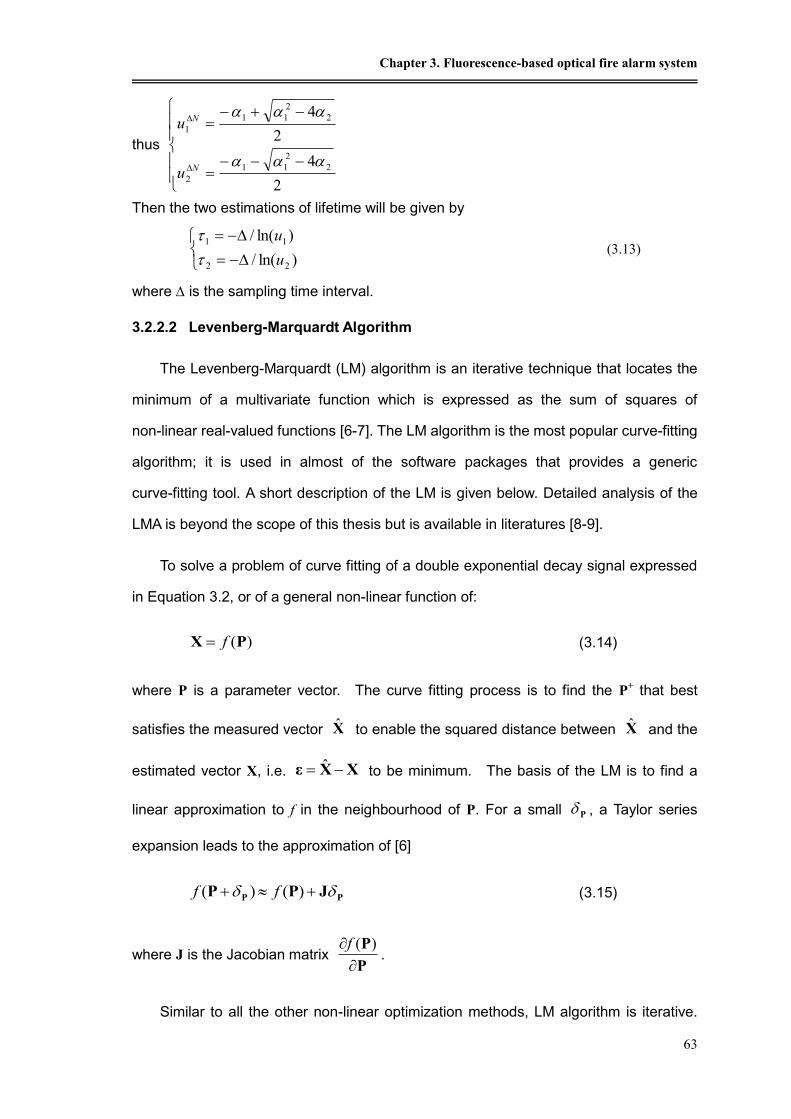
Chapter 3. Fluorescence-based optical fire alarm system
63
thus
Then the two estimations of lifetime will be given by
(3.13)
where is the sampling time interval.
3.2.2.2 Levenberg-Marquardt Algorithm
The Levenberg-Marquardt (LM) algorithm is an iterative technique that locates the
minimum of a multivariate function which is expressed as the sum of squares of
non-linear real-valued functions [6-7]. The LM algorithm is the most popular curve-fitting
algorithm; it is used in almost of the software packages that provides a generic
curve-fitting tool. A short description of the LM is given below. Detailed analysis of the
LMA is beyond the scope of this thesis but is available in literatures [8-9].
To solve a problem of curve fitting of a double exponential decay signal expressed
in Equation 3.2, or of a general non-linear function of:
(3.14)
where P is a parameter vector. The curve fitting process is to find the P+ that best
satisfies the measured vector to enable the squared distance between and the
estimated vector X, i.e. to be minimum. The basis of the LM is to find a
linear approximation to f in the neighbourhood of P. For a small , a Taylor series
expansion leads to the approximation of [6]
(3.15)
where J is the Jacobian matrix .
Similar to all the other non-linear optimization methods, LM algorithm is iterative.
2
4
2
4
2
2
11
2
2
2
11
1
N
N
u
u
)ln(/
)ln(/
22
11
u
u
)(PX f
X̂ X̂
XXε ˆ
P
PP JPP )()( ff
P
P
)(f

Optical fibre high temperature sensors and their applications
64
Initiated at the starting point P0, the method produces a series of P1, P2 … that converges
towards a local minimizer for f. At each iteration step, it is required to find a that can
minimize the square of . The sought is
thus the solution: the minimum is attained when it is orthogonal to the column space of J.
Thus this leads to , where JT is the transposition of J, which yields as
the solution of the so-called normal equations [6]:
(3.16)
The matrix in the left hand side of Equation 3.16 is the approximate Hessian,
i.e. an approximation to the matrix of second order derivatives.
The LM algorithm actually solves the equation by a 'damped version' of Equation
3.16, known as the augmented normal equations
(3.17)
where the off-diagonal elements of N are identical to the corresponding elements of
and the diagonal elements are given by
(3.18)
This strategy of altering the diagonal elements of is called damping and u is
referred as the damping term (or damping factor).
In each iteration step of LM algorithm method, the parameter vector P is replaced
by a new estimate , if the updated parameter vector with calculated
from Equation 3.17 leads to a reduction in the error of , the update is
accepted and the process repeats with a decreased damping term. Otherwise, the
damping factor is increased, the augmented normal equations are required to be solved
again and the process iterates until a value of that decreases is found.
The process of repeatedly solving Equation 3.17 for different values of the damping
P
PPP JεJPXPX )(ˆ)(ˆ ff P
0)( εJJ PT
P
εJJJ P
TT
JJT
εJN P
JJT
ii
T
ii u )( JJN
JJT
PP PP P
XXε ˆ
P XXε ˆ

Chapter 3. Fluorescence-based optical fire alarm system
65
term continues until an acceptable update to the parameter vector is found that leads to
one iteration of the LM algorithm. The LM algorithm terminates when at least one of the
following conditions is met, and the last parameter vector P is considered to be the
solution [6]:
The magnitude of the gradient of , i.e. in the right hand side of
Equation 3.16 drops below a threshold.
The relative change in the magnitude of drops below a threshold.
The error drops below a threshold.
A maximum number of iterations is completed
For the fire alarm system, a four parameter Vector P=(A1,B1, A2,B2) can be used to
represent the following measured double exponential decay using LM algorithm:
(3.19)
where and .
For a double-exponential regression, the Double-Prony method offers a fast
solution, however the Levenberg-Marquardt Method gives higher accuracy, but at a cost
of longer computing time due to its algorithm complexity. In this work, the latter method
was used for high accuracy measurement after a preliminary comparison of this two
algorithms using a commercial simulation software package of Matlab. The detailed
procedure of the LM algorithm is programmed in the interface software using Delphi Ver.
6.0, though its detail is not present in this thesis due to the complex nature of the
program, which is part of the whole Delphi project of the system, and the limitation of the
space of the thesis.
3.2.3 Solutions to the fire alarm system signal processing
The determination of the hotspot temperature, and thus the decay time associated
εεT
εJT
P
εεT
)exp()exp()( 2211 tBAtBAtf
1
1
1
B
2
2
1
B

Optical fibre high temperature sensors and their applications
66
with that requires the de-convolution of that signal from the background. With the added
problem of non-linearity of the observed signal, it is difficult to obtain the temperatures
corresponding to the background and to the hotspot directly from the original signal
using Equation 3.2, and a modified signal processing approach is required. In this work,
two different methods, termed as the correction method and the lifetime adjustment
method, were introduced and implemented to solve the problem and obtain comparative
data.
3.2.3.1 Correction method
The correction method aims to transform the obtained complex signals into near
ideal ones, which can then be further processed by the use of equations 3.1-3.3.
When the Nd-fibre experiences a uniform temperature, the observed signal, ,
can be adjusted to be an ideal single exponential through the following modification
(3.20)
where is the lifetime obtained by fitting the actual signal with single exponential,
is the corresponding ideal single exponential signal, and is the
experimental correction factor given by
(3.21)
which can be derived from a curve fitting of the observed signal and the ideal
signal when the entire fibre is exposed to an uniform temperature. Once the
correction factor is obtained, the same correction factor is then used for the rest of
measurement, either with or without the presence of a hotspot.
When there is a hotspot, the received signal is adjusted by the correction factor to
achieve a double exponential signal.
(3.22)
),( tf
),(/),(),( thtftf
),( tf ),( th
),(/),(),( tftfth
),( tf
),( tf
),(/),,(),,( 2121 thtftf

Chapter 3. Fluorescence-based optical fire alarm system
67
where is the actual received signal, and is the corrected signal.
is the lifetime of single exponential fitting of the signal , and is the
corresponding correction factor of .
After correction, can be processed using Equation 3.2 to obtain two
values of the lifetimes (1, 2), which are related to the corresponding temperatures (T1,
T2) by Equation 3.3.
However, the correction method has demonstrated certain limitations and they are
listed below
The best suited correction factor is difficult to be obtained under the
wide range of conditions of this experiment (temperature ranges of both the
hotspot and the background)
The accuracy of the calibration obtained is poor
3.2.3.2 Lifetime Adjustment Method
In view of the difficulty of obtaining a suitable correction factor and other
problems in the system using the above approach, such as the sensitivity to the
fluctuations of LD light intensity, a second approach, i.e. lifetime adjustment method,
was introduced and discussed in this section.
In this method, no correction factor is involved, and instead all the decay signals
were treated as double exponentials, no matter whether a hot spot is present or not.
Thus two lifetimes (1, 2) are obtained, and two temperatures are derived. The
temperatures are calculated using Equation 3.3 directly from lifetime (1, 2). Then they
are adjusted according to a predefined initial lifetime set of ( , ), and this approach
is thus termed as Lifetime Adjustment Method and described as follows.
As an initial condition, in the absence of a hotspot, the initial values, 0 from a single
exponential fitting and , from a double-exponential fitting are obtained
),,( 21 tf ),,( 21 tf
),,( 21 tf ),( th
),,( 21 tf
),( th
),( th
0
10
2
0
10
2

Optical fibre high temperature sensors and their applications
68
respectively from the fluorescence signal. Thus the initial temperature T0 was obtained
from lifetime 0, and, as there is no hot spot present at the initial condition, the lifetimes
, obtained from the same fluorescence signal using double-exponential fitting,
should respond to the same temperature value of T0. Given a uniform temperature
background, the following conditions are satisfied
(3.23)
where the functions, , , are predefined through an initial calibration of
the experimental data.
At any other temperature, weather a hot spot is present or not, the lifetimes 1 and
2 interpreted from the double-exponential signal fitting, may be transformed to
represent their corresponding temperatures T1 and T2, after the adjustment using the
initial values of
(3.24)
(3.25)
where A0, A1, A2, and B0, B1, B2 are the calibration parameters from experiments.
A series of more complex calibration functions, shown in Equation 3.26 and 3.27,
may be required to achieve a higher accuracy, especially under the circumstances with
a varying background.
(3.26)
(3.27)
The correlation functions, termed as G(1,2) and H(1,2) , are added to take into
account of the effect caused by the varying background.
0
10
2
0
0
20
0
1
0
0
)(,)(
)(
ThTg
fT
)(f )( 1g )( 2h
0
2
0
10 ,, T
20
112
0
11100
0
1110
0
111
0
1
0
1111
)()(
),(),()(),(
AAAT
FTFgFT
20
222
0
22100
0
2220
0
222
0
2
0
2222
)()(
),(),()(),(
BBBT
FTFhFT
),(])()([ 21
20
112
0
111001 GAAATT
),(])()([ 21
20
222
0
221002 HBBBTT

Chapter 3. Fluorescence-based optical fire alarm system
69
If the LD intensity fluctuation is taken into consideration, the above equations should
be modified as follows
(3.28)
(3.29)
where H(I) is the correction factor in relation to the fluctuation of the light source
intensity.
To implement this Lifetime Adjustment method requires the availability of a set of
predefined parameters and this can only be achieved through a series of pre-defined
experiments.
3.2.3.3 Flowcharts for the two methods
For comparison, the flowcharts of the data processing procedures for the two
methods are illustrated in Figure 3.1.
These two approaches used to provide a better signal processing and thus
enhance the performance of the fire alarm system. With preliminary tests and
evaluations, the lifetime adjustment method was observed to offer better performance,
in terms of accuracy, which is believed to be benefited from more experimental
calibration parameters being used. More details of the experimental tests will be
discussed in the following sections.
)},(])()([{)( 21
20
112
0
111001 FAAATIHT
)},(])()([{)( 21
20
222
0
221002 GBBBTIHT

Optical fibre high temperature sensors and their applications
70
Figure 3.1: Flowcharts of the two signal processing methods
3.3 Experimental setup of the fluorescence-based fire alarm system
3.3.1 Probe configuration
A one meter probe was prepared for the fire alarm system, as shown in Figure 3.2.
The probe consisted of one piece of Nd-doped fibre of 80 cm length, with the tips
connected to two pieces of plain glass fibres. The maximum length of the sensor fibre,
3-4 meters estimated, will be limited by the absorption of the fibre and the fluorescence
signal ration of that of hotspot to that of background. The Nd-fibre was placed in a one
meter steel tube for protection. Before being placed into the protective tube, the Nd-fibre
was annealed at 600°C for about 24 hours, as this had previously been seen as
important for stabilizing the performance of the fibre. The probe thus assembled can
endure temperatures up to 550°C (for continuous exposure) and 700~800°C (for a
pulsed temperature excursion), based on the test results of the fluorescence
characteristics of Nd doped fibres carried out by Zhang et al [10].
Data Acquistion
f(t,1,)
Single-exponential fitting
(IAverage,Average)
Initialize
(10,2
0)
Calculate temperature
T1=f(1,0) T2=f(,
0)
Double-exponential fitting
(1,)
Data Acquistion
f(t,1,)
Single-exponential fitting
Initial I0,0
Double-exponential fitting
1, T1=f() T2=f()
Calculate correct factor
h(t)
Correct the signal
f '(t,1,)
Lifetime Adjustment Correction method

Chapter 3. Fluorescence-based optical fire alarm system
71
Figure 3.2: Assembly of a sensing probe
3.3.2 System setup
A schematic diagram of an optical fibre fluorescence-based fire alarm system,
using the 1m Nd-doped fibre probe described above as a sensing element, is illustrated
in Figure 3.3. Figure 3.4 shows the experimental setup of the fire alarm system
prototype in the laboratory. A 785 nm laser diode, whose output is modulated by a TTL
square wave, is used to pump the doped fibre at both ends through a 2×2 coupler.
Following the termination of the stimulation light, the fluorescence signal generated is
captured by an InGaAs PIN photo-detector from the other arm of the coupler.
Subsequently the captured fluorescence decay signal is digitalized and passed to a
computer via a PowerDAQ data acquisition card. An interface software program was
written and used to regress the digitalized fluorescence signal, and hence to obtain the
lifetimes and their corresponding temperatures, both of the background and of the
hotspot.
10cm
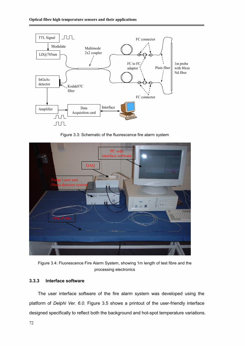
Optical fibre high temperature sensors and their applications
72
Figure 3.3: Schematic of the fluorescence fire alarm system
Figure 3.4: Fluorescence Fire Alarm System, showing 1m length of test fibre and the
processing electronics
3.3.3 Interface software
The user interface software of the fire alarm system was developed using the
platform of Delphi Ver. 6.0. Figure 3.5 shows a printout of the user-friendly interface
designed specifically to reflect both the background and hot-spot temperature variations.
Interface
Modulate
LD@785nm
Kodak87C
filter
Multimode
2x2 coupler
1m probe with 80cm
Nd fiber
FC to FC
adaptor
FC connector
InGaAs
detector
FC connector
Plain fiber
TTL Signal
Amplifier Data
Acquisition card
Pump Laser and
Photo detector system
Fibre Probe
DAQ
PC with
interface software

Chapter 3. Fluorescence-based optical fire alarm system
73
The software was designed to control and access the data acquisition card, read data
from the card. It was programmed to calculate the lifetimes using
Levenberg-Marquardt Algorithm for double exponential data fitting from the digitalized
fluorescence signal (after being adjusted by a correction factor, or after the resulted
lifetimes having been adjusted), and derive and display the corresponding temperatures,
of the background and of the hotspot.
The program was built with a function of self-calibration, which is carried out
automatically under certain pre-set conditions using the experimental data obtained
during the evaluation. This is essential to minimize the influence of the signal intensity
variation and several other potential system errors.
The interface software also provides some additional functions, such as data
management, providing a user-friendly graphic and datasheet presentation of the
measurement, etc.
3.4 Tests and evaluations of the fluorescence-based fire alarm system
The fluorescence-based fire alarm system developed has undergone some tests
Figure 3.5: Printout from the interface software – fluorescence-based fire alarm system

Optical fibre high temperature sensors and their applications
74
and evaluations in the laboratory. The results are presented below, some of which were
obtained during the system development period.
3.4.1 Simulated experimental results
A simulated experimental system, as illustrated in Figure 3.6, was established to
test the signal processing method, under different temperatures generated in the
laboratory. Two ovens were used to simulate the hotspot and the background
individually and separately. A tube oven, which operates up to 1200°C, provides the
hotspot, while a large cube oven, which operates up to 300°C, simulates the various
background circumstances.
As the 1m straight probe is protected by a stainless steel tube, it is difficult to vary
the background temperature with different hotspot temperatures. To offer some
flexibility, the simulated experimental setup described above is to use the 1 meter Nd
fibre for background temperature measurement and one piece of Nd-doped fibre around
8 cm length for the hot spot temperature measurement. In doing so the simulated fire
alarm system was able to test both the data acquisition system and the signal
processing method by varying background and hotspot temperatures. After a certain
correction factor was determined and applied (correction method), the fluorescence
decay data were fitted to obtain two lifetimes corresponding to both the background and
Figure 3.6: Experimental arrangement for simulation
LD@785nm
Cube oven
Tube oven
1m Nd fiber Kodak87C
filter
Fiber coupler 4~9cm Nd fiber
InGaAs
detector
Plain fiber
Interface Amplifier Data
Acquisition card

Chapter 3. Fluorescence-based optical fire alarm system
75
the hotspot. The results are illustrated in Figure 3.7, which shows that an obvious
difference between the two lifetimes is observed when the difference of temperatures
between the background and the hotspot is larger than 100°C. But when the
temperature difference of them is less than 100°C, the lifetime difference of the
background and the hotspot is difficult to be distinguished.
Figure 3.7: Lifetimes obtained of simulative experiment vs. hotspot temperature at vary
background
3.4.2 System performance at a room temperature background
Following the above simulation tests, the fire alarm system with the 1 meter probe
was tested at room temperature. A heat-gun or a gas burner was used to provide the
hotspot over a spatial region of less than 100mm. The maximum operational
temperature of the heat-gun is about 350°C, and that of the gas burner is around
1100°C. The system was tested when the hotspot temperature varied from room
temperature up to a maximum continuous temperature of 550°C, with some short peak
temperatures of about 700~750°C. Both the correction method and the lifetime
adjustment method had been used in the test.
280
300
320
340
360
380
400
420
440
0 100 200 300 400 500 600
Hotspot temperature (°C)
Lif
etim
e ( �
s)
50°C Background
100°C Background
150°C Background
Simple temperature

Optical fibre high temperature sensors and their applications
76
For the correction method, the typical response time was about 5 seconds (using
HPVV as interface software program platform, and may vary with different computers).
A hotspot could be determined when it lasted for more than 2~3 s (heated for 2~3 s with
a heat-gun or gas burner). In the tests, it was noticed that the system missed some
“transient” hotspots (heated for less than 1 second by passing through the heat gun
over the probe). The method also had the problem with the measured values of the
background and the hotspot temperatures. When there was a hotspot along the probe,
the background temperature dropped dramatically while the hotspot temperature rises,
as shown in Figure 3.8.
Given the problems arising with the correction method, the lifetime adjustment
method is found to be more suitable for the application to improve the performance of
the system, as discussed below.
When using lifetime adjustment method, almost every rapidly appearing hotspot, e.g.
from a sweeping of the heat gun or the burner behind the probe, could be picked up.
The typical response time is about 2 seconds (with the same computer), as shown in
Figure 3.9. After the system being calibrated using Equation 3.24 and Equation 3.25, it
was observed that , at room temperature with the hotspot temperature varying from
Figure 3.8: Response of hotspot at room temperature background-- Correction method
-20
0
20
40
60
80
100
120
140
0 50 100 150 200 250
Time (second)
Tem
pera
ture
(°C
)
Hotspot Background Average temperature
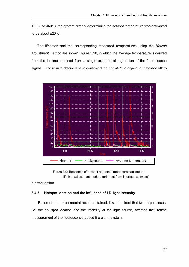
Chapter 3. Fluorescence-based optical fire alarm system
77
100°C to 450°C, the system error of determining the hotspot temperature was estimated
to be about ±20°C.
The lifetimes and the corresponding measured temperatures using the lifetime
adjustment method are shown Figure 3.10, in which the average temperature is derived
from the lifetime obtained from a single exponential regression of the fluorescence
signal. The results obtained have confirmed that the lifetime adjustment method offers
a better option.
3.4.3 Hotspot location and the influence of LD light Intensity
Based on the experimental results obtained, it was noticed that two major issues,
i.e. the hot spot location and the intensity of the light source, affected the lifetime
measurement of the fluorescence-based fire alarm system.
Figure 3.9: Response of hotspot at room temperature background
-- lifetime adjustment method (print-out from interface software)
—— Hotspot —— Background —— Average temperature

Optical fibre high temperature sensors and their applications
78
Hotspot location influence
The influence of the hot spot location has been investigated. When the probe was
heated by the heat-gun, which was set at a constant temperature but at different
positions along the probe length, different responses were observed, as shown in
Figure 3.11. Firstly, the two ends of the probe were more sensitive to the hotspot
temperature change than the middle of it, the derived hot spot temperature readings at
the ends and at the middle of the fibre have shown a difference of some 70oC, when the
actual hot spot temperatures are almost the same. This is because the signal change is
more significant when the fibre ends are heated up compared to that in the middle.
Secondly, as the 2×2 coupler is not absolutely 50:50 in its intensity division, therefore
the sensitivities at both ends are slightly different.
Figure 3.10: Measured temperatures vs. hotspot temperature at room temperature background
0
100
200
300
400
500
0 100 200 300 400 500
Hotspot temperature (℃)
Mea
sure
d T
emp
erat
ure
(℃)
Hotspot
Background
Average temperature

Chapter 3. Fluorescence-based optical fire alarm system
79
Figure 3.11: Position sensitivity of the fire alarm system (At room temperature background and
200oC hotspot)
LD light intensity influence
Another issue is the fluctuation of the LD light intensity which induces the initial
intensity variation of the fluorescence decay signal generated. It has shown a
substantial effect on the temperature (fluorescence lifetime) measured. While keeping
the 1 meter probe under a constant ambient temperature, the fluorescence intensity
was changed by an optical adjustable attenuator, and the corresponding temperature
readings at different intensity were recorded. The results are shown in Figure 3.12. The
measured temperature had a maximum fluctuation of 8oC when the fluorescence
intensity is changed from 4.3 to 4.9 voltage. This suggests the importance of adding an
intensity factor in the calibration function, and thus using Equation 3.26 and Equation
3.27 for the lifetime adjustment.
0
100
200
300
0 20 40 60 80 100
Distanct from one end of the probe (cm)
Measu
red
Tem
pera
ture
(°C
)
HotSpotBackgroundAverage

Optical fibre high temperature sensors and their applications
80
Figure 3.12: Intensity sensitivity of the fire alarm system (At room temperature background in
absence of hotspot)
3.5 Summary and Conclusions
The fire alarm system, based on fluorescence lifetime measurement using data
fitting method, has demonstrated the potential of their applications in aero industry. In
summary, the fire alarm system developed has shown acceptable performance, with the
main specifications of system highlighted below having been met by using the lifetime
adjustment method approach.
Table 3-1: Specification of the fluorescence based fire alarm system
Typical response time ~2 seconds
Precision of measurement Background: ±5~10 °C
Hotspot: ±10~20 °C
Temperature Range Background: room temperature up to 350°C
Hotspot: room temperature up to 500°C
However the system has also demonstrated some limitations which are required to
be overcome and these include the dependence of the signal processing on the laser
power stability and the sensitivity to the location of hot spots. If the sensing length is
required to be extended from 1m to 3m, it involves a series of changes being made,
15
17
19
21
23
25
27
29
31
4.2 4.4 4.6 4.8 5
Intensity (V)
Measu
red
Tem
pera
ture
(°C
)HotSpotBackgroundAverage

Chapter 3. Fluorescence-based optical fire alarm system
81
mainly as followings:
Higher power LD pumping source
A pumping source with a central wavelength which is not matching with the
absorption peak wavelength of Nd-doped fibres to avoid absorption saturation
Neodymium fibres with lower doping concentrations.
In light of the above issues and the challenges arising, a more practical sensing
system, using arrays of fibre Bragg gratings, has been developed and will be discussed
in detail in Chapter 5.
References
[1]. T. Sun, K. T. V. Grattan, W. M. Sun, et. Al., “Rare-earth doped optical fiber approach to
an alarm system for fire and heat detection”, Review of Scientific Instruments, vol. 74,
2003, pp. 250-255
[2]. T. Sun, Z. Y. Zhang, K. T. V. Grattan, “Frequency-domain fluorescence based fiber
optic fire alarm system”, Review of Scientific Instruments, vol. 72, 2001, 2191-2196
[3]. T. Sun, Z. Y. Zhang, K. T. V. Grattan, and A. W. Palmer, “Determination of local high
temperature excursion in an intrinsic doped fiber fluorescence-based sensor”, Review
of Scientific Instruments, vol. 69, 1998, 2930-2934()
[4]. Fire Fighting, Extinguishing, Protection and Detection Products, http://www.kidde.com
[5]. T. Sun, Z. Y. Zhang, et al., “Analysis of double exponential fluorescence decay
behavior for optical temperature sensing”, Review of Scientific Instruments, vol. 68,
1997, pp.58-65;
[6]. K. Levenberg, “A Method for the Solution of Certain Non-linear Problems in Least
Squares”, Quarterly of Applied Mathematics, vol. 2(2), 1944, pp.164–168
[7]. D.W. Marquardt, “An Algorithm for the Least-Squares Estimation of Nonlinear
Parameters”, SIAM Journal of Applied Mathematics, vol. 11(2), 1963, pp.431–441
[8]. O. Nelles, “Nonlinear system identification”, §4.5, Springer, 2001.
[9]. W. T. Vetterling, “Numerical recipes example book (C)”, §15.5, Cambridge University
Press, 1992
[10]. Z. Y. Zhang, K. T. V. Grattan, A. W. Palmer, and B. T. Meggitt, “Spectral characteristics
and effects of heat treatment on intrinsic Nd-doped fibre thermometer probes”,
Review of Scientific Instruments 69, 1998, pp.139-145

Optical fibre high temperature sensors and their applications
82

Chapter 4. Strong Fibre Bragg gratings for high temperature sensor applications
83
Chapter 4. Strong Fibre Bragg gratings for high
temperature sensor applications
4.1 Introduction of Fibre Bragg grating
A fibre Bragg grating (FBG) is a type of distributed Bragg reflector constructed in a
short segment of optical fibre that reflects a particular wavelength of light and transmits
all others. This is achieved by creating a periodic variation in the refractive index of the
fibre core, as shown in Figure 4.1 [1].
For a conventional FBG, the periodicity of the index modulation has a physical
spacing and when light is launched into the grating and the Bragg reflection condition [1]
between the grating planes and incident light is satisfied, a narrow band spectrum,
centred at Bragg wavelength, B, of the incident light is reflected back. The Bragg
wavelength of the grating, can be represented by:
effB n2 (4.1)
Figure 4.1: Structure of a fibre Bragg grating

Optical fibre high temperature sensors and their applications
84
where neff is the effective refractive index of the fibre core, and is the grating spacing of
the refractive index modulation.
The fibre Bragg grating can work as a wavelength specific dielectric mirror.
Therefore, a fibre Bragg grating can be used as an inline optical filter to block certain
wavelengths, or as a wavelength-specific reflector. The wavelength of the reflected
narrow bandwidth of light responds also to changes in temperature and strain, thus the
FBG can be used as a sensing element. Up to a few thousands of FBG sensors can
be recorded into a single optical fibre and interrogated simultaneously with a single
instrument [1] - the effect offers a very low-cost option for distributed monitoring of strain
and/or temperature within large structures. The suitability of FBGs for structural health
monitoring has been widely reported [2,3]. Since the first discovery of the FBG, the
invention of it has revolutionized the fields of telecommunication and sensing, and has
led to numerous applications in these fields[4,5]..
4.1.1 Short History of fibre Bragg gratings
The first observations of photosensitivity and index of refraction changes in
germanosilica fibres were reported by Hill and co-workers at the Communication
Research Centre (CRC), Canada, in 1978 [6,7]. During an experiment carried out to
study the nonlinear effects in a specially designed optical fibre with heavy germanium
dopant, the visible light from an argon ion laser (= 488 nm) was launched into the core
of the fibre, under a prolonged exposure, an increase in the attenuation of the fibre was
observed, and it was noticed that the intensity of the back reflected light from the fibre
increased significantly with exposure time. This increase in reflectivity was recognized
as a result of a permanent refractive-index grating, thought to be very weak in an order
approximately of 10-6, being photo-induced in the fibre, which resulted in a narrow-band
reflection at the writing wavelength.
In their experiment, the refractive-index perturbation of the fibre was formed as a
result of a standing wave intensity pattern being formed by the 4% Fresnel back
reflection at the far end and the forward-propagating light. This refractive-index grating

Chapter 4. Strong Fibre Bragg gratings for high temperature sensor applications
85
acted as a distributed reflector that coupled the forward propagating light to the counter
propagating light beams. This coupling of the beams provided positive feedback, which
enhanced the strength of the back-reflected light, and thereby increased the intensity of
the interference pattern, which in turn increased the index of refraction at the high
intensity points. This process was continued until eventually the reflectivity of the grating
reached a saturation level. These gratings were, thus, called self-organized or
self-induced gratings since they formed spontaneously without human intervention. The
periodic refractive index perturbation in a meter or so of fibre formed a Bragg grating
with a bandwidth being around 200 MHz.
This new nonlinear photorefractive effect in optical fibres was called photosensitivity.
The importance of this discovery in potential applications was recognized even at that
time. However, the discovery did not bring a significant technical breakthrough for nearly
a decade. The main reason for this is believed to be the difficulty in repeating the set-up
of the original experiments, and it was thought the observations were confined only to
the "magic fibre" at CRC.
Although the discovery of the photosensitivity played a key role in the
advancements of optical fibre technology, devices such as the self-induced gratings,
demonstrated by Hill et al [7], were not practical, primarily due to the Bragg resonance
wavelength being limited by the argon ion laser writing wavelength (488nm). The
major breakthrough came with the report on the side writing technique using
single-photon absorption at 244 nm by Meltz et al [8] almost a decade later. They
demonstrated reflection gratings in the visible part of the spectrum (571-600 nm) using
two interfering beams external to the fibre. The wavelength of Bragg condition can be
altered by changing the angle between the interfering beams. This side writing
technique provides the much-needed degree of freedom to shift the Bragg resonance to
longer and useful, almost any, wavelength, such as 1530 nm, permitting their use in
modern communications and many other applications.
In the last two decades, groups worldwide achieved breakthroughs in direct optical
inscription of high-quality gratings into the core of optical fibres using various techniques

Optical fibre high temperature sensors and their applications
86
such as the interferometric, phase mask, and point-by-point exposure to ultraviolet laser
light. Gratings with a wide range of bandwidths and reflectivity can be formed on time
scales ranging from a few nanoseconds (duration of the laser pulse) to a few minutes,
depending on the characteristics required. These gratings are low-loss in-line fibre
devices that can be written into the core non-invasively when and where desired,
offering narrow-band wavelength selection to precise specifications.
4.1.2 Types of Fibre Bragg gratings
4.1.2.1 Uniform Fibre Bragg gratings
Fibre Bragg gratings can be classified into three distinct formation regimes
according to the fabrication procedure and conditions, and they are type I, type IIA, and
type II gratings respectively.
Type I
Type I gratings are generally formed into most photosensitive fibres when exposed
to continuous wave (CW) or low frequency pulse UV radiation at a relatively low energy.
As seen in the transmission and reflection spectra of a type I grating exposed under a
broadband light source, a fundamental characteristic of this type of grating is that the
reflection spectrum of the guide mode is complementary to the transmission signal,
implying that there is negligible loss due to the absorption or reflection into the cladding.
Type I gratings, written into some photosensitive fibres, normal highly germanium
doped silica fibre, can be erased at a relatively low temperature (~300 oC) due to this
photosensitivity type of the grating. However, type I gratings writing into some other
photosensitive fibres may have higher sustainable temperature. Nevertheless, the type I
gratings are the most used gratings, and operate effectively in the temperature regime
from -40 oC to 80 oC, a temperature that satisfactorily covers most telecommunication
and sensor applications.
Type II
While gratings formed at low energy intensity are referred as type I gratings, another
Chapter 4. Strong Fibre Bragg gratings for high temperature sensor applications
87
type of grating is formed when the energy intensity of the writing light beam exceeds
over approximately 30 mJ [9]. This type of grating is termed as type II grating, which is a
damage grating physically caused in the fibre core on the side of the writing beams
under a single pulse exposure. Type II gratings usually have an irregular reflection
spectrum due to the non-uniformities of the excimer laser beam profile. By spatially
filtering the beams, type II gratings with better reflection profile, but with reduced
reflectivity, can be created. One main characteristic of this type of gratings is their
extreme stability at elevated temperatures [9]. No degradation in the grating reflectivity
was observed at 800oC over a period of 24 hours. This extreme temperature stability
can be utilized for sensing applications in some harsh environments. Another attractive
feature of the type II gratings is that the highly reflective gratings can be formed in a few
nanoseconds (the duration of a single laser pulse), suitable for large-scale mass
production of strong gratings. They can also be inscribed during the drawing process
before application of the protective coating.
Type IIA
Type IIA grating represents another type of grating formed in non-hydrogen-loaded
photosensitive fibres. Type IIA gratings are inscribed at low power densities through a
long exposure of approximately 30 minutes (depending on the fibre type and the
exposure beams), following type I grating inscription[10,11].It was found that the type
IIA gratings had dramatically improved temperature stability over the type I gratings.
Type IIA grating is able to withstand a higher temperature than the original Type I
gratings, a noticeable grating erasure by high temperature is observed only at the
temperatures over 500oC[10]. Clearly, the type IIA gratings are not very practical in
terms of fabrication. However, the improved temperature stability is very useful if the
system is exposed to high ambient temperatures in some applications.
All the above three different types of gratings are uniform in structure as illustrated in
Figure 4.2, where the grating planes along the whole grating are equally spaced and
identical to each other. There are other types of non-uniformly structured fibre gratings,
such as tilting gratings, chirped gratings, etc.
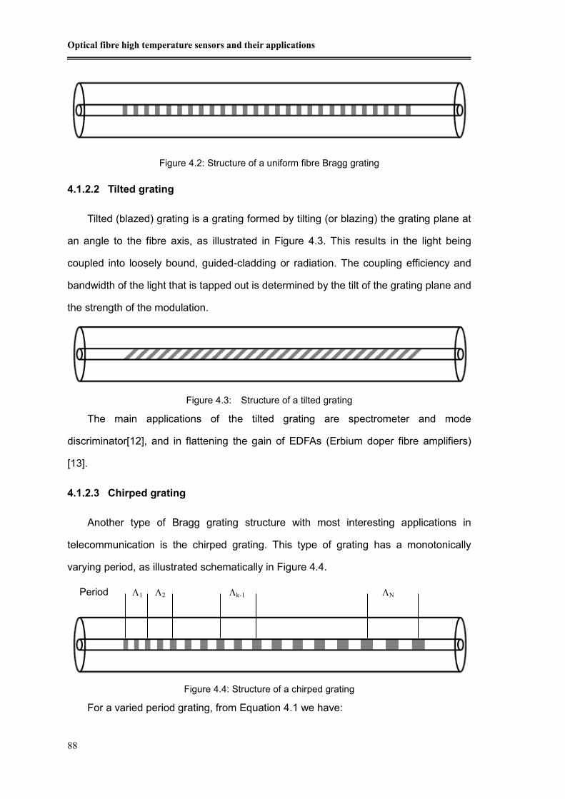
Optical fibre high temperature sensors and their applications
88
Figure 4.2: Structure of a uniform fibre Bragg grating
4.1.2.2 Tilted grating
Tilted (blazed) grating is a grating formed by tilting (or blazing) the grating plane at
an angle to the fibre axis, as illustrated in Figure 4.3. This results in the light being
coupled into loosely bound, guided-cladding or radiation. The coupling efficiency and
bandwidth of the light that is tapped out is determined by the tilt of the grating plane and
the strength of the modulation.
The main applications of the tilted grating are spectrometer and mode
discriminator[12], and in flattening the gain of EDFAs (Erbium doper fibre amplifiers)
[13].
4.1.2.3 Chirped grating
Another type of Bragg grating structure with most interesting applications in
telecommunication is the chirped grating. This type of grating has a monotonically
varying period, as illustrated schematically in Figure 4.4.
Figure 4.4: Structure of a chirped grating
For a varied period grating, from Equation 4.1 we have:
Figure 4.3: Structure of a tilted grating
1 2 k-1 N Period

Chapter 4. Strong Fibre Bragg gratings for high temperature sensor applications
89
)()(2)( zznz effB (4.2)
The simplest type of the chirped grating structures is the one in which the variation
in the grating period is linear:
zz i 0)( (4.3)
where is the starting period, and is the linear change of the period along the length
of the grating. This type of chirped grating structures can be considered as it is made up
of a series of smaller lengths of uniform Bragg gratings with increased period. If properly
designed, this type of structure can be used as a broadband reflector, which is useful in
both telecommunication and sensor applications.
4.2 Applications of fibre Bragg Gratings
Since the innovation of the fibre Bragg gratings, they have been extensively used in
telecommunications due to their unique filtering properties and versatility as in-fibre
devices. Bragg gratings have also been widely utilized as in-fibre sensors for many
applications as the Bragg wavelength of gratings responses directly to the temperature
or/and stain perturbations. In this section, the applications of FBGs in communication
and sensor systems are briefly summarized.
4.2.1 Applications in communication
Fibre Bragg gratings have emerged as important components in various lightwave
applications in telecommunication. Many in-fibre devices deploying fibre Bragg gratings,
such as fibre lasers, wavelength division multiplexers and demultiplexers, Raman
amplifiers, remote pumping amplifiers, dispersion compensators, and gain equalisers,
have been demonstrated and developed for the applications in communication [14-24].
As these device arising from these applications in telecommunications are also widely
used as sensor system components, the following section will briefly describe some of
these applications
4.2.1.1 Fibre laser
Fibre lasers have been widely used in the telecommunication systems to meet the

Optical fibre high temperature sensors and their applications
90
increasing demand of high speed and high capacity transmission, as they offer great
advantages of being easily integration into the basic fibre communication systems. The
development of fibre Bragg gratings has further enhanced the functionality of fibre
lasers.
An example of a simple erbium-doped fibre laser configuration is schematically
illustrated in Figure 4.5 [14]. In this fibre laser, the laser cavity consists of a 2-meter long
erbium-doped fibre with Bragg gratings at each end for providing feedback. The output
coupler has a narrow band grating of around 80% reflectivity with 0.12nm linewidth. The
broadband mirror was formed by a series of narrowband gratings, which nowadays can
be easily replaced by a single broadband grating, such as a chirped grating. The fibre
laser output is at the wavelength of the narrowband output coupler Bragg grating, when
pumped at 3.0 mW, while the lasing threshold of the laser was 0.5 mW.
Figure 4.5: Schematic of an erbium-doped fibre laser with Bragg gratings at each end providing
feedback to the laser cavity
Other fibre lasers utilising fibre Bragg gratings, such as with multi-wavelength
operation lasers [15], single-mode/single frequency fibre lasers [16,17], mode-locked
fibre lasers [18], and fibre Raman laser [19] have also been reported for
telecommunication applications.
4.2.1.2 Fibre amplifiers
Erbium doped fibre amplifiers (EDFAs) are a device which has received the most
attention in the modern lightwave communication systems. They have significantly
changed the future of optical communications. Fibre Bragg gratings have been wide
Ti:Sapphire laser
Power Meter
Neutral density filter
Beam Splitter
Erbium doped fibre
Broadband Bragg Mirror
Output coupler Bragg Grating
Output
Objective

Chapter 4. Strong Fibre Bragg gratings for high temperature sensor applications
91
deployed in the EDFAs as a selective reflector for the signal and pump light. Over the
last several years, fibre Bragg gratings have been designed and optimized to
dramatically improve the performance of EDFAs, for example for pump laser
wavelength stabilisation, pump reflectors, and gain wavelength flattening. Fibre Bragg
gratings have therefore become an important integral part of EDFA for tailoring its
performance.
Figure 4.6 shows several configurations that have been proposed for fibre amplifiers
utilising fibre Bragg grating reflectors to improve performance [20]. For instance, by
placing a fibre Bragg grating as a broadband reflector at the output of EDFA, it can
increase the small-signal gain and efficiency by recycling the remnant pump light. The
fibre grating can also act as a wavelength selective reflector that discriminates between
the signal and the pump light, thus increasing the saturated output power.
Figure 4.6: Configurations of reflected pump and signal in EDFA.
Reflection by gratings nearly doubles the small signal gain and increases saturated output power
(after [20])
4.2.1.3 Wavelength Division Multiplexers/Demultiplexers
The rapid growth in the use of phones, internet, etc, has increased the volume of
telecommunication traffic enormously. The capacity of long-distance telecommunication
Signal Signal
Signal Signal
Signal Signal
Pump Pump
Pump Pump
Pump
Pump
Output Output
Output Output
Output Output
Er fibre Er fibre
Er fibre Er fibre
Er fibre Er fibre
Signal reflector
Pump reflector
Signal and pump reflector
Signal reflector
Signal reflector
Pump reflector
Pump reflector

Optical fibre high temperature sensors and their applications
92
links had to increase to keep the pace with it. Wavelength division multiplexer (WDM),
which allows multiple wavelengths to carry multiple optical signals in a single fibre
simultaneously, is a promising and widely used device to enhance the capacity of
modern optical fibre communication links.
WDMs utilising fibre Bragg gratings have been studied and developed by many
researchers. One of the earliest demonstrations of this technique is reported by Mizrahi
[21]. The operational principle of this WDM is illustrated in Figure 4.7a. It consisted of a
1x4 fused fibre splitter in conjunction with a fibre grating transmission filter in each of the
output ports. The filters were designed to pass the signal wavelength of each port while
rejecting the other three channels. The fibre transmission filter was formed by pairing
two gratings that do not have any overlap in wavelengths, which makes it possible to
create a simple band-pass filter, in which the two gratings reject a broad range of
wavelengths, but the desired wavelengths pass through unaffected between the grating
stopbands. The test result of this device of a high-resolution measurement is shown in
Figure 4.7b. The signal wavelength space of the channels of the WDM was around 200
GHz (~1.6 nm intervals). The peak attenuation of the filter was measured to be over 80
dB, which resulted in excellent crosstalk performance.
(a) (b)
Figure 4.7: Schematic illustration of a four channel fibre grating WDM. The plot (b) shows a high
resolution measurement of a complete demultiplexers system for one of the channels (after [21])
There are many other devices used in communications, such as dense wavelength
division multiplexers (DWDM) [22], dispersion compensation devices[23], optical fibre
1
2
3
4
1x4 fused
Fibre splitter

Chapter 4. Strong Fibre Bragg gratings for high temperature sensor applications
93
phase conjugators[24], in which the fibre Bragg gratings are employed. They will not be
discussed here as they are beyond the research of this thesis. Readers are referred to
text books, e.g. by Othonos [3], for more detailed information.
4.2.2 Applications in optical fibre sensors
As the Bragg wavelength of fibre Bragg gratings is changed with the perturbation
applied on the grating, fibre gratings have been considered as excellent sensing media
since the earliest stage of their development. Sensor systems based on fibre Bragg
gratings have been reported to measure static and dynamic measurands, such as
temperature, strain, pressure, and some chemicals [5,26-34]. One of the major
advantages of such FBG-based sensor systems is the transmitted signal is the
wavelength-encoded which makes the sensor independent of signal intensity variations,
e.g. due to the fluctuating light source power level and connector insertion losses etc.
Moreover, FBG based sensors can be easily multiplexed, making a promising sensor
network for large structure measurement. Since the innovation of fibre Bragg gratings,
FBG-based sensors have been widely applied in the field of civil structure monitoring,
aerospace industries, off-shore engineering, process control, and medical applications.
4.2.2.1 Optical sensing mechanism of fibre Bragg gratings
A fibre Bragg grating has an inherenet sensitivity to strain and temperature, as its
resonance wavelngth is dependent on the effective refractive index of the fibre core and
the grating period. Therefore gratings can be used for measurement of strain,
temperature, or some other measurands, by monitoring the Bragg wavelength shift.
By differentiating Equation 4.1, the wavelength shift of the Bragg wavelength (B)
is given by:
effeffB nn 22 (4.4)
Hence, the wavelength shift (B) due to strain and temperature changes can be
given by:
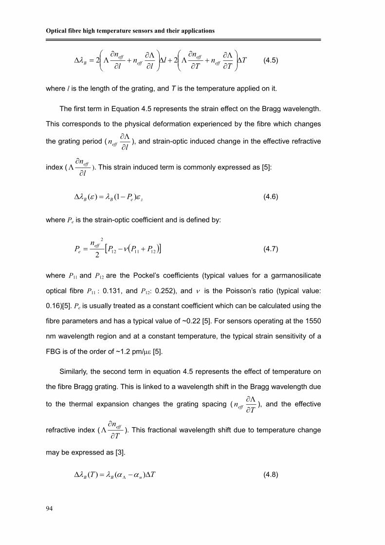
Optical fibre high temperature sensors and their applications
94
TT
nT
nl
ln
l
neff
eff
eff
eff
B
22 (4.5)
where l is the length of the grating, and T is the temperature applied on it.
The first term in Equation 4.5 represents the strain effect on the Bragg wavelength.
This corresponds to the physical deformation experienced by the fibre which changes
the grating period (l
neff
), and strain-optic induced change in the effective refractive
index (l
neff
). This strain induced term is commonly expressed as [5]:
zeBB P )1()( (4.6)
where Pe is the strain-optic coefficient and is defined by:
121112
2
2PPP
nP
eff
e (4.7)
where P11 and P12 are the Pockel’s coefficients (typical values for a garmanosilicate
optical fibre P11 : 0.131, and P12: 0.252), and is the Poisson’s ratio (typical value:
0.16)[5]. Pe is usually treated as a constant coefficient which can be calculated using the
fibre parameters and has a typical value of ~0.22 [5]. For sensors operating at the 1550
nm wavelength region and at a constant temperature, the typical strain sensitivity of a
FBG is of the order of ~1.2 pm/[5].
Similarly, the second term in equation 4.5 represents the effect of temperature on
the fibre Bragg grating. This is linked to a wavelength shift in the Bragg wavelength due
to the thermal expansion changes the grating spacing (T
neff
), and the effective
refractive index (T
neff
). This fractional wavelength shift due to temperature change
may be expressed as [3].
TT nBB )()( (4.8)

Chapter 4. Strong Fibre Bragg gratings for high temperature sensor applications
95
where
T
1 is the thermal expansion for the fibre (typically 0.55 x 10⁻⁶ for
silica fibre), and
T
n
n
eff
eff
n
1 represents the thermo-opto coefficient
(approximately 8.6 for germania-doped, silica core fibre). It is clearly shown that the
thermo-optic induced index change is the dominant effect. From equation 4.8, the
temperature sensitivity of a Bragg grating operating in 1550 nm region is expected to be
around 13 pm/oC [5], which may vary between different materials.
As shown in equation 4.5, the wavelength shift in the Bragg wavelength due to an
external perturbation to the grating, is the sum of the strain and temperature effect terms.
A crosstalk between these two effects is possible. Therefore, in many sensing
applications where only one measurand is of interest, it is necessary to deconvolute the
strain and temperature perturbations. In some cases, a simultaneous measurement of
strain and temperature is required.
4.2.2.2 Fibre Bragg grating sensor applications
Fibre Bragg grating based sensors have been continuously and rapidly developed
since they were first demonstrated for strain and temperature measurement about two
decades ago. In this section, a brief summary of the applications of FBG based-sensors
is addressed.
Applications in aerospace
The aerospace industry is very conservative where new development are
concerned, and all new sensors must undergo a long and rigorous testing period before
being accepted. However, Bragg grating sensor systems have shown potential for
aerospace applications as they cab be made into compact and lightweight temperature,
strain and pressure sensors compared to existing sensors already in use. Dunphy et
al. [26] presented a smart Bragg grating fibre sensor for monitoring of reinforced carbon
fibre composites (RCFCs) for curing and impact detection. Dunphy identified a
number of benefits arising from the combination of optical fibres and composites.

Optical fibre high temperature sensors and their applications
96
Interests of applications of Bragg grating sensors to space bound craft, where all
structures are subject to high acoustic and vibration loads to simulate the launch
conditions, have also been demonstrated. The Photonics Group at the NASA Ames
Research Centre designed specialized fibre Bragg sensor that could monitor the
condition of the cryogenic tanks aboard a Reusable Launch Vehicle [27]. The fibre
sensor was identified as an ideal candidate of embedded sensors for measuring strain
load on the cryogenic tanks (range 2500 , resolution 10 ), since fibre sensors
provided accurate data and being of a small size and lightweight, presenting no spark
hazard. Sensors are required to operate over a wide temperature range from -250 oC to
380 oC, in the application of space bound craft.
Applications in marine industry
Bragg grating sensors have great potential to be included in marine down-hole
instrumentation for exploring the natural oil resources, where conventional electronic
sensors cannot be used because of the extremely harsh marine environments.
In the late 1990s, Hjelme first used the fibre Bragg sensor for the characterization of
scaled marine vehicle models [28]. The system was designed to measure the slamming
forces between the wet deck and sea waves by locking the wavelength of the light from
a laser diode to the peak wavelength of a Bragg grating sensor mounted on the wet
deck of the vehicle model. The sensor had a dynamic range of 27 dB in a 1 kHz range.
Later on, a 16-channel system was developed for composite panel slamming test to
stimulate transient loading forces [29]. In the system, the grating sensors were attached
to the wet and dry side of the composite panel, which was mounted on a mechanical rig
loaded with weights exceeding 100 kg. The measurement results provided the
information of the survival characteristics of the grating sensors. The system
demonstrated a sub-10 /Hz1/2 resolution and a bandwidth of over 5 kHz for the
maximum ±1000 strain levels.
Applications in civil engineering
Structural health monitoring in civil and structural engineering has undergone

Chapter 4. Strong Fibre Bragg gratings for high temperature sensor applications
97
continuous growth over the last few decades. Exploring new sensing technologies in
these applications has led to many innovations and development in sensor systems.
Due to the harsh environments in the civil engineering industry, fibre Bragg grating
sensors offer a viable approach with a number of advantages over traditional sensors.
Novel FBG sensors have been developed and deployed on highway bridges to measure
dynamic strain, static strain [30-32], and for various engineering structural monitoring
[33-34]. Results of these studies indicate that, if properly packaged, FBG sensors can
survive the severe conditions associated with the construction environments of civil
infrastructure.
Medical applications of fibre Bragg sensors
Optical fibre sensors, as well as Bragg grating based sensors, have been used in
medical applications. FBG-based temperature sensors are particularly suitable for
medical applications, where conventional electrical thermometers are inappropriate.
Rao et al. [35,36]presented a novel temperature sensor system in early years of FBG
sensor research and development, utilising Bragg gratings for remote temperature
measurements in an NMR machine. The system achieved an measured resolution of
±0.2 oC with an accuracy of ±0.8oC, limited by the quality of the flitter PZT element.
Samset et al. [37] demonstrated a FBG based temperature sensor for soft tissue
measurement. The system was calibrated to the temperature range of –195.8°C to
100°C for temperature measurement during the process of freezing (cryoablation)
porcine liver in vivo. The system yielded a temperature profile with 6.5 mm spatial
resolution and 5 second temporal resolution.
Fisher et al [38] demostrated that the fibre Bragg sensor could be used in principle
to detect the high frquency ultasonic field, in line with the requirement of improved
safety of ultrasound for medical applicaions. Cowie and his co-workers[39], presented
fibre Bragg sensor used for tactile sensing for biomedical applications. A
two-dimensional sensing surface using the system was demonstrated, with potential
applications in human balance and gait analysis, capable of detecting simultaneously
the position and shape of an object placed upon it.

Optical fibre high temperature sensors and their applications
98
Other applications of fibre Bragg sensors
In addition to the above mentioned areas, Bragg grating sensors have also been
employed for nuclear environment monitoring[40], current measuremnent of power
transmission line [41,42], off-shore wind turbine strain monitoring[43], etc. The
FBG-based system developed by the author in this project, has been employed in
several field tests, such as bridge strain structural monitoring, high temperature
monitoring, automotive exhaust temperature measurement, etc. and further details are
presented in Chapter 5.
4.2.2.3 Advantages of fibre Bragg grating based sensors
Compared with other fibre-optic sensors developed and reported, fibre Bragg
grating sensors have shown a number of distinct advantages, such as:
The signal obtained from an FBG sensor is encoded directly in wavelength
which is, in general, an advantage over other sensing schemes as it is
intensity-independent and also facilitates wavelength division multiplexing
(WDM);
FBGs can be directly written into the fibre without changing the fibre diameter,
therefore making them suitable for conditions where small diameter probes are
required, for example, embedding sensors in advanced composite materials for
strain mapping or attaching to the human body for temperature profile.
The FBG sensor devices are simple, intrinsic sensing elements and have all the
advantages normally attributed to fibre sensors, such as electrically passive
operation, EMI immunity, high sensitivity, and potential low cost.
Another significant benefit that FBG sensors offer for remote monitoring is their
stability over time. Being a passive sensor, a FBG has zero drift and can be used
for many years with no need for recalibration. Indeed, it is practical to attach
sensors to bridges for instance and return with an instrument to interrogate the
sensors every few years to obtain a true picture of any structural movement

Chapter 4. Strong Fibre Bragg gratings for high temperature sensor applications
99
since the last reading. This further increases the economic advantage of the
technology since only one interrogation unit can service hundreds of structures
These advantages emphasize the important characteristics of FBGs, however,
FBGs are sensitive to both strain and temperature, therefore it is essential to address
this cross-sensitivity effect when they are used for specific applications. One key
problem for a practical system is the demodulation technique used to interrogate a small
Bragg wavelength shift as a function of the strain/temperature variation. Conventional
spectrometers or monochromators are not suitable for the measurement of Bragg
wavelength shifts as they are bulky, expensive and not robust enough for field
applications. In this work a practical FBG wavelength interrogation system together
with interface software for sensor applications has been developed, and the detail of it is
discussed further in Chapter 5.
4.3 Fabrication techniques of fibre Bragg gratings
Fibre Bragg gratings are created by "inscribing" or "writing" a periodic variation of
refractive index into the core of an optical fibre using an intense ultraviolet (UV) source,
such as a UV laser. While the very first grating, which was self-organized or self-induced,
formed spontaneously inside the fibre core without human intervention, many
techniques for the inscription of Bragg gratings externally in photosensitive fibres have
been reported[8]. The later developed external inscription processes proposed and
widely used by various researches and institutes, for example, interferometric [8], point
by point [44] and phase mask [45] methods, have been developed for FBG fabrication.
This section gives a brief summary of the common external writing methods
reported. More comprehensive information and details on these various FBG inscription
techniques to create regular uniform grating or complex grating structures can be found
in the textbooks about fibre Bragg gratings, e.g. by Othonos [3], or by Kashyap [46].
4.3.1 Interferometric FBG inscription techniques
The first interferometric technique for FBG inscription was demonstrated by Meltz et

Optical fibre high temperature sensors and their applications
100
al [8] in 1989. The method, specifically used for uniform gratings, is based on an
amplitude splitting interferometer which consists of a beam splitter and a set of mirrors,
as illustrated in Figure 4.8. In such a set-up, the incoming inscription UV laser is split
into two beams and subsequently recombined together to generate an interference
pattern thus creating a periodic intensity distribution along the axis of the fibre. The
refractive index of the photosensitive fibre changes according to the intensity of light
that it is exposed to. This method allows for quick and easy changes to the Bragg
wavelength, which is directly related to the interference period as it is identical to the
period of the Bragg grating, and is give by Equation 4.9 [3].
sin2
w (4.9)
where w is the wavelength of the writing laser and is the half angle of the intersection
beams. Thus the wavelength of the Bragg grating can be given as:
sin
weff
B
n (4.10)
(a) (b)
Figure 4.8: Schematic illustration of amplitude interferometric FBG inscription technique.
(a) Setup used by Meltz et al. (after ref[8]) for the first demonstration of side written gratings
(b) An alternative configuration with additional mirror to compensate for the imbalanced beam path in
setup (a) due to the number of reflections.
Beam Splitter
Beam Splitter
Mirror
Mirror
Cylindrical lens
Cylindrical lens
Cylindrical lens
FBG
FBG Mirror Mirror
UV laser Beam
Splitter
Monochromator
Mirror
Light source
UV laser Beam
Splitter
Lucite Enclosure

Chapter 4. Strong Fibre Bragg gratings for high temperature sensor applications
101
The amplitude splitting interferometric technique offers flexibility in terms of the
Bragg wavelength selection. However, the fabrication system setup is susceptible to
mechanical vibration and requires precise alignment of the optical components. The
interference pattern fringe also tends to drift over a period of time due to the long optical
path length.
Another type of interferometric techniques for FBG fabrication using wavefront
splitting interferometer has also been reported and demonstrated. Lloyd mirror
interferometer [45] and prism interferometer [46] are examples of wavefront splitting
interferometric methods, shown in Figure 4.9.
The experimental setup of the Lloyd interferometer consists of a dielectric mirror,
which splits half of the UV laser beam intensity to a fibre placed perpendicularly to the
mirror. The overlap of the direct and deviated portions of the beam creates interference
fringe along the fibre axis, which forms the refractive index modulation in the fibre core.
In the prism interferometric approach, the mirror is replaced by a prism. The UV
beam is spatially bisected by the prism edge, and half of the beam intensity is reversed
by the total internal reflection from its face. The two halved beams then recombine at
the output face of the prism, giving an interference fringe parallel to the fibre core. This
type of interferometer is intrinsically stable as the path difference is generated within the
prism and remains unaffected by vibrations.
(a) (b)
Figure 4.9: Schematic illustration of wavefront splitting interferometric FBG inscription
technique. (a) Lloyd mirror interferometer. (b) Prism interferometer
Mirror
UV laser Beam
Splitter
UV laser Beam
Splitter
Cylindrical lens Cylindrical lens
Prism Mask
FBG FBG Optical Fibre Optical Fibre

Optical fibre high temperature sensors and their applications
102
A key advantage of the wavefront splitting interferometric method is the requirement
for only one optical component, which greatly reduces its sensitivity to mechanical
vibrations. In addition, the distance propagated by the UV beam is also shortened with
reducing of optical components. This reduces the wavefront distortion induced by air
currents and temperature differences between the two interfering beams. Furthermore,
these types of assembly can be easily rotated to vary the angle of the intersection of the
two beams for easy wavelength tuning. However, a major drawback of this technique is
the limitation of the length of the grating it can write, which is restricted to half of the
beam width.
4.3.2 Point-by-point fabrication of fibre Bragg gratings
The point-to-point FBG fabrication technique is accomplished by illuminating the
fibre by a highly focused single UV laser beam, which induces a refractive index change
in the fibre core one step a time. The periodic modulation of the refractive index is
formed by repeatedly exposing a single spot while the fibre is translated through a
distance , corresponding to the grating period, along the grating plane. This technique
was first demonstrated by Malo et al. [44], using pulses of 248nm UV laser beam. They
reported a third order FBG containing 225 index perturbations with a period () of
1.59m. The system setup they used is shown in Figure 4.10.
One main advantage of this technique is its flexibility to alter the Bragg grating
parameters. As the grating is formed one point a time, variations in grating length,
spatial pitch, and spectral response can be easily realized. Chirped gratings can be
accurately produced using this technique by increasing the amount of the precisely
controlled fibre translation each time the fibre is illuminated. This method is also
specifically applicable to the fabrication of long period fibre gratings. The major
disadvantage of the writing technique is that the fabrication process is time consuming.
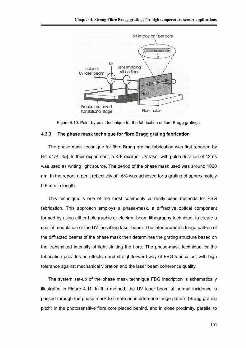
Chapter 4. Strong Fibre Bragg gratings for high temperature sensor applications
103
Figure 4.10: Point-by-point technique for the fabrication of fibre Bragg gratings.
4.3.3 The phase mask technique for fibre Bragg grating fabrication
The phase mask technique for fibre Bragg grating fabrication was first reported by
Hill et al. [45]. In their experiment, a KrF excimer UV laser with pulse duration of 12 ns
was used as writing light source. The period of the phase mask used was around 1060
nm. In the report, a peak reflectivity of 16% was achieved for a grating of approximately
0.9 mm in length.
This technique is one of the most commonly currently used methods for FBG
fabrication. This approach employs a phase-mask, a diffractive optical component
formed by using either holographic or electron-beam lithography technique, to create a
spatial modulation of the UV inscribing laser beam. The interferometric fringe pattern of
the diffracted beams of the phase mask then determines the grating structure based on
the transmitted intensity of light striking the fibre. The phase-mask technique for the
fabrication provides an effective and straightforward way of FBG fabrication, with high
tolerance against mechanical vibration and the laser beam coherence quality.
The system set-up of the phase mask technique FBG inscription is schematically
illustrated in Figure 4.11. In this method, the UV laser beam at normal incidence is
passed through the phase mask to create an interference fringe pattern (Bragg grating
pitch) in the photosensitive fibre core placed behind, and in close proximity, parallel to

Optical fibre high temperature sensors and their applications
104
the phase mask used. The interference of the plus and the minus first-order diffracted
beams photo-imprints a refractive index modulation in the optical fibre core and thus
results in the formation of the gratings. The period of the grating fringe () is one-half of
the period of the phase mask (pm/2) used. Hence the Bragg wavelength of the fibre
gratings written can be given by:
pmeffeffB nn 2 (4.11)
One major advantage of the phase mask technique over the two-beam
interferometer technique is that the wavelength of Bragg gratings, as given in Equation
4.11, is independent of the writing laser wavelength. Thus the Bragg wavelength of the
gratings can be easily tailored by using different periods of phase masks. Additionally,
since the photosensitive fibre is placed directly behind the phase-mask in the near field
of the diffractive (plus and minus first-order) beams, the sensitivity to mechanical
vibrations (optical beam path length is reduced) is minimised. The use of one optical
diffractive element reduces the complexity of the fabrication system and thus makes the
device inherently more stable for reproducing identical samples.
Figure 4.11: Schematic illustration of a phase mask FBG fabrication technique.
Phase mask
UV laser beam
Cylindrical lens
FBG Optical Fibre Diffracted beams
Zero order (<3% of throughout)
-1st order 1st order
Fringe Pattern

Chapter 4. Strong Fibre Bragg gratings for high temperature sensor applications
105
In the work described in this thesis, this phase mask fabrication approach has been
used for all Bragg grating fabrication. The experimental setup used at City University for
the fabrication of fibre Bragg gratings is shown in Figure 4.12 schematically and Figure
4.13 photo graphically. A plano-cylindrical lens (focal length of 20 mm) is deployed to
converge the UV laser beam into a line (rectangular shape, beam length of around 6.5
mm) along the core of the photosensitive fibre. The KrF excimer laser beam is passed
through a uniform phase mask at normal incidence to create an interference pattern in
the photosensitive fibre core. The photosensitive fibre is placed just behind and in close
proximity, parallel to the phase mask and photo-imprinting a refractive index modulation
Excimer Laser
(248nm)
Broadband
Source
UV Beam
Cylindrical
Lens
Photosensitive
fibre
Phase Mask
Optical Spectrum
Analyser
Figure 4.12: Schematic of the experimental set-up for fabrication of fibre Bragg gratings using
the phase-mask technique at City University London.
Figure 4.13: FBG fabrication system at City University
Cylindrical lens
Phase mask and holder
Fibre holder

Optical fibre high temperature sensors and their applications
106
in the fibre core forms a Bragg grating. The fibre is connected to a broadband light
source and to an optical spectrum analyser (OSA) to monitor the spectral profile of the
grating formed during fabrication.
4.4 Strong Fibre Bragg gratings for high temperature applications
4.4.1 Commercial photosensitive fibres
As mentioned in the previous sections, the gratings written into a silica fibre are
mainly inscribed by exposing the fibre to interference pattern fringes created by a UV
laser beam from a KrF excimer laser working at 248 nm or a double frequency Argon
ion laser working at 244 nm, through a phase mask. With most of fibres, such as silica
fibres used for telecommunications, the photo-induced refractive index change is
negligible. While with some special fibres, the refractive index change is significantly
observable, and may result in a strong peak wavelength reflection, Bragg reflection.
This characteristics of the photo-induced reflective index change (permanently) in fibres,
when they are exposed to UV laser emission, is normally termed as photosensitivity,
and the fibres with high photosensitivity are termed as photosensitive fibres.
Since the discovery of the photosensitivity phenomena in silicas fibre in 1978 [6,7]
and the invention of external side-writing FBG fabrication technique in 1989 [8],
intensive research on photosensitive fibre has been undertaken. It was reported that
heavily germanium doped silica fibres are generally of highly photosensitive, and the
common telecommunication silica fibres, which of lower Ge concentration (namely less
than 4 mol%), are normally not photosensitive. The highly germanium doped silicate
fibre is the first fibre in which the photosensitivity phenomenon was observed [6].
Nowadays, widely commercially available high Ge doped fibres, such as those
fabricated by FibreCore limited, USA, normally have a germanium concentration of
about 20 mol%. These types of fibres are highly photosensitive when exposed to the UV
laser emission such as of 244 nm, 248nm and 193 nm. A value of 2.5 x 10⁻⁴ in the
refractive index change can be easily achieved when the fibre is exposed to UV laser
beam irradiative.

Chapter 4. Strong Fibre Bragg gratings for high temperature sensor applications
107
In additional to the highly Ge doped fibres, another commonly available commercial
photosensitive fibre is boron (B) doped germannosilicate fibre. Compared to the high Ge
fibres, the B/Ge co-doped fibre has shown a higher photosensitivity and a relatively
lower value of numerical aperture (NA), which means it is possible to keep a large core
diameter while retaining single mode characteristics. Since this type of B/Ge co-doped
fibres has very high photosensitivity, a large refractive index change of about 7.5 x 10⁻⁴
can be easily obtained after the fibre is exposed to a modest power of 1 W/cm2 from a
double frequency argon ion laser for several minutes [49]. The B/Ge co-doped fibre is
the “standard” type of photosensitive fibres used in this work.
4.4.2 Photosensitive fibres for high temperature FBG writing
The weak point of the fibre sensors based on FBGs written into conventional
photosensitive fibres, such as the commercially available Ge doped fibre and B/Ge
co-doped fibre, is their comparatively low temperature resistance. Normally, FBGs
written into B/Ge co-doped fibres decay rapidly at elevated temperatures and can be
completely washed out at temperatures over 350C within a few hours [50]. Because
of this irreversible degradation at high temperatures, the sensors based on FBGs
written into B/Ge co-doped fibre have their limitation in some applications, especially in
high temperature operation, although the silica fibre itself can survive temperatures over
1000oC for long term operations. The low temperature sustainability of these gratings is
mainly due to the decay of the photo induced refractive index change formed in the fibre
core during inscribing of the grating by the UV radiation.
Compared to FBGs written into B/Ge co-doped fibres, the performance of FBGs
inscribed into highly Ge doped fibre silica fibres is more stable at elevated temperatures.
Normally, type I gratings written into these Ge doped fibres can survive at temperatures
below 650oC for many hours. For type IIA gratings, the temperature sustainability is
even higher [10]. Almost no degradation of gratings is observed when they are annealed
at temperature below 650oC. However, further annealing test on the gratings written into
the high Ge doped fibres has shown that the gratings (both type I and type IIA) decay
very quickly at temperatures over 700oC and eventually disappear completely after

Optical fibre high temperature sensors and their applications
108
being annealed at 750oC for a few hours [49]. However the FBGs inscribed into high Ge
doped fibres are generally suitable for sensing applications in the moderate temperature
region. In order to expand the FBG applications to higher temperature, novels fibres
with higher temperature sustainability are desired.
Improving the high temperature sustainability of gratings is one of the main topics of
optical sensor research, with an aim to widen the sensing range of FBG-based fibre
sensors. If the operational temperature of FBG-based sensors can be increased to over
1000oC, FBG sensors will be suitable for a number of applications, such as aero-engine
heat leakage measurement and combustion temperature studies, temperature
monitoring in the oil and gas industries, and furnace lining temperature measurement,
temperature monitoring of high-power microwave set-ups, etc.
In light of the above, a detailed investigation has been conducted by the research
group at City University London and it was found that the host fibre materials play an
important role in determining the FBG thermal sustainability. In this work a brief
summary is given below in terms of the thermal sustainability of FBGs written in a
number of host fibres, including tin doped fibre [52-53] and erbium co-doped fibre
[51,54], antimony doped fibre [55] and Indium doped fibre [56].
4.4.2.1 Sn doped photosensitive fibres
Tin (Sn) doped photosensitive fibre was first developed by Dong et al [52], at
Southampton University, UK, by co-doping Sn into the fibre core of phosphosilicate fibre
to increase its photosensitivity. It was found that with the presence of a small amount of
Sn in the core of the phosphosilicate fibre or germanosilicate fibre, an enhanced
photosensitivity of the fibre can be realized and strong gratings can be inscribed into
these fibres [53]. Further research by the City group reported that FBGs written into
the Sn doped fibre could survive at very high temperatures, over 800oC, and a
considerable value of reflectivity remained after annealing at such an elevated
temperature for several hours [52]. However the photosensitivity of this specialist fibre is
not as good as that of B/Ge fibres. To fabricate a FBG with a reflectivity of over 95% into
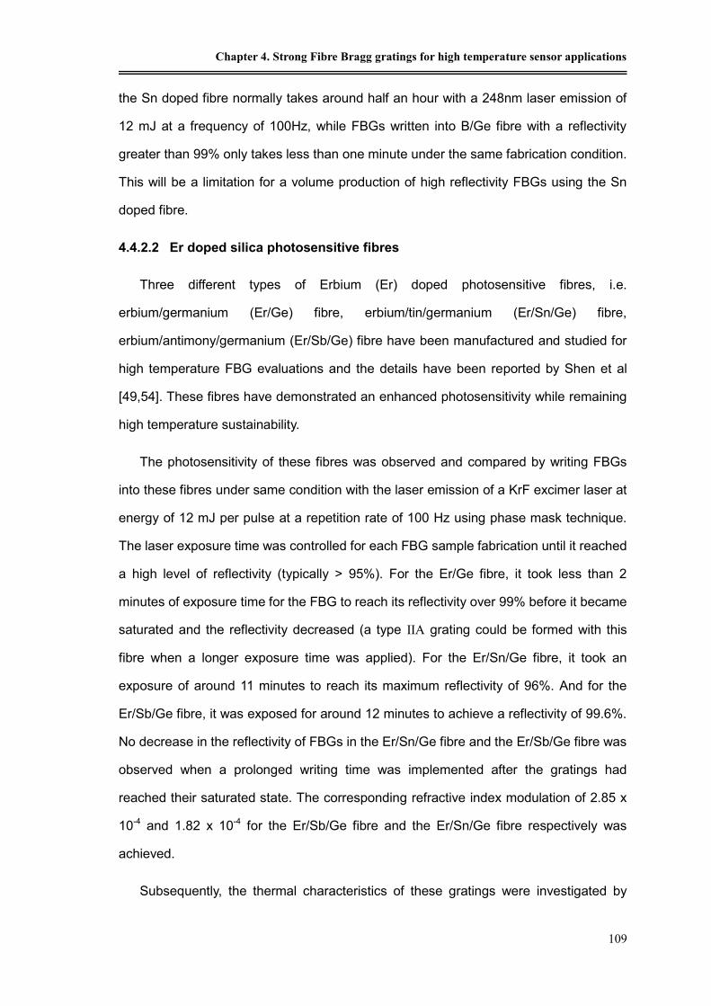
Chapter 4. Strong Fibre Bragg gratings for high temperature sensor applications
109
the Sn doped fibre normally takes around half an hour with a 248nm laser emission of
12 mJ at a frequency of 100Hz, while FBGs written into B/Ge fibre with a reflectivity
greater than 99% only takes less than one minute under the same fabrication condition.
This will be a limitation for a volume production of high reflectivity FBGs using the Sn
doped fibre.
4.4.2.2 Er doped silica photosensitive fibres
Three different types of Erbium (Er) doped photosensitive fibres, i.e.
erbium/germanium (Er/Ge) fibre, erbium/tin/germanium (Er/Sn/Ge) fibre,
erbium/antimony/germanium (Er/Sb/Ge) fibre have been manufactured and studied for
high temperature FBG evaluations and the details have been reported by Shen et al
[49,54]. These fibres have demonstrated an enhanced photosensitivity while remaining
high temperature sustainability.
The photosensitivity of these fibres was observed and compared by writing FBGs
into these fibres under same condition with the laser emission of a KrF excimer laser at
energy of 12 mJ per pulse at a repetition rate of 100 Hz using phase mask technique.
The laser exposure time was controlled for each FBG sample fabrication until it reached
a high level of reflectivity (typically > 95%). For the Er/Ge fibre, it took less than 2
minutes of exposure time for the FBG to reach its reflectivity over 99% before it became
saturated and the reflectivity decreased (a type IIA grating could be formed with this
fibre when a longer exposure time was applied). For the Er/Sn/Ge fibre, it took an
exposure of around 11 minutes to reach its maximum reflectivity of 96%. And for the
Er/Sb/Ge fibre, it was exposed for around 12 minutes to achieve a reflectivity of 99.6%.
No decrease in the reflectivity of FBGs in the Er/Sn/Ge fibre and the Er/Sb/Ge fibre was
observed when a prolonged writing time was implemented after the gratings had
reached their saturated state. The corresponding refractive index modulation of 2.85 x
10-4 and 1.82 x 10⁻⁴ for the Er/Sb/Ge fibre and the Er/Sn/Ge fibre respectively was
achieved.
Subsequently, the thermal characteristics of these gratings were investigated by

Optical fibre high temperature sensors and their applications
110
testing in a tube oven. The temperature of the oven was raised from room temperature
to around 900oC with steps of 100oC or 50oC each time, and at each temperature the
FBGs were annealed for 24 hours. The results obtained clearly indicated that the
grating written in the Er/Ge fibre was erased at 700oC, and those written in the Er/Sb/Ge
and Er/Sn/Ge fibres still retained a considerable level of reflectivity after being annealed
at 850oC for 24 hours and 900oC for 4 hours respectively. The results obtained are of
great importance for high temperature applications.
4.4.2.3 Sb/Ge co-doped fibre and In/Ge co-doped fibre
Based on the results obtained, Shen et al. have designed and fabricated more
photosensitive fibres in order to meet requirements for even higher temperature
applications. A novel Sb/Ge co-doped fibre has been specially designed and developed
for the fabrication of “strong” gratings with very high temperature sustainability. The fibre
is of high photosensitivity with FBGs inscribed into it can reach a high refractive index
modulation of greater than 2.7 x 10⁻⁴. The FBG written into the Sb/Ge co-doped fibre,
with initial reflectivity over 99%, could sustain an elevated temperature of 900oC over a
period of 24 hours and yet retained a considerable level of reflectivity of over 18%. It
remained a reflectivity of 3.4% after having been annealed at extreme high temperature
of 950oC over a period of 8 hours, with an observable reflection peak after 20 hours.
These results were much better than those obtained from Sn doped fibre [56] and
Sb/Er/Ge [57] co-doped fibres reported earlier.
In addition to the Sb doped fibre, Shen et al. also developed a Indium (In) co-doped
germanosilicate fibre for high temperature FBG inscribing with high photosensitivity[58].
The gratings can reach high reflectivity of 99.0% and 99.8% using the excimer laser of
12 mJ per pulse with repetition rates of 200 Hz and 300 Hz respectively, representing
refractive index modulation of 2.4 x 10⁻⁴ and 3.2 x 10⁻⁴. After having being annealed at
900oC for 24 hours, the gratings retained a considerable level of reflectivity of 11% (200
Hz repetition rate) and 21% (300 Hz repetition rate). After being annealed at 950 oC for
hours and 1000 °C for 2 hours before the annealing temperature was cooled down to
the room temperature step by step. The retained reflective spectrum showed that the

Chapter 4. Strong Fibre Bragg gratings for high temperature sensor applications
111
reflectivity of the grating could still be interrogated by instrumentation.
4.4.3 Strong FBGs written into Bi/Ge co-doped fibres
Further to the study of Sb doped and In doped fibre, which has shown that these
fibres had good photosensitivity and a strong temperature sustainability of the gratings
written into them, another type of high photosensitive fibre was specially developed,
with partners at Zhejiang University, China and the China Building Materials Academy,
for systematic evaluations of the gratings at high temperatures. The temperature
sustainability and thermal decay of the FBGs written into this fibre were observed and
evaluated.
4.4.3.1 Fabrication of Bi/Ge co-doped fibre
In an attempt to investigate a novel and highly photosensitive fibre for extreme high
temperature FBG applications, the bismuth doped germanosilicate fibre (Bi/Ge fibre),
was developed. The choice of the element bismuth was mainly made on the basis of the
electron charge effect of the outer shell electrons in the atom, similar to the situation in
In-doped fibre, with the large cation Bi3+ ion size (130 pm, greater than that of 76 pm of
Sb3+ and 80 pm of In3+) in its atomic construction [59]. It is believed that this larger size
of the doping ion may effectively stabilize the performance of the material concerned, as
in the situation of the fluorescence performance of Tm-doped Yttrium Aluminium Garnet
(YAG), where the doping of the Tm ion composition has created a garnet with a very
stable fluorescence intensity and decay lifetime when experiencing annealing
temperatures as high as 1200 oC [60]. The choice of doping another element, Ge, in the
fibre is aimed both to enhance the photosensitivity of the fibre and to increase the
refractive index of the fibre core.
The fibre was fabricated at the China Building Materials Academy, Beijing, China as
a joint research venture. The fibre preform, with a composition of GeO2 ~15 wt%,
Bi3+:5000 ppm, was fabricated by the method of Modified Chemical Vapour Deposition
(MCVD. A long length of fibre with a core diameter of about 8 µm and a cladding
diameter of 125 µm was then drawn from the preform at 2100 oC, using the normal fibre

Optical fibre high temperature sensors and their applications
112
drawing approach.
4.4.3.2 FBGs written into the Bi/Ge co-doped fibre
A number of strong FBG samples were fabricated into the specially developed
Bi/Ge fibre through phase mask technique, using ultra-violet (UV) exposure at a
wavelength of 248nm from a KrF excimer Laser with an energy of 10-12mJ per pulse at
a repetition frequency of 100Hz or 200hz. An optical spectrum analyzer (OSA) was used
to monitor the reflectivity of the grating during fabrication. The total exposure time was
from 5 minutes to 15 minutes for these FBGs. The increasing reflectivity of some of
these gratings with exposure time is illustrated in Figure 4.14. It is clearly shown that the
grating can easily reach a high reflectivity (greater than 99% for the samples used here)
in 5 to 15 minutes, varying with the writing condition. It takes a much longer time for
writing high reflective gratings compared to Ge doped fibre and B/Ge co-doped fibre,
which require around 1 minute laser exposure to reach the reflectivity over 99%.
4.4.4 Thermal characteristics of strong FBGs written into Bi/Ge fibre
The thermal characteristics of the strong FBGs written into the special
photosensitive fibre were tested at the laboratory of City University by annealing the
gratings in a tube oven at different temperatures. The experimental setup is illustrated in
Figure 4.15. The gratings were put into a tube oven and loosely placed at the centre of it.
The transmission spectrum of the FBG was monitored by an OSA (HP86140A), when
the grating was illuminated by light from an ASE broadband light source. The Bragg
wavelength and the reflectivity of the grating were recorded and analysed. Several
different annealing procedures were carried out, which are detailed as follows.

Chapter 4. Strong Fibre Bragg gratings for high temperature sensor applications
113
Exposure time (Minute)
0 2 4 6 8 10 12 14 16
Re
fle
ctivity (
%)
40
50
60
70
80
90
100
grating 1 (10mJ @100Hz)
grating 2 (10mJ @100Hz)
grating 3 (10mJ @200Hz)
grating 4 (12mJ @200Hz)
(In the bracket are the energy and frequency of the laser pulse)
Figure 4.14: Reflectivity change of FBGs vs. exposure time during fabrication
4.4.4.1 Thermal decay test of the FBGs
The thermal decay characteristics of FBG sample 1 were observed over the
temperature range from 300oC to 900oC, in increments of 100oC. The FBG was
Figure 4.15: Experimental set-up for testing the temperature characteristics
of the strong FBGs written into a Bi/Ge fibre
Single-mode optical fibre
OSA(HP86140A) Carbolite oven
800 C
FBG 12.4
ASE light source

Optical fibre high temperature sensors and their applications
114
annealed at each isothermal temperature for about 24 hours. The Bragg wavelength
shift and the reflectivity change of these FBGs are shown in Figure 4.16. It is clearly
shown that the FBGs, could sustain a high temperature of 900oC for 24 hours, and yet
still remained a considerable reflectivity of about 20%. The Bragg wavelength, as
expected, increased with any increase of temperature. Whereas, at each isothermal
temperature, a small wavelength shift towards a shorter wavelength was observed
along with the elapsed time, taking about 8-10 hours to reach an relative stable value of
B(T) at each temperature. This shift of B at each temperature of these FBGs is similar
to that of the FBGs written into some Ge doped and B/Ge co-doped fibres, which has
been discussed by Pal et al [61].
Annealing time (Hour)
0 20 40 60 80 100 120 140
Re
fle
ctivity (
%)
0
20
40
60
80
100
Wavele
ngth
(nm
)
1540
1542
1544
1546
1548
1550
1552
1554
400oC
500oC
600oC
700oC
800oC
900oC
300oC
Figure 4.16: The Bragg wavelength shift and reflectivity change of FBG, annealed
at temperatures from 300oC to 900
oC.
4.4.4.2 High temperature sustainability tests
A further annealing procedure was applied to three other FBG samples, gratings 2,
3 and 4, created in a similar way to grating 1. They were first annealed at 550oC for over
650 hours, then at 650oC for 190 hours and finally at 850oC for 55 hours. The decay of
the reflectivity and the wavelength shift of these gratings with the annealing time are
illustrated in Figure 4.17. The reflectivity of gratings 3, 4 and 5, after being annealed at
550oC for 650 hours, were 57%, 67% and 70% respectively, reduced to 37%, 46% and
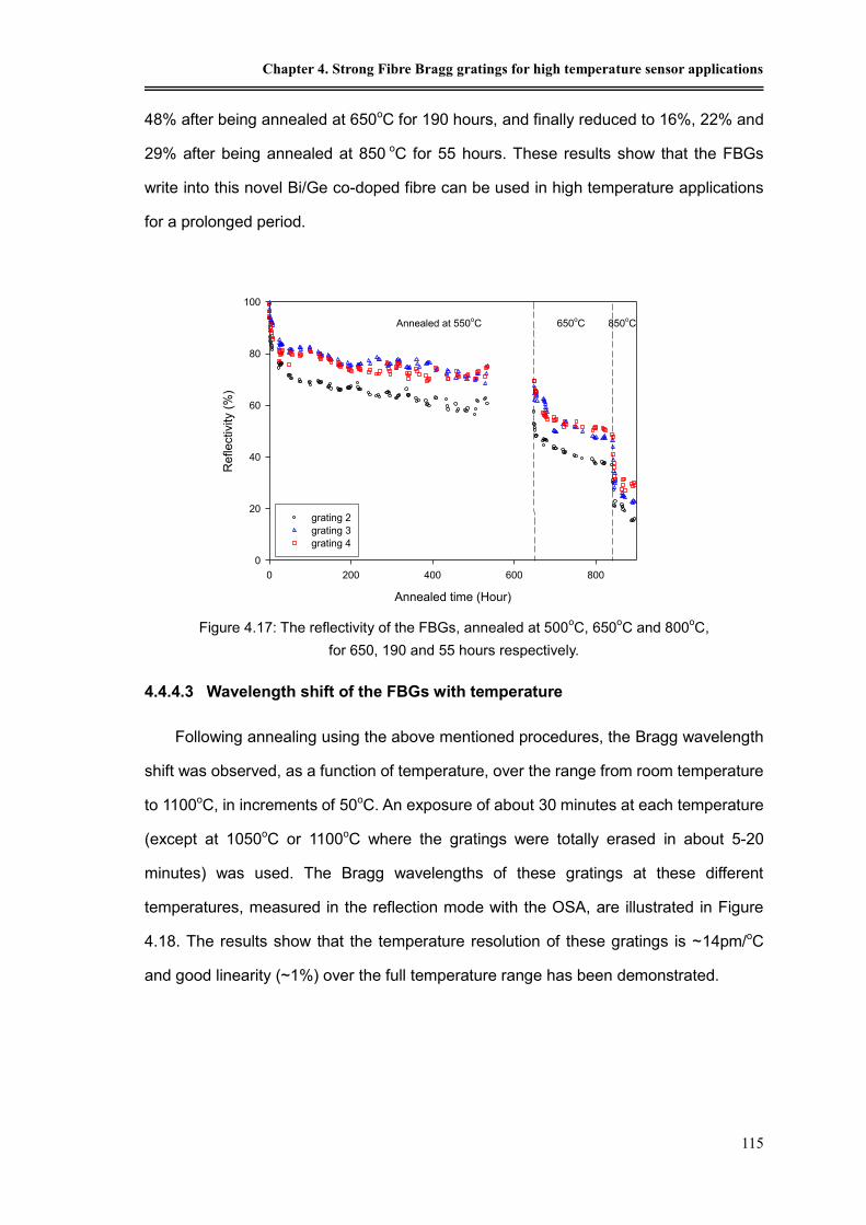
Chapter 4. Strong Fibre Bragg gratings for high temperature sensor applications
115
48% after being annealed at 650oC for 190 hours, and finally reduced to 16%, 22% and
29% after being annealed at 850 oC for 55 hours. These results show that the FBGs
write into this novel Bi/Ge co-doped fibre can be used in high temperature applications
for a prolonged period.
4.4.4.3 Wavelength shift of the FBGs with temperature
Following annealing using the above mentioned procedures, the Bragg wavelength
shift was observed, as a function of temperature, over the range from room temperature
to 1100oC, in increments of 50oC. An exposure of about 30 minutes at each temperature
(except at 1050oC or 1100oC where the gratings were totally erased in about 5-20
minutes) was used. The Bragg wavelengths of these gratings at these different
temperatures, measured in the reflection mode with the OSA, are illustrated in Figure
4.18. The results show that the temperature resolution of these gratings is ~14pm/oC
and good linearity (~1%) over the full temperature range has been demonstrated.
Annealed time (Hour)
0 200 400 600 800
Re
fle
ctivity (
%)
0
20
40
60
80
100
grating 2
grating 3
grating 4
Annealed at 550oC 650
oC 850
oC
Figure 4.17: The reflectivity of the FBGs, annealed at 500oC, 650
oC and 800
oC,
for 650, 190 and 55 hours respectively.

Optical fibre high temperature sensors and their applications
116
Temperature (oC)
0 200 400 600 800 1000 1200
Wa
ve
len
gth
(n
m)
1535
1540
1545
1550
1555
1560
1565
1570
grating 1
grating 2
grating 3
grating 4
Figure 4.18: The temperature dependent Bragg wavelengths of the FBGs, from room
temperature to 1100oC.
4.4.4.4 High temperature measurement – “shock test”
Some of the FBGs created with an initial reflectivity of >99%, without being
pre-annealed, were exposed to a high temperature for “shock” test. The FBGs, placed
loosely into a 1mm diameter stainless steel tube, were quickly inserted into the high
temperature zone in the oven, which was pre-set to a high temperature, typically
1000oC or 1100oC. A K-type thermocouple is intimately attached to the steel tube with
the FBG inside. The wavelength and reflected light intensity were recorded, using a
MicronOptics sm125 Optical Sensing Interrogator, until the FBGs were totally erased.
The results obtained, together with one set of data obtained from a FBG written into
B/Ge co-doped fibre for comparison, are shown in Figure 4.19. The tests show that the
FBGs written into the Bi/Ge fibre survived for ~15 seconds after being inserted in the
oven at 1100oC, and ~300 seconds at 1000oC. By contrast, the FBG written into B/Ge
fibre, when inserted into the oven at 1000oC, only lasted a few seconds before it was
completely erased as the temperature rose beyond 800oC. The results again clearly
indicate that the Bi/Ge FBG had much higher temperature sustainability, even when it
was exposed to a sudden high temperature change. However, these FBGs, which were

Chapter 4. Strong Fibre Bragg gratings for high temperature sensor applications
117
not pre-annealed, tended to last for a shorter time at high temperatures than those
which had been annealed, as the thermal pre-treatment is known to stabilise the index
modulation of the fibres [62].
Time (seconds)
1 10 100 1000
Re
fle
ctivity (
%)
0.0
0.2
0.4
0.6
0.8
1.0
Tem
pera
ture
(oC
)
0
200
400
600
800
1000
Bi-Ge fiber FBG at 1100oC
Bi-Ge fiber FBG at 1000oC
B-Ge fiber FBG at 1000oC
Figure 4.19: ‘Shock’ test of FBGs at 1000oC and 1100
oC
The experimental results from the tests on high temperature exposure and
annealing of the specialized FBGs created have clearly indicated that gratings inscribed
in the Bi/Ge fibre had much high temperature sustainability than those written into
conventional fibres. The results of this work give clear evidence that such gratings are
well suited to those sensing applications where high temperature sustainability is
essential.
In addition, the temperature sustainability of the FBGs created in the Bi/Ge fibre was
observed to be related to the initial reflectivity arising from the initial UV exposure of the
fibre during the grating writing. This observation suggests that an initial reflectivity
of >99% is preferred for high temperature applications.
4.5 Summary
After giving a brief review and introduction of fibre Bragg gratings and their
applications in telecommunications and sensors, the focus of the study has been on the

Optical fibre high temperature sensors and their applications
118
evaluation and cross-comparison of a number of gratings written into different host fibre
materials for their thermal sustainability for potential high temperature applications. The
photosensitivity and thermal characteristics of fibre Bragg gratings inscribed in a newly
developed Bi/Ge co-doped fibre have been systematically tested and evaluated. The
results show that the strong gratings written into the Bi/Ge fibre can retain high
reflectivity after being annealed at elevated temperatures over 900 oC, therefore are
well suitable for high temperature applications.
Reference
[1]. B. A. Childers, M. E. Froggatt, S. G. Allison, T. C. Moore, D. A. Hare, C. F. Batten
and D C. Jegley, “Use of 3000 Bragg grating strain sensors distributed on four 8-m
optical fibers during static load tests of a composite structure”, Proc. SPIE Vol. 4332,
Smart Structures and Materials, 2001, pp.133-142
[2]. A. Othonos, “Fibre Bragg gratings”, Review of Scientific Instrument, Vol. 68, 1997,
pp.4309-4341.
[3]. A. Othonos and K. Kalli, “Fiber Bragg Gratings: Fundamnetals and Applications in
Telecommunication and sensing”, Artech House, 1999
[4]. Y. J. Rao, “Recent Progress in Applications of In-Fibre Bragg Grating Sensors”, Optics
and Engineering, 31, (1999), pp.297-324.
[5]. A. D. Kersey, M.A. Davis, H.J. Patrick, M. LeBlanc, K.P. Koo, C.G. Askins, M.A.
Putnam, E.J. Friebele, “Fiber grating sensors”, Journal of lightwave technology, Vol.
15, 1997, pp.1442-1463
[6]. K.O. Hill, Y. Fujii, D. C. Johnson, B. S. Kawasaki, "Photosensitivity in optical fibre
waveguides: application to reflection fibre fabrication", Applied Physics Letters, Vol.
32, 1978, pp.647-649.
[7]. B. S. Kawasaki, K. O. Hill, D. C. Johnson, and Y. Fujii, “Narrow-band Bragg reflectors
in optical fibres”, Optics Letters, Vol.3, 1978, pp.66-68.
[8]. G. Meltz, W. W. Morey and W. H. Gkenn. "Formation of Bragg gratings in optical fibres
by a transverse holographic method". Optics Letters, Vol.14, 1989, pp. 823-825
[9]. J. L. Archanbault, L. Reekie, and P. J Rusell, “100% reflectivity Bragg reflector
produced in optical fibers by single excimer laser pulse”, Electronics Letters, Vol. 29,
1993, pp. 453-455
[10]. W.X. Xie, W.X. Xie, P. Niay, P. Bernage, M. Douay, J.F. Bayon, T. Georges, M.
Monerie, B. Poumellec, “Experimental evidence of two types of photorefractive effects
occurring during photo inscriptions of Bragg gratings written within Germanosilicate
fibres”, Optical communications, Vol. 104, 1993, pp. 185-195
[11]. L. Riant, and F. Haller, “Study of the photosensitivity at 193nm and comparison with
photosensitivity at 240nm influence of fibre tension: Type IIA aging”, IEEE Journal of
Lightwave Technology, Vol. 15, 1997, pp.185-195
[12]. K.O. Hill, F. Bilodeau, B. Malo, D.C. Johnson, “Birefringent photosensitivity in

Chapter 4. Strong Fibre Bragg gratings for high temperature sensor applications
119
monomode optical fiber: Application to external writing or rocking filters”, Electronics
Letters, Vol. 27, 1991, pp. 1548-1550
[13]. R. Kashyap, R. Wyatt, and P. F. McKee, “Wavelength flatten saturated erbium
amplifier using multiple side-tap Bragg gratings”, Electronics Letters, Vol. 29, 1993,
pp. 1025-1026
[14]. A. Othonos, X. Lee and D. P. Tsai, “Spectrally broadband Bragg grating mirror for and
erbium doped fibre laser”, Optical Engineering, Vol. 35, 1996, pp1088-1092
[15]. J. Chow, G.Town, B. Eggleton, M. Ibsen, K. Sugden, and I. Bennion,
“Multi-wavelength generation of an erbium doped fibre laser using in-fiber comb
filters”, IEEE photonics Technology letters, 1996, pp.60-62.
[16]. G. A. Ball, W. W. Morrey, and W. H, Glenn, “Study of monomode erbium fiber laser”,
IEEE photonics Technology letters, Vol. 3, 1991, pp.613-615
[17]. J. L. Zyskind, V. Mizrahi, D.J. DiGiovanni, J.W Sulhoff,,“Short single frequency
erbium doped fiber laser”, Electronics letters”, Vol. 28. 1992, pp.1385-1286
[18]. R. P. Davey, R.P.E. Fleming, K. Smith, R. Kashyap, J.R. Armitage, “Mode-lock erbium
fiber laser with wavelength selected by means of fiber Bragg grating reflector”,
Electronics letters, Vol. 27. 1991, pp.2087-2088
[19]. S. G. Grubb, T. Strasser, W. Y. Cheung, W. A. Reed, V. Mizrahi, T. Erdogan, P. J.
Lemaire, A. M. Vengsarkar, D. J. DiGiovanni, D. W. Peckham, and B. H. Rockney,
“High-power 1.48m cascaded Raman laser u germanosilicate fibers”, Proc. Optical
Amplifier and Their applications, Davow, Switzerland, Paper SaA4, 1994
[20]. C. R. Giles, “Lightwave applications of fiber Bragg gratings”, IEEE photonics
Technology letters, Vol 7, 1995, pp.980-982
[21]. V. Mizrahi, T. Erdogan, D.J. DiGiovanni, P.J. Lemaire, et al. “Four channel fire grating
demultiplexer”, Electronics letters, Vol. 30. 1994, pp.780-781
[22]. J. J. Pan and Y Shi, “Steep skirt fibre Bragg grating fabrication using a new apodised
phase mask”, Electronics letters, Vol. 33(22), 1997, pp. 1895-1896
[23]. H. G. Winful, “Pulse compression in optical fiber filters”, Applied physics letters, Vol.
46, 1985, pp.527-529
[24]. C. R. Giles, V. Mizrahi, T. Erdogan, “Polarization-independent phase conjugatin of
lightwave signals”, IEEE photonics Technology letters, Vol. 7, 1995, pp.126-128
[25]. K. O. Hill and G. Meltz, “Fiber Bragg grating technology”, Journal of lightwave
technology, Vol. 15, 1997, pp. 1263-1276
[26]. J.R. Dunphy, G. Meltz, F. Lamm, and W. Morey, “Multifunction, distributed optical fibre
sensor for composite cure and response monitoring”, society of Photo-optical
instrumentation Engineering, Fibre Optic Smart Structure and Skins III, Vol.1370,
1990, pp.116-118
[27]. Internet reference: ic.are.nasa.gov/ic/projects/photonics/os/healthsensors/health.html
[28]. D. R. Hjelme, “applications of Bragg grating sensors in the characterization of scaled
marine vehicle models”, Applied optics, Vol. 36 1997, pp. 328-336
[29]. S. T. Vobra, M. A Davis, A. Dandridge, et al, “Sixteen channel WDM fibre Bragg
grating dynamic strain sensing for composite panel slamming tests”, Proceedings of
the optical fibre sensor conference (OFS12), Williansburg, VA, USA, 1997, pp. 328
[30]. E. J, Ferribele, “Fiber Bragg grating strain sensor: Present and future applications in

Optical fibre high temperature sensors and their applications
120
smart structures”, Optics and Photonics, Vol. 9, 1998, pp33-37.
[31]. E. Joseph Friebele, "Fiber Bragg Grating Strain Sensors: Present and Future
Application in Smart Structures," Optics & Photonics News, Vol. 9(8), 1998, 33- ()
[32]. Yung Bin Lin, Chih Liang Pan, Yuan Hung Kuo, Kuo Chun Chang and Jenn Chuan
Chern, “Online monitoring of highway bridge construction using fiber Bragg grating
sensors”, Smart Material Structure, Vol. 14, 2005, pp.1075-1082
[33]. P. Moyo, “Development of fiber Bragg grating sensors for monitoring civil
infrastructure”, Engineering Structures Vol. 27, 2005, pp.1828-1834
[34]. Liang Ren, Hong-Nan Li, Jing Zhou, Dong-Sheng Li and Li Sun, “Health monitoring
system for offshore platform with fiber Bragg grating sensors”, Optical Engineering,
Vol. 45, 2006, 084401;
[35]. Y.J. Rao, B. Hurle, D.J. Webb, D.A. Jackson, L. Zhang, and I. Bennion, “In-situ
temperature monitoring in NMR machines with a prototype in-fibre Bragg grating
sensors system”, Proceedings of the optical fibre sensor conference (OFS12),
Williansburg, VA, USA, 1997, pp. 646-649
[36]. YJ Rao, DJ Webb, DA Jackson, L. Zhang, and I. Ben- nion, “In-fibre Bragg grating
temperature sensor system for medical applications”, IEEE Journal of Lightwave
Technology, Vol. 15, 1997, pp. 779-785
[37]. E. Samset, T. Mala, R. Ellingsen, I. Gladhaug, O. Søreide, E. Fosse, “Temperature
measurement in soft tissue using a distributed fiber Bragg grating sensor system".
Minimally Invasive Therapy and Allied Technologies, Vol. 10, 2001, pp. 89-93.
[38]. N E Fisher, J Surowiec, D J Webb, D A Jackson, L R Gavrilov, J W Hand, L Zhang and
I Bennion., “In-fibre Bragg gratings for ultrasonic medical applications”, Measurement
Science and Technology”, Vol. 8 ,1997, pp.1050-1054
[39]. B.M. Cowie, D.J. Webb, B. Tam, P. Slack, P.N. Brett, “Distributive Tactile Sensing using
Fibre Bragg Grating Sensors for Biomedical Applications”, The First International
Conference on Biomedical Robotics and Biomechatronics (BioRob 2006), 2006, pp.
312 - 317
[40]. A. F. Fernandez, A Gusarov, B Brichard, M Decréton, F Berghmans, P Mégret, and A
Delchambre, “Long-term radiation effects on fibre Bragg grating temperature sensors
in a low flux nuclear reactor” Measurement Science and Technology, Vol. 15 ,2004,
pp.1506-1511
[41]. P. M. Cavaleiro, F.M. Araujo, A.B.L. Ribeiro, “Metal-coated fibre Bragg grating sensor
for electric current metering”, Electronics Letters, Vol. 34, 1998, pp. 1133 -1135
[42]. Jianmin Gong, C. C. Chan, M. Zhang, W. Jin, J. M. K. MacAlpine, and Y. B. Liao “Fiber
Bragg grating current sensor using linear magnetic actuator”, Optical Engineering, Vol.
41, 2002, pp557;
[43]. K. Krebber, W. Habel, T. Gutmann and C. Schram, “Fiber Bragg grating sensors for
monitoring of wind turbine blades”, Proceedings of the optical fibre sensor conference
(OFS17), 2005, pp. 1036-1039
[44]. B. Malo, K.O.Hill, F. Bilodeau, D.C. Johnson, J. Albert,. “Point-by-point fabrication of
micro-Bragg grating in photosensitive fibre using single excimer pulse refractive index
modification techniques”, Electronics letters, Vol. 29, 1993, pp.1668-1669
[45]. K. O. Hill, B. Malo, F. Bilodeau, D.C. Johnson, J. Albert, "Bragg grating fabrication in

Chapter 4. Strong Fibre Bragg gratings for high temperature sensor applications
121
monomode photosensitive optical fibre by UV exposure through a phase mask”,
Applied Physics letters, Vol. 62, 1993, pp.1035-1037
[46]. R. kashyap, “Fiber Bragg gratings”, Academic Press, New York, 1999
[47]. R. Kashyap, J.R. Armitage, R. Wyatt, S.T. Davey, D.L. Williams, “All-fiber narrow band
reflecting grating at 1500 nm”, Electronics Letters, Vol. 26, 1990, pp. 730-732
[48]. H. G. Limberger, P.Y. Fonjallaz, P. Lambelet, C. Zimmer,, “Photosensitivity and self
organization in optical fibers and waveguides”, SPIE, Vol.2044, 1993, pp.272
[49]. D. L. Williams, B.J. Ainslie, J.R. Armitage, R. Kashyap, R. Campbell, “Enhanced UV
photosensitivity in boron codoped germanosilicate fibres”, Electronics Letters, Vol. 29,
1993, pp.45-47
[50]. S. R. Baker, H.N. Rourke, V. Baker, D. Goodchild, “Thermal decay of fibre Bragg
gratings written in boron and germanium codoped silica fibre,” IEEE Journal of
Lightwave Technology, Vol.15, 1997, pp.1470-1477
[51]. Y. Shen, S. Pal, J. Mandal, et al, “Investigation on the photosensitivity, temperature
sustainability and fluorescence characteristics of several Er-doped photosensitive
fibres”, Optics Communications, Vol. 237, 2004, pp.301-308
[52]. L. Dong, J.L. Cruz, J.A. Tucknott, L. Reekie, D.N. Payne, “Strong photosensitivity
gratings in tin-doped phosphosilicate optical fibres”, Optics Letters, Vol.20, 1995,
pp.1982-1984
[53]. L. Dong, J.L. Cruz, L. Reekie, M.G. Xu. “Enhanced photosensitivity in tin-codoped
germanosilicate optical fibres”, IEEE Photonics Technology Letters, Vol. 7, 1995,
pp.1048-1050
[54]. Y. Shen, T. Sun, K.T.V. Grattan and M. Sun, “Highly photosensitive Sb/Er/Ge codoped
silica fibre for fibre Bragg grating (FBG) writing with strong high-temperature
sustainability”, Optics Letters, Vol.28, 2003, pp.2025-2027
[55]. Y. Shen, J. He, T. Sun, K.T.V. Grattan, “High temperature sustainability of strong FBGs
written into Sb/Ge co-doped photosensitive fibre - decay mechanisms involved during
annealing”, Optics Letters, Vol.29, 2004, pp.554-556
[56]. Y. H. Shen, “Charaterization of optical fibre sensor systems for applications at high
temperatures”, Ph D thesis, City University, London, 2005
[57]. G. Brambilla, V. Pruneri and L. Reekie, “Photorefractive index gratings in SnO2:SiO2
optical fibres”, Applied Physics Letters., Vol.76, 2000, pp. 807-809
[58]. Y. Shen, J. Xia, T. Sun and K.T.V. Grattan, “Photosensitive Indium doped
germano-silica fibre for strong FBGs with high temperature sustainability”, IEEE
Photonic Techology Letters, vol. 16, 2004, pp. 1319-1321
[59]. A. M. James and M.P. Lord, Macmillan’s Chemical and Physical Data, The MacMillan
Press Ltd, 1992
[60]. Y. H. Shen, W. Zhao, T. Sun and K.T.V. Grattan, “Characterization of optical fbre
thermometer using Tm3+:YAG crystal, based on fluorescence lifetime approach”,
Sensors and Actuators: A. Physical, Vol. 109, 2003, pp. 53-59
[61]. S. Pal, J. Mandal, T. Sun, and K.T.V. Grattan “Anlysis of thermal decay and prediction
of operational lifetime for a type I boron-germanium codoped fiber Bragg grating”,
Apply Optics, Vol. 42(12), 2003, pp. 2188-2197
[62]. J. Rathje, et al. “Continuous anneal method for characterizing the thermal stability of

Optical fibre high temperature sensors and their applications
122
ultraviolet Bragg gratings”, Journal of Applied Physics, Vol. 82(2), 2000, pp.
1050-1055

Chapter 5. Development of fibre Bragg grating based sensor systems for different applications
123
Chapter 5. Development of fibre Bragg grating based
sensor systems for different applications
5.1 Wavelength interrogation schemes of FBG sensors
For the FBG sensor applications,, such as temperature and/or strain sensors, the
accurate measurement of the Bragg grating wavelength shift is critical to achieve good
sensor performance. The simplest and easiest method to measure the spectrum of an
FBG(s) is using a commercially available Optical Spectrum Analyser (OSA). This
method is very commonly used in laboratories for preliminary sensor tests and
evaluations. But the spectrometers are very expensive. A normal OSA with a
wavelength resolution of 0.01nm costs over £15K. Particularly, in cases where a high
wavelength resolution, e.g. a resolution of 1 pm, is required to resolve a small
temperature change of 0.1oC, or stain change of 1 , the price of such an OSA is even
higher. In addition, conventional OSAs are very large and bulky, which limits their field
applications, especially for in-situ measurements. The OSAs, though providing some
functions for integration into user applications based on newly developed mathematical
models, do not usually have the flexibility to be developed fully as a cost-effective
interrogation system with a user-friendly interface for particular applications. Thus, it is a
challenge to create a low cost and compact electro-optics unit to replace an OSA to
accurately measure the Bragg grating wavelength (or its shift) and as a result a
considerable amount of research has been on-going to find an effective solution to this.
The most common method for interrogation of wavelength shift of Bragg gratings is
to use a broadband illumination, where the bandwidth of the broadband light source
covers the grating wavelength shift range when it is exposed to a perturbation. The
narrowband reflected light at the Bragg wavelength from the grating is then
subsequently directed to the wavelength detection system. Although a wide variety of
techniques have been demonstrated for monitoring Bragg wavelength shifts in many
literatures for the last few decades since the grating sensor system has been developed,

Optical fibre high temperature sensors and their applications
124
only a limited number of schemes appear to have the potential for being realized as a
practical, cost-effective instrumentation system for real-world applications. The
schemes of the wavelength interrogation system, which might be suitable for practical
applications, are listed in Table 5.1 [1], and discussed in the following sections.
Table 5-1: Summary of FBG wavelength interrogation schemes
Edge filter Tunable filter Interferometric Tunable
laser
CCD-
Spectrometer
Range to resolution 102-10
3 10
3-10
4 10
3-10
4 10
3-10
5 10
3-10
4
Measurement speed High high High high high
Long term stability Good good Good good good
WDM compatibility Low high High high high
Potential cost Low medium Low high medium
5.1.1 Edge filter wavelength interrogation scheme
One simple approach based upon opto-electronics is to measure the wavelength
shift using the edge filter method. In this method, an edge filter, which has a linear
relationship between wavelength shifts and the resulting output intensity changes, is
utilized for Bragg wavelength shift interrogation when its cutoff is close to the signal
wavelength,. As shown in Figure 5.1, the operational principle behind this method is that
the Bragg wavelength shift induced by the measurand is obtained by measuring the
intensity change from the output of the edge filter. The influences of the light source
fluctuations and losses in the optical links can be removed by consideration of a
reference signal. The wavelength shift can be obtained by measuring the ratio of the
signal intensity IS and the reference intensity IR, given by [2]:
(5.1)
where A is the sensitivity of the filter.
A resolution of tens of had been achieved for strain measurement by this low cost
system. This method offers several advantages over the OSA system in terms of low
cost and ease of use. However, it also has some intrinsic disadvantages, such as the
lack of multiplexing capability and limited resolution.
oB
R
S AI
I

Chapter 5. Development of fibre Bragg grating based sensor systems for different applications
125
Figure 5.1: Example of bulk edge filter wavelength interrogation system
An improved all-fibre approach, exploiting a WDM fused-tapered fibre coupler, has
been demonstrated to overcome the limitation and complexity of alignment of bulky
optics components [3]. By taking the ratio between the difference and the sum of the two
outputs, P1 and P2, from the two arms of the WDM coupler, as shown in Figure 5.2, the
drift-compensated output can be obtained and used for the FBG wavelength-shift
detection. This scheme offers the features of all-fibre approach, i.e. being very compact,
very low power loss and low cost, making it an ideal interrogation approach for relatively
low-accuracy measurements (typically ~1% of full measurement scale).
Figure 5.2: All fibre wavelength interrogation system based on a fibre
fused-tapered WDM coupler
Broadband light
source
2 x 2 Coupler
Detection
electronics
Detector
Linear
edge filter
Fibre link
FBG
2 x 2 Coupler
o
Edge filter
FBG signal
Broadband light
source
2 x 2 Coupler
Detector
Fibre link
FBG
WDM fibre coupler
Detector
21
21
PP
PP
Output
P1/P
P2/P

Optical fibre high temperature sensors and their applications
126
5.1.2 Tunable filter wavelength interrogation scheme
One of the most successful and attractive wavelength interrogation approaches is to
use a scanning optical filter to retrieve the wavelength changes of the FBG(s). The
principle of the approach is illustrated in Figure 5.3, a narrowband tunable filter is
scanning through over the whole range of the wavelength spectrum of the grating (or
gratings), which is luminated by a broadband light source, and the spectrum is given by
the scanned signal intensity against the control signal of the tunable filter.
NarrowbandTunable filter
FBGsignal
Control Signal
Outp
ut S
ignal
Figure 5.3: Optical scanning filter wavelength interrogation scheme
The optical filters include the fibre Fabry-Perot tunable filter [4], acoustic-optic filter
[5] and tunable fibre Bragg grating based filter [6], etc. Sensor systems based on these
filters have been demonstrated and deployed. Some specific examples of the above
filters are briefly presented in the following sections.
5.1.2.1 Fibre Fabry-Perot tunable filter
The Fabry-Perot filter is an optical resonator discovered by Charles Fabry and Albert
Perot in 1987[7]. This device has been used successfully in sensor and measurement
applications. This type of filters transmit a narrow band of wavelengths and rejects
wavelengths outside of that band. The interesting feature of these filters used for FBG
sensor applications is their ability to "select" the peak wavelength of the grating when
the filter is tuned, mainly by accurately displacing separation of the interference mirrors
using a piezoelectric (PZT) element. The narrow and stable filtering band of FP filters
makes them ideal for FBG wavelength interrogation and many FBG sensor systems
utilizing the FP filters have been developed and deployed in various applications [4,
8-10]. F-P filters are characterised by Free Spectral Range (FSR), minimum resolvable

Chapter 5. Development of fibre Bragg grating based sensor systems for different applications
127
bandwidth and filter finesse. These figures of merit of a FP filter are the major
parameters considered when selecting an appropriate filter for specific sensor
applications. The scanning rate of a tunable FP filter should also be taken into account
when dynamic measurement is required.
Figure 5.4 schematically illustrates how a tunable FP filter is employed to interrogate
the wavelength shift of a single FBG, which can be set either in a tracking (close-loop)
or scanning mode. In the scanning mode, which the F-P filter is scanned through the
interested spectral range, and can be used to address more than one grating, while in
close-loop mode, which is locked to the FBG wavelength by the feedback control
system, it can only address one FBG wavelength. A resolution of ~ 1pm over an
operation range of around 100 nm of such a system can be readily achieved.
Figure 5.4: FBG wavelength shift demodulation system using tunable FP filter
A number of the sensors can be easily multiplexed by using optical switches, which
is a notable advantage of tunable filter based wavelength interrogation system. Figure
5.5 demonstrates a FBG wavelength demodulation system based on a tunable filter,
which allows for addressing several serial arrays with over 60 sensors [10]. The number
of sensors can be further increased by increasing the number of switches or having a
multi-input/output port tunable filter.
Broadband
Source
Tunable fibre
FP filter
FBG
Reflected
light
Feedback
system
Output
Dither
Signal

Optical fibre high temperature sensors and their applications
128
5.1.2.2 Acousto-optic tunable filter
The acousto-optic tunable filter (AOTF) is all solid-state, compact, electronically
tunable with no moving components, narrow band light filter. The main component of an
AOTF is the birefringent acousto-optic crystal, where the interaction between the
acoustic wave and optical radiation occurs. When a light wave travels in the anisotropic
crystal, it is diffracted by the acoustic wave through the acousto-optic effect [11-12].
Changes in the acoustic frequency alter the diffraction properties of the crystal, enabling
very rapid wavelength tuning in the order of microseconds, limited only by the acoustic
transit time across the crystal. The AOTF has a very large wavelength tuning range being
up to several micrometres. Thus this type of opto-electronic devices provides an
attractive solution to wavelength multiplexing of a large number of FBG arrays [5,13-16].
Small changes in wavelength of the AOTF are linear to the changes of the applied
RF frequency, which is a very convenient parameter to be measured allowing for
accurate measurement and long term stability. There are two principal modes of
operation contributing to the wavelength demodulation of the FBGs using the AOTF:
scanning mode and lock-in mode. In scanning mode, as shown in Figure 5.6 (a) [17],
the AOTF is tuned via a voltage controlled oscillator (VCO) over the whole wavelength
range of interest. This mode is very useful for multi-FBG measurement. In lock-in mode,
the system tracks the instantaneous wavelength change of a particular grating using a
Figure 5.5: Schematic diagram of multiplexed FBG sensor electro-optic system with 60 sensors
ELED
FP filter
To 5 channels
of 12 FBGs
Reflected
light
Peak
detector
Current
controller
1x4 Switch
1x2 Switch
Digital controller
(ramp, timing)
I/O port
bus to PC
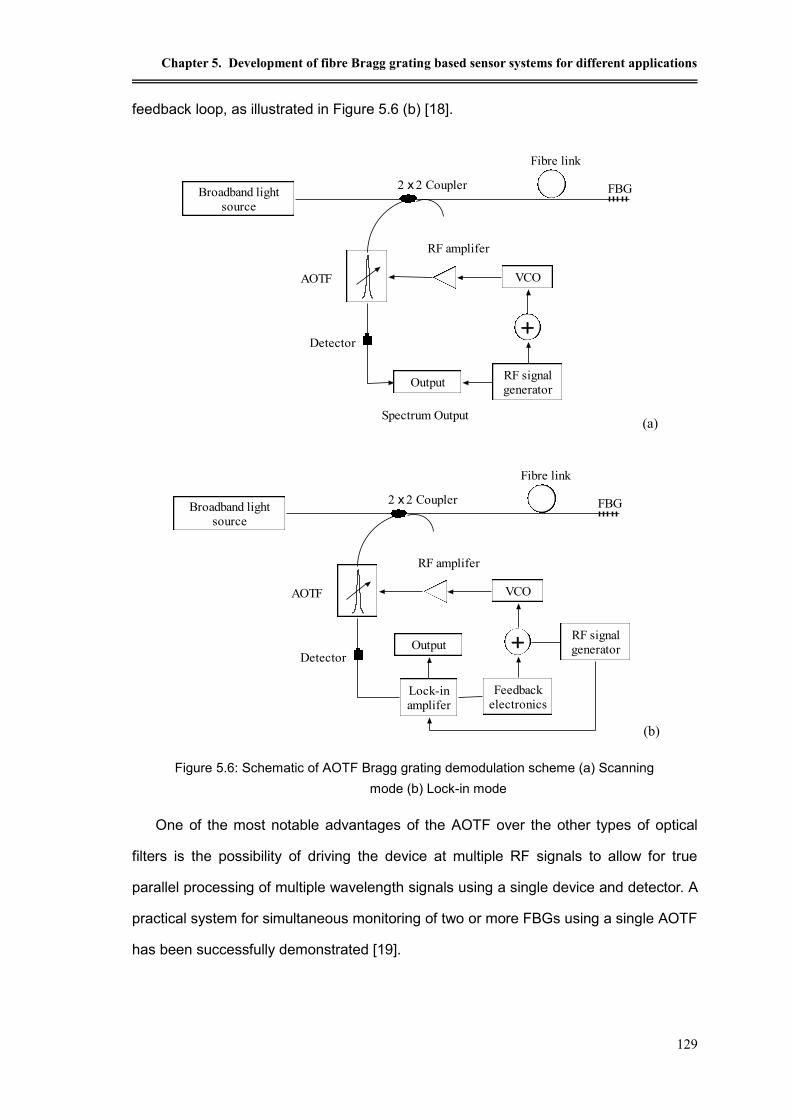
Chapter 5. Development of fibre Bragg grating based sensor systems for different applications
129
feedback loop, as illustrated in Figure 5.6 (b) [18].
(a)
(b)
Figure 5.6: Schematic of AOTF Bragg grating demodulation scheme (a) Scanning
mode (b) Lock-in mode
One of the most notable advantages of the AOTF over the other types of optical
filters is the possibility of driving the device at multiple RF signals to allow for true
parallel processing of multiple wavelength signals using a single device and detector. A
practical system for simultaneous monitoring of two or more FBGs using a single AOTF
has been successfully demonstrated [19].
Broadband light
source
2 x 2 Coupler
Detector
Fibre link
FBG
RF amplifer
Output
VCO
RF signal
generator
AOTF
Spectrum Output
Broadband light
source
2 x 2 Coupler
Detector
Fibre link
FBG
RF amplifer
Output
VCO
Lock-in
amplifer
Feedback
electronics
RF signal
generator
AOTF

Optical fibre high temperature sensors and their applications
130
5.1.2.3 Other tunable filters
Tunable fibre Bragg gating based filters have also been employed to track the
wavelength shift from FBG sensors [20-23]. With such a system, the measurement
range and resolution are mainly determined by the PZT element used in the system.
The system demonstrated by Brady et al. had measured strain and temperature with
resolutions of 2.8 and 0.2 oC, respectively. [20]
Coroy and Measures [24-25] have reported another type of wavelength
measurement systems, using a semiconductor quantum well electro-absorption filtering
detector (QWEFD). The system had a resolution of ±8 in strain and of ±9.7 pm in
wavelength
5.1.3 Tunable laser wavelength interrogation schemes
Calibrated, narrow-linewidth, single frequency, continuously wavelength-tunable
fibre lasers have been used to interrogate the wavelength shift of fibre grating sensors.
Different configurations of such fibre lasers have been employed for sensing
applications. Ball G. A. et al. [26] demonstrated an Er doped fibre laser source for
grating array interrogation. With an output power of 100mW in a 20 kHz linewidth, the
system achieved a temperature resolution of 0.18 oC over a temperature range from
room temperature to 180 oC. FBG sensor demodulation has also been implemented
using a broadband and short pulse generated mode-locked fibre laser [27-29]. The
system illustrated in Figure 5.7, has achieved a strain sensitivity of ±20 over a strain
range over 3500 , which is primarily limited by the total fibre dispersion.
In addition to the above mentioned tunable fibre laser source used for FBG
wavelength interrogation, other lasers have also been reported for FBG sensing
applications. Yun et al. have demonstrated a 0.1 nm linewidth, wavelength swept
erbium doped fibre laser, scanned over a 28 nm range and used to demodulate a FBG
array with a strain resolution of 0.47 at 250 Hz [30]. A supercontinuum light source
with 140 nm bandwidth pumped by a mode locked semiconductor laser source has also
been demonstrated for potential application in FBG sensors [31].

Chapter 5. Development of fibre Bragg grating based sensor systems for different applications
131
In general, FBG sensor systems interrogated using fibre lasers offer some
advantages over the other interrogation schemes, such as high resolution, high signal
noise ratio (SNR), and showing promise for long distance monitoring.
5.1.4 CCD spectrometer wavelength interrogation scheme
A fibre Bragg grating wavelength Interrogation scheme using a charge coupled
device (CCD) has also been implemented by some researchers for sensor applications
[32-34]. This method, as shown in Figure 5.8, can overcome the drawback of scanning
filters requiring sufficient overall optical power, but uses a parallel detection allowing all
reflected light to be detected by a CCD array. Since it collects all the light reflected by
the fibre gratings over the whole scanned range, ED = ER, and a grating even with 1%
reflectivity can provide as much signal required through this parallel detection, as a 95%
grating does via a scanned detection approach. The wavelength resolution of this
approach is determined by the linear dispersion of the grating at the detector plane per
pixel width, defined as nanometres per pixel (nm/pixel). The resolution can be further
improved by the so-called centroid detection algorithm[35], as the spectrum from each
(a)
(b)
Figure 5.7: (a) Passively mode-locked fibre laser source, using Er/Yb co-doped fibre
amplifier and dispersion compensating fibre. (b) Fibre Bragg grating array interrogation
system.
FBG array
EYDFA
DCF
PC
To array
diagnostics
Isolator
From
MLFL
Isolator
Coupler
DCF
To source
diagnostics
PC
To FBG
array
Coupler
PBS

Optical fibre high temperature sensors and their applications
132
grating is spread across many adjacent pixels, and a weighted average of the centre
wavelengths of the illuminated pixels scaled according to the incident signal level gives
a computed central grating wavelength. This and some other software algorithms can
dramatically improve the wavelength resolution and make it a very attractive approach
for many applications.
Figure 5.8: Schematic setup of fibre Bragg grating interrogation system employing a CCD-based
spectrometer [32]
5.1.5 Other wavelength interrogation schemes
Other fibre Bragg grating wavelength interrogation schemes, such as
Interferometric wavelength-shift detection [36-39] and Fourier transform spectroscopy
[40-42], have also been reported and demonstrated for different applications.
5.2 FBG-based temperature sensor using fibre Fabry-Perot tunable filter
With an overall consideration in terms of system performance, cost and flexibility in
multiplexing multiple FBG-based sensors is taken into account, a system using a
tunable fibre Fabry-Perot (FP) filter for FBG wavelength interrogation, may be
considered to be the most promising. This approach has shown to be able to satisfy
most of the application requirements and in this work such a system was specifically
built, tested, evaluated and discussed.
FBG arrays
Source
Collimator
Lens
Grating
CCD
array
Imaging
spectrograph
Images of fibre
from 1 to N
Images of fibre
from 1 to N

Chapter 5. Development of fibre Bragg grating based sensor systems for different applications
133
5.2.1 System setup
Figure 5.9 illustrates the operational principle of a FBG-based sensor system based
on Fabry-Perot tunable filter. The system mainly consists of four parts: (1) a broadband
light source, which can normally be a SLED or ASE source; (2) a FBG probe for
temperature and/or strain measurement, which contains one or more gratings; (3) a
wavelength interrogation system using a tunable F-P filter; (4) Interface software for
controlling, signal processing and data management.
BroadBand
Light Source
F-P tunable
filter
Electronics
DAQ Card
Wavelength Scan
Data Acquisition
FBG (T,)
2 x 2 coupler
Probe
Wavelength
detection systemDetector
FBG spectrum
Interface Software
Figure 5.9: Schematic system setup of a F-P filter based FBG sensor system
In the system, light from the broadband source, a SLED (DL5037 from Denselight
ltd, Singapore) with a central wavelength of 1550 nm and a bandwidth of 60 nm (HWFM)
and 3 mW output power in this case, is launched to the FBG probe through a 2 x 2
coupler, the reflected narrowband light at the Bragg wavelength, B, from the probe is
then launched into the tunable F-P filter (FFP-TF2 1580-003G4000-40 from
Micronoptics, USA), which scans through the wavelength range of interest under the
control signal, VF-P, from a DAQ card D/A output. The filtered optical signal through the
F-P filter is detected by an InGaSn PIN photo-detector and then is digitalized through
data acquisition with the DAQ card. The spectral profile, (), of the FBG probe can
thus be obtained from the digitized optical signal, IFBG, against the control scanning
signal, VF-P, following the equation below:

Optical fibre high temperature sensors and their applications
134
(5.2)
The Bragg wavelength, b, can be derived from the peak position, of the
spectrum, (), as:
(5.3)
and the above function can be pre-calibrated based on the data sheet of the
F-P filter provided.
In practice, the calibration of the wavelength against the corresponding scanning
signal is critical for the determination of the sensor system performance by using the
F-P filter approach. Generally, the wavelength spectrum can be calculated by the
following equation as a function of the control scanning signal, VF-P:
(5.5)
Normally, only a relative wavelength can be derived from equation 5.5. In order to
obtain the absolute wavelength of the FBG of the probe under a perturbation, a known
certain wavelength, ref, should be introduced as a wavelength reference. Thus the
wavelength can be obtained, based on the presumption that the performance of F-P is
linear over the wavelength range of interest, as shown in equation 5.3.
(5.6)
where is the corresponding scanning voltage of the F-P filter at a wavelength of
ref, and A is the scale of free spectrum range (FSR) and is the scanning voltage
over one FSR. If the non-linearity of F-P is taken into account, a more sophisticated
calibration process should be included.
Obviously, FBGs, one or two, or even more FBGs, at certain wavelengths can serve
as wavelength references for the F-P filter. This method offers a simple solution. To
),()( PFFBG VI
peak
PFV
0PF
FBG
V
IPF
peak
PFb VfVf
PFVf
)( PFVf
)()( ref
PFPFrefPF VVAVf
ref
PFV
PFV

Chapter 5. Development of fibre Bragg grating based sensor systems for different applications
135
achieve better performance with higher accuracy for wavelength measurement, some
other wavelength reference methods, such as using a traceable gas cell absorption
wavelength reference, might be used. The details of the FBG sensor systems based
on these wavelength reference methods will be discussed in the following sections.
5.2.1.1 F-P filter interrogation system with two FBGs as wavelength references
As mentioned above, FBGs with certain known wavelengths offer a convenient
solution to wavelength references for the F-P filter. If one FBG is used as a reference,
the measured wavelength can be obtained from equation 5.6. In a preliminary test of a
sensor system using one FBG as a reference, it was found that A in equation 5.6 would
change slightly with the operational time, especially in the early hours after the system
had started running. This resulted in a significant shift of the measured FBG
wavelength although the FBG was actually kept at a constant wavelength. The drift of
A is mainly caused by the intrinsic nature of the PZT used in the F-P filter to tune the
distance of the two fibre reflectors to achieve the interference.
In order to overcome this limitation, a sensor system with two FBGs as references
was then built. As illustrated in Figure 5.10, the light from a SLED is launched to a FBG
probe and two reference FBGs, which are connected respectively to the two ends of a
2x2 coupler. The reflected light which contains spectra from both of the probe and the
references is then passed through the coupler to the wavelength interrogation unit. A
typical spectrum is shown in Figure 5.11 where the wavelengths of the reference FBGs
with one being around 1528 nm and the other around 1570 nm, are located at the two
ends of the wavelength range of interest to be measured.

Optical fibre high temperature sensors and their applications
136
Figure 5.10: F-P filter interrogation system with two FBGs as wavelength reference
Figure 5.11: Spectrum obtained from both the FBG probe and two FBG references
As illustrated in Figure 5.11, the Bragg wavelength of the probe and the other
reference wavelengths shown in the spectrum, can be derived from the following
equation,
(5.7)
where , , are the wavelengths of the probe, references 1 and 2.
, , represent their corresponding scanning voltages of the F-P filter.
Compare to equation 5.6, the scale A in equation 5.6 is replaced by the term
SLED
F-P tunable
filter
Photo
Detector
Amplifier
ADWin
DSP Card
Wavelength Scan
Data Acquisition
PC
c: 1550nm
BW:~60nm
FBG (T)
2 x 2 coupler
FBGref1 FBGref2
Reference FBGs
BroadBand Light Source
Probe
Wavelength
detection system
Interface Software
VF-P
(V)
24 26 28 30 32 34 36
Inte
nsity (
V)
0.0
0.5
1.0
1.5
2.0
2.5
Wavelength (nm)
1520 1530 1540 1550 1560 1570 1580
ref1 probe ref2
Vref1
Vprobe
Vref2
1
12
12
1
ref
PF
probe
PFref
PF
ref
PF
refref
refprobe VVVV
probe 1ref 2ref
probe
PFV
1ref
PFV
2ref
PFV

Chapter 5. Development of fibre Bragg grating based sensor systems for different applications
137
in equation 5.7, which can be dynamically calculated during operation, in
order to eliminate the drift problem arising from the scale A. Figure 5.12 shows the
measured wavelength drift of two FBGs reference system within 15 hours after the
system being switched on, for comparison with that from the one FBG reference system.
During the test, the probe was kept at a constant temperature of 25oC with no strain
variation and the wavelength of the grating was expected to be stabilized at a certain
value. However, the measured wavelengths show a drift of around 80pm for the 2
reference FBGs system and 180 pm for the 1 reference FBG system, which represents
equivalent temperature changes of ~8 oC and ~18 oC respectively.
Figure 5.12: Measured wavelength drift within 15 hours of the F-P based sensor system with
FBGs as references
The above observed wavelength measurement drifts were mainly caused by two
effects. Firstly, the reference FBGs may have experienced a certain level of temperature
change during the measurement period. It has been observed that the temperature of
the system enclosure, where the reference grating was located, increased a few
degrees during the experiment. Secondly, the slight nonlinearity of the F-P filter
esulted in the wavelength calibration errors. This is especially evident for the one
12
12
ref
PF
ref
PF
refref
VV
Elapsed Time (hour)
0 2 4 6 8 10 12 14 16
Wavele
ngth
(nm
)
1535.50
1535.55
1535.60
1535.65
1535.70
1535.75
With 2 FBGs reference
With 1 FBG reference
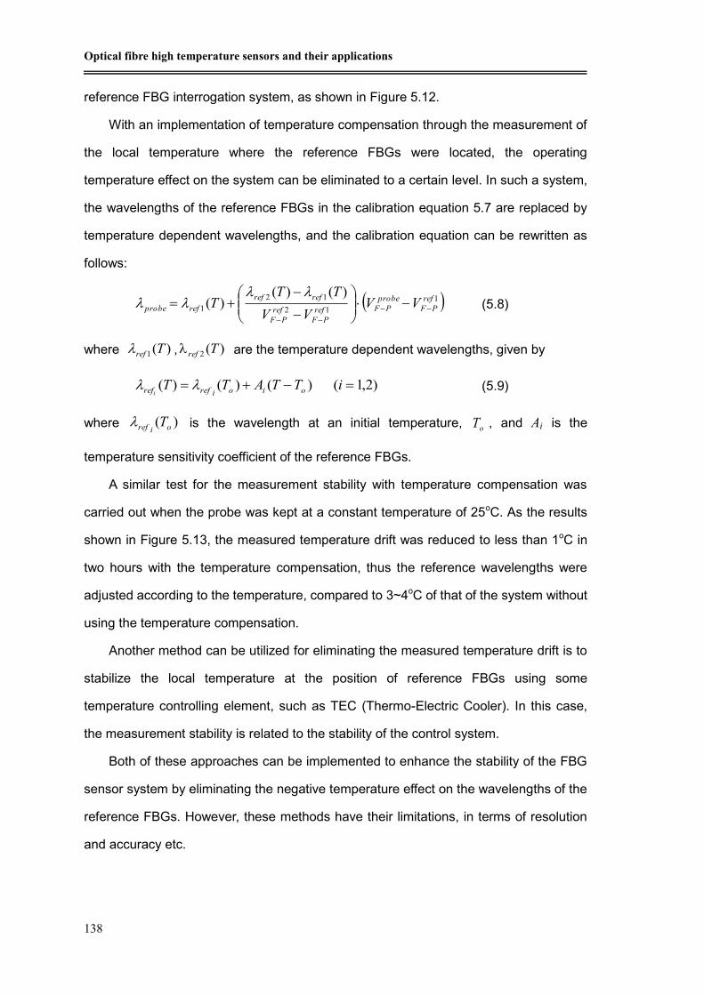
Optical fibre high temperature sensors and their applications
138
reference FBG interrogation system, as shown in Figure 5.12.
With an implementation of temperature compensation through the measurement of
the local temperature where the reference FBGs were located, the operating
temperature effect on the system can be eliminated to a certain level. In such a system,
the wavelengths of the reference FBGs in the calibration equation 5.7 are replaced by
temperature dependent wavelengths, and the calibration equation can be rewritten as
follows:
(5.8)
where , are the temperature dependent wavelengths, given by
(5.9)
where is the wavelength at an initial temperature, , and Ai is the
temperature sensitivity coefficient of the reference FBGs.
A similar test for the measurement stability with temperature compensation was
carried out when the probe was kept at a constant temperature of 25oC. As the results
shown in Figure 5.13, the measured temperature drift was reduced to less than 1oC in
two hours with the temperature compensation, thus the reference wavelengths were
adjusted according to the temperature, compared to 3~4oC of that of the system without
using the temperature compensation.
Another method can be utilized for eliminating the measured temperature drift is to
stabilize the local temperature at the position of reference FBGs using some
temperature controlling element, such as TEC (Thermo-Electric Cooler). In this case,
the measurement stability is related to the stability of the control system.
Both of these approaches can be implemented to enhance the stability of the FBG
sensor system by eliminating the negative temperature effect on the wavelengths of the
reference FBGs. However, these methods have their limitations, in terms of resolution
and accuracy etc.
1
12
12
1
)()()( ref
PF
probe
PFref
PF
ref
PF
refref
refprobe VVVV
TTT
)(1 Tref )(2 Tref
)2,1()()()( iTTATT oioirefrefi
)( oiref ToT

Chapter 5. Development of fibre Bragg grating based sensor systems for different applications
139
Figure 5.13: Temperature measurement drifts during operation of the FBG sensor system with
two reference FBGs, with and without temperature compensation
For the temperature compensation method, the inclusion of extra temperature
sensor(s), enables the resolution, accuracy and stability of that sensor to be carried
forward to affect the overall performance of the FBG senor system and this would
normally degrade the performance. The final temperature measurement accuracy of the
sensor will be given by:
(5.10)
where is the temperature measurement accuracy according to the grating
wavelength, and is the accuracy of the temperature sensor used for the
temperature compensation.
To fully optimize the performance of the FBG-based sensor system, some types of
operational temperature independent wavelength references (or wavelength calibration)
must be included. Therefore, in this work a FBG interrogation system with traceable gas
cell absorption as wavelength reference was built and evaluated, and will be discussed
in detail in the following section.
Time (minutes)
0 20 40 60 80 100 120 140 160
Tem
pera
ture
(oC
)
21
22
23
24
25
26
Without temperature compensation
With temperature compensation
koncompensati
AccuracyAccuracy
System
Accuracy TTT FBG
FBG
AccuracyT
koncompensati
AccuracyT

Optical fibre high temperature sensors and their applications
140
5.2.1.2 F-P filter FBG interrogation system with traceable gas cell absorption
reference
Traceable gas cells are able to use molecular absorption to provide standard NIST
(National Institute of Standards & Technology, US) traceable wavelength references
with unmatched stability over time irrespective of environmental disturbance. They are
commonly used as a standard for calibrating output signals of optical spectrum
analyzers. They have many other applications as well, for example as a wavelength
calibrator in many optical instruments, as a local reference for chemical sensing system,
for wavelength locking of lasers, spectroscopic research, and environmental and
physical sensing.
An F-P filter-based FBG wavelength interrogation system using a traceable gas cell
as a reference and a calibration standard for the wavelength correction is shown in
Figure 5.14. The broadband light scanned after the F-P filter is split into two using a 3
dB coupler. One branch of the coupler is connected to a gas cell, allowing the output
spectrum of the light to be measured based on the absorption lines of the gas cell. The
results obtained from the gas cell measurement are used for wavelength calibration of
the system. The other branch of the coupler is connected to FBG probes via a 2x2
fibre coupler. The reflected spectra of the probes can thus be obtained from the
calibration data obtained from the gas cell.
The traceable gas cell
The gas cell used in the system is hydrogen cyanide gas, HCN-13-C-100-FCPC,
supplied by Wavelength References, ltd, USA. It provides an equivalent standard of
the NIST SRM 2519, a standard wavelength calibration reference for 1530nm-1560nm.
The absorption spectrum of the gas cell is shown in Figure 5.14 and its main
specifications are listed in Table 5.2[43]. The gas cell provides very good wavelength

Chapter 5. Development of fibre Bragg grating based sensor systems for different applications
141
accuracy and temperature stability which is well suited for wavelength calibration in the
FBG sensor system. The wavelength shift is around 0.2pm when the operational
temperature changes 20oC. If there is no temperature compensation, this small
wavelength shift caused by the temperature variation can contribute to the system error
of the FBG interrogation system, although in most applications, this drift is considered to
be negligible.
Table 5-2: Specifications of the HCN gas cell
Wavelength Range nm 1525nm to 1565nm
Wavelength Accuracy pm ±0.3 (1 sigma, 100 Torr)
Temperature dependence pm <0.01/°C
Linewidth (-3dB) nm 0.070 typical (100Torr)
Wavelength calibration
As shown in Figure 5.15, the gas cell has a series of 51 absorption lines at discrete
wavelengths, (i= 1…51). The wavelength calibration of the system can thus be
obtained through the correlation between the measured absorption spectrum of the gas
cell and the F-P scanning voltage, which is related to the order of the data points taken
i
Abs
Figure 5.14: F-P filter based interrogation system with traceable gas cell reference
SLEDF-P tunable
filter
Photo
Detector
Amplifier
ADwin
DSP Card
Wavelength Scan
PC
c: 1550nm
BW:~60nm
1 x 2 coupler
BroadBand Light Source
Probe
Interface Software
Photo
Detector
Amplifier
Gas Cell
Wavelength Reference
Probe
2 x 2 coupler

Optical fibre high temperature sensors and their applications
142
through the DSP card sampling. The F-P control voltages, (i= 1…51),
corresponding to the absorption lines, can be derived from the absorption spectrum of
the gas cell, i(VF-P), using some peak (dip) searching algorithms. Then the wavelength
calibration equation can be obtained by data regression from the data set obtained
( ) ((i= 1…51). In practice, a 2nd order polynomial regression is used, and the
wavelength calibration equation is given by:
(5.11)
where A0, A1, A2 are the calibrated parameters, and VF-P is the control voltage of the F-P
filter in relation to the sampling data points.
In a practical system, the actual absorption spectrum obtained from the system,
shown in Figure 5.16, which is a absorption spectrum superimposed with the SLED light
source spectrum, may not be shown clearly to indicate the absorption lines as shown in
Figure 5.15. This is contributed by the use of a narrowband F-P filter, electronic noise
of the photo-detection system etc. As a result of this, some optimization techniques
are required to improve the system performance. The first step of such a technique is
to normalize the spectrum according to the light intensity at different wavelengths, and
i
PFV
i
PF
i
Abs V ,
2
210 )( PFPF VAVAA
Figure 5.15: Absorption spectrum of HCN gas cell

Chapter 5. Development of fibre Bragg grating based sensor systems for different applications
143
then reverse the signal to turn the absorption dips to numerical peaks for easy
algorithmic calculations, and furthermore this procedure allows initial peaks to be
selected (Figure 5.17a). The second step is to eliminate any unwanted peaks
appearing due to signal noises (Figure 5.17b). Finally it is important to recover those
peaks which were not detected as they were submerged in the noise (Figure 5.17c).
Figure 5.16: Actual gas cell absorption spectrum from the system
Data point (F-P voltage)
0 1000 2000 3000 4000 5000 6000 7000 8000 9000 10000
Inte
nsity (
Vo
lta
ge
)
3.0
3.5
4.0
4.5
5.0
5.5

Optical fibre high temperature sensors and their applications
144
(a)
(b) (c)
Figure 5.17: Optimization of the gas cell absorption for wavelength calibration through three
steps: (a) reversed gas cell absorption spectrum to detect initial peaks; (b) remove unwanted
peaked; (c) recover missing peaks
After the above optimization procedure, the wavelength calibration for the system
can be undertaken based on the optimized data set ( ) ((i= 1…51) using 2nd
order polynomial fitting as mentioned above. Figure 5.18 shows the results obtained
from a typical calibration process, which enables the wavelengths of the FBG sensors to
be calculated using the parameters obtained.
Wavelength (nm)
1510 1520 1530 1540 1550 1560 1570
Inte
nsity (
AU
)Reversed spectrum
Absorption peak
Missing peaks
unwanted peaks
1552 1553 1554 1555 1556 1557 1558
unwanted peaks
1560 1562 1564 1566
Missing peaks
i
PF
i
Abs V ,

Chapter 5. Development of fibre Bragg grating based sensor systems for different applications
145
Figure 5.18: Wavelength calibration of the gas cell absorption reference
Measurement stability and accuracy
It has been demonstrated that FBG wavelength interrogation system with a gas cell
reference had a very good stability and wavelength accuracy. Figure 5.19 shows the
temperature measurement in 2 hour using such a system, compared to that of the
system using 2-FBG reference. It is clearly shown that the gas cell based system had
Data point (F-P voltage)
2000 3000 4000 5000 6000 7000 8000
Wa
ve
leng
th (
nm
)
1525
1530
1535
1540
1545
1550
1555
1560
1565
Gas cell apsorption weavelength
Calibration data
Elapsed time (hour)
0.0 0.5 1.0 1.5 2.0
Te
mp
era
ture
(oC
)
20
22
24
26
28
30
With two-FBG reference
With gas cell wavelength reference
Figure 5.19: Cross-comparison of a FBG sensor system with gas cell reference and with two
grating reference

Optical fibre high temperature sensors and their applications
146
much better stability and accuracy of about ±0.1oC, while the accuracy of a 2-FBG
reference system was some ±1oC. Further evaluations of the system and results
obtained are presented in section 5.2.4.
5.2.2 Optoelectronic hardware of the system
The hardware setup of the system is shown in Figure 5.20. To make the prototype
a step closer to the commercial market, the system was designed in a modular format.
The system comprises four modules, and they are power supply module, light source
module, photo-detection and F-P control module, and DSP card. These modules are
interchangeable between different sensor units, thus making the system easier to be
debugged and/or repaired.
Power supply module
Two AC-DC modules, together with two DC-DC converter TMS 15512 and TMS
15124 from Traco Power Ltd, are used to provide quad outputs, +5 V, +24 V, and
±12 V. The 5V output is used for the DSP card and the SLED light source module.
24 V output is used for a bias voltage to enable the control of the F-P filter. The ±12
V outputs are used for the photo detection system.
Figure 5.20: Photo of the FBG based sensor system
(inset: the modular-based sensor interrogation unit )

Chapter 5. Development of fibre Bragg grating based sensor systems for different applications
147
Light source module
A thermally-cooled SLED, CS3705, from Denselight, Singapore, driven by a LD
current control module LD2332, from Wavelength Electronics, USA, is used to
provide a 3 mW broadband light with a 60nm 3dB bandwidth and a central
wavelength of 1555nm for the system. The operation temperature of the SLED is
controlled by a TEC for intensity stabilization.
Photo detection and F-P control module
Two channels of a 3-stage PIN photo-detector and amplifier are used to convert the
optical signals from FBGs and the gas cell when they are illuminated by a
broadband light into electrical signals. A signal conditioning circuit is also included
in this module to buffer the scanning signal from DSP card to control the F-P filter.
DSP card module
An ADwin-light-16-ERUO DSP card was specifically chosen and used in the system,
as it offers a cost-effective solution requiring only a limited number of inputs and
outputs. One analogue output is used for F-P filter scanning, and two analogue
inputs are used for FBG wavelength and gas cell absorption signal sampling. The
card has 8 analogue inputs, offering capacity for the upgrade to create a
multi-channel FBG sensor system.
5.2.3 Interface and control software
Interface software for the FBG based system has been programmed in LabView 7.1
platform. Figure 5.21 shows one screen printout of the main interface user panel.

Optical fibre high temperature sensors and their applications
148
Figure 5.21: Screen printout of the interface designed for FBG sensors
The main functions incorporated in the interface design have included:
F-P filter controlling
Data acquisition via the DSP card
Signal processing
Wavelength calibration
Temperature calibration
Data management
5.3 Test and evaluation of the FBG-based sensor system
5.3.1 Temperature calibration and resolution
Based on the specifications of the components used in the system, such as the
pass bandwidth of the F-P filter and the bandwidth of the FBG probe, the sensor system
should, theoretically, have an overall wavelength resolution of 1 pm, and a temperature
resolution of 0.1 oC. In this work, the system performance and the actual resolution of
the measurement was evaluated through a simple experiment set up for that purpose.
In order to verify the temperature resolution of the system, a standard setup which can
provide temperatures with a small step change (e.g. 0.1oC) should be used. However,
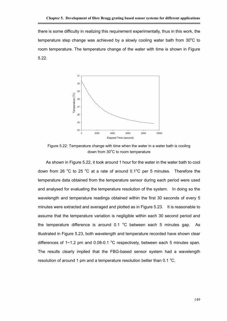
Chapter 5. Development of fibre Bragg grating based sensor systems for different applications
149
there is some difficulty in realizing this requirement experimentally, thus in this work, the
temperature step change was achieved by a slowly cooling water bath from 30oC to
room temperature. The temperature change of the water with time is shown in Figure
5.22.
Figure 5.22: Temperature change with time when the water in a water bath is cooling
down from 30oC to room temperature
As shown in Figure 5.22, it took around 1 hour for the water in the water bath to cool
down from 26 oC to 25 oC at a rate of around 0.1oC per 5 minutes. Therefore the
temperature data obtained from the temperature sensor during each period were used
and analysed for evaluating the temperature resolution of the system. In doing so the
wavelength and temperature readings obtained within the first 30 seconds of every 5
minutes were extracted and averaged and plotted as in Figure 5.23. It is reasonable to
assume that the temperature variation is negligible within each 30 second period and
the temperature difference is around 0.1 oC between each 5 minutes gap. As
illustrated in Figure 5.23, both wavelength and temperature recorded have shown clear
differences of 1~1.2 pm and 0.08-0.1 oC respectively, between each 5 minutes span.
The results clearly implied that the FBG-based sensor system had a wavelength
resolution of around 1 pm and a temperature resolution better than 0.1 oC.
Elapsed Time (second)
0 2000 4000 6000 8000 10000
Tem
pera
ture
(oC
)
24
25
26
27
28
29
30
31

Optical fibre high temperature sensors and their applications
150
Figure 5.23: Temperature and wavelength resolution of the FBG sensor system
5.3.2 Response time
The response time of system is determined by both the response time of the FBG
probe to temperature change and the scanning time of the wavelength interrogation
Time (second)
0 200 400 600 800
Te
mp
era
ture
(oC
)
24.8
25.0
25.2
25.4
25.6
25.8
26.0
26.2 FBG temperature reading
Average
Time (second)
0 200 400 600 800
Wa
vele
ng
th (
nm
)
1537.144
1537.146
1537.148
1537.150
1537.152
1537.154
1537.156
1537.158
1537.160
1537.162
1537.164
FBG wavelength reading
Average

Chapter 5. Development of fibre Bragg grating based sensor systems for different applications
151
system. The wavelength scanning time is mainly dependent on the scanning rate of the
F-P filter, which is up to 100Hz for the filter used. The actual scanning rate of the system
used was set at 10 Hz. The scanning rate could be increased but with a decreased
accuracy. Based on the experimental results obtained, the overall response time of the
sensor system was largely determined by the response time of the FBG to temperature
variation.
To investigate the response time of the FBG-based temperature sensor system, a
series of evaluation tests was carried out simply by dipping the probe into hot water at
temperatures of 90oC and 60oC respectively. The FBG probe was intimately attached to
a K-type thermocouple for cross comparison. Both temperature probes were exposed to
heated water baths at these temperatures for periods of 1 second, or 5 to 6 seconds.
The results of the tests are illustrated in Figure 5.24, which shows that the FBG system
can quickly respond to the temperature changes, both under the rising and falling
conditions. The thermocouple has also shown a rapid response to the temperature
Elapsed time (second)
0 20 40 60 80 100 120 140 160
Tem
pe
ratu
re (
oC
)
0
20
40
60
80
100Thermocouple
FBG
Exposed to 90oC for
1 Sec 1 Sec 5 Sec
Exposed to 60oC for
1 Sec 1 Sec 5 Sec
Figure 5.24: Temperature change while the FBG probe being dipped into and taking out form hot
water tank.

Optical fibre high temperature sensors and their applications
152
rising but could not reach the actual value within 1 second. It also had a slower
response to decreasing temperatures compared to that of the FBG probe. The results
clearly show that the FBG system has a faster response than that of the thermocouple.
Another experiment for evaluating the response time of the system was carried out
by testing the response of the FBG sensor to a temperature ‘spike’, rapid temperature
change. These ‘spikes’ were simulated by submerging the probe to the 90oC water
bath before and after being placed in a 60oC water bath. The FBG probe (together with
thermocouple), was dipped into the 90oC water bath (from room temperature) for
around 1 second, then was quickly removed from it within 1 second, before being
exposed to the 60oC water bath. Some sharp temperature changes (spikes) were
generated during this period. This procedure was repeated several times. The
temperature readings of the FBG system and the thermocouple were recorded, and as
shown in Figure 5.25 the temperature spikes were observed. The inset picture shows
the response of the temperature sensors to the first temperature ‘spike’ created. The
rapid temperature change was picked up by both the FBG probe and thermocouple,
however the fast temperature drop during the very short period (less than 1 second) by
moving the probes from 90oC water to air before being placed into the 60oC bath was
only detected by the FBG probe. This test showed that the FBG system could capture
a temperature spike when there was a rapid temperature change, and again, the
response time, which is less than 1 second, is quicker than that of the thermocouple.

Chapter 5. Development of fibre Bragg grating based sensor systems for different applications
153
Elapsed time (second)
0 100 200 300 400
Te
mp
era
ture
(oC
)
0
20
40
60
80
100
FBG
Thermocouple
60 62 64 66 68 70
0
20
40
60
80
100
Exposed to 90oC water for 1 second
before being moved to 60oC water
in 1 second
Exposed 90oC water for 1 second
before being moved from 60oC water
into air
Figure 5.25: Simulated temperature spike picked up by the FBG temperature sensor
5.3.3 Long term stability
The FBG-based system established was kept running continually for over 10 days
for long term stability test. The FBG probe, together with a K-type thermocouple, was
placed inside a tube oven for temperature monitoring. The oven was set at different
temperatures for testing the system stability at various temperatures. The results
obtained are shown in Figure 5.26, where a good long term stability of the FBG
temperature sensor system has been demonstrated during the test of 280 hours,
showing a comparable performance with that of the thermocouple. The slight
temperature discrepancy between the two sensors was attributed to the initial
calibration differences and their offset of locations .

Optical fibre high temperature sensors and their applications
154
Figure 5.26: Long term stability of the FBG-base sensor system, together with a
thermocouple, over 10 days
5.3.4 Absolute wavelength accuracy
As discussed above, both the wavelength resolution and relative wavelength
accuracy are important parameters for a FBG-based temperature sensor system, as the
wavelength shift is utilized for measurements. Absolute wavelength accuracy is
another important parameter for a sensor product.
In order to verify the absolute wavelength accuracy of the sensor system developed,
the absorption wavelengths of the traceable gas cell were measured by the FBG sensor
system (after some modifications of the software, as the original software was designed
specifically to detect FBG reflection peaks). Three HP18460 series OSAs were also
used in the laboratory for absorption peak search and identification. The wavelength
measurement deviations from the standards arising from the FBG system and OSAs
are shown in Figure 5.27. The results clearly indicate that the FBG system developed
has a higher absolute wavelength accuracy of around 10pm, compared to that of 150pm
for the OSAs.
Elapsed time (hour)
0 50 100 150 200 250 300
Tem
pe
ratu
re (
oC
)
0
100
200
300
400
500
FBG sensor
Thermocouple

Chapter 5. Development of fibre Bragg grating based sensor systems for different applications
155
Figure 5.27: Gas cell absorption wavelength (R Branch) measurement deviations arising from
the FBG system and OSAs
5.3.5 System performance specifications
Based on the extensive evaluation and calibration undertaken above, the system
specifications of the FBG based sensor system developed can be summarized in Table
5.3
Table 5-3: System specifications of the FBG based sensor system
Wavelength Accuracy (absolute) Better than 10 pm
Wavelength resolution 1 pm
Temperature resolution 0.1oC
Response time ~1 second
Gas cell wavelength (nm)
1526 1528 1530 1532 1534 1536 1538 1540 1542 1544
Mea
sure
men
t devia
tion (
pm
)
-200
-150
-100
-50
0
50
100
150
200
FBG system
OSA 1
OSA 2
OSA 3

Optical fibre high temperature sensors and their applications
156
5.4 Field tests of the FBG-based temperature sensor - Temperature monitoring
of automotive emissions
5.4.1 Background of the application
Exhaust emissions from cars, trucks and other road vehicles produce a major
source of air pollution [1]. The increasing traffic volume produces a high level of gas
species, such as CO, NOx, HC and SOx, in the urban environment, which affects the
health of human beings and animals. It has become vital to keep pollutant emissions to
a minimum. Using emission control technology is a practical way to do this, involving
reliable, robust and cost effective means of monitoring the pollutant and containment
levels in the exhaust systems.
The main pollutants, CO, NOx, HC and SOx, can be monitored through the
measurement of spectroscopic absorptions by specific pollutant gases in the vehicle
exhaust system. It is also important to measure the temperature of the exhaust gases,
as the optical absorption of the various species is temperature dependent, and for
control of the engine operational conditions.
Vehicle emissions can be hostile, with hot corrosive gases being present. In
addition, electromagnetic interference (EMI) in vehicles is a growing problem in sensor
design for the range of measurements required. For example, the use of a new
microwave powered catalytic converter, under development, may result in the presence
of an intense localised electromagnetic field in the vehicle engine [4]. Therefore an
optical fibre temperature sensor offers an effective solution to the problems highlighted.
As identified by industrial partners, the major requirements for exhaust gas temperature
monitoring are as follows:
High temperature operation range: The temperature of the exhaust gas could
reach up to 600oC
Insensitivity to mechanical vibration: The exhaust systems in road vehicles
encounter considerable vibration and bumping therefore the performance of the

Chapter 5. Development of fibre Bragg grating based sensor systems for different applications
157
sensor mounted on the exhaust system is required to be free from these
environmental perturbations.
Insensitivity to chemical corrosion: The combined heat and water contents of
exhaust emissions result in a highly corrosive mixture, which would result in
damage to many conventional sensors. The sensor used for this application is
required to be resistant to these chemical attacks.
Immunity to EMI. The intense electric fields present in the vehicle, may interfere
with the operation of conventional electronic sensors. Therefore an optical fibre
sensor has shown advantages.
In response to the above, the FBG-based temperature sensor systems developed
has been used for monitoring the dynamic temperature changes of the exhaust gases
from a vehicle engine, experiencing vibration conditions in use. The work has been an
integral part of a EU Framework 6 research project, which was aimed to monitor vehicle
emissions under operational conditions using advanced optical techniques.
The optical temperature sensor system developed in this work can readily be
integrated with other optical sensors to form an intelligent emission monitoring system
for vehicles. Figure 5.28 shows the schematic set-up of an integrated vehicle exhaust
gas monitoring system developed, jointly with the EU project partners [44]. Such an
optical system offers a high level of flexibility, which can be located at any point along
the exhaust system, e.g. immediately down stream of the catalytic converter, where
Figure 5.28: Configuration of an optical sensor network for vehicle exhaust gases measurement
Gas 1 with
Optical Abs. at 1
Gas 1 with
Optical Abs. at 2
Gas 1 with
Optical Abs. at n
Temperature
Gas
Sensor 1
Gas
Sensor 2
Gas
Sensor n
Temp
sensor
Optical
Probes
Exhaust Gas
Test Rig
G1
G2
Gn
T
Detectors
Signal Conditioning
Data Acquistion
Communications
Applications Software
Optical
Multiplex
Fibres Fibres
electric
Optical Network
Host PC
Control Signal

Optical fibre high temperature sensors and their applications
158
such measurements are particularly important.
5.4.2 Experimental results
Test at the University of Liverpool
The first set of tests of the FBG-based temperature sensor for monitoring the
temperatures of the exhaust gases of a vehicle engine was undertaken at the University
of Liverpool, one of the EU project partners. For ease of cross-comparison, both a
fluorescence-based temperature sensor and a thermocouple were placed in intimate
contact with the FBG probe to enable a comparison with the readings from the optical
sensors to be made. As shown in Figure 5.29, all the sensor probes were fixed within
the exhaust pipe of the engine to allow simultaneous measurements to be made and
cross-compared.
(a)
(b)
Figure 5.29: Experiment setup for temperature monitoring of vehicle engine exhaust under
vibration conditions
(a) optical sensor systems involved (b) probes mounted on the engine exhaust
pipeline (inset: locations of the probes)
A series of tests was carried out under different vibration conditions, through the
control of engine running speed. Figure 5.30 shows the results obtained while the
vibration was being changed randomly by changing the operation speed of the engine
for 20 minutes. The temperature differing readings among the probes were believed to
be due to the different positions they were located
The results show that the measurement accuracy of the fluorescence-based sensor
Fluorescence
system
Pipeline
FBG-based
system Probes
Fluorescence
Probe
Thermocouple FBG probe

Chapter 5. Development of fibre Bragg grating based sensor systems for different applications
159
under vibration conditions for a ‘spot’ measurement was dramatically decreased to
±15oC, from ±2oC when there was no vibration. The main reason for this performance
degradation is that the intensity of the optical signal was affected by the vibration
applied on the probe structure and the resultant change in the optical intensity received,
thereby affected the performance of the phase-locked detection scheme for
fluorescence-based temperature sensors. This limitation could be overcome through
appropriate design of the sensor probe to allow the impact from mechanical
perturbations to be minimized.
By contrast, the results obtained from the FBG-based temperature sensor system,
show that the sensor performance was not degraded by vibration, showing a similar
measurement precision of about ±1oC under different vibration condition or without
vibration. This is due to the fact that the FBG sensor system is based on wavelength
modulation rather than intensity modulation. In addition, the FBG is an in-fibre sensor,
and is thus less sensitive to environmental mechanical disturbances when the probe is
well designed.
(a)
(b)
Figure 5.30: Temperature monitoring when the vibration condition was being
changed randomly for 20 minutes
Time
11:59:00 12:04:00 12:09:00 12:14:00 12:19:00
Tem
pe
ratu
re (
oC
)
0
50
100
150
200
250
Thermocouple
Fluorescence sensor
FBG sensor

Optical fibre high temperature sensors and their applications
160
Field test at CRF, Fiat, Italy
Further to the preliminary tests carried out at the University of Liverpool, which
proved that the FBG-based temperature sensor was well suited for the application of car
engine exhaust temperature monitoring, a series of subsequent tests was undertaken at
the laboratories of Centro Research Fiat (CRF), FIAT in Italy and Figure 5.31 shows one
of the experimental setups.
Figure 5.31: Experiment setup of car engine exhaust temperature monitoring at CRF, Fiat, Italy
In the experiment, four temperature probes (two FBG probes and two
thermocouples) were used for the temperature monitoring of the engine exhaust. The
positions of the sensors were:
FBG1 &Thermocouple1: located close to each other at the engine side of the pipe
FBG2 & thermocouple2: located close to each other and at the end side of
exhaust pipe
Various experimental conditions were thus created, e.g. by changing the engine
FBG 1
FBG 2
Thermocouple 1
Thermocouple 2
Interface
Sensor Kit
Engine
FBG
Thermocouple
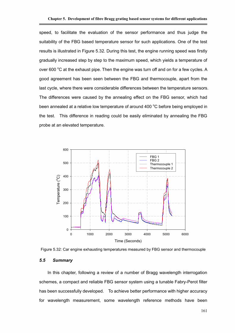
Chapter 5. Development of fibre Bragg grating based sensor systems for different applications
161
speed, to facilitate the evaluation of the sensor performance and thus judge the
suitability of the FBG based temperature sensor for such applications. One of the test
results is illustrated in Figure 5.32. During this test, the engine running speed was firstly
gradually increased step by step to the maximum speed, which yields a temperature of
over 600 oC at the exhaust pipe. Then the engine was turn off and on for a few cycles. A
good agreement has been seen between the FBG and thermocouple, apart from the
last cycle, where there were considerable differences between the temperature sensors.
The differences were caused by the annealing effect on the FBG sensor, which had
been annealed at a relative low temperature of around 400 oC before being employed in
the test. This difference in reading could be easily eliminated by annealing the FBG
probe at an elevated temperature.
5.5 Summary
In this chapter, following a review of a number of Bragg wavelength interrogation
schemes, a compact and reliable FBG sensor system using a tunable Fabry-Perot filter
has been successfully developed. To achieve better performance with higher accuracy
for wavelength measurement, some wavelength reference methods have been
Figure 5.32: Car engine exhausting temperatures measured by FBG sensor and thermocouple
Time (Seconds)
0 1000 2000 3000 4000 5000 6000
Tem
pe
ratu
re (
oC
)
0
100
200
300
400
500
600
FBG 1FBG 2
Thermocouple 1
Thermocouple 2

Optical fibre high temperature sensors and their applications
162
incorporated successfully into the system design and as a result the system has shown
a good wavelength resolution of 1 pm (equivalent to a temperature resolution of 0.1 oC),
with an absolute wavelength accuracy of better than 10 pm. Prior to the field tests, the
FBG sensor system was calibrated and cross-compared with the other types of optical
and electrical sensor systems when they were subjected to various environmental
conditions. The FBG system has shown advantageous characteristics for some
specific industrial applications and this has been confirmed by the positive results
obtained from various field tests.
Reference
[1]. A. Othonos and K. Kalli, “Fiber Bragg Gratings: Fundamnetals and Applications in
Telecommunication and sensing”, Artech House, 1999
[2]. S. M. Melle, K. Liu and R. M. Measures, “A passive wavelength demodulation system
for guided-wave Bragg grating sensors”, IEEE Photonics Technology Letters, Vol. 4,
1992, pp. 516-518
[3]. M. A. Davis and A. D. Kersey, “All-fibre Bragg grating strain sensor demodulation
technique using a wavelength division coupler”, Electronics Letters, Vol. 30, 1994, pp.
75-77
[4]. A. D Kersey, T. A. Berkoff, and W. W. Morey, “Multiplexed fiber Bragg grating strain
sensor system with a fiber Fabry-Perot wavelength filter”, Optics Letters, Vol. 18, 1993,
pp. 1370-1372
[5]. M. G. Xu, H. Geiger, J.L. Archambault, L. Reekie, J.P. Dakin, “Novel interrogation
system for fibre Bragg grating sensors using an acousto-optic tunable filter”,
Electronics Letters, Vol. 29, 1993, 99.1510-1511
[6]. D. A. Jackson, D. A. Jackson, A. B. Lobo Ribeiro, L. Reekie, and J. L. Archambault,
“Simple multiplexing scheme for fier optic grating sensor network”, Optics Letters, Vol.
18, 1993, pp. 1192-1194
[7]. Fabry C. and Perot A., “Sur les franges des lames minces argentées et leur
application á la mesure de petites épaisseur d’air”, Annales de Chimie et de Physique,
vol. 12, 1897, pp. 459 -501
[8]. H. Y. Tam, S. Y. Liu, et al., “Fiber Bragg Grating Sensors for Structural and Railway
Applications”, In Engineering Structures, International Society for Optical Engineering
(SPIE), Beijing, PR China, 2004, pp. 85-97.
[9]. S C Tjin, Y Wang, et al., “Application of quasi-distributed fibre Bragg grating sensors
in reinforced concrete structures”, Measurement Science and Technology, vol. 13,
2002, pp. 583
[10]. M.A. Davis, D.G. Bellemore, M.A. Putnam, A.D. Kersey, “Interogation of 60 fibre bragg
gratin sensors with microstrain resolution captivity”, Electronics letters Vol 32, 1996,
pp 1393-1394
[11]. S. E. Harris, R.W. Wallace, “Acousto-optic tunable filter”, Journal of Optics. Society

Chapter 5. Development of fibre Bragg grating based sensor systems for different applications
163
American, vol. 59, 1969, pp.744
[12]. M.S. Gottlieb, “Acousto-optic tunable filter, Design and Fabrication of Acousto-Optic
Devices”, Marcel Dekker, New York, 1994.
[13]. C. Boulet, , D.J. Webb, et al., “Simultaneous interrogation of fiber Bragg grating
sensors using anacoustooptic tunable filter”, Photonics Technology Letters, IEEE, Vol
13, 2001, pp1215-1217
[14]. D. C. C. Norman and D J Webb, “Fibre Bragg grating sensor interrogation using an
acousto-optic tunable filter and low-coherence interferometry”, Measurement
Sciences and Technology, Vol. 18, 2007, pp. 2967-2971
[15]. S. Tanaka, K. Yamada, H. Kobayashii, and M. Kadota “Application of Acoustooptic
Tunable Filter to Strain- or Vibration-Sensing System”, Japan Journal of Applied
Physics, Vol. 46, 2007, pp. 4633-4635
[16]. C, Antonio, “AOTF interrogation scheme for FBG”, Proc. SPIE Vol. 2722, Smart
Structures and Materials, 1996, pp.107-110
[17]. H. Gieger, M. G. Xu, J. P. Dakin, N. C. Eaton, and P. J. Chivers,., “Progress on grating
interrogation schemes using a tunable filter”, Proceedings of the Optical Fiber Sensor
Conference (OFS11), Sapporo, Japan, 1996, pp. 576-379
[18]. M. G. Xu, H. Geiber and J. P. Dakin, “Electronic tracking system for multiplexed fibre
grating sensors”, Electronics Letters, Vol. 31, 1995, 1228-1229
[19]. J. R. Dunphy, G.A. Ball, F.X. D'Amato, P. Ferraro, S. Inserra, A. Vanucci and M. Varasi,
“Instrumentation development in support of fiber grating sensor array”, Society of
Photo-optical Instrumentation Engineers, Distributed and Multiplexed Fiber sensors III,
Soston, 1993, Vol. 32071, pp. 2-11
[20]. G. P. Brady, et al., “Demultiplexing of fibre Bragg grating sensor with microstrain
resolution capability”, Optics Communications Vol. 11, 1994, pp. 51-54
[21]. M. A. Davis, Kersey, A.D “Matched-filter interrogation technique for fibre Bragg grating
arrays”, Electronics letters, Vol. 31, 1995, pp. 822-823
[22]. C. M. Tay, K.M. Tan, S.C. Tjin, C.C. Chan, “A high-resolution tunable fiber Bragg
grating filter” , Microwave and Optical Technology Letters, Vol. 42, 2004, pp. 89 - 92,
[23]. N. Mohammad, W. Szyszkowski, W. J. Zhang, E. I. Haddad, J. Zou, W. Jamroz, and R.
Kruzelecky, “Analysis and development of a tunable fiber Bragg grating filter based on
axial tension/compression”, Journal of Lightwave Technology, Vol. 22, 2004, pp. 2001-
2013
[24]. T. Coroy, M. N. Measures, “Active wavelength measurement system using an
InGaAs-InP quantum-well electroabsorption filtering detector”, IEEE Photonics
Technology Letters, Vol. 8, 1996, pp. 1686 - 1688
[25]. T. Coroy, Measures M. N, “Demodulation system for Bragg grating fiber optic sensors
using a quantum well electro-absorption filtering detector”, Smart Materials Structure,
Vol. 7, 1998, pp. 265-271
[26]. G. A. Ball, “Fibre Laser Source analyzer for Bragg grating sensor array interrogation”,
IEEE Journal of Lightwave Technology, Vol. 12, 1994, pp.700-703
[27]. M. A. Putman, M.L. Dennis, J.U. Kang, TE Tsai., “Sensor Grating demodulation using a
passively mode locked fibre laser”, Technical Digest Optical Fiber communications
Conference, Optical Society of America, Vol. 6, 1997, p.156.

Optical fibre high temperature sensors and their applications
164
[28]. M. L. Dennis, M. A. Putnam, J. U. Kang, T.E. Tsai, I.N. Duling III, and E.J. Friebele.,
“Grating sensor array demodulation by use of a passively mode-locked fibre laser”,
Optics letters, Vol. 22, 1997, pp. 138-140
[29]. X. Wan, H.F. Taylor, “Multiplexing of FBG sensors using mode locked
wavelength-swept fibre laser”, Electronics Letters, Vol. 39, 2003, pp.1512 – 1514
[30]. S. H. Yun, D.J. Richardson and B.Y. Kim,, “Interrogation of fibre Bragg arrays with a
wavelength swept fibre laser”, Optics Letters, Vol. 23, 1998, pp. 138-140.
[31]. Y. F. Takushima, F. Futami, K. Kikuchi,, “Generation of over 140 nm wide super
continuum from a normal dispersion fibre by using a mode-locked semiconductor
laser”, IEEE Photonics Technology Letters, Vol. 10, 1998, pp.1560-1562
[32]. S. J. Gong, G.H. LV, X.S. Li, X. Jiang, S.H. Shang, et. al., “A novel design of CCD
spectral detection circuit for FBG sensor interrogation”, Proceedings of SPIE, Vol.
6595(2), 2007, pp. 65953F.1-65953F.7
[33]. G. Y. Li, H. Zhang, B. Liu, J. Zhang, S.Z. Yuan, G.Y, Kai, X.Y. Dong, “The interrogation
system for FBG sensing based on the InGaAs linear image sensor”, Microwave and
Optical Technology Letters, Vol. 50, 2008, pp.1101 – 110
[34]. Uwe C. Mueller, Thomas Zeh, et Al., “Fiber optic Bragg grating sensors for
high-precision structural deformation control in optical systems”, Proceedings of SPIE
Vol. 6167, 2006, pp. 61670A.1-61670A.
[35]. C. G. Athkins, M. A. Putnam, and E. J. Friebele, “Instrumentation for interrogating
many-element fiber Bragg grating arrays embedded in fiber resin composites”,
Society of Photo-optical Instrumentation Engineers, Smarting Sensing Processing
and Instrumentation, 1995, Vol. 2444, pp. 257-266
[36]. A. D. Kersey, T. A. Berkoff, and W. W. Morey., “Interrogation and multiplexing
techniques for fibre Bragg grating strain sensors”, Society of Photo-Optical
Instrumentation Engineers, Distributed and Multiplexed Fiber Optic Sensors III,
Boston, Vol. 2071, 1993, pp. 30-48
[37]. A. D. Kersey. T.A. Berkoff, W.W. Morey, “High-resolution fibre grating based strain
sensor with interferometric wavelength-shift detection”, Electronics Letters, Vol. 18,
1992, pp. 1081-1083
[38]. W.R. Stephen, B.L.Bachim,,“Source-noise-induced resolution limits of interferometric
fibre Bragg grating sensor demodulation systems”, Measurement Science Technology
Vol. 12, 2001, pp.782-785
[39]. M. A. Davis and A. D. Kersey, “Fiber Fourier transform spectrometer for decoding
Bragg grating sensors”, Proceedings of the Optical Fibre Sensors Conference
(OFS10), Glasgow, UK, 1994, pp. 167-170
[40]. A. D. Kersey, T. A. Berkoff, and W. W. Morey ,“Fiber-optic Bragg grating strain sensor
with drift-compensated high-resolution interferometric wavelength-shift detection”,
Optics Letters, Vol. 18, 1993, pp72-74.
[41]. M. A. Davis and A. D. Kersey. “Application of a fiber Fourier transform spectrometer to
the detection of wavelength encoded signals from Bragg grating sensors”, IEEE
Journal of lightwave Technology, Vol. 13, 1995, pp. 1289-1295
[42]. G. Gagliardi, M Salza, P Ferraro and P De Natale, “Interrogation of FBG-based strain
sensors by means of laser radio-frequency modulation techniques”, Journal of optics.

Chapter 5. Development of fibre Bragg grating based sensor systems for different applications
165
A, Pure and applied optics, Vol. 8, 2006, pp. 507-513
[43]. Hydrogen Cyanide Gas Cell Datasheet, www. wavelengthreferences.com
[44]. W. Z. Zhao, T. Sun, K. T. V. Grattan, J. Lucas and A. I. Al-Shamma'a, "Temperature
monitoring of vehicle engine exhaust gases using optical fibre temperature sensor
systems", Proc. SPIE 5855, 2005, pp.832

Optical fibre high temperature sensors and their applications
166

Chapter 6. Fibre Bragg grating based fire alarm system
167
Chapter 6. Fibre Bragg grating based fire alarm system
6.1 Fluorescence-based and FBG-based fire alarm systems
In Chapter 3, a fluorescence-based temperature sensor system has been
specifically designed and evaluated for early fire detection, showing promise to be a
practical alternative to the conventional fire alarm system used in aero industries.
However the fluorescence-based system has some limitations, such as being sensitive
to light source fluctuation and to the locations of the temperature excursions, etc. The
FBG-based temperature sensor system, discussed extensively in Chapter 5, has shown
better performance for temperature measurement with higher accuracies, longer term
stability and insensitivity to environmental changes etc. Thus this Chapter describes
the extensive work undertaken to explore the potential and suitability of using a
FBG-based temperature sensor system for early fire detection.
As discussed in Chapter 4, FBGs written into conventional telecommunications
fibres cannot sustain elevated high temperatures and this has limited their applications
for high temperature measurements, such as for early fire detection in the aerospace
industry. However, as described in Chapter 4, when the gratings are written into some
specialist fibres, strong FBGs with high temperature sustainability (up to 900oC) can be
created and used for high temperature measurements. In particular, the recent
development by the research group at City University London of the novel Bi/Ge
co-doped fibres [1-3] has enabled strong FBGs to be written into, showing potential to
establish a FBG-based fire alarm system in order to better meet the requirements
highlighted in section 3.1.1.
6.1.1 FBG-based fire alarm system
The FBG-based fire alarm system is designed to measure the temperature of a hot
spot and the background temperature simultaneously, using a series of gratings written
into a single fibre, or a few fibres if more measurement channels are required. The
operational principle of the fire alarm system is similar to the FBG temperature sensor

Optical fibre high temperature sensors and their applications
168
system developed in Chapter 4 and system setup is illustrated in Figure 6.1. The probe
contains a series of FBGs written at the same wavelength, and when exposed to a
uniform background temperature, either being constant or varying, the spectral profile of
the reflected light from all the FBGs within the probe would have a single peak, as
shown in Figure 6.1(b). This single reflective Bragg wavelength, b, represents the
background temperature. When a hot spot, which has a different temperature
(normally higher) than that of the background, is present at any location along the probe,
a second reflective peak occurs, showing a different wavelength, h, corresponding to
the temperature of the hot spot as shown in Figure 6.1(c). Therefore, the temperatures
of the hot spot and the background can be derived from the wavelengths of these two
peaks based on equation (6.1).
, (6.1)
where Th, and Tb are the temperature of the hot spot and the background respectively.
Thus the background temperature and the temperature of hot spot can be measured
simultaneously, even when the background temperature varies. The temperature of
the hot spot has to be a certain degree higher than that of the background to be
detectable. This minimum detectable temperature difference between the hot spot and
the background is mainly determined by the overall bandwidth of the FBG series and
the resolution of the wavelength interrogation system. In this specific fire alarm system
developed, the minimum detectable temperature difference is about 30-40 oC, which is
sufficient for the particular application of aero engine temperature monitoring. The
sensor is placed inside a stainless tube to ensure the robustness of the probe for both
laboratory and field tests.
)( hh fT )( bb fT

Chapter 6. Fibre Bragg grating based fire alarm system
169
(a)
Figure 6.1: Experimental setup of the FBG-based fire alarm system
(a) Hardware setup. (b) Spectrum when FBGs are exposed to a uniform background
temperature. (c) Spectrum when a hot spot is present
6.1.2 System setup
Based upon the FBG-based temperature sensor system discussed in Chapter 5, a
prototype FBG-based fire alarm system was established and evaluated. As shown
schematically in Figure 6.2 and photographically in Figure 6.3, the system primarily
consists of:
Wavelength interrogation system
The hardware used for the FBG-based temperature sensor for wavelength
interrogation was also used in the fire alarm system without any major modifications.
This shows the flexibility of using an F-P filter scheme for wavelength interrogation
Broadband
source
Wavelength
Detection System
FBG1 FBG2 FBGm
Tb,bTb,b
2 x 1 coupler
b,h
Th,h
Plain fibre Plain fibre
Probe
Interface
software
FBGn
Tb,b
Hot spot
One Peak
T=T
Wavelength
Inte
nsi
ty
(b)
Two Peaks
T1=T(B)
T2=T(H)
Wavelength
Inte
nsi
ty
(c)
Background
Hot spot

Optical fibre high temperature sensors and their applications
170
Probe
The sensor probe has included three channels of FBG arrays, with each channel
containing 22~25 FBGs at a same wavelength in a single fibre of 1 meter length.
The difference between the channels is represented by their respective reflected
wavelengths, indicating which zone the hot spot is located.
Figure 6.2: Schematic of the FBG-Based fire alarm system
Figure 6.3: Experimental setup of the FBG-based fire alarm system
SLEDF-P tunable
filter
Photo
Detector
Amplifier
ADwin
DSP Card
Wavelength Scan
1 x 2 coupler
BroadBand Light Source
Interface Software
Photo
Detector
Amplifier
Gas Cell
Wavelength Reference
2 x 2 coupler FBG1 FBG2 FBGn
T,1T,1 T,1
FBG1 FBG2 FBGn
T,2T,2 T,2
FBG1 FBG2 FBGn
T,3T,3 Tn,3
Channel 1
Channel 3
Channel 2
Probe
Wavelength interrogation system
3-Channel probe
Interrogation system
Interface Software

Chapter 6. Fibre Bragg grating based fire alarm system
171
Interface Software
With some minor modifications, the interface software developed for the FBG
temperature sensor system can be used for the fire alarm system.
6.1.3 Probe fabrication
A probe comprising 3 FBG array channels was used for the preliminary test and
evaluation as a FBG-based fire alarm system. As illustrated above, each channel of
the probe contains an array of around 25 FBGs, uniformly spaced on a 4 cm interval in a
one-meter fibre. The 25 FBGs in the same array have the same back-reflected Bragg
wavelength, but have different wavelengths in different channels. Therefore in this work
the spectrum of the probe shows three different wavelengths representing three
different channels, when the probe is exposed to a uniform background temperature.
After the series of gratings being written into the fibre and subsequently being annealed
at a temperature of 250oC for over 24 hours, the sensing probe was then protected by
inserting into a single 1.2-meter steel tubing to ensure the robustness of the sensor for
further tests.
To ensure the fabrication of a series of gratings with the same Bragg wavelength for
each channel, it was essential to maintain the grating writing conditions, such as laser
energy and frequency, fibre tension, etc. This has been successfully achieved to
ensure that all the FBGs within the same channel have the same Bragg wavelength
within a fractional tolerance, thus enabling the overall bandwidth of all the FBGs in the
same channel to be kept within a certain defined range. This overall bandwidth is
correlated to the minimum detectable temperature difference between the hot spot and
the background. As illustrated in Figure 6.4, a -3dB bandwidth of each FBG array has
been achieved to be around 400pm, compared to ~200pm of a single FBG. This is due
to small overlaps of the spectra of the gratings. With such a bandwidth, the minimum
detectable temperature difference was calculted to be around 30oC, which satisfies the
industrial requirements for a fire alarm system as summarized in section 3.1.1.

Optical fibre high temperature sensors and their applications
172
Figure 6.4: Spectrum of a FBG array for the fire alarm probe
6.1.4 Interface software
Similar to the interface designed for the FBG-based temperature sensor system
discussed in Chapter 5, the interface software of the fire alarm system has built-in
functions for F-P filter controlling, wavelength data retrieving, analyzing and displaying,
thus providing a user-friendly interface. Some screen shots of the modified interface
software are shown in Figure 6.5. Figure 6.5 displays the temperatures of both the hot
spot, if present, and the background of three different channels monitored. A visual
alarm will be triggered whenever the measured temperature of the hot spot, in any
channel, is shown above the threshold (such as 50oC) above the temperature of the
background.
Wavelength (nm)
1532 1534 1536 1538 1540
Inte
nsity (
AU
)
B : 1536.411nm
BW(-3dB): 0.419nm

Chapter 6. Fibre Bragg grating based fire alarm system
173
Figure 6.5: Screen print out of the interface software for FBG fire alarm system
(Showing the graphic presentation of the temperatures of the hot spot and the background of
three channels)
6.2 Experimental tests and evaluation of the FBG-based fire alarm system
The prototype of the FBG-based fire alarm system developed at City University
London was subjected to a series of tests to evaluate its performance, in term of spatial
resolution, temperature resolution, response time and stability, etc, both in the
laboratory and in the industrial test environment.
6.2.1 Spatial resolution of the FBG-based fire alarm system
The spatial resolution termed here is not referring to the spatial resolution of the
hotspot location, which is distinguishable between different zones (channels) in a range
of 1 meter, but to a minimum detectable hot spot size. As discussed above, the
spacing between gratings within each channel is 4 cm therefore the minimum
detectable size should be 4cm to enable the temperature excursion to be detected by at
least one FBG. To verify this, the fire alarm system was used to record the
temperatures of the hot spot when the probe was exposed to various simulated hot
spots with different size and temperature profile at different locations. The simulated
hot spots were provided by two small heat sink blocks, one was 5 cm in length and the

Optical fibre high temperature sensors and their applications
174
other 2 cm. These heat sinks provided roughly uniform hot spots along their lengths
when heated by a heating element. The hot spot temperature readings were recorded
while the heat sinks were being moved along the fibre sensing length, while the
background temperature was kept at room temperature. The results are shown in
Figure 6.6. The readings with the 2 cm length heat sink fluctuated dramatically with
positions, while that with the 5 cm one was of relative small fluctuation. Such an
experiment was not carried out under the best test condition due to the limitation of
facility, however, it was clearly indicated that the minimum detectable hot spot size is
approximately equivalent to the spatial gap between the adjacent FBGs.
(a)
(b)
Figure 6.6: Spatial resolution of the FBG based fire alarm system under different stimulated
hotspots. (a) 5 cm heat sink (b) 2 cm heat sink
6.2.2 Temperature resolution of the FBG-based fire alarm system
Similar to the fluorescence-based fire alarm system developed and discussed in
Location (mm)
0 50 100 150 200
Tem
pera
ture
(oC
)
100
120
140
160
180
200
Location (mm)
0 50 100 150 200
Tem
pera
ture
(oC
)
40
60
80
100
120
140
160
180

Chapter 6. Fibre Bragg grating based fire alarm system
175
chapter 3, the minimum detectable temperature difference between the temperature of
the hot spot and that of the ambient background temperature is an important
specification for a FBG-based fire alarm system. As mentioned above, the minimum
detectable temperature difference of the system is mainly determined by the bandwidth
of the overall spectrum of the FBG array and the wavelength resolution of the
interrogation system. A simple experiment was carried out to verify this and to
determinate the minimum temperature difference which can be discerned by the system.
In this experiment, one sensing channel of the 3-channel system was kept at a room
temperature (~25oC) while one section (~5cm) of it was exposed to a heating element
simulating a hot spot. The spectra of the FBG array of the channel, as shown in Figure
6.7, were retrieved and recorded by the interrogation unit, while the temperature of the
heating element varied at room temperature, 50oC, 55oC and 100oC respectively. The
Figure 6.7: Spectrum of an FBG array of 24 FBGs, being placed at room temperature as
background and a section of 5cm exposed to a hot spot with a varying temperature of: (a) no hot
spot, (b) 50oC, (c) 55
oC, (d) 100
oC)
FBG Spectrum at Room temperature
(B: 1535.21nm)
Wavelength (nm)
1533 1534 1535 1536 1537 1538
Inte
nsity (
AU
)
FBGs spectrum atroom temperature
and 50oC hot spot
B=1535.30nm
Wavelength (nm)
1533 1534 1535 1536 1537 1538
Inte
nsity (
AU
)
FBGs spectrum atroom temperature
and 55oC hot spot
B1
:(1535.21nm)
B2
:(1535.52nm)
Wavelength (nm)
1533 1534 1535 1536 1537 1538
Inte
nsity (
AU
)
FBGs spectrum atroom temperature
and 100oC hot spot
nm
nm
Wavelength (nm)
1533 1534 1535 1536 1537 1538
Inte
nsity (
AU
)

Optical fibre high temperature sensors and their applications
176
results clearly indicated that the system could identify a hot spot of 55oC but not that of
50oC, which showed the minimum detectable temperature difference of the FBG based
fire alarm system was of 30oC, which is sufficient to meet the requirement of the
application for fire alarm detection of aircraft engine as detailed in the project.
6.2.3 Response time test of the FBG-based fire alarm system
The response time of the FBG-based fire alarm system was tested under a room
temperature background. A heat-gun was used to provide a hot spot over a spatial
region of < 10cm, with the maximum temperature achieved to be about 300oC. A typical
set of results obtained is shown in Figure 6.8, which is a printout from the interface
software. Figure 6.9 shows the results obtained from both the FBG-based fire alarm
system and from the K-type thermocouple (corresponding to the data circled in Figure
6.8). The results show the FBG-based fire alarm system had a response time of less
than one minute, which is much faster than that of the K-type thermocouple unit used for
comparison. It is also shown in Figure 6.9 that there is a sudden temperature drop to
the background temperature whenever the hot spot temperature is lower than 55oC,
30oC above the background temperature - this again confirms the minimum detectable
temperature difference between the hot spot and the background as observed in the
previous experiment. The system cannot identify the difference between the hot spot
and the background when their temperature difference is smaller than the minimum
detectable temperature difference.
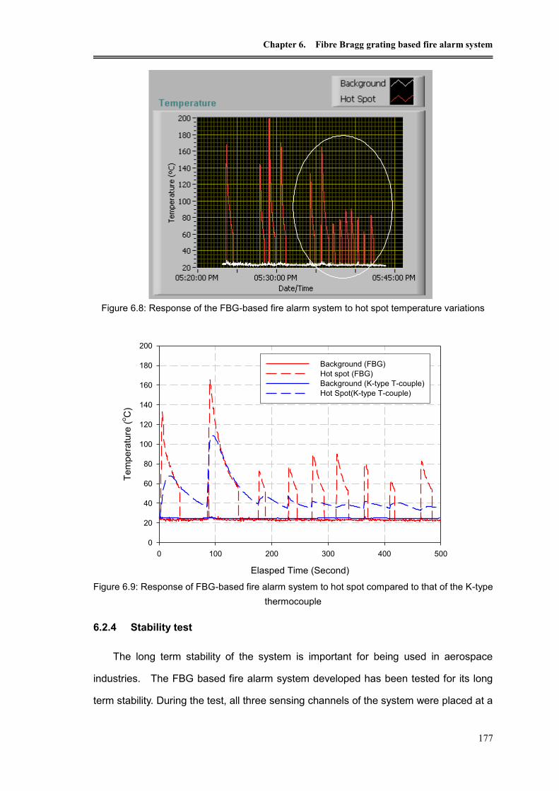
Chapter 6. Fibre Bragg grating based fire alarm system
177
Figure 6.8: Response of the FBG-based fire alarm system to hot spot temperature variations
Figure 6.9: Response of FBG-based fire alarm system to hot spot compared to that of the K-type
thermocouple
6.2.4 Stability test
The long term stability of the system is important for being used in aerospace
industries. The FBG based fire alarm system developed has been tested for its long
term stability. During the test, all three sensing channels of the system were placed at a
Elasped Time (Second)
0 100 200 300 400 500
Te
mp
era
ture
(oC
)
0
20
40
60
80
100
120
140
160
180
200
Background (FBG)
Hot spot (FBG)
Background (K-type T-couple)
Hot Spot(K-type T-couple)

Optical fibre high temperature sensors and their applications
178
room temperature environment while a small section of each channel was kept at a
temperature of 180oC using a small aluminium block with heating element, for around
45 hours. Then the heated sections were cooled naturally to the room temperature. The
results, together with readings from two thermocouples (with one for background
temperature measurement and the other for hot spot), are presented in Figure 6.10. It is
shown that the FBG based fire alarm system had a very stable reading during the
(a)
(b)
(c)
Figure 6.10: Long term stability test of the FBG based system
(a) Channel 1, (b) Channel 2, and (c) Channel 3
Elapsed time (h)
0 10 20 30 40 50
Tem
pe
ratu
re
0
20
40
60
80
100
120
140
160
180
200
Hot spot temp. - FBG probe
Hot spot temp. - Thermocouple
Background temp. - FBG probe
Background temp. - Thermocouple
Elasped time (h)
0 10 20 30 40 50
Te
mp
era
ture
(oC
)
20
40
60
80
100
120
140
160
180
Hot spot temp, - FBG probe
Hot spot temp. - Thermocouple
Background temp. - FBG probe
Background temp. - Thermocouple
Elasped time (h)
0 10 20 30 40 50
Te
mp
era
ture
(oC
)
0
20
40
60
80
100
120
140
160
180
200
Hot spot temp. - FBG probe
Hot spot temp. - Thermocouple
Background temp. - FBG probe
Background temp. - Thermocouple
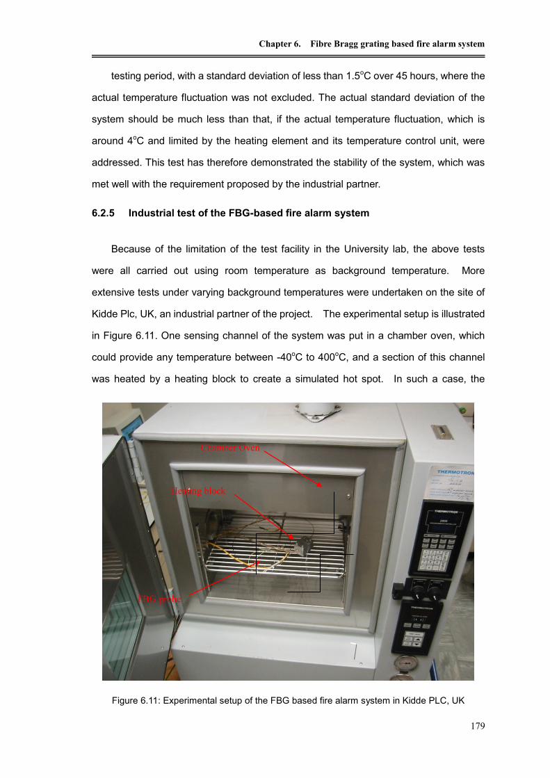
Chapter 6. Fibre Bragg grating based fire alarm system
179
testing period, with a standard deviation of less than 1.5oC over 45 hours, where the
actual temperature fluctuation was not excluded. The actual standard deviation of the
system should be much less than that, if the actual temperature fluctuation, which is
around 4oC and limited by the heating element and its temperature control unit, were
addressed. This test has therefore demonstrated the stability of the system, which was
met well with the requirement proposed by the industrial partner.
6.2.5 Industrial test of the FBG-based fire alarm system
Because of the limitation of the test facility in the University lab, the above tests
were all carried out using room temperature as background temperature. More
extensive tests under varying background temperatures were undertaken on the site of
Kidde Plc, UK, an industrial partner of the project. The experimental setup is illustrated
in Figure 6.11. One sensing channel of the system was put in a chamber oven, which
could provide any temperature between -40oC to 400oC, and a section of this channel
was heated by a heating block to create a simulated hot spot. In such a case, the
Figure 6.11: Experimental setup of the FBG based fire alarm system in Kidde PLC, UK
Chamber Oven
Heating block
FBG probe

Optical fibre high temperature sensors and their applications
180
temperature of the hot spot can be changed under a varied background temperature.
A series of tests was undertaken using the FBG based fire alarm system. The first
was to verify the system performance under varied ambient background temperature.
The ambient temperature, which is the temperature of the chamber oven, was set at
different values from -25oC to 100oC. The temperature of the hot spot was increased
from the background temperature to up to 200oC, which is simulated by the heating
block. Both the temperatures of the hot spot and of the background were recorded by
the FBG based fire system, and by thermocouples for calibration and cross-comparison.
A set of the typical results obtained is illustrated in Figure 6.12. The results showed that
the hot spot temperature readings of the FBG based system agreed well with those of
the thermocouple under different background temperature, except when the
background was set at -25oC. This discrepancy was believed to result from the use of
a temperature sensitivity of FBGs calibrated at temperatures above the room
temperature rather than that of lower temperatures. This deviation could be easily
eliminated by calibrating the sensor at lower temperatures, such as at -25oC in this
Figure 6.12: The hot spot temperatures measured by the FBG-based fire alarm system as a
function of those by a thermocouple under different background temperatures
Hotspot temperature - termocouple (oC)
0 50 100 150 200
FB
G m
easu
red h
ots
po
t te
mp
era
ture
(oC
)
0
50
100
150
200
250
Background at 100oC
Linear Regress 100oC
Background at 75oC
Linear Regress 75oC
Background at 30oC
Linear Regress 30oC
Background at -25oC
Linear Regress -25oC

Chapter 6. Fibre Bragg grating based fire alarm system
181
case.
Another experiment was carried out to evaluate the minimum detectable
temperature difference under different ambient background temperatures. The result,
illustrated in Figure 6.13, showed the minimum detectable temperature difference
decreased with increasing of ambient temperature. This meant a higher sensitivity at a
higher background temperature, which is desirable as the fire alarm system is mainly
designed to be used at elevated ambient temperatures, although this may result in a
more complicated calibration process to cover the wide range of the operating
temperature.
Figure 6.13: Minimum detectable temperature difference under different background
temperatures
6.2.6 Advantages over the fluorescence-based system
Compared to the fluorescence-based fire alarm system discussed in Chapter 3,
FBG-based sensor system has shown some advantages and these are highlighted
below.
Faster response time.
Due to the use of a complex signal processing algorithm to identify the very weak
fluorescence signal from the hot spot, the response time of fluorescence-based fire
Background temperature (oC)
-40 -20 0 20 40 60 80 100 120
Min
imu
m d
ete
ab
le t
em
pe
ratu
re (
oC
)
15
20
25
30
35
40
45
50

Optical fibre high temperature sensors and their applications
182
alarm system is limited to be around 2 seconds for the signal integration and data
processing. The response time of the FBG-based fire alarm system developed is
around 1 second, which is similar to that of a FBG temperature sensor system
discussed in Chapter 5. This can be further improved by using a smaller
packaging tubing to enable quick thermal transfer and a faster F-P scanning
frequency.
Higher accuracy
Compared to the fluorescence-based fire alarm system, the FBG-based system has
demonstrated a much higher accuracy for both the hot spot and the background
temperature measurements see Table 6.1 and Table 3.1.
Higher temperature resolution
The FBG-based fire alarm system has higher temperature resolution than the
fluorescence-based fire alarm system, especially for the hot spot temperature
measurement, also see Table 6.1 and Table 3.1.
Higher spatial resolution
The fluorescence based fire alarm system needs a certain section of fibre being
exposed to a hotspot to generate a detectable fluorescence signal and this limits its
spatial resolution to be a few centimetres. The special resolution of the FBG fire
alarm system is mainly limited by the distance between consequent FBGs, which is
about 4 cm in this case.
Insensitivity to light source fluctuation
The FBG-based fire alarm system is wavelength encoded, therefore
intensity-independent.
Insensitivity to hotspot location
The fluorescence-based fire alarm system is sensitive to the hot spot location as its
corresponding fluorescence signal varies with its location. The FBG-based

Chapter 6. Fibre Bragg grating based fire alarm system
183
system, however, is not sensitive to the hot spot location, but only its temperature.
Longer sensing fibre
The sensing fibre length of the fluorescence-based system is limited by the light
source intensity and the absorption losses when the fibre is pumped by light from a
laser diode to emit fluorescence. As shown in Figure 3.3, the fluorescence signal
generated from the middle section of the fibre would be very weak when the fibre is
of several meters and pumped from both ends. The FBG-based sensor system,
however, has demonstrated flexibility in writing required FBGs within any defined
sensing length, although there is a compromise between the sensing length and
spatial resolution of the system.
Ease of multiplexing
The sensing principle of the FBG-based fire alarm system is based upon the
multiplexing capability of FBGs, therefore the system is not limited only to detect
one hot-spot, but multiple ones. With the presence of several hot spots, the
fluorescence-based system would have some difficulty in deconvolving the
combined signals.
6.3 Summary
In this chapter, an FBG based fire alarm system was designed to offer an enhanced
and better performance over the fluorescence-based optical fibre fire alarm system
discussed in Chapter 3, taking the advantages of fibre Bragg gratings, such as faster
response, higher accuracy, higher spatial resolution, easy to be multiplexed, etc.
A prototype system of the FBG-based fire alarm system, together with a three
channel FBG array probe, was successfully built, tested and evaluated extensively, both
in the lab and in industry. The results have confirmed that the FBG based fire alarm
system has a better performance than that of the fluorescence based fire alarm system.
In summary, the system specifications achieved are listed in table 6.1. As
discussed in this chapter, the performance of the sensor system can be further

Optical fibre high temperature sensors and their applications
184
improved to meet the demands from aerospace applications.
Table 6-1: Specifications of the FBG-based fire alarm system
Spot measurement
precision
Background 2 oC
Hotspot 5 oC
Relative difference 4 oC
Minimum detectable temperature difference
between the hot spot and background
~35 oC
Probe length (22~25 FBGs in each channel) 3 x 1.5m
(1m sensing area)
Fibre material Ge-doped fibre
(or B-Ge co-doped fibre)
Operation temperature range 0~650 (oC)
Long term stability (oC, 24 hours) ~2
oC
Response time (second) 0.5~1
Light source output power (dBm / mW) 3 / 2
References
[1]. Y. Shen, T. Sun, K.T.V. Grattan and M. Sun, “Highly photosensitive Sb/Er/Ge codoped
silica fibre for fibre Bragg grating (FBG) writing with strong high-temperature
sustainability”, Optics Letters, Vol.28, 2003, pp.2025-2027
[2]. Y. Shen, J. He, T. Sun, K.T.V. Grattan, “High temperature sustainability of strong FBGs
written into Sb/Ge co-doped photosensitive fibre - decay mechanisms involved during
annealing”, Optics Letters, Vol.29, 2004, pp.554-556
[3]. Y. Shen, J. Xia, T. Sun and K.T.V. Grattan, “Photosensitive Indium doped
germano-silica fibre for strong FBGs with high temperature sustainability”, IEEE
Photonic Techology Letters, vol. 16, 2004, pp. 1319-1321

Chapter 7. Remote monitoring of FBG system using GSM short message
185
Chapter 7. Remote monitoring of FBG sensor system
using GSM short message
7.1 Application background
7.1.1 The need for a remote monitoring system
As discussed in previous chapters, FBG sensor systems have demonstrated
advantages over conventional techniques in many applications. In Chapters 5 and 6,
the FBG-based sensor systems developed at City University London have been used in
civil engineering, automotive industries, and aerospace. In addition to these applications,
FBG sensors can be and have been widely used for applications in wind energy,
offshore engineering, maritime, pipeline, power transformers. Most of in-situ
applications are carried out in the field where regular personnel on-site monitoring and
maintenance are not very convenient and sometimes very costly, but essential. For
such applications, a sensor system, which can somehow send the monitoring data and
operational conditions to a control centre, will be preferable and could be more efficient.
In this chapter, a remote monitoring system of FBG sensor using GSM short message is
presented. This remote sensor system can extend its application to many field
applications, and reduce the operation cost.
7.1.2 Wireless communication technologies
Wireless networks are becoming more pervasive, accelerated by new wireless
communication technologies and inexpensive wireless equipment. These networks are
transforming the way people use computers and other personal electronics devices at
work and home and when travelling. The wireless networks can also be used for remote
monitoring and controlling, and data communication of measurement instruments, such
as the case arises here for remote monitoring of FBG sensor system.
There are many wireless communication technologies, which can be differentiated
by the frequency, bandwidth, range, and applications. These technologies are generally

Optical fibre high temperature sensors and their applications
186
classified into four categories, depicted in Figure 7.1, in terms of coverage range [1].
The categories range from wireless personal area network (WPAN), which covers less
than 10 meters, to wireless wide area network (WWAN), which covers the widest global
area.
Figure 7.1: Wireless technologies categorized by range
Wireless Personal Area Network (WPAN) [1]
A Wireless Personal Area Network WPAN is a very small computer network used
for communications among computer devices (including telephones and personal digital
assistants) close to one person, which typically extend to 10 meters or less. Because of
their limited range, WPANs are used mainly as cable replacement technologies for data
synchronization and connectivity for device that are close to each other. Whilst USB and
FireWire are the commonly used cable technologies for personal area networks, the
wireless technologies of personal area networks are Bluetooth, IrDA (Infrared Data
Association), and High-bandwidth UWB (Ultrawideband).
Wireless Local Area Networks (WLAN) [1]
A Wireless Local Area Network (WLAN) is a wireless local area network, which is
the linking of two or more computers without using wires. In contrast to WPANs, WLANs
provide robust wireless network connectivity over a local area of approximately 100
meters between the access point and associated clients. Today’s WLANs are mainly
based on the IEEE 802.11 standard and are referred as Wi-Fi networks. 802.11b was
WLAN
Local Area Connectivity
100 meters
WPAN
personal Area Connectivity
10 meters
WMAN
Metro Area Connectivity
(City or suburb)
WWAN
Metro Area Connectivity
Broad geographic coverage

Chapter 7. Remote monitoring of FBG system using GSM short message
187
the first commercially successful WLAN technology. It operates in the 2.4 GHz
frequency band at 11 Mbps. By implementing a different data transmission method,
data transfer rate was increased to 54 Mbps with 802.11g in the 2.4 GHz band.
Wireless Metro Area Network (WMAN) [1]
A Wireless Metro Area Network (WMAN) is a wireless communication network that
covers a large geographic area, such as a city or suburb. It provides WLAN-like service,
primarily Internet access to an entire city. The best-known of these technologies of the
air interface for WMAN is IEEE 802.16d or “WiMax”, which operates in the 2-11 GHz
frequency range. The maximum data transfer rate under ideal conditions is 70 Mbps
over 50 kilometers.
Wireless Wide Area Network (WWAN) [1]
A Wireless Wide Area Networks (WWAN) is digital cellular networks for mobile and
data transmission, operated by network carries, such as Vodafone. WWAN covers a
much more extensive area than WLANs. They provided connectivity over a wide
geographical area. WWANs allow users to have access to the Internet, e-mail, and
corporate applications and information even being away from their office. But, until
recently, data rates of up to 115 Kbps have been relatively low compared to other more
localized wireless technologies. Two WWAN technologies, Global System for Mobile
Communication (GSM) and Code Division Multiple Access (CDMA), dominate the
WWAN deployments worldwide.
Europe standardized early on GSM technology. Nowadays, GSM and its
associated wireless data capability, General Packet Radio Service (GPRS) and the next
generation Enhanced Data GSM Evolution (EDGE), have about two-thirds of the world
wide market. The technologies have been widely deployed in North America, Europe,
and Asia. CDMA technology has seen strong deployments in North America, Japan,
Korea and China.
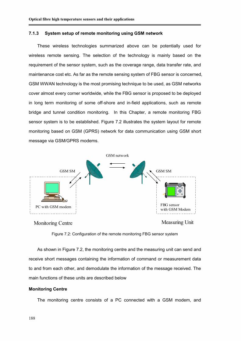
Optical fibre high temperature sensors and their applications
188
7.1.3 System setup of remote monitoring using GSM network
These wireless technologies summarized above can be potentially used for
wireless remote sensing. The selection of the technology is mainly based on the
requirement of the sensor system, such as the coverage range, data transfer rate, and
maintenance cost etc. As far as the remote sensing system of FBG sensor is concerned,
GSM WWAN technology is the most promising technique to be used, as GSM networks
cover almost every corner worldwide, while the FBG sensor is proposed to be deployed
in long term monitoring of some off-shore and in-field applications, such as remote
bridge and tunnel condition monitoring. In this Chapter, a remote monitoring FBG
sensor system is to be established. Figure 7.2 illustrates the system layout for remote
monitoring based on GSM (GPRS) network for data communication using GSM short
message via GSM/GPRS modems.
Figure 7.2: Configuration of the remote monitoring FBG sensor system
As shown in Figure 7.2, the monitoring centre and the measuring unit can send and
receive short messages containing the information of command or measurement data
to and from each other, and demodulate the information of the message received. The
main functions of these units are described below
Monitoring Centre
The monitoring centre consists of a PC connected with a GSM modem, and
PC with GSM modemFBG sensor
with GSM Modem
Monitoring Centre Measuring Unit
GSM network
GSM SM GSM SM
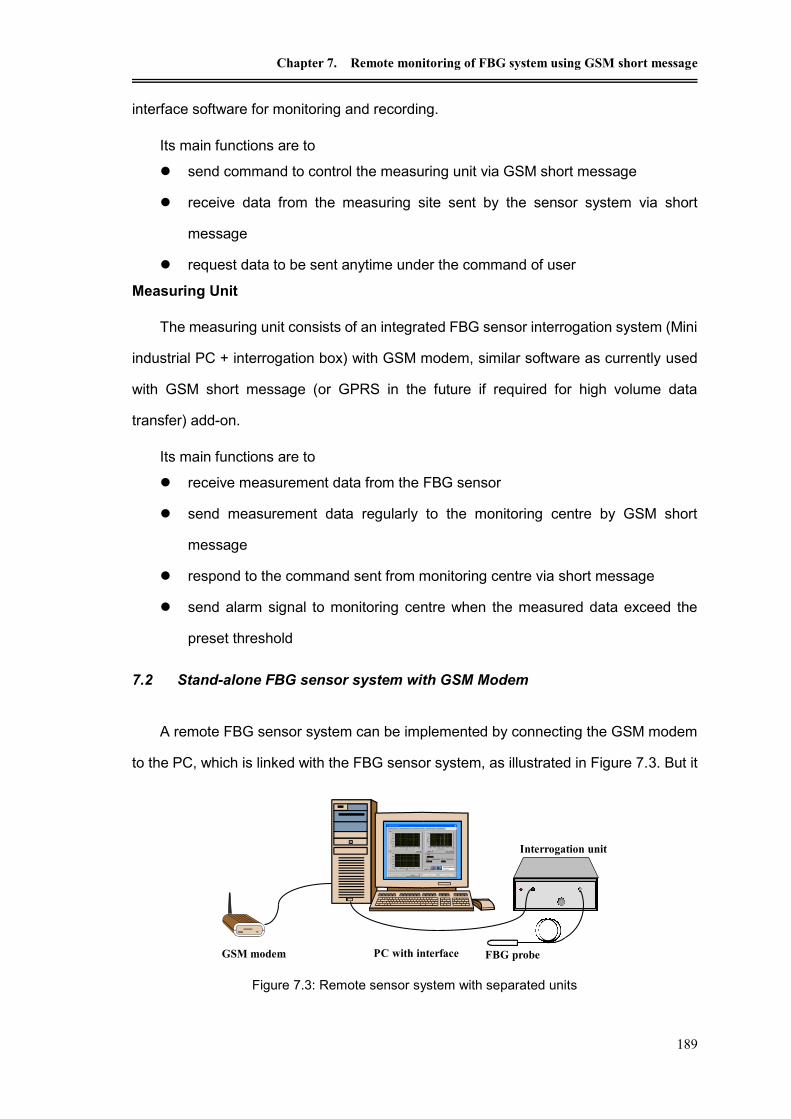
Chapter 7. Remote monitoring of FBG system using GSM short message
189
interface software for monitoring and recording.
Its main functions are to
send command to control the measuring unit via GSM short message
receive data from the measuring site sent by the sensor system via short
message
request data to be sent anytime under the command of user
Measuring Unit
The measuring unit consists of an integrated FBG sensor interrogation system (Mini
industrial PC + interrogation box) with GSM modem, similar software as currently used
with GSM short message (or GPRS in the future if required for high volume data
transfer) add-on.
Its main functions are to
receive measurement data from the FBG sensor
send measurement data regularly to the monitoring centre by GSM short
message
respond to the command sent from monitoring centre via short message
send alarm signal to monitoring centre when the measured data exceed the
preset threshold
7.2 Stand-alone FBG sensor system with GSM Modem
A remote FBG sensor system can be implemented by connecting the GSM modem
to the PC, which is linked with the FBG sensor system, as illustrated in Figure 7.3. But it
Figure 7.3: Remote sensor system with separated units
FBG probe
Interrogation unit
GSM modem PC with interface

Optical fibre high temperature sensors and their applications
190
will be much more convenient to integrate all the units into one compact box for remote
sensing in applications, e.g. for remote bridge monitoring.
In this project, a stand-alone sensor kit was created through the integration of the
FBG interrogation unit, a micro-industrial standard main-board together with a GSM
modem. The system built is shown in Figure 7.4. The main-board used was VIA VB6002
mini-ITX main-board, which is fully compatible with Microsoft® Windows® 2000/XP, CE
(a)
(b)
Figure 7.4: Integrated stand-alone remote FBG sensor system
(a) overview, (b) internal view
GSM
modem VB6002 mini-ITX
Probe
Wavelength
Interrogation unit
LCD touch screen

Chapter 7. Remote monitoring of FBG system using GSM short message
191
and XP, and Linux operating systems, from VIA Technologies Inc, Taiwan. A 6.5” TFT
LCD with touch screen was used for display and user interface for data input. With the
interface software being developed (discussed in the following sections), the kit has
been effectively used for stand-alone remote sensing applications.
7.3 Remote monitoring of FBG system using GSM short message technique
The measurement data of the FBG sensor system and the control information form
the monitoring centre are communicated using GSM short message through the GSM
modem. In the following sections, the methods of sending and receiving short
messages using a PC via the GSM modem are discussed.
7.3.1 Introduction of GSM AT command
Most of the GSM modems (and mobile phones) can support the AT command set
by GSM 07.05, which is published by European Telecommunications Standards
Institute (ETSI) [2]. It includes the control of the Short Message Service (SMS). The
main AT commands related to SMS and used in this project are listed in Table 7.1. A PC
thus can control the GSM modem (or mobile) by sending AT commands to it via COM
port.
Table 7-1: Main SMS AT commands
AT+CMGR Read SMS message
AT+CMGS Send SMS message
AT+CMGC Send an SMS command
AT+CMGD Delete SMS message
AT+CMGF Select SMS message format
AT+CMGL List SMS message from preferred store
AT+CMGW Write SMS message to memory
AT+CMSS Send SMS message from storage
AT+CNMI New SMS message indications
AT+CPMS Preferred SMS message storage
AT+CSCA SMS service centre address

Optical fibre high temperature sensors and their applications
192
AT+CSMP Set SMS text mode parameters
AT+CSMS Select Message Service
7.3.2 Sending and receiving message using a PC via GSM modem in Protocol
Data Unit (PDU) mode
7.3.2.1 Short message modes
There are three interface protocols, termed as SMS block mode, SMS text mode
and SMS PDU (Protocol Data Unit) mode, of a GSM Modem or mobile phone[4]. The
mode that a GSM/GPRS modem or mobile phone is operating determines the syntax of
some SMS AT commands and the format of the responses returned after execution.
Text mode is simpler to implement but has some limitations, conversely, PDU mode
is more difficult to implement but more flexible. In this project, the PDU Mode was used
for sending and receiving the short messages.
7.3.2.2 Receiving a message in the PDU mode
When a new message arrives, the following AT command is used to read it form
MT.
AT+CMGR = Index (index is the index number of the ME storage where the
message is saved)
The MT responds to the following messages to the TE, which include the PDU
string.
The PDU string contains not only the message, but also a meta-information about
the sender, SMS Centre, the time stamp etc. It is all in the form of hex-decimal octets or
decimal semi-octets. The construction of the PDU string is detailed in Table 7.2 [2].

Chapter 7. Remote monitoring of FBG system using GSM short message
193
Table 7-2: Structure of the PDU string of a received message
Octet(s) Description
07 Length of the SMSC information (in this case 7 octets)
91 Type-of-address of the SMSC. (91 means international format of the
phone number)
72 38 01 00 10 F5 Service centre number (in decimal semi-octets). The length of the
phone number is odd (11), so a trailing F has been added to form
proper octets. The phone number of this service centre is
"+27831000015".
04 First octet of this SMS-DELIVER message.
0B Address-Length. Length of the sender number (0B hex = 11 dec)
C8 Type-of-address of the sender number
72 38 88 09 00 F1 Sender number (decimal semi-octets), with a trailing F
00 TP-PID. Protocol identifier.
00 TP-DCS Data coding scheme
99 30 92 51 61 95 80 TP-SCTS. Time stamp (semi-octets)
0A TP-UDL User data length, length of message. The TP-DCS field
indicated 7-bit data, so the length here is the number of septets (10).
If the TP-DCS field were set to indicate 8-bit data or Unicode, the
length would be the number of octets (9).
C8329BFD0E01 TP-UD. Message "Hello!", 8-bit octets representing 7-bit data.
All the octets above are hex-decimal 8-bit octets, except the Service Centre number,
the sender number and the timestamp; they are decimal semi-octets. The message part
in the end of the PDU string consists of hex-decimal 8-bit octets, but these octets
represent 7-bit data, PDU encoded (discussed later).
7.3.2.3 Sending a message in the PDU mode
The following example shows how to send the message "hello!" in the PDU mode
AT+CMGF=0 //Set PDU mode
AT+CMGS=23 //Send message, 23 octets (excluding the two initial zeros)
MT responses: >
TE sends: 0011000B916407281553F80000AA0AE8329BFD4697D9EC37
There are 23 octets in this message (46 'characters'). The first octet ("00") doesn't
count, it is only an indicator of the length of the SMSC information supplied (0). The
PDU string consists of the following information:

Optical fibre high temperature sensors and their applications
194
Table 7-3: Structure of the PDU string of a sent message
Octet(s) Description
00 Length of SMSC information. Here the length is 0, which means that
the SMSC stored in the phone should be used.
11 First octet of the SMS-SUBMIT message.
00 TP-Message-Reference. The "00" value here lets the phone set the
message reference number itself.
0B Address-Length. Length of phone number (11)
91 Type-of-Address. (91 indicates international format of the phone
number).
6407281553F8 The phone number in semi octets (46708251358). The length of the
phone number is odd (11), therefore a trailing F has been added, as
if the phone number were "46708251358F". Using the unknown
format (i.e. the Type-of-Address 81 instead of 91) would yield the
phone number octet sequence 7080523185 (0708251358). Note
that this has the length 10 (A), which is even.
00 TP-PID. Protocol identifier
00 TP-DCS. Data coding scheme. This message is coded according to
the 7bit default alphabet. Having "02" instead of "00" here, would
indicate that the TP-User-Data field of this message should be
interpreted as 8bit rather than 7bit (used in e.g. smart messaging,
OTA provisioning etc).
AA TP-Validity-Period. "AA" means 4 days. Note: This octet is optional,
see bits 4 and 3 of the first octet
0A TP-User-Data-Length. Length of message. The TP-DCS field
indicated 7-bit data, so the length here is the number of septets (10).
If the TP-DCS field were set to 8-bit data or Unicode, the length
would be the number of octets.
C8329BFD0E01 TP-User-Data. These octets represent the message "Hello!". How to
do the transformation from 7bit septets into octets is shown here
7.3.2.4 PDU encode
For sending a short message in PDU mode, the user’s message is required to be
transformed into PDU string, namely PDU encoded. However the whole message to be
sent includes some other information as mentioned above. This transformation is
described in detail in GSM 03.38. The following shows how the message “Hello!” is
transformed into PDU string, as an example.
The message "hello!" consists of 6 characters, called septets when represented by

Chapter 7. Remote monitoring of FBG system using GSM short message
195
7 bits each. These septets need to be transformed into octets for the SMS transfer. This
transforming process is shown in Table 7.4. The transformation is based on the 7 bit
default alphabet, but an application built on the PDU mode can use any character
encoding.
Table 7-4: process of encoding message into PDU string
The first septet 1001000 (“H”) is turned into an octet by adding the most right bit of
the second septet. This bit is inserted to the left which yields 1 + 1001000 = 11001000
("C8"). The most right bit of the second septet 1100101 of the second character (“e”) is
then consumed, so it needs two bits of the third septet to make an 8 bit octet. This
process carries on until the last character. Leading 0s are added if the last octet has less
than 8 bits. The octets are then turned into hex, and hence the original message “Hello!”
is transformed into the 8-bit octets PDU string “C8329BFD0E01”.
7.3.2.5 PDU decode
While receiving a message sent in PDU mode, the message is PDU encoded and is
needed to be transformed into normal string, thus to interpret 8-bit octets as 7-bit
messages. The following shows how 8-bit octets PDU string “C8329BFD0E01” is
decoded to 7-bit message “Hello!”.
Original String H e l L O !
Original Hex 0x48 0x65 0x6C 0x6C 0x6F 0x21
Original binary 01001000 01100101 01101100 01101100 01101111 00100001
Original septet 1001000 110010 1 11011 00 1101 100 110 1111 01 00001
Coding process
Object Octet 1 1001000 00 110010 100 11011 1111 1101 00001 110 000000 01
Object Hex 0xC8 0x32 0x9B 0xFD 0x0E 0x01
Object String C8329BFD0E01

Optical fibre high temperature sensors and their applications
196
Table 7-5: process of decoding PDU string into message string
The first octet 11001000 (0xC8) is turned into a septet by moving the most
significant bit (MSB) 1, resulting in 1001000 (0x48). The removed MSB is then added to
the right of the second octet while removing the most left 2 bits into the next septet to
yield 110010 + 1 = 1100101 (0x65). This process carries on until the last character.
Leading 0s of the last octet are removed. The septets are then turned into hexes and
their ASCII letter accordingly. Therefore the 8-bit octets PDU string “C8329BFD0E01” is
transformed into message “Hello!”.
7.3.2.6 Instant message reading
As discussed in the previous sections, the TE (a PC) can send and receive short
messages from GSM modem by controlling it with AT commands. Among these AT
commands, the PC sends an initiative enquiry command to receive/read message form
the GSM modem. For example, TE sends “AT+CMGL” command, MT then replies with
the received and saves message(s); TE sends “AT+CMGR=<index>”, and MT replies
with the message saved at <index>. This kind of enquiring and retrieving method is the
operational principle of AT commands. However, these are some limitations in real
applications.
When receiving a message, MT saves it, and sends it to TE when requested, there
will be a delay between them, which depends on the enquiry frequency.
When TE sends the requesting AT command “AT+CMGL”, TE will receive the final
“OK” signal from MT, no matter whether the MT has the message or how many
messages it has. This results in a long period of waiting, normally of 5-10
Original String C8329BFD0E01
PDU Hex 0xC8 0x32 0x9B 0xFD 0x0E 0x01
PDU binary 1 1001000 00 110010 100 11011 1111 1101 00001 110 000000 01
Coding process
Object septet 1001000 110010 1 11011 00 1101 100 110 1111 01 00001
Object Oct 0100100 01100101 01101100 01101100 01101111 00100001
Object Hex 0x48 0x65 0x6C 0x6C 0x6F 0x21
Object String H E l L O !

Chapter 7. Remote monitoring of FBG system using GSM short message
197
seconds.
For many applications, this type of delay is undesirable as frequent enquiries
occupy lots of CPU resource. Therefore, a technique of “instant” receiving/reading
message was introduced. When MT receiving a message, it will inform TE or send it to
TE automatically. It works like an interrupt rather than the enquiry mechanism discussed
above.
Most of GSM modems support a AT command “AT+CNMI”, to select the procedure
of how to receive new messages from the network and TE is informed of this when TE is
active, e.g. through sending indication to TE or forwarding message to TE directly.
There are different modes of using command “AT+CNMI”, Please refer GSM 07.05
standard for details [4]. In this project, the mode of “AT+CNMI=2, 1” is used. In this
mode, when TE receive the indication “+CMTI” of new message from MT, it sends
“AT+CMGR” command to read the message context form MT.
7.4 Interface Software
Based on the technique for sending and receiving SMS discussed above, the
interface software for both the monitoring centre and the FBG sensor kit with GSM
function add-on was developed using Labview platform.
7.4.1 GSM add-on software module for the sensor kit
As the main FBG wavelength interrogation unit in the stand-alone system stems
from the FBG-sensor system developed and discussed in Chapter 4, the interface
software for the FBG-based sensor system can be easily modified to be used in the
stand-alone sensor kit. However, an add-on module requires the interface software to
be developed for data transfer using GSM short message to enable the remote sensor
system to be created.
As shown in Figure 7.7, the GSM add-on module provides the following main
functions:
Configures for GSM modem communication
Encodes the measurement result into PDU string

Optical fibre high temperature sensors and their applications
198
Decodes the control message (in PDU string) sent by the monitoring centre
Automatically sends data to the monitoring centre or any other predefined user
at a desired period. This function can also be turn on and off by the monitoring
centre, remotely.
Sends alarm data when the value exceeds the threshold. This function can also
be turn on and off by the monitoring centre.
Actively sends measurement data as a short message to a receiver, e.g.
monitoring centre or a mobile phone.
Responds to a data acquisition request.
In addition to these features, other functions, such as remote control and set the
sensor kit operation, remote system diagnose, etc., can be easily added on, to provide
full functional remote controlling and monitoring.
Figure 7.5: Screen printout of the GSM add-on module of the stand alone FBG sensor kit
7.4.2 User interface software for remote monitoring centre
The remote sensor kit with GSM add-on module can simply be controlled and
monitored by a mobile phone through short message communications. However, a

Chapter 7. Remote monitoring of FBG system using GSM short message
199
dedicated monitoring centre with appropriate program is able to provide the following
desirable functions.
Encodes and sends command, such as switch on and off, set data sending
frequency, alarm threshold hold, to control the measuring kit via GSM short
message.
Gets and decodes data from the measuring site sent by the sensor system via
short message.
Requests data to be sent anytime under the command of user.
Presents and manages the measurement data as a real-time system.
The initial user interface software was programmed using Labview platform, with
the front panels being shown in Figure 7.8.

Optical fibre high temperature sensors and their applications
200
Figure 7.6: Front panel of monitoring centre interface software
7.5 Summary
Driven by the motivation of potential applications for remote field measurement and
monitoring of the FBG based system, the GSM short message technology was explored
in this work to facilitate the wireless sensing and monitoring with FBG sensor system.
The technique of using PC to send and receive short messages is briefly discussed and
implemented with the software developed on the Labview platform.
Subsequently a stand-alone FBG sensor kit was developed with the intention of
field applications in remote areas, such as off-shore applications and remote bridge
monitoring applications. User interface software for a monitoring centre has also been
developed in association with the remote measurement system.
This method of utilising GSM short message technology used in this work for
remote sensing is generic and can be easily adapted for other wireless sensing
applications, which do no require huge amount of data transfer but require wide range
coverage.

Chapter 7. Remote monitoring of FBG system using GSM short message
201
Reference
[1]. Liam Quinn, Pratik Mehta, Alan Sicher “Wireless communications technology
landscape”, white paper, Feb 2005, Dell.
[2]. GSM_07.05_Specification, European Telecommunication Standard, ETS 300 585,
April 1997

Optical fibre high temperature sensors and their applications
202
Chapter 8. Conclusions and future work
203
Chapter 8. Conclusions and future work
8.1 Summary of the major achievements
The main work of this thesis focused on the development of two major optical fibre
sensor systems: novel fibre temperature sensor system based on the fluorescence
decay lifetime thermometry and FBG sensor system based on strong FBGs written into
novel photosensitive fibres. Based on the fundamental theoretical analysis, much of
the emphasis and effort was on the realization of the sensor systems through
experimental practices, i.e. by building and evaluating an optical fibre sensor system for
practical industrial applications. As a result, several sensor systems have been
successfully designed, created, tested and evaluated with an aim to meet the
specifications identified by industrial partners. Thus the major achievements and
innovations of this work are summarized and listed below.
1. A robust fluorescence lifetime-based optical fibre sensor system has been
successfully developed, with the implementation of phase-locked detection
(PLD) signal processing scheme and microchip unit for period measurement. In
this work, the Tm doped YAG crystal was selected as a sensing material to
construct the fluorescence-based thermometer. Its strong signal and long
fluorescence lifetime over the temperature range from room temperature to
above 1000oC enabled the thermometer to cover a wide temperature sensing
range with a relatively high resolution, showing good repeatability and long term
stability [1,2].
2. An optical fire alarm system, based on double exponential fluorescence lifetime
measurement using data fitting method, was developed and evaluated. It has
demonstrated the potential of their applications in aero industry [3]. However,
the system showed certain level of limitations for practical applications.
3. A novel photosensitive fibre, Bi/Ge co-doped fibre, has been designed and

Optical fibre high temperature sensors and their applications
204
fabricated specifically for the creation of strong FBGs for high temperature
applications. The photosensitivity and thermal characteristics of fibre Bragg
grating inscribed into this novel fibre have been tested and evaluated. The
results show that the strong gratings written into the Bi/Ge fibre can retain high
reflectivity after being annealed at elevated temperatures over 900 oC, therefore
are well suited for high temperature applications [4].
4. A compact and reliable FBG sensor system based on a tunable Fabry-Perot
filter was built. The system has shown a good wavelength resolution of 1 pm
(equivalent to a temperature resolution of 0.1 oC), with an absolute wavelength
accuracy of better than 10 pm. Following successfully testing in several field
applications, the system has been verified to be well suited for in-situ monitoring
[5].
5. A prototype system of the FBG-based fire alarm system together with a three
channel FBG array probe, were built and evaluated, both in the lab and in
industry. The results have indicated that the FBG based fire alarm system has
shown a better performance, in terms of faster response, higher accuracy,
higher spatial resolution, easier to be multiplexed, than that of the fluorescence
based fire alarm system. The FBG based fire alarm system has shown promise
and several key advantageous features for aerospace applications.
6. Driven by the motivation of potential application in the remote field
measurement and monitoring of the FBG based system, the GSM short
message technology was explored to enable the wireless sensing and
monitoring with FBG sensor system. The technique of using PC to send and
receive short messages is briefly discussed and implemented with the interface
software being developed on the Labview platform.
7. A stand-alone FBG sensor kit integrated with GSM short message technology
for wireless sensing and monitoring was developed with the intention of field
applications in remote areas, such as off-shore and remote bridge monitoring.
User interface software for a monitoring centre has also been developed in

Chapter 8. Conclusions and future work
205
association with the remote measurement system.
In summary, with reference to the aims and objectives set out in Chapter 1, all of the
following were achieved and delivered.
A fluorescence based optical thermometer, with its user interface software, was built
and evaluated
A fluorescence based optical fibre alarm system was developed and tested
A novel photosensitive fibre was fabricated, and characteristics of the strong FBGs
written into this were studied.
A compact and reliable FBG sensor interrogation system was developed and
applied in several applications.
A FBG based fire alarm system was built and test both in laboratory and industries.
Remote sensing system utilizing the GSM technology was studied. A stand-alone
FBG sensor kit developed.
Results obtained have been reported in the peer reviewed literatures and at
international conferences.
8.2 Suggestions for the future work
This thesis covers the details of the development of a wide range of optical fibre
sensor systems and their key technologies being used. The work has been mainly
focused on the practical aspects of the sensor system, further work could be on the
theoretical research and simulation, which may provide good guidance for the sensor
system performance improvement and optimization.
As an example, in the field of fluorescence lifetime based thermometry, a detailed
investigation of the concentration of Tm dopant in the YAG crystal would be valuable in
obtaining a better knowledge of the concentration dependence of the fluorescence
lifetime and the fluorescence intensity, and thus providing an effective means of
optimizing the probe through the selection of a sensor material with an appropriate
dopant concentration.

Optical fibre high temperature sensors and their applications
206
For the FBG based optical fibre systems, further work should be focused on two
aspects: novel photosensitive fibres and the wavelength interrogation system.
Through some theoretical modelling, more thermal-sustainable photosensitive fibres,
such as the Bi doped fibres discussed in the thesis, with optimized compositions may be
realized. It is also important to increases the resolution and accuracy of the sensor
system through the improvement on the wavelength interrogation algorithms.
Finally, the GSM technique employed for the FBG-based remote sensing system
can and should be further incorporated into some other sensor systems to create more
remote sensing systems due to its generic nature.
Reference
[1]. Y. H. Shen, W. Z. Zhao, J. L. He, et al., “Fluorescence decay characteristic of
Tm-doped YAG crystal fibre for sensor applications, investigated from room
temperature to 1400°C”, IEEE Sensors Journal, vol. 3, 2003, pp. 507-512
[2]. Y. H. Shen, W. Z. Zhao, et al., “Characterization of an optical fibre thermometer
using Tm3+:YAG crystal, based on the fluorescence lifetime approach”, Sensors
and Actuators, A: Physical, vol. 109, 2003, pp. 53-59
[3]. Y. H. Shen, J. l. He, W. Z. Zhao, et al., "Thermal decay characteristics of strong fiber
Bragg gratings showing high-temperature sustainability," J. Opt. Soc. Am. B Vol. 24,
2007, pp.430-438
[4]. W. Zhao, Y. Shen, T. Sun, and K. T. V. Grattan, " FBGs in Bi-Ge Co-doped
Photosensitive Fibre for High Temperature Measurement up to 1000ºC," in Optical
Fiber Sensors, OSA Technical Digest (CD) (Optical Society of America, 2006), paper
TuE86.
[5]. W. Z. Zhao, T. Sun, and K. T. V. Grattan, et al., “Nd-doped fluorescent fibre fire alarm
system based on signal regression approaches”, OFS(16), 2003, TuP-30
[6]. W. Z. Zhao, T. Sun, et al., “Temperature monitoring of vehicle engine exhaust gases
under vibration condition using optical fibre temperature sensor systems” ,Journal of
Physics: Conference Series, Vol. 45, 2006, pp.215

Relevant Publications by the Author
207
Appendix: Relevant publications by the author
A. Papers published in journals
[1]. Y. H. Shen, W. Z. Zhao, et al., “Fluorescence decay characteristic of Tm-doped
YAG crystal fibre for sensor applications, investigated from room temperature to
1400°C”, IEEE Sensors Journal, Vol. 3, 2003, pp. 507-512
[2]. Y. H. Shen, S. Y. Chen; W. Z. Zhao, et al., Growth characteristics and potential
applications in optical sensors of composite Cr4+:yttrium-aluminum-garnet
(YAG)-Nd3+:YAG crystal fibre”, Review of Scientific Instruments, Vol. 74, 2003,
pp.1187-1191
[3]. Y. H. Shen, W. Z. Zhao, T. Sun, K. T. V. Grattan, “Characterization of an optical
fibre thermometer using Tm3+:YAG crystal, based on the fluorescence lifetime
approach”, Sensors and Actuators, A: Physical, Vol. 109, 2003, pp. 53-59
[4]. Y. H. Shen; J. L. He; W. Z. Zhao, et al. “Fibre-optic sensor system for heat-flux
measurement”, Review of Scientific Instruments, Vol. 75, 2004, pp.1006-1012
[5]. Y. H. Shen, J. l. He, W. Z. Zhao, et al., "Thermal decay characteristics of strong
fiber Bragg gratings showing high-temperature sustainability," J. Opt. Soc. Am. B
Vol. 24, 2007, pp.430-438
[6]. Y. H. Shen, Y. Q Qiu, W. Z. Zhao, et al., "Short cavity single frequency fiber laser for
in-situ sensing applications over a wide temperature range," Optical Express Vol.
15, 2007, 363-370
[7]. S. Y. Chen, T. L. Yeo, W. Z. Zhao, et al., “Development of multi-wavelength
microsphere fibre laser system for potential sensor applications”, Optics
Communications, Vol. 282(3), 2009, pp. 401-405
[8]. E Lewis, G Dooly, E Hawe, C Fitzpatrick, P Chambers, J Clifford, W.Z Zhao, T Sun,
K.T.V Grattan and J Lucas, et al. “Overview of the OPTO-EMI-SENSE Project:
Optical Fibre Sensor Network for Automotive Emission Monitoring”, Sensors, Vol.
21(II), 2008, pp. 179-196
[9]. H Dong, W. Z. Zhao, T Sun, et al. Vibration-insensitive temperature sensing
Optical fibre high temperature sensors and their applications
208
system based on fluorescence decay and using a digital processing approach,
Measurement Science and Technology, Vol. 17, 2006, pp. 2010
B. Papers presented in conferences
[1]. Y. H. Shen, W. Z. Zhao, J. L. He, T. Sun, K.T.V. Grattan,“Fibre thermometer
based on the cross detection of the fluorescent decay of Tm:YAG crystal fibre and
background radiation”, SPIE Proceedings, Vol. 4920, 2002, pp.16-24
[2]. Y. H. Shen, S. Y. Chen, W. Z. Zhao, J. Chen. “Composite Cr 4+:YAG- Nd3+:YAG
crystal fibre: growth characteristics and passively Q-switched laser operation”,
Proceedings of SPIE, Vol. 4918, 2002, pp.20-9
[3]. L. H. Ye, Y. F. Zhang, W. Z. Zhao, Y. H. Shen. “Sapphire fibre thermometer
based on fluorescence lifetime measurement”, Proceedings of SPIE, Vol.4920,
2002, pp.25-30
[4]. Y. H. Shen, W. Z. Zhao, Jinglei He, et al., “Fibre thermometer based on the cross
detection of the fluorescence decay of Tm:YAG crystal fibre and background
radiation”, Proceedings of SPIE, Vol.4920, 2002, pp.16-24
[5]. W. Z. Zhao, Y. H. Shen, et al., “Precision free electron laser materials adhesion
monitoring using an optical fibre temperature sensor system”, OFS(16) 2003,
Tu4-4.
[6]. W. Z. Zhao, T. Sun, and K. T. V. Grattan, et al., “Nd-doped fluorescent fibre fire
alarm system based on signal regression approaches”, OFS(16), 2003, TuP-30
[7]. W. Z. Zhao, T. Sun, et al., "Temperature monitoring of vehicle engine exhaust
gases using optical fibre temperature sensor systems", Proc. SPIE 5855, 2005,
pp.832
[8]. J. Mulrooney, J. Clifford, C. Fitzpatrick, E. Lewis, W. Z. Zhao, T. Sun, K. T. V.
Grattan, et al., "Optical fibre sensors for the monitoring of harmful emissions from
land transport vehicles", Proc. SPIE 5826, 2005, pp. 586
[9]. W. Z. Zhao, T. Sun, et al., “Temperature monitoring of vehicle engine exhaust
gases under vibration condition using optical fibre temperature sensor
Relevant Publications by the Author
209
systems” ,Journal of Physics: Conference Series, Vol. 45, 2006, pp.215
[10]. M. O'Farrell, C. Sheridan, E. Lewis, W. Z. Zhao, T. Sun and K. T. V. Grattan, "An
integrated probe design for measuring food quality in a microwave environment",
Proc. SPIE 6619, 2007, p. 66190N
[11]. W. Z. Zhao, Y. H. Shen, T. Sun, and K. T. V. Grattan, "FBGs in Bi-Ge Co-doped
Photosensitive Fibre for High Temperature Measurement up to 1000ºC," in Optical
Fiber Sensors, OSA Technical Digest (CD) (Optical Society of America, 2006),
paper TuE86.
[12]. S K T Grattan, P A M Basheer, S E Taylor, W. Z. Zhao, et al., “Corrosion induced
strain monitoring through fibre optic sensors”, Journal of Physics: Conference
Series, Vol. 85, 2007, 012017
C. Patents
[1]. K.T.V Grattan, T. Sun, W. Z. Zhao, “Fibre bragg grating sensors”, United States
Patent, No. US 7418171 B2, August 2008