Domestic Water Consumption Per Capita: A Case Study Of ...

RESEARCH PROJECT REPORT

S DOMESTIC WATER CONSUMPTION PER CAPITA: A CASE

STUDY OF SELECTED HOUSEHOLDS IN NAIROBI. ' '

RESEARCH PROJECT BY^OJIENO.A

REG.NO.C/50/P/8313/2001

A research project done in partial fulfillment o f requirements fo r a Master o f Arts degree

in environmental planning and management.

U N I V E R S I T Y OF N A I R O B I EAST AFRlCANA COLLECTION

GEOGRAPHY DEPARMENT

UNIVERSITY OF NAIROBI

2005

UC7VO KC. NY A T T A MEMORIAL • ifi'A i "*'/

Uofvoniry o* NAIROBI Library

III I I I I I U0442570 8

III

DECLARATION

I declare that this research project is my own original work, and that it has not been

presented in any other academic institution for examination purposes.

This research paper has been submitted for examination with my approval as University

supervisor.

Dr. OGEMBO, W

/ 1 G g

n

TABLE OF CONTENTS ............................................................................. iii

Acknowledgements.......................................................................................... xii

Abstract ............................................................................................................. xiii

CHAPTER I1.1 Introduction................................ ................................................................ 1

1.2 Background................................................................................................. 6

Application of per capita measurement..................................................... 7

1.3 The problem statement ........................................................................... 8

Causes o f water scarcity ........................................................................ 9

Knowledge g a p s ....................................................................................... 10

1.4 Rationale/Justification o f the problem.................................................... 12

1.5 Assumptions and variables ..................................................................... 13

1.6 Aims and objectives ............................................................................... 15

1.7 Hypotheses................................................................................................. 16

2.0 Literature review

2.1 World W ater................................................................................................ 17

2.2 Africa

Fresh water availability in A frica...................................................... 20

Domestic water consumption.............................................................. 21

2.3 Kenya

Drainage systems of Kenya ...................................................................... 22

Estimated withdrawals in Kenya (1990)................................................... 23

Fresh water resources o f Kenya in 2000.................................................. 23

2.4 Nairobi

Climatic characteristics.............................................................................. 24

Human population characteristics of Nairobi .......................................... 24

Water demand in Nairobi........................................................................... 25

2.5 Theoretical framework

Fresh water population interaction........................................................... 26

Water S tress................................................................................................ 27

Economic development and natural resource consumption ................... 28

2.6 Conceptual framework .............................................................................. 30

Modifications o f the conceptual framework............................................ 31

2.7 Limitations of the study............................................................................. 32

2.8 Definition of term s...................................................................................... 33

CHAPTER II

IV

CHAPTER 111Methodology

3.1 Introduction

3.2 Socio-economic status............................................................................... 34

3.3 Prudential estate......................................................................................... 35

a) Sampling in Prudential estate............................................................... 36

b) Data evaluation.................................................................................... 37

3.4 Umoja II estate........................................................................................... 39

a) Sampling procedure......................................................................... 39

b) Data evaluation................................................................................ 41

3.5 Data analysis............................................................................................... 42

a) Water consumption analysis........................................................... 42

b) Creation o f raw data tables.............................................................. 43

3.6 Specific aim of the study

Determination o f per capita consumption................................................ 44

3.7 specific objectives

3.7A) Impact o f climatic changes on water consumption............... 44

3.7B) Impact o f household size on consumption............................. 47

3.7C) Impact o f socio-economic status on consumption................. 48

v

Results

4.1 Per Capita consumption o f selected households in Nairobi ................... 50

4.2 Household size and per capita consumption

a] Prudential estate ................................................................................. 51

b] Umoja II sector 1 ............................................................................... 54

c] Umoja II sector 2 ............................................................................... 57

d] Umoja II sector 3................................................................................ 59

4.3 Climate change and water consumption

4.3 a] Prudential Estate

i) Cool and Hot season consumption.............................................. 61

ii) Wet and Dry season consumption............................................. 63

4.3 b] Umoja II estate sector 1

i) Wet and Dry season consumption............................................... 65

ii) Cool and Hot season consumption.............................................. 66

4.3 c] Umoja II estate Sector 2

i) Cool and Hot season consumption............................................. 68

ii) Wet and Dry season consumption............................................. 70

4.3 d] Umoja II estate Sector 3

i) Cool and Hot season consumption............................................ 71

ii) Wet and Dry season consumption............................................ 73

4.4 Impact o f socio-economic status on consumption................................... 75

CHAPTER IV

VI

CHAPTER V5.0 Discussion of results

5.1a] Seasonal changes and domestic water consumption........................... 76

b] Impact o f climatic changes on water consumption............................. 78

Adaptation to climatic conditions......................................................... 79

Modification o f climatic conditions..................................................... 79

Monthly consumption trends................................................................ 82

Summary on climatic changes and water consumption...................... 83

5.2 Correlation between household size and per capita consumption ......... 84

5.3 Impact o f socio-economic status on domestic water consumption......... 86

Factors contributing to per capita water consumption........................ 87

Coping with water shortages................................................................. 88

Water conservation ethics..................................................................... 88

Corrupt practices.................................................................................... 89

Water management in Kenya................................................................ 90

Areas for further research..................................................................... 91

5.4 a] Practical and academic significance of the s tu d y ................................ 93

b] Practical and academic recommendations o f the study

Role o f the Government......................................................................... 93

Role o f consumers.................................................................................. 94

Role o f water service providers............................................................. 95

c] Conclusion............................................................................................... 95

BIBLIOGRAPHY

References.......................................................................................................... 96

VII

APPENDIX A

Data Analysis tables

A1 - Prudential Cool and Hot season consumption ...................................... 102

A2 - Prudential Wet and Dry season consumption ....................................... 103

A3 - Umoja II sector 1- Wet and Dry season consumption......................... 104

A4 - Umoja II sector 1- Hot and Cool season consumption........................ 105


A6 - Umoja II sector 2- Wet and Dry season consumption.... ;................... 106


A8 - Umoja II sector 3- Wet and Dry season consumption......................... 107

A9 - Per capita consumption in Prudential and Umoja I I ............................ 108

APPENDIX B

Raw data tables on water consumption

B1 - Prudential estate......................................................................................... 110

B2 - Umoja II sector 1 ...................................................................................... 111

B3 - Umoja II sector 2 ...................................................................................... 112

B4 - Umoja II sector 3 ...................................................................................... 113

Nairobi Climatic d a ta ....................................................................................... 114

Questionnaire..................................................................................................... 115

VIII

List of figures

Maps o f study areas

Map A: Location of Nairobi in Kenya............................................................

Map B: Location of Embakasi constituency in Nairobi................................. 3

Map C: Location of Prudential and Umoja II estates in Embakasi............... 4

List of Tables

Table 1: Population Growth in Nairobi.......................................................... 8

Table 2: The Distribution of water across the globe...................................... 17

Table 3: World Water availability Vs population.......................................... 18

Table 4: Water withdrawals by sector and region ......................................... 19

Table 5: Domestic water consumption by region .......................................... 21

Table 6: Estimated water withdrawals in Kenya (1990)................................ 23

Table 7: Freshwater resources o f Kenya in 2000........................................... 23

Table 8: Nairobi water demand and supply in 2000...................................... 25

Table 9: Variables in the conceptual framework........................................... 31

Table 10: Water Stress Levels ........................................................................ 33

Table 11: Per capita consumption in Prudential estate.................................. 50

Table 12: Per capita consumption in Umoja II estate ................................... 50

Table 13: Prudential: Household size and per capita consumption ............. 51

Table 14:Umoja II sector 1 household size-per capita consumption............ 54

Table 15:Umoja II sector 2:household size-per capita consumption............ 57

Table 16:Umoja II sector 3:household size-per capita consumption............ 59

Table 17: Water consumption per household in Wet and Dry seasons........ 76

Table 18: Water consumption per household in Cool and Hot seasons........ 76

IX

List of G raphs

Graph 1 :Per capita consumption and household size in Prudential............. 51

Graph 2:Per capita consumption and household size in Umoja II sector 1... 54



Graph 5: Monthly consumption trends............................................................ 83

List of photographs

Photo I. A view of Prudential estate ................................................................ 5

Photo II. A view of Umoja II estate................................................................. 5

Photo III. Houses in Prudential estate............................................................. 35

Photo IV. A street and houses in Umoja II estate........................................... 35

Photo V. A house in Prudential estate............................................................. 36

Photo VI. Position o f water meter I Prudential estate.................................... 38

Photo VII. Umoja II estate................................................................................ 39

Photo VIII. Original Umoja II houses............................................................. 40

Photo IX. Water storage tank in a compound-Umoja I I ................................ 88

Photo X. Illegal water connections in Umoja II estate................................... 89

x

List of acronyms and abbreviations

DC’s Developed Countries

LDC’s Least Developed Countries

GOK Government o f Kenya

MOWRMD Ministry of Water Resources Management and Development

NAWASCO Nairobi Water and Sewerage Company

NCC Nairobi City Council

UN United Nations

UNDP United Nations Development Programme

UNEP United Nations Environment Programme

UNICEF United Nations Children's Fund

ACKNOWLEDGMENTS

I would like to acknowledge the academic guidance and instructions made by my

supervisors, Dr.Ogembo, W.O and Professor Ong’wenyi, G. S.

1 also acknowledge the help accorded by Messrs. Kiambo, Abdalla, Dennis and Wahome,

all of the Nairobi Water and Sewerage Company.

I am grateful to the Prudential estate security chairman Mr. Mboss, and the security

personnel at Prudential estate-Ben, Harrison and Sudi- for their kind assistance. I

acknowledge Mr.J.Nyachieo o f Umoja II for giving me a guided tour of the estate.

To my course mates-G.Gichuki., J. Mohammed.. J.Wafula.. P.Kinyanjui., Moreen,N., and

P. Wamukui -Thanks for being there.

To the lecturers of the Geography department, Nairobi University (I mention the names

only because one page is not enough for your various academic titles)-Musingi,J.K.,

Nyandega, I.A., Nyangaga,M., Omoke,J., Mwaura,P.M., Ndolo,I.J., Kirimi.M.W.,

Amuhaya,S., Ayiemba,A., Nyamasyo,G., Rego, A.B., and the Chairman Dr. Irandu,M.

Thank you all for imparting the knowledge, and for going beyond the call o f duty to

assist in my research project.

I appreciate the work of typing done by Miss. Mugo and Miss. Kagori.

Special thanks to my Parents and family members, and to all the people I interacted with

during the course of this research, and whose names may not appear here.

Above all, thanks be to God who gives us the life to fulfill our purposes. However, I

remain solely responsible for any incidental inaccuracies that may be contained in the

body o f this report.

xu

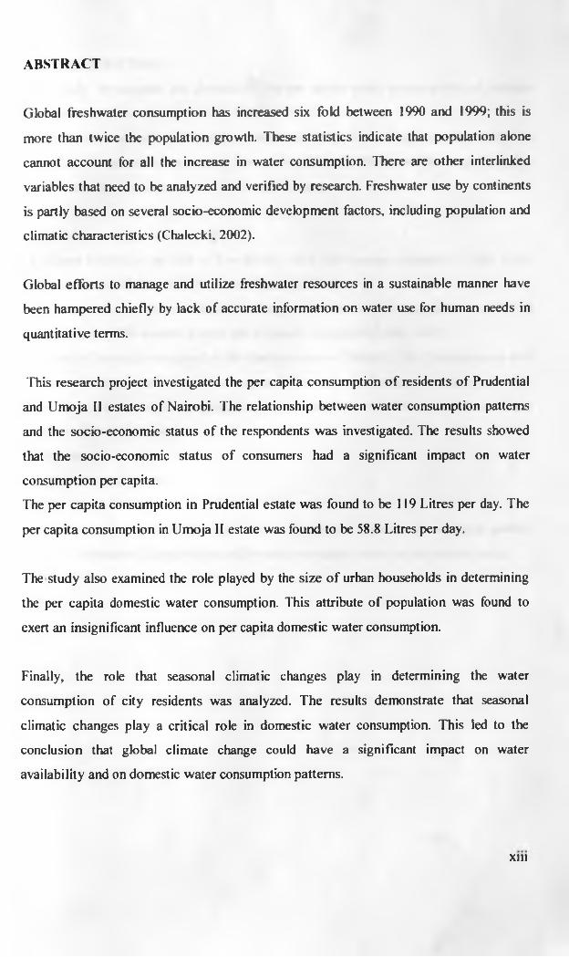
ABSTRACT

Global freshwater consumption has increased six fold between 1990 and 1999; this is

more than twice the population growth. These statistics indicate that population alone

cannot account for all the increase in water consumption. There are other interlinked

variables that need to be analyzed and verified by research. Freshwater use by continents

is partly based on several socio-economic development factors, including population and

climatic characteristics (Chalecki, 2002).

Global efforts to manage and utilize freshwater resources in a sustainable manner have

been hampered chiefly by lack of accurate information on water use for human needs in

quantitative terms.

This research project investigated the per capita consumption o f residents of Prudential

and Umoja II estates o f Nairobi. The relationship between water consumption patterns

and the socio-economic status of the respondents was investigated. The results showed

that the socio-economic status o f consumers had a significant impact on water

consumption per capita.

The per capita consumption in Prudential estate was found to be 119 Litres per day. The

per capita consumption in Umoja II estate was found to be 58.8 Litres per day.

The study also examined the role played by the size o f urban households in determining

the per capita domestic water consumption. This attribute of population was found to

exert an insignificant influence on per capita domestic water consumption.

Finally, the role that seasonal climatic changes play in determining the water

consumption of city residents was analyzed. The results demonstrate that seasonal

climatic changes play a critical role in domestic water consumption. This led to the

conclusion that global climate change could have a significant impact on water

availability and on domestic water consumption patterns.

Xlll

1.1 INTRODUCTION

This study investigated and determined the per capita water consumption of residents

from selected households in the city of Nairobi.

Primary data was obtained from the households selected to comprise samples for the

research. The source of secondary data was the Nairobi Water and Sewerage Company

water-metering depot situated at Kariobangi Estate.

Nairobi has been classified as follows:

A. Upper Nairobi is an area o f low density with high-income population, lying to the

West and North of the central business district (CBD).

B. Eastlands is the marginalized urban fringe to the East of and away from the CBD. It

has low and middle-income groups and is densely populated (Lillis, 1991).

The area o f research was based in the Eastlands area o f Nairobi. The Eastlands area falls

within the administrative region known as Embakasi constituency of Nairobi province.

This area has residential housing estates that indicate the different socio-economic

profiles o f the population.

Study sites

a) Prudential Estate,

b) Umoja II Estate.

Prudential estate represents the high-income population in this socio-economic profile.

Umoja II represents the population of low socio-economic status in this relative scale.

MAPS OF STUDY AREAS

MAP.A. LOCATION OF NAIROBI IN KENYA

Source: CIA world fact book-Kenya

2

MAP B. LOCATION OF EMBAKASI CONSTITUENCY IN NAIROBI

N denderuMtjfl.iqa ° Kamuqtiqa

Kiambu

Fmhakasi

Ttiigio

N achu

/ .iro b l Dannora

N a rob i Hi O

Kar«n

Ngonq

Marmbrti

?G0D MaoQjest com. Inc : & 2005 AND Products R V Source: www.mapqiiest.com

http://www.mapqiiest.com

MAP.C LOCATION OF PRUDENTIAL AND UMOJA II ESTATES IN

EMBAKASI CONSTITUENCY Scale. 1:20000

Source: www.hassconsult.co.ke

P *

http://www.hassconsult.co.ke

Photo I. A view of Prudential estate

Photo II. A view of Umoja II estateNote the water storage tank mounted on the rooftop.

5

1.2 BACKGROUND

Domestic water consumption in Kenya accounts for 20% of all water use. Agriculture

accounts for 76% while industrial use accounts for 4%. This distribution is common in

developing states, which rely heavily on agriculture. In most o f the developed states the

trends are reversed. For example Holland uses 34% of her water resources for

agriculture, 5% for domestic purposes, and 61% for industrial activities. On average, the

world uses 70% of fresh water for irrigation 20% for industrial purposes and 10% for

domestic use (Gleick et al, 2002).

In Kenya, the estimates of per capita water availability have been provided by various

sources with varying degrees o f accuracy and reliability.

According to the Kenya Ministry o f Water Resources Management and Development,

the country’s per capita water supply per annum stands at 647m3. This is projected to fall

to 235m3 by the year 2025 if the current state persists in terms of climate and population

growth. This estimate of 647 m3 is much higher than the World Resources Institute

(WR1) estimate made in 1990. The per capita water availability was 590m3 according to

the WRI. Critical areas of disagreement therefore occur in the estimates o f water resource

quantities as done by national agencies, United Nations bodies and professional groups.

Some o f the differences arise from periodical variations in precipitation experienced in

the country. On the global scene, data for small countries and countries in arid and semi

arid zones are less reliable than are those for larger and wetter countries.

The major area of agreement, however, is that water resource availability per capita is

likely to diminish in the future. There is also agreement among the scientific community

that per capita consumption is a reliable indicator o f water resource utilization. This

indicator allows for comparison with other countries. To make the comparison possible,

the sources o f data, the methods o f data collection, and the periods used for measurement

must be described in detail.

The methodology for determining per capita fresh water availability in a country relies on

population estimates and an estimate of the country’s internal renewable water resources.

The water resource available is then divided by the total population. The results are

given in cubic metres per capita per year. A similar methodological approach was

6

followed in this research. However, this research was mainly concerned with providing

precise figures on domestic water consumption per capita, and not estimates o f available

freshwater resources. The research was particularly focused on per capita water

consumption o f individuals in selected urban households.

Application of per capita measurement

Water consumption per capita is a widely used environmental indicator o f the state of

water resource use in any given geographical area. The per capita consumption is

developed from statistical parameters, but it has additional characteristics. It provides a

simpler and more readily understood form of information compared to complex data and

statistics. The per capita indicator has the potential o f reducing the uncertainty level

associated with decision making for environmental planning. The per capita

consumption is an indicator that relates environmental aspects to socio-economic factors.

In similar studies, the level o f consumption of water resources has been found to be

directly dependent upon the socio-economic status of the consumers (Postel. 1993)

7

1.3 THE PROBLEM STATEMENT

What is the per capita water consumption of residents in Nairobi households? This

research seeks to provide an answer to this question. The research problem is to

determine the current per capita domestic water consumption level.

Reliable information on the condition and trends in a country’s water resources in respect

o f quantity is required for such purposes as assessing the resources, and for determining

their potential for supplying the current and foreseeable demand.

Human population increase is related to increasing pressure on the water resource.

Nairobi has a growing water supply problem, which is linked to the original choice o f

site. The city was not originally planned to be a large densely populated urban area, and

the available water resources are only sufficient for a smaller population. To meet this

high and growing demand water has to be pumped from locations outside Nairobi.

Table 1.Population growth in Nairobi

Census Year Population

1969 509,256

1979 822,775

1989 1,600,000

1999 2,143,254

Source: republic o f Kenya, population and housing census reports.

Water scarcity is an ultimate constraint in the world's least developed countries (LDC’s)

development, and hence environmental and development issues must be considered

together. There is a sharp distinction between water capabilities in developed countries

and LDC’s. Many LDC’s happen to be located in the arid and semi arid tropics. About V*

o f the bottom 44 countries on the UNDP Human Development Index can be found in Sub

Saharan Africa

8

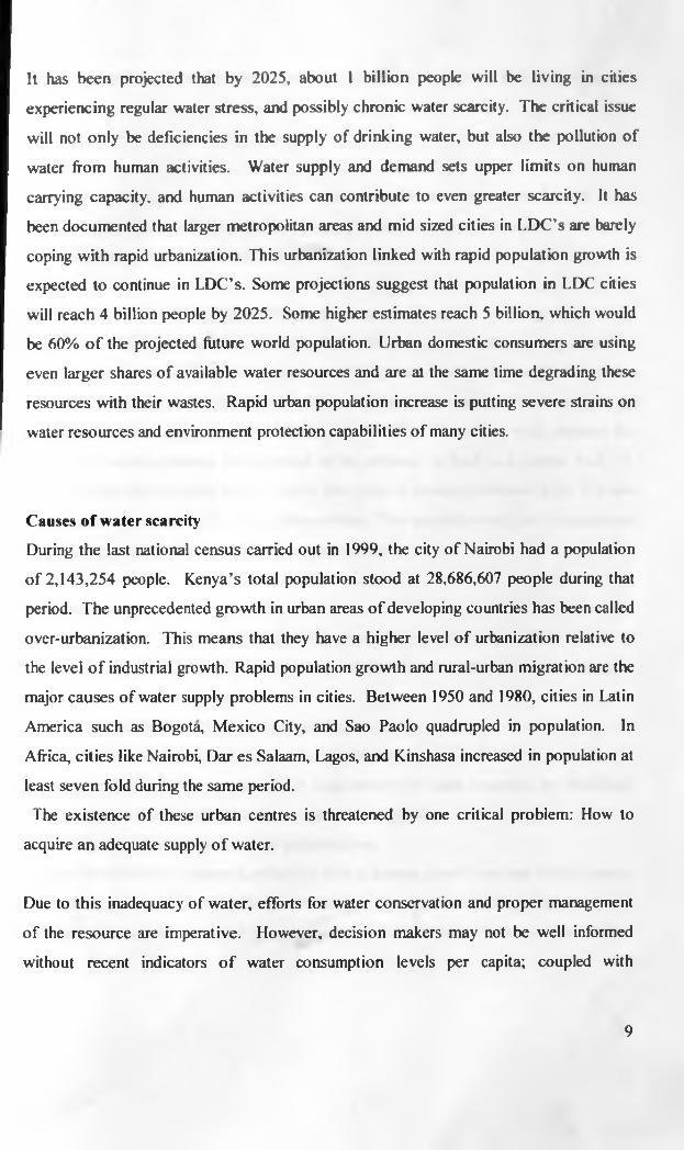
It has been projected that by 2025, about 1 billion people will be living in cities

experiencing regular water stress, and possibly chronic water scarcity. The critical issue

will not only be deficiencies in the supply of drinking water, but also the pollution o f

water from human activities. Water supply and demand sets upper limits on human

carrying capacity, and human activities can contribute to even greater scarcity. It has

been documented that larger metropolitan areas and mid sized cities in I.DC’s are barely

coping with rapid urbanization. This urbanization linked with rapid population growth is

expected to continue in LDC’s. Some projections suggest that population in LDC cities

will reach 4 billion people by 2025. Some higher estimates reach 5 billion, which would

be 60% o f the projected future world population. Urban domestic consumers are using

even larger shares o f available water resources and are at the same time degrading these

resources with their wastes. Rapid urban population increase is putting severe strains on

water resources and environment protection capabilities o f many cities.

Causes o f water scarcity

During the last national census carried out in 1999, the city o f Nairobi had a population

o f 2,143,254 people. Kenya’s total population stood at 28,686,607 people during that

period. The unprecedented growth in urban areas o f developing countries has been called

over-urbanization. This means that they have a higher level o f urbanization relative to

the level o f industrial growth. Rapid population growth and rural-urban migration are the

major causes o f water supply problems in cities. Between 1950 and 1980, cities in Latin

America such as Bogota, Mexico City, and Sao Paolo quadrupled in population. In

Africa, cities like Nairobi, Dar es Salaam, Lagos, and Kinshasa increased in population at

least seven fold during the same period.

The existence of these urban centres is threatened by one critical problem: How to

acquire an adequate supply o f water.

Due to this inadequacy of water, efforts for water conservation and proper management

o f the resource are imperative. However, decision makers may not be well informed

without recent indicators o f water consumption levels per capita; coupled with

9

knowledge o f the current numbers of the population, and their water consumption

patterns.

The main question is to what extent can water demand be met and under what

conditions; and how will the quality and quantity o f water be affected when the upper

limits of human population size are reached?

Despite the modem technology advancements, water demand in growing urban areas

cannot be indefinitely satisfied. Environmental damages are increasingly being caused by

the over exploitation o f freshwater sources. Urban growth is ultimately self-limiting, and

therefore urban planners and decision-makers must carefully consider how to make long-

range plans. These plans must be holistic, and should be in harmony with demands for

sustainable socio-economic development at the national, as well as a global level. A

determination o f the present water demand per capita o f urban populations is the first and

most logical step forward in solving this problem. This particular study is o f importance

as it seeks to provide answers to these very questions.

Knowledge gaps

The benefits and costs of providing a safe, convenient, and reliable water supply to

households in the developing world have been subject to vast and wide-ranging research.

Most o f this research has focused on:

a. The relationship between water and disease,

b. The efficacy o f water supply projects in improving health,

c. The causes and consequences o f rigid control o f water resources by individual

classes of society without the consideration o f gender,

d. The financing o f water supply infrastructure.

Despite this plethora o f research, relatively little is known about a number o f key aspects

o f domestic water use. In particular, knowledge is scarce about the long-term trends and

changes in household water use in any part of the world. This is because o f the lack of

10

quality baseline information and because of the cost and complexity o f undertaking

longitudinal and repeat studies.

Thus most research on household water use is limited to one season or year, or is carried

out within the narrow confines o f a donor-funded project or programme. Where studies

have attempted to examine changes over time, they have tended to be limited in scope,

frequently concentrating on a single locality, Coasequently, the dynamics and

determinants of domestic water consumption remain only partly understood. Among the

regions o f the world, these research gaps are most acute for sub-Saharan Africa, the

region whose population has the least access to improved water supplies (Thompson et

al, 2000).

11

1.4 RATION ALE/JUSTIFICATION OF THE PROBLEM

The U.N. programme of action (Agenda 21) proposes that countries should focus, inter

alia, on: a) Water and sustainable urban development,

b) Impacts o f climate change on water resources.

Scarcity o f fresh water resources and the escalating costs of developing new resources

have a considerable impact on all forms of national development and economic growth.

Urgent action is needed to improve the effectiveness o f the use o f water resources if their

contribution to human welfare and productivity is to be sustained. Special attention

needs to be given to the growing effects o f urbanization on water resource usage and to

the critical role played by local authorities and municipal authorities in managing the

supply, use and overall treatment o f water.

Better management o f urban water resources, including the elimination o f unsustainable

consumption patterns, can make a substantial contribution to the alleviation o f poverty

and improvement o f the health and quality o f life for the urban population.

Easy access to adequate water is a necessary condition for societal development, and

where water is scarce, human health and economic welfare suffer. These impacts o f

water scarcity are often more severe in urban areas with dense populations, such as

Nairobi’s Eastlands region.

In the early stages o f a nation’s development, the quantity of water is seen as the most

pertinent factor. In a country that is yet to industrialize such as Kenya, water quantity

management is of the utmost importance (UN-HABITAT, 2003).

This study hopes to produce accurate data concerning the water consumption patterns of

urban households in the study area. It is hoped that this data will enhance the discipline of

planning and management o f urban water resources.

12

1.5 ASSUMPTIONS AND VARIABLES

Per capita water consumption

The primary assumption in calculating the per capita water consumption is that each

household member has equal water needs. There is no distinction among the household

members on the basis of age, sex, race or body size. It is assumed that the water resource

is shared equitably within the household; hence total consumption per household is

divided by the number of individuals to derive the per capita consumption.

The calculation of per capita consumption over a prolonged period, such as consumption

per year or per month, is based on the assumption that there is no significant variation in

the day-by-day consumption patterns of the individuals. Any changes in consumption that

may arise from one day to the next are all reflected in the total consumption figure at the

end o f the period under investigation. On this basis, the total consumption per year may

be subdivided further to consumption per month, per week or per day according to the

objectives o f the researcher.

Variables

There are three important variables in domestic water consumption that are the subject of

this research. They are:

a) Household size,

b) Socio-economic status,

c) Seasonal climatic changes.

According to Ehrlich’s equation, Population, Affluence and Technology are critical

variables in determining people’s consumption o f natural resources .The equation is

expressed as follows:

I = P x A x T, where the impact on any natural resource is dependent on population,

affluence and technology factors. This formula has often been used to discuss the

connections between these variables. It has the appearance of a mathematical model that

may be revised to achieve greater precision as follows.

13

P-Population

The population dynamic that has been considered for investigation is the number o f

individuals per household. Much o f the debate on the impact of population on the

environment has been conducted in an unscientific manner. But things become clearer

when they are looked at quantitatively and in terms of physical mechanisms. Then

population tends to take its proper place as one of the key factors (Harrison, 1992).

The first assumption concerning population is that the greater the number o f individuals,

the greater their impact. Statistical methods are used to test this hypothesis in the course

this research. The data on household sizes and corresponding water consumption allows

for the quantitative analysis.

The second population assumption is that whenever common resources are shared within

a household setting, it leads to lower per capita consumption. This assumption is also

subjected to statistical investigation in this research project.

A-Affluence

It is the welfare status o f the population. It is assumed that the more affluent the

population, the more water they will consume for domestic purposes.

The poor often spend a higher percentage of their incomes on water than the affluent do

(UN-HABITAT, 2003). For purposes o f this research, the term affluence is replaced by

socio-economic status. This research investigates the impact of socio-economic status on

domestic water consumption.

T-Technology

This is the technological choice o f the population. In this research, the technology used

to obtain water is the same for all the samples. They are using piped water, which is

distributed directly to the respective households by the Nairobi Water and Sewerage

Company. The Company measures the volume o f water consumed by each household.

The rates are based on a volumetric charging system. The pricing rates o f water are the

same for all the households sampled in this research.

14

1.6 AIMS AND OBJECTIVES

The aim o f this research project is to determine the per capita water consumption o f

selected Nairobi households. The study set out to generate new data concerning the

water consumption patterns o f these households. This information will be useful as a tool

for policy formulation and in supporting the management decisions of planners and other

stakeholders in the Kenyan water sector. It is hoped that the results from this research

will also provide baseline data that may enhance further research possibilities on the

Kenyan freshwater resources. For example, similar research may be done periodically to

establish the trends in water consumption in the research areas.

In this way, it is hoped that the research will contribute towards sustainable water

resource management in urban areas of Kenya.

Objectives

1) To compute the correlation between household size and per capita water

consumption.

2) To investigate the impact o f socio-economic status on per capita domestic water

consumption.

3) To examine the impact o f climatic variations on domestic water consumption per

capita.

15

1.7 HYPOTHESES

1) H„ The household size has no significant impact on the per capita water

consumption.

H | The household size has a significant impact on the per capita water consumption.

2) H0 The socio-economic status of consumers has no significant impact on per capita

water consumption.

Hi The Socio-economic status of consumers has a significant impact on per capita

water consumption.

3) H0 Climatic variations have no significant impact on domestic water consumption.

H | Climatic variations have a significant impact on domestic water consumption.

16

2.0 LITERATURE REVIEW

2.EWORLD WATER

Table.2 The Distribution of Water across the Globe

^ocation Volume

(103km3)

Total Vol. in

Hydrosphere

-ere (%)

Fresh water

(%)

Annual Vol.

recycled in

km3

Renewal

period years

i>cean 1,338,000 96.5 - 505,000 2,500

groundwater (gravity

capillary)

23,400* 1.7 16,700 1,400

f* redominantly fresh

t round water

10,530 0.76 30.1

;>oil moisture 16.5 0.001 0.05 16,500 1

Zjlaciers & permanent

»now cover

24,064 1.74 68.7

LJround ice

Permafrost)

300 0.022 0.86 30 10,000

W ater in lakes (Total) 176.4 0.013 - 10,376 17

resh water lakes 91.0 0.007 0.26 - -

Salt water lakes 85.4 0.006 - - -

Vlarshes & swamps 11.5 0.0008 0.03 2,294 5

River water 2.12 0.0002 0.006 43,000 16 days

biological water 1.12 0.0001 0.003 - -

W ater in atmosphere 12.9 0.001 0.04 600,000 8 days

ro ta l V. in hydrosphere 1,386,000 100 - - -

I'otal freshwater 35,029.2 2.53 100% - -

^Excluding groundwater in the Antarctic, estimated at 2,000,000 km3 and including

predominantly freshwater o f 1,000,000 km3 (UNESCO, 2003).

17

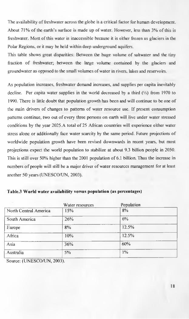
The availability of freshwater across the globe is a critical factor for human development.

About 71% o f the earth’s surface is made up of water. However, less than 3% o f this is

freshwater. Most of this water is inaccessible because it is either frozen as glaciers in the

Polar Regions, or it may be held within deep underground aquifers.

This table shows great disparities: Between the huge volume o f saltwater and the tiny

fraction o f freshwater; between the large volume contained by the glaciers and

groundwater as opposed to the small volumes of water in rivers, lakes and reservoirs.

As population increases, freshwater demand increases, and supplies per capita inevitably

decline. Per capita water supplies in the world decreased by a third (Vi) from 1970 to

1990. There is little doubt that population growth has been and will continue to be one o f

the main drivers of changes to patterns o f water resource use. If present consumption

patterns continue, two out of every three persons on earth will live under water stressed

conditions by the year 2025.A total of 25 African countries will experience either water

stress alone or additionally face water scarcity by the same period. Future projections o f

worldwide population growth have been revised downwards in recent years, but most

projections expect the world population to stabilize at about 9.3 billion people in 2050.

This is still over 50% higher than the 2001 population of 6.1 billion. Thus the increase in

numbers o f people will still be a major driver of water resources management for at least

another 50 years (UNESCO/UN, 2003).

Table.3 World water availability versus population (as percentages)

Water resources____________ PopulationNorth Central America 15% 8%

South America 26% 6%

Europe 8% 12.5%

Africa 10% 12.5%

Asia 36% 60%

. Australia 5% 1%

Source: (UNESCO/UN, 2003).

18

The global overview o f water availability versus the population stresses the continental

disparity. Asia supports more than half the world population with only 36% of the

world's freshwater resources.

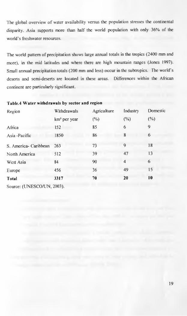
The world pattern of precipitation shows large annual totals in the tropics (2400 mm and

more), in the mid latitudes and where there are high mountain ranges (Jones 1997).

Small annual precipitation totals (200 mm and less) occur in the subtropics. The world's

deserts and semi-deserts are located in these areas. Differences within the African

continent are particularly significant.

Table.4 Water withdrawals by sector and region

Region Withdrawals

km3 per year

Agriculture

(%)

Industry

(%)

Domestic

(%)

Africa 152 85 6 9

Asia -Pacific 1850 86 8 6

S. America- Caribbean 263 73 9 18

North America 512 39 47 13

West Asia 84 90 4 6

Europe 456 36 49 15

Total 3317 70 20 10

Source: (UNESCO/UN, 2003).

19

2.2 AFRICA

The African continent occupies an area of 30.1 million km’ . It has a rapidly growing

human population that is well over 700 million, many living in the world’s least

developed countries.

During the decade from 1990 to 2000, Africa suffered a third of the world's water related

disaster events (floods and droughts), with nearly 135 million people affected. About

80% of these are affected by drought and the unavailability o f water. Moreover, the

increasing frequency o f floods and droughts will exert greater pressure on freshwater

ecosystems and on the freshwater provision networks and infrastructure. All the above

factors will act together to pose enormous difficulties in the storage, provision and

distribution o f water, as well as water treatment (water purity and purification o f used

water).

Freshwater availability in Africa

The availability of freshwater in Africa is one o f the most critical factors governing

development in the continent. The mean water availability per capita in Africa is about

5,720 cubic metres per year. This is lower than the global average of 7,600 cubic metres

per capita per year. There are, however, large disparities in the world's sub-regions.

The intergovernmental group o f experts on climate change anticipates a decline in stream

flows and mean availability o f freshwater in African countries, mainly in the North and

South. These changes are expected to impact the freshwater ecosystems negatively.

Access to freshwater resources

Major difficulties of water provision have been observed in countries that have less than

1700 m’ per capita per year. Water stress o f less than 1000 nr per capita per year has

been observed in 14 o f 53 African countries with available data.

The access to water resources is therefore a priority question for African countries,

together with concerns over decreasing water quality due to excessive withdrawals, the

declines in reservoirs and pollution from various sources. Due to these circumstances, 25

African countries will experience either water stress or water scarcity, and difficulties in

water supply within the 2020 to 2030 decade (UNEP, 2002).

20

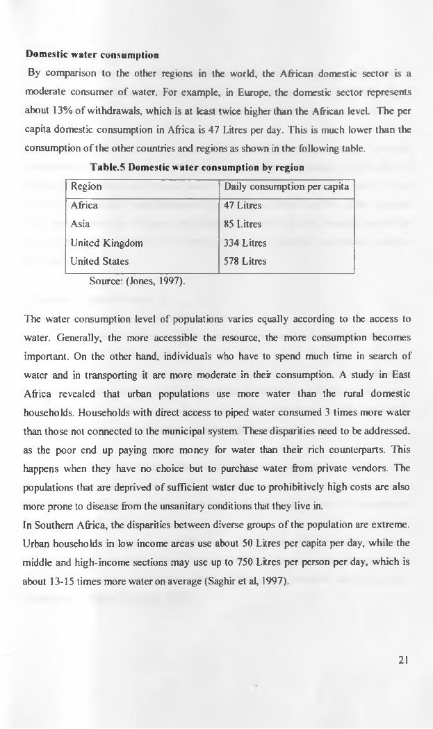
Domestic water consumption

By comparison to the other regions in the world, the African domestic sector is a

moderate consumer o f water. For example, in Europe, the domestic sector represents

about 13% of withdrawals, which is at least twice higher than the African level. The per

capita domestic consumption in Africa is 47 Litres per day. This is much lower than the

consumption of the other countries and regions as shown in the following table.

Table.5 Domestic water consumption by region

Region Daily consumption per capita

Africa 47 Litres

Asia 85 Litres

United Kingdom 334 Litres

United States 578 Litres

Source: (Jones, 1997).

The water consumption level of populations varies equally according to the access to

water. Generally, the more accessible the resource, the more consumption becomes

important. On the other hand, individuals who have to spend much time in search of

water and in transporting it are more moderate in their consumption. A study in East

Africa revealed that urban populations use more water than the rural domestic

households. Households with direct access to piped water consumed 3 times more water

than those not connected to the municipal system. These disparities need to be addressed,

as the poor end up paying more money for water than their rich counterparts. This

happens when they have no choice but to purchase water from private vendors. The

populations that are deprived of sufficient water due to prohibitively high costs are also

more prone to disease from the unsanitary conditions that they live in.

In Southern Africa, the disparities between diverse groups o f the population are extreme.

Urban households in low income areas use about 50 Litres per capita per day, while the

middle and high-income sections may use up to 750 Litres per person per day, which is

about 13-15 times more water on average (Saghir et al, 1997).

21

2.3 KENYA

The republic o f Kenya is positioned across the equator, and has geographical diversity in

terms of climate, physiography and geology. It has a surface area o f 583,000 km2 , of

which 569,000 km2 is land surface while the remaining 14,000 km2 portion is water.

Most rains occur from May to August. Months with the highest rates o f potential

evapotranspiration are the ones with least rainfall. The geographical distribution of

surface water resources in Kenya is varied. Severe droughts occur in more than % of the

country, one in every 5 years because o f failure o f rains. More than 63% of the total area

of Kenya receives only 500 mm rainfall per year. However, the well-watered parts o f the

country support nearly 80% of the population through agriculture and related activities

(Khroda. 1988).

Drainage systems of Kenya

There are three major drainage systems in Kenya.

The Nile basin system. This drains the western flank o f the Rift valley into

the Mediterranean Sea.

- The internal drainage, which comprise the great Rift valley with many

lakes and rivers draining into them. Chalbi desert and the lake Amboseli.

- The Indian Ocean drainage system. This includes rivers Athi, Tana, Voi,

Ewaso Ngiro (North) and other smaller streams.

The characteristics o f the Kenya rivers are adduced from the annual distribution o f the

river run-off (stream flow). The typical feature o f the duration period o f the surface run

off (flood) of the Kenya rivers dominating most o f the territory is about 2-3 months and

8-9 moths in the South-western Kenya.

Some o f the major perennial rivers in Kenya are Tana, Nzoia, Athi, Sondu, Ewaso Ngiro

(North), Ewaso Ngiro (South), Yala. Nyando and Mara. However, water shortage is one

o f the features covering the greater territory o f the country, with the exception o f the

South-western Kenya (Ogembo, 1980).

22

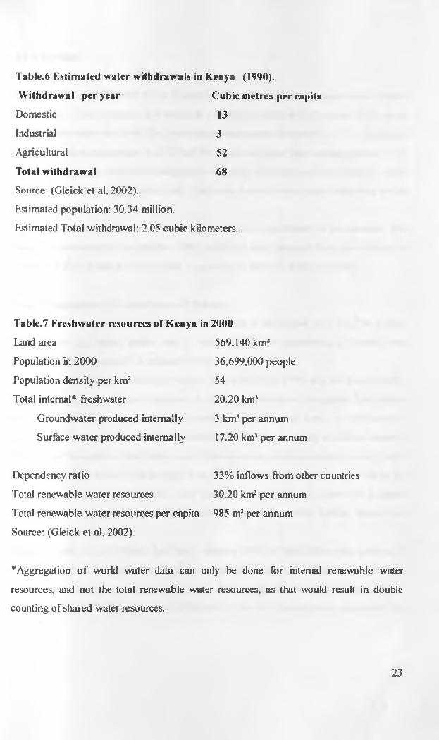
Table.6 Estimated water withdrawals in Kenya (1990).

Withdrawal per year Cubic metres per capita

Domestic 13

Industrial 3

Agricultural 52

Total withdrawal 68

Source: (Gleick et al, 2002).

Estimated population: 30.34 million.

Estimated Total withdrawal: 2.05 cubic kilometers.

Table.7 Freshwater resources of Kenya

Land area

Population in 2000

Population density per km2

Total internal* freshwater

Groundwater produced internally

Surface water produced internally

in 2000

569.140 km2

36,699,000 people

54

20.20 km3

3 km3 per annum

17.20 km3 per annum

Dependency ratio

Total renewable water resources

Total renewable water resources per capita

Source: (Gleick et al, 2002).

33% inflows from other countries

30.20 km3 per annum

985 m3 per annum

*Aggregation o f world water data can only be done for internal renewable water

resources, and not the total renewable water resources, as that would result in double

counting of shared water resources.

23

2.4 NAIROBI

Climatic characteristics of Nairobi

The city of Nairobi is about 40 km South of the Equator, but the temperatures are altitude

- modified. This is because it is found at a fairly high altitude, of between 1650 up to

1800 metres above sea level. The mean annual temperature in the city is 17°C. The mean

daily maximum temperature is 23°C and the mean minimum daily temperature is 12°C.

The month o f mean maximum temperature is usually February, and the month o f mean

minimum temperatures is usually July. The mean monthly evaporation rates vary as the

mean monthly temperatures vary.

The mean annual rainfall is 1,080 mm. This rainfall is experienced in two seasons. The

long rains are usually from March to May, while the short rains are from mid-October to

December. Fifty percent o f the rainfall is experienced between March and May.

Human population Characteristics of Nairobi

Nairobi is the capital city o f Kenya. The city had a population o f 2,143,254 people

according to the census carried out in August 1999. The population in Nairobi was

estimated to have reached 2.5 million in 2003.

The total number o f households in Nairobi was 649,426 in 1999, and the mean density

was 3,079 people per square kilometre. A closer examination o f the spatial distribution

reveals that there are areas of low-density population and areas of high-density

population. The majority o f Nairobi residents occupy the high-density residential areas to

the East and Northeast of the Central area. There are some medium -density housing units

to the North and West of the Central area. The low-density residential units are to be

found in the extreme Northwest, and include Karen and some parts o f Langata

constituency. A sprawling area o f informal settlements called Kibera slums has

developed within Langata.

Eighty percent o f the Nairobi land area supports 20% o f the high-income groups in

suburban planned residential developments. The low-income group, constituting 80% of

the population, are sprawled in the remaining 20% residential land, contributing to high

population density and water supply difficulties. These low-income areas experience the

24

highest rate o f population growth due to rural-urban migration and natural increase

(Khroda, 1988).

Water demand in Nairobi

In Nairobi, the total demand for water in 1990 was about 50 million cubic metres per

year. The Tana and Athi Rivers have met much of this need. The Tana supplied 81%

while Athi River supplied 19% o f the water (40.5 million cubic metres and 9.5 million

cubic metres per year respectively). When rainfall is inadequate, some parts o f Nairobi

City face water shortages and the normal production is disrupted. In the year 2000, this

was the scenario at Nairobi’s water sources.

Table.8 Nairobi water demand and supply in 2000

Source Normal production capacity Supply in 2000

mJ/day mVday Shortfall per day

Kikuyu springs 4,000 4,000 Nil

Ruiru dam 12,000 11,700 300

Sasumua dam 40,850 19,200 21,650

Ngethu/Thika Dam 289,750 240,000 49,750

Total 346,600 274,900 71,700

Source: (Makuro, 2000).

Some changes are evident in the ten-year period between 1990 and 2000. From a demand

of 50 million cubic metres a year, the demand in 2000 had increased to about 126 million

cubic metres per year. This is about 2.5 times increase in demand over a ten-year period.

The drought conditions in 2000 had a severe impact on the water supply situation.

Among the factors cited as key to this shortfall in supply was destruction of forests and

degradation o f water catchment areas, leading to changed hydrologic conditions and

adverse weather patterns. Consequently this degradation leads to increased runoffs that

are short-lived, with resultant siltation problems in dams and intakes. The concept is that

the management o f land and its cover affects the water quantity, duration of river flows

and amount of sediment contained in the water (Tebbutt, 1990).

25

2.5 THEORETICAL FRAMEWORK

Freshwater-population interaction

It is important to analyze demographic features in Africa in order to help demonstrate

their interaction with freshwater resources, systems and management. As a monolithic

concept, ‘population’ in relation to physical and socio-economic phenomena remains

vague, and its popularly advocated effects and how it is affected by these phenomena

lacks strong empirical evidence. In Africa, what should concern the scientific community

is how much research, if any, has explored the freshwater- population dynamics

relationship.

The concept o f ‘population dynamics’ relates strictly to the three components of

population, namely: fertility, mortality and migration, which determine the population

change and structure. Population change in urban areas is due to both natural increase

and migration. The natural increase is simplified as births minus deaths within the

population. ‘Population structure’, on the other hand, denotes innate attributes o f the

population such as gender and age. The population structure also denotes the acquired

socio-economic attributes such as economic activity, educational attainment, language

group and marital status. Freshwater management must take cognizance of community

population dynamics, the primary factor being household size (Oucho, 2001).

The following three issues help to illustrate some pertinent aspects o f the freshwater -

population dynamics.

1) Freshwater resources and withdrawals.

2) Population and annual renewable freshwater availability in the past, present and

. future years.

3) The proportion o f population without access to safe water.

Freshwater resources and withdrawals

There are three features of freshwater resources and withdrawals that are listed below as:

i) Annual river flows

ii) Annual withdrawals

iii) Withdrawals by different sectors (domestic, agricultural and industrial sectors).

These features deserve analysis and research (UNEP/HABITAT, 1999).

26

Huge capital and recurrent expenses are needed particularly to meet energy, chemical

and labour requirements o f urban water schemes. The planner’s task is, therefore, to

determine what should be the optimum size o f a water supply scheme within some

financial and environmental constraints (So et al, 1982). The ultimate capacity o f a water

supply scheme is usually considered in relation to three crucial variables.

These are:

- The ultimate extent o f the service area,

- The ultimate service population, and

The projected per capita water consumption per unit time (Iteke, 1980).

It is thus not practical for a water supply system to strive to meet the demand o f an ever-

expanding population spread over an unlimited service area. It is also unreasonable to

expect a water supply system to meet unrestricted demand per capita per unit time. It

becomes apparent that the planning for city water resources cannot be successful without

the availability o f regularly updated per capita water consumption data

Water stress

Unlike water quality standards for which there are accepted guidelines and specific

targets, there are no universally agreed standards that have been established for water

quantity. As such, there is no precise universal minimum daily water allowance or

requirement per capita stipulated by the W.H.O or any other international body. At the

second world water forum and inter-ministerial meeting held in March 2000 in the

Netherlands, there was a failure to address this issue of quantity. The amount available

per capita for most cities in developing states frequently remains well below the

minimum standards suggested by national governments and international bodies.

Although 20 litres per person per day is currently the standard for household water

consumption, it has been estimated that 30 to 40 Litres a day are the minimum needed per

person if drinking, cooking, laundry and basic hygiene are all taken into consideration

(Thompson et al, 2000).

27

It is possible to make a quantitative comparison between a country’s water availability

per capita to the per capita demand. Once the per capita demand has been established,

mathematical projections may be made for a future situation where a better quality o f life

has been attained. Such projections are based on the observation that economic

development is often accompanied by increased water consumption per capita. The

population changes must also be taken into account. This, however, is only possible in

countries that have the relevant water consumption statistics (Shiklomanov, 1993).

Economic development and natural resource consumption.

Various researchers have described the connection between economic development and

the consumption of natural resources. In our focus on the natural resource of freshwater,

the economic system is dealt with insofar as it generates both the demand and the means

for freshwater resource exploitation (de Vries et al, 1997).

The increasing pressure on the regional and global freshwater environment is caused not

only by the growing population, but also by the ever-large thoroughput of materials

associated with the life-styles o f more affluent regions. These larger thoroughputs are

directly associated with increasing human welfare, in the form o f dwellings and

household activities. It has become evident that they cause various undesirable side

effects, among which is environmental degradation and natural resource depletion. Such

externalities, as they are called in economic literature, tend to offset part of the gains in

welfare. However, both welfare and the perceived loss o f welfare through environmental

degradation are difficult, or even impossible to quantify in unambiguous and non-

controversial terms (Rotmans et al, 1995).

For these reasons, population and economic development are related to the rate of

consumption o f freshwater resource in the conceptual framework o f this project.

Economic development is a strong factor in domestic water consumption. The UNDP

Human Development Report (1998) highlights disparities in freshwater use based not on

accessibility, but on economic development. The report found that a new bom baby in the

28

North could consume 40-70 times more water than a new bom baby in the South who has

equal access to water. It is therefore critical to examine the roles of population size and

economic development in a conceptual framework that establishes their respective

impacts on domestic freshwater consumption. The impact o f climatic conditions on water

consumption patterns must also be investigated in the same framework.

29

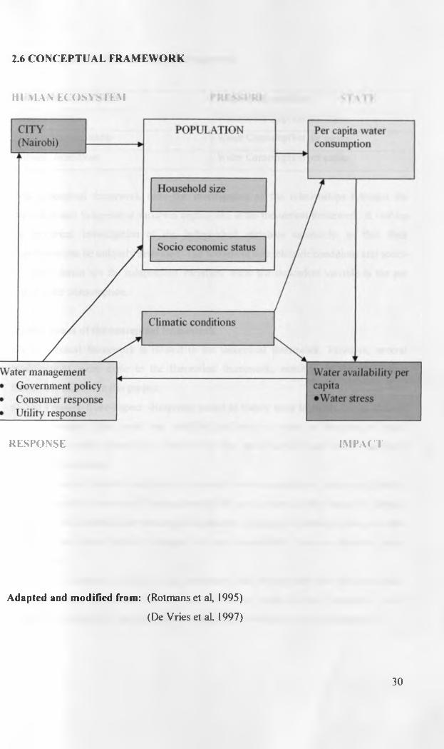
2.6 CONCEPTUAL FRAMEWORK

HUMAN ECOSYSTEM

RESPONSE IMPACT

Adapted and modified from: (Rotmans et al, 1995)

(De Vries et al. 1997)

30

Table.9 Variables in the conceptual framework

Independent variables Dependent variable

Household size Water Consumption per capita

Socio-economic status Water Consumption per capita

Climatic conditions Water Consumption per capita

This conceptual framework suits the investigation o f the relationships between the

dependent and independent variables highlighted in the theoretical framework. It enables

the empirical investigation of the independent variables separately, so that their

importance can be uniquely described The household size, climatic conditions and socio

economic status are the independent variables, while the dependent variable is the per

capita water consumption.

Modifications of the conceptual framework

The conceptual framework is related to the theoretical framework. However, several

modifications were made to the theoretical framework, resulting in the conceptual

framework utilized in this project.

a) The Pressure-State-Impact -Response model is widely used to report on the state of

the environment. This model was modified and used to report on the state o f water

consumption within households. That is the first modification made in this project’s

conceptual framework.

b) The impact o f climatic conditions on domestic water consumption was a modification

o f the conceptual framework. Previous models did not account for this impact o f climatic

conditions on domestic water consumption patterns. According to earlier models, climatic

conditions are better known to impact on water availability than on domestic water

consumption.

c) The socio-economic status of water consumers was incorporated into this conceptual

framework. The importance of the socio-economic status is that prosperity levels

provide the demand for, and means o f sustaining high domestic water consumption.

31

2.7 LIMITATIONS OF THE STUDY

The study is limited to the middle-income and high-income groups within the Eastlands

area o f Nairobi. The study does not cover the low-income groups that reside in informal

settlements because they lack individual water meters in their households.

Delimitations of the study

The computed results concerning the correlation between household size and per capita

water consumption may safely be generalized to comparable urban households with

piped water supplies.

The results on the impact of socio-economic status on per capita water consumption

may safely be generalized to comparable urban households that have the same water

tariffs, and the same level o f service from the water utility.

The findings on the impact of climatic conditions on domestic water consumption may

safely be generalized to comparable urban households.

32

2.8 DEFINITION OF TERMS

Per capita: The term per capita literally means per person. This is regardless o f the age

and gender o f the person.

The per capita water consumption is expressed as litres consumed per person per day

(1/p/d).

Per capita consumption may be calculated per day, per month or per year, and these

different time periods were specified in this research where necessary.

The units o f water consumption are in cubic metres (m3 ). 1 m3 is equivalent to 1000

litres o f water.

Household size: The total number o f individuals being served by a single water meter in

a household constitutes the household size. ‘Piped’ households are those with access to

direct and functional water connections within the house or immediate compound. A

functional piped system is one from which a household could satisfy its basic water needs

throughout the year.

Domestic water consumption: This refers to the total and combined amount o f water

that is used for drinking, cooking, washing and sanitation in the house. It also includes

water used in watering plants in household gardens.

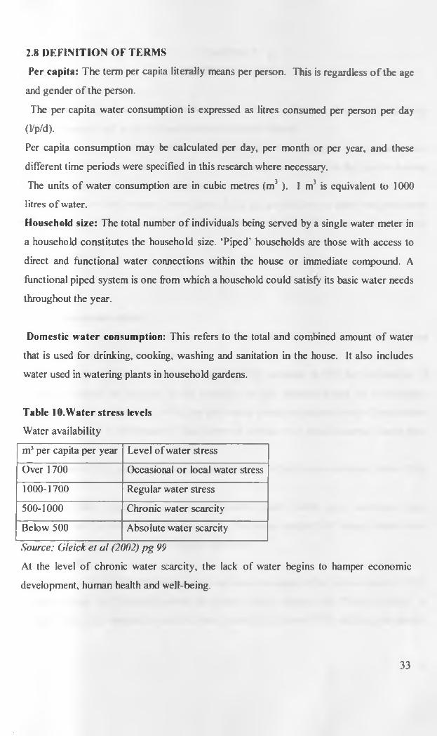
Table 10.Water stress levels

Water availability

m3 per capita per year Level of water stress

Over 1700 Occasional or local water stress

1000-1700 Regular water stress

500-1000 Chronic water scarcity

Below 500 Absolute water scarcity

Source: Gleick ei al (2002) pg 99

At the level o f chronic water scarcity, the lack o f water begins to hamper economic

development, human health and well-being.

33

CHAPTER 3

METHODOLOGY

3.1 Introduction

In this research project, Nairobi is defined as the universe o f interest. Prudential and Umoja

II estates are defined as two distinct populations within Nairobi

Prudential estate is a homogeneous population based on the type o f housing and water

facilities. By the same token Umoja II estate is homogeneous based on the type o f housing

and water facilities available to the population.

The samples for this research were drawn from the populations in these two residential

estates. The main distinction between the two estates was the difference in socio-economic

status

3.2 Socio-economic status

There are various indicators of socio-economic status. These include income levels, type and

location of housing, and house rent.

People are often elusive to questions concerning their incomes. It calls for the exercise of

dictatorial powers on the part of the researcher to get accurate details on respondent’s

incomes (Boreham & Semple, 1976) For this reason, details on income levels o f respondents

were not required in this research. The following indicators o f socio-economic status were

used instead.

a) The location and quality o f urban housing tends to reflect socio- economic status (Peil,

1983)

Prudential estate consists o f spacious maisonettes, each having four bedrooms. Each

maisonette has a servant's quarter and a lawn. The houses sampled in Umoja II estate were

less spacious, and each house had a single bedroom.

b) House rent

The house rent required for the houses was used as an indicator o f the socio-economic status

o f the residents. In Prudential estate, the house rent per month was 25,000 shillings. In

Umoja II estate the households sampled were rented at the sum o f 5,000 shillings per month.

34

From the house rents, it was clear that Prudential estate represents the population o f high

socio-economic status. Umoja II estate represents the population o f low socio-economic

status in this comparative scheme.

Photo III. Houses in Prudential estate

Photo IV. A Street and houses in Unioja II estate

3.3 Prudential estate

First a letter was written to the security chairman of Prudential estate stating the intent to

conduct research in the estate. Unfortunately, this was the period in which some University

o f Nairobi students had been involved in armed robberies and a cache o f weapons had been

u n i v t s ?EAS ' A - ,

, TY O F N A I R O B ICANA COLLECTION

35

' ■ f V Y A T T * o£,''.'~ , P3,AL, jm fQ

found in the University's Mamlaka hostels. Due to this negative publicity, the Prudential

Estate security chairman gave strict conditions. The researcher was not allowed to personally

enter into any o f the households, but was to conduct investigations from outside the gates.

For this reason, questionnaires were used in Prudential estate. The questionnaires were

issued to the respondents under the supervision o f the security personnel o f Prudential estate.

3.3 a) Sampling methodology in Prudential Estate

Prudential estate has a total of 88 house units. However, the total number o f residential

houses was only 74 at the time o f this research. This is because some of the units were

unoccupied at the time o f research, while other units were used for commercial purposes.

Some examples o f commercial purposes were a pre-school, Prudential farmers co-operative

society offices, and a shopping centre within the estate. Due to the presence o f residential

and non-residential units, stratified sampling was done. One stratum was made up o f the 14

non-residential houses, and the other stratum comprised the residential units. Only the 74

residential units formed the target population.

Photo V. A house in Prudential estate

A preliminary or test questionnaire was formulated and issued to 30 households. Their

responses would indicate whether the questionnaire had been well formulated. After

36

receiving the responses, the questionnaire was modified to make it easy to use, and to

capture the precise information required. It was also discovered that the residents preferred a

questionnaire giving them a deadline as to when the researcher would collect the results. In

this regard the final questionnaire stipulated the exact time when the questionnaires would be

collected. This would facilitate the quick collection of data and ensure a high percentage of

returned questionnaires.

The modified questionnaires were then issued to all the 74 residential households in

Prudential estate. Thus the entire target population was issued with questionnaires. A period

o f one week was given as the deadline for the collection o f all the questionnaires, but it was

later extended to the second week. The issuance and collection o f questionnaires was done in

the early evening during the weekends. At the end o f this period, a total o f 37 duly

completed questionnaires were recovered. One questionnaire among the 37 was disregarded

because the occupant had moved into the estate only two months prior to the research. It is

only the respondents who had lived in the same house, for more than one year prior to the

research that could give the required information. This is because their water consumption

during the previous one-year was the subject of investigation.

3.3 b) Data evaluation

The consumption data for each household was obtained from the meter readings at the

Nairobi Water and Sewerage Company depot at Kariobangi. The meter readings consist the

raw data that the utility uses to produce consumer water bills.

First the House numbers in the questionnaires were matched with the utility’s meter card

readings. There was no inconsistency between the house numbers as given by the

respondents and the ones in the meter cards. The meter card that has Prudential estate data is

number ‘37-16’. The figure ‘37’ represents the area number, while ‘16’ is the specific meter

card for Prudential estate.

However, there were various reasons that led to the disuse o f some questionnaires. The main

reasons why some households were not included in the final sample for research were as

follows.

37

• Inconsistent meter readings and estimates.

Data from houses that had inconsistent meter readings and estimated water consumption

readings were not processed any further. The meter readers marked the initials (Ikd) in some

of the meter cards, and these initials indicated the houses that were locked at the time of

meter reading. All such houses were eliminated from the sample because accurate meter

readings are imperative for water consumption research.

Photo VI. Position of water meter within a compound in Prudential estate

Note. The blue water meter is nearly overgrown with weeds. The meter is inaccessible to

meter readers when the gate is locked.

• Spoilt meters

Any households that had spoilt water meters at any time during the year under investigation

were removed from the sample. The initials in the meter readings at the depot were marked

(m/s) to indicate spoilt meters. Consequently, all houses that had their water meters replaced

during the period o f interest were not included in the final sample o f prudential estate.

After these processes o f data evaluation, the total sample in Prudential estate was reduced to

29 households out o f a total o f 37 households that initially had returned the questionnaires.

The final sample size from Prudential estate was 39 % of the total population. This sample

size was representative of the population in Prudential estate.

38

3.4 Umoja II estate.

Umoja II estate was stratified on the basis o f residential and non-resident ial houses. The

owners had converted some of the houses into business premises. The most common

commercial uses were retail shops, beauty salons, food kiosks, butcheries, grocery shops,

video arcades, medical clinics and laboratories; tailoring shops, clothing stores,

communications bureaus, bars, churches and hardware stores. All o f these non-resident ial

houses were not part of the sample. It is only the stratum consisting of residential houses

that was sampled for research

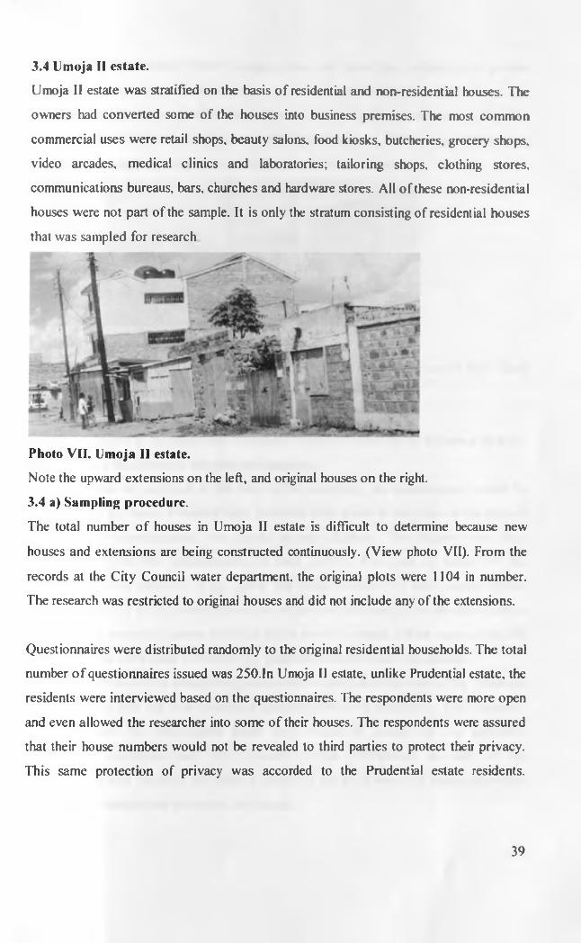
Photo VII. Umoja II estate.

Note the upward extensions on the left, and original houses on the right.

3.4 a) Sampling procedure.

The total number o f houses in Umoja II estate is difficult to determine because new

houses and extensions are being constructed continuously. (View photo VII). From the

records at the City Council water department, the original plots were 1104 in number.

The research was restricted to original houses and did not include any of the extensions.

Questionnaires were distributed randomly to the original residential households. The total

number o f questionnaires issued was 250.1n Umoja II estate, unlike Prudential estate, the

residents were interviewed based on the questionnaires. The respondents were more open

and even allowed the researcher into some o f their houses. The respondents were assured

that their house numbers would not be revealed to third parties to protect their privacy.

This same protection of privacy was accorded to the Prudential estate residents.

39

Furthermore, the Nairobi Water Company does not allow the publication o f private

account details o f water consumers.

The areas that were surveyed in Umoja II were area ‘31’, (meter cards 9 and 10). The

other area was ‘32’, (meter cards 18 and 19). The terms area ‘31’ and area ‘32’ refer to

administrative regions as demarcated by the Nairobi Water Company.

Photo VIII. Original Umoja II houses.

Samples were drawn from original houses only. Note the school gate on the right. Such

non-residential houses were not part o f the sample

Random sampling o f the residential households was determined by the following factors,

a) Presence in the house at the time o f sampling.

If a house had no occupant at the time of the sampling, the questionnaire would be

slipped under the door. Whenever only juveniles were found in the house at the time of

sampling, the questionnaires were given to such children. The children were duly

instructed to give the questionnaires to their parents. The time o f return for the

questionnaire was indicated in the form. The house numbers o f each sampled house

were recorded in a field notebook as well as on the questionnaires .If on the day of return

the occupants were still unseen, then that house would be struck off the samples list. No

further attempts were made to recover the questionnaires from such households.

In some o f the houses the completed questionnaires were found upon returning. Some of

the respondents also left their completed questionnaires with neighbours. This happened

in cases where the respondents knew they would be absent on the appointed

questionnaire collection day. The accuracy of the information on each o f the

questionnaires was checked, and upon satisfaction, the form was filed among the other

usable questionnaires that comprised the sample.

40

b) Willingness to be interviewed

Some respondents preferred to answer the questionnaire with the help o f the researcher

and their wishes were obliged. Some o f the respondents preferred to fill the forms

themselves and they were free to do so. In some houses, the residents were unwilling to

be interviewed based on the questionnaires and disqualified themselves from

participation in the research. Their wishes were also granted. It emerged that friends and

neighbours had a big influence on each other. In any plot where the first person met was

willing to participate, the rest o f the neighbours were more likely to participate.

Whenever the first person approached turned away the researcher and suggested he

interviews the neighbours instead, the other neighbours were equally unwilling to

participate in the research.

The refusal to be interviewed or to fill the questionnaire was one o f the problems

encountered. Some o f the respondents were also afraid that they could be incriminating

themselves by giving the research information, and they had to be reassured that their

names and house numbers would not be published. Upon such reassurance, many

respondents then became willing to participate in the research.

c) Period of residence in the same house

Some o f the questionnaires were discarded even after they were properly filled whenever

it emerged that the respondents had not lived in their current house for a period o f at least

one year. It was apparent that in Umoja II estate there were more frequent cases of

movement from other houses than in Prudential estate. This elimination based on

duration o f stay in the house led to a further reduction in the sample size.

3.4 b) Data evaluation

All the households that had not yet been eliminated from the sample were then carried to

the Nairobi Water company depot at Kariobangi for further analysis. First the house

numbers were matched with the numbers in the meter records. In Umoja II the house

numbers were a combination o f numerals and letters, and these had to match perfectly.

An example would be such as Plot 001 door 1- C. All the letters and numerals

41

designating a residence were counterchecked for accuracy. Ihe three parameters

precisely locating a household had to match, and any inconsistently numbered

questionnaires were discarded from the final sample.

The other criteria for eliminating further households from the sample were the same as in

Prudential estate. Any houses that had spoilt meters, inaccessible meters at the time of

meter reading, and estimated consumption readings were eliminated. Houses that had

new meters installed during the previous year either as a result o f theft or other causes

were also eliminated from the sample. After this evaluation process, the total number of

households that had reliable data to form the sample in Umoja II estate was reduced to 62

households.

3.5 DATA ANALYSIS

3.5 a) Water consumption analysis

The Nairobi Water Company strives to make meter readings on a monthly basis.

However, some readings were done after periods that were longer or shorter than the

calendar months. The meter readings were therefore analyzed as follows.

It was necessary to first establish the time that had elapsed between the meter readings.

This was done by counting the number of days between the dates of meter readings.

These elapsed periods were recorded. The next step was to determine the water

consumption during each of these elapsed periods.

The water company meter readers usually record the final four digits of the meters. Each

time a new reading is made it is called the Current reading. After duration of

approximately one month, the same meter is read again and a new current reading is

obtained. The new current reading minus the previous reading gives the consumption

during the elapsed period. The following is an illustration from a house in Umoja II

estate.

The meter reading on 11.6.2003 was 4586 m \ The subsequent reading was 4590 3 made

on 11.7.2003.The consumption for the elapsed period becomes

4590 - 4586 = 4 m3.

42

A period of 30 days had elapsed between the previous and current reading. Thus the

consumption o f that particular household was 4 cubic metres, consumed over a period of

30 days.

The 4 cubic metres was the derived consumption. This procedure to determine the

derived consumption was repeated for all the meter readings and for all the households

sampled. This is the process by which the raw data tables on water consumption were

generated. The source of primary data used to generate the raw data tables was the meter

readings from the Kariobangi depot o f the Nairobi water company.

3.5 b) Creation of raw data tables

The derived consumption for each household and for every elapsed period was manually

calculated as shown above. The derived consumption figures were then entered into the

computer. Microsoft Excel programme was chosen for this task. This made the

subsequent generation o f graphs and analysis of the data easier and quicker.

The periods o f the meter readings were recorded at the top o f columns in an Excel

worksheet. Below each period was the derived consumption. The house numbers were

displayed on each specific row. However, the column with house numbers was hidden

before printing the raw data tables to protect the privacy of the consumers.

Each row also had the number o f individuals for each house called the Household size.

The summation o f consumption for all the periods in a single row gave the total

consumption of the household during the one-year period. The total consumption in a row

divided by the household size gave the per capita consumption for that particular

household.

A sample o f the raw data tables.

17/1- 6/3- 8/4- 22/5- 20/6- 28/7- 10/9- 13/10- 1/12- total6/3/03 8/4 22/5 20/6 28/7 10/9 13/10 1/12 15/1/04 m3 size

40 12 20 13 12 23 25 26 25 196 622 18 24 18 31 15 6 14 9 157 4

43

3.6 SPECIFIC AIM OF THE STUDY

Determination of per capita consumption

The aim o f this research was to determine the per capita water consumption o f the

respondents from the two sampled residential estates o f Nairobi.

The total water consumed by the respondents during a one-year period was first

determined. This was done using data from the water utility and the respondents as

described in previous sections o f methodology. This total water consumption was divided

by the total number o f individuals within the sampled households. The result is the per

capita consumption o f the respondents. The samples from Umoja II and Prudential estates

were investigated separately.

The total water consumption o f Prudential estate respondents is presented in table B1 in

the appendix section. The total number o f respondents was 192 individuals from the 29

households that formed the sample. The total consumption of the respondents for a 363-

day period o f investigation was 8340 m3. The per capita consumption is obtained when

the total water consumed is divided by the total number of respondents. The calculated

results are contained in the fourth chapter o f this report.

The total water consumption data for Umoja II respondents are tabulated in the appendix

B section, under the tables marked as B2, B3 and B4.The total water consumption for

the year was 6287 m3. The total number o f respondents was 293 individuals in Umoja II

estate. The per capita consumption was obtained after dividing 6287 m3 by the 293

respondents. This number of respondents was the total population from the sample o f 62

households in Umoja II estate. The sampling section covered earlier provides the details

on how the sample sizes were arrived at. The detailed results o f per capita consumption

are found in the results chapter o f this report.

3.7 SPECIFIC OBJECTIVES OF THE STUDY

3.7 A. Impact of climatic changes on water consumption

The temperature and rainfall data was obtained from the Kenya meteorological

department situated at Dagoretti. The particular data relevant to this research was from

44

the Jomo Kenyatta International Airport- Embakasi weather station. This is the weather

station of closest proximity to the study areas.

The objective was to examine the impact o f seasonal climatic changes on domestic water

consumption .The climatic conditions under investigation were temperature and rainfall.

The climatic conditions were the independent variables while domestic water

consumption was the dependent variable. Separate statistical tests were done for

temperature and rainfall variables, so that the impact of each respective variable could be

determined.

The seasonal differences were first demonstrated, and then the impact of these seasonal

changes on consumption was examined. The following methodology was used to

demonstrate seasonal differences

Seasonal differences

The relative temperature difference between any two periods was the basis for

designating one period as the Cool season and the other period as the Hot season. The

period of relatively higher temperature was termed Hot season, and the period o f

relatively lower temperature was termed Cool season. The difference in temperature

between the periods was given in degrees centigrade.

A similar approach was used in designating one period as Wet season and the other as

Dry season, based on the relative rainfall amount experienced in each respective period.

The period o f relatively more rain was termed Wet season and that o f relatively less or no

rain was termed Dry season. The difference in rainfall amounts experienced between the

seasons was expressed in terms o f millimetres.

Adjustment of elapsed periods in seasonal consumption

One o f the data limitations was that water meter consumption readings were made on

diverse dates. Hence the elapsed period between subsequent meter readings often

differed. This made it necessary to adjust one period to make it comparable to the other.

An additional challenge is that the seasons do not strictly follow the calendar monthly

patterns, neither do they relate to the time o f water meter reading.

45

It was important to keep the elapsed periods for the seasons equal. The duration, in terms

o f days in the wet season, must be made equal to the duration o f the dry season before

comparison of the water consumption during the different seasons is made.

For example in Prudential estate, the cool season was the duration from 20.6.2003 to

28.7.2003. This is a time period of 38 days. The derived consumption of this particular

household was 12 cubic metres during this time. The mean temperature was 17°

centigrade. For this same household, the hot season was the duration from 17.1.2003 to

6.3.2003. This is a time period o f 48 days, which is ten days longer than the cool season

period. The derived consumption for this household was 40 cubic metres in the hot

season. The mean temperature was 20.5°centigrade. To make the durations of the seasons

comparable, the number o f days in the hot season must be reduced to 38 days. When a

reduction o f the number o f days is made, the derived consumption must also be reduced

accordingly.

The following formula was used to reduce the period o f consumption from 48 days to 38

days for the hot season.

38/48 X40 m3 =31.6 m3.

To the nearest cubic metre = 32 m3.

The derived consumption o f this household in the hot season after 38 days is 32 cubic

metres. This is reduced from the 40 cubic metres that was the derived consumption for

the household over a 48-day period.

In summary, the consumption in this household was 12 m3 after 38 days during the cool

season, and 32 m3 after an equivalent period o f 38 days during the hot season. The

comparison o f consumption between the two seasons is now justified because the

durations o f the two seasons are equivalent. The household size also remains unchanged

during the seasons.

A similar approach was followed for all the households in the samples to make the

elapsed periods equivalent for the different seasons. This is how the data analysis tables

A1 to A8 were generated. In each sample the durations of the seasons were made

equivalent, and the derived consumptions were calculated accordingly. After this

procedure, it became possible to compare the consumption of the selected households

during the different seasons.

46

Analysis of seasonal impact on consumption

After the generation o f data analysis tables A1-A8, the mean consumption of the

households during a particular season was compared to the mean consumption of the

same households during a different season.

The mean consumption in the hot season was compared to the mean consumption in the

cool season. This was done to determine the impact o f temperature changes on water

consumption.

The mean consumption in the wet season was then compared to the mean consumption

during the dry season. This was done to determine the impact o f rainfall on water

consumption.

The seasonal water consumption data o f Umoja II and Prudential estate consumers were

analyzed separately. This is because they are two distinct populations with different water

consumption characteristics.

The null hypothesis was formulated, stating that there is no significant difference in

mean consumption between the seasons. Since the important variables of household size

and socio-economic status had been controlled for these households, any differences in

mean water consumption would be attributed to the changes in climatic conditions. The

t-test was utilized in the statistical test for the difference between the means.

3.7 B. Impact of household size on consumption

The data on household sizes was obtained from the questionnaires and interviews of

respondents

Urban household sizes may be indeterminate, with members coming and going, while

some may be away on a temporary or longer-term basis, or recently arrived on a visit.

The distinction between de facto (those actually in) and de jure population (those who

are usually in) is important (Peil, 1983). This research was based on the de jure

population o f households. The de jure population is appropriate for planning purposes.

The quantity o f water consumed for domestic purposes varies with household size,

sources and price (UNICEF/G.O.K, 1990). In order to determine the impact o f

47

household size on consumption, the variables o f source and price have to be controlled.

In this research, the water source is the Nairobi Water and Sewerage Company. The

water pricing rates in the study areas, namely Prudential and Umoja II estates are the

same.

Analysis of the impact of household size on consumption.

The correlation between household size and per capita water consumption was computed

in this section. During data analysis, the houses were first grouped according to the total

number of individuals in each house. In Prudential the minimum household size observed

was 4, while the maximum household size consisted of ten residents. In Umoja II estate

the household sizes ranged from 2 to 9 people per house. The corresponding per capita

consumption for each group o f households was then calculated. The results were

presented in the form o f graphs. That is how the graph series labeled graph 1 up to graph

4 were generated. The Y-axis represented the water consumption per capita, and the X-

axis represented the household sizes.

The interpretation o f data by use o f the graphs data was inconclusive. The graphs alone

could not be used to accurately determine the correlation between household size and

water consumption per capita. This led to the application of additional statistical methods

as follows.

The correlation between household size and per capita water consumption was computed.

The correlation coefficient(r) was computed to determine the correlation between per

capita water consumption and household size. The strength of the correlation was tested

using the t-test. The coefficient o f Determination (r2) was used to describe the percentage

o f consumption that is accounted for by household size. The results were then published

in the results section.

The independent variable that was not controlled in this section o f analysis was the

household size. The per capita consumption was the dependent variable.

The analysis o f the data was done separately for Prudential and Umoja II estates since

they are distinct populations. This was done to control the socio-economic variables.

The consumption data covered a period o f exactly one year, hence the climatic changes

experienced by the households were also taken into account.

48

3.7 C. Impact of socio-economic status on consumption

The objective in this section was to determine the impact of socio-econoic status on per

capita water consumption.The difference in socio-economic status between Umoja II and

Prudential estates was established as explained in earlier sections. What remained was to

determine the difference in water consumption between the two populations.

The period investigated was approximately one year, which was precisely 363 days for

Prudential estate households and 366 days for Umoja II households.

The total water consumption of a single individual from each of the sampled households

was the subject of investigation. The sample size in Umoja II consisted of 62 individuals,

since now only one individual from each household was required as the sample. The

sample from Prudential estate consisted o f 29 individuals. This is because only one

individual per household was chosen from the already established larger sample of 29

households in Prudential estate.

The per capita consumption for each individual from a house was obtained after dividing

the total water consumed per household, by the total number o f residents in each

respective household. The data on per capita consumption was tabulated as shown in

table A9 in the appendix section.

The tabulated data was then subjected to statistical analysis using the t-test. The results

were recorded in the results chapter o f this report.

49

CHAPTER 4

RESULTS

4.1 PER CAPITA CONSUMPTION OF SELECTED HOUSEHOLDS IN NAIROBI

Results

The per capita consumption in Prudential estate was higher than the per capita

consumption in Umoja H. This difference in per capita consumption was attributed to

their differences in socio-economic status.

Table. II

PER CAPITA CONSUMPTION IN PRUDENTIAL ESTATE

Litres “ I -----------------------m

Consumption per Day 119 0.119

Consumption per Month 3,620 3.62

Consumption per Year 43,437 43.44

Table. 12

PER CAPITA CONSUMPTION IN UMOJA II ESTATE

Litres -----------------------m

Consumption per Day 58.8 0.058

Consumption per Month 1,790 1.79

Consumption per Year 21,457 21.46

50

4.2 HOUSEHOLD SIZE AND PER CAPITA CONSUMPTION

4.2 a| PRUDENTIAL ESTATE

Table.13

Household size and per capita consumption

H o u seh o ld size Per c a p ita consum ption

4 57.4 m 3

5 51.2 m 36 28.8 m 3

7 49.1 m 3

8 47.9 m 3

9 45.2 m 3

10 41.8 m 3

Graph 1. Per capita consumption and household size

51

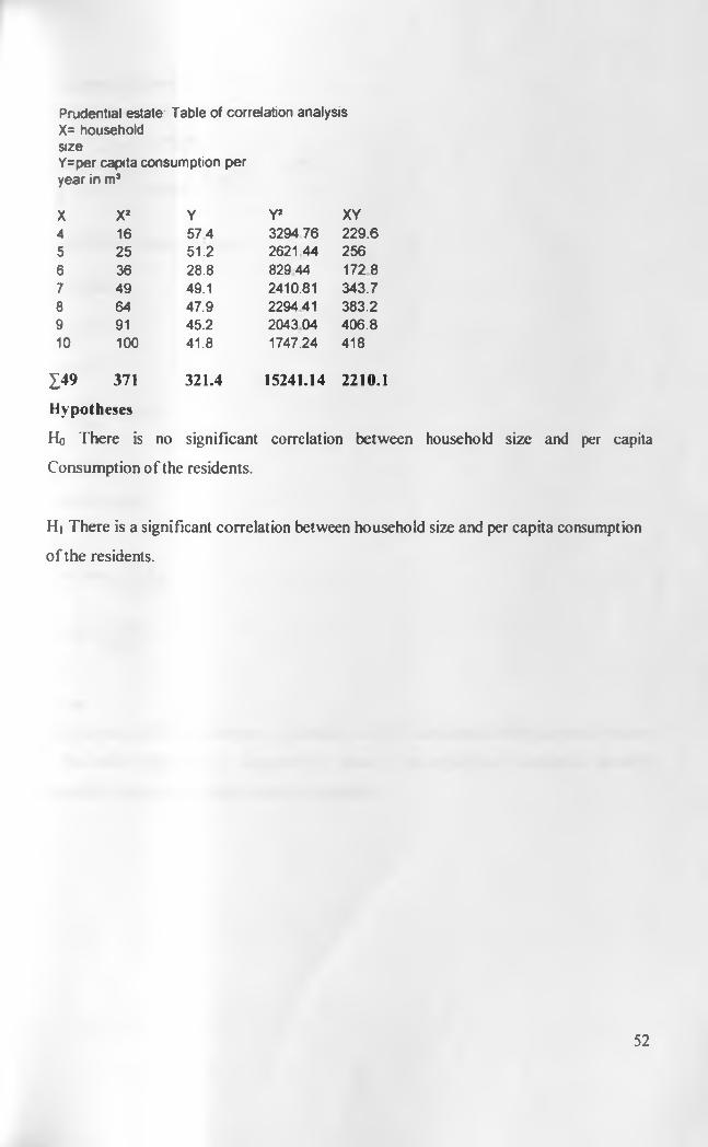
P rudentia l estate: Tab le o f co rre la tion ana lys isX= householdsizeY = per capita consum ption p e r year in m*

X X* Y Y* XY4 16 5 7 4 3294 76 2 29 .65 25 51.2 2621 44 2566 36 28.8 829 44 172 87 49 49.1 2410.81 343 .78 64 47.9 2294 41 383 .29 91 45.2 2043 04 4 06 .810 100 41.8 1747.24 418

149 371 321.4 15241.14 2210.1

Hypotheses

H0 There is no significant correlation between household size and per capita

Consumption o f the residents.

Hi There is a significant correlation between household size and per capita consumption

of the residents.

52

Prudential Estate

Correlation coefficient, (r) =

22.0 1

jL - My[ 7 J 7

= ^ (.3 7 1 -3 4 3 ) (15 2 4 1 .1 -1 4 7 5 6 .9 )

= V2&X484.2

= V13557.6

= 116.4

- 3 9 .7 116.4

= -0 .3 4 1 1

r 2 = 0.1163

r 2jr l0 0 = 11.63% HOr = 0H \ r * 0

I = .3 4 I I *1 -0 .1 1 6 3

/ = 0.86

Critical t at a 0.05 and 5 degrees o f freedom is 2.57. Calculated t, 0.86 is less than critical

t. The null hypothesis is adopted that there is no significant correlation between

household size and per capita water consumption.

53

4.2 b| UMOJA II SECTOR 1

Table 14. Household size and per capita consumption

Household Size Per capita consumption

2 25.9 m3

3 23.6 m3

4 25.3 m3

5 2 0 . 1 m3

6 19.6 m3

7 23.8 m3

g 28.9 m3

1 0 2 0 . 1 m3

Graph 2. Per capita consumption and household size

c0

1 »1 sI !3 •§Q. O (0 ok.So. 1 2 3 4 5 6 7 8 9 10

H ouseh old s iz e

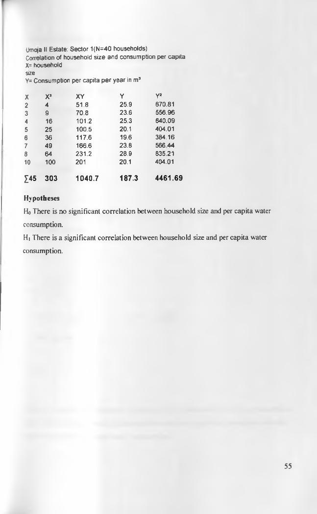
Umoja II Estate: S ecto r 1 (N = 40 househo lds)Correlation of household size and consumption per capitaX= householdsizeY= Consumption per capita per year in m*

X X* X Y Y Y*2 4 51.8 25.9 670.813 9 70.8 23.6 556.964 16 101.2 25.3 640 .095 25 100.5 20.1 404.016 36 117.6 19.6 384 .167 49 166.6 23.8 566 448 64 231 .2 28.9 835.2110 100 201 20.1 404.01

I A S 303 1040 .7 187 .3 4 4 6 1 .6 9

Hypotheses

Ho There is no significant correlation between household size and per capita water

consumption.

Hi There is a significant correlation between household size and per capita water

consumption.

55

, . , 0 4 0 , - < « & ! « >

V 5 J -! ,5 >1,4 4 6 .7 -M 8 8

Correlation coefficient, (r) =

= 1040.7 -1053.6 = -12.9

= 71 303-253.1 }t[4461.7-4385.2]

= 7149.9*76.5]

= 3̂817.35

= 61.8

-12.9r = —— = -0.2087 61.8

r2 = 0.0435

r* x 100 = 4.35% of consumption is accounted for by Household size.

Significance test or r

Ho r= 0

Hi r * 0

t = r- 2

1 - r 2

t = 0 .2087 XV6~

1 - 0.0435

= 0 2087 or 2 .5609

(0.2087i

2 4495

0.9565 J

1 = 0 .53

Critical t at a 0.05 and 6 degrees o f freedom is 2.45.Calculated t, 0.53 is less than critical

t, 2.45.The null hypothesis,Ho is adopted that there is no significant correlation between


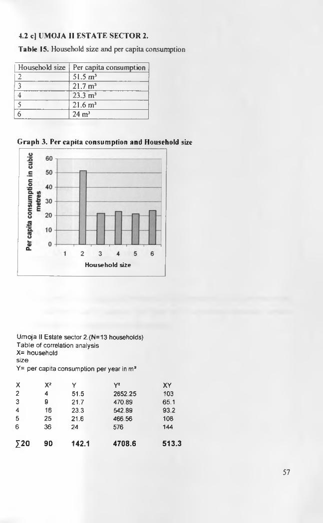
4.2 c) UMOJA II ESTATE SECTOR 2.

T able 15. Household size and per capita consumption

Household size Per capita consumption2 51.5 m3

3 21.7 m3

4 23.3 m3

5 2 1 . 6 m 3

6 24 m3

Graph 3. Per capita consumption and Household size

H ousehold size

U m o ja II Esta te sec to r 2 .(N = 1 3 households) T a b le o f co rre la tion a na lys is X — h ou se ho ld s izeY = p e r cap ita consum ption p e r year in m J

X X2 Y Y2 XY2 4 51.5 2652.25 1033 9 21.7 470.89 65.14 16 23.3 542 89 93.25 25 21.6 466.56 1086 36 24 576 144

£ 2 0 90 142.1 4708 .6 51 3 .3

57

Correlation coefficient r =

(20X142.1) _513.3- = 513.3-568.4 = -55.1

90 - 4708.6 (142 1Y

= V ( ^ '- 8 0 ) (4708.6 - 4038.5)

= V6701

= 81.9

-5 5 .181.9

= -0.6727

r 2 = 0 .4525 r 2*100 = 45.25

H O r = 0 t f l r * 0

I = 0.6727* V 5 - 21-0.4525

= 0 .6727* 1.73210.5475

/ = 2.13

Critical t at a 0.05 and 3 degrees of freedom is 3.18. Calculated t, 2.13 is less than critical

t. The null hypothesis is adopted that there is no significant correlation between


58

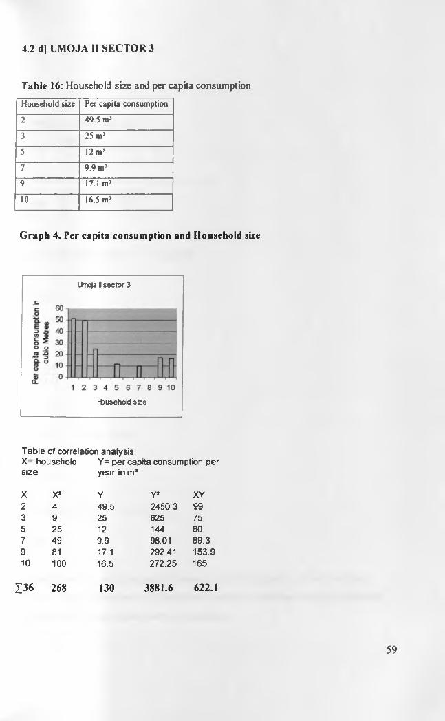
4.2 d| UMOJA II SECTOR 3

Table 16: Household size and per capita consumption

Household size Per capita consumption

2 49.5 mJ

3 25 m3

5 12 m3

7 9.9 m3

9 17.1 m3

10 16.5 m3

Graph 4. Per capita consumption and Household size

Umoja 0 s e c to r 3

Household size

T a b le o f co rre la tion ana lys isX — househo ld Y= p e r cap ita consum ption p e rs iz e ye a r in m s

X X 2 Y Y2 XY2 4 49.5 2450.3 993 9 25 625 755 25 12 144 607 49 9.9 98.01 69 .39 81 17.1 292.41 153.910 100 16.5 272.25 165

136 268 130 3881.6 622.1

59

Correlation coefficient (r) =

r =622 - £ 6-%— ^ = 6 2 2 -7 8 0 = -158

^268-216] l?882-2817j = V52jc1065

= V55380

= 253.33

-1 5 8253.33

r = -0 .6 2 3 7

r 2 = 0 .3 8 9 r 2*100 = 38.9%

H 0 r = 0 //| r *■ 0

/ = - 0 . 6 2 3 7 * — = 0 .6 2 3 7 *— - —1-0 .389 0.611

l = 2.04

Critical t at a 0.05, and 4 degrees of freedom is 2.78.Calculated t , 2.04 is less than

critical t. The null hypothesis is adopted that there is no significant correlation between


60

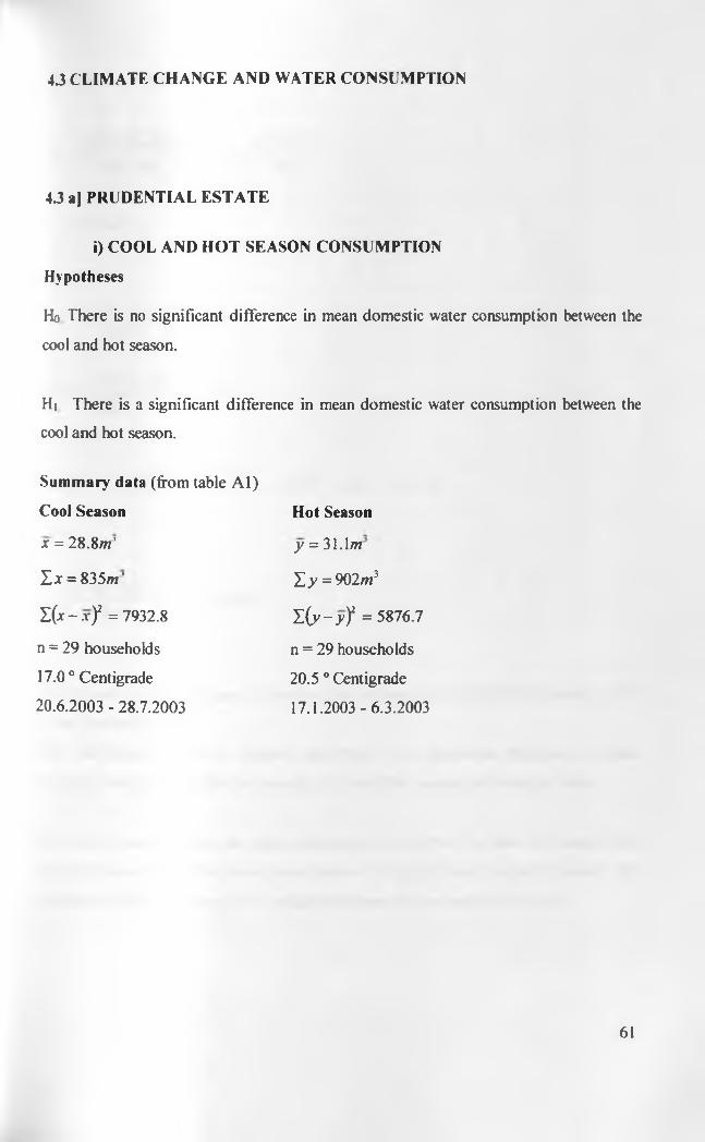
4J CLIMATE CHANGE AND WATER CONSUMPTION

4J a] PRUDENTIAL ESTATE

i) COOL AND HOT SEASON CONSUMPTION

Hypotheses

Ho There is no significant difference in mean domestic water consumption between the

cool and hot season.

Hi There is a significant difference in mean domestic water consumption between the

cool and hot season.

Summary data (from table A l)

Cool Season Hot Season

x = 28.8 m' y = 31.1/n

E y = 902m3

Z ( y - y f =5876.7

£ x = 835m'

I ( x - x f = 7932.8

n = 29 households

17.0 ° Centigrade

20.6.2003 - 28.7.2003

n = 29 households

20.5 0 Centigrade

17.1.2003 -6.3.2003

61

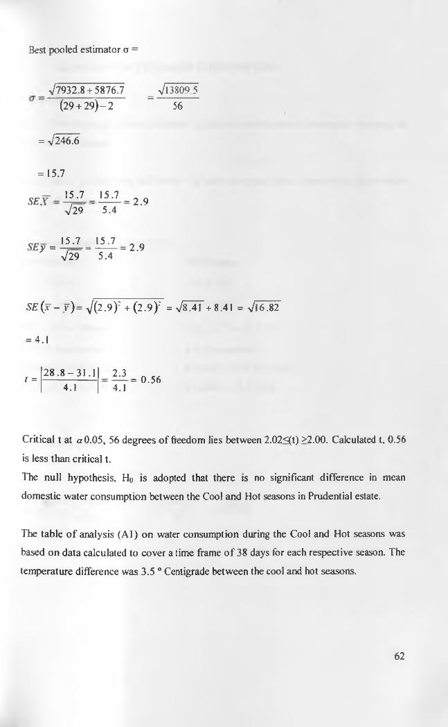
Best pooled estimator a =

77932.8 + 5876.7 _ 713809 5(29+ 2 9 )-2 “ 56

= 7246.6

= 15.7

SEX15.7 15.7729* ~~ 5.4

2.9

SEy = 15.7 _ 15.7 7 2 9*" 5.4

2.9

SE ( .7 - v)= yj{2.9): + (2 .9 ): =78.41 +8.41 = 7l6 .82

= 4.1

/ = 2 8 .8 -3 1 .14.1

2.34.1

= 0.56

Critical t at a 0.05, 56 degrees o f freedom lies between 2.02<(t) >2.00. Calculated t, 0.56

is less than critical t.

The null hypothesis, H0 is adopted that there is no significant difference in mean

domestic water consumption between the Cool and Hot seasons in Prudential estate.

The table o f analysis (A l) on water consumption during the Cool and Hot seasons was

based on data calculated to cover a time frame o f 38 days for each respective season. The

temperature difference was 3.5 0 Centigrade between the cool and hot seasons.

62

ii) DRY AND WET SEASON CONSUMPTION

Hypotheses


wet and dry season.


wet and dry season.

Summary Data (from table A2)

Dry Season

x = 36.2 in’

X* = 1050/w3

X(x - . ? ) 2 = 7844.8

n = 29 households

Rainfall: 26.4-43.3 mm

17.1.2003-6.3.2003

Wet Season

y = 32.1m3

X y = 930/n3

= 11191.9

n = 29 households


8.4.2003 - 22.5.2003


_ V7844.8+ 11191.9 Vl9036 7 /— 7 7 7 7

(29 + 29) - 2 " 56= 18.4

63

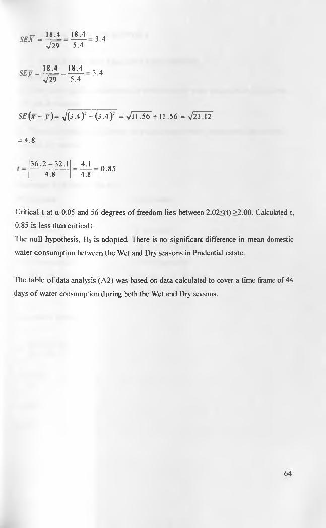
^ 18.4SEX => /2 9

18.45.4

3 .4

SEy =18.4 _ 18.4 V29 ” 5.4

3 .4

S £ ( x - v )= V(3-4 ) ' + (3 -4 ) ' = V ll.5 6 +11.56 = V23.12

= 4.8

3 6 .2 -3 2 .14 .8

4.14 .8

0.85

Critical t at a 0.05 and 56 degrees of freedom lies between 2.02<(t) >2.00. Calculated t,

0.85 is less than critical t.

The null hypothesis, Ho is adopted. There is no significant difference in mean domestic

water consumption between the Wet and Dry seasons in Prudential estate.

The table o f data analysis (A2) was based on data calculated to cover a time frame of 44

days o f water consumption during both the Wet and Dry seasons.

64

4.3 b] UMOJA II ESTATE SECTOR 1

i) WET AND DRY SEASON CONSUMPTION.

Hypotheses


wet and dry season.


wet and dry season.

Dry Season

y = 15.1m3

Y.y = 605m

l ( y - y f =4498.4

n= 40 households


3.1.2003 -19.2.2003

Best pooled estimator o =

>/810 + 4498.4 (4 0 + 4 0 ) - 2

_ V5308.4 78

= V68.06

= 8.25

Summary data (from table A3)

Wet Season

x = 8.5m3

Xx = 341m3

X ( x - x f = 8 1 0

n= 40 households


27.3.2003-14.5.2003

65

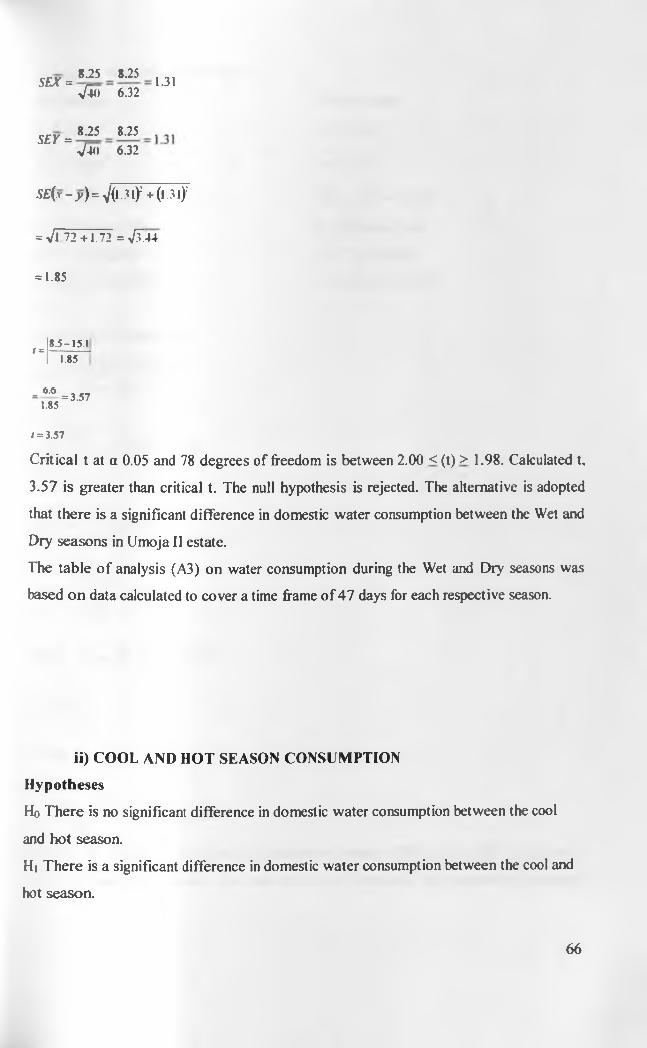
S E X =8.25 1L25• / io 6.32

1.31

S E Y =8.25 8.25 .V 40 6.32

S E (x-y )= J (D if + ( u i f

= V l 7 2+ 1 .7 2 = V ? 4 4

= 1.85

<= 8.5 -15 .1 1.85

= < * = 3 . 5 7 1.85

/ = 3.57

Critical t at a 0.05 and 78 degrees of freedom is between 2.00 < (t) > 1.98. Calculated t,

3.57 is greater than critical t. The null hypothesis is rejected. The alternative is adopted

that there is a significant difference in domestic water consumption between the Wet and

Dry seasons in Umoja II estate.

The table o f analysis (A3) on water consumption during the Wet and Dry seasons was

based on data calculated to cover a time frame o f 47 days for each respective season.

ii) COOL AND HOT SEASON CONSUMPTION

Hypotheses

Ho There is no significant difference in domestic water consumption between the cool

and hot season.

Hi There is a significant difference in domestic water consumption between the cool and

hot season.

66

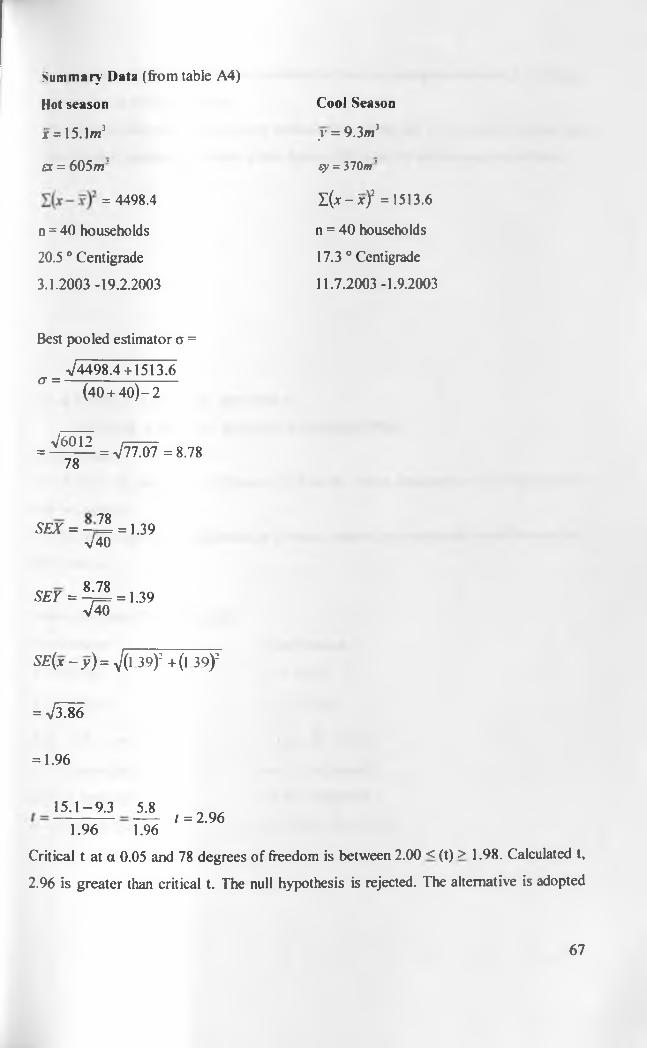
Cool Season

y = 9.3m3

ey = 370m ’

Z(jc - 3c) 2 = 1513.6

n = 40 households

17.3 ° Centigrade

11.7.2003-1.9.2003


= V4498.4 + 1513.6 ° (40+ 4 0 )-2

V6012 ,-------= - ------- = V77.07 = 8.78

78

Summary Data (from table A4)

Hot season

jr = 15.1m3

a = 605m'

= 4498.4

n = 40 households

20.5 0 Centigrade

3.1.2003-19.2.2003

SEX = - Z£ = 1.39 v40

SEY = - ^ 2 = 1.39 V40

SE(x - y ) = yl( 1 39): +(l 39):

= >/3^86

= 1.96

15.1-9 .31.96

5.81.96

I = 2.96

Critical t at a 0.05 and 78 degrees of freedom is between 2.00 < (t) > 1.98. Calculated t,

2.96 is greater than critical t. The null hypothesis is rejected. The alternative is adopted

67

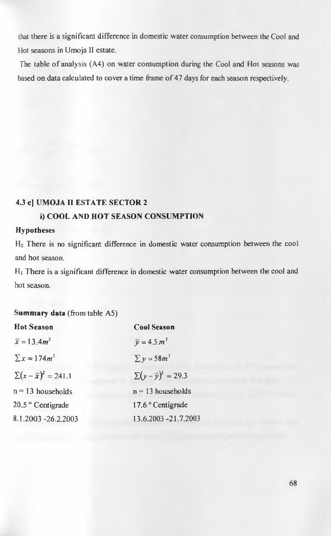
that there is a significant difference in domestic water consumption between the Cool and

Hot seasons in Umoja II estate.

The table o f analysis (A4) on water consumption during the Cool and Hot seasons was

based on data calculated to cover a time frame o f 47 days for each season respectively.

4.3 c) UMOJA II ESTATE SECTOR 2

i) COOL AND HOT SEASON CONSUMPTION

Hypotheses

H0 There is no significant difference in domestic water consumption between the cool

and hot season.

H| There is a significant difference in domestic water consumption between the cool and

hot season.


Hot Season Cool Season

Z(jc- x ) 2 = 241.1

x = 13.4m

Y.x = 174m3

y = 4.5.m3

Y.y = 58 m3

Z ( y - y ? =29.3

20.5 ° Centigrade

8.1.2003 -26.2.2003

n = 13 households n = 13 households

17.6 ° Centigrade

13.6.2003 -21.7.2003

68

^ p o o le d estimator a -

V270.424

= 3.36

_ 3.36 3.36

M 6 = 136 = 0 93 • Vl3 3.61

5£(x-JJ) = V(0.93): +(0.93):

=VTt J

= 1.32

13.4-4.5 _ 8.9 1.32 ~ T32

6.74

1 = 6.74

Critical t at a 0.05 and 24 degrees of freedom is 2.06. Calculated t. 6.74 is greater than

critical t. The null hypothesis is rejected. The alternative is adopted that there is a

significant difference in domestic water consumption between the Cool and Hot seasons

in Umoja II estate.The table o f analysis (A5) on water consumption during the Cool and Hot season,

on data calculated to c o v e r atime frame of 38 days for each season respectively.

69

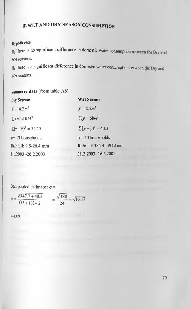
ii) WET AND DRY SEASON CONSUMPTION

Hypotheses

H„ There is no significant difference in domestic water consumption between the Dry and

Wet seasons.

Hi There is a significant difference in domestic water consumption between the Dry and

Wet seasons.

Summary data (from table A6 )

Dry Season

x = 16.2 m3

Ix = 210A/ 3

I(x -.r ) 2 = 347.7

n= 13 households


8.1.2003 -26.2.2003

Wet Season

v = 5.2 m3

"Ly = 6 8 w'

I ( y - > 7= 40 .3

n= 13 households

Rainfall: 384.4- 391.2 mm

31.3.2003-16.5.2003


(13 + 13)-2 24

= 4.02

70

v n 3 . 6 1

4.02 4.02 ,SEV = ~ r = = ------ = 1.11

Vl3 3.61

s E (x -y )= y l( \ i \ y + { \ n y

= y[2A6

= 1.57

16.2-5 .21.57

111.57

t = 7.01

Critical t at a 0.05 and 24 degrees o f freedom is 2.06. Calculated t, 7.01 is greater than


significant difference in domestic water consumption between the Wet and Dry seasons

in Umoja II estate.

The table o f analysis (A6 ) on water consumption during the Wet and Dry seasons was

based on data calculated to cover a time frame o f 46 days for each season respectively.

4.3 dj UMOJA II ESTATE SECTOR 3

i) HOT AND COOL SEASON CONSUMPTION

Hypotheses

Ho There is no significant difference in domestic water consumption between the Hot and

Cool seasons.

Hi There is a significant difference in domestic water consumption between the Hot and

Cool seasons.

71


Hot Season

x = 30.8m3

I * = 277m3

I ( x - . r ) 1 1 2 =3353.6

n = 9 households

20.5 ° Centigrade

8.1.2003 -28.2.2003

Cool Season

y = 7.7 m3

X = 69m 3

XCy-.v) 2 = 180

n = 9 households

17.3 ° Centigrade

17.7.2003 -4.9.2003


g _V 33S3.6 + 180 =(9 + 9 ) - 2 16

= 14.86

S E X = '- ± ™ = " ™ = 4.95 V9 3

pc_ 14.86 14.86SEy = — — = -------- = 4.95V9 3

SE(X - v )= ^(4 9 5 )' +(4 9 5 )'

= V24!? + 24.5 = >/49

= 7< _ 30.8-7 .7 | 23.1

7 7

1 = 3.3

Critical t at a 0.05 and 16 degrees of freedom is 2.12. Calculated t, 3.3 is greater than


significant difference in domestic water consumption between the Cool and Hot seasons

in Umoja II estate. The table o f analysis (A7) on water consumption during the Hot and

72

Cool seasons was based on data calculated to cover a time frame of 49 days for each

season respectively.

ii) WET AND DRY SEASON CONSUMPTION

Hypotheses

Ho There is no significant difference in domestic water consumption between the Dry and

Wet seasons.

Hi There is a significant difference in domestic water consumption between the Dry and

Wet seasons.


Dry Season

x = 32.1/w3

X x = 289m3

X ^ - .v ) 2 =3574.9

n = 9 households


8.1.2003 -28.2.2003

Best pooled estimator o =

ct= V35749+185.6

(9 + 9 ) - 2 16

Wet Season

y = 9.8m3

Y.y = 8 8 m’

l ( y - y ) 2 =185.6

n = 9 households

Rainfall: 384.4 -391.2 mm

31.3.2002-12.6.2003

= 15.91

73

SEX = 15.91 15.913

= 5.3

,V£v =15.91 _ 15.91 J 9 ~ 3

S £ ( f - y ) = | | t M

= V 56.18

= 7.5

t _ 32 .1 -9 .8 _ 22.3 7.5 ~ 7.5

t = 2.97

Critical t at a 0.05 and 16 degrees of freedom is 2.12. Calculated t, 2.97 is greater than


significant difference in domestic water consumption between the Wet and Dry seasons

in Umoja II estate.

The table o f analysis (A8 ) on water consumption during the Wet and Dry seasons was

based on data calculated to cover a time frame of 51 days for each season respectively.

74

4.4 IMPACT OF SOCIO-ECONOMIC STATUS ON CONSUMPTION

Hypotheses

Ho There is no significant difference in per capita water consumption between the

residents o f Prudential and Umoja II estates.

Hi There is a significant difference in per capita water consumption between the residents

of Prudential and Umoja 11 estates.


Prudential Estate

.V = 43.2 m3

£ * = 1253.4

£ ( * -3 F ) 2= 11801.24

n = 29 residents

Umoja II Estate

Y = 23 m3

£ k = 1426.1

£ ( v - r ) 2= 7090.85

n = 62 residents


(29+ 62)-214.57

S E X =14.57 14.57■J29 ~ 5.38 = 2.7

SEy =14,57

V62 = 1.85

S E (x -y )= V(T7)2 + (l -85)2 = -JloTi = 3.274 3 .2 - 2 3t =-----------

3.276.17

Critical t at a 0.05, 89 degrees o f freedom lies between 2.00<(t) >1.98.

Calculated t, 6.17, is greater than critical t.

Ho is rejected and the alternative is adopted that there is a significant difference in per

capita w ater consumption between residents of Prudential and Umoja II estates.

75

CHAPTER V

5.0 DISCUSSION OF RESULTS

Three important variables affecting water consumption were investigated. These

variables were Household size, Socio-economic status and Climate charge. The results

show that there is an order o f relative importance o f the variables. Household size had

least importance in terms of determining the water consumption per capita. The socio

economic status and climate change were important variables. The climatic changes

resulted in significant changes in per capita consumption in Umoja II estate. This means

that in order to plan properly and to effectively manage the water resource in cities,

seasonal and long-term climatic changes must be taken into account. The impact of socio

economic status on domestic water consumption was also found to be significant.

5.1.a) SEASONAL CHANGES AND DOMESTIC WATER CONSUMPTION

Table 17. Water consumption per household in Wet and Dry seasons

wet season consumption Dry season consumption Increment

Prudential estate 32.1 m3 36.2 m3 4.1 m3

Umoja II sector 1 8.5 m3 15.1 m3 6 . 6 m3

Umoja II sector 2 5.2 m3 16.2 m3 11 m3

Umoja II sector 3 9.8 m3 32.1 m3 22.3 m3

Table 18. Water consumption per household in Cool and Hot seasons

Cool season consumption Hot season consumption Increment

Prudential estate 28.8 m3 31.1 m3 2.3 m3


Um oja II sector 2 4.5 m3 13.4 m3 8.9 m3


A fter statistical analysis, it emerged that seasonal changes had an impact on the mean

w ater consumption of households in all the samples. However, it was noted that the

76

impact o f seasonal changes was not statistically significant in Prudential estate. The data

from table 19 shows that there was an increase in consumption o f 4.1 cubic metres

between the wet and dry seasons in Prudential. Although this was a clear increase due to

changes in climatic conditions, it was not statistically significant when subjected to the t-

test. Nevertheless, the fact was established that indeed a difference in mean household

consumption had occurred. The consumption in the dry season was higher than that o f the

wet season. The consumption in the cool season was also found to be lower than the

consumption during the hot season.

In general, the changes observed between the Wet and Dry season were higher than the

consumption changes between the Cool and Hot seasons. In prudential estate, the

percentage increase in consumption due to variation in rainfall was 1 2 .8 %, whereas the

changes in consumption due to temperature increase were 8 %. In Umoja II estate sector

1, the consumption increased by 77.6% from the wet to the dry season. The consumption

increased by 62.4% when the temperatures changed between the cool and hot seasons.

In Umoja II estate samples, it emerged that the changes in consumption that are attributed

to seasonal variations were statistically significant. At the end o f this discussion there is a

theory put forward to explain this differential impact of seasonal changes. This is the

phenomenon whereby seasonal changes had a greater impact in consumption in Umoja II

estate than in Prudential estate.

In all the 3 sectors sampled in Umoja II, the climatic changes were found to exert a

significant change in consumption of households. The differences in mean consumption

of the households were found to be statistically significant when subjected to the t-test.

The variations in climatic conditions caused changes in mean consumption of households

of such magnitude that these households behaved like entirely different populations based

on the prevailing climatic conditions. These changes were remarkable in that the sampled

households were in actual fact the same households, and that only the seasons had

changed. The seasonal changes in Umoja II resulted in the households acquiring entirely

different consumption characteristics. Since these differences were statistically

significant, the hypothesis stating that climatic changes have a significant impact on

domestic water consumption was adopted in Umoja II estate.

77

The alternative to this hypothesis had earlier been adopted in Prudential estate. In

Prudential estate the climatic changes had no significant impact on the mean consumption

of the sampled households. The differences in the way Umoja 11 households and the ones

in Prudential estate reacted to climatic changes suggests that domestic water consumers

will react differently to changes in climatic conditions based on their socio-economic

status. The reason why prudential estate consumption was only slightly altered by

seasonal changes, whereas the consumption in Umoja II was significantly altered is

explained in the theory put forward as follows.

5.1.b) IMPACT OF CLIMATIC CHANGES ON WATER CONSUMPTION

From the results, it was apparent that households of relatively higher socio-economic

status, represented here by Prudential estate, are likely to experience insignificant

changes in consumption due to variations in climatic conditions.

On the other hand, it became apparent that climatic variations have a significant impact

the domestic water consumption of households o f lower socio-economic status. The

following is an explanation for these observations.

The theory is that all species within the animal kingdom are sensitive to climatic

conditions, and that they respond to climatic changes primarily in one o f the following

two ways.

Response by;

a) Adaptation to climatic conditions, or

b) Modification of climatic conditions

What sets us apart from other animals is that as human beings, we are so greatly

concerned about the climatic conditions to the extent we monitor the climatic conditions

in the science o f Metreology.

78

a) Adaptation to climatic conditions

Adaptation: These are the changes in established behaviour patterns of animals in

response to changes in climatic conditions.

Animals may adapt to climatic changes by migration, for example. Other animals may

adapt physiologically by aestivation and hibernation. Moreover, these physiological

changes are accompanied by behavioural changes, as the affected animals usually adopt a

sedentary lifestyle during the adverse climatic conditions. Adaptation to climatic changes

thus involves changes in the behaviour of animals. Humans can also adapt to

environmental conditions by making behavioural changes. Any significant changes in

human behaviour in order to accommodate climatic changes invariably lead to changes

in domestic water consumption. Thus when human beings adapt to climatic changes, their

consumption patterns are inevitably altered.

b) Modification of climatic conditions.

Modification: This is the response to climatic changes by use of technologies that

alter adverse climatic conditions to suitable conditions.

Modification o f climatic conditions must involve the use o f technologies that alter

climatic conditions that are considered adverse into suitable climatic conditions.

Although the modification o f environmental conditions is chiefly the preserve o f human

beings, it is not limited to humans alone. A few animals are also able to modify their

immediate environments by use of simple technologies such as the weaving o f nests by

some birds.

Modification o f the environment is done by humans due to their sensitivity to changes in

climatic conditions. There is a vast array of technologies that can be used to modify

climatic conditions. For example, most humans live in constructed housing shelters. The

reason we live in constructed houses is principally to modify the climatic conditions to

suitable parameters. Homelessness among some people is a direct result of human

poverty, where the homeless cannot afford the high price o f building technology. In some

houses we have insulation, central heating and air conditioning systems to modify the

interior microclimatic conditions. The clothes we wear also modify the immediate

environment. Although whenever we dress up we may do it subconsciously, it is really a

79

modification o f climatic conditions. That is why we have winter and summer clothing for

example.

In order to modify the properties o f water, we have hot baths and instant hot showers for

example. Some technologies such as washing machines and dishwashers altogether

remove the need to make contact with water when washing clothes and dishes. The use of

technology to modify climatic conditions implies that human water consumption

potential remains unaffected by climatic conditions. However, all persons who cannot

afford such technologies have to adapt to adverse climatic conditions, and their water

consumption patterns are altered as a result.

It becomes apparent that in order to modify the immediate environment o f man, there is

always an economic cost involved. Usually this cost is incurred in purchasing the item

that modifies the environment. For example, in order to modify the temperature of cold

water in the house, one may opt to use an instant hot shower system. This will be costly

in terms o f initial purchase price and energy consumption. In the event a consumer uses

renewable energy such as solar energy, then only the initial purchase cost will be

incurred.

The consumer incurs an economic cost in order to modify the environment. The

involvement o f economic cost is the main criterion for the distinction between

modification and adaptation to environmental changes. Adaptation to environmental

conditions usually involves behaviour change, and does not necessarily involve

economic cost. In many cases adaptation to the climatic conditions is the cheaper option.

Since modification of the environment involves economic cost, it follows that having a

higher income makes a consumer better placed to modify his or her environment. Since

modification o f the environment does not necessitate significant behaviour changes, the

w ater consumption in households that can afford to modify their environments is not

significantly influenced by climatic changes.

On the other hand, the persons with low socio-economic status are more likely to react to

climatic changes by adaptation. Adaptation to the environmental conditions results in

behavioural changes. Adaptation is a lifestyle change.

80

Since Prudential estate residents represent a high-income population, they react to

changes in climatic conditions primarily by modification. That is the reason why the

consumption in Prudential estate was not significantly affected by the changes in climatic

conditions. Whenever the climatic conditions are modified, there is little need for

significant changes o f behaviour. The changes in behavior are in turn responsible for the

changes in consumption patterns, and so there is no expectation o f significant changes in

consumption in the absence o f behaviour change.

In Umoja II estate, the socio-economic status was relatively low compared to Prudential

estate. The changes in consumption in Umoja II were found to be statistically significant.

It is apparent that the Umoja II residents were more likely to adapt to changes in climatic

conditions than their Prudential estate counterparts. These changes in behaviour patterns

in turn resulted in a significant change in the water consumption patterns o f Umoja II

residents.

The socio-economic status determines the technological choices and behaviour of

consumers. The respondents were asked whether they boiled their tap water before

drinking to eliminate harmful microbes. The concerns on the safety of tap water arise

from the fact that the utility has been guilty o f providing untreated water to consumers on

several occasions in the past. As a result, 49% of respondents believed tap water was

unfit for direct consumption.

In prudential estate, 89 % of the respondents boiled their water to improve its quality. In

Um oja II estate, only 63% o f the respondents boiled their water. Although they had

concerns about the quality o f water, some of the Umoja II residents cited the cost

involved in boiling water as the reason for their failure to boil water.

81

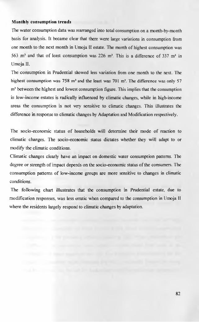
Monthly consumption trends

The water consumption data was rearranged into total consumption on a month-by-month

basis for analysis. It became clear that there were large variations in consumption from

one month to the next month in Umoja II estate. The month o f highest consumption was

563 m 3 and that o f least consumption was 226 m3. This is a difference o f 337 m3 in

Umoja II.

The consumption in Prudential showed less variation from one month to the next. The

highest consumption was 758 m3 and the least was 701 m3. The difference was only 57

m3 between the highest and lowest consumption figure. This implies that the consumption

in low-income estates is radically influenced by climatic changes, while in high-income

areas the consumption is not very sensitive to climatic changes. This illustrates the

difference in response to climatic changes by Adaptation and Modification respectively.

The socio-economic status o f households will determine their mode o f reaction to

climatic changes. The socio-economic status dictates whether they will adapt to or

modify the climatic conditions.

Climatic changes clearly have an impact on domestic water consumption patterns. The

degree or strength o f impact depends on the socio-economic status of the consumers. The

consumption patterns of low-income groups are more sensitive to changes in climatic

conditions.

The following chart illustrates that the consumption in Prudential estate, due to

modification responses, was less erratic when compared to the consumption in Umoja II

where the residents largely respond to climatic changes by adaptation.

82

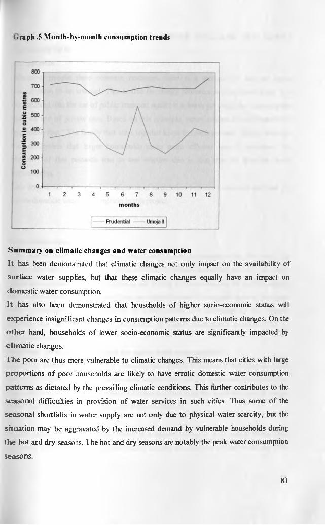
f.rapb .5 Month-by-month consumption trends

Summary on climatic changes and water consumption

I t has been demonstrated that climatic changes not only impact on the availability of

surface water supplies, but that these climatic changes equally have an impact on

domestic water consumption.

I t has also been demonstrated that households of higher socio-economic status will

experience insignificant changes in consumption patterns due to climatic changes. On the

o ther hand, households o f lower socio-economic status are significantly impacted by

clim atic changes.

T he poor are thus more vulnerable to climatic changes. This means that cities with large

proportions o f poor households are likely to have erratic domestic water consumption

patterns as dictated by the prevailing climatic conditions. This further contributes to the

seasonal difficulties in provision o f water services in such cities. Thus some o f the

seasonal shortfalls in water supply are not only due to physical water scarcity, but the

situation may be aggravated by the increased demand by vulnerable households during

the hot and dry seasons. The hot and dry seasons are notably the peak water consumption

seasons.

83

5.2 CORRELATION BETWEEN HOUSEHOLD SIZE AND PER CAPITA

CONSUMPTION

Introduction

Whenever people share common resources, there is a tendency o f the per capita

consumption to be lowered. This is true for energy resources such as fossil fuels. It is

documented that the use o f public transport results in a lower per capita fuel consumption

than the use of private cars. Based on this principle, many authors have advanced this

hypothesis that “ The family that stays together keeps the earth greener”. This is based on

the assumption that larger households make more efficient use o f resources. The

objective o f this research was to test whether this is also true for domestic water

consumption.

This hypothesis led to the investigation of correlation between household size and per

capita domestic water consumption in this project.

Correlation tests.

The significance of the correlation coefficient (r) was investigated using the t-test The

results showed that there was a weak correlation between household size and per capita

water consumption. In both Prudential and Umoja II estate samples, the null hypothesis

w'as adopted that there is no significant correlation between household size and per capita

water consumption. The coefficient o f determination, (r2) calculated for the samples

showed that the percentage or proportion o f water consumption accounted for by

household size was low

Summary on household size and per capita water consumption

In all the sampled households in Prudential and Umoja II estates, it emerged that there

was no significant correlation between household size and per capita water consumption.

The adoption o f the null hypothesis provides evidence that the water resource is unique

from other resources such as land and energy resources.

It was therefore concluded that water is a unique resource. It is unique from other

resources such as energy resources where sharing the resource at the household level

84

often leads to lower consumption per capita. For the water resource, individual needs are

not significantly lowered by virtue o f sharing the resource in a household setting.

The water consumption by one household member does not reduce the potential for

consumption by any other household members provided the level of water supply is

sustained.

85

5.3 IMPACT OF SOCIO-ECONOMIC STATUS ON DOMESTIC WATER

CONSUMPTION

Introduction

Disparities on domestic water consumption are based on socio-economic status. It was

hypothesized in this research that the households o f higher socio-economic status would

consume more water than their counterparts with a lower socio-economic status.

Prudential estate represented the higher socio-economic status and Umoja II represented

the lower socio-economic status population.

R esults

When the t- test was applied to the water consumption results, it was concluded that the

difference in per capita consumption between the two estates was statistically significant.

The null hypothesis was rejected and the alternative was adopted that there is a

significant difference in consumption between Prudential and Umoja II estates. This

significant difference in water consumption per capita was attributed to the difference in

socio-economic status between the two populations.

S u m m a ry

The socio-economic status determines the consumption patterns of consumers as well as

the technological choices that they make in their houses. Some technologies may result in

water use efficiency while others may not. In Prudential estate, 59% of the respondents

made use o f showers for personal hygiene, while 41% used basins to bathe themselves. In

Umoja II estate, the choice o f technologies was different. Only 23.5% of the respondents

made use o f showers .The majority o f respondents, 76.5% used basins to wash their

bodies. In Umoja II, one o f the reasons given for low usage of showers was that some o f

their bathrooms were not fitted with shower facilities.

Another reason given for widespread use of basins in Umoja II was lack o f sufficient

water pressure in the showers. This low pressure may be due to inefficiency on the part of

the water utility company, coupled with a high demand from a large population that

exceeds the infrastructure capacity.

86

Factors co n trib u tin g to pe r c a p ita w ater consum ption

a) Total living space

b) Income levels

c) Water pricing policy

• Houses with larger total living spaces require larger amounts o f water to maintain the

houses. Small-sized houses require less water for general house maintenance. A house

with many rooms and a sizeable garden or lawn requires more water. In this research.

Prudential estate houses have 4 bedrooms and a servant’s quarter. The gardens in

Prudential were also well watered. The expansive living space contributed to the high

water consumption in Prudential estate.

• Income levels contribute to the per capita water consumption of individuals. High

income creates additional demands for water, and determines the means by which

water is made available to consumers. For example, the economically poor

populations that live in Nairobi’s informal settlements do not have piped water

supplies. They mostly obtain their water from vendors. On the other hand, the wealthy

have a ready supply of piped water that is directly accessible within their houses. In

addition, the large total living space, and various household goods acquired as a result

o f wealth create greater demand for water. • •

• Pricing policies also determine the water consumption patterns of consumers. For

instance, the water for Prudential and Umoja II estates was priced at the same rate by

the utility. This gives little or no incentive to the high-income households to use water

resources conservatively. The pricing of water has political and economic

implications. As a result, the water resource is often under-priced for political reasons.

When water is not priced on sound economic basis, there is little motivation for the

consumers to conserve water. Thus poor pricing policies contribute to high water

consumption

The three factors discussed above all contributed to the higher water consumption in

Prudential estate than in Umoja II estate.

87

Coping w ith w a te r shortages

The residents of Nairobi cope with water shortage by stockpiling water. Some of the

houses have inbuilt tanks that act as water reservoirs. Some of the residents buy

additional large capacity tanks and water containers to store water. The following is a

picture o f a water storage tank in Umoja II estate.

Photo IX . W ate r storage ta n k in a house com pound Umoja II

The stockpile of water in each house ensures there is little disruption to normal water

consumption in periods o f water shortage. Water shortages are usually experienced

whenever there are repairs and maintenance o f works, and also during severely dry

seasons. The ability to stockpile water in households renders any water rationing

activities by the utility futile (Budds and Me Granahan, 2003). The consumers over

abstract water when it is available, and later use these reserves during the period of water

shortage. These are the mechanisms by which the city residents cope with water

shortages.

W a te r co nserva tion ethics.

There was no clear evidence o f water conservation ethics in any o f the sampled

households in Prudential and Umoja II estates.

In Prudential estate, 49 % o f the respondents felt water was expensively priced. They

however did not make any notable efforts to conserve water.

88

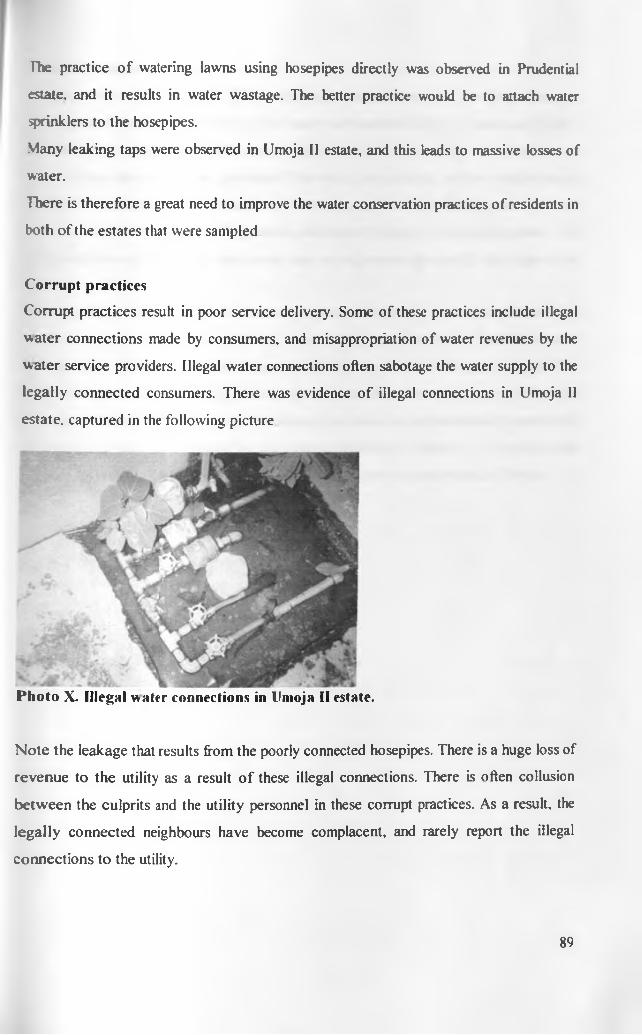
The practice o f watering lawns using hosepipes directly was observed in Prudential

estate, and it results in water wastage. The better practice would be to attach water

sprinklers to the hosepipes.

Many leaking taps were observed in Umoja II estate, and this leads to massive losses of

water.

There is therefore a great need to improve the water conservation practices o f residents in

both o f the estates that were sampled

C o rru p t p rac tice s

Corrupt practices result in poor service delivery. Some of these practices include illegal

water connections made by consumers, and misappropriation of water revenues by the

water service providers. Illegal water connections often sabotage the water supply to the

legally connected consumers. There was evidence o f illegal connections in Umoja II

estate, captured in the following picture

Photo X. Illegal water connections in llmoja II estate.

N ote the leakage that results from the poorly connected hosepipes. There is a huge loss of

revenue to the utility as a result o f these illegal connections. There is often collusion

between the culprits and the utility personnel in these corrupt practices. As a result, the

legally connected neighbours have become complacent, and rarely report the illegal

connections to the utility.

89

VS ater management in Kenya

In Kenya the body responsible for management of water is known as the Water Resource

Management Authority (WRMA). This body was constituted by the water act (2002).

The WRMA is charged with the responsibility, inter alia, of ensuring that all catchment

areas within the country are protected. This is to be achieved by the constitution of

catchment protection committees in all water catchment areas. Catchment protection

activities include the control o f vegetation, soil conservation and forest preservation. The

main objective o f protecting catchment areas is to preserve the quality and quantity of

water.

Other civil society groups and relevant government agencies are also involved in

catchment protection. An example o f a successful group is the Green Belt Movement.

This group is led by the 2004 Nobel peace prize laureate, Professor Wangari Maathai.The

G reen Belt Movement is involved in tree planting exercises across the country. They also

play the role o f a watchdog body that sounds the alarm on environmentally destructive

practices that may be condoned by the political leadership in Kenya. The group also

focuses on ways to ensure local communities are involved in conservation of forests.

90

Areas for further research

• This research did not investigate the particular behaviour changes that result in lower

consumption in cool seasons when compared to the hot season. ITiese behaviour

changes are subtle and may not be easily noticed. However, it has been established

that these subtle behaviour changes can become statistically significant between one

season and the next.

• Another area for further research is to look into the possibility of quantifying and

determining the strength o f correlation between climatic changes and consumption

changes. It was not possible to determine the precise increase in consumption brought

about by a single degree’s increase in temperature. It would be desirable if the data

could allow for the calculation of how much change in consumption can be attributed

to a degree increase in temperature and to an increase in rainfall. Such information

could be useful in the preparation o f future water consumption models. One of the

conditions for achieving this is through making data on climatic conditions available

on a day-to-day basis. Such data was not accessible from the Metreology department

during the course of this research. For example, the data they presented had a total

number o f rainy days in a month, but the particular dates of the rainy days were not

provided in their compiled data. It was not possible to gain access to the raw data

during the course o f this research. Such raw data needs to be made easily accessible to

researchers in future. • •

• It was apparent from the results that temperature changes played a lesser role in

determining water consumption when compared to rainfall changes. It may thus be

concluded that rainfall is a slightly more important factor of climate change in

determining water consumption than temperature changes. However, this is an area

that requires further research, as often rainfall and temperature act synergistically, and

it is difficult to describe the impact of the two factors separately.

91

• The aspect o f gender o f the respondents was not investigated due to the primary

assumption o f the per capita water consumption. It was assumed that there is no

difference in consumption based on age, size and gender. However, further research is

needed to determine the role o f gender in water consumption. The results o f such

investigations could lead to the development a gender- based water consumption

indicator.

92

5.4 a) Practical and academic significance of the study

Contribution to the discipline

o The methodology used to determine the impact of climatic conditions on domestic

water consumption was new to the field. The research clarified the importance of

climate change in domestic water consumption,

o The research affirms previous results that report a difference in water consumption

based on socio-economic status of consumers. It was affirmed that per capita water

consumption is high in high-income estates, and the per capita water consumption is

lower in low-income estates.

o In the course of the work, it was clarified that response to climatic changes are based

on socio-economic status o f a population. It is clarified that consumer response to

climatic changes is by either Adaptation or by Modification. It was further clarified

that modification o f climatic conditions is the likely response for affluent populations.

Less affluent populations respond to climatic changes primarily by adaptation,

o In the course of the research, new data was produced regarding water consumption in

Nairobi. This new data fills some of the knowledge gaps left by previous researchers.

5.4 b) Practical and academic recommendations o f the study.

R o le o f th e G overnm en t

■ Government development policy should focus on sustainable development. The

government should fully participate in initiatives to manage human induced climate

change. The Kenyan commitment to the Kyoto protocol should be sustained. Clear

policies should be formulated and fully implemented to curb production of Green

house gases. This is because climate change could have a severe impact on both water

consumption patterns and on water availability. The implications of climate change on

natural systems sustaining humanity may be more serious than previously thought

(Ong'wenyi, 2000)

■ The policy makers should involve local participation from city residents, and adopt the

bottom-up management approach. This is because water management is more than a

93

scientific and engineering issue, but one that extends to include community

empowerment and organizational restructuring (Syed & Nickum, 2002).

• The forest cover of the country should be increased, and water catchments conserved.

The government should pay due attention to these sectors in its development plans.

Role of consumers

■ Consumers should be encouraged to conserve water in their households. This

conservation can be achieved by reusing water and prompt replacement o f leaking

taps.

■ Consumers should be encouraged to report corrupt water practices such as illegal

connections to the authorities.

Domestic water conservation measures

The following measures can help consumers in reducing the amount o f water required for

general household activities.

> Retrofitting o f houses is the process of replacing old systems with modem water

efficient devices that lead to lower water consumption. Low capacity cisterns are

available and should be used to replace wasteful high capacity cisterns.

> Consumers are encouraged to reuse water in the houses. Brown water is water that has

been use for laundry, and may be reused to flush cisterns instead of being poured

down the drain.

Consumers who wash their cars using water poured directly from hosepipes ought to

use basins instead so as to conserve water. Consumers with gardens and lawns have

the option o f using efficient sprinklers to water their lawns instead o f direct hosepipes.

Another option is for residents to grow drought resistant plants in their gardens. There

are various species o f plants that have a high ornamental value and low water

requirements.

> The use o f showers instead o f basins and bathtubs for personal hygiene lowers the

w ater consumption per capita. Consumers should be encouraged to use shower

facilities.

94

Role of water service providers

■ The water service providers should reduce leakages in their water storage and

distribution network. It has been estimated that a 20% - 25 % reduction o f current

water losses (unaccounted for water) could eliminate water shortage problems in

Nairobi (UNESCO/UN, 2003).

■ The water service providers should be actively involved in the protection o f catchment

areas.

■ The pricing policies should be reviewed constantly by the utility in consultation with

lead government agencies and all stakeholders.

■ There is need to invest in technologies relating to water reuse and recycling o f water.

Research should be intensified in non-conventional sources of water such as

desalinization.

5.4 c) Conclusion

Domestic water needs of a growing city population in Nairobi can be met in a sustainable

manner if these recommended measures are implemented, and if the water resource is

given a priority in government planning. Proper water management often results in better

quality o f life, and leads to the achievement of the ultimate goals of sustainable socio

economic growth.

95

BIBLIOGRAPHY

Alcamo, J. et al, “Global Change and Global scenarios of Water Use and

Availability: An Application of Water GAP 10 model” in Gash et al, (eds.) (2001)

Biospheric Aspects of the Hydrological Cycle. BAHC international project office,

Potsdam, Germany.pg.l 12-3.

Animashaun, I.A, “Environmental problems in African cities” in African Urban

Quarterly. Special issue on Urban and Regional Planning of Nigeria. Vo 1.4 no. 1&2,

January and May 1989.pg 43-58

Arntzen, Jaap., “Sustainable Water Management in Southern Africa: An Integrated

Perspective” in Gash et al, (eds,) (2001) Biospheric Aspects of the Hydrological

Cycle. BAHC international project office, Potsdam, Germany pg.82-86.

Boreham,A.J and Semple,M. “Future development of work in the government

statistical service on the distribution and redistribution of household income” in

Atkinson, A.B (ed) (1976) The Personal Distribution of Incomes. George Allen and

Unwin Limited, London. Pg. 274-276.

Budds, Jessica and McGranahan, Gordon “Are the debates on water and

privatization missing the point? Experiences from Africa, Asia and Latin America" in

Environment and Urbanization Vol.15 No.2, October 2003. Pg.87-113.

Chalecki, L. Elizabeth & Wong, Arlene, “Measuring Water Well-being: Water

Indicators and Indices” in Gleick et al (eds,). (2002) The World's Water: The

Biennial Report on Freshwater Resources. 2002-2003.Pacific Institute for Studies in

Development, Environment and Security &Island Press, Washington, Covelo,

London, pg .87-93,106,250,303-7.

Cosgrove, W.J., and Rijsberman, F.R. (2000) World Water Vision: Making Water

Everybody’s Business World Water Council, Earthscan publishers, London pg.49

De Bruin,H.A.R., “Evaporation in Humid Tropical Regions” in Keller,R.(ed) (1983)

Hydrology of Humid Tropical Regions. International Association of the Hydrological

Sciences (IAHS) publicationno.140, Pg.299-308.

De Vries et al “Environmental reporting” in Bakkes, J.A and J.W. van Woerden (eds)

(1997) The Future of the Global Environment: A Model-based Analysis Supporting

UNEP’S First Global Environment Outlook. UNEP, Nairobi, Kenya. Pg.91, 113,149.

96

Durand, Roger and Alison, C.Richard. “Water Management in Urban Areas” in

Loethen, Mark. L. (ed)(1995) Proceedings o f AW RA’s 31*. Annual Conference and

Symposia. American Water Resources Association. Herndon Press, Virginia Pg.337-

348

Frost, Peter G.H, “Reflections on Integrated Land and Water Management” in Gash

et al (eds) (2001) Biospheric Aspects o f the Hydrological Cycle) BAHC International

Project Office, Potsdam, Germany pg.54-5

Gash, John. H.C., Odada, E.O., Oyebande. Lekan, & Schulze, R.E. (eds) (2001)

Biospheric Aspects of the Hydrological Cycle) BAHC International Project Office,

Potsdam, Germany.Pg.9-14, 29,54,82-85,98,113.

Gash, John. H.C., Wallace.J, Bonell, M. & Shuttleworth.W. “Hydrology for the

Environment, Life and Policy (HELP): A New Worldwide Hydrology Initiative” In

Gash et al (eds)(2001) Biospheric Aspects o f the Hydrological Cycle) BAHC

International Project Office, Potsdam, Germany .Pg 112-5

Gleick, Peter. (1992) Water Conflict. Occasional Paper Series o f the Project on

Environmental Change and Acute Conflict. A Joint Project o f University o f Toronto

and the American Academy o f Arts and Science.No. 1, Sept, 1992

Gleick, Peter et al. (eds) (2002) The World’s Water: The Biennial Report on

Freshwater Resources. 2002-2003.Pacific Institute for Studies in Development,

Environment and Security &Island Press, Washington, Covelo, London. Pg.

99,103,250.

Gleick, Peter H. (ed)(1993) Water in Crisis: A guide to the World's Freshwater

Resources. Oxford University Press, Oxford & New York. Pg. 3-13,80-92, 105-

9,124-9,171 -9,187-190,223,374,411-413.

Government of Kenya- Ministry Of Planning and National Development (1998)

First Report on Poverty in Kenya. Volume 2:Povertv and Social Indicators. Pg 85-90.

Government of Kenya(1974) National Development Plan 1974-1978 Government

Printer, Nairobi.Pg.324-342.

Government of Kenya(1997) National Development Plan 1997-2001.Government

Printer, Nairobi.Pg.324-42.

97

Harrison, Paul (1992) The Third Revolution: Population. Environment and a

Sustainable World. Penguin Books. New York. Pg 239-40,306-7.

Iteke, H.K.E. “Water Conservation-the Cellular Approach” in West African

Technical Review. November 1980. Pg. 41-4.

Jaeger, Carlo, C. “Water Resources and Social Conflict” in Gash et al (eds)(2001)

Biospheric Aspects o f the Hydrological Cycle) BAHC International Project Office,

Potsdam, Germany Pg.21-39.

Jones, J.A.,(1997) Global Hydrology: Process, Resources and Environmental

M anagem ent-Long m an.Pg.49

Khroda,G.O. “Hydrology, Water Supply and Source Regions o f Migration in Kenya:

Towards a planning Strategy” in African Urban Quarterly Vol.3 no.3&4, August-

November 1988. Pg.265-76.

Khroda,G.O “Water Supply in Kenya-Today and the Year 2000 .A.D.” in Ominde,

S.H(ed) 1988) Kenya’s Population Growth and development to the Year 2000 A.D.

Heinman, Nairobi.

Lamba, Davinder “The Forgotten Half: Environmental Health in Nairobi’s Poverty

Areas.” in Environment and Urbanization Vol.6, N o.l, April 1994. Pg. 164-73.

Lekan Oyebande “Urban Climatology in Africa” in African Urban Quarterly Vol.5,

No.l&2, Feb and May 1990.Pg .39-48,59-65.

Lillis, Kevin.M “Urbanization and Education in Nairobi, Kenya” in African Urban

Quarterly Vo 1.7 No. 1 &2 1991. Pg.99-102.

Makuro, Mike “Coping with the Drought in Nairobi” in Water for African Cities

Issue3, July-September 2000.(Unchs-Habitat) and UNEP.Pg.3-4

Odhiambo, Thomas, R. “Training o f a New Generation o f African Freshwater

Managers” in (2001) Biospheric Aspects o f the Hydrological Cycle. BAHC

International Project Office, Potsdam, Germany, Pg 15.

Ogembo, W ,0. “Assessment o f water resources in Kenya-with some aspects of their

rational utilization” UNESCO/IAHR seminar on hydraulic research and river basin

development. September 1980,Nairobi.Pg.6,7.

Ong’wenyi , G.S et al. “The impact o f climate change on land and water resource

management in Kenya” in (2000) Gichuki ,F.N. et al (eds) Land and water

98

management in Kenya: Towards sustainable land use. English Press ,Ltd. Nairobi.

Pg.219

Oucho, John.O. “Freshwater and Population Dynamics in Africa” in Gash et al

(eds)(2001)Biospheric Aspects o f the Hydrological Cycle) BAHC International

Project Office, Potsdam, Germany. Pg.33-41.

Peil, Margaret “Situational Variables” in Bulmer, M. and Warwick. D.P (eds)(1983)

Social Research in Developing Countries. John Wiley and Sons, New York. Pg.71-

88.

P e tre lla , R iccardo (2001). The Water Manifesto. ZED Books, London, U.K. Pg.24-

32,40-1, 14-5.

Porter, Richard.C et al (1997) The Economics o f Water and Waste in 3 African

Capitals. Ashgate Publishing, England & U.S.A.Pg.2-7,43-7, 73.

Postel, Sandra “Facing Water Scarcity” in Lester, R. Brown(ed) State of The World

19930 993) Worldwatch institute, W.W. Norton & Co. New York.

Rosegrant, M ark., Ximing, Cai., & Sarah, A.CIine. (2002)World Water and Food

to 2025:Dealing with Scarcity. International Food Policy Research Institute,

Washington, D.C. Pg.140.

Rotmans, J. et al “Environment System Models” in UNEP/RIVM (1995) Swart R,

J. and Bakkes J, A. (eds) Scanning the Global Environment: A Framework and

Methodology for Integrated Environmental Reporting and Assessment.

UNEP/EATR.95-01, RIVM 402001002. Environmental Assessment Sub-programme,

UNEP, Nairobi. Pg.30.

Saghir, J., Schifler, M., and Woldu, M. (1997) World Bank Urban Water and

Sanitation in the Middle East and North Africa Region: The Wav Forward. The

World Bank & North Region Infrastructure Development Group.

www.worldbank.org/wbi/mdf7mdD/papers/finance/Saghir.pdf

Schulze, Roland.E. “Managing Water as a Resource in Africa: Are We Asking the

Right Questions in the Quest for Solutions?” in Gash et al(eds)(2001) Biospheric

Aspects o f the Hydrological Cycle) BAHC International Project Office, Potsdam.

Germany Pg.9-14.

99

http://www.worldbank.org/wbi/mdf7mdD/papers/finance/Saghir.pdf

SEI/ UNEP (1998).Bending the Curve: Toward Global Sustainability. Pole Star

Series Report No.8, 1998; UNEP/DEIA TR-98-4, Nairobi, Kenya. Pg. 23-5,55-61.

Shaw, Paul. “The Impact of Population Growth on Environment: The Debate Heats

Up” in Environmental Impact Assessment Review Vol.120, March 1992.Elsevier.

Pg-11-36.

Shildomanov, LA. “World Water Resources” in Gleick, P.H.(ed) (19931 Water in

Crisis. Oxford University Press, Oxford, New York. Pg. 13-24.

So et al, “Water: Facts of Life” in American Water Works Association Journal

Vol.74, No.6 1982.Pg 11.

Sved, Ayub.Q, and Nickum, James.E. “Civil Society and Water Management in the

Indus Basin” in Regional Development Dialogue Vol.23, No.l, Spring 2002. Pg.109-

117.

Tebbutt, T.H.Y (1990). Basic Water and Wastewater Treatment Butterworth &

Company, London.Pg.10-17.

Thompson, John et al “Waiting At the Tap: Changes in Urban Water Use in East

Africa Over Three Decades” in Environment and Urbanization. Sustainable Cities

Revisited 3. Vol.12 No.2, October 2000. Pg 37-52.

UNEP/HABITAT (1999) Sustainable Cities Programme. (SCP1 Sourcebook Series

institutionalizing the (EPM1 Environmental Planning and Management Process.

UNEP/HABITAT, Nairobi. Pg.67-70.

UNEP/DEIA. (1996). Rump, P.State of the Environment Reporting: Source Book of

Methods and Approaches. UNEP/DEIA/TR.96-1. UNEP, Nairobi, Kenya._ Pg.42,

54-6,85-6.

UNEP-IETC (1999).International Environmental Technology Centre. International

Symposium on Efficient Water Use in Urban Areas-Innovative Ways o f Finding

Water fo r Cities. 8-10th. June 1999. UNEP-IETC, Kobe, Japan. Pg.3,4 ,289,301-3.

UNEP(2002) L'avenir de L'environnement en Afriaue: Le passe, Le Present et les

Perspectives de L’avenir.Nairobi.Pg. 157-62, 167-70.

UNESCO (20031 Water for People. Water for Life: The UN World Water

Development Report UNESCO& Berghahn books. Pg. 12.48.68-9,76,90,95, 157-162.

100

UN-HABITAT. Water and Sanitation in the World’s Cities: Local Action for Global

Goals (2003). United Nations Human Settlements Programme (UN-

HAB1TAT)/Earthscan Publications, London. Pg.6,27-30, 57,66,78,129-138.

UNICEF/ Government of Kenya. (1990) Socio-economic Profiles: Nairobi City.

(June 1990) UNICEF/ Ministry o f Planning and National Development, Government

o f Kenya. Pg. 175-80.

Electronic sources

www.mapquest.com

www.hassconsult.co.ke

www.worldwaterforum.org

www. waterwiser. org/wtruse98/main. ht ml

CIA world fact book-Kenya: www.odci.gov/cia/publications/factbook/geos/ke.html

101

http://www.mapquest.com

http://www.hassconsult.co.ke

http://www.worldwaterforum.org

http://www.odci.gov/cia/publications/factbook/geos/ke.html

APPENDIX A

DATA ANALYSIS TABLES

P ru d e n tia l E s ta te (N=29 househo lds)C o n s u m p tio n in th e Cool and Hot seasonC o o l S eason Hot Season

Table A1

(X -X ) (X -X ) ’ Y (Y-Y) (Y -Y )*12 -16.8 2 8 2 .2 4 32 0.9 0.8131 2.2 4 .8 4 17 -14.1 198.8143 14.2 201 .6 4 36 4 .9 24.0126 -2.8 7 .84 26 -5.1 2 6 0 1

8 -20 .8 4 3 2 .6 4 13 -18.1 327.6122 -6.8 4 6 .2 4 21 -10.1 102.0136 7.2 51 .84 35 3.9 15.2165 36.2 1310.44 63 31.9 1017.6120 -8.8 77 .44 23 -8.1 65.6131 2.2 4 .84 36 4 .9 24.0143 14.2 2 0 1 .6 4 46 14.9 222.0143 14.2 201 .6 4 29 -2.1 4 4 125 -3.8 14.44 48 16.9 285 6 152 23.2 538 .24 62 30.9 954 8157 28.2 795 .24 49 17.9 320.4142 13.2 174 .24 40 8.9 79.2122 -6.8 4 6 .2 4 27 -4.1 16.8113 -15 .8 249 .6 4 18 -13.1 171.61

9 -19 .8 392 .0 4 35 3.9 15.2162 33.2 1102.24 47 15.9 252.8117 -11.8 139 .24 27 -4.1 16.8121 -7.8 6 0 .8 4 32 0.9 0 8 1

5 -23.8 566 .44 2 -29.1 846 8114 -14.8 219 .0 4 13 -18.1 327.6128 -0 .8 0 .6 4 31 -0.1 0.0110 -18.8 353 .44 21 -10.1 102.0134 5.2 2 7 .04 34 2 .9 8.41

9 -19.8 392 .04 10 -21.1 445 2135 6.2 38 .44 29 -2.1 4 4 1

£835 7932.76 902 5876.69

102

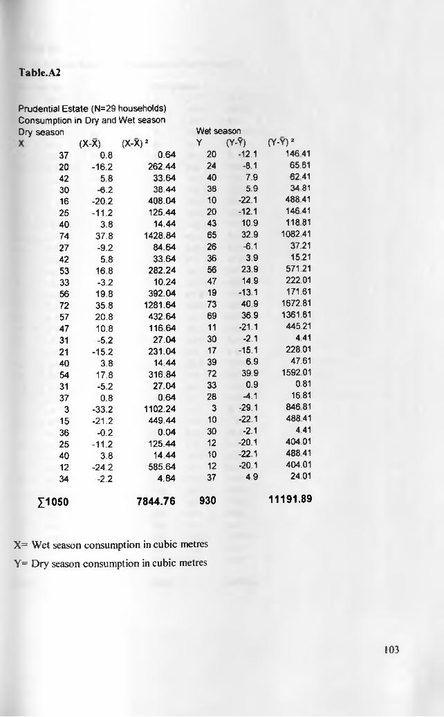
Table.A2

P rud e n tia l E s ta te (N =29 househo lds)C o n sum p tion in D ry and W e t seasonD ry season W et season

(X -X ) (X -X ) ’ Y (Y-?) (Y -Y ) ’37 0.8 0 .64 20 -12.1 146 4120 -16 .2 262 .44 24 -8.1 65.6142 5.8 33 .64 40 7.9 6 24130 -6 .2 38 .44 38 5.9 34 8116 -20 .2 408 .0 4 10 -22.1 4884125 -11 .2 125 .44 20 -12.1 146 4140 3.8 14.44 43 10.9 1188174 37.8 1428.84 65 32.9 10824127 -9 .2 84 .64 26 -6.1 37.2142 5.8 33 .64 36 3.9 15.2153 16.8 282 .24 56 23.9 571.2133 -3 .2 10.24 47 14.9 222.0156 19.8 392 .04 19 -13.1 171.6172 35.8 1281.64 73 40.9 1672.8157 20.8 432 .64 69 36.9 1361.6147 10.8 116.64 11 -21.1 445.2131 -5 .2 27 .04 30 -2.1 44121 -15 .2 231 .04 17 -15.1 228.0140 3.8 14.44 39 6.9 47.6154 17.8 316 .84 72 39.9 1592 0131 -5 .2 2 7 .04 33 0.9 0.8137 0.8 0 .64 28 -4.1 16.81

3 -33 .2 1102.24 3 -29.1 846 8115 -21 .2 449 .44 10 -22.1 4884136 -0 .2 0 .04 30 -2.1 4.4125 -11 .2 125.44 12 -20.1 404 0140 3.8 14.44 10 -22.1 4884112 -24 .2 585 .64 12 -20.1 404 0134 -2 .2 4 .84 37 4.9 2 401

£1050 7844.76 930 11191.89

X= Wet season consumption in cubic metres

Y= Dry season consumption in cubic metres

103

Table A3U m o ja II E sta te S e c to r 1 C onsum ption o f the W et and Dry s e a s o n sWet season Dry season

(Y -Y )2X (X-X) (X -X ) 2 Y (Y -Y )0 -8 .5 7 2 .2 5 1 -14.1 198815 -3 .5 12 .25 13 -2.1 4.414 -4 .5 2 0 .2 5 3 -12.1 146 418 -0 .5 0 .2 5 9 -6.1 37.215 -3 .5 12.25 9 -6.1 37.2111 2 .5 6 .2 5 19 3.9 15.215 -3 .5 12.25 14 -1.1 1.217 -1 .5 2 .2 5 5 -10.1 102.0111 2 .5 6 .2 5 7 -8.1 65.615 -3 .5 12 .25 8 -7.1 50.413 -5 .5 3 0 .25 2 -13.1 171.615 -3 .5 12.25 10 -5.1 26.019 0 .5 0 .2 5 18 2.9 8.418 -0 .5 0 .2 5 22 6 .9 47.618 -0 .5 0 .2 5 9 -6.1 37.215 -3 .5 12.25 7 -8.1 65.618 -0 .5 0 .2 5 37 21.9 479.6111 2 .5 6 .2 5 30 14.9 222 0 110 1.5 2 .2 5 15 -0.1 0.0111 2 .5 6 .2 5 7 -8.1 65.615 -3 .5 12 .25 6 -9.1 82.815 -3 .5 12 .25 16 0.9 0.8112 3 .5 12 .25 38 22.9 5244111 2 .5 6 .2 5 23 7.9 62.4110 1.5 2 .2 5 15 -0.1 0.0111 2 .5 6 2 5 15 -0.1 0.013 -5 .5 3 0 .2 5 7 -8.1 65.6113 4 .5 2 0 .2 5 14 -1.1 1.215 -3 .5 12 .25 24 8.9 79.2110 1.5 2 .2 5 18 2.9 8.417 -1 .5 2 .2 5 4 -11.1 123218 -0 .5 0 .2 5 6 -9.1 82.8113 4 .5 2 0 .2 5 18 2.9 8.4112 3 .5 12 .25 10 -5.1 26.015 -3 .5 12 .25 9 -6.1 37.211 2 3.5 12 .25 25 9.9 98.0113 4 .5 2 0 .2 5 18 2.9 8.412 8 19.5 3 8 0 .2 5 53 37.9 1436 4111 2 .5 6 .2 5 23 7.9 62.418 -0 .5 0 .2 5 18 2 .9 8.41

341 810 605 4498.4

104

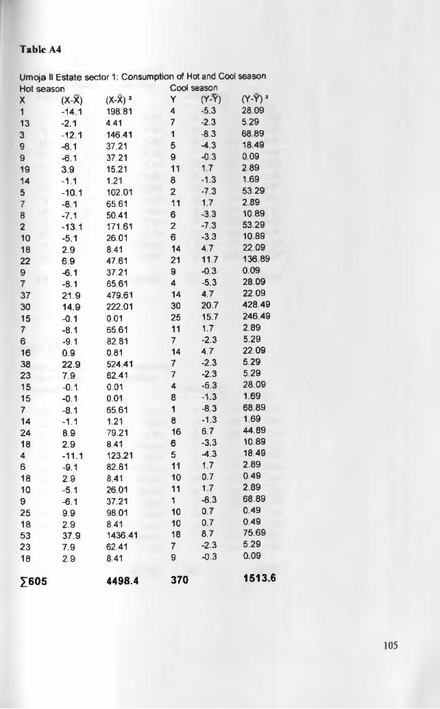
Table A4

U m o ja II E s ta te se c to r 1: C o n sum p tion o f Hot and Cool season H o t season C oo l seasonX (X -X ) (X-X) 2 Y (Y-Y) (Y -Y ) 21 -14 .1 1 9 8 8 1 4 -5.3 2 8 0 913 -2.1 4.41 7 -2.3 5.293 -12 .1 146.41 1 -8.3 68 899 -6.1 37.21 5 -4.3 1 8 4 99 -6.1 37.21 9 -0.3 0.0919 3 .9 15.21 11 1.7 2.8914 -1.1 1.21 8 -1.3 1.695 -10 .1 102.01 2 -7.3 53 .297 -8.1 65.61 11 1.7 2 8 98 -7.1 50.41 6 -3.3 10.892 -13 .1 171.61 2 -7.3 53 .2910 -5.1 26.01 6 -3.3 10.8918 2 .9 8.41 14 4.7 22 .0922 6 .9 47.61 21 11.7 136.899 -6.1 37.21 9 -0.3 0 .097 -8.1 65.61 4 -5.3 28 0937 2 1 .9 479.61 14 4.7 22 .0930 14.9 222.01 30 20.7 4 2 8 .4 915 -0.1 0.01 25 15.7 246 .4 97 -8.1 65.61 11 1.7 2 .896 -9.1 82.81 7 -2.3 5 .2916 0 .9 0.81 14 4 .7 22 .0938 2 2 .9 524.41 7 -2 .3 5 .292 3 7 .9 62.41 7 -2.3 5 .2915 -0.1 0.01 4 -5.3 28 .0915 -0.1 0.01 8 -1.3 1.697 -8.1 65.61 1 -8.3 68 8914 -1.1 1.21 8 -1.3 1.6924 8 .9 79.21 16 6.7 4 4 .8918 2 .9 8.41 6 -3 .3 10.894 -11 .1 123.21 5 -4.3 18.496 -9.1 82.81 11 1.7 2 .8918 2 .9 8.41 10 0.7 0 .4910 -5.1 26.01 11 1.7 2 .899 -6.1 37.21 1 -8 .3 68 892 5 9 .9 98.01 10 0.7 0 .4918 2 .9 8.41 10 0.7 0 .4953 3 7 .9 1436.41 18 8.7 75 .692 3 7 .9 62.41 7 -2 .3 5 .2918 2 .9 8.41 9 -0.3 0 .0 9

1605 4498.4 370 1513.6

105

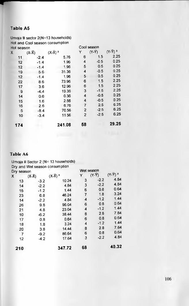
Table A5

U m o ja II sec to r 2 (N = 1 3 households)Hot a n d C oo l se aso n consum ptionHot s e a so n C oo l season

(X-X) (X-X) 2 Y (Y-?) (Y- ? ) 211 -2 .4 5.76 6 1.5 2 2 512 -1 .4 1.96 4 -0.5 0 2512 -1 .4 1.96 5 0.5 0.2519 5 .6 31.36 4 -0.5 0.2512 -1 .4 1.96 5 0.5 0.2522 8 .6 73.96 6 1.5 2.2517 3 .6 12.96 6 1.5 2.25

9 -4 .4 19.36 3 -1 .5 2.2514 0 .6 0.36 4 -0.5 0.2515 1 .6 2.56 4 -0.5 0.2516 2 .6 6.76 7 2.5 6 .25

5 -8 .4 70.56 2 -2.5 6 .25

10 -3 .4 11.56 2 -2 .5 6 .25

174 241.08 58 29.25

Table A6

U m o ja II S e cto r 2 (N = 13 househo lds) D ry a n d W e t se aso n consum ptionD ry season W e t seasonX (X-X) (X-X) 2 Y (Y-Y) (Y-Y) 2

13 -3 .2 10.24 3 -2.2 4 84

14 -2 .2 4.84 3 -2.2 4 .84

15 -1 .2 1.44 6 0.8 0 .64

23 6 .8 46.24 7 1.8 3.24

14 -2 .2 4.84 4 -1.2 1.44

26 9 .8 96.04 6 0.8 0 .64

21 4 .8 23.04 4 -1.2 1.44

10 -6 .2 38.44 8 2.8 7.84

17 0 .8 0.64 6 0.8 0 .64

18 1.8 3.24 4 -1.2 1.44

20 3 .8 14.44 8 2 8 7.84

7 -9 .2 86.64 6 0.8 0 .64

12 -4 .2 17.64 3 -2.2 4 84

210 347.72 68 40.32

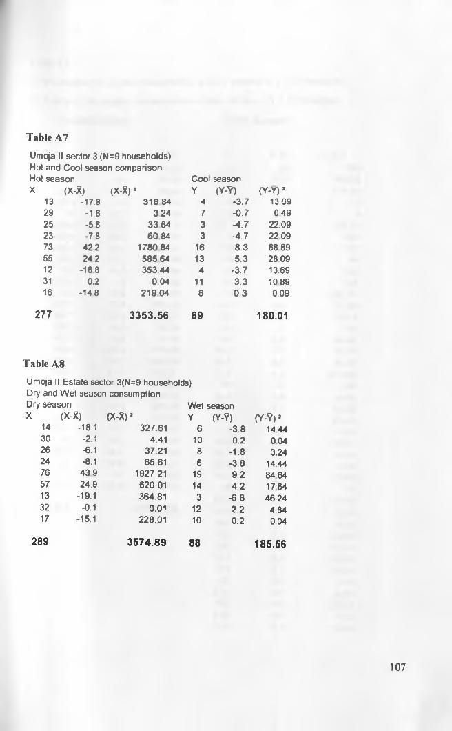
Table A7

U m oja II sec to r 3 (N = 9 h ouseho lds )Hot and C oo l season com p a riso nHot season C oo l seasonX (X -* ) (X -X )* Y (Y -Y ) (Y -Y ) *

13 -17.8 3 1 6 84 4 -3 .7 13.6929 -1.8 3 2 4 7 -0 .7 0 4 925 -5 8 3 3 64 3 -4 .7 22.0923 -7 8 6 0 84 3 -4 .7 22 0973 4 2 2 1780 84 16 8 .3 6 8 8 955 2 4 2 5 8 5 64 13 5 .3 28 0912 -1 8 8 353 .4 4 4 -3 .7 13.6931 0.2 0 .04 11 3 .3 1 0 8 916 -1 4 8 2 1 9 0 4 8 0 .3 0.09

277 3353.56 69 180.01

T a b le A 8

U m oja II E s ta te sector 3 (N=9 househo lds)D ry and W e t season co nsu m ptio nD ry season W et seasonX (X -X ) (X -X )* Y (Y-Y) (Y-Y)*

14 -18.1 327 .61 6 -3 .8 1 4 4 430 -2.1 4.41 10 0 .2 0 0 426 -6.1 37.21 8 -1 .8 3.2424 -8.1 65.61 6 -3 .8 1 4 4 476 4 3 9 1927.21 19 9 .2 84 6457 24.9 620 .01 14 4 .2 1 7 6 413 -19.1 364 .81 3 -6 .8 46.2432 -0.1 0.01 12 2 2 4.8417 -15.1 228 .01 10 0 .2 0.04

289 3574.89 88 185.56

107

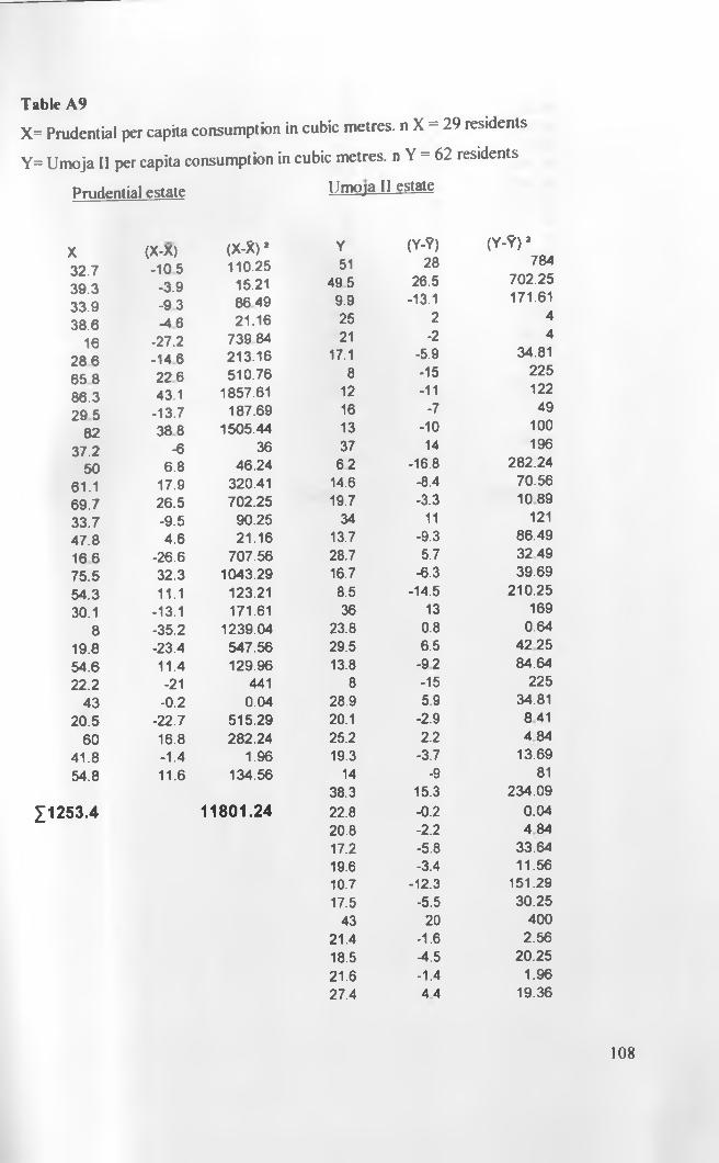
T a b ic A 9X= Prudential per capita consumption in cubic metres, n X = 29 residents

Y= Umoja 11 per capita consumption in cubic metres, n Y = 62 residents

Prudential estate IJmoja 11 estate

X (X -X ) (X -X ) * Y (Y -?) ( Y - ? ) 1

3 2 .7 -1 0 5 110 .25 51 28 784

3 9 .3 -3 .9 15.21 49 5 26.5 7 0 2 .2 5

3 3 .9 - 9 3 86 49 9.9 -13.1 171.61

3 8 .6 - 4 6 2 1 .16 25 2 4

16 -27 .2 739 84 21 -2 4

2 8 6 6 5 8

-14 6 2 2 6

2 1 3 .1 65 1 0 .7 6

17.18

-5.9-15

34.81225

8 6 .3 43.1 1857.61 12 -11 122

2 9 5 82

-13 .7 38 8

187 .691505 .44

1613

-7-10

49100

37.2 -6 36 37 14 196

50 6 .8 4 6 .24 6 2 -16.8 2 8 2 .2 4

61.1 17.9 320.41 14.6 -8.4 7 0 .566 9 .7 26 .5 7 0 2 .2 5 19.7 -3.3 10 893 3 .7 -9 .5 9 0 .25 34 11 1214 7 .8 4 .6 2 1 .16 13.7 -9.3 8 6 .491 6 6 -26 .6 7 0 7 .5 6 28.7 5.7 3 2 4 97 5 .5 32 .3 104 3 .2 9 16.7 -6.3 3 9 .695 4 .3 11.1 123.21 8.5 -14.5 2 1 0 .2 530.1 -13.1 171.61 36 13 169

8 -35 .2 1 239 .04 23.8 0.8 0.6419 .8 -23.4 5 4 7 .5 6 29.5 6.5 4 2 255 4 .6 11.4 129 .96 13.8 -9 2 84 .642 2 .2 -21 441 8 -15 225

4 3 -0 .2 0 .04 28.9 5.9 34.812 0 .5 -22 .7 5 1 5 .2 9 20.1 -2.9 8 4 1

6 0 16.8 2 8 2 .2 4 25.2 2.2 4 844 1 .8 -1 .4 1.96 19.3 -3.7 13.6954.8 11.6 134 .56 14 -9 81

38.3 15.3 2 3 4 .0 9£ 1 2 5 3 . 4 1 1 8 0 1 . 2 4 22.8 -0.2 0 .0 4

20.8 -2.2 4 8417.2 -5.8 33 .6419.6 -3.4 11 .5610.7 -12.3 151 .2917.5 -5.5 3 0 .25

43 20 4 0021.4 -1.6 2 .5 618.5 -4.5 2 0 .2 521.6 -1.4 1.9627.4 4 4 19.36

108

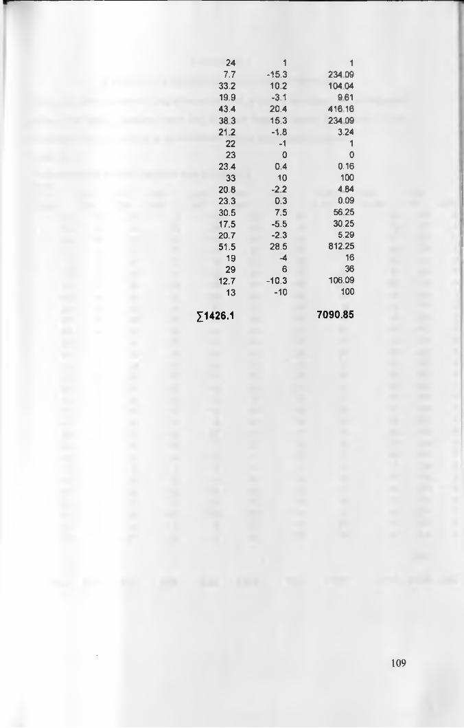
r

24 1 17.7 -15 .3 234 09

33.2 10.2 104 0419.9 -3.1 96143.4 20.4 416 1638 3 15.3 234 0921.2 -1 .8 3.24

22 -1 123 0 0

23.4 0.4 0.1633 10 100

20.8 -2 .2 4 8423.3 0 .3 0.0930.5 7.5 56.2517.5 -5 .5 30.2520.7 -2 .3 5.2951.5 28.5 812.25

19 -4 1629 6 36

12.7 -10 .3 106.0913 -10 100

£1426.1 7090.85

109

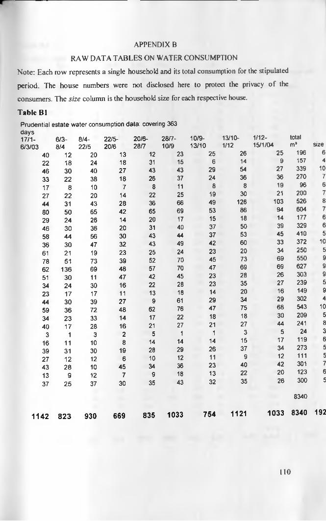
APPENDIX B

RAW DATA TABLES ON WATER CONSUMPTION

Note: Each row represents a single household and its total consumption for the stipulated

period. The house numbers were not disclosed here to protect the privacy o f the

consumers. The size column is the household size for each respective house.

Table B1P ru d e n tia l e s ta te w a te r consum ption d a ta : covering 363days17 /1 - 6 /3 - 8 /4 - 22/5- 20/6- 28/7- 10/9- 13/10- 1/12- total6 /3 /0 3 8 /4 22/5 20/6 28/7 10/9 13/10 1/12 15/1/04 m* size

40 12 20 13 12 23 25 26 25 196 6

22 18 24 18 31 15 6 14 9 157 4

46 30 40 27 43 43 29 54 27 339 10

33 22 38 18 26 37 24 36 36 270 7

17 8 10 7 8 11 8 8 19 96 6

27 2 2 20 14 22 25 19 30 21 200 7

44 31 43 28 36 66 49 126 103 526 8

80 50 65 42 65 69 53 86 94 604 7

29 24 26 14 20 17 15 18 14 177 6

46 30 36 20 31 40 37 50 39 329 6

58 4 4 56 30 43 44 37 53 45 410 5

36 30 47 32 43 49 42 60 33 372 10

61 21 19 23 25 24 23 20 34 250 5

78 51 73 39 52 70 45 73 69 550 9

62 136 69 48 57 70 47 69 69 627 9

51 30 11 47 42 45 23 28 26 303 9

34 2 4 30 16 22 28 23 35 27 239 5

23 17 17 11 13 18 14 20 16 149 9

44 30 39 27 9 61 29 34 29 302 4

59 36 72 48 62 76 47 75 68 543 10

34 2 3 33 14 17 22 18 18 30 209 5

40 17 28 16 21 27 21 27 44 241 8

3 1 3 2 5 1 1 3 5 24 3

16 11 10 8 14 14 14 15 17 119 6

39 31 30 19 28 29 26 37 34 273 5

27 12 12 6 10 12 11 9 12 111 5

43 2 8 10 45 34 36 23 40 42 301 7

13 9 12 7 9 18 13 22 20 123 6

37 2 5 37 30 35 43 32 35 26 300 5

1142 823 930 669 835 1033 754 1121 1033

8340

8340 192

110

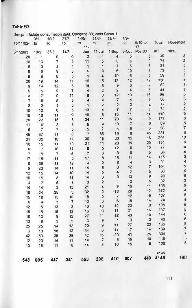
Table B2U m oja II Estate co nsu m p tio n data: C o ve ring 366 days Sector 1

3 /1 - 19/2- 27 /3 - 14 /5- 11/6- 11/7- 1/9-16/11 /02- to to to to

11-3 /1 /2003 19/2 2 7 /3 14/5 Jun

20 1 0 0 210 13 7 5 11

8 3 3 4 19 9 9 8 68 9 6 5 6

20 19 14 11 169 14 12 5 145 5 9 7 43 7 9 11 97 8 6 5 42 2 1 3 1

10 10 8 5 1318 18 11 9 1529 2 2 15 8 3411 9 8 8 66 7 7 5 5

45 37 31 8 731 30 18 11 3016 15 11 10 216 7 10 11 87 6 7 5 7

17 16 11 5 179 38 11 12 49 2 3 14 11 14

12 15 14 10 1416 15 8 11 14

4 7 5 3 314 14 3 13 2118 24 25 5 3215 18 15 10 16

6 4 3 7 1212 6 13 8 1615 18 18 13 1610 10 9 12 2713 9 3 5 325 2 5 14 12 20

6 18 18 13 3442 53 36 28 4212 2 3 14 11 1413 18 11 8 14

548 605 447 341 553

to to to 6/10-to T o ta l Household17

11-Jul 1-Sep 6-O ct Nov 03 m * size4 4 5 3 39 35 8 6 9 74 21 1 5 5 31 59 6 10 7 73 54 10 6 5 59 3

15 12 12 17 136 46 9 6 7 82 62 2 4 6 44 26 12 13 16 86 34 7 4 5 50 32 2 2 2 17 24 7 7 8 72 28 15 11 14 119 5

11 23 16 19 177 64 10 7 6 69 57 4 9 6 56 7

35 15 8 45 231 815 33 15 18 201 1011 28 19 20 151 6

5 12 8 10 77 4

6 8 5 5 56 48 16 11 14 115 32 8 4 3 91 46 8 12 7 104 55 4 7 5 86 53 9 13 9 98 52 1 2 5 32 34 9 16 11 105 6

9 18 29 12 172 4

5 7 12 9 107 56 6 16 14 74 4

10 12 23 8 108 59 11 21 16 137 5

11 12 43 10 144 6

6 1 3 3 46 6

9 11 27 23 166 5

8 11 17 14 139 7

16 20 41 26 304 7

7 8 16 10 115 3

8 10 16 8 106 5

4 149298 410 507 440 4149 1 8 8

111

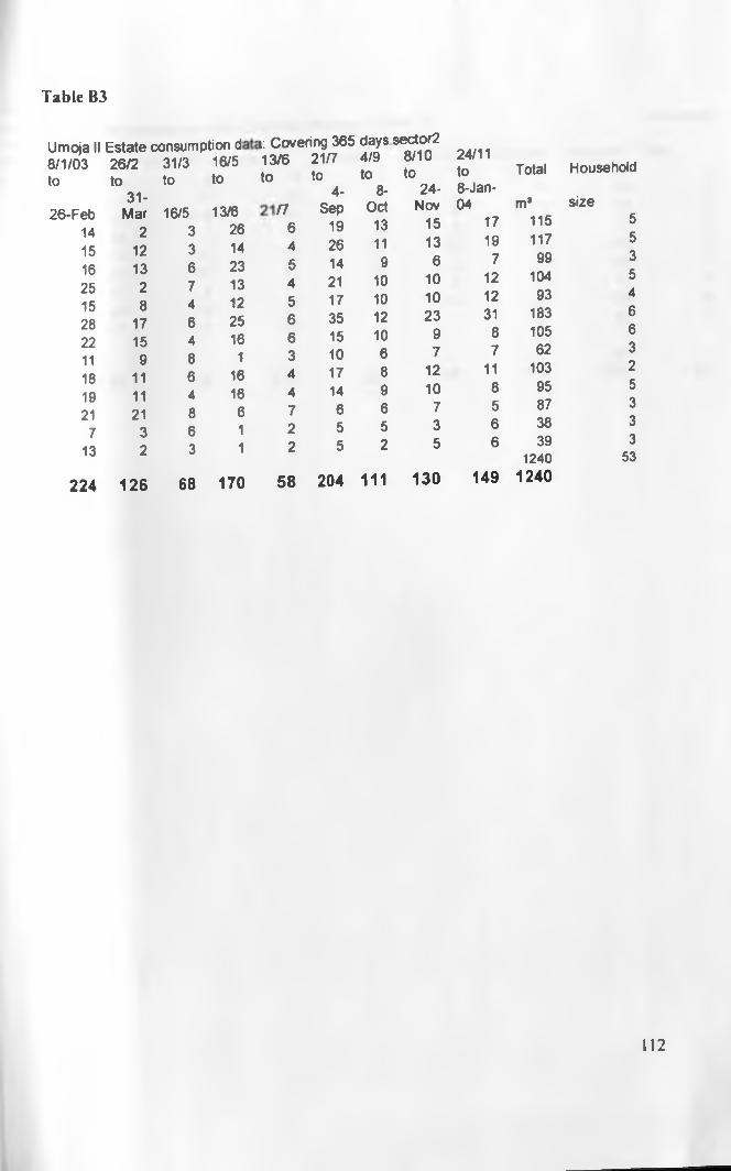
Table B3

U m o ja II E s ta te consum ption d 8 /1 /0 3 2 6 /2 31/3 16/5to to to to

26 -F eb3 1 -

M ar 16/5 13/614 2 3 2615 12 3 1416 13 6 2325 2 7 1315 8 4 1228 17 6 2522 15 4 1611 9 8 118 11 6 1619 11 4 1621 21 8 6

7 3 6 113 2 3 1

224 126 68 170

i: C ove ring 365 days secto r2 13 /6 21/7 4 /9 8 /10to to to to

4- 8- 24-n Sep O ct Nov

6 19 13 154 26 11 135 14 9 64 21 10 105 17 10 106 35 12 236 15 10 93 10 6 74 17 8 124 14 9 107 6 6 72 5 5 32 5 2 5

58 204 111 130

24/11to Tota l H ouseho ld8-Jan-04 m* s ize

17 115 519 117 5

7 99 312 104 512 93 431 183 6

8 105 67 62 3

11 103 28 95 55 87 36 38 36 39 3

1491240

124053

112

Householdble B4io ja II H o u seh o ld s co n su m p tio n data : cove ring 366 days. (Sector 3) 0 -/0 3 8 /1 -28 /2 2 8 /2 -3 1 /3 31 /3 -12 /6 12/6-17/7 17/7-4/9 4/9-7/10/03 total in m * size

5 14 9 9 3 4 7 51 111 30 11 15 7 7 18 99 213 26 8 11 5 3 3 69 731 24 1 9 5 3 2 75 32 4 76 21 27 13 16 33 210 102 7 57 21 20 12 13 4 154 9

5 13 4 5 3 4 6 40 515 32 13 17 8 11 24 120 10

9 17 11 14 7 8 14 80 5

898140 289 99 127 63 69 111 898 52

113

NAIROBI CLIMATIC DATA

JOMO KENYATTA METEOROLOGICAL STATIONLATITUDE: 0 1 1 9 ’ SOUTH

LONGITUDE: 36 55’EASTALTITUDE: 5329 FEET

1624 METRES

Temperature

2002 MAX MIN

JULY 24.3 11.3

AUGUST 22.9 12.9

SEPTEMBER 26.0 12.8

OCTOBER 26.8 14.3

NOVEMBER 25.5 15.5

DECEMBER 25.1 15.3

JANUARY 26.5 13.9

2003

FEBRUARY 28.2 13.4

MARCH 30.1 14.7

APRIL 28.0 15.7

MAY 24.3 15.2

JUNE 23.2 13.1

JULY 22.4 11.6

AUGUST 23.4 11.9

SEPTEMBER 25.2 13.4

OCTOBER 27.0 14.4

NOVEMBER 24.9 15.2

DECEMBER 25.9 14.1

JANUARY 2004 27.4 14.8

Rainfall

AVERAGE TOTAL RAIN

(mm)

17.8 0.2

17.9 3.9

19.4 54.5

20.6 48.7

20.5 115.1

20.2 331.2

20.2 16.9

20.8 9.5

22.4 22.1

21.9 154.6

19.7 229.8

18.1 6.8

17.0 1.6

17.5 47.8

19.3 40.8

20.7 52.3

20.1 119.8

20.0 25.2

21.1 95.3

114

Q U ESTION NA IRET h is research concerns the w ater consum ption o f households in N airob i.Y our answ ers will be useful in planning fo r future w ater provision.Please answ er th e follow ing questions as accurately as possible.

1. H ouse N u m b er___________

2. W hat nam e a p p e a rs on y o u r w a te r bill_____________________________

3. How long has y o u r family lived in th is house(Tick one below)

F o r m ore th an two years ________

F o r less th a n two years ________

4. How m any people usually live in y o u r house (Including those w ho may be in b o a rd in g schools,etc)

5. Has this usual number of residents been the same since 2002 (tick one)Yes______ No______

6. Among the methods given below, which one do you often use to take a bath (tick one)

a) A basin/ bucket _______

b) A Shower _______

c) A bathtub _______

7. Do you usually drink water directly from the tap without boiling it first ? (tickone)

Yes______ No______

8. Given the choices below,how would you describe the costs of your water bills? (tick one)

a) Expensive______

b) Fair ______

c) Cheap ______

9. Given the two choices below,what problem would you like the Nairobi Water and Sewerage Company to solve first? ( tick one)

a) Improve water quality _______

b) Reduce w ater shortages_____

T h a n k you very M uch.115

, a fi-n m TCF (Totally chlorine free) pulp.85% of water used in producing 'the^paper"^^ recycled. Wood chained from fore,, under suaainabie

management.UNI VERSI TY OF NAIROBIEAST AF klCANA COLLECTION

liM l i A MLMLlrWUBPAM

v J

Domestic Water Consumption Per Capita: A Case Study Of ...

Documents

Transcript of Domestic Water Consumption Per Capita: A Case Study Of ...