Does Reject Inference Really Improve the Performance of

Edinburgh Research Explorer

Does reject inference really improve the performance ofapplication scoring models?

Citation for published version:Banasik, J & Crook, J 2004, 'Does reject inference really improve the performance of application scoringmodels?', Journal of Banking and Finance, vol. 28, pp. 857-874.https://doi.org/10.1016/j.jbankfin.2003.10.010

Digital Object Identifier (DOI):10.1016/j.jbankfin.2003.10.010

Link:Link to publication record in Edinburgh Research Explorer

Document Version:Peer reviewed version

Published In:Journal of Banking and Finance

Publisher Rights Statement:Banasik, J., & Crook, J. (2004). Does reject inference really improve the performance of application scoringmodels?. Journal of Banking & Finance, 28, 857-874doi: 10.1016/j.jbankfin.2003.10.010

General rightsCopyright for the publications made accessible via the Edinburgh Research Explorer is retained by the author(s)and / or other copyright owners and it is a condition of accessing these publications that users recognise andabide by the legal requirements associated with these rights.

Take down policyThe University of Edinburgh has made every reasonable effort to ensure that Edinburgh Research Explorercontent complies with UK legislation. If you believe that the public display of this file breaches copyright pleasecontact [email protected] providing details, and we will remove access to the work immediately andinvestigate your claim.

Download date: 29. Dec. 2021

https://doi.org/10.1016/j.jbankfin.2003.10.010

https://doi.org/10.1016/j.jbankfin.2003.10.010

https://www.research.ed.ac.uk/en/publications/ef4b8e89-67bd-43f4-9dd7-d942313e291f

Does Reject Inference Really Improve the Performance of Application Scoring Models?

by

Jonathan Crook and John Banasik

Working Paper Series No. 02/3

ISBN 1 902850 61 11

Does Reject Inference Really Improve the Performance of Application Scoring Models?

Jonathan Crook* and John Banasik

Credit Research Centre, The School of Management, University of Edinburgh, 50 George Square, Edinburgh EH8 9JY.

* Corresponding author: J Crook, Credit Research Centre, School of Management, University of Edinburgh, 50 George Square, Edinburgh EH8 9JY [email protected] Tel: (+44) 0131 650 3802

1

Introduction

Application credit scoring is the process of predicting the probability that an applicant

for a credit product will fail to repay the loan in an agreed manner. To assess this

process we require a model which represents the behaviour of all applicants for credit,

yet typically we have only information about the repayment behaviour of those who

have been accepted (and booked) for credit in the past. The behaviour of those who

had been rejected, if they had been accepted, is unknown. If one estimates a model

using accepted applicants only one may gain biased parameters, if those parameters

are taken to apply to a model representing the behaviour of all applicants. In addition,

if cut-offs are chosen to equalise the actual and predicted number of bads then a

sample of accept-only is likely to yield inappropriate cut-offs for the population of all

applicants.

Several techniques for reducing the magnitude of the bias have been proposed either

in the literature or by consultancies. These include extrapolation, augmentation (Hsai

1979), iterative reclassification (Joanes 1993), bivariate probit (Boyes 1989)

"parcelling", use of the EM algorithm, (Demster, 1977) using a multinomial logistic

model, (Reichert and Choi 1983), and collecting repayment performance data for

rejects (Hand & Henley 1993, Ash and Meester, 2002). The necessary assumptions

for the use of these techniques and their plausibility when made about data typically

used in credit scoring models have been reviewed by a number of authors (Ash &

Meester 2002, Banasik et al 2001, Hand & Henley 1993, Joanes 1993, Thomas,

Edelman, and Crook 2002). Relatively little has been published which empirically

compares the predictive performance of algorithms, which incorporate different

possible reject inference techniques. Two methods of extrapolation were considered

by Meester (2000). These were firstly a model built on accepted cases only, with the

2

performance of rejected cases imputed from the accept-only model, and secondly, a

model built on the accepted and rejected cases where the performance of the rejects

had been imputed from a model estimated for the accepts and given a cut-off.

Meester found that for a revolving credit product, up until the 50th percentile score the

imputed model was marginally inferior to the extrapolated model estimated for

accepts only, which in turn was inferior to a model based on a sample where the

performance of all cases was known. When applied to data for an instalment credit

product the imputed model performed better than the accept-only model, but was

inferior to the full sample model.

In the case of the bivariate probit, Banasik et al (2001) found that this modelling

approach gave minimal improvement in predictive performance compared with a

model based on accept-only. Finally, acquiring credit bureau data on how rejected

applicants performed on loans they were granted from other suppliers, and imputing

the probability that each rejected applicant would default, given this information, is

proposed by Ash & Meester (2002). Using a sample of business leases they found at

each approval rate the proportion of cases classed as bad was considerably closer to

the actual proportion than if no reject inference had been used, that is, an accept-only

model was employed.

However, there is no published empirical evaluation of the predictive performance of

the reject inference technique that is perhaps the most frequently used, augmentation

(or re-weighting). The aim of this paper is to report such an evaluation and to

compare its performance with extrapolation. In the next section we explain the

technique in more detail. In the following sections we explain our methodology and

results. The final section concludes.

3

Re-weighting

Although there are several variants of re-weighting, the basic method is as follows

(see Table 1). First an accept-reject (AR) model is estimated using cases which have

been accepted or rejected over a given period of time by the current model. If the

model has been applied without over-rides, if the explanatory variables within it are

known (call them Xold) and if the algorithm used, functional form of the model and all

other parameters of the original estimation process are known, then this model can be

estimated perfectly. Otherwise it cannot be estimated perfectly. The scores predicted

by the AR model are banded and within each band, j, the numbers of rejected Rj and

accepted Aj cases are found. For each Aj there are gj good cases and bj bad cases

Table 1: Re-weighting

Number of Number of Number of Number of Band Band (j) of Goods of Bads Accepts Rejects Weight

1 g1 b1 A1 = g1 + b1 R1 (R1 + A1) / A1 2 g2 b2 A2 = g2 + b2 R2 (R2 + A2) / A2 . . . . . .. . . . . .. . . . . .. . . . . .. . . . . .n gn bn An = gn + bn Rn (Rn + An) / An

Assuming

P(g | Sj, A) = P(g | Sj , R) …...(1)

then

jrjjj RgAg =

where rjg is the imputed number of goods amongst the rejects within band j;

jrj Rg is the proportion of rejects in band j which would have been good, had

they been accepted.

4

Therefore the Aj accepts in band j are weighted to represent the Aj and Rj cases in the

band and each Aj is weighted by (Rj + Aj)/Aj. This is the inverse of the probability of

acceptance in band j and is the probability sampling weight for band j.

Since accepted scores are monotonically related to the probability of being accepted

we can replace scores by these probabilities, and if instead of bands we consider

individual values, where there are m possible values (because there are m cases), each

row relates to P(Ai) i=1…m. Thus each accepted case has a probability sampling

weight of 1/P(Ai). A good-bad model using the weighted accepts is then estimated.

The re-weighting method has been criticised by Hand & Henley (1993 & 1994) who

build on the work of Little & Rubin (1987). To explain the criticism we define Xnew

to be the vector of explanatory variables used to model good-bad repayment

performance to yield the model, which will replace the original model. The original

model had a vector of explanatory variables Xold. Hand and Henley argue that if Xold

is not a subset of Xnew then the assumption of equation (1) will result in biased

estimates of the probability of default. To understand this let

D = (1,0) indicate whether a case has defaulted or not . This can be partitioned

into Do and Dm where subscript o indicating this value is observed, and

subscript m indicating the value is missing

A = (1,0) indicate whether D is observed (in the case of previously accepted

applicants) or missing (in the case of previously rejected applicants).

We can write

P(D = 1 | Xnew) = P(D = 1 | A = 1, Xnew).P(A = 1 | Xnew)

+ P(D = 1 | A = 0, Xnew).P(A = 0 | Xnew) …...(2)

If P(A) depends only on Xnew then P(D | A = 1, Xnew) = P(D = 1 | A = 0, Xnew) so

equation (2) becomes

5

P(D = 1 | Xnew) = P(D = 1 | A = 1, Xnew) ……(3)

However, if P(D = 1 | A = 1, Xnew) ≠ P(D = 1 | A = 0, Xnew ) then equation (3) will

not hold and this will result in biased estimates. Put simply, if there are variables in

Xold which are not in Xnew , call them Xadded , but which cause P(D = 1 | A, Xnew) to

vary, then in general P(D = 1 | A = 1, Xnew) ≠ P(D = 1 | A = 0, Xnew). For equation (3)

to hold, Xnew must include Xold variables so there are no variables which could cause

P(D = 1 | A, Xnew) to vary; all variables affecting this probability are included in Xnew.

Hand and Henley (1994) and Banasik et al (2001) show that if Xold is not a subset of

Xnew then we have a case of Little and Rubin's non-ignorably missing mechanism

where A depends on Xnew and on Xadded , that is variables which are in Xold but not in

Xnew. These Xadded variables affect D and so A depends on D and Xnew, which is

exactly Little and Rubin's definition of the non-ignorably missing mechanism. Since

values of D depend on the probability they are observed, P(A=1), and this depends on

Xold and Xadded, the omission of Xadded from the likelihood of the parameters of the D

function will result in omitted variable bias in the estimated parameters.

So far we have assumed that the same parameters apply to the P(D | A = 1, Xnew)

model as to the P(D | A = 0, Xnew) model. If this is false then we must establish

separate models for the accepts and for the rejects.

Extrapolation

As with re-weighting there are several methods of extrapolation. The method we

consider is to estimate a posterior probability model using accept-only data,

extrapolate the probability of default for the rejected cases and by applying a cut-off

probability classify the rejected cases as either good or bad. A new good-bad model

is then estimated for all cases (See Ash and Meester 2002).

6

If the regression coefficients of the good-bad model which are applicable to the

accepts also apply to the rejects then this procedure would have minimal effect on the

estimates of these coefficients, although the standard errors of the estimated

coefficients will be understated. However, if variables other than Xnew affect the

probability of acceptance we again have the case of non-ignorably missing

observations. Again, equation (3) would not hold and extrapolation would yield

biased estimates of the posterior probabilities.

If Xold is a subset of Xnew and equation (3) does hold (we have Little and Rubin’s

“missing at random” case) a further source of error in the predicted probabilities may

occur due to the proportion of goods and bads in the training sample not being equal

to the proportion in the all-applicant population. This may cause the cut-off

probabilities, which equalise the expected and actual number of bads in the training

sample, to deviate from the cut-offs required to equalise the actual and predicted

number of bads in the all-applicant population. The regression model may give

unbiased posterior probabilities, but applicants would be misallocated because

inappropriate cut-offs may be applied.

Methodology

Few credit granters ever give credit to all applicants because of the potential losses

from those with a high probability of default. However, we do have a sample of all

applicants for a credit product, rather than of merely accepted applicants, although

certain limitations of it must be acknowledged. The proprietary nature of the data

restricts the details of it that we can describe. To gain this product a customer must

progress through two stages. First a potential applicant must seek information about

the product. Some potential applicants are rejected at this stage and we do not have

7

information about these. We believe that this is a very small proportion of applicants.

Second, those who receive information apply for the product. We have data on these

applicants who applied in a fixed period within 1997. Normally the credit provider

would apply scoring rules to divide this group into accepts and rejects.

A repayment performance is defined to be “bad” if the account was transferred for

debt recovery within 12 months of the credit being first taken. All other accounts

were defined to be “good”. This definition is obviously arbitrary but we believe it is

the best possible given the indivisible nature of the definitions available to us from the

data supplier. We had available the accept-reject decision which the credit grantor

would have implemented for each applicant under normal practice, although for our

sample the indicated decision had not been implemented. This decision was

deterministic – there were no overrides – and was based on an existing statistical

model that had been parameterised from an earlier sample. Call this model 1. A

relatively small subset of the variables which were available to us to build a

replacement model, model 2, were used in this existing model, although almost all the

variables available to build model 1 were available to build model 2. We do not know

any more about the nature of model 1.

In an earlier paper (Banasik et al 2001) we indicated, using the same dataset, that

there was little scope for reject inference to achieve an increase in predictive

performance using the data supplier’s classification of cases into accepts and rejects.

Our first objective in this paper was to examine whether re-weighting would improve

the performance of an unweighted accept-only model, again using that data provider’s

accept-reject classification. Since use of an accept-only sample rather than a sample

of all applicants may result in an unrepresentative hold-out sample and so erroneous

8

cutoffs compared with those from an all-applicant hold-out, we examine this effect

also. Our second objective was to investigate whether our findings using the data

supplier’s accept-reject classification would apply if different cutoffs were used in the

original reject-accept decision. This required fabrication. Our final objective is to

assess the performance of extrapolation.

To achieve our first objective we built three models using logistic regression. The

first used the re-weighting procedures outlined above. An accept-reject model was

estimated using the data provider’s classification of whom it would have accepted and

whom it would have rejected according to its current model. A good-bad model was

then estimated using the inverse of the probability of acceptance (which was

estimated from the first stage) as probability sampling weights. The second model

was an unweighted good-bad model parameterised only for the accepted cases. The

third model was an unweighted good-bad model parameterised for a sample of all

cases (including those that would have been rejected). The third model yields

parameters which are unbiased by sample selection effects. We used separate weights

of evidence transformations of the explanatory variables for the accept-only sample

and for the sample of all applicants. As an alternative we also used binary variables

to indicate whether a case was within a weight of evidence band for a particular

applicant attribute or not.

The first good-bad model was estimated for a stratified random sample of all accepted

applicants and the initial accept-reject model was estimated for a stratified random

sample of all applicants. The second model was estimated for a stratified random

sample of accepted applicants and the third model for a stratified sample of all

applicants. The performance of each model was assessed by its performance when

9

classifying each of two hold-out samples: a hold-out sample from all applicants and a

hold-out sample from the accept-only. The stratifications preserved the exact

proportions of goods and bads in the hold-out sample for all applicants as in the

population of all applicants.

The measures of performance were the area under the ROC curve (AUROC) and the

percentage of hold-out sample cases correctly classified. For both hold-out samples

we set the cut-off posterior probabilities to equalise the predicted number and actual

number of bads in the training sample and separately in the all-applicant hold-out

sample.

Results using Original Data

Our results when we used the data granter’s classification of cases into accepts and

rejects are shown in Tables 2 to 5. Tables 2 and 3 show the predicted performance

using weights of evidence values and Tables 4 and 5 show the results using binary

variables. We used all of the 46 variables that were available to us.

Table 2: Original Data: Simple Logistic Model with Weights of Evidence

Comparison 1: Area under ROC:

Training Own Band Hold-out All-applicant Hold-out AcceptPredicting Sample Number ROC Number ROC AnalysisModel Cases of Cases Area of Cases Area Delusion

Accepted 5413 2755 .7932 4069 .7818 .0114 All Case 8139 4069 .7837 4069 .7837

Comparison 2: Percentage Correctly Classified:

Own Band Hold-out Prediction All-applicant Hold-out Prediction Own Band Own Band Own Band All Band AcceptPredicting Number Training Hold-out Number Training Hold-out AnalysisModel of Cases Cut-off Cut-off of Cases Cut-off Cut-off Delusion

Accepted 2755 76.19% 75.97% 4069 70.83% 71.74% 5.36%All Case 4069 72.16% 72.13% 4069 72.16% 72.13%

10

Table 3: Original Data: Re-weighted Logistic Model with Weights of Evidence







Consider first the weights of evidence results. We first refer to the results using

AUROC (Comparison 1 in Tables 2 and 3) where the particular issues concerning the

appropriate cutoff do not arise. Four observations can be made. Firstly the scope for

improvement by any reject inference technique is very small. Estimating an

unweighted model for accepted applicants only (Table 2) and testing this on a hold-

out sample of all applicants to indicate its true predicted performance gives an

AUROC of 0.7818 compared to 0.7837 for a model estimated for a sample of all

applicants. Second, establishing an unweighted accept-only model and testing it on

an accept-only hold-out sample overestimated the performance of the model. An

accept-only model tested on an accept-only hold-out gave an AUROC of 0.7932

whereas the performance of the model tested on a sample of all applicants is 0.7818.

Third, using re-weighting as a method of reject inference was found to reduce the

predictive performance of the model compared with an accept-only model; the

AUROC values were 0.7765 (Table 3 Comparison 1) and 0.7818 (Table 2

Comparison 1) respectively. Fourthly, estimating a reweighted model and testing it

on an accept-only model also overestimated the true performance, giving an AUROC

11

of 0.7875 rather than a more representative 0.7765 (Table 3 Comparison 1). All of

these results were also found using binary variables.

The predictive performances using percentages correctly classified are also shown in

Tables 2 and 3 for weights of evidence. First the scope for improvement due to

improved model coefficients is small: from 71.74% to 72.13% (Table 2 Comparison

2). Second, the accept-only model tested on an accept-only hold-out (with training

sample cut-offs) would considerably overestimate the model’s performance: 76.19%

correctly classified compared with 70.83% when tested on an all application sample

(Table 2 Comparison 2). Third the re-weighted model gave a similar performance to

the accept-only model when tested on the all-applicant sample (with the training

sample cut-offs): 71.25% correct (Table 3 Comparison 2) compared with 70.83%

(Table 2 Comparison 2) respectively. Fourthly using an accept-only hold-out with

accept-only cut-offs considerably over emphasises the performance of the reweighted

model compared with a hold-out of all applications: 75.97% correct compared with

71.34% respectively (Table 3 Comparison 2). Again these results were also found

using binary variables.

Table 4: Original Data: Simple Logistic Model with Binary Variables







12

Table 5: Original Data: Re-weighted Logistic Model with Binary Variables







Banded Analysis

We did not have access to the original accept-reject model used by the data supplier

nor to the data from which it was estimated. In order to investigate the extent to

which similar results would arise were we to vary the cut-offs for an accept-reject

model, a new accept-reject model had to be constructed. Knowledge of the basis for

applicant acceptance by this new model permits as well the character of our reject

inference results to be better understood. The new model required some of the data

set, the 2540 Scottish cases, to be dedicated to the accept-reject model and the rest,

the 9668 English and Welsh (hereafter English) cases, to be dedicated to the good-bad

models. The variables used to build each of these two types of model differed by an

arbitrary selection such that each model had some variables denied the other.

Typically, the accept/reject distinction would arise from a previous and perhaps

somewhat obsolete credit-scoring model that distinguished good applicants from bad.

It may also to some extent reflect some over-riding of credit scores by those using

such a model. In setting up Scottish accept/reject and English good/bad models, the

national difference in the data used for the two models appear as a metaphor for the

13

inter-temporal difference that would separate the observations used to build two

successive models. The exclusion of some Scottish variables in the development of

the English model may be considered to represent, in part, the process of over-riding

the acceptance criteria provided by the Scottish model. The exclusion of some

English variables in the development of the Scottish model represents the natural

tendency of new models to incorporate new variables not previously available. The

progress of time also facilitates the incorporation of more variables by providing more

cases and thereby permitting more variables to enter significantly.

The variable selection for the English and Scottish models was designed to retain

some of the flavour of the original performance and acceptance models. An eligible

pool of variables for the accept-reject model, to be parameterised on Scottish data,

was identified by three stepwise (backward Wald) regressions using Scottish, English,

and UK cases, where accept-reject was the dependent variable. An explanatory

variable that survived in any one of the three equations was deemed to have possibly

influenced the acceptance by the data supplier. The eligible variables were then used

to model good-bad behaviour in Scotland in a backward stepwise procedure that

eliminated further variables.

Determination of the variable set for the good-bad model, to be parameterised on

English data, arose from a backward stepwise regression using English data, starting

with all variables available to the English cases. A few scarcely significant variables

common to the English and Scottish variable sets were then eliminated from one or

the other to increase the distinctiveness of the two regressor lists. The resulting

variable selections are shown in Table 6.

14

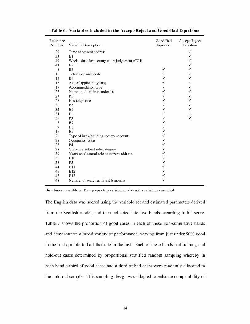
Table 6: Variables Included in the Accept-Reject and Good-Bad Equations

Reference Good-Bad Accept-Reject Number Variable Description Equation Equation

20 Time at present address 33 B1 40 Weeks since last county court judgement (CCJ) 43 B2

6 B3 11 Television area code 15 B4 17 Age of applicant (years) 19 Accommodation type 22 Number of children under 16 23 P1 26 Has telephone 31 P2 32 B5 34 B6 35 P3

7 B7 9 B8

16 B9 21 Type of bank/building society accounts 25 Occupation code 27 P4 28 Current electoral role category 30 Years on electoral role at current address 36 B10 38 P5 44 B11 46 B12 47 B13 48 Number of searches in last 6 months

Bn = bureau variable n; Pn = proprietary variable n; denotes variable is included

The English data was scored using the variable set and estimated parameters derived

from the Scottish model, and then collected into five bands according to his score.

Table 7 shows the proportion of good cases in each of these non-cumulative bands

and demonstrates a broad variety of performance, varying from just under 90% good

in the first quintile to half that rate in the last. Each of these bands had training and

hold-out cases determined by proportional stratified random sampling whereby in

each band a third of good cases and a third of bad cases were randomly allocated to

the hold-out sample. This sampling design was adopted to enhance comparability of

15

corresponding hold-out and training cases and to retain the pattern of behaviour in

successive bands.

Finally, the bands were cumulated with each band including the cases of those bands

previously above it. These are the bands used in subsequent analysis. Each band

represents a possible placement of an acceptance threshold with the last representing a

situation where all applicants are accepted. In the tables showing banded results, that

last band is one where the opportunity for reject inference does not arise. It appears in

tables that show results from reject-inference as a limiting case where no rejected

cases are available to be deployed.

Table 7: Sample Accounting

Cases Not Cumulated into English Acceptance Threshold Bands to Show Good Rate Variety:

All Sample Case Good Training Sample Cases Hold-out Sample Cases Good Bad Total Rate Good Bad Total Good Bad Total

Band 1 1725 209 1934 89.2% 1150 139 1289 575 70 645Band 2 1558 375 1933 80.6% 1039 250 1289 519 125 644Band 3 1267 667 1934 65.5% 844 445 1289 423 222 645Band 4 1021 912 1933 52.8% 681 608 1289 340 304 644Band 5 868 1066 1934 44.9% 579 711 1290 289 355 644

English 6439 3229 9668 66.6% 4293 2153 6446 2146 1076 3222Scottish 1543 997 2540 60.7%

Total 7982 4226 12208 65.4%

Cases Cumulated into English Acceptance Threshold Bands for Analysis:

English Sample Cases Good Training Sample Cases Hold-out Sample Cases Good Bad Total Rate Good Bad Total Good Bad Total

Band 1 1725 209 1934 89.2% 1150 139 1289 575 70 645Band 2 3283 584 3867 84.9% 2189 389 2578 1094 195 1289Band 3 4550 1251 5801 78.4% 3033 834 3867 1517 417 1934Band 4 5571 2163 7734 72.0% 3714 1442 5156 1857 721 2578Band 5 6439 3229 9668 66.6% 4293 2153 6446 2146 1076 3222

Coarse categories used for each variable in the various models were those used in the

above analysis of the data originally provided in spite of the fact that the new training

samples were selected for analysis of the banded data, since the original categories

16

seemed quite robust. However, for models involving weights of evidence, separate

weights of evidence were calculated for each variable for each of the five bands.

To explore the extent to which weights of evidence imply constraint that may

influence the scope for reject inference, each experiment has been replicated with a

variable set comprising binary variables corresponding to each coarse category of

each variable

Banded Results

Comparison 1 in Tables 8 and 9 show our results using AUROC as a performance

measure and Comparison 2 in these tables show our results using percentages

correctly classified. These tables show weights of evidence results. The results for

binary variables are shown in Tables 10 and 11. Apart from showing that the scope

for any improvements in performance increased as the cut-off in the original model is

raised, as was shown in an earlier paper, these tables indicate many new findings.

First by comparing Comparison 1 column 6 in Tables 8 and 9 where the hold-out

relates to a sample of all applicants, it can be seen that the use of re-weighting reduces

predicted performance compared with an unweighted model. Furthermore, the

deterioration is greater for bands 1 and 2 than for bands 3 and 4. Generally, it seems

the higher the cut-off score in the original accept-reject model the greater the

deterioration caused by re-weighting.

17

Table 8: Band Analysis: Simple Logistic Model with Weights of Evidence



Band 1 1289 645 .8654 3222 .7821 .0833 Band 2 2578 1289 .8249 3222 .7932 .0317 Band 3 3867 1934 .8175 3222 .8009 .0166 Band 4 5156 2578 .8108 3222 .8039 .0069 Band 5 6446 3222 .8049 3222 .8049



Band 1 645 89.30% 89.77% 3222 70.20% 72.56% 19.10%Band 2 1289 83.40% 83.86% 3222 70.58% 72.75% 12.82%Band 3 1934 79.21% 79.42% 3222 71.97% 73.49% 7.24%Band 4 2578 75.37% 75.56% 3222 72.47% 73.81% 2.90%Band 5 3222 73.65% 73.49% 3222 73.65% 73.49%

Table 9: Band Analysis: Re-weighted Logistic Model with Weights of Evidence



Band 1 1289 645 .8483 3222 .7374 .1109 Band 2 2578 1289 .7509 3222 .7104 .0405 Band 3 3867 1934 .8034 3222 .7920 .0114 Band 4 5156 2578 .8017 3222 .8036 –.0019 Band 5 6446 3222 .8049 3222 .8049




18

Table 10: Band Analysis: Simple Logistic Model with Binary Variables







Table 11: Band Analysis: Re-weighted Logistic Model with Binary Variables







19

Second by comparing the performance when tested on a hold-out from the accept-

only (i.e. for each band separately) with that found when using a hold-out for all

applicants (Comparison 1 in Tables 8 and 9, column 4 with column 6) it can be seen

that the former is overoptimistic in its indicated result. This is true for the unweighted

model and for the model with re-weighting. For example, if the original accept-reject

model had a high cut-off (band 1) and the analyst used these accepts to build and test

a model, the indicated performance would be an AUROC of 0.8654 whereas the

performance on a sample representative of all applicants would be 0.7821 (Table 8

Comparison 1). The difference of 0.0833 is indicative of the error that would be

made and we call this ‘accept analysis delusion’. Values of this delusion are shown in

column 7 in Tables 8 and 9. Notice that the size of the delusion is positively and

monotonically related to the height of the cut-off in the original accept-reject model.

Consistent results are gained when binary variables are used.

Our results using the percentage correctly classified are shown in Comparison 2 of

Tables 8 and 9. Since an analyst would use the hold-out sample merely to test a

model whose parameters (including the cut-off) were calculated from a training

sample, one can see from columns 3 and 6 that the size of the delusion is substantial at

cut-offs which equate expected and actual numbers of bads in the training band. For

example, with a high cut-off (band 1) in the original accept–reject model the delusion

is 19.10% of cases in both the unweighted and weighted models.

Secondly, column 6 of Comparison 2 in each of Tables 8 –11 indicates the modest

scope for improved classification by using information about the good-bad behaviour

of rejected applicants. Each result in that column indicates classification performance

over applicants from all bands when parameters and cut-offs are taken from the

20

particular band. In particular, the cut-off is taken such that predicted and actual

numbers of goods in the training sample are equal. In this way the chosen cut-off

reflects in part the band’s own good-bad ratio, and takes no account of the all-

applicant good-bad ratio. As we move from the low risk Band 1 to the higher risk

bands below it we observe classification performances that approach that which is

possible when no applicant is rejected. In Table 8, for example, the maximum scope

for improved classification is only 3.45% (73.65% – 70.20%). At best reject

inference can but close this gap by producing better regression coefficients and/or by

indication better cut-off points.

Thirdly, column 7 of Comparison 2 in each of Table 8 – 11 suggests a negligible

scope for reject inference to improve classification performance were the population

good-bad rate to be actually known. In that column each band reports classification

where each applicant is scored using regression coefficients arising from estimation in

that band’s training sample. However, the cut-off score is that which will equate the

number of predicted bads among all applicants with the actual number of bads in the

hold-out sample of all applicants. In this way each band’s cut-off is determined by a

good sample-based indication of the good-bad ratio for the whole population of

applicants. As we move from the low risk Band 1 to the higher risk bands below it

we see a maximum scope for improved classification of only .83% (73.49% –

72.56%). Indeed for all but the top two bands there is no scope for improvement at

all. The negative scope for improvement in Band 4 (73.49% – 73.81%) must be seen

as a reflection of sample error and indicates thereby how precariously small is even

the improvement potential for Band 1.

21

Of course, knowledge of the population good-bad ratio required to generated the

results of column 7 in Comparison 2 is unlikely to be available, and so column 6

remains the likely indication to an analyst of the scope for reject inference to improve

classification. However, since the scope for improvement all but vanishes in the

presence of a suitable cut-off point, there seems correspondingly negligible potential

benefit from the removal of bias or inefficiency in the estimation of regression

coefficients used to score the applicants.

Finally, turning to the actual classification performance when re-weighting is used to

attempt improvement in the estimation of regression coefficients, corresponding

elements in column 6 of Comparison 2 of Tables 8 and 9 indicate very small

improvements for Bands 3 and 4 and worse performances in Bands 1 and 2. For

example, in Band 1 the performance of the reweighted model is 69.77% compared

with 70.20% for the unweighted model, yet in Band 4 the corresponding

performances are 72.84% and 72.47%, respectively. An interesting comparison

feature of the re-weighting procedure is shown by comparing Table 8, column 7 with

Table 9 column 7. Table 9 column 7 presents a relatively large scope for improved

performance even in the presence of a suitable cut-off that reflects knowledge of the

population good-bad ratio. The potential for improvement is 4.43% (73.49% -

68.96%). Therefore, while re-weighting undermines predictive performance by a

minimal amount without such knowledge, it appears to undermine ability to deploy

such information. Again these results were found when binary variables were used

instead of weights of evidence.

Extrapolation Results

The foregoing discussion has demonstrated relatively little potential for improved

regression coefficients but indicates considerable scope for using the population good-

22

bad ratio to advantage. Extrapolation is mainly an attempt to obtain a good indication

of that ratio. Rejects are first classified as good or bad by using a good-bad model

parameterised using the training accept-only sample together with cut-offs which

equalise the actual and predicted number of bads in the training sample of a particular

band. These predictions are then combined with the actual good-bad values observed

in the band, and an all-applicant model is calculated. This second model can hardly

be expected to produce very different coefficients, so any scope for improvement will

arise out of the application of a cut-off that reflects the good-bad ratio imputed for the

all-applicant sample.

Table 12 shows that extrapolation gave a virtually identical predictive performance

compared with model estimated only for the accepts. This is roughly true for every

band. With binary variables the results are almost consistently better albeit by a small

amount. With weights of evidence the results seem very slightly worse when using

extrapolation. However, that result might be reversed were the weights of evidence to

be recalibrated using the imputed values of good-bad performance as in principle they

should have been. The small margins of potential benefit indicated provide but a hint

of what further research might indicate.

Table 12: Band Analysis: Extrapolation Percentage Correctly Classified

All-applicant Hold-out Sample using Training Sample Cut-off Points:

Weights of Evidence Predictions Binary Variable Predictions Predicting Number Simple Logistic with Simple Logistic withModel of Cases Logistic Extrapolation Logistic Extrapolation

Band 1 3222 70.20% 69.80% 68.65% 68.56% Band 2 3222 70.58% 70.20% 69.46% 69.58% Band 3 3222 71.97% 71.79% 72.13% 72.35% Band 4 3222 72.47% 72.63% 72.91% 73.34% Band 5 3222 73.65% 73.65% 74.24% 74.24%

23

Conclusion

The analysis of reject inference techniques discussed above benefit from availability

of a data set that permits the results of reject inference to be assessed in light of the

actual repayment performance of “rejected” cases. The data set reflects a situation in

which virtually no applicant was rejected in order for the data supplier to infer the

character of the population of all applicants. The virtual absence of actual rejection in

the supplied data has permitted consideration of both very high and low notional

acceptance thresholds.

Unfortunately, neither an actual accept-reject score for each applicant nor the

underlying model for determining it was available. Nevertheless availability of the

accept-reject status that the data supplier would normally implement for each

applicant has permitted an explicit and realistic accept-reject model to be fabricated.

While this model does not reflect actual experience, it provides an explicit and

plausible basis for inferring whether applicants might have been accepted.

One very clear result is the extent to which measures of predictive performance based

on a hold-out sample of accepted applicants are liable to be misleadingly optimistic.

This might have been expected in cases where the good-bad ratio is high, but the

results presented here provide an empirical indication the possible extent of error.

The other analytical findings seem quite plain. First, even where a very large

proportion of applicants are rejected, the scope for improving on a model

parameterised only on those accepted appears modest. Where the rejection rate is not

so large, that scope appears to be very small indeed. That result is consistent with the

data originally provided concerning the actual acceptance status of applicants and

with the banded analysis that deploys a notional acceptance status. Secondly, reject

24

inference in the form of re-weighting applicants within a training sample of accepted

cases and adopting a cut-off point based on those accepted cases appears to perform

no better than unweighted estimation. In fact where the rejection rate is high, results

appear to be quite noticeably worse. Thirdly, re-weighting appears to impede useful

application of knowledge about the good-bad rate prevailing in the population, but

without providing any compensating benefit. Finally, reject inference in the form of

extrapolation appears to be both useless and harmless. It tends to leave regression

coefficients unchanged, but the indication it provides about the population’s good-bad

rate seems to be inadequately accurate to provide benefit in spite of being informed by

observed attributes of rejected applicants.

Useful implementation of reject inference seems to depend on accurate estimation of

the potential good-bad ratio for the population of all applicants. Simple application of

that ratio then seems indicated. More elaborate tweaking of a vast set of coefficients

does not seem to promise much potential benefit on the basis of the findings presented

here.

25

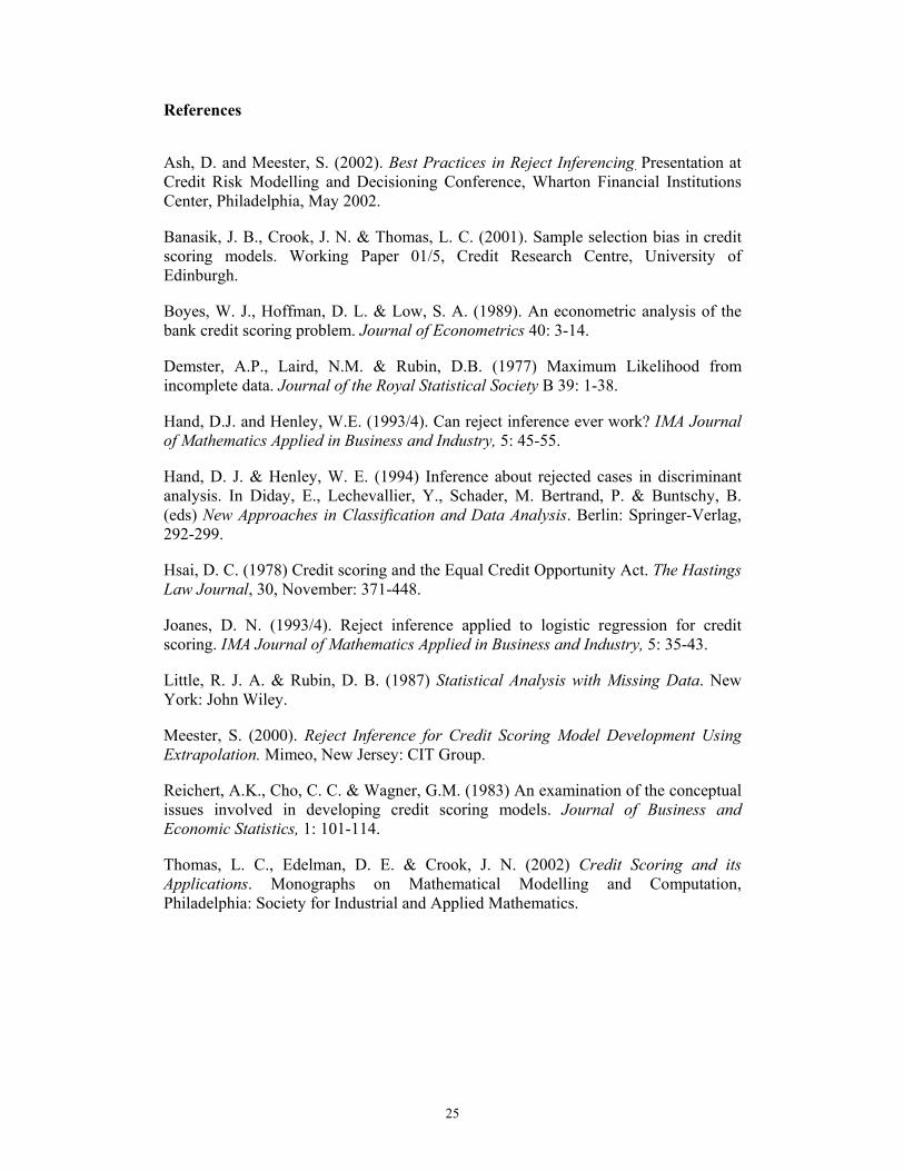
References

Ash, D. and Meester, S. (2002). Best Practices in Reject Inferencing. Presentation at Credit Risk Modelling and Decisioning Conference, Wharton Financial Institutions Center, Philadelphia, May 2002.

Banasik, J. B., Crook, J. N. & Thomas, L. C. (2001). Sample selection bias in credit scoring models. Working Paper 01/5, Credit Research Centre, University of Edinburgh.

Boyes, W. J., Hoffman, D. L. & Low, S. A. (1989). An econometric analysis of the bank credit scoring problem. Journal of Econometrics 40: 3-14.

Demster, A.P., Laird, N.M. & Rubin, D.B. (1977) Maximum Likelihood from incomplete data. Journal of the Royal Statistical Society B 39: 1-38.

Hand, D.J. and Henley, W.E. (1993/4). Can reject inference ever work? IMA Journal of Mathematics Applied in Business and Industry, 5: 45-55.

Hand, D. J. & Henley, W. E. (1994) Inference about rejected cases in discriminant analysis. In Diday, E., Lechevallier, Y., Schader, M. Bertrand, P. & Buntschy, B. (eds) New Approaches in Classification and Data Analysis. Berlin: Springer-Verlag, 292-299.

Hsai, D. C. (1978) Credit scoring and the Equal Credit Opportunity Act. The Hastings Law Journal, 30, November: 371-448.

Joanes, D. N. (1993/4). Reject inference applied to logistic regression for credit scoring. IMA Journal of Mathematics Applied in Business and Industry, 5: 35-43.

Little, R. J. A. & Rubin, D. B. (1987) Statistical Analysis with Missing Data. New York: John Wiley.

Meester, S. (2000). Reject Inference for Credit Scoring Model Development Using Extrapolation. Mimeo, New Jersey: CIT Group.

Reichert, A.K., Cho, C. C. & Wagner, G.M. (1983) An examination of the conceptual issues involved in developing credit scoring models. Journal of Business and Economic Statistics, 1: 101-114.

Thomas, L. C., Edelman, D. E. & Crook, J. N. (2002) Credit Scoring and its Applications. Monographs on Mathematical Modelling and Computation, Philadelphia: Society for Industrial and Applied Mathematics.

Does Reject Inference Really Improve the Performance of

Documents

Transcript of Does Reject Inference Really Improve the Performance of