Does diversification destroy value? Evidence from industry...
42
Does diversification destroy value? Evidence from industry shocks Owen A. Lamont Graduate School of Business, University of Chicago and NBER Christopher Polk Kellogg Graduate School of Management, Northwestern University First draft: December 15, 1999 This draft: July 11, 2000 JEL Classification: G34 Key words: diversified firms, internal capital markets We thank Raghuram Rajan, Henri Servaes, and Luigi Zingales and seminar participants at Chicago for helpful comments. Lamont was supported by the Center for Research in Securities Prices, the University of Chicago Graduate School of Business, the National Science Foundation, and the Alfred P. Foundation. Corresponding author: Owen Lamont, Graduate School of Business, University of Chicago, 1101 E. 58th St., Chicago IL 60637, phone (773) 702-6414, fax (773) 702-0458. [email protected] Revisions available at: http://gsbwww.uchicago.edu/fac/owen.lamont
Transcript of Does diversification destroy value? Evidence from industry...

Does diversification destroy value? Evidence from industry shocks
Owen A. LamontGraduate School of Business, University of Chicago and NBER
Christopher PolkKellogg Graduate School of Management, Northwestern University
First draft: December 15, 1999This draft: July 11, 2000
JEL Classification: G34Key words: diversified firms, internal capital markets
We thank Raghuram Rajan, Henri Servaes, and Luigi Zingales and seminar participants atChicago for helpful comments. Lamont was supported by the Center for Research in SecuritiesPrices, the University of Chicago Graduate School of Business, the National Science Foundation,and the Alfred P. Foundation.
Corresponding author: Owen Lamont, Graduate School of Business, University of Chicago, 1101E. 58th St., Chicago IL 60637, phone (773) 702-6414, fax (773) [email protected]
Revisions available at: http://gsbwww.uchicago.edu/fac/owen.lamont

Does diversification destroy value? Evidence from industry shocks
Abstract
Does corporate diversification reduce shareholder value? Since firms endogenously choose to
diversify, exogenous variation in diversification is necessary in order to draw inferences about
the causal effect. We examine changes in the within-firm dispersion of industry investment, or
“diversity.” We find that exogenous changes in diversity, due to changes in industry investment,
are negatively related to firm value. Thus diversification destroys value, consistent with the
inefficient internal capital markets hypothesis. This finding is not caused by measurement error.
We also find that exogenous changes in industry cash flow diversity are negative related to firm
value.
Does diversification destroy value? - Page 1
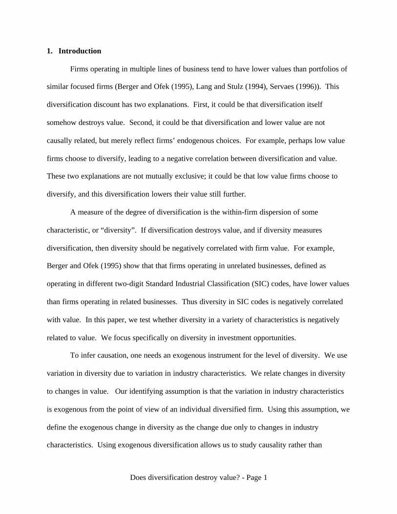
1. Introduction
Firms operating in multiple lines of business tend to have lower values than portfolios of
similar focused firms (Berger and Ofek (1995), Lang and Stulz (1994), Servaes (1996)). This
diversification discount has two explanations. First, it could be that diversification itself
somehow destroys value. Second, it could be that diversification and lower value are not
causally related, but merely reflect firms’ endogenous choices. For example, perhaps low value
firms choose to diversify, leading to a negative correlation between diversification and value.
These two explanations are not mutually exclusive; it could be that low value firms choose to
diversify, and this diversification lowers their value still further.
A measure of the degree of diversification is the within-firm dispersion of some
characteristic, or “diversity”. If diversification destroys value, and if diversity measures
diversification, then diversity should be negatively correlated with firm value. For example,
Berger and Ofek (1995) show that that firms operating in unrelated businesses, defined as
operating in different two-digit Standard Industrial Classification (SIC) codes, have lower values
than firms operating in related businesses. Thus diversity in SIC codes is negatively correlated
with value. In this paper, we test whether diversity in a variety of characteristics is negatively
related to value. We focus specifically on diversity in investment opportunities.
To infer causation, one needs an exogenous instrument for the level of diversity. We use
variation in diversity due to variation in industry characteristics. We relate changes in diversity
to changes in value. Our identifying assumption is that the variation in industry characteristics
is exogenous from the point of view of an individual diversified firm. Using this assumption, we
define the exogenous change in diversity as the change due only to changes in industry
characteristics. Using exogenous diversification allows us to study causality rather than

Does diversification destroy value? - Page 2
correlation.
One specific explanation for the diversification discount is the inefficient internal capital
markets hypothesis: diversified firms invest inefficiently, spending too little on their good
segments and too much on their bad segments. Berger and Ofek (1995) find that diversified
firms overinvest in segments with poor investment opportunities, and that this overinvestment is
related to lower firm value. This explanation implies that diversity in investment opportunities
destroys value, since diversity creates a situation in which the firm can inefficiently transfer
funds from good segments to bad segments.
A variety of other evidence supports this cross-subsidization hypothesis. Lamont (1997)
finds that when oil prices fall, oil firms lower their investment in non-oil segments. Shin and
Stulz (1998) find that more generally, investment of one part of the firm is affected by cash flow
in another part of the firm. Scharfstein (1998) tests predictions from Scharfstein and Stein
(2000), and finds that diversified firms invest too much in low Q segments and too little in high
Q segments, consistent with intra-firm "socialism". Rajan, Servaes, and Zingales (2000) present
a model where resources flow to inefficient divisions, depending both on segments' size and on
their investment opportunities. They examine segment investment, segment size, and industry Q,
and find evidence consistent with their theory. They also find that firm value is negatively
related to diversity in investment opportunities. We test this last finding of Rajan, Servaes, and
Zingales (2000), and in particular we test for a causal connection between diversity and value.
In addition to endogeneity, measurement error is a major issue when drawing inferences
about the effect of diversification. Chevalier (1999) and Whited (1999) study the effects of
measurement error, and argue that it explains some of the evidence on the inefficient internal
capital markets hypothesis. Measurement error is a particular concern when studying the

Does diversification destroy value? - Page 3
relationship between diversity and excess value, because both the diversity measure and the
excess value measure are calculated using the same underlying segment and industry data.
For example, diversity in investment opportunities can be measured using the diversity of
industry Q's for each segment. However, the same industry Q's are also used to calculate the
dependent variable, excess value. Thus measurement error potentially produces a mechanical
correlation between the dependent and independent variable, leading to spurious inferences. For
this reason, we measure diversity in investment opportunities using diversity in industry
investment, not industry Q's. Industry investment should be correlated with industry investment
opportunities, but less correlated with measurement error in industry Q. Since the variable used
to generate diversity is different than the variable used to calculate excess value, hardwiring is
less of a problem. We quantify the potential effect of measurement error, and find it to be small
for our baseline specification.
The following example illustrates our empirical strategy of using industry shocks to
identify the causal effect of diversity. Consider a diversified firm with two divisions of equal
size, an aircraft division and an electronics division. Suppose the aircraft industry has much
lower investment opportunities than the electronics industry, so that the firm has a high diversity
in investment opportunities. We observe this diversity in investment opportunities by observing
that focused firms in the aircraft industry have lower investment than focused firms in the
electronics industry. According to the inefficient internal capital markets hypothesis, the
diversified firm will spend too much on its aircraft division and too little on its electronics
division, and this misallocation will cause the firm to have low value. Perhaps the firm follows a
"fair" rule of splitting the capital expenditures evenly between the two divisions. Now suppose
that, due to changing industry conditions, investment opportunities in the aircraft industry

Does diversification destroy value? - Page 4
improve. This change will decrease the firm's diversity of investment opportunities, and as a
result the "fair" allocation is less harmful. Thus an exogenous decrease in diversity, caused by
industry shocks, leads to a decrease in misallocation and an increase in relative firm value.
To preview the results, we find that exogenous changes in investment diversity are
negatively related to changes in excess value. Thus the observed diversification discount is not
just a consequence of selection biases and endogenous choices by firms. Further, we show that
measurement error is a very unlikely explanation for the negative effect of exogenous diversity.
The contribution of this paper is to show the causal effect of diversification: diversification
destroys value. This finding supports the inefficient internal capital markets hypothesis. We
also find a negative relation between endogenous diversification and value. This finding is more
ambiguous, but is consistent with the self-selection hypothesis that firms diversify in response to
poor performance.
We also examine changes in diversity in industry leverage, sales growth, and cash flow.
Changes in diversity in these other variables do not subsume exogenous changes in investment
diversity, so in this sense the inefficient internal capital markets hypothesis survives. We find
evidence that cash flow diversity, but not leverage or sales growth diversity, destroys value.
Investment diversity does not subsume cash flow diversity.
This paper is organized as follows. Section 2 describes previous research. Section 3
describes the sample and the construction of variables measuring exogenous and endogenous
changes in diversity. Section 4 presents results for diversity in investment opportunities
measured using industry investment. Section 5 explores diversity in other industry
characteristics, including capital structure, profitability, and sales growth. Section 6 presents
conclusions.

Does diversification destroy value? - Page 5
2. Previous research
In addition to the inefficient internal capital markets hypothesis, there are many general
ways in which unrelatedness might reduce value. It may be that managers have limited expertise
and cannot effectively manage diverse businesses, or that unrelated segments have conflicting
operational styles or corporate cultures. This broader explanation also predicts that diversity of
characteristics is negatively correlated with value.
Other theories predict a positive relation between diversity and value. In Lewellen
(1971) diversity of cash flow variation is good if it allows greater tax benefits of leverage by
reducing the volatility of cash flows and the probability of financial distress. Hadlock, Ryngaert,
and Thomas (1999) argue that diversity might be good if managers’ private information at the
segment level washes out at the firm level, reducing information asymmetry. Another argument
is that diversity in investment opportunities is good when internal capital markets function better
than external markets, since it maximizes the scope of the internal market. Hubbard and Palia
(1999) find evidence, using acquisitions in the 1960's, that gains are greatest when a financially
unconstrained buyer acquires a constrained target. Thus diversity in financial constraints is
good. For more on the possible benefits of diversity, see Fulghieri and Hodrick (1997), Stein
(1997) and Wulf (1998).
Value destruction or creation can occur in two ways. The value of any asset is the sum of
discounted future cash flows, so that value can change either due to changes in cash flows or
changes in discount rates. Lamont and Polk (1999) show that a substantial fraction of the cross-
sectional variance of diversification discounts is due to variation in expected returns; firms with
high expected returns have low values, and firms with low expected returns have high values.
Most existing empirical work has focused on potential cash flow effects of diversification (for

Does diversification destroy value? - Page 6
example, studies of profits or productivity in diversified firms). One could also imagine discount
rate versions of existing explanations. For example, perhaps inefficient cross-subsidization
involves taking excessively risky projects with high discount rates. We do not attempt to
discriminate between these two sources of value destruction in this paper.
A variety of papers examine endogenous changes in diversity, in which firms choose to
diversify (usually through an acquisition) or focus (usually through spinoffs or divestitures).
Several studies test whether endogenous diversifying behavior leads to a negative correlation of
diversity and value by studying whether firms have low value and poor performance before
diversifying (Lang and Stulz (1994), Hyland (1999), Campa and Kedia (1999), Graham,
Lemmon, and Wolf (1999)).
A frequent finding is that refocusing raises firm value, as in Comment and Jarrell (1995)
and John and Ofek (1995). Daley, Mehrotra , and Sivakumar (1997) find that spun-off segments
experience improved performance, especially if they are unrelated (see also Kaplan and
Weisbach, (1992)). Gertner, Powers, and Scharfstein (1999) find that the investment of spun-off
segments changes in a way consistent with the inefficient internal capital markets hypothesis.
Berger and Ofek (1996, 1999) find that takeovers, leveraged buy-outs, shareholder pressure,
managerial turnover, and other largely external sources are the cause of much refocusing. These
findings are consistent with the idea that diversification destroys value, and that the market for
corporate control helps eliminate value-destroying diversification (for related work, see also
Schlingemann, Stulz, and Walkling, 1999 and Peyer and Shivdasani, 2000).
If the decision to diversify reflects value-destroying managerial waste, one might expect
endogenous increases in diversity to decrease value. Morck, Shleifer, and Vishny (1990) and
Maquiera, Meggison, and Nail (1998) find that acquiring firm stockholders lose value in

Does diversification destroy value? - Page 7
diversifying acquisitions. Schoar (1999) finds that firms that acquire plants in unrelated
industries experience a subsequent decrease in total firm productivity. If in contrast, firms
optimally choose to diversify (as in Maksimovic and Phillips (1999) and Fluck and Lynch
(1999)), one might expect all endogenous changes in diversification to have a positive effect,
reflecting firms moving closer to the optimum. Of course, since endogenous actions are taken in
response to events that the econometrician cannot observe, the observed correlation between
endogenous diversification and value that we measure can never be conclusive about whether
firms are behaving optimally.
3. Sample and Variable Construction
3.1. Data
Our sample consists of firms reporting segment data in the Compustat Current and
Research database, 1979-1997. The data sources and variables are described more fully in the
appendix. Following Berger and Ofek (1995), we discard firm-years with segments in the
financial services industry, total firm sales of less than $20 million, or discrepancies in segment
and firm data. We also require firms to have information on firm-level equity, debt, investment,
capital stock, and sales growth. The only segment level data we use are sales, assets, and SIC
codes for each individual segment.
Our measure of excess value is based on market-book ratios. Q is the ratio of the market
value of the firm (the market value of common stock plus the book value of total assets minus
book equity minus deferred taxes) divided by the total book assets of the firm.1 For each
segment of a diversified firm, we find a group of matching focused firms with the same two-digit
SIC code. We then calculate the median for each segment’s industry, QIND. We drop every
diversified firm that does not have at least five matching focused firms for each of its segments.

Does diversification destroy value? - Page 8
We then form Q , the imputed value ratio, for the entire diversified firm as the weighted average
of the industry QIND's:
{ }( )∑∑==
==n
jNj
n
jjINDj j
QQQmedianwQwQ1
211
,...,, (1)
where wj is the fraction of the firm's assets in segment j, Qi is market-book for focused
company i, segment j's industry has Nj focused firms, and the firm has n segments. We measure
excess value by taking the log ratio, q- q = ln(Q/ Q ), as in Berger and Ofek (1995). Lower case
letters indicate natural logs.
Our identification strategy requires using annual changes in variables. The change in
excess value, ∆q-∆ q , is the difference between excess value for a given diversified firm
between year t-1 and year t. For the purposes of defining our sample, we classify a firm as
diversified in year t if it has multiple segments in year t-1. This classification allows us to
examine exogenous and endogenous changes in diversity for firms that decrease their number of
segments between year t-1 and year t. We classify a firm as focused if it has one segment in both
year t and year t-1. We discard firms that have one segment in year t-1 and multiple segments in
year t, because such firms have no exogenous change in diversity between year t-1 and year t.
3.2. Endogenous and exogenous changes in diversity
Our measure of diversity of some characteristic is the within-firm standard deviation of
the segment characteristics in a given year. All the characteristics we examine are industry
benchmarks that come from the matching sample of focused firms. Our main focus is on
dispersion in investment opportunities within the firm, measured by dispersion in industry
investment. For a given segment and year, we measure industry investment, IIND, as that year's
median investment to capital ratio among focused firms in the segment’s two-digit industry. For

Does diversification destroy value? - Page 9
each focused firm, investment to capital is year t capital expenditures divided by year t-1 net
capital stock (book value). For each diversified firm, we measure diversity in year t as σ t, the
standard deviation of IIND for the different segments. The change in diversity is ∆σt. Neither
sales nor assets at the segment level affect this definition of diversity.
Changes in diversity reflect both changes in the structure of the individual firm and
changes in industry characteristics. We call changes due to industry characteristics alone
“exogenous changes” (reflecting actions not taken by the individual firm) and changes due to
reported corporate structure as “endogenous changes”. Let structuret be firm structure in year t,
defined as the number and industry classification of segments. Let benchmarkt be the set of
industry characteristic values as of year t. Then the change in diversity is:
∆σ t ≡ σ t - σ t-1 (2)
= σ(structuret, benchmarkt) - σ( structuret-1, benchmarkt-1)
= [σ(structuret, benchmarkt) - σ(structuret-1, benchmarkt)]
+ [σ( structuret-1, benchmarkt)- σ( structuret-1, benchmarkt-1) ]
≡ ∆σN + ∆σX
The exogenous change in diversity, ∆σX, is the change in diversity between t-1 and t that
would have taken place if the firm had not changed its structure between t-1 and t. Since this
change is caused only by changes in industry characteristics (which we assume are not affected
by actions taken by the firm), these changes are exogenous to the firm.
The endogenous change in diversity, ∆σN, is the change in diversity that takes place due
to changes in firm structure between t-1 and t. In order for ∆σN to be nonzero, a firm must either
add a new segment, delete an existing segment, or change the activities of an existing segment
such that Compustat assigns it a new SIC code. An endogenous change in diversity can take

Does diversification destroy value? - Page 10
place either because the firm changes its actual structure, or merely because the firm changes its
reported structure. Either way, this change in reported structure reflects endogenous decisions
by the firm.
The observed change in corporate structure reflected in ∆σN is probably a very noisy
indicator of economic changes in structure. Segment data only loosely corresponds to major
events such as acquisitions and divestitures. Hyland (1999) examines a sample of 227 firms that
increase the number of segments, 1978-1992. He finds that 150 (66 percent) are due to
acquisitions, 23 (10 percent) are due to internal growth, and 54 (24 percent) are due to reporting
changes only (Graham, Lemmon, and Wolf (1999) find similar results in a 1980-1995 sample).
Berger and Ofek (1999) examine a sample of 295 firms decreasing their number of segments,
1984-1993, and find that 107 (36 percent) cases represent true refocusing as opposed to reporting
changes.
Table 1 shows an example from our dataset. In 1996, Northrop Grumman had two
segments, an aircraft segment with industry investment of 17.6 percent, and an electronics
segment with industry investment of 33.2 percent. Since industry median investment to capital
ratios (reflecting investment by focused firms) were quite different for aircraft and electronics in
1996, by our measure Northrop Grumman was a fairly diverse firm. It also had a sizable
discount of 29 percent, as its Q was below its imputed value. In 1997, Northrop Grumman
changed its structure to include a third segment, Information Technology and Services. This
change in segment reporting reflects both an acquisition in 1997 and a reclassification of existing
assets (largely from the electronics division) into the new segment.
Northrop Grumman’s diversity measure changed in two ways between 1996 and 1997.
First, an increase in aircraft industry investment caused an exogenous decrease in diversity as

Does diversification destroy value? - Page 11
aircraft and electronics investment became more similar (Table 1 also shows that aircraft
industry Q also rose substantially). Had the firm not added a new segment, the changes in
aircraft and electronics alone would have resulted in a decrease in diversity, from 11 percent to
7.2 percent. Thus the exogenous change in diversity is -3.8 percent. Second, the addition of a
third segment with very high industry investment increased diversity, to a total of 19.6 percent.
Thus the endogenous change in diversity is the difference between 7.2 percent and 19.6 percent,
or 12.4 percent.
Table 2 shows summary statistics and cross-correlations for the sample of diversified
firms. The sample contains 11,974 annual observations for 1,987 different diversified firms in
the 18 year period of 1980-1997. The average number of segments per firm is 2.7. The number
of firms per year declines over time, from a high of 872 in 1981 to a low of 482 in 1997.
Average and median excess values are negative at -2.8 and -6.1 percent.2 Since the standard
deviation of exogenous diversity change is 0.040 and the standard deviation of total diversity
change is 0.045, most (80 percent) of the variation in diversity change is due to exogenous
industry shocks.
4. Diversity in investment
Table 3 shows basic results for regressions of changes in excess value on changes in
diversity in industry investment. The regression is simple pooled OLS; the standard errors have
been adjusted for correlation of the residuals within years, and for heteroskedasticity. 3 The first
column shows that the coefficient on the change in diversity is negative and significant. The
coefficient implies that a one standard deviation increase in diversity lowers excess value by 1.1
percent.
One can use the coefficient on ∆σ to calculate the potential contribution of diversity in

Does diversification destroy value? - Page 12
explaining the average level of the diversification discount. Mechanically, a focused firm has a
σ of zero. Since the mean of σ is 0.049, the average level of diversity explains an average
discount of -0.25*0.049 or 1.2 percent. Since the average discount in this sample is 2.8 percent,
more than 40 percent of the level of the average discount can be explained with investment
diversity alone.
Column (2) shows the results using the exogenous change in diversity. Exogenous
changes in diversity have a negative and significant effect on excess value. This finding is the
major result of this paper: diversification is negatively correlated with value not just due to
selection biases and endogenous choices by firms, but also because higher levels of
diversification somehow cause value destruction.
Column (3) shows that both exogenous and endogenous changes in diversity are
negatively related to changes in excess value. Thus as often hypothesized, an important reason
for the negative correlation of diversification and value is endogenous diversifying behavior by
firms. Unlike the coefficient on exogenous diversity, however, one cannot interpret the
coefficient on endogenous diversity as evidence that diversification destroys value. The
coefficient could reflect several possibilities: value-destroying diversification, value-creating
diversification in response to some unobserved negative shock to the firm, or a tendency of
diversified firms to acquire low value businesses (Graham, Lemmon, and Wolf, (1999)) or divest
high value businesses.
Column (4) adds to the regressions the year t-1 level of excess value, the year t-1 level of
investment diversity, and year and firm fixed effects. The year and firm fixed effects are
separate dummy variables for each of the 18 years and each of the 1987 firms. Including the
lagged levels of excess value and diversity is meant to capture predictable mean reversion in

Does diversification destroy value? - Page 13
these variables. The negative coefficient on lagged excess value reflects the fact that excess
value tends to move towards its mean. Economically, this mean reversion can occur because
firms with high excess values invest more (so that their book value goes up and the ratio of
market to book falls), or because they tend to have low subsequent returns (so their market value
goes down), as in Lamont and Polk (1999).
Including the lagged level of diversity helps to control for predictable movements in
diversity. As seen in Table 2, exogenous changes in diversity are quite predictable using the
lagged level of diversity, since the correlation between the two variables is -0.40. Expected
changes in diversity (due to expected changes in industry conditions) should already be reflected
in market values as of year t-1. Since we are interested in examining the effects of industry
shocks on value, we want to purge changes in diversity of their expected component. Putting the
lagged level of diversity into the regression is a simple way of accomplishing this goal.
These additional control variables do not change the basic result that both exogenous and
endogenous changes in diversity are negatively related to firm value. The coefficient on
exogenous changes rises somewhat, while the coefficient on endogenous diversity is little
changed. We use column (4) as our baseline regression.
4.1. Effects of measurement error
Measurement error is an issue in Table 3 since both the dependent variable and the
independent variable are constructed using the same segment information and industry
characteristics. If the segment information (such as SIC codes) or the characteristics are
observed with error, this measurement error can lead to faulty inferences. In the case of industry
characteristics, the most relevant source of measurement error is probably inappropriate
matching of focused firms with diversified firm segments (see Chevalier (1999)). If focused

Does diversification destroy value? - Page 14
firms are fundamentally different from diversified firms, or if there is some noise in the process
of matching focused firms to diversified firms, then industry characteristics will be noisy
measures of firm value and of segment characteristics.
Other sources of measurement error include Compustat coding errors, a major issue in the
segment database. Lamont (1997) examined segment data for 26 firms between 1985 and 1987
and found coding errors in four (15 percent). Hyland (1999) found examined segment data for
243 firms between 1978 to 1992, and found coding errors in 29 (12 percent), of which 16
involved backfilling of segment data.
The same measurement error appearing in both the dependent and independent variables
can lead to spurious results. In interpreting the regression coefficients in columns (1) and (2) of
Table 3, the following simple framework is helpful. Suppose the true relationship is
∆q-∆ *q = α+β∆d* +ε (3)
where *q is the true log imputed value ratio for the firm and d* is the true diversity measure. We
observe noisy measures of the true variables:
∆ q =∆ *q +u (4)
∆d=∆d*+v (5)
Since both ∆ q and ∆d are constructed using the same underlying variables, in general both
cov(∆ *q ,∆d*) and cov(v,u) will be non-zero. If one regresses is ∆q-∆ q on ∆d, the estimated
coefficient (assuming that the measurement errors, u and v, are uncorrelated with the disturbance
term ε) is
b)var()var(
),cov()var(*
*
vduvd
+∆−∆
=β
)var()var(),cov(
)var()var()var(
**
*
vduv
vdd
+∆−
+∆∆
= β (6)

Does diversification destroy value? - Page 15
Measurement error induces a biased coefficient in two ways. First, the familiar
attenuation effect ()var()var(
)var(*
*
vd
d
+∆
∆) moves the coefficient towards zero. Second, the
covariance term ()var()var(
),cov(* vd
uv
+∆− ) causes b to be biased either positively or negatively.
We call this second term “covariance bias,” and consider it separately from attenuation.
While we cannot directly observe the covariance bias, we can observe
c=)var()var(
),cov(),cov(*
**
vd
dquv
+∆
∆∆+, which is the coefficient in a regression of ∆ q on ∆d. With a
further assumption about the measurement error, we can bound the covariance bias. Let ρ be the
fraction of cov(∆ q , ∆d) that is due to measurement error, ρ = ),cov(
),cov(dq
uv∆∆
. The covariance
bias is then -ρc. A natural extreme value of ρ is one, which corresponds to a scenario in which
the matching procedure is completely useless and measurement error is so large that either the
diversity measure or q (or both) are complete noise. Although any value of ρ is possible, values
between zero (corresponding to no measurement error) and one (corresponding to huge
measurement error) seem most reasonable. We leave it to the readers to choose ρ as they see fit.
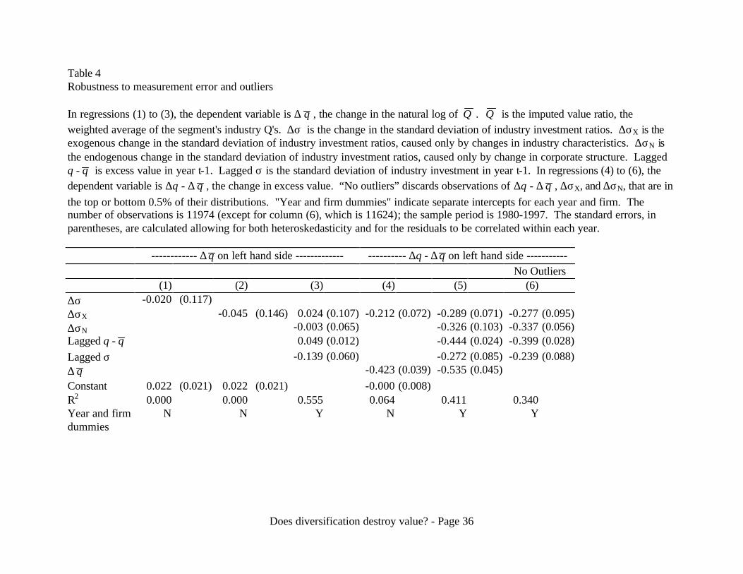
Columns (1) and (2) in Table 4 show estimates of the coefficient c. Consider the
regression in column (2) of Table 3, which shows a coefficient of -0.193 for exogenous changes
in diversity. Column (2) of Table 4 shows that for this regression, c is -0.045. Thus if ρ is
between zero and one, the true coefficient actually has a higher magnitude than the estimated
coefficient, as both attenuation bias and covariance bias move the estimate towards zero. Thus
measurement error cannot explain the negative and significant coefficient in column (2) of Table
3.

Does diversification destroy value? - Page 16
Column (3) of Table 4 shows the multiple regression version with change in log imputed
value as the dependent variable and our baseline variables on the right hand side. The coefficient
for exogenous diversification is now positive but low at 0.024. This positive coefficient with
∆ q as the dependent variable obviously tends to produce a negative coefficient when ∆q - ∆ q is
the dependent variable. Compared to the coefficient of -0.302 in column (4) of Table 3,
however, the coefficient of 0.024 seems basically irrelevant.
Columns (4) and (5) of Table 4 show the effect of adding ∆ q to the right-hand side of the
regressions. First, column (4) adds change in imputed value to the two-variable regression.
Using the measurement error framework, in this regression the covariance bias is positive if ρ is
greater than 0.42.4 Despite a potentially positive bias when measurement error is extreme,
exogenous changes in diversity still have a negative and significant effect. Including ∆ q in the
baseline specification, in column (5), slightly lowers the coefficient on exogenous changes in
diversity, but the coefficient is still negative and significant.
The last column of Table 4 discards extreme observations, defined as any observation
which is in the top 0.5% or bottom 0.5% of the distribution of ∆q -∆ q , ∆σN, and ∆σX. The
coefficient on the exogenous changes in diversity is slightly lower than the baseline results, but is
still negative and significant.
In summary, our results are very unlikely to be driven by measurement error. As we will
see later, however, measurement error can be an important concern when using other measures
of diversity in investment opportunities.
4.2. Alternative specifications
Table 5 explores the stability of our main results. Since our main interest is the causal
role of diversity, we focus on the coefficient on exogenous diversity change. Column (1) shows

Does diversification destroy value? - Page 17
the results of discarding diversified firms that have any segments in nonmanufacturing
industries. One might expect measurement error in diversity to be lower in this regression, since
investment to capital ratios are less well-behaved in nonmanufacturing industries such as
services, mining, and agriculture. Column (1), which has a sample size of about half the baseline
sample, shows the coefficient on exogenous change in diversity rises and remains significant.
Column (2) shows a version of the baseline regression replacing Q everywhere with M,
the ratio of the market value to the total sales of the firm. The coefficient on exogenous diversity
is again stronger compared to the baseline results. The coefficient on endogenous diversity is
much higher but is estimated imprecisely. Column (3) measures diversity using the coefficient
of variation of industry investment (the ratio of standard deviation to mean), rather than the
standard deviation of industry investment. Again, the exogenous change in diversity has a
significant negative effect (the coefficient is different from the baseline regression because the
units of the diversity change variable are different). Column (4) shows the effects of calculating
excess value using differences in Q rather than log differences, and column (5) uses Fama-
Macbeth estimation; the coefficients on the exogenous change in diversity remain negative and
significant.
In summary, our results are robust to alternate specifications, and are especially strong
for manufacturing firms. This robustness to alternate specifications again suggests that
measurement error or misspecification is not the driving factor.
4.3. Alternate measures of diversity in investment
Here we explore two alternate measures of investment diversity that incorporate
information about the relative size of the various segments. The first measure we examine is
diversity in resource-weighted investment. Rajan, Servaes, and Zingales (2000) present a theory

Does diversification destroy value? - Page 18
in which investment allocation is determined by both the diversity in segment resources and in
segment investment opportunities. They use a measure involving the standard deviation of
investment opportunities multiplied by relative segment size (we examine their specific measure
in the next section).
Our analog is the standard deviation of weighted investment, σ1:
2
1 1
11
11 ∑ ∑
= =
−
−=
n
j
n
iiINDijINDj Iw
nIw
nσ (7)
where again wj is the fraction of the firm's assets in segment j, IIND j is industry investment for
segment j, and the firm has n segments. σ1 is diversity in asset-weighted investment. According
to σ1, a firm can have high diversity even if industry investment is the same for each segment, as
long as it has segments of different size.
Our second alternate measure of investment diversity takes the opposite approach with
segment size. The weighted standard deviation is σ2:
2
1 112 ∑ ∑
= =
−
−=
n
j
n
iiINDijINDj IwIw
nn
σ (8)
In calculating diversity, σ2 gives more weight to bigger segments. Consider a firm with 99% of
its assets in one segment and 1% of its assets in another segment. Ceteris paribus, while σ1
would view this firm as extremely diverse, σ2 would view this firm as not at all diverse and
almost the same as a focused firm.
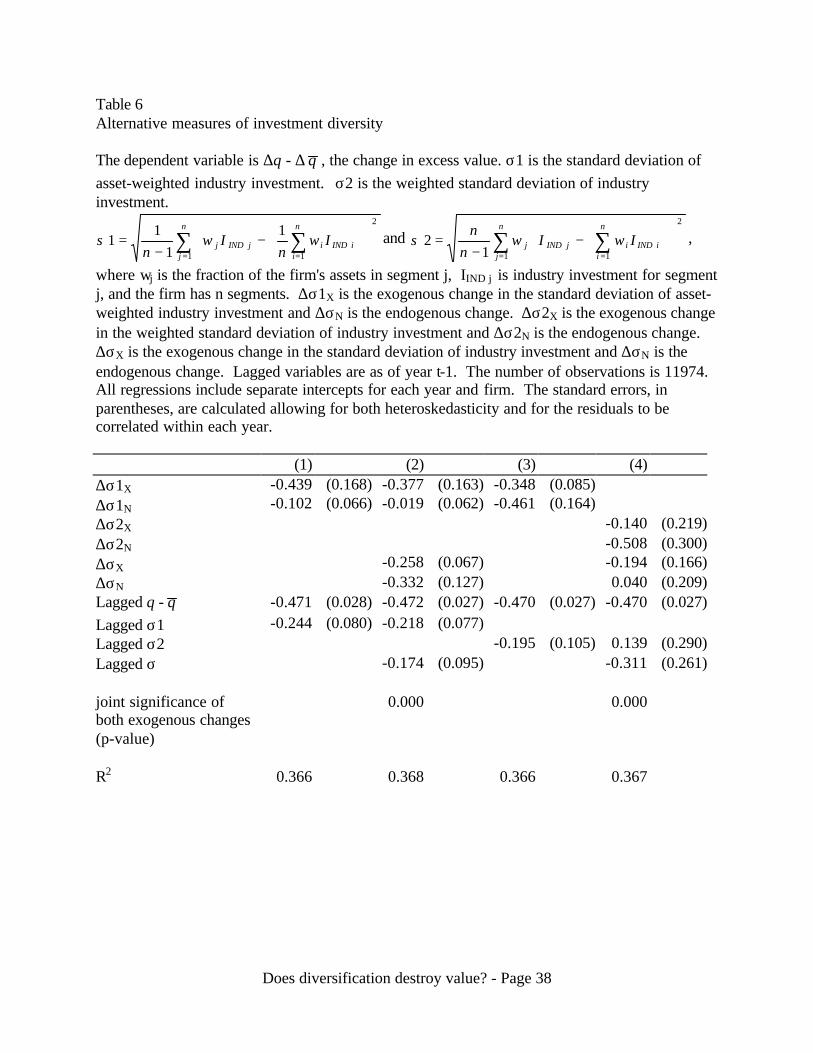
Table 6 shows results for the effect of diversity on excess value, again decomposing the
change in diversity into an exogenous component reflecting changes in industry investment and
an endogenous component reflecting changes in structure (which now include changes in
segment assets). We show the diversity measures by themselves, and then in conjunction with

Does diversification destroy value? - Page 19
our baseline diversity measure. As before, we include the lagged level of the particular diversity
measure.
Column (1) shows the regression using σ1, diversity in asset-weighted investment. As
with the baseline specification, exogenous changes in diversity have a negative and significant
effect on excess value. Column (2) adds changes in baseline diversity. The coefficient on ∆σX is
slightly lower than the coefficient in the baseline specification, and the coefficient on ∆σ1X falls
somewhat. Both exogenous changes are individually significant. Measurement error does not
appear to be a problem in column (2), as the regression (not shown) of ∆ q on column (2)'s right-
hand side variables results in a coefficient of 0.14 on ∆σ1X and -0.01 on ∆σX. Thus there is
evidence that exogenous changes in asset-weighted diversity (in addition to unweighted
diversity) destroy firm value. We interpret this surprising result as a victory for the resource-
weighted approach advocated by Rajan, Servaes, and Zingales (2000).
Column (3) shows the results using σ2, the weighted standard deviation of investment.
The coefficients are similar to the baseline specification. Column (4) shows the effect of adding
σ. It turns out that ∆σX and ∆σ2X have a correlation of 0.95, so that multicollinearity plagues
column (4). Although neither ∆σX nor ∆σ2X are individually significant, they are strongly
significant jointly. Thus we conclude from columns (3) and (4) that it is impossible to tell
whether ∆σX and ∆σ2X have separate effects on value, and that it does not much matter whether
one uses the simple standard deviation or the weighted standard deviation in measuring
investment diversity.
5. Diversity of different characteristics
5.1. Diversity in asset-weighted industry Q
Table 7 examines the diversity measure of Rajan, Servaes, and Zingales (2000), which

Does diversification destroy value? - Page 20
we call RSZ. RSZ is the diversity in asset-weighted Q, and is defined as:
( )∑
∑ ∑−
−
==
= =
jjIND
n
j
n
iiINDijINDj
EW
jINDj
Qn
n
Qwn
Qw
Q
QwstdevRSZ
11
12
1 1
(9)
EWQ is equal weighted industry Q. As in our measure σ1, the RSZ measure involves diversity in
segment size measured by book assets.
Column (1) of Table 7 reproduces basic results on excess value using a first differenced
version of the specification in Rajan, Servaes, and Zingales (2000). In addition to the measure of
diversity, their specification also includes the log of firm size and the inverse of the equal
weighted Q across the segments. The dependent variable is the first difference in excess value,
measured without logs. The regression is not exactly the same as theirs because Rajan, Servaes,
and Zingales (2000) use levels instead of differences, have a shorter time period, match by three
digit SIC codes instead of two, use a more complex measure of Tobin's Q rather than the market-
book ratio, and Winsorize the variables. Nevertheless, the results are broadly similar, as the
coefficient of -0.116 (with t-statistic of 2.5) on diversity corresponds to the estimate of -0.276
(with t-statistic of 5.7) in Rajan, Servaes, and Zingales (2000).
Column (2) splits the change in RSZ into exogenous and endogenous components, where
as before the endogenous change reflects changes in corporate structure and the exogenous
change reflects changes in industry characteristics. Column (2) shows that the effect of diversity
comes largely through exogenous changes in diversity, as the coefficient on the exogenous
change in RSZ is large and significant. Thus column (2) shows that endogeneity is not a major
concern for the Rajan, Servaes, and Zingales (2000) results.5
The major concern in Table 7 is measurement error, since industry Q's now enter directly

Does diversification destroy value? - Page 21
into the diversity measure as well as the dependent variable. Thus measurement error in industry
Q's has a greater potential to produce spurious results. To gauge the effects of measurement
error, we start by putting the exogenous change in RSZ diversity into a two-variable regression.
Column (3) shows the coefficient is still large and significant at -0.459. Column (4), however,
shows the coefficient c is 0.906 in this setting. Thus with a ρ of 0.51, measurement error can
completely explain the estimated coefficient on exogenous change in RSZ. Of course the value
of ρ is a judgement call that the reader must make. Readers who believe measurement error is
not a problem should set ρ=0; conservative readers who want to avoid false inferences should set
ρ higher.
The full specification used by Rajan, Servaes, and Zingales (2000) includes as a control
variable the inverse of average industry Q for the firm's segments. Column (5) shows that this
control variable does not eliminate the covariance bias. In the analogous multiple regression
with the change in Q as the dependent variable, the coefficient of 1.290 in column (5) is large,
and could easily account for the coefficient of -0.664 in column (2).
Thus Table 7 shows that one must be careful in interpreting the empirical results using
the RSZ measure of diversity, since the results are quite sensitive to assumptions about
measurement error. "Hard-wiring" in the construction of the independent and dependent
variables can lead to spurious results. Rajan, Servaes, and Zingales (2000) present a variety of
evidence that measurement error is not driving their results, although most of their robustness
tests involve other regressions with different dependent and independent variables (since
explaining excess value with diversity is not their main focus). For these other regressions, they
perform simulations, experiment with different control variables, and try alternative ways of
constructing the variables. Based on Table 7, we conclude that the Rajan, Servaes, and Zingales

Does diversification destroy value? - Page 22
(2000) results on the relation between excess value and diversity are not convincing evidence in
favor of their hypothesis, but this conclusion is a matter of opinion.
Despite these measurement error issues, we view our basic result, that diversity lowers
firm value, as supporting the central premise of Rajan, Servaes, and Zingales (2000). And, as
shown in Table 6, there is evidence that resource-weighting, as advocated by Rajan, Servaes, and
Zingales (2000), helps explain this value destruction.
5.2. Diversity in other characteristics
Berger and Ofek's (1995) finding that excess values are lower for firms in unrelated
businesses is consistent with the inefficient internal capital markets hypothesis, but is also
consistent with the general notion that unrelated diversification is value destroying. Unrelated
diversification could be bad due to greater scope for inefficient cross-subsidization, but it could
also be bad for other reasons, such as limited managerial talent. Since different industries have
different levels of investment, diversity in industry investment could be proxying for more
general diversity. Broadly, each year we would expect different industries to be different along
many measurable dimensions, such as profitability, capital structure, and sales growth. The
greater the diversity in these values in a given year, the greater the degree of unrelated
diversification.
Table 8 examines diversity in characteristics other than investment. For each
characteristic, we express diversity as the standard deviation in the industry characteristic. Table
8 examines each characteristic by itself and then in combination with investment diversity.
The first variable is leverage, the ratio of book debt to the sum of book debt and market
equity. Lang, Ofek, and Stulz (1995) show that firm leverage is negatively related to capital
expenditures of noncore segments, suggesting that high leverage prevents segments from taking

Does diversification destroy value? - Page 23
advantage of investment opportunities, and that combining segments with high optimal leverage
and low optimal leverage results in value destruction. Table 8 shows that by itself, endogenous
changes in leverage diversity are negatively related to firm value. There is no evidence that
leverage diversity causes lower values, since the exogenous change in leverage has a near zero
effect. Finally, when adding the leverage diversity variables to our baseline regression, the
coefficient on exogenous changes in investment diversity remains negative and significant.
This pattern is repeated for diversity in sales growth, where sales growth is year t net
sales divided by year t-1 net sales. Without investment diversity, only endogenous sales growth
diversity has a negative and significant coefficient, and with investment diversity, both types of
sales growth diversity are insignificant.
Cash flow diversity, however, does have a strong negative effect. Cash flow is the ratio
of income before extraordinary items to prior year capital stock. Without investment diversity,
both endogenous and exogenous changes in cash flow diversity have negative and significant
coefficients. With investment diversity, the cash flow diversity coefficients are little changed.
Compared to the baseline results, the coefficient on the exogenous change in investment
diversity is somewhat lower at -0.210 instead of –0.302, and the coefficient on endogenous
diversity changes falls dramatically. Exogenous investment diversity changes still have a
significant effect, therefore cash flow diversity does not subsume exogenous investment
diversity.
How should one interpret the results on cash flow diversity and investment diversity?
Berger and Ofek (1995) use the presence of a segment with negative cash flow (where the cash
flow being used is actual segment cash flow, not industry cash flow) as a marker for cross-
subsidization. In this sense, low segment cash flow is similar to low segment investment

Does diversification destroy value? - Page 24
opportunities in that it indicates a potential for draining resources from the good segments to
spend on the bad segments. Thus one interpretation of the negative effect of cash flow diversity
is that it supports the inefficient internal capital markets hypothesis, since cash flow diversity
creates a situation where good segments can subsidize bad segments. When the bad segments
get worse and the good segments get better, the cross-subsidization problem becomes more
severe.
In summary, other measures of diversity do not subsume investment diversity. Cash flow
diversity has an independent exogenous effect, however, which could be consistent with the
inefficient internal capital markets hypothesis, but could also reflect the more general idea that
unrelatedness is bad.
6. Conclusions
Diversification destroys value. Our results show that exogenous increases in the diversity
of a firm's investment opportunities reduce firm relative value. Since we look at exogenous
changes due to industry shocks, our results show that selection biases and endogenous
diversifying behavior are not entirely responsible for the observed diversification discount. We
also study the effect of measurement error, and find that although measurement error can cause
spurious results for some specifications, our specification is relatively immune. These results
support the inefficient internal capital markets hypothesis: diversified firms have low value
because they allocate capital inefficiently across their different parts.
Our analysis has limitations. It does not imply that if one randomly aggregated focused
firms into diversified firms, value would be destroyed. What we show is that exogenous
increases in diversity destroy value, conditional on already being diversified.
We find that when firms endogenously choose to become more diversified, their excess
Does diversification destroy value? - Page 25
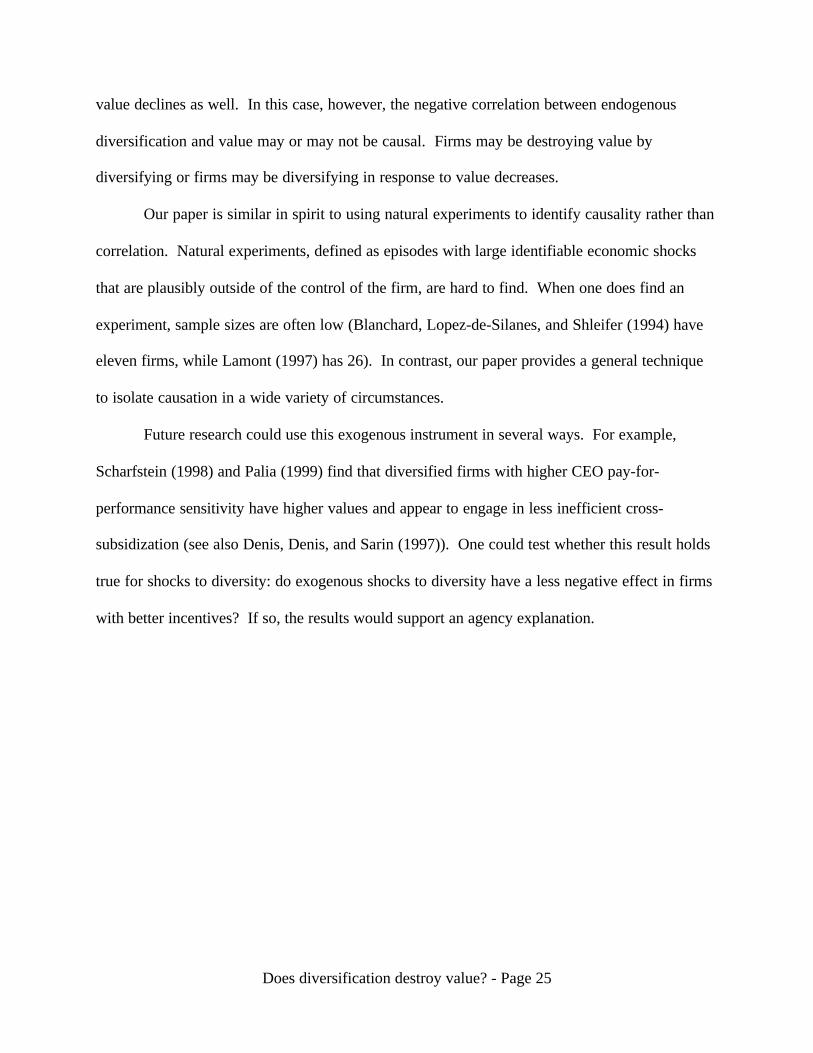
value declines as well. In this case, however, the negative correlation between endogenous
diversification and value may or may not be causal. Firms may be destroying value by
diversifying or firms may be diversifying in response to value decreases.
Our paper is similar in spirit to using natural experiments to identify causality rather than
correlation. Natural experiments, defined as episodes with large identifiable economic shocks
that are plausibly outside of the control of the firm, are hard to find. When one does find an
experiment, sample sizes are often low (Blanchard, Lopez-de-Silanes, and Shleifer (1994) have
eleven firms, while Lamont (1997) has 26). In contrast, our paper provides a general technique
to isolate causation in a wide variety of circumstances.
Future research could use this exogenous instrument in several ways. For example,
Scharfstein (1998) and Palia (1999) find that diversified firms with higher CEO pay-for-
performance sensitivity have higher values and appear to engage in less inefficient cross-
subsidization (see also Denis, Denis, and Sarin (1997)). One could test whether this result holds
true for shocks to diversity: do exogenous shocks to diversity have a less negative effect in firms
with better incentives? If so, the results would support an agency explanation.

Does diversification destroy value? - Page 26
APPENDIX
Data Sources and Definitions
Our data on segments comes from several Current and Research segment files obtained
from Wharton Research Data Services in April 1999. Our firm-level Compustat and Center for
Research in Securities Prices (CRSP) data comes from the University of Chicago’s database in
December 1999. In our calculation of market value, we use CRSP market equity. For firms with
multiple classes of stock, in calculating market equity, we aggregate all separate classes of stock
together into one value-weighted portfolio.
We define Q as {market capitalization (from CRSP) + book assets (data item 6) - book
equity (data item 60) - deferred taxes (data item 74)} / book assets (data item 6). The investment
to capital ratio is capital expenditures (data item 128) divided by prior year net stock of property,
plant, and equipment (data item 8). The market-sales ratio, M, is (total debt + market
capitalization) / net sales (data item 12). Leverage is total debt / (total debt + market
capitalization) where total debt is defined as long-term debt (data item 9) + debt in current
liabilities (data item 34) + redemption value of preferred stock (data item 56). The cash flow is
the sum of income before extraordinary items (data item 18) and depreciation and amortization
(data item 14), divided by prior year net stock of property, plant, and equipment (data item 8).
Screening
We drop firm-years if any of the following conditions hold: it has missing or nonpositive
firm sales or firm assets; missing or nonpositive (for any segment) segment sales or segment
assets; has any segment which Compustat assigns an 1-digit SIC code of 0, 6 (financial), or 9
(largely "NO OPERATIONS"); the sum of segment sales is not within 1 percent of the total sales
of the firm; the firm changes the month of its fiscal year-end such that in December of year t-1
Does diversification destroy value? - Page 27
our latest information is from year t-2. We also drop firms (such as GM) who report multiple
firm totals for the same year (firms which report different Compustat total sales for the same
CRSP permanent company identifier number).

Does diversification destroy value? - Page 28
FOOTNOTES 1 For convenience, we use the letter Q to describe this variable, although it is not precisely the
same as the standard variable called Tobin's Q, which involves more complicated calculations of
replacement value.
2 In interpreting the values it is important to note that the natural logarithm is a concave function.
Since firm-level variables are more volatile than industry-level variables, average log ratios tend
to be negative. For example, mean Q is above mean Q , but mean qq − is negative. Looking at
excess value without logs, the mean of Q - Q is 3.9 percent and the median is -6.8 percent.
3 The robust standard errors allow for clustered sampling (dependence of observations within
each year), following Rogers (1993).
4 Using the measurement error framework, the coefficient on exogenous change in diversity is
[ ])var(
),cov()var()var(
)var(),cov(
),cov(),cov()var(
2*
***
qdq
vd
qdq
qqdqd
∆∆∆
−+∆
∆∆∆
∆∆−∆∆+∆β. The bottom of this fraction is
positive. The sign of the covariance bias depends on the sign of
)var(),cov(
),cov()1)(,cov(q
dqqqdq
∆∆∆
∆∆−−∆∆ ρ . Plugging in numbers, the sign of the bias is
negative as long as ρ is less than 0.42.
5 In the working paper version, Rajan, Servaes, and Zingales (1998) perform a robustness test
that is somewhat similar to our exogenous/endogenous distinction. They show that their results
survive after dropping firms for which individual segments experience large changes in asset
value. They also control for the number of segments. However, these robustness tests are
performed for a regression examining segment investment, not for a regression involving excess

Does diversification destroy value? - Page 29
value.

Does diversification destroy value? - Page 30
References
Berger, Philip G., and Eli Ofek, 1995, Diversification’s effect on firm value, Journal ofFinancial Economics 37, 39-66.
Berger, Philip G., and Eli Ofek, 1996, Bust-up takeovers of value-destroying diversified firms,Journal of Finance 51, 1175-1200.
Berger, Philip G., and Eli Ofek, 1999, Causes and consequences of corporate refocusingprograms, Review of Financial Studies 12, 311-345.
Blanchard, Olivier, Florencio Lopez-de-Silanes, and Andrei Shleifer, 1994, What do firms dowith cash windfalls?, Journal of Financial Economics 36, 337-360.
Campa, Jose Manuel and Simi Kedia, 1999, Explaining the diversification discount, NYUworking paper.
Chevalier, Judith, 1999, Why do Firms Undertake Diversifying Mergers? An Examination of theInvestment Policies of Merging Firms, working paper, http://gsb-www.uchicago.edu/fac/judith.chevalier/research/
Comment Robert, and Gregg A. Jarrell, 1995, Corporate Focus And Stock Returns,Journal of Financial Economics 37: 67-87
Daley, Lane, Vikas Mehrotra, and Ranjini Sivakumar, Corporate focus and value creation -Evidence from spinoffs, Journal of Financial Economics 45, 257-281.
Denis, David J., Diane K. Denis, and Atulya Sarin, 1997, Agency problems, equity ownership,and corporate diversification, Journal of Finance 52, 135-160.
Fluck, Zsuzsanna, and Anthony Lynch, 1999, Why do firms merge and then divest? A theory offinancial synergy, Journal of Business 72, 319-346.
Fulghieri, Paolo and Hodrick, Laurie Simon, 1997, Synergies and internal agency conflicts: Thedouble-edged sword of mergers, Columbia University working paper
Gertner, Robert, Eric Powers, and David Scharfstein, 1999, Learning about internal capitalmarkets from corporate spinoffs, working paper
Graham, John R., Michael L. Lemmon, and Jack Wolf, 1999, Does corporate diversificationdestroy value?, working paper, http://www.duke.edu/~jgraham
Hadlock, Charles, Michael Ryngaert, and Shawn Thomas, 1999, Corporate structure and equityofferings: Are there benefits to diversification?, working paper
Hubbard R. Glenn, and Darius Palia, 1999, A reexamination of the conglomerate merger wave in

Does diversification destroy value? - Page 31
the 1960s: An internal capital markets view, Journal of Finance 54, 1131-1152.
Hyland, David C., 1999, Why firms diversify: an empirical examination, working paper,http://www2.uta.edu/hyland
John, Kose and Eli Ofek, 1995, Asset sales and increase in focus, Journal of FinancialEconomics 37, 105-126.
Kaplan, Steven and Michael S. Weisbach, 1992, The success of acquisitions: evidence fromdivestitures, Journal of Finance 47, 108-138.
Lamont, Owen, 1997, Cash flow and investment: Evidence from internal capital markets,Journal of Finance 52, 83-109.
Lamont, Owen, and Christopher Polk, 1999, The diversification discount: cash flows vs. returns,NBER Working Paper 7396.
Lang, Larry, Eli Ofek, and René M. Stulz, 1996, Leverage, investment, and firm growth,Journal of Financial Economics 40, 3-30.
Lang, Larry and René Stulz, 1994, "Tobin's Q, Corporate Diversification, and FirmPerformance," Journal of Political Economy 102, 1248-1280.
Lewellen, Wilbur G., 1971, A pure financial rationale for the conglomerate merger, Journal ofFinance 26, 521-537.
Maksimovic, Vojislav and Gordon Phillips, 1999, Do Conglomerate Firms Allocate ResourcesInefficiently?, working paper, http://www.rhsmith.umd.edu/Finance/gphillips/
Maquiera, Carlos P., William L. Megginson, and Lance Nail, 1998, Wealth creation versuswealth re-distributions in pure stock-for-stock mergers, Journal of Financial Economics 48, 3-33.
Morck, R., A. Sheifer, and R. Vishny, 1990, Do managerial objectives drive bad acquisitions?,Journal of Finance 45, 31-48.
Palia, Darius, 1999, Corporate governance and the diversification discount: evidence from paneldata, working paper
Peyer, Urs, and Anil Shivdasani, 2000, Leverage and internal capital markets: Evidence fromleveraged recapitalizations, Journal of Financial Economics forthcoming.
Rajan, Raghuram, Henri Servaes, and Luigi Zingales, 1998, The Cost of Diversity:Diversification Discount and Inefficient Investment, NBER working paper 6368.

Does diversification destroy value? - Page 32
Rajan, Raghuram G., Henri Servaes, and Luigi Zingales, 2000, The Cost of Diversity:Diversification Discount and Inefficient Investment, Journal of Finance 55, 35-80.
Rogers, William, 1993, Regression standard errors in clustered samples, Stata Technical Bulletin13, 19-23.
Scharfstein, David S. and Jeremy C. Stein, 2000, The Dark Side of Internal Capital Markets:Divisional Rent-Seeking and Inefficient Investment, forthcoming Journal of Finance
Scharfstein, David S., 1998, The Dark Side of Internal Capital Markets II, NBER Working PaperNo. 6352
Schlingemann, Frederik P., Rene M. Stulz, and Ralph A. Walkling, 1999, Corporate Focusingand Internal Capital Markets, NBER Working Paper 7175
Schoar, Antoinette, 1999, Effects of corporate diversification on productivity, working paper
Servaes, Henri, 1996, The value of diversification during the conglomerate merger wave,Journal of Finance 51, 1201-1225.
Shin, Hyun-Han and Rene M. Stulz, 1998, Are internal capital markets efficient?, QuarterlyJournal of Economics 113, 531-552.
Stein, Jeremy C., 1997, Internal capital markets and the competition for corporate resources,Journal of Finance 52, 111-133.
Whited, Toni M., 1999, Is it inefficient investment that causes the diversification discount?,University of Maryland working paper, http://www.rhsmith.umd.edu/finance/twhited/
Wulf, Julie, 1998, Influence and inefficiency in the internal capital market: Theory and evidence,Wharton working paper

Does diversification destroy value? - Page 33
Table 1Structure, value, and diversity for Northrop Grumman Corp, 1996-1997
Q is the market-book ratio of the firm, calculated as the ratio of the market value of the firm (themarket value of common stock plus the book value of total asset minus book equity minusdeferred taxes) divided by the total book assets of the firm. QIND is the median Q among focusedfirms in the segment’s industry. Q is the imputed value ratio of the firm, calculated as theweighted average of the QIND’s for each of the firm’s segments, where the weights are the bookassets of the segments. IIND is the median investment to capital ratio among focused firms in thesegment’s industry, where investment to capital is year t capital expenditures divided by year t-1net capital stock. σ is diversity, the within-firm standard deviation of IIND. Lower case lettersindicate natural logs. ∆σX is the exogenous change in the standard deviation of IIND, defined asσ(year t structure, year t benchmarks) minus σ(year t-1 structure, year t benchmarks). ∆σN is theendogenous change in the standard deviation of I, ∆σN =∆σ - ∆σX.
96 -------------------------------- 97-----------------------------------------------------Aircraft Electronics Aircraft Electronics Information
Technology andServices
SIC 37 38 37 38 73Book Assets 2387 5970 2386 5451 559 % total 0.29 0.71 0.28 0.65 0.07QIND 1.283 1.872 1.474 1.990 2.357IIND 0.176 0.332 0.250 0.352 0.629
Firm level variablesQ 1.275 1.515Q 1.703 1.868
q - q -0.290 -0.209
∆q 0.173∆ q 0.092
∆q -∆ q 0.081
σ 0.110 0.196σ using 1996 structure and 1997 investment
0.072
∆σ 0.086∆σX -0.038∆σN 0.124

Does diversification destroy value? - Page 34
Table 2Summary Statistics
Statistics for the sample of 1,987 diversified firms. Q is the market-book ratio of the firm,calculated as the ratio of the market value of the firm (the market value of common stock plusthe book value of total asset minus book equity minus deferred taxes) divided by the total bookassets of the firm. Q is the imputed value ratio of the firm using the segment's industry Q's,where the industry Q's are median Q's for single segment firms in the same two-digit industry asthe segment, and the weights are the book assets of the segments. σ is diversity, the within-firmstandard deviation of industry median investment to capital ratios. ∆σX is the exogenous changein the standard deviation of industry investment, defined as σ(year t structure, year tbenchmarks) minus σ(year t-1 structure, year t benchmarks). ∆σN is the endogenous change inthe standard deviation of industry investment, ∆σN =∆σ - ∆σX. Lagged q - q is excess value inyear t-1. Lagged σ is the standard deviation of industry investment in year t-1. Lower caseletters indicate natural logs. The sample period is 1980-1997.
Mean Median Std Min MaxQ 1.338 1.149 0.660 0.350 12.998Q 1.299 1.242 0.293 0.711 5.054
q - q -0.028 -0.061 0.351 -1.863 1.848∆q 0.012 0.016 0.220 -2.179 2.083∆ q 0.022 0.032 0.126 -0.592 1.060
∆q - ∆ q -0.010 -0.006 0.214 -2.239 2.042
σ 0.049 0.037 0.051 0.000 0.652∆σ -0.002 0.000 0.045 -0.618 0.525∆σX 0.001 0.000 0.040 -0.618 0.525∆σN -0.003 0.000 0.026 -0.474 0.194
Correlation Matrix∆q ∆ q ∆q -∆ q ∆σ ∆σX ∆σN Lagged q - q
∆ q 0.332
∆q -∆ q 0.831 -0.249
∆σ -0.055 -0.007 -0.052∆σX -0.043 -0.014 -0.036 0.822∆σN -0.029 0.009 -0.036 0.472 -0.113Lagged q - q -0.269 0.053 -0.307 0.010 0.004 0.011Lagged σ 0.022 -0.012 0.029 -0.464 -0.403 -0.185 -0.038

Does diversification destroy value? - Page 35
Table 3Basic regression of change in excess value on change in diversity
The dependent variable is ∆q - ∆ q , the change in excess value. ∆σ is the change in the standarddeviation of industry investment. ∆σX is the exogenous change in the standard deviation ofindustry investment, caused only by changes in industry characteristics. ∆σN is the endogenouschange in the standard deviation of industry investment, caused only by change in corporatestructure including number and SIC code of segments. Lagged q - q is excess value in year t-1.Lagged σ is the standard deviation of industry investment in year t-1. The number ofobservations is 11974; the sample period is 1980-1997. "Year and firm dummies" indicateseparate intercepts for each of 18 years and each of the 1987 firms. The standard errors, inparentheses, are calculated allowing for both heteroskedasticity and for the residuals to becorrelated within each of the 18 years, 1980-1997.
(1) (2) (3) (4)∆σ -0.250 (0.052)∆σX -0.193 (0.066) -0.217 (0.062) -0.302 (0.069)∆σN -0.338 (0.120) -0.324 (0.124)Lagged q - q -0.470 (0.027)Lagged σ -0.197 (0.095)Constant -0.010 (0.007) -0.010 (0.007) -0.010 (0.007)
R2 0.003 0.001 0.003 0.366Year and firmdummies
N N N Y
Does diversification destroy value? - Page 36
Table 4Robustness to measurement error and outliers
In regressions (1) to (3), the dependent variable is ∆ q , the change in the natural log of Q . Q is the imputed value ratio, theweighted average of the segment's industry Q's. ∆σ is the change in the standard deviation of industry investment ratios. ∆σX is theexogenous change in the standard deviation of industry investment ratios, caused only by changes in industry characteristics. ∆σN isthe endogenous change in the standard deviation of industry investment ratios, caused only by change in corporate structure. Laggedq - q is excess value in year t-1. Lagged σ is the standard deviation of industry investment in year t-1. In regressions (4) to (6), thedependent variable is ∆q - ∆ q , the change in excess value. “No outliers” discards observations of ∆q - ∆ q , ∆σX, and ∆σN, that are inthe top or bottom 0.5% of their distributions. "Year and firm dummies" indicate separate intercepts for each year and firm. Thenumber of observations is 11974 (except for column (6), which is 11624); the sample period is 1980-1997. The standard errors, inparentheses, are calculated allowing for both heteroskedasticity and for the residuals to be correlated within each year.
------------ ∆ q on left hand side ------------- ---------- ∆q - ∆ q on left hand side -----------No Outliers
(1) (2) (3) (4) (5) (6)∆σ -0.020 (0.117)∆σX -0.045 (0.146) 0.024 (0.107) -0.212 (0.072) -0.289 (0.071) -0.277 (0.095)∆σN -0.003 (0.065) -0.326 (0.103) -0.337 (0.056)Lagged q - q 0.049 (0.012) -0.444 (0.024) -0.399 (0.028)Lagged σ -0.139 (0.060) -0.272 (0.085) -0.239 (0.088)∆ q -0.423 (0.039) -0.535 (0.045)Constant 0.022 (0.021) 0.022 (0.021) -0.000 (0.008)R2 0.000 0.000 0.555 0.064 0.411 0.340Year and firmdummies
N N Y N Y Y

Does diversification destroy value? - Page 37
Table 5Alternative specifications
The dependent variable in regressions (1), (3), and (5) is ∆q - ∆ q , the change in excess value.∆σX is the exogenous change in the standard deviation of industry investment, caused only bychanges in industry characteristics. ∆σN is the endogenous change in the standard deviation ofindustry investment, caused only by change in corporate structure. Lagged variables are as ofyear t-1. Column (1) restricts the sample to diversified firms with all segments in manufacturingindustries, defined as two-digit SIC codes 20 through 39. In column (2), the dependent variableis ∆m - ∆ m , the change in excess value measured using market-sales ratios, defined as the logratio of the total market value to total firm sales. In column (3), diversity in industry investmentis defined as the coefficient of variation of industry investment. CV is the coefficient ofvariation for industry investment, defined as the standard deviation of industry investmentdivided by the mean of industry investment. Lagged variables are as of year t-1. ∆CVX is theexogenous change in the coefficient of variation of industry investment, defined as CV(year tstructure, year t benchmarks) minus CV(year t-1 structure, year t benchmarks). ∆CVN is theendogenous change in the standard deviation of industry investment, ∆CVN =∆CV - ∆CVX. Incolumn (4), the dependent variable is ∆Q - ∆ Q . Column (5) uses Fama-Macbeth estimation.The number of observations is 11974 (except for column (1), which is 6438); the sample periodis 1980-1997. "Year and firm dummies" indicate separate intercepts for each year and firm. Thestandard errors in columns (1) to (4), in parentheses, are calculated allowing for bothheteroskedasticity and for the residuals to be correlated within each year.
Manufacturingonly
Dependentvariable is∆ m -∆m
Diversitymeasured withcoefficient of
variation
No logs Fama Macbethestimation
(1) (2) (3) (4) (5)∆σX -0.461 (0.081) -0.397 (0.118) -0.407 (0.140) -0.213 (0.066)∆σN -0.274 (0.225) -0.935 (0.305) -0.494 (0.202) -0.217 (0.118)Lagged q - q -0.457 (0.037) -0.470 (0.027) -0.175 (0.021)Lagged σ -0.223 (0.069) -0.340 (0.135) -0.333 (0.158) 0.006 (0.048)Lagged m - m -0.480 (0.023)∆CVX -0.064 (0.017)∆CVN -0.063 (0.027)Lagged CV -0.049 (0.019)Lagged Q - Q -0.524 (0.042)
R2 0.375 0.365 0.365 0.419Firm and yeardummies
Y Y Y Y N
Does diversification destroy value? - Page 38
Table 6Alternative measures of investment diversity
The dependent variable is ∆q - ∆ q , the change in excess value. σ1 is the standard deviation ofasset-weighted industry investment. σ2 is the weighted standard deviation of industryinvestment.
2
1 1
11
11 ∑ ∑
= =
−
−=
n
j
n
iiINDijINDj Iw
nIw
nσ and
2
1 112 ∑ ∑
= =
−
−=
n
j
n
iiINDijINDj IwIw
nn
σ ,
where wj is the fraction of the firm's assets in segment j, IIND j is industry investment for segmentj, and the firm has n segments. ∆σ1X is the exogenous change in the standard deviation of asset-weighted industry investment and ∆σN is the endogenous change. ∆σ2X is the exogenous changein the weighted standard deviation of industry investment and ∆σ2N is the endogenous change.∆σX is the exogenous change in the standard deviation of industry investment and ∆σN is theendogenous change. Lagged variables are as of year t-1. The number of observations is 11974.All regressions include separate intercepts for each year and firm. The standard errors, inparentheses, are calculated allowing for both heteroskedasticity and for the residuals to becorrelated within each year.
(1) (2) (3) (4)∆σ1X -0.439 (0.168) -0.377 (0.163) -0.348 (0.085)∆σ1N -0.102 (0.066) -0.019 (0.062) -0.461 (0.164)∆σ2X -0.140 (0.219)∆σ2N -0.508 (0.300)∆σX -0.258 (0.067) -0.194 (0.166)∆σN -0.332 (0.127) 0.040 (0.209)Lagged q - q -0.471 (0.028) -0.472 (0.027) -0.470 (0.027) -0.470 (0.027)Lagged σ1 -0.244 (0.080) -0.218 (0.077)Lagged σ2 -0.195 (0.105) 0.139 (0.290)Lagged σ -0.174 (0.095) -0.311 (0.261)
joint significance ofboth exogenous changes(p-value)
0.000 0.000
R2 0.366 0.368 0.366 0.367

Does diversification destroy value? - Page 39
Table 7Diversity in asset-weighted Q
The dependent variable is ∆Q - ∆ Q . RSZ is diversity in asset weighted Q, defined as the
standard deviation of asset weighted Q, divided by ∑=j
jINDEW Qn
Q1
, the equal-weighted
average of QIND J. 1
1
1
2
1 1
−
−
=∑ ∑
= =
n
Qwn
Qw
QRSZ
n
j
n
iiINDijINDj
EW
where wj is the fraction of the
firm’s assets in segment J, and QIND J is the benchmark Q for segment J’s industry. ∆RSZ X is theexogenous change in RSZ, caused only by changes in industry characteristics. ∆RSZ N is theendogenous change in RSZ, caused only by change in corporate structure including number andSIC code of segments and weights. ∆ln(Sales) is the log change in total firm sales. ∆σX is theexogenous change in the standard deviation of industry investment ratios, caused only bychanges in industry characteristics. ∆σN is the endogenous change in the standard deviation ofindustry investment ratios, caused only by change in corporate structure. The number ofobservations is 11974. All regressions include separate intercepts for each year and firm. Thestandard errors, in parentheses, are calculated allowing for both heteroskedasticity and for theresiduals to be correlated within each year.
------------ ∆Q - ∆Q on left hand side ------------ ---- ∆Q on left hand side ----(1) (2) (3) (4) (5)
∆RSZ -0.116 (0.047)∆RSZX -0.664 (0.156) -0.459 (0.138) 0.906 (0.127) 1.290 (0.064)∆RSZN -0.076 (0.052) 0.036 (0.010)
∆EWQ1 0.947 (0.140) 0.985 (0.147) -1.667 (0.080)
∆ln(Sales) -0.082 (0.044) -0.084 (0.044) 0.003 (0.007)Constant -0.015 (0.012) 0.028 (0.028)
R2 0.223 0.225 0.001 0.030 0.861Firm andyeardummies
Y Y N N Y

Does diversification destroy value? - Page 40
Table 8Diversity in leverage, cash flow, and sales growth
The dependent variable is ∆q - ∆ q , the change in excess value. Leverage is the book value of debt divided by the sum of marketvalue of equity and the book value of debt. Sales growth is net sales in year t divided by net sales in year t-1. Cash flow is incomebefore extraordinary items plus depreciation in year t divided by capital stock in year t-1. ∆σX is the exogenous change in the standarddeviation of industry investment ratios, caused only by changes in industry characteristics. ∆σN is the endogenous change in thestandard deviation of industry investment ratios, caused only by change in corporate structure. ∆σZX is the exogenous change in thestandard deviation of industry variable Z, caused only by changes in industry characteristics. ∆σZN is the endogenous change in thestandard deviation of industry variable Z, caused only by change in corporate structure. Lagged variables are as of year t-1. Allregressions include separate intercepts for each year and firm. The number of observations is 11974; the sample period is 1980-1997.The standard errors, in parentheses, are calculated allowing for both heteroskedasticity and for the residuals to be correlated withineach year.
Leverage: Z = tt
tDE
D+
Sales Growth: Z = 1−t
tSS
Cash Flow: Z = 1−t
tKCF
∆σZX -0.122 (0.081) -0.095 (0.085) -0.015 (0.101) 0.086 (0.112) -0.151 (0.043) -0.126 (0.040)∆σZN -0.264 (0.070) -0.184 (0.081) -0.447 (0.126) -0.263 (0.145) -0.241 (0.051) -0.229 (0.064)∆σX -0.251 (0.076) -0.296 (0.082) -0.210 (0.069)∆σN -0.187 (0.143) -0.210 (0.154) -0.045 (0.139)Lagged q - q -0.470 (0.028) -0.471 (0.027) -0.469 (0.028) -0.470 (0.027) -0.470 (0.028) -0.470 (0.027)Lagged σZ -0.183 (0.034) -0.132 (0.040) -0.209 (0.114) -0.097 (0.124) -0.161 (0.038) -0.145 (0.038)Lagged σ -0.130 (0.100) -0.153 (0.099) -0.053 (0.094)
joint significance of∆σZX and ∆σZN(p-value)
0.000 0.074 0.002 0.136 0.000 0.000
R2 0.366 0.367 0.365 0.367 0.367 0.368