KOREAN INBOUND TOURISM TO THE PHILIPPINES – A MACROECONOMETRIC EVALUATION

Cesar C. Rufino, Distinguished Professor School of Economics, DLSU

Abstract: For the last six years in a row, Korea has been the Philippines top international tourist generating market. Avid observers of the Philippine-Korean affairs may want to answer the question - “What can explain the recent phenomenon of Korean nationals coming in droves to the Philippines as tourists”? In order to address this problem, alternative structural econometric models of Korea’s demand for Philippines tourism are developed, with a view in identifying the critical factors that explain the phenomenon as well as determining crucial decision-making parameters most important to tourism policy planners. The study is able to uncover a unique cointegrating relationship between Korean arrivals and its main determinants. Empirical results signify that the Korean market is highly income elastic and that Koreans are not price conscious travelers at the destination but are highly sensitive to price signals from Thailand which traditionally has been Koreans top tropical destination. Inward Korean tourism traffic to the country is also determined to be seasonal which dips significantly during the second quarter of each year but kicks in almost equally strongly during the three other quarters. Short-run discrepancies of actual arrivals from their long run equilibrium are corrected within a quarter at a staggering adjustment speed of 70.26 percent. Short-run and long run elasticity figures for the two significant predictors of Korean demand for the country’s tourism – real gross domestic product and exchange rate adjusted relative prices in Thailand, in light of foreseen sustained growth of Korea’s economy and inflation in Thailand suggest the continued massive inflows of Korean tourists to the Philippines.

Key Words: Inbound Tourism, Seasonal Cointegration, Long Run and Short Run Elasticities

1. INTRODUCTION

Korea had been the perennial third ranked player in the Philippines inbound tourism market after the United States and Japan over the years. However, in 2006, with inward tourism traffic of 572,133 arrivals, Korea relegated the United States (567,355 arrivals) to second place to become the market leader. Japan, which prior to 2005 has been the usual second ranked country, became just the third largest market of Philippine international tourism with 421,808 arrivals in 2006. In 2007, Korea replicated the feat it accomplished during the previous year by capturing 21.1% of the market and posted an impressive 14.2 % growth rate. The United States on the other hand registered an anemic 2.0% growth while Japan suffered a 6.4% decline over the 2006 figures. Together, the three countries captured more than half of the Philippines inward tourism market (52.6% combined share) in 2007. From then on the massive inward traffic of Korean tourist continued, that in the years 2010 (with 740,622 arrivals or 21.04 share of total and 48.78% growth over 2009) and 2011 (with 925,204 arrivals or 23.62% of total and 24.92% growth over 2010), Korea cornered more than one fifths of international tourist arrivals – the only country that registered such an achievement (Department of Tourism. (2012a)). During the first 8 months (January to August) of 2012, Korean tourism inflows posted a robust 9.78% growth over the same period in 2011 (Department of Tourism. (2012b)). As the whole year 2012 In this study Korea refers to South Korea

data becomes available, the DOT made this pronouncement – “Korea continues to be the country’s largest visitor market with 1,031,155 arrivals, accounting for 24.13% share of the total visitor volume of 4,272,811 – a new all-time record. The Korean market rose by 11.45% from its arrivals of 925,204 in 2011.  Another record was achieved by the tourism industry as it is the first time that a source market of the Philippines reached its one millionth visitor.” ((Feb. 2013) DOT website: www.tourism.gov.ph ). This implies that in 2012, almost one in every four arrivals is a Korean tourist.

Being one of the nearest tropical countries from Korea, as well as a cheap destination for Korean nationals wanting to learn quality English, the Philippines is a veritable natural magnet to Korean tourists, students and business travelers, that in recent years they come in massive numbers than ever before. This modern exodus, reminiscent of the Korean Diaspora of the past constitutes an interesting area of empirical application of time series econometric analysis that may uncover a number of useful insights with enormous policy implications.

1.1 Problem Statement/Policy Issue and its Importance

The main research agenda of the study is anchored in answering the question foremost in the minds of avid observers of the Philippines-Korea affairs – “What can explain the recent phenomenon of Korean nationals coming in droves to the Philippines as tourists”? Specifically, this study will attempt to give empirical solution to this research problem – What are the key determinants of Korean tourism arrivals to the Philippines?

The importance of a focused empirical study that will identify the critical success or dampening factors need not be over-emphasized. Parameter estimates (elasticities, multipliers and marginal propensities) and scenario predictions, which have wide ranging policy implications, will be generated in this study. A geographically focused research such as this study will offer plenty of insights to government planners, legislators, tourism marketers, business developers, academicians, and specialists in travel and hospitality sectors for them to craft highly effective promotional programs, logistical and infrastructure policies and plans, tax breaks, manpower distribution and positioning, among other important undertakings. Doing these plans in anticipation of more international visitors in the future coming from Korea may prove to be an enormously judicious move by the Philippine government.

1.2 Backgrounder on Korea’s Outbound Tourism

During the 1950’s, after being devastated by the war which left the country in shambles, Korea was considered to be one of the poorest countries in Asia. However, with the Korean people’s innate strength of character and tenacious resolve, over only three decades, the country quickly developed from being an agrarian society into a highly industrialized nation. At present, the Republic of Korea is considered as the world’s 10th largest economy. As a consequence of this transformation, most Koreans started to enjoy much higher standard of living and a great deal of purchasing power.

The impressive increase in personal disposable income became the impetus for Koreans to have the desire to experience overseas travel. However, due to the very tight government restrictions with regards to outflow of capital outside the country, most Koreans opted to suppress their want for travel overseas. In 1983, the travel limitations were partially lifted, and in 1989, shortly after the staging of the Seoul Olympics, the government removed almost all of the travel restrictions. The Visa Exemption Agreement was also signed with 60 countries giving visa exemption to general passport holders immediately after the overseas travel liberalization in 1989. Such development resulted in an upsurge in the Korean outbound tourism traffic.

1.3 Korean Outbound Tourism to the Philippines

Being the nearest tropical destination from Korea, the Philippines is a veritable natural magnet to Korean tourists. Thailand whose main tourist attractions are basically similar to that of the Philippines is regarded as the country’s main competitor for Korean outbound tourism, and traditionally has been its top tropical destination. One major comparative advantage of the Philippines over Thailand is the presence in the country of almost a thousand “hagwons” or language schools. Most Koreans believe that the Philippines is the cheapest place where they can learn English – the global language every Korean desires to learn (Hicap, 2009).

Korean tourists to the Philippines are generally pleasure travelers. Statistics on the purpose of travel reveal that more than 80 percent of the more recent Korean arrivals are holiday tourists – mainly those who flock to Boracay, Palawan, Bohol, Cebu and other scenic Philippine attractions, and also those who visit the country as members of special interest groups like honeymooners, golfers, divers, water skiers and other sports and festival enthusiasts. These groups also include families on holiday vacation and students.

Airline access of Koreans to the country has also been greatly enhanced with the entry of Asiana Airlines to the Inchon-Cebu-Inchon route on a four times a week frequency – to serve the most active Philippine host region (Region 7) to Korean tourists. Region 7 which includes Cebu, Boracay and Bohol accounts for more than 30% of all Korean arrivals to the country. The sprouting of a significant number of Korean owned resorts and other pleasure establishments in Region 7 and other regions also contributed to the massive inflow of Korean tourists to the region.

2. METHODOLOGY

2.1 Theoretical Framework

It is our primary contention that the level and growth of international tourism are closely aligned to economic, financial, and cultural as well as weather related factors. At the micro level, the confluence of these variables affects the decision of consumers to undertake overseas travel. In the present study, it is postulated that Korean demand for the Philippines international tourism is generally shaped by the effects of four categories of demand determinants: Economic Activity indicators at the source country (Korea); Relative prices at the destination country (Philippines) vis-à-vis at the source country and at the alternative destination country (Thailand); Exchange Rate Factors and Seasonality Factors. This segmentation of tourism demand determinants is motivated by a review of previous published studies (e.g. Lim 1997, Lim & McAleer 2001, Kulendran 1996, Kulendran & King 1997, Song & Witt 2000, Narayan 2004 and Turner & Witt 2001).

Categories of Demand Determinants

1. Economic Activity Indicators.

It is suggested by the mainstream economic theory that one of the most important determinants of demand for travel is the income or purchasing power of the tourist. In macro level empirical analysis such as the present study, income can be captured by a number of economic activity indicators such as gross national income, gross national product, gross domestic product, manufacturing output, stock market activity, international trade and other indicators of economic performance. These variables may proxy for the capability of different types of Korean outbound travelers to finance their visit to the Philippines as tourists. Each of

these economic activity indicators may be used as income proxy to different types of Korean tourists. Industrial Production Index may represent business travelers and to a certain extent pleasure tourists. Share Price Index may be a good surrogate for the income of pleasure travelers and to a certain extent business travelers. Manufacturing Wage Index may reflect the ability of ordinary Koreans to engage in overseas travel, mostly for pleasure. All of these determinants are expected to have positive influence on the number of tourists’ arrivals. However since the intent of the study is to represent the income or purchasing power of tourists from all sectors the Real Gross Domestic Product of Korea and Bilateral Trade Volumes between Korea and the Philippines would be deemed appropriate as economic activity demand factors. Choosing these variables in the study necessitates the adoption of the quarterly frequency of the data base.

2. Relative Prices.

Classical economic theory also suggests that demand is influenced a great deal by relative prices that may be associated to the product (which in this case tourism to the Philippines). The concepts of own price and cross price (particularly price of substitute product) are prominently mentioned in theory. In the present study, these price categories are represented by two composite measures that are consistent with the theoretical constructs of demand prices – Cost of Living at the Destination (computed as the ratio of the Philippines monthly consumer price index relative to Korea adjusted by the exchange rate between Peso and Won), and Cost of Living at the Substitute Destination (computed as the ratio of the monthly consumer price index of Thailand relative to Korea, adjusted by the exchange rate between Baht and Won). As mentioned earlier, Thailand is the most logical substitute destination to the Philippines as the two countries are the nearest tropical neighbors of Korea ideal for short-haul pleasure travel. Recent statistics show the Philippines steadily gaining grounds from Thailand, especially from honeymooners, students and special interest tourist groups. Coefficient estimate for the Cost of Living at Destination variable is expected to have negative sign, while that of the Cost of Living at Substitute Destination should have positive algebraic sign.

3. Exchange Rate Factors

The exchange rate has also been used frequently in the empirical literature (Lim & McAleer 2001) as a determinant of demand for overseas travel. Information on this demand factor is readily available to tourists which can be useful basis for travel decision making. Although the Cost of Living variables above which are exchange rate adjusted CPI ratios are sometimes referred to as Real Exchange Rates (RER), it may also a sound modeling strategy to include the value of Tourist currency in terms of the local currency at the destination. In this regard, two additional variables – Won Per Peso (the ratio of Won-US$ and Peso-US$ exchange rates) and Won per Baht (ratio of Won-US$ and Baht-US$ exchange rate) may be included in the list of explanatory variables of our demand study. These exchange rate variables are expected to have positive explanatory influence on tourism demand.

4. Seasonality Factors

In a country such as the Philippines whose tourism attractions are mostly “climate dependent” outdoor recreation facilities (e.g. beaches, resorts, countryside attractions, etc.), the extent of tourism activities is wholly dependent on weather conditions or climate. Destinations relying on such outdoor facilities are more likely to experience pronounced seasonality in the conduct of their tourism businesses. Hence levels of tourism activities travelers from countries like Korea who visit the Philippines on holiday merry-making and rest/recreation exhibit

seasonal recurrence. Various cultural, institutional and weather related factors at the home country of the tourist also help in shaping the seasonality of tourism at the destination.

A number of statistical techniques can be used in capturing the inherent seasonality of monthly tourist arrivals from Korea, some are ad-hoc, and some have sound theoretical underpinning but most are wasteful of degrees of freedom while others are based on modern time series analysis developments. Seasonal unit root and cointegration analyses will be resorted to in capturing the long run as well as the short run dynamics of Korean tourist arrivals to the Philippines.

2.2 Model Specification

On the basis of the list of potential demand shaping factors formulated in the theoretical framework, various models can emerge in empirically examining the phenomenon of Korean arrivals to the Philippines as tourists. Each of the alternative models has it own assumptions that underlie the data generating process of the phenomenon. The single equation double logarithmic form is used as the functional specification of the relationship of the dependent and independent variables. Both the Ordinary least Squares (OLS) and Generalized Least Squares (GLS) procedures will be implemented to examine the comparative performance of the two estimation methodologies. The common explanatory variables are the real per capita income of Korea, the relative exchange rates and relative prices between Korea and the Philippines, while the dependent variable is the inward tourism inflow of Koreans to the Philippines representing Korean demand for Philippine tourism products. In consumer demand analysis, the double logarithmic functional form is regarded as the most useful algebraic form of relationship since demand elasticities can be easily derived from the estimated parameters. The most basic model of Korean tourism demand for Philippine tourism can be specified as follows:

(1)

Where, represents Korean tourist arrivals during quarter t Real Income of Koreans at quarter t (Real GDP)

Exchange Rate Adjusted Relative Price of Tourism in the Philippines and is defines as with

Relative Exchange Rate at quarter t, or Korean Won to one unit of Philippine Peso Exchange Rate Adjusted Bilateral Trade between Philippines and Korea at quarter t Exchange Rate Adjusted Relative Price of Tourism in Substitute Destination (Thailand)

with

Korean Won to one unit of Thai Bath at quarter t

Taking the natural logarithm of model (1) results in the double logarithmic demand model (2) with :

(2)

In model (2) the parameter coefficients may be interpreted as elasticities which have to be estimated with precision using appropriate estimation procedure under ideal conditions (i.e.,

is assumed to be identically and independently distributed (i.i.d.) white noise series. The expected algebraic signs of the parameters are as follows:

, , and

Sample period of the study corresponds to the quarterly time frame of First Quarter of 1993 to the Fourth Quarter of 2010, which adequately covers the turning point periods of Korean inbound tourism. This 8 years (72 quarters) epoch is adequate enough to undertake both long run and short run analyses of the phenomenon.

2.4 Tourism Demand Model with Seasonality

Models (1) and (2) presuppose the absence of seasonal factors in the quarterly arrival process of Koreans to the Philippines. If we assume a multiplicative seasonal form for Model (1) which can easily be transformed into a log-additive model, Model (2) can be extended to capture the seasonal effects to come up with Model (3).

(3)

In this extended specification, the seasonal dummy variables when the t period is the ith quarter ( ) zero otherwise, and represents the differential seasonal effect of the ith quarter relative to the fourth quarter, which in this model is the base quarter. Without this extension, a certain form of omitted variable bias will be committed if there truly is seasonality in the quarterly arrival process of Korean tourists, whereby estimates of the elasticity parameters will be suspect.

Seasonal Integration and Cointegration Analysis

One of the most important challenges in using time series data in empirical research is to ensure that the outcome of the estimation and inferences procedures does not constitute a spurious or non-sensical result. The phenomenon of spurious regression often emerges when one is using non-stationary data in the analysis. In this study, all of the variables used are known (or at least suspected) to be non-stationary, particularly the dependent variable (Tourist arrivals) which is suspected to exhibit significant seasonal tendencies.

The best guard against the onset of spurious regression is to establish cointegration among the variables used in the model. Cointegration is the property of a group of time series which bind them together in one or more long run equilibrium relationship (or equation). If the series are cointegrated, steady state static relationship can be meaningfully established among the variables, despite them being non-stationary. Most non-stationary series have stochastic trend components which make them non-stationary. This component can be removed by determining the number of unit roots in the series which is the number of times the variable has to be differenced to make it stationary (trendless). Most series are said to be “integrated of order 1 or I(1) since a great majority of available historical time series data have only one unit root, that is, are I(1). Stationary variables are said to be I(0).

For integrated series, the presence of cointegration is required before the OLS estimates of the static model convey meaningful equilibrium relationship. Appropriate statistical tests are

available in establishing cointegration of variables, among them are the Engle-Granger two step procedure and the Johansen multivariate cointegration tests (Trace and Maximum Eigenvalue tests). The Engle-Granger procedure is usually employed when only one equilibrium relationship links the variables. However, in most cases when there are more than one independent variable in the model, there may have more than one long run relationships (in other words, economic theories) linking the variables. Thus, it is important to know at the onset how many cointegrating relationships (or vectors) are there before undertaking detailed analysis (long run and short run dynamics) (Stock and Watson 2007).

If cointegration can be established, information loss due to short run dis-equilibrium due to transitory shocks can be recaptured by undertaking an error correction analysis via the short run equivalent of the long run relationship. The highlight of this analysis is the estimation of the so-called Error Correction Model, which in our tourism demand modeling is:

(4)

Here, denotes the first differencing operator (i.e. = 1 – L, where L is called the lag operator with the property ), such that or the first difference of . The term is a white noise (or stochastic disturbance term with desirable properties i.e. i.i.d.). All variables in Model (4) are stationary hence standard regression methods are valid. This model contains both the long run and short run relationships and is a meaningful short-run adjustment equation. The coefficient of the error correction term represents the adjustment towards long-run equilibrium after the process experience short run disequilibrium. This parameter is sometimes called speed of adjustment.

As earlier noted, seasonal tendencies of the variables in the model should not be ignored as they are integral part of the data and may result in imprecise inference when disregarded. The usual way of analyzing cointegration has been extended to address the presence of seasonality in the data. Hylleberg et. al. (1990) developed an empirical procedure known as the HEGY test. This unit root test which establishes the presence of unit root at zero (long run) frequency and seasonal frequencies is an extension of the standard Dickey-Fuller (DF) test in unadjusted series.

A seasonal time series has distinct peaks and troughs at seasonal frequencies. It is characterized by the presence of seasonal unit roots which implies that the seasonal pattern is changing (stochastic) and has to be captured for the model to be reflective of the available information. Seasonal differencing is often resorted to if seasonality is assumed stochastic and integrated. The HEGY test distinguishes these unit roots across the different seasonal frequencies.

For a quarterly time series, say , a simple univariate model to reflect its integration at all seasonal and long run frequencies is given by the equation:

(5) It is assumed here that is a white noise for all t in the sample period. L is the lag operator. The series is said to be integrated if seasonal unit roots are present in the transformed series suggested by model (5).

The seasonal differencing operator can be factored mathematically as –

(6)

The roots of the above equation can be ascertained at 1,-1 and a pair of complex roots which correspond respectively to a root at zero frequency, semi annual frequency and annual frequency.The term is used to isolate the unit roots at zero frequency and the lag polynomial is used to remove the seasonal unit roots. The HEGY test assumes that series is generated by the stochastic process

(7)

Some of the roots of lie outside the unit circle, but some may be complex pairs with seasonal periodicities. For quarterly time series the HEGY auxiliary regression model to test for the presence of seasonal unit roots is presented as:

(8)

where,

, which maintains unit root at zero frequency and removes seasonal roots; , which maintains bi-annual unit root and removes all other roots;

, which preserves the complex conjugates at annual frequency; = , which is the quarterly differenced original series.

Empirical estimation of model (1.8) requires its augmentation of lagged to whiten the stochastic error term for the OLS procedure to be appropriate. If all are different from zero, is stationary at all frequencies. The test for the presence of unit root at zero frequency will be a t-test on the null of . A t-test on the null will determine the presence of semi-annual unit root. A Wald type F-test on the joint hypothesis will determine the annual cycle roots. If both of the last two tests are significant, seasonal unit roots are not present. Hylleberg et al. (1990) developed the critical values for the aforementioned tests whose sampling distributions differ from the usual t and F statistics.

Four different auxiliary forms of model (8) are to be established in the implementation of the HEGY test – (1) with intercept (2) with intercept and trend (3) with intercept and seasonal dummies, and (4) with intercept, trend and seasonal dummies. Like the Dickey-Fuller and the Augmented Dickey-Fuller tests, the different auxiliary scenarios reflect the different possibilities of the relevant data generating process that spawn the different series. The HEGY tests produce reliable results when the four forms of the auxiliary model are consistent in their results.

Abeysinghe (1994) shows that if the regressors in the original model are non seasonal or exhibiting stable seasonality, seasonal dummy variables can be introduced, like in model (3) and can be tested for cointegration either by Johansen Trace and Maximum Eigenvalue tests (Johansen 1988) or the Augmented Engle-Granger (AEG) two-stage procedure (Engle, R.F. & Granger, C.W. 1987), depending on the number of possible cointegrating vectors are there. If there is only one cointegrating relationship, the single equation AEG test can be employed,

paving the way for the establishment of the short-run error correction model presented by model (6). The resulting error correcting behavior will feature the speed within which discrepancies between actual and long run equilibrium visitor arrivals will be corrected within one quarter. This Error Correction representation of cointegrated variables was the essence of the Granger Representation Theorem (Engle, R. F. & Granger, C.W. 1987).

3. EMPIRICAL RESULTS

3.1 Seasonality Analysis

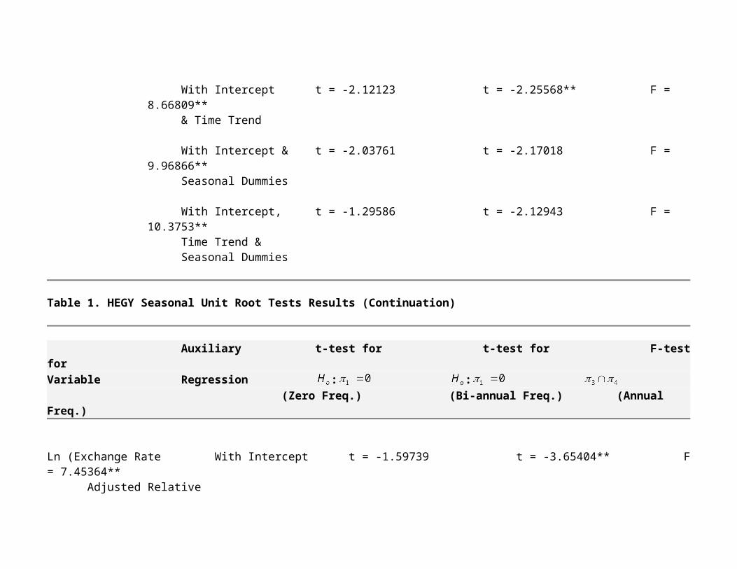
Before the specified structural models can be implemented to undertake both long run and short run analysis of the dynamics of Korean tourist arrivals, the statistical properties of the different variables will have to be investigated. Instead of undertaking the usual unit root tests on the variables of the study to ascertain departures from stationarity, seasonal unit root test via the HEGY framework is undertaken on both the dependent variable and the regressors. This analysis is necessitated by the perceived seasonal tendencies of sub-annual data used in the study particularly of the arrival series.

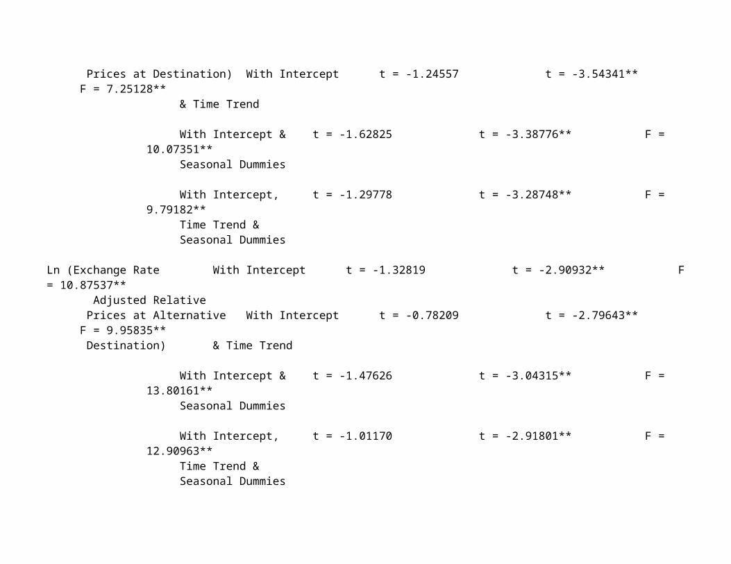
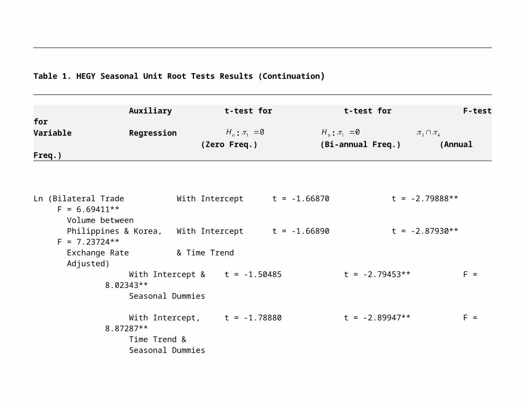
Presented in Table 1 is the outcome of implementing the HEGY Seasonal Unit Root tests of the different variables of the study. It is seen in the table that presence of unit root in the zero frequency, or in the level value of the variables in logarithmic form is empirically validated by the tests. This result indicates that all variables are non-stationary with single unit root in the zero frequency for all auxiliary regression scenarios. At the seasonal frequency however, unit roots appear to be present in three of the auxiliary regressions for Korean Tourist arrivals and in one of the auxiliary regressions for Real GDP of Korea (the one with intercept and time trend which is not a relevant scenario for this variable). All other regressors do not exhibit presence of seasonal unit roots.

Table 1. HEGY Seasonal Unit Root Tests Results

Auxiliary t-test for t-test for F-test forVariable Regression : :

(Zero Freq.) (Bi-annual Freq.) (Annual Freq.)

Ln (Korean Arrivals) With Intercept t = -1.59245 t = -1.69066 F = 4.15747**

With Intercept t = -1.04954 t = -1.67516 F = 4.14987**& Time Trend

With Intercept & t = -1.61002 t = -1.82700 F = 9.63719**Seasonal Dummies

With Intercept, t = -1.45769 t = -2.72297** F = 7.57399**Time Trend &Seasonal Dummies

Ln (Real GDP of Korea) With Intercept t = -1.35857 t = -2.20961 F = 8.97440**

With Intercept t = -2.12123 t = -2.25568** F = 8.66809**& Time Trend

With Intercept & t = -2.03761 t = -2.17018 F = 9.96866**Seasonal Dummies

With Intercept, t = -1.29586 t = -2.12943 F = 10.3753**Time Trend &Seasonal Dummies

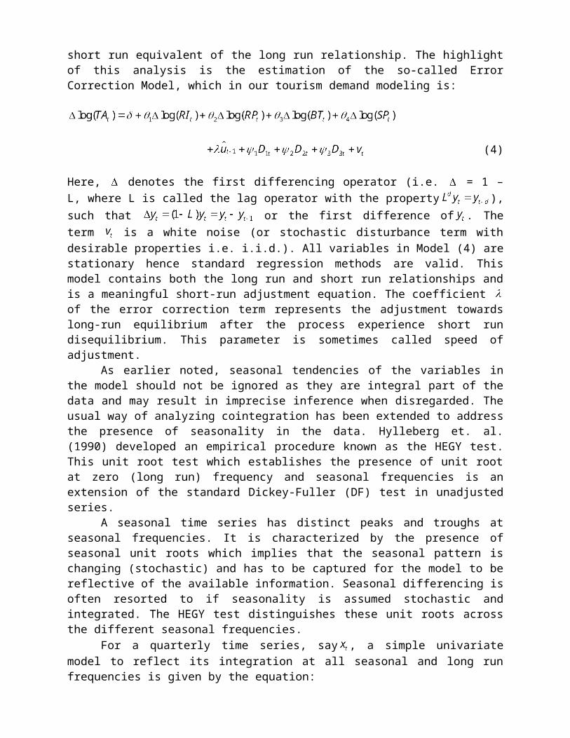
Table 1. HEGY Seasonal Unit Root Tests Results (Continuation)

Auxiliary t-test for t-test for F-test forVariable Regression : :

(Zero Freq.) (Bi-annual Freq.) (Annual Freq.)

Ln (Exchange Rate With Intercept t = -1.59739 t = -3.65404** F = 7.45364** Adjusted Relative Prices at Destination) With Intercept t = -1.24557 t = -3.54341** F = 7.25128**

& Time Trend

With Intercept & t = -1.62825 t = -3.38776** F = 10.07351**Seasonal Dummies

With Intercept, t = -1.29778 t = -3.28748** F = 9.79182**Time Trend &Seasonal Dummies

Ln (Exchange Rate With Intercept t = -1.32819 t = -2.90932** F = 10.87537** Adjusted Relative Prices at Alternative With Intercept t = -0.78209 t = -2.79643** F = 9.95835** Destination) & Time Trend

With Intercept & t = -1.47626 t = -3.04315** F = 13.80161**Seasonal Dummies

With Intercept, t = -1.01170 t = -2.91801** F = 12.90963**Time Trend &Seasonal Dummies

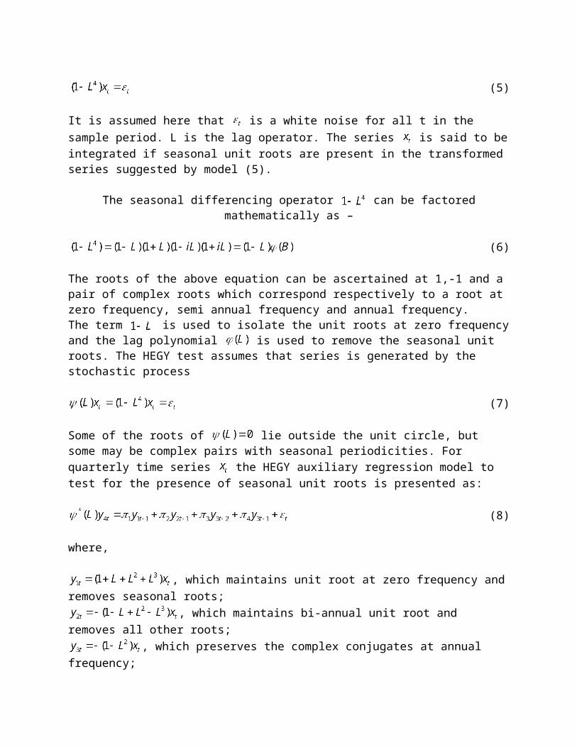
Table 1. HEGY Seasonal Unit Root Tests Results (Continuation)

Auxiliary t-test for t-test for F-test forVariable Regression : :

(Zero Freq.) (Bi-annual Freq.) (Annual Freq.)

Ln (Bilateral Trade With Intercept t = -1.66870 t = -2.79888** F = 6.69411** Volume between Philippines & Korea, With Intercept t = -1.66890 t = -2.87930** F = 7.23724** Exchange Rate & Time Trend Adjusted)

With Intercept & t = -1.50485 t = -2.79453** F = 8.02343**Seasonal Dummies

With Intercept, t = -1.78880 t = -2.89947** F = 8.87287**Time Trend &Seasonal Dummies

** Significant at 5% level

3.2 Cointegration Analysis

Since each of the logarithmic transformed variables of the study are seen to contain one unit root at the zero frequency, they are integrated of order one at that frequency, which means that they are all non-stationary at level. Regression of these variables may produce spurious results unless the variables have long-run equilibrium relationship(s), or are said to be cointegrated. In this study, two cointegration assessments will be conducted, first the multivariable cointegration procedure introduced by Johansen (1988) which features two statistical tests for cointegration – the Trace test and the Maximum Eigenvalue test, the other is the single equation procedure called the Two-Stage Augmented Engle-Granger (AEG) cointegration test ((Engle, R. F. & Granger, C.W. 1987)).

The state-of-the-art Johansen procedure not only establishes the existence of equilibrium linkage of the variables but also determines the number of cointegrating relationships (vectors) that connect the variables together. It is a VAR (Vector Auto Regression)-based procedure that requires the specification of maximum autoregressive lag order of the relationships. This maximum lag order can be empirically determined using various information criteria. The optimal lag-order is indicated when majority of the criteria suggest its use. Lag length selection in this study is implemented using the Eviews 7.2 software, the results of which are shown in Table 2 below.

When it is established that there is a single equation equilibrium linkage among the variables under study, one attractive proposition is to undertake the Augmented Engle-Granger (AEG) procedure which is anchored on the theory that if a linear combination of non-stationary variables is stationary, the variables are necessarily cointegrated. AEG is a simple 2-stage procedure, the first stage of which is running the OLS of the empirical model of the I(1) variables, then checks in the second stage whether the OLS residual is I(0) via the Augmented Dickey Fuller test.

1. Lag Length Selection of Unrestricted VAR of the Variables

The figures presented in Table 4 pertain to the empirically computed values of five information criteria used in identifying the most appropriate lag order of the unrestricted VAR model to be used in the Johansen cointegration analysis. Using a maximum lag order of 8, quarters it is established that the majority of these information criteria (three out of five) indicate one quarter to be the optimal lag length to be used in cointegration assessment. In two of these criteria, the LR and the AIC criteria, the lag order of 1 came in as close second.

Table 2. VAR Lag Order Selection Criteria

Endogenous variables:

Ln (Korean Arrivals) Ln (Real GDP of Korea)Ln (Exchange Rate Adjusted Relative Prices at Destination (Philippines))Ln (Exchange Rate Adjusted Relative Prices at Alternative Destination (Thailand)) Ln ( Exchange Rate Adjusted Bilateral Trade Between Philippines and Korea)

Sample: 1993Q1 2010Q4Included observations: 64

 Lag LogL LR FPE AIC SC HQ

0  171.2716 NA   3.81e-09 -5.195987 -5.027324 -5.1295421  460.1624  52.36145   1.00e-12* -13.44257  -12.43060*  -13.04391*2  476.9663  27.83145  1.31e-12 -13.18645 -11.33116 -12.455553  494.0231  25.58525  1.75e-12 -12.93822 -10.23962 -11.875114  534.2541   54.06048*  1.17e-12 -13.41419 -9.872275 -12.018855  554.3134  23.82035  1.54e-12 -13.25979 -8.874562 -11.532236  577.9400  24.36493  1.95e-12 -13.21687 -7.988330 -11.157097  602.4679  21.46190  2.66e-12 -13.20212 -7.130262 -10.810118  640.2818  27.17875  2.79e-12  -13.60256* -6.687384 -10.87832

*indicates lag order selected by the criterion

 LR: sequential modified LR test statistic (each test at 5% level) FPE: Final prediction error AIC: Akaike information criterion SC: Schwarz information criterion HQ: Hannan-Quinn information criterion LogL: Log Likelihood value

2. The Johansen Cointegration Tests

Having established the optimal lag length for the unrestricted VAR model, the Johansen procedure can now be implemented using EViews 7.2. Table 3 summarizes the results of the two empirical cointegration tests. Both of the tests affirm in a highly significant manner the existence of a single (i.e., rejecting the null of zero cointegrating vector and accepting the alternative of at most one, or single cointegrating vector) equilibrium relationship linking the five logarithmic transformed variables of the study. This implies that there is a unique long run equation that may appropriately be labeled as the tourism demand equation for Korean visitors to the Philippines.

Table 3. Johansen Multivariate Cointegration Tests

Rank Eigenvalue Trace test p-value - max test p-value

0 0.53551 93.710 *** [0.0001] 54.444 *** [0.0000] 1 0.25180 39.266 [0.2526] 20.596 [0.3118] 2 0.20171 18.670 [0.5274] 15.995 [0.2343] 3 0.02627 2.6745 [0.9728] 1.8904 [0.9866] 4 0.01098 0.7841 [0.3759] 0.7841 [0.3759]

Corrected for sample size (df = 62)

Rank Trace test p-value

0 93.710*** [0.0005] 1 39.266 [0.3111] 2 18.670 [0.5584] 3 2.6745 [0.9743] 4 0.78410 [0.3862]

3. The Long Run Tourism Demand Equation for Korea

As suggested by Abeysinghe (1994) due to the absence of seasonal unit roots in the model’s regressors (per HEGY’s results), the proposed long run demand model for Koreans quarterly arrivals (1.2) can now be estimated with proper augmentation of seasonal dummies. The tentative long run equation for Korean demand for Philippine international tourism is presented in (1.3). Running the Ordinary Least Squares (OLS) regression for this model results in the following estimated model:

(9)

With the following diagnostic Results:

Model Diagnostics ResultsRamsey RESET F = 0.072744, (p-value = 0.7880)Log Linearity Test = 3.27415 (p-value = 0.194549)Durbin Watson DW = 1.42524, (p-value = 0.00316808)Jarque-Bera Residual Normality = 0.419, (p-value =0.81098)ARCH Effect = 8.63676), (p-value = 0.0708486)Mean VIF for non-dummy variable Mean VIF = 8.13225CUSUM Test: Harvey-Collier t = -2.34984 (p-value 0.02193)

Based on the diagnostic assessment of the initial long run demand model, a number of empirical failures are noted. For one, the model is highly autocorrelated by virtue of the Durbin-Watson p-value of 0.00316808, and with unstable estimated parameter, suggested by the Harvey-

Collier CUSUM test with p-value of 0.02193. Marginally significant ARCH effect is also noted and a mean VIF > 6, indicative of the presence of multicollinearity. Hence, it is prudent to consider alternative long run modeling options. A number of these alternative models, mostly the original model corrected for first-order serial correlation (using different GLS procedures are presented in Table 4, which also shows the original model for comparison of parameter estimates. It may be gleaned from the table that in all of the autocorrelation corrected models, the trade volume variable becomes insignificant, leaving only Korean real GDP and exchange rate adjusted relative prices in Thailand as the only significant predictors of Korean arrivals. This finding suggests that Korean tourists to the Philippines are not price conscious at the destination and are deemed to make their travel decisions on the basis of their purchasing power and price signals from Thailand which traditionally is their top tropical tourism option.

Removing insignificant variables, the final long run demand model is the autocorrelated corrected model presented as the Prais-Winsten estimated model no. 6 in Table 4. This parsimonious representation of Korean tourism demand, presented in details as Model (10) can be assessed of its statistical and econometric properties. Presenting the empirical form of the final long-run Korean tourism demand model, the following equation emerges.

Table 4. Alternative Korean Long-Run Tourism Demand Models

Dependent variable: LN_KTOURARV (Log of Quarterly Korean Tourist Arrivals)

Regressors(1) (2) (3) (4) (5) (6)

OLS CORC HILU PWE OLS PWEConstant -8.255** -7.216** -7.219** -7.588** -5.563** -6.203**

(1.905) (2.605) (2.601) (2.560) (1.701) (2.498)LN_RINC 2.655** 2.251** 2.253** 2.253** 1.990** 1.991**

(0.2905) (0.3316) (0.3314) (0.3310) (0.1085) (0.1653)LN_RPER 0.4589 0.7561 0.7551 0.7278

(0.4551) (0.5732) (0.5726) (0.5722)LN_SPER 1.906** 1.354* 1.357* 1.360* 2.206** 2.025**

(0.5992) (0.7157) (0.7151) (0.7152) (0.2308) (0.3259)LN_TVOLER -0.2873** -0.1187 -0.1194 -0.1029

(0.1228) (0.1324) (0.1324) (0.1310)dq1 0.08561 0.08426 0.08432 0.07812 0.07338 0.06594

(0.07097) (0.05867) (0.05871) (0.05769) (0.07376) (0.05579)dq2 -0.1906** -0.2088** -0.2087** -0.2100** -0.2172** -0.2194**

(0.07178) (0.06508) (0.06511) (0.06470) (0.07369) (0.06209)dq3 -0.02285 -0.03222 -0.03218 -0.03170 -0.04175 -0.03863

(0.07118) (0.05779) (0.05783) (0.05739) (0.07375) (0.05526)T 72 71 71 72 72 72

Adj. R2 0.8974 0.9042 0.9042 0.9071 0.8886 0.9070lnL 13.76 9.682

Standard errors in parentheses* indicates significance at the 10 percent level** indicates significance at the 5 percent level

*** indicates significance at the 1 percent levelOLS – Ordinary Least SquaresCORC – Cochrane-Orcutt Iterative GLS ProcedureHILU – Hildreth-Lu Grid Search GLS ProcedurePWE – Prais-Winsten GLS Estimation ProcedureGLS – Generalized Least Squares

(0.0156)*** (2.55e-18)*** (3.94e-08)*** (0.242) (0.008)*** (0.487) (10)

0.9070 2.107 = 0.426467

(p-values in parentheses)

Model Diagnostics ResultsRamsey RESET F = 0.252507, (p-value = 0.6170)Log Linearity Test: = 0.000767055, (p-value = 0.977905)Durbin Watson: DW = 2.107, (p-value = 0.4174)Jarque-Bera Residual Normality: = 0.962, (p-value =0.61829)ARCH Effect: = 2.96012 (p–value =.5645)Mean VIF for non-dummy variable Mean VIF = 1.0730CUSUM Test: Harvey-Collier t = -1.46373, (p-value 0.1481)

4. The Short-Run Error Correction Model

The residual of the above statistically and econometrically adequate long-run model is extracted, and the one-period lagged value of which is introduced as additional regressor to the short-run model to produce an Error Correction model presented in Table 5. The coefficient of this error correction term in the model is equivalent to the speed of adjustment, which in this case is extremely significant statistically (p<0.0001), with a magnitude of -0.70262. When interpreted, this figure is equivalent to the proportion (70.26%) by which deviations from equilibrium tourism arrivals will be corrected within a quarter.

Table 5. Error Correction Model (ECM) – Short Run Dynamics

Dependent variable: Var. Coefficient Std. Error t-ratio p-value Sig.

const -0.00404 0.0497684 -0.0813 0.93549 ns 5.07065 1.6586 3.0572 0.00326 *** 1.07334 0.539637 1.9890 0.05098 * 0.03790 0.0650257 0.5829 0.56204 ns -0.33203 0.0645717 -5.1421 <0.00001 *** 0.15601 0.0661545 2.3583 0.02142 ** -0.70262 0.127983 -5.4900 <0.00001 ***

* indicates significance at the 10 percent level** indicates significance at the 5 percent level*** indicates significance at the 1 percent levelns – not significant

Diagnostics:

RESET test for specification - Null hypothesis: specification is adequate Test statistic: F(1, 63) = 0.526906 with p-value = 0.470599Jarque-Bera test for normality of residual - Null hypothesis: error is normally distributed Test statistic: Chi-square(2) = 8.29825 with p-value = 0.0157782Test for ARCH of order 1 - Null hypothesis: no ARCH effect is present Test statistic: LM = 1.84215 with p-value = 0.764762LM test for autocorrelation up to order 1 - Null hypothesis: no autocorrelation Test statistic: LMF = 0.125862 with p-value = 0.723946CUSUM test for parameter stability - Null hypothesis: no change in parameters Test statistic: Harvey-Collier t(63) = -0.224889 with p-value = 0.822793

Evaluation of the diagnostic results of the short-run Error Correction model reveals its relative adequacy. The only departure from model’s sufficiency is the residual normality diagnostic with a p-value of 0.01578 (p<0.05). The estimated coefficients of the short-run model are interpreted as short-run elasticities, hence, in the short-run Koreans are extremely sensitive to their financial capability in making their travel decisions to the Philippines (as evidenced by the short-run income elasticity of 5.07 (compared to long-run income elasticity of 1.99) but almost unitary elastic to price signals from their alternative destination Thailand, with substitution elasticity of 1.07 (compared to the estimated long run substitution elasticity of 2.03). Highly significant seasonal components of the short run model are also noted.

3.3 Concluding Remarks and Policy Implications

This study aims to evaluate econometrically the modern phenomenon of massive inflow of Korean tourists to the Philippines. Long run and short run analysis of are conducted using relevant quarterly data and the double logarithmic functional specification to produce reliable estimates of tourism elasticities important in planning. Seasonality assessment of the Korean tourism inflow is also conducted to check whether this recurring time series component should be incorporated in both the long run and the short run model, to avoid some form of omitted variable bias.

The study uncovers a unique long run equilibrium Korean tourism demand model whose significant regressors are the Real GDP of Korea and the exchange rate adjusted price ratio at the alternative destination (which is Thailand – substitute destination). The price ratio at the destination, adjusted for the effect of exchange rate variations (which proxies for the cost of living at the destination) proved to be inconsequential, and so with the exchange rate adjusted bilateral trade of Philippines and Korea (which represent the economic activity of business travelers). This result implies that Korean tourists are not price conscious at the destination (a good signal indeed for local businesses catering to Korean tourists) but are sensitive to price signals from Thailand. The insignificance of the trade variable may imply the crowding out of business travelers by pleasure and special interest groups of Korean tourists.

Tourism demand from the Korean market is shown to be highly income elastic. The magnitudes of both the short run and long run income elasticity of demand of 1.99 and 5.07 respectively accentuate the importance of Korea’s economic performance to the inflow of Korean tourists to the Philippines; a well performing Korean economy augurs well for the Philippines tourism sector. The long run price elasticity at the substitute destination of 2.025 and the corresponding short run elasticity of 1.0733 highlight the stiff competition between the Philippines and Thailand in attracting Korean tourists.

With Korea’s Real GDP expected to grow 2.8% in 2013 from 2.0% in 2012 (Samsung Economic Research Institute (2013)) and Thailand’s inflation to increase to 3.3 in 2013 from 3.2 in the previous year (Asian Development Outlook 2012 Update (October 2012)), the massive inflows of Korean tourists to the Philippines will continue. Hence, in anticipation of heavier volume of Korean arrivals, it would be prudent for the government and the private sector to craft focused promotional programs, logistical and infrastructure policies and plans, tax breaks, manpower distribution and positioning, among other important undertakings.

The stable seasonality of Korean tourism to the Philippines as revealed by both the long run and short run models indicates the need for careful planning in anticipation of the lean and peak arrival quarters. The significant dip during the second quarter and the spikes in arrivals in the other quarters may result in inefficient use of resources if not carefully planned for. The stability of the equilibrium (long run) model may be gleaned from the very high adjustment speed of 70.26 percent, implying that adjustment to equilibrium occur almost instantaneously within a quarter - suggestive of more predictable quarterly volume of tourists which is conducive to accurate planning.

5. ACKNOWLEDGEMENTS

The author would like to extend his deep appreciation of the Angelo King Institute for the funding support under the AKI Research Grant Program for 2012. Research assistance of Paula Arnedo and Gio Dalisay is also appreciated.6. REFERENCES

Abeysinghe, T. (1994). Deterministic seasonal models and spurious regressions. Journal of Econometrics 61, 259-272.

Asian Development Bank (2012). Asian Development Outlook October 2012 UpdateDepartment of Tourism. (2008). Philippine Tourism: Stable amidst a global tourism downturn.

Philippine Department of Tourism. Tourism Statistics ArchivesDepartment of Tourism (2012a). Tourism Statistics. http://www.tourism.gov.ph/Department of Tourism. (2012b). Visitor Arrivals Increased by 9.78% from January to August

2012. Tourism Statistics. Retrieved from http://www.tourism.gov.ph/Pages/Industry Performance.aspx

Engle, R.F. & Granger, C.W (1987). Cointegration and Error Correction Representation, Estimation and Testing. Econometrica 55(2), 251-276

Hicap, J. (2009, September 13). Koreans Flock to the Philippines to Learn English. Korea Times. Retrieved from http://www.koreatimes.co.kr/www/news/nation/2009/09/117_51729.html

Hylleberg, S., Engle, R. & Granger, C.W. (1990). Seasonal Integration and Cointegration. Journal of Econometrics 44, 215-238.

Johansen, S. (1988). A Statistical Analysis of Cointegration Vectors. Journal of Economic Dynamics and Control 12, 231-254.

Kulendran, N. (1996). Modeling quarterly tourism flows to Australia. Tourism Economics 2, 203-222.

Kulendran, N and M. King (1997). Forecasting international quarterly flows using error correction and time series models. International Journal of Forecasting 13, 319-327.

Lim, C. (1997). Review of international tourism demand models. Annals of Tourism Research 24, 835-849

Lim, C. and M. McAleer (2001). Cointegration analysis of quarterly tourism demand by Hongkong and Singapore to Australia. Applied Economics 33, 1599-1619

Narayan, P.K. (2004). Fuji’s tourism demand: the ARDL approach to Cointegration. Tourism Economics 10(2), 193-206

Samsung Economic Research Institute (2013). Korea Economic Trends Vol. 18, No. 3 Jan. 21, 2013, SERI World.org

Song, H. and S.F. Witt (2000). Tourism Demand Modeling and Forecasting: Modern Econometric Approaches. Pergamon: Oxford.

Song, H., S.F. Witt and Gang Li (2003). Modelling and forecasting the demand for Thai tourism. Tourism Economics 9(4), 363-387

Song, H., K.F. Wong, and K. Chon (2003). Modeling and Forecasting the Demand for Hong Kong Tourism. International Journal of Hospitality Management 22, 435-451.

Stock, J. & Watson, M. (2007). Introduction to Econometrics, 2nd Edition. Pearson-Addison Wesley, Boston.

Turner, L. W. and S.F. Witt (2001a) Factors influencing demand for international tourism: tourism demand analysis using structural equation modeling, revisited. Tourism Economics 7 (1), 21-38.

Turner, L. W. and S.F. Witt (2001b). Forecasting tourism using univariate and multivariate structural time series models. Tourism Economics 7 (2), 135-147.