doc.lagout.org Science/2... · · 2016-05-08Undergraduate Topics in Computer Science (UTiCS)...
338
Transcript of doc.lagout.org Science/2... · · 2016-05-08Undergraduate Topics in Computer Science (UTiCS)...


Undergraduate Topics in Computer Science

Undergraduate Topics in Computer Science (UTiCS) delivers high-quality instructional content forundergraduates studying in all areas of computing and information science. From core foundationaland theoretical material to final-year topics and applications, UTiCS books take a fresh, concise, andmodern approach and are ideal for self-study or for a one- or two-semester course. The texts areall authored by established experts in their fields, reviewed by an international advisory board, andcontain numerous examples and problems. Many include fully worked solutions.
For further volumes:www.springer.com/series/7592

Michael Oberguggenberger �
Alexander Ostermann
Analysis forComputerScientists
Foundations, Methods, andAlgorithms
Translated in collaboration with Elisabeth Bradley

Michael OberguggenbergerInstitute of Basic Sciences in Civil EngUniversity of InnsbruckTechnikerstrasse 13Innsbruck [email protected]
Alexander OstermannDepartment of MathematicsUniversity of InnsbruckTechnikerstrasse 13/7Innsbruck [email protected]
Series editorIan Mackie
Advisory boardSamson Abramsky, University of Oxford, Oxford, UKKarin Breitman, Pontifical Catholic University of Rio de Janeiro, Rio de Janeiro, BrazilChris Hankin, Imperial College London, London, UKDexter Kozen, Cornell University, Ithaca, USAAndrew Pitts, University of Cambridge, Cambridge, UKHanne Riis Nielson, Technical University of Denmark, Kongens Lyngby, DenmarkSteven Skiena, Stony Brook University, Stony Brook, USAIain Stewart, University of Durham, Durham, UK
ISSN 1863-7310ISBN 978-0-85729-445-6 e-ISBN 978-0-85729-446-3DOI 10.1007/978-0-85729-446-3Springer London Dordrecht Heidelberg New York
British Library Cataloguing in Publication DataA catalogue record for this book is available from the British Library
Library of Congress Control Number: 2011924489
© Springer-Verlag London Limited 2011Apart from any fair dealing for the purposes of research or private study, or criticism or review, as per-mitted under the Copyright, Designs and Patents Act 1988, this publication may only be reproduced,stored or transmitted, in any form or by any means, with the prior permission in writing of the publish-ers, or in the case of reprographic reproduction in accordance with the terms of licenses issued by theCopyright Licensing Agency. Enquiries concerning reproduction outside those terms should be sent tothe publishers.The use of registered names, trademarks, etc., in this publication does not imply, even in the absence of aspecific statement, that such names are exempt from the relevant laws and regulations and therefore freefor general use.The publisher makes no representation, express or implied, with regard to the accuracy of the informationcontained in this book and cannot accept any legal responsibility or liability for any errors or omissionsthat may be made.
Cover design: VTeX UAB, Lithuania
Printed on acid-free paper
Springer is part of Springer Science+Business Media (www.springer.com)

Preface
Mathematics and mathematical modelling are of central importance in computer sci-ence. For this reason the teaching concepts of mathematics in computer science haveto be constantly reconsidered, and the choice of material and the motivation have tobe adapted. This applies in particular to mathematical analysis, whose significancehas to be conveyed in an environment where thinking in discrete structures is pre-dominant. On the one hand, an analysis course in computer science has to cover theessential basic knowledge. On the other hand, it has to convey the importance ofmathematical analysis in applications, especially those which will be encounteredby computer scientists in their professional life.
We see a need to renew the didactic principles of mathematics teaching in com-puter science, and to restructure the teaching according to contemporary require-ments. We try to address this situation with this textbook, which we have developedbased on the following concepts:1. An algorithmic approach.2. A concise presentation.3. Integrating mathematical software as an important component.4. Emphasis on modelling and applications of analysis.The book is positioned in the triangle between mathematics, computer science andapplications. In this field, algorithmic thinking is of high importance. The algorith-mic approach chosen by us encompasses:(a) Development of concepts of analysis from an algorithmic point of view.(b) Illustrations and explanations using MATLAB and maple programs as well as
Java applets.(c) Computer experiments and programming exercises as motivation for actively
acquiring the subject matter.(d) Mathematical theory combined with basic concepts and methods of numerical
analysis.Concise presentation means for us that we have deliberately reduced the subject
matter to the essential ideas. For example, we do not discuss the general convergencetheory of power series; however, we do outline Taylor expansion with an estimate ofthe remainder term. (Taylor expansion is included in the book as it is an indispens-able tool for modelling and numerical analysis.) For the sake of readability, proofsare only detailed in the main text if they introduce essential ideas and contribute tothe understanding of the concepts. To continue with the example above, the integral
v
vi Preface
representation of the remainder term of the Taylor expansion is derived by integra-tion by parts. In contrast, Lagrange’s form of the remainder term, which requires themean value theorem of integration, is only mentioned. Nevertheless we have put ef-fort into ensuring a self-contained presentation. We assign a high value to geometricintuition, which is reflected in the large number of illustrations.
Due to the terse presentation it was possible to cover the whole spectrum fromfoundations to interesting applications of analysis (again selected from the view-point of computer science), such as fractals, L-systems, curves and surfaces, linearregression, differential equations and dynamical systems. These topics give suffi-cient opportunity to enter various aspects of mathematical modelling.
The present book is a translation of the original German version that appearedin 2005 (with a second edition in 2009). We have kept the structure of the Germantext, but we took the opportunity to improve the presentation at various places.
The contents of the book are as follows. Chapters 1–8, 10–12 and 14–17 aredevoted to the basic concepts of analysis, Chapters 9, 13 and 18–21 are dedicated toimportant applications and more advanced topics. Appendices A and B collect sometools from vector and matrix algebra, and Appendix C supplies further details, whichwere deliberately omitted in the main text. The employed software, which is anintegral part of our concept, is summarised in Appendix D. Each chapter is precededby a brief introduction for orientation. The text is enriched by computer experimentswhich should encourage the reader to actively acquire the subject matter. Finally,every chapter has exercises, half of which are to be solved with the help of computerprograms. The book can be used from the first semester on as the main textbook fora course, as a complementary text, or for self-study.
We thank Elisabeth Bradley for her help in the translation of the text. Further, wethank the editors of Springer, especially Simon Rees and Wayne Wheeler, for theirsupport and advice during the preparation of the English text.
Michael OberguggenbergerAlexander Ostermann
InnsbruckMarch 2011

Contents
1 Numbers . . . . . . . . . . . . . . . . . . . . . . . . . . . . . . . . . . 11.1 The Real Numbers . . . . . . . . . . . . . . . . . . . . . . . . . . 11.2 Order Relation and Arithmetic on R . . . . . . . . . . . . . . . . . 51.3 Machine Numbers . . . . . . . . . . . . . . . . . . . . . . . . . . 81.4 Rounding . . . . . . . . . . . . . . . . . . . . . . . . . . . . . . . 101.5 Exercises . . . . . . . . . . . . . . . . . . . . . . . . . . . . . . . 11
2 Real-Valued Functions . . . . . . . . . . . . . . . . . . . . . . . . . . 132.1 Basic Notions . . . . . . . . . . . . . . . . . . . . . . . . . . . . 132.2 Some Elementary Functions . . . . . . . . . . . . . . . . . . . . . 172.3 Exercises . . . . . . . . . . . . . . . . . . . . . . . . . . . . . . . 22
3 Trigonometry . . . . . . . . . . . . . . . . . . . . . . . . . . . . . . . 253.1 Trigonometric Functions at the Triangle . . . . . . . . . . . . . . . 253.2 Extension of the Trigonometric Functions to R . . . . . . . . . . . 293.3 Cyclometric Functions . . . . . . . . . . . . . . . . . . . . . . . . 313.4 Exercises . . . . . . . . . . . . . . . . . . . . . . . . . . . . . . . 34
4 Complex Numbers . . . . . . . . . . . . . . . . . . . . . . . . . . . . 374.1 The Notion of Complex Numbers . . . . . . . . . . . . . . . . . . 374.2 The Complex Exponential Function . . . . . . . . . . . . . . . . . 404.3 Mapping Properties of Complex Functions . . . . . . . . . . . . . 414.4 Exercises . . . . . . . . . . . . . . . . . . . . . . . . . . . . . . . 43
5 Sequences and Series . . . . . . . . . . . . . . . . . . . . . . . . . . . 455.1 The Notion of an Infinite Sequence . . . . . . . . . . . . . . . . . 455.2 The Completeness of the Set of Real Numbers . . . . . . . . . . . 515.3 Infinite Series . . . . . . . . . . . . . . . . . . . . . . . . . . . . 535.4 Supplement: Accumulation Points of Sequences . . . . . . . . . . 575.5 Exercises . . . . . . . . . . . . . . . . . . . . . . . . . . . . . . . 60
6 Limits and Continuity of Functions . . . . . . . . . . . . . . . . . . . 636.1 The Notion of Continuity . . . . . . . . . . . . . . . . . . . . . . 636.2 Trigonometric Limits . . . . . . . . . . . . . . . . . . . . . . . . 676.3 Zeros of Continuous Functions . . . . . . . . . . . . . . . . . . . 686.4 Exercises . . . . . . . . . . . . . . . . . . . . . . . . . . . . . . . 71
vii

viii Contents
7 The Derivative of a Function . . . . . . . . . . . . . . . . . . . . . . . 737.1 Motivation . . . . . . . . . . . . . . . . . . . . . . . . . . . . . . 737.2 The Derivative . . . . . . . . . . . . . . . . . . . . . . . . . . . . 757.3 Interpretations of the Derivative . . . . . . . . . . . . . . . . . . . 797.4 Differentiation Rules . . . . . . . . . . . . . . . . . . . . . . . . . 827.5 Numerical Differentiation . . . . . . . . . . . . . . . . . . . . . . 877.6 Exercises . . . . . . . . . . . . . . . . . . . . . . . . . . . . . . . 92
8 Applications of the Derivative . . . . . . . . . . . . . . . . . . . . . . 958.1 Curve Sketching . . . . . . . . . . . . . . . . . . . . . . . . . . . 958.2 Newton’s Method . . . . . . . . . . . . . . . . . . . . . . . . . . 1008.3 Regression Line Through the Origin . . . . . . . . . . . . . . . . 1058.4 Exercises . . . . . . . . . . . . . . . . . . . . . . . . . . . . . . . 108
9 Fractals and L-Systems . . . . . . . . . . . . . . . . . . . . . . . . . 1119.1 Fractals . . . . . . . . . . . . . . . . . . . . . . . . . . . . . . . . 1119.2 Mandelbrot Sets . . . . . . . . . . . . . . . . . . . . . . . . . . . 1179.3 Julia Sets . . . . . . . . . . . . . . . . . . . . . . . . . . . . . . . 1199.4 Newton’s Method in C . . . . . . . . . . . . . . . . . . . . . . . . 1209.5 L-Systems . . . . . . . . . . . . . . . . . . . . . . . . . . . . . . 1229.6 Exercises . . . . . . . . . . . . . . . . . . . . . . . . . . . . . . . 125
10 Antiderivatives . . . . . . . . . . . . . . . . . . . . . . . . . . . . . . 12710.1 Indefinite Integrals . . . . . . . . . . . . . . . . . . . . . . . . . . 12710.2 Integration Formulae . . . . . . . . . . . . . . . . . . . . . . . . . 13010.3 Exercises . . . . . . . . . . . . . . . . . . . . . . . . . . . . . . . 133
11 Definite Integrals . . . . . . . . . . . . . . . . . . . . . . . . . . . . . 13511.1 The Riemann Integral . . . . . . . . . . . . . . . . . . . . . . . . 13511.2 Fundamental Theorems of Calculus . . . . . . . . . . . . . . . . . 14111.3 Applications of the Definite Integral . . . . . . . . . . . . . . . . . 14311.4 Exercises . . . . . . . . . . . . . . . . . . . . . . . . . . . . . . . 146
12 Taylor Series . . . . . . . . . . . . . . . . . . . . . . . . . . . . . . . 14912.1 Taylor’s Formula . . . . . . . . . . . . . . . . . . . . . . . . . . . 14912.2 Taylor’s Theorem . . . . . . . . . . . . . . . . . . . . . . . . . . 15312.3 Applications of Taylor’s Formula . . . . . . . . . . . . . . . . . . 15412.4 Exercises . . . . . . . . . . . . . . . . . . . . . . . . . . . . . . . 157
13 Numerical Integration . . . . . . . . . . . . . . . . . . . . . . . . . . 15913.1 Quadrature Formulae . . . . . . . . . . . . . . . . . . . . . . . . 15913.2 Accuracy and Efficiency . . . . . . . . . . . . . . . . . . . . . . . 16413.3 Exercises . . . . . . . . . . . . . . . . . . . . . . . . . . . . . . . 166
14 Curves . . . . . . . . . . . . . . . . . . . . . . . . . . . . . . . . . . . 16914.1 Parametrised Curves in the Plane . . . . . . . . . . . . . . . . . . 16914.2 Arc Length and Curvature . . . . . . . . . . . . . . . . . . . . . . 17714.3 Plane Curves in Polar Coordinates . . . . . . . . . . . . . . . . . 183

Contents ix
14.4 Parametrised Space Curves . . . . . . . . . . . . . . . . . . . . . 18514.5 Exercises . . . . . . . . . . . . . . . . . . . . . . . . . . . . . . . 187
15 Scalar-Valued Functions of Two Variables . . . . . . . . . . . . . . . 19115.1 Graph and Partial Mappings . . . . . . . . . . . . . . . . . . . . . 19115.2 Continuity . . . . . . . . . . . . . . . . . . . . . . . . . . . . . . 19315.3 Partial Derivatives . . . . . . . . . . . . . . . . . . . . . . . . . . 19415.4 The Fréchet Derivative . . . . . . . . . . . . . . . . . . . . . . . . 19815.5 Directional Derivative and Gradient . . . . . . . . . . . . . . . . . 20215.6 The Taylor Formula in Two Variables . . . . . . . . . . . . . . . . 20415.7 Local Maxima and Minima . . . . . . . . . . . . . . . . . . . . . 20615.8 Exercises . . . . . . . . . . . . . . . . . . . . . . . . . . . . . . . 209
16 Vector-Valued Functions of Two Variables . . . . . . . . . . . . . . . 21116.1 Vector Fields and the Jacobian . . . . . . . . . . . . . . . . . . . . 21116.2 Newton’s Method in Two Variables . . . . . . . . . . . . . . . . . 21316.3 Parametric Surfaces . . . . . . . . . . . . . . . . . . . . . . . . . 21516.4 Exercises . . . . . . . . . . . . . . . . . . . . . . . . . . . . . . . 217
17 Integration of Functions of Two Variables . . . . . . . . . . . . . . . 21917.1 Double Integrals . . . . . . . . . . . . . . . . . . . . . . . . . . . 21917.2 Applications of the Double Integral . . . . . . . . . . . . . . . . . 22517.3 The Transformation Formula . . . . . . . . . . . . . . . . . . . . 22717.4 Exercises . . . . . . . . . . . . . . . . . . . . . . . . . . . . . . . 230
18 Linear Regression . . . . . . . . . . . . . . . . . . . . . . . . . . . . 23318.1 Simple Linear Regression . . . . . . . . . . . . . . . . . . . . . . 23318.2 Rudiments of the Analysis of Variance . . . . . . . . . . . . . . . 23918.3 Multiple Linear Regression . . . . . . . . . . . . . . . . . . . . . 24218.4 Model Fitting and Variable Selection . . . . . . . . . . . . . . . . 24518.5 Exercises . . . . . . . . . . . . . . . . . . . . . . . . . . . . . . . 249
19 Differential Equations . . . . . . . . . . . . . . . . . . . . . . . . . . 25119.1 Initial Value Problems . . . . . . . . . . . . . . . . . . . . . . . . 25119.2 First-Order Linear Differential Equations . . . . . . . . . . . . . . 25319.3 Existence and Uniqueness of the Solution . . . . . . . . . . . . . . 25919.4 Method of Power Series . . . . . . . . . . . . . . . . . . . . . . . 26219.5 Qualitative Theory . . . . . . . . . . . . . . . . . . . . . . . . . . 26419.6 Exercises . . . . . . . . . . . . . . . . . . . . . . . . . . . . . . . 266
20 Systems of Differential Equations . . . . . . . . . . . . . . . . . . . . 26720.1 Systems of Linear Differential Equations . . . . . . . . . . . . . . 26720.2 Systems of Nonlinear Differential Equations . . . . . . . . . . . . 27820.3 Exercises . . . . . . . . . . . . . . . . . . . . . . . . . . . . . . . 283
21 Numerical Solution of Differential Equations . . . . . . . . . . . . . 28721.1 The Explicit Euler Method . . . . . . . . . . . . . . . . . . . . . . 28721.2 Stability and Stiff Problems . . . . . . . . . . . . . . . . . . . . . 290

x Contents
21.3 Systems of Differential Equations . . . . . . . . . . . . . . . . . . 29221.4 Exercises . . . . . . . . . . . . . . . . . . . . . . . . . . . . . . . 293
22 Appendix A: Vector Algebra . . . . . . . . . . . . . . . . . . . . . . 29522.1 Cartesian Coordinate Systems . . . . . . . . . . . . . . . . . . . . 29522.2 Vectors . . . . . . . . . . . . . . . . . . . . . . . . . . . . . . . . 29522.3 Vectors in a Cartesian Coordinate System . . . . . . . . . . . . . . 29622.4 The Inner Product (Dot Product) . . . . . . . . . . . . . . . . . . 29922.5 The Outer Product (Cross Product) . . . . . . . . . . . . . . . . . 30022.6 Straight Lines in the Plane . . . . . . . . . . . . . . . . . . . . . . 30122.7 Planes in Space . . . . . . . . . . . . . . . . . . . . . . . . . . . 30322.8 Straight Lines in Space . . . . . . . . . . . . . . . . . . . . . . . 304
23 Appendix B: Matrices . . . . . . . . . . . . . . . . . . . . . . . . . . 30723.1 Matrix Algebra . . . . . . . . . . . . . . . . . . . . . . . . . . . . 30723.2 Canonical Form of Matrices . . . . . . . . . . . . . . . . . . . . . 311
24 Appendix C: Further Results on Continuity . . . . . . . . . . . . . . 31724.1 Continuity of the Inverse Function . . . . . . . . . . . . . . . . . 31724.2 Limits of Sequences of Functions . . . . . . . . . . . . . . . . . . 31824.3 The Exponential Series . . . . . . . . . . . . . . . . . . . . . . . 32024.4 Lipschitz Continuity and Uniform Continuity . . . . . . . . . . . . 325
25 Appendix D: Description of the Supplementary Software . . . . . . 329
References . . . . . . . . . . . . . . . . . . . . . . . . . . . . . . . . . . . 331
Index . . . . . . . . . . . . . . . . . . . . . . . . . . . . . . . . . . . . . . 333

1Numbers
The commonly known rational numbers (fractions) are not sufficient for a rigorousfoundation of mathematical analysis. The historical development shows that for is-sues concerning analysis, the rational numbers have to be extended to the real num-bers. For clarity we introduce the real numbers as decimal numbers with an infinitenumber of decimal places. We illustrate exemplarily how the rules of calculationand the order relation extend from the rational to the real numbers in a natural way.
A further section is dedicated to floating point numbers, which are implementedin most programming languages as approximations to the real numbers. In partic-ular, we will discuss optimal rounding and in connection with this the relative ma-chine accuracy.
1.1 The Real Numbers
In this book we assume the following number systems as known:
N = {1,2,3,4, . . .} the set of natural numbers;N0 = N ∪ {0} the set of natural numbers including zero;Z = {. . . ,−3,−2,−1,0,1,2,3, . . .} the set of integers;
Q ={
k
n; k ∈ Z and n ∈ N
}the set of rational numbers.
Two rational numbers kn
and �m
are equal if and only if km = �n. Further, an integerk ∈ Z can be identified with the fraction k
1 ∈ Q. Consequently, the inclusions N ⊂Z ⊂ Q are true.
M. Oberguggenberger, A. Ostermann, Analysis for Computer Scientists,Undergraduate Topics in Computer Science,DOI 10.1007/978-0-85729-446-3_1, © Springer-Verlag London Limited 2011
1

2 1 Numbers
Fig. 1.1 The real line
Let M and N be arbitrary sets. A mapping from M to N is a rule which assignsto each element in M exactly one element in N .1 A mapping is called bijective, iffor each element n ∈ N there exists exactly one element in M which is assignedto n.
Definition 1.1 Two sets M and N have the same cardinality if there exists a bijec-tive mapping between these sets. A set M is called countably infinite if it has thesame cardinality as N.
The sets N, Z and Q have the same cardinality and in this sense are equally large.All three sets have an infinite number of elements which can be enumerated. Eachenumeration represents a bijective mapping to N. The countability of Z can be seenfrom the representation Z = {0,1,−1,2,−2,3,−3, . . .}. To prove the countabilityof Q, Cantor’s2 diagonal method is used:
11 → 2
131 → 4
1 . . .
↙ ↗ ↙12
22
32
42 . . .
↓ ↗ ↙13
23
33
43 . . .
↙14
24
34
44 . . .
......
......
The enumeration is carried out in the direction of the arrows, where each rationalnumber is only counted at its first appearance. In this way the countability of allpositive rational number (and therefore all rational numbers) is proven.
To visualise the rational numbers we use a line, which can be pictured as aninfinitely long ruler, on which an arbitrary point is labelled as zero. The integers aremarked equidistantly starting from zero. Likewise each rational number is allocateda specific place on the real line according to its size; see Fig. 1.1.
However, the real line also contains points which do not correspond to rationalnumbers. (We say that Q is not complete.) For instance, the length of the diagonal d
in the unit square (see Fig. 1.2) can be measured with a ruler. Yet, the Pythagoreansalready knew that d2 = 2, but that d = √
2 is not a rational number.
1We will rarely use the term mapping in such generality. The special case of real-valued functions,which is important for us, will be discussed thoroughly in Chap. 2.2G. Cantor, 1845–1918.

1.1 The Real Numbers 3
Fig. 1.2 Diagonal in the unitsquare
Proposition 1.2√
2 /∈ Q.
Proof This statement is proven indirectly. Assume that√
2 were rational. Then√
2can be represented as a reduced fraction
√2 = k
n∈ Q. Squaring this equation gives
k2 = 2n2 and thus k2 would be an even number. This is only possible if k itself isan even number, so k = 2l. If we substitute this into the above we obtain 4l2 = 2n2
which simplifies to 2l2 = n2. Consequently n would also be even which is in con-tradiction to the initial assumption that the fraction k
nwas reduced. �
As is generally known,√
2 is the unique positive root of the polynomial x2 − 2.The naive supposition that all non-rational numbers are roots of polynomials withinteger coefficients turns out to be incorrect. There are other non-rational numbers(so-called transcendental numbers) which cannot be represented in this way. Forexample, the ratio of a circle’s circumference to its diameter,
π = 3.141592653589793 . . . /∈ Q,
is transcendental, but it can be represented on the real line as half the circumferenceof the circle with radius 1 (e.g. through unwinding).
In the following we will take up a pragmatic point of view and construct themissing numbers as decimals.
Definition 1.3 A finite decimal number x with l decimal places has the form
x = ±d0.d1d2d3 . . . dl
with d0 ∈ N0 and the single digits di ∈ {0,1, . . . ,9}, 1 ≤ i ≤ l, with dl �= 0.
Proposition 1.4 (Representing rational numbers as decimals) Each rational num-ber can be written as a finite or periodic decimal.
Proof Let q ∈ Q and consequently q = kn
with k ∈ Z and n ∈ N. One obtains therepresentation of q as a decimal by successive division with remainder. Since theremainder r ∈ N always fulfils the condition 0 ≤ r < n, the remainder will be zeroor periodic after a maximum of n iterations. �
Example 1.5 Let us take q = − 57 ∈ Q as an example. Successive division with
remainder shows that q = −0.71428571428571 . . . with remainders 5,1,3,2,6,4,5,1,3,2,6,4,5,1,3, . . . The period of this decimal is six.
4 1 Numbers
Each non-zero decimal with a finite number of decimal places can be written asa periodic decimal (with an infinite number of decimal places). To this end onediminishes the last non-zero digit by one and then fills the remaining infinitelymany decimal places with the digit 9. For example, the fraction − 17
50 = −0.34 =−0.3399999 . . . becomes periodic after the third decimal place. In this way Q canbe considered as the set of all decimals which turn periodic from a certain numberof decimal places onwards.
Definition 1.6 The set of real numbers R consists of all decimals of the form
±d0.d1d2d3 . . .
with d0 ∈ N0 and digits di ∈ {0, . . . ,9}, i.e., decimals with an infinite number ofdecimal places. The set R \ Q is called the set of irrational numbers.
Obviously Q ⊂ R. According to what was mentioned so far the numbers
0.1010010001000010 . . . and√
2
are irrational. There are much more irrational than rational numbers, as is shown bythe following proposition.
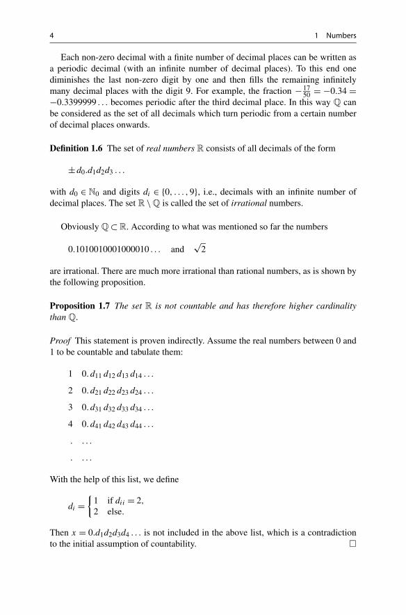
Proposition 1.7 The set R is not countable and has therefore higher cardinalitythan Q.
Proof This statement is proven indirectly. Assume the real numbers between 0 and1 to be countable and tabulate them:
1 0. d11 d12 d13 d14 . . .
2 0. d21 d22 d23 d24 . . .
3 0. d31 d32 d33 d34 . . .
4 0. d41 d42 d43 d44 . . .
. . . .
. . . .
With the help of this list, we define
di ={
1 if dii = 2,
2 else.
Then x = 0.d1d2d3d4 . . . is not included in the above list, which is a contradictionto the initial assumption of countability. �

6 1 Numbers
The relation ≤ obviously has the following properties. For all a, b, c ∈ R one has
a ≤ a (reflexivity),
a ≤ b and b ≤ c ⇒ a ≤ c (transitivity),
a ≤ b and b ≤ a ⇒ a = b (antisymmetry).
In case of a ≤ b and a �= b one writes a < b and calls a less than b. Furthermore,one defines a ≥ b, if b ≤ a (in words: a greater than or equal to b), and a > b, ifb < a (in words: a greater than b).
Addition and multiplication can be carried over from Q to R in a similar way.Graphically one uses the fact that each real number corresponds to a segment onthe real line. One thus defines the addition of real numbers as the addition of therespective segments.
A rigorous and at the same time algorithmic definition of the addition starts fromthe observation that real numbers can be approximated by rational numbers to anydegree of accuracy. Let a = a0.a1a2 . . . and b = b0.b1b2 . . . be two non-negative realnumbers. By cutting them off after k decimal places we obtain two rational approx-imations a(k) = a0.a1a2 . . . ak ≈ a and b(k) = b0.b1b2 . . . bk ≈ b. Then a(k) + b(k)
is a monotonically increasing sequence of approximations to the yet to be definednumber a+b. This allows one to define a+b as supremum of these approximations.To justify this approach rigorously we refer to Chap. 5. The multiplication of realnumbers is defined in the same way. It turns out that the real numbers with addi-tion and multiplication (R,+, ·) are a field. Therefore the usual rules of calculationapply, e.g., the distributive law
(a + b)c = ac + bc.
The following proposition recapitulates some of the important rules for ≤. The state-ments can easily be verified with the help of the real line.
Proposition 1.9 For all a, b, c ∈ R the following holds:
a ≤ b ⇒ a + c ≤ b + c,
a ≤ b and c ≥ 0 ⇒ ac ≤ bc,
a ≤ b and c ≤ 0 ⇒ ac ≥ bc.
Note that a < b does not imply a2 < b2. For example −2 < 1, but nonetheless4 > 1. However, for a, b ≥ 0 always a < b ⇔ a2 < b2 holds.
Definition 1.10 (Intervals) The following subsets of R are called intervals:
[a, b] = {x ∈ R; a ≤ x ≤ b} closed interval;
(a, b] = {x ∈ R; a < x ≤ b} left half-open interval;
[a, b) = {x ∈ R; a ≤ x < b} right half-open interval;
(a, b) = {x ∈ R; a < x < b} open interval.

1.2 Order Relation and Arithmetic on R 7
Fig. 1.4 The intervals (a, b), [c, d] and (e, f ] on the real line
Intervals can be visualised on the real line, as illustrated in Fig. 1.4.It proves to be useful to introduce the symbols −∞ (minus infinity) and ∞ (in-
finity), by means of the property
∀a ∈ R : −∞ < a < ∞.
One may then define, e.g., the improper intervals
[a,∞) = {x ∈ R; x ≥ a}(−∞, b) = {x ∈ R; x < b}
and furthermore (−∞,∞) = R. Note that −∞ and ∞ are only symbols and notreal numbers.
Definition 1.11 The absolute value of a real number a is defined as
|a| ={
a, if a ≥ 0,
−a, if a < 0.
As an application of the properties of the order relation given in Proposition 1.9we exemplarily solve some inequalities.
Example 1.12 Find all x ∈ R satisfying −3x − 2 ≤ 5 < −3x + 4.In this example we have the following two inequalities:
−3x − 2 ≤ 5 and 5 < −3x + 4.
The first inequality can be rearranged to
−3x ≤ 7 ⇔ x ≥ −7
3.
This is the first constraint for x. The second inequality states
3x < −1 ⇔ x < −1
3
and poses a second constraint for x. The solution to the original problem must fulfilboth constraints. Therefore, the solution set is
S ={x ∈ R; −7
3≤ x < −1
3
}=
[−7
3,−1
3
).

8 1 Numbers
Example 1.13 Find all x ∈ R satisfying x2 − 2x ≥ 3.By completing the square the inequality is rewritten as
(x − 1)2 = x2 − 2x + 1 ≥ 4.
Taking the square root we obtain two possibilities
x − 1 ≥ 2 or x − 1 ≤ −2.
The combination of those gives the solution set
S = {x ∈ R; x ≥ 3 or x ≤ −1} = (−∞,−1] ∪ [3,∞).
1.3 Machine Numbers
The real numbers can be realised only partially on a computer. In exact arithmetic,like for example in maple, real numbers are treated as symbolic expressions, e.g.,√
2 = RootOf(_Zˆ2-2). With the help of the command evalf they can beevaluated, exact to many decimal places.
The floating point numbers that are usually employed in programming languagesas substitutes for the real numbers have a fixed relative accuracy, e.g., double preci-sion with 52 bit mantissa. The arithmetic rules of R are not valid for these machinenumbers, e.g.,
1 + 10−20 = 1
in double precision. Floating point numbers have been standardised by the Instituteof Electrical and Electronics Engineers IEEE 754–1985 and by the InternationalElectrotechnical Commission IEC 559:1989. In the following we give a short outlineof these machine numbers. Further information can be found in [19].
One distinguishes between single and double format. The single format (singleprecision) requires 32 bit storage space
V e M
1 8 23
The double format (double precision) requires 64 bit storage space
V e M
1 11 52
Here, V ∈ {0,1} denotes the sign, emin ≤ e ≤ emax is the exponent (a signed integer)and M is the mantissa of length p
M = d12−1 + d22−2 + · · · + dp2−p ∼= d1d2 . . . dp, dj ∈ {0,1}.

1.3 Machine Numbers 9
Fig. 1.5 Floating point numbers on the real line
This representation corresponds to the following number x:
x = (−1)V 2e
p∑j=1
dj 2−j .
Normalised floating point numbers in base 2 always have d1 = 1. Therefore, onedoes not need to store d1 and obtains for the mantissa
single precision p = 24;double precision p = 53.
To simplify matters we will only describe the key features of floating point numbers.For the subtleties of the IEEE-IEC standard, we refer to [19].
In our representation the following range applies for the exponents:
emin emaxsingle precision −125 128double precision −1021 1024
With M = Mmax and e = emax one obtains the largest floating point number
xmax = (1 − 2−p
)2emax ,
whereas M = Mmin and e = emin gives the smallest positive (normalised) floatingpoint number
xmin = 2emin−1.
The floating point numbers are not evenly distributed on the real line, but their rel-ative density is nearly constant; see Fig. 1.5.
In the IEEE standard the following approximate values apply:
xmin xmax
single precision 1.18 · 10−38 3.40 · 1038
double precision 2.23 · 10−308 1.80 · 10308
Furthermore, there are special symbols like
±INF . . . ±∞NaN . . . not a number; e.g., for zero divided by zero.
In general, one can continue calculating with these symbols without program termi-nation.

10 1 Numbers
1.4 Rounding
Let x = a · 2e ∈ R with 1/2 ≤ a < 1 and xmin ≤ x ≤ xmax. Furthermore, let u,v betwo adjacent machine numbers with u ≤ x ≤ v. Then
u = 0 e b1 . . . bp
and
v = u + 0 e 00 . . .01 = u + 0 e − (p − 1) 10 . . .00 .
Thus v − u = 2e−p and the inequality
∣∣rd(x) − x∣∣ ≤ 1
2(v − u) = 2e−p−1
holds for the optimal rounding rd(x) of x. With this estimate one can determine therelative error of the rounding. Due to 1
a≤ 2 the following holds:
|rd(x) − x|x
≤ 2e−p−1
a · 2e≤ 2 · 2−p−1 = 2−p.
The same calculation is valid for negative x (by using the absolute value).
Definition 1.14 The number eps= 2−p is called relative machine accuracy.
The following proposition is an important application of this concept.
Proposition 1.15 Let x ∈ R with xmin ≤ |x| ≤ xmax. Then there exists ε ∈ R with
rd(x) = x(1 + ε) and |ε| ≤ eps.
Proof We define
ε = rd(x) − x
x.
According to the calculation above, we have |ε| ≤ eps. �
Experiment 1.16 (Experimental determination of eps)Let z be the smallest positive machine number for which 1 + z > 1.
1 = 0 1 100 . . .00 , z = 0 1 000 . . .01 = 2 · 2−p.
Thus z = 2eps. The number z can be determined experimentally and therefore epsas well. (Note that the number z is called eps in MATLAB.)

1.5 Exercises 11
In IEC/IEEE standard the following applies:
single precision: eps= 2−24 ≈ 5.96 · 10−8,
double precision: eps= 2−53 ≈ 1.11 · 10−16.
In double precision arithmetic an accuracy of approximately 16 places is avail-able.
1.5 Exercises
1. Show that√
3 is irrational.2. Prove the triangle inequality
|a + b| ≤ |a| + |b|for all a, b ∈ R.Hint. Distinguish the cases where a and b have either the same or different signs.
3. Solve the following inequalities by hand as well as with maple (using solve).State the solution set in interval notation.
(a) 4x2 ≤ 8x + 1, (b)1
3 − x> 3 + x,
(c) |2 − x2| ≥ x2, (d)1 + x
1 − x> 1,
(e) x2 < 6 + x, (f) |x| − x ≥ 1,
(g) |1 − x2| ≤ 2x + 2, (h) 4x2 − 13x + 4 < 1.
4. Compute the binary representation of the floating point number x = 0.1 in singleprecision IEEE arithmetic.
5. Experimentally determine the relative machine accuracy eps.Hint. Write a computer program in your programming language of choice whichcalculates the smallest machine number z such that 1 + z > 1.

2Real-Valued Functions
The notion of a function is the mathematical way of formalising the idea that oneor more independent quantities are assigned to one or more dependent quantities.Functions in general and their investigation are at the core of analysis. They help tomodel dependencies of variable quantities, from simple planar graphs, curves andsurfaces in space to solutions of differential equations or the algorithmic construc-tion of fractals. On the one hand, this chapter serves to introduce the basic concepts.On the other hand, the most important examples of real-valued, elementary func-tions are discussed in an informal way. These include the power functions, the ex-ponential functions and their inverses. Trigonometric functions will be discussed inChap. 3, complex-valued functions in Chap. 4.
2.1 Basic Notions
The simplest case of a real-valued function is a double-row list of numbers, con-sisting of values from an independent quantity x and corresponding values of adependent quantity y.
Experiment 2.1 Study the mapping y = x2 with the help of MATLAB. First choosethe region D in which the x-values should vary, for instance D = {x ∈ R : −1 ≤x ≤ 1}. The command
x = -1:0.01:1;
produces a list of x-values, the row vector
x = [x1, x2, . . . , xn] = [−1.00,−0.99,−0.98, . . . ,0.99,1.00].Using
y = x.ˆ2;
M. Oberguggenberger, A. Ostermann, Analysis for Computer Scientists,Undergraduate Topics in Computer Science,DOI 10.1007/978-0-85729-446-3_2, © Springer-Verlag London Limited 2011
13

14 2 Real-Valued Functions
Fig. 2.1 A function
a row vector of the same length of corresponding y-values is generated. Finally,plot(x,y) plots the points (x1, y1), . . . , (xn, yn) in the coordinate plane and con-nects them with line segments. The result can be seen in Fig. 2.1.
In the general mathematical framework we do not just want to assign finite listsof values. In many areas of mathematics functions defined on arbitrary sets areneeded. For the general set-theoretic notion of a function we refer to the litera-ture, e.g. [3, Chap. 0.2]. This section is dedicated to real-valued functions, whichare central in analysis.
Definition 2.2 A real-valued function f with domain D and range R is a rule whichassigns to every x ∈ D a real number y ∈ R.
In general, D is an arbitrary set. In this section, however, it will be a subsetof R. For the expression function we also use the word mapping synonymously.A function is denoted by
f : D → R : x �→ y = f (x).
The graph of the function f is the set
Γ (f ) = {(x, y) ∈ D × R; y = f (x)
}.
In the case of D ⊂ R the graph can also be represented as a subset of the coordinateplane. The set of the actually assumed values is called image of f or proper range:
f (D) = {f (x); x ∈ D
}.
Example 2.3 A part of the graph of the quadratic function f : D = R → R,f (x) = x2 is shown in Fig. 2.2. If one chooses the domain to be D = R, then theimage is the interval f (D) = [0,∞).
Experiment 2.4 On the website of maths online go to Functions 1 in the galleryarea and practise with the applet Function and graph.

2.1 Basic Notions 15
Fig. 2.2 Quadratic function
An important tool is the concept of inverse functions, whether to solve equationsor to find new types of functions. If, and in which domain, a given function hasan inverse depends on two main properties, injectivity and surjectivity, which weinvestigate on their own first.
Definition 2.5 (a) A function f : D → R is called injective or one-to-one, if differ-ent arguments always have different function values:
x1 �= x2 ⇒ f (x1) �= f (x2).
(b) A function f : D → B ⊂ R is called surjective or onto from D to B , if eachy ∈ B appears as a function value:
∀y ∈ B ∃x ∈ D : y = f (x).
(c) A function f : D → B is called bijective, if it is injective and surjective.
Figures 2.3 and 2.4 illustrate these notions.Surjectivity can always be enforced by reducing the range B; for example
f : D → f (D) is always surjective. Likewise, injectivity can be obtained by re-stricting the domain to a subdomain.
If f : D → B is bijective, then for every y ∈ B there exists exactly one x ∈ D
with y = f (x). The mapping y �→ x then defines the inverse of the mapping x �→ y.
Definition 2.6 If the function
f : D → B : y = f (x),
is bijective, then the assignment
f −1 : B → D : x = f −1(y),
which maps each y ∈ B to the unique x ∈ D with y = f (x) is called the inversefunction of the function f .
Example 2.7 The quadratic function f (x) = x2 is bijective from D = [0,∞) toB = [0,∞). In these intervals (x ≥ 0, y ≥ 0) one has
y = x2 ⇔ x = √y.

16 2 Real-Valued Functions
Fig. 2.3 Injectivity
Fig. 2.4 Surjectivity
Fig. 2.5 Bijectivity andinverse function
Here√
y denotes the positive square root. Thus the inverse of the quadratic functionon the above intervals is given by f −1(y) = √
y; see Fig. 2.5.
Once one has found the inverse function f −1, it is usually written with variablesy = f −1(x). This corresponds to flipping the graph of y = f (x) about the diagonaly = x, as is shown in Fig. 2.6.
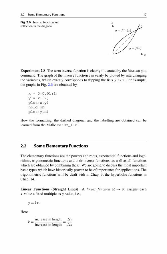
2.2 Some Elementary Functions 17
Fig. 2.6 Inverse function andreflection in the diagonal
Experiment 2.8 The term inverse function is clearly illustrated by the MATLAB plotcommand. The graph of the inverse function can easily be plotted by interchangingthe variables, which exactly corresponds to flipping the lists y ↔ x. For example,the graphs in Fig. 2.6 are obtained by
x = 0:0.01:1;y = x.ˆ2;plot(x,y)hold onplot(y,x)
How the formatting, the dashed diagonal and the labelling are obtained can belearned from the M-file mat02_1.m.
2.2 Some Elementary Functions
The elementary functions are the powers and roots, exponential functions and loga-rithms, trigonometric functions and their inverse functions, as well as all functionswhich are obtained by combining these. We are going to discuss the most importantbasic types which have historically proven to be of importance for applications. Thetrigonometric functions will be dealt with in Chap. 3, the hyperbolic functions inChap. 14.
Linear Functions (Straight Lines) A linear function R → R assigns eachx-value a fixed multiple as y-value, i.e.,
y = kx.
Here
k = increase in height
increase in length= �y
�x

18 2 Real-Valued Functions
Fig. 2.7 Equation of a straight line
is the slope of the graph, which is a straight line through the origin. The connectionbetween the slope and the angle between the straight line and x-axis is discussed inSect. 3.1. Adding an intercept d ∈ R translates the straight line d units in y-direction(Fig. 2.7). The equation is then
y = kx + d.
Quadratic Parabolas The quadratic function with domain D = R in its basicform is given by
y = x2.
Compression/stretching, horizontal and vertical translation are obtained via
y = αx2, y = (x − β)2, y = x2 + γ.
The effect of these transformations on the graph can be seen in Fig. 2.8.
α > 1 . . . compression in x-direction
0 < α < 1 . . . stretching in x-direction
α < 0 . . . reflection in the x-axis
β > 0 . . . translation to the right γ > 0 . . . translation upwards
β < 0 . . . translation to the left γ < 0 . . . translation downwards
The general quadratic function can be reduced to these cases by completing thesquare:
y = ax2 + bx + c
= a
(x + b
2a
)2
+ c − b2
4a
= α(x − β)2 + γ.

2.2 Some Elementary Functions 19
Fig. 2.8 Quadratic parabolas
Power Functions In the case of an integer exponent n ∈ N the following rulesapply:
xn = x · x · x · · · · · x (n factors), x1 = x,
x0 = 1, x−n = 1
xn(x �= 0).
The behaviour of y = x3 can be seen in the picture on the right-hand side ofFig. 2.3, the one of y = x4 in the picture on the left-hand side of Fig. 2.4. Thegraphs for odd and even powers behave similarly.
Experiment 2.9 On the website of maths online go to Functions 1 in the galleryarea and experiment with the applets Graphs of simple power functions and Cubicpolynomials and familiarise yourself with the Function plotter.
As an example of fractional exponents we consider the root functions y = n√
x =x1/n for n ∈ N with domain D = [0,∞). Here y = n
√x is defined as the inverse
function of the nth power; see Fig. 2.9 left. The graph of y = x−1 with domainD = R \ {0} is pictured in Fig. 2.9 right.
Absolute Value, Sign and Indicator Function The graph of the absolute valuefunction
y = |x| ={
x, x ≥ 0,
−x, x < 0
has a kink at the point (0,0); see Fig. 2.10 left.

20 2 Real-Valued Functions
Fig. 2.9 Power functions with fractional and negative exponents
Fig. 2.10 Absolute value and sign
The graph of the sign function or signum function
y = signx =
⎧⎪⎨⎪⎩
1, x > 0,
0, x = 0,
−1, x < 0
has a jump at x = 0 (Fig. 2.10 right). The indicator function of a subset A ⊂ R isdefined as
1A(x) ={
1, x ∈ A,
0, x /∈ A.
Exponential Functions and Logarithms Integer powers of a number a > 0 havejust been defined. Fractional (rational) powers give
a1/n = n√
a, am/n = ( n√
a)m = n√
am.
If r is an arbitrary real number, then ar is defined by its approximations am/n, wheremn
is the rational approximation to r obtained by decimal expansion.

2.2 Some Elementary Functions 21
Fig. 2.11 Exponential functions
Example 2.10 2π is defined by the sequence
23, 23.1, 23.14, 23.141, 23.1415, . . . ,
where
23.1 = 231/10 = 10√
231; 23.14 = 2314/100 = 100√
2314; . . . etc.
This somewhat informal introduction of the exponential function should be suffi-cient to have some examples at hand for applications in the following sections. Withthe tools we have developed so far we cannot yet show that this process of approx-imation actually leads to a well-defined mathematical object. The success of thisprocess is based on the completeness of the real numbers. This will be thoroughlydiscussed in Chap. 5.
From the definition above we obtain the following rules of calculation, valid forrational exponents:
aras = ar+s ,(ar
)s = ars = (as
)r,
arbr = (ab)r
for a, b > 0 and arbitrary r, s ∈ Q. The fact that these rules are also true for real-valued exponents r, s ∈ R can be shown by employing a limiting argument.
The graph of the exponential function with base a, the function y = ax , increasesfor a > 1 and decreases for a < 1; see Fig. 2.11. Its proper range is B = (0,∞);the exponential function is bijective from R to (0,∞). Its inverse function is thelogarithm to the base a (with domain (0,∞) and range R):
y = ax ⇔ x = loga y.
For example, log10 2 is the power by which 10 needs to be raised to obtain 2:
2 = 10log10 2.

22 2 Real-Valued Functions
Other examples are, for instance,
2 = log10(102), log10 10 = 1, log10 1 = 0, log10 0.001 = −3.
Euler’s number1 e is defined by
e = 1 + 1
1+ 1
2+ 1
6+ 1
24+ · · ·
= 1 + 1
1! + 1
2! + 1
3! + 1
4! + · · · =∞∑
j=0
1
j !≈ 2.718281828459045235360287471 . . . .
That this summation of infinitely many numbers can be defined rigorously will beproven in Chap. 5 by invoking the completeness of the real numbers. The logarithmto the base e is called natural logarithm and is denoted by log:
logx = loge x.
In some books the natural logarithm is denoted by lnx. We stick to the notationlogx, which is used, e.g., in MATLAB. The following rules are obtained directly byrewriting the rules for the exponential function:
u = elogu,
log(uv) = logu + logv,
log(uz
) = z logu,
for u,v > 0 and arbitrary z ∈ R. In addition, the following holds:
u = log(eu
),
for all u ∈ R, and log e = 1. In particular it follows from the above that
log1
u= − logu, log
v
u= logv − logu.
The graphs of y = logx and y = log10 x are shown in Fig. 2.12.
2.3 Exercises
1. How does the graph of an arbitrary function y = f (x) : R → R change underthe transformations
y = f (ax), y = f (x − b), y = cf (x), y = f (x) + d,
1L. Euler, 1707–1783.

2.3 Exercises 23
Fig. 2.12 Logarithms to thebase e and to the base 10
with a, b, c, d ∈ R? Distinguish the following different cases for a:
a < −1, −1 ≤ a < 0, 0 < a ≤ 1, a > 1,
and for b, c, d the cases
b, c, d > 0, b, c, d < 0.
Sketch the resulting graphs.2. Let the function f : D → R : x �→ 3x4 −2x3 −3x2 +1 be given. Using MATLAB
plot the graphs of f for
D = [−1,1.5], D = [−0.5,0.5], D = [0.5,1.5].Explain the behaviour of the function for D = R and find
f([−1,1.5]), f
((−0.5,0.5)
), f
((−∞,1]).
3. Which of the following functions are injective/surjective/bijective?
f : N → N : n �→ n2 − 6n + 10;g : R → R : x �→ |x + 1| − 3;h : R → R : x �→ x3.
Hint. Illustrative examples for the use of the MATLAB plot command may befound in the M-file mat02_2.m.
4. Check that the following functions D → B are bijective in the given regionsand compute the inverse function in each case:
y = −2x + 3, D = R, B = R;y = x2 + 1, D = (−∞,0], B = [1,∞);y = x2 − 2x − 1, D = [1,∞), B = [−2,∞).
24 2 Real-Valued Functions
5. On the website of maths online go to Functions 1 in the gallery area and solvethe exercises set in the applets Recognize functions 1 and Recognize graphs 1.Explain your results. Go to Interactive tests, Functions 1 and work on The bigfunction graph puzzle.
6. On the website of maths online go to Functions 2 in the gallery area and solvethe exercises set in the applets Recognize functions 2 and Recognize graphs 2.Explain your results.
7. Find the equation of the straight line through the points (1,1) and (4,3) as wellas the equation of the quadratic parabola through the points (−1,6), (0,5) and(2,21).
8. Let the amount of a radioactive substance at time t = 0 be A grams. Accordingto the law of radioactive decay, there remain A · qt grams after t days. Computeq for radioactive iodine 131 from its half life (8 days) and work out after howmany days 1
100 of the original amount of iodine 131 is remaining.Hint. The half life is the time span after which only half of the initial amount ofradioactive substance is remaining.
9. Let I [W/cm2] be the sound intensity of a sound wave that hits a detector sur-face. According to the Weber–Fechner law, its sound level L [Phon] is com-puted by
L = 10 log10(I/I0)
where I0 = 10−16 W/cm2. If the intensity I of a loudspeaker produces a soundlevel of 80 Phon, which level is then produced by an intensity of 2I by twoloudspeakers?
10. For x ∈ R the floor function �x� denotes the largest integer not greater than x,i.e.,
�x� = max{n ∈ N; n ≤ x}.Plot the following functions with domain D = [0,10] using the MATLAB com-mand floor:
y = �x�, y = x − �x�, y = (x − �x�)3
, y = (�x�)3.
Try to program correct plots in which the vertical connecting lines do not ap-pear.
11. Draw the graph of the function f : R → R : y = ax + signx for different valuesof a. Distinguish between the cases a > 0, a = 0, a < 0. For which values of a
is the function f injective and surjective, respectively?12. A function f : D = {1,2, . . . ,N} → B = {1,2, . . . ,N} is given by the list of its
function values y = (y1, . . . , yN), yi = f (i). Write a MATLAB program whichdetermines whether f is bijective. Test your program by generating randomy-values using
(a) y = unirnd(N,1,N), (b) y = randperm(N).
Hint. See the two M-files mat02_ex12a.m and mat02_ex12b.m.
3Trigonometry
Trigonometric functions play a major role in geometric considerations as well as inthe modelling of oscillations. We introduce these functions at the right-angled tri-angle and extend them periodically to R using the unit circle. Furthermore, we willdiscuss the inverse functions of the trigonometric functions in this chapter. As anapplication we will consider the transformation between Cartesian and polar coor-dinates.
3.1 Trigonometric Functions at the Triangle
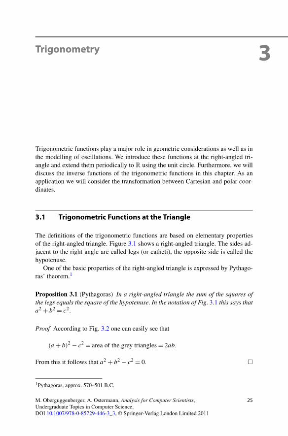
The definitions of the trigonometric functions are based on elementary propertiesof the right-angled triangle. Figure 3.1 shows a right-angled triangle. The sides ad-jacent to the right angle are called legs (or catheti), the opposite side is called thehypotenuse.
One of the basic properties of the right-angled triangle is expressed by Pythago-ras’ theorem.1
Proposition 3.1 (Pythagoras) In a right-angled triangle the sum of the squares ofthe legs equals the square of the hypotenuse. In the notation of Fig. 3.1 this says thata2 + b2 = c2.
Proof According to Fig. 3.2 one can easily see that
(a + b)2 − c2 = area of the grey triangles = 2ab.
From this it follows that a2 + b2 − c2 = 0. �
1Pythagoras, approx. 570–501 B.C.
M. Oberguggenberger, A. Ostermann, Analysis for Computer Scientists,Undergraduate Topics in Computer Science,DOI 10.1007/978-0-85729-446-3_3, © Springer-Verlag London Limited 2011
25

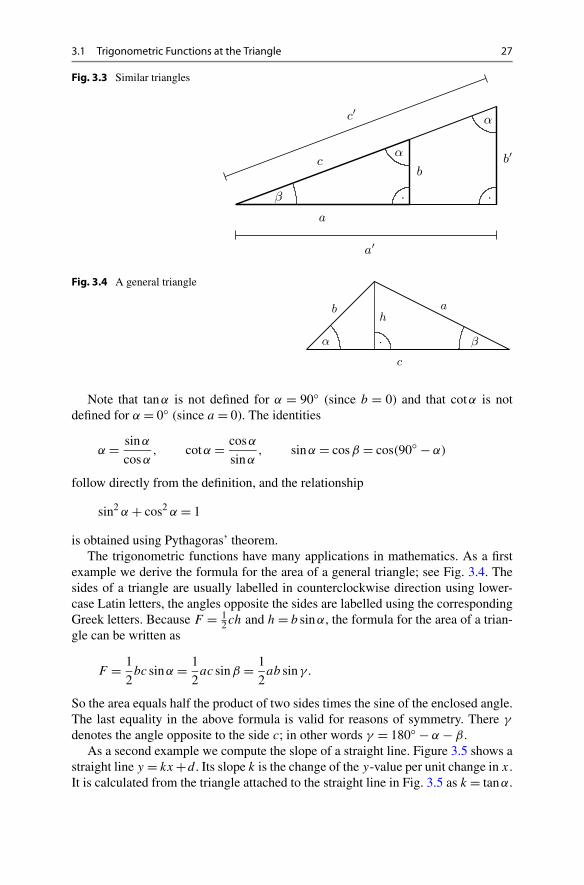
3.1 Trigonometric Functions at the Triangle 27
Fig. 3.3 Similar triangles
Fig. 3.4 A general triangle
Note that tanα is not defined for α = 90◦ (since b = 0) and that cotα is notdefined for α = 0◦ (since a = 0). The identities
α = sinα
cosα, cotα = cosα
sinα, sinα = cosβ = cos(90◦ − α)
follow directly from the definition, and the relationship
sin2 α + cos2 α = 1
is obtained using Pythagoras’ theorem.The trigonometric functions have many applications in mathematics. As a first
example we derive the formula for the area of a general triangle; see Fig. 3.4. Thesides of a triangle are usually labelled in counterclockwise direction using lower-case Latin letters, the angles opposite the sides are labelled using the correspondingGreek letters. Because F = 1
2ch and h = b sinα, the formula for the area of a trian-gle can be written as
F = 1
2bc sinα = 1
2ac sinβ = 1
2ab sinγ.
So the area equals half the product of two sides times the sine of the enclosed angle.The last equality in the above formula is valid for reasons of symmetry. There γ
denotes the angle opposite to the side c; in other words γ = 180◦ − α − β .As a second example we compute the slope of a straight line. Figure 3.5 shows a
straight line y = kx +d . Its slope k is the change of the y-value per unit change in x.It is calculated from the triangle attached to the straight line in Fig. 3.5 as k = tanα.

28 3 Trigonometry
Fig. 3.5 Straight line withslope k
Fig. 3.6 Relationshipbetween degrees and radianmeasure
In order to have simple formulas such as
d
dxsinx = cosx,
one has to measure the angle in radian measure. The connection between degreeand radian measure can be seen from the unit circle (the circle with centre 0 andradius 1); see Fig. 3.6.
The radian measure of the angle α (in degrees) is defined as the length � of thecorresponding arc of the unit circle with the sign of α. The arc length � on the unitcircle has no physical unit. However, one speaks of radians (rad) to emphasise thedifference to degrees.
As is generally known, the circumference of the unit circle is 2π with the con-stant
π = 3.141592653589793 . . . ≈ 22
7.
For the conversion between the two measures we use that 360◦ corresponds to 2π
in radian measure, for short 360◦ ↔ 2π [rad], so
α◦ ↔ π
180α [rad] and � [rad] ↔
(180
π�
)◦,
respectively. For example, 90◦ ↔ π2 and −270◦ ↔ − 3π
2 . Henceforth, we alwaysmeasure angles in radians.

3.2 Extension of the Trigonometric Functions to R 29
Fig. 3.7 Definition of thetrigonometric functions onthe unit circle
Fig. 3.8 Extension of thetrigonometric functions onthe unit circle
3.2 Extension of the Trigonometric Functions to R
For 0 ≤ α ≤ π2 the values sinα, cosα, tanα and cotα have a simple interpretation
on the unit circle; see Fig. 3.7. This representation follows from the fact that thehypotenuse of the defining triangle has length 1 on the unit circle.
One now extends the definition of the trigonometric functions for 0 ≤ α ≤ 2π bycontinuation with the help of the unit circle. A general point P on the unit circle,which is defined by the angle α, is assigned the coordinates
P = (cosα, sinα);
see Fig. 3.8. For 0 ≤ α ≤ π2 this is compatible with the earlier definition. For larger
angles the sine and cosine functions are extended to the interval [0,2π] by thisconvention. For example, it follows from the above that
sinα = − sin(α − π), cosα = − cos(α − π)
for π ≤ α ≤ 3π2 ; see Fig. 3.8.
For arbitrary values α ∈ R one finally defines sinα and cosα by periodic contin-uation with period 2π . For this purpose one first writes α = x + 2kπ with a uniquex ∈ [0,2π) and k ∈ Z. Then one sets
sinα = sin(x + 2kπ) = sinx, cosα = cos(x + 2kπ) = cosx.

30 3 Trigonometry
Fig. 3.9 The graphs of the sine and cosine functions in the interval [−2π,2π]
With the help of the formulae
tanα = sinα
cosα, cotα = cosα
sinα
the tangent and cotangent functions are extended as well. Since the sine functionequals zero for integer multiples of π , the cotangent is not defined for such argu-ments. Likewise the tangent is not defined for odd multiples of π
2 .The graphs of the functions y = sinx, y = cosx are shown in Fig. 3.9. The do-
main of both functions is D = R.The graphs of the functions y = tanx and y = cotx are presented in Fig. 3.10.
The domain D for the tangent is, as explained above, given by D = {x ∈ R; x �=π2 + kπ, k ∈ Z}, the one for the cotangent is D = {x ∈ R; x �= kπ, k ∈ Z}.
Many relations are valid between the trigonometric functions. For example, thefollowing addition theorems, which can be proven by elementary geometrical con-siderations, are valid; see Exercise 2. The maple commands expand and com-bine use such identities to simplify trigonometric expressions.
Proposition 3.3 (Addition theorems) For x, y ∈ R the following holds:
sin(x + y) = sinx cosy + cosx siny,
cos(x + y) = cosx cosy − sinx siny.

3.3 Cyclometric Functions 31
Fig. 3.10 The graphs of the tangent (left) and cotangent (right) functions
A wealth of material on trigonometric functions can be found on the website ofmaths online. We refer to the gallery, where one can find, under the link Trigono-metric Functions, the applet Definition of the trig functions and under Functions 2the applet The graphs of sin, cos and tan.
3.3 Cyclometric Functions
The cyclometric functions are inverse to the trigonometric functions in the appro-priate bijectivity regions.
Sine and Arcsine The sine function is bijective from the interval [−π2 , π
2 ] to therange [−1,1]; see Fig. 3.9. This part of the graph is called the principal branch ofthe sine. Its inverse function is called the arcsine (or sometimes inverse sine); seeFig. 3.11:
arcsin : [−1,1] →[−π
2,π
2
].
According to the definition of the inverse function it follows that
sin(arcsiny) = y for all y ∈ [−1,1].However, the converse formula is only valid for the principal branch, i.e.,
arcsin(sinx) = x is only valid for − π
2≤ x ≤ π
2.
For example, arcsin(sin 4) = −0.8584073 . . . �= 4.

32 3 Trigonometry
Fig. 3.11 The principal branch of the sine (left); the arcsine function (right)
Fig. 3.12 The principal branch of the cosine (left); the arccosine function (right)
Cosine and Arccosine Likewise, the principal branch of the cosine is defined asthe restriction of the cosine to the interval [0,π] with range [−1,1]. The principalbranch is bijective, and its inverse function is called the arccosine (or sometimesinverse cosine); see Fig. 3.12:
arccos : [−1,1] → [0,π].
Tangent and Arctangent As can be seen in Fig. 3.10 the restriction of the tangentto the interval (−π
2 , π2 ) is bijective. Its inverse function is called the arctangent (or
inverse tangent); see Fig. 3.13:
arctan : R →(
−π
2,π
2
).
To be precise, this is again the principal branch of the inverse tangent.
Application 3.4 (Polar coordinates in the plane) The polar coordinates (r, ϕ) of apoint P = (x, y) in the plane are obtained by prescribing its distance r from the

3.3 Cyclometric Functions 33
Fig. 3.13 The principal branch of the arctangent
Fig. 3.14 Plane polarcoordinates
origin and the angle ϕ with the positive x-axis (in counterclockwise direction); seeFig. 3.14.
The connection between Cartesian and polar coordinates is therefore describedby
x = r cosϕ,
y = r sinϕ,
where 0 ≤ ϕ < 2π and r ≥ 0. The range −π < ϕ ≤ π is also often used.In the converse direction the following conversion formulae are valid:
r =√
x2 + y2,
ϕ = arctany
x(in the region x > 0; −π
2 < ϕ < π2 ),
ϕ = signy · arccosx√
x2 + y2(if y �= 0 or x > 0; −π < ϕ < π).
The reader is encouraged to verify these formulas with the help of maple.


4Complex Numbers
Complex numbers are not just useful when solving polynomial equations, but theyplay an important role in many fields of mathematical analysis. With the help ofcomplex functions, transformations of the plane can be expressed, solution formulaefor differential equations can be obtained, and matrices can be classified. Not least,fractals can be defined by complex iteration processes. In this section we introducecomplex numbers and then discuss some elementary complex functions, like thecomplex exponential function. Applications can be found in Chaps. 9 (fractals), 20(systems of differential equations) and in Appendix B (normal form of matrices).
4.1 The Notion of Complex Numbers
The set of complex numbers C represents an extension of the real numbers in whichthe polynomial z2 +1 has a root. Complex numbers can be introduced as pairs (a, b)
of real numbers for which addition and multiplication is defined as follows:
(a, b) + (c, d) = (a + c, b + d),
(a, b) · (c, d) = (ac − bd, ad + bc).
The real numbers are considered as the subset of all pairs of the form (a,0), a ∈ R.Squaring the pair (0,1) shows that
(0,1) · (0,1) = (−1,0).
The square of (0,1) thus corresponds to the real number −1. Therefore, (0,1) pro-vides a root for the polynomial z2 + 1. This root is denoted by i; in other words
i2 = −1.
Using this notation and rewriting the pairs (a, b) in the form a + ib, one obtains acomputationally more convenient representation of the set of complex numbers:
C = {a + ib; a ∈ R, b ∈ R}.M. Oberguggenberger, A. Ostermann, Analysis for Computer Scientists,Undergraduate Topics in Computer Science,DOI 10.1007/978-0-85729-446-3_4, © Springer-Verlag London Limited 2011
37

38 4 Complex Numbers
The rules of calculation with pairs (a, b) then simply amount to common calcula-tions with the expressions a + ib with the additional rule that i2 = −1:
(a + ib) + (c + id) = a + c + i(b + d),
(a + ib)(c + id) = ac + ibc + iad + i2bd
= ac − bd + i(ad + bc).
So, for example,
(2 + 3i)(−1 + i) = −5 − i.
Definition 4.1 For the complex number z = x + iy,
x = Re z, y = Im z
denote the real part and the imaginary part of z, respectively. The real number
|z| =√
x2 + y2
is the absolute value (or modulus) of z, and
z = x − iy
is the complex conjugate to z.
A simple calculation shows that
zz = (x + iy)(x − iy) = x2 + y2 = |z|2,which means that zz is always a real number. From this we obtain the rule for cal-culating with fractions:
u + iv
x + iy=
(u + iv
x + iy
)(x − iy
x − iy
)= (u + iv)(x − iy)
x2 + y2= ux + vy
x2 + y2+ i
vx − uy
x2 + y2.
It is achieved by expansion with the complex conjugate of the denominator. Appar-ently one can therefore divide by any complex number not equal to zero, and the setC forms a field.
Experiment 4.2 Type in MATLAB: z = complex(2,3) (equivalently, z =2+3*i or z = 2+3*j) as well as w = complex(-1,1) and try out the com-mands z * w, z/w as well as real(z), imag(z), conj(z), abs(z).
Clearly every negative real x has two square roots in C, namely i√|x| and
−i√|x|. Moreover, the fundamental theorem of algebra says that C is algebraically
closed. Thus every polynomial equation
αnzn + αn−1z
n−1 + · · · + α1z + α0 = 0

4.1 The Notion of Complex Numbers 39
Fig. 4.1 Complex plane
with coefficients αj ∈ C, αn �= 0 has n complex solutions (counted with their multi-plicity).
Example 4.3 (Taking the square root of complex numbers) The equation z2 = a+ ibcan be solved by the ansatz
(x + iy)2 = a + ib
so
x2 − y2 = a, 2xy = b.
If one uses the second equation to express y through x and substitutes this into thefirst equation, one obtains the quartic equation
x4 − ax2 − b2/4 = 0.
Solving this by the substitution t = x2 one obtains two real solutions. In the case ofb = 0, either x or y equals zero depending on the sign of a.
The Complex Plane A geometric representation of the complex numbers is ob-tained by identifying z = x + iy ∈ C with the point (x, y) ∈ R
2 in the coordinateplane (Fig. 4.1). Geometrically |z| = √
x2 + y2 is the distance of point (x, y) fromthe origin; the complex conjugate z = x − iy is obtained by reflection in the x-axis.
The polar representation of a complex number z = x + iy is obtained like inApplication 3.4 by
r = |z|, ϕ = arg z.
The angle ϕ to the positive x-axis is called argument of the complex number, where-upon the choice of the interval −π < ϕ ≤ π defines the principal value Arg z of theargument. Thus
z = x + iy = r(cosϕ + i sinϕ).
The multiplication of two complex numbers z = r(cosϕ + i sinϕ), w = s(cosψ +i sinψ) in polar representation corresponds to the product of the absolute values andthe sum of the angles:
zw = rs(
cos(ϕ + ψ) + i sin(ϕ + ψ)),

40 4 Complex Numbers
which follows from the addition formulae for sine and cosine:
sin(ϕ + ψ) = sinϕ cosψ + cosϕ sinψ,
cos(ϕ + ψ) = cosϕ cosψ − sinϕ sinψ;see Proposition 3.3.
4.2 The Complex Exponential Function
An important tool for the representation of complex numbers and functions, but alsofor the real trigonometric functions, is given by the complex exponential function.For z = x + iy this function is defined by
ez = ex(cosy + i siny).
The complex exponential function maps C to C \ {0}. We will study its mapping be-haviour below. It is an extension of the real exponential function, i.e., if z = x ∈ R,then ez = ex . This is in accordance with the previously defined real-valued expo-nential function. We also use the notation exp(z) for ez.
The addition theorems for sine and cosine imply the usual rules of calculation
ez+w = ezew, e0 = 1,(ez
)n = enz,
valid for z,w ∈ C and n ∈ Z. In contrast to the case when z is a real number, the lastrule (for raising to powers) is generally not true, if n is not an integer.
Exponential Function and Polar Coordinates According to the definition theexponential function of a purely imaginary number iϕ equals
eiϕ = cosϕ + i sinϕ,
∣∣eiϕ∣∣ =
√cos2 ϕ + sin2 ϕ = 1.
Thus the complex numbers{eiϕ; −π < ϕ ≤ π
}lie on the unit circle (Fig. 4.2).
For example, the following identities hold:
eiπ/2 = i, eiπ = −1, e2iπ = 1, e2kiπ = 1 (k ∈ Z).
Using r = |z|, ϕ = Arg z results in the especially simple form of the polar represen-tation
z = reiϕ.
Taking roots is accordingly simple.

4.3 Mapping Properties of Complex Functions 41
Fig. 4.2 The unit circle inthe complex plane
Example 4.4 (Taking square roots in complex polar coordinates) If z2 = reiϕ , thenone obtains the two solutions ±√
reiϕ/2 for z. For example, the problem
z2 = 2i = 2eiπ/2
has the two solutions
z = √2eiπ/4 = 1 + i
and
z = −√2eiπ/4 = −1 − i.
Euler’s Formulae By addition and subtraction, respectively, of the relations
eiϕ = cosϕ + i sinϕ,
e−iϕ = cosϕ − i sinϕ
one obtains at once Euler’s formulae
cosϕ = 1
2
(eiϕ + e−iϕ)
,
sinϕ = 1
2i
(eiϕ − e−iϕ)
.
They permit a representation of the real trigonometric functions by means of thecomplex exponential function.
4.3 Mapping Properties of Complex Functions
In this section we study the mapping properties of complex functions. More pre-cisely, we ask how their effect can be described geometrically. Let
f : D ⊂ C → C : z �→ w = f (z)
42 4 Complex Numbers
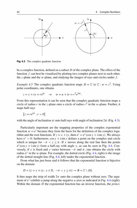
Fig. 4.3 The complex quadratic function
be a complex function, defined on a subset D of the complex plane. The effect of thefunction f can best be visualised by plotting two complex planes next to each other,the z-plane and the w-plane, and studying the images of rays and circles under f .
Example 4.5 The complex quadratic function maps D = C to C : w = z2. Usingpolar coordinates, one obtains
z = x + iy = reiϕ ⇒ w = u + iv = r2e2iϕ.
From this representation it can be seen that the complex quadratic function maps acircle of radius r in the z-plane onto a circle of radius r2 in the w-plane. Further, itmaps half-rays
{z = reiψ : r > 0
}with the angle of inclination ψ onto half-rays with angle of inclination 2ψ (Fig. 4.3).
Particularly important are the mapping properties of the complex exponentialfunction w = ez because they form the basis for the definition of the complex loga-rithm and the root functions. If z = x + iy, then ez = ex(cosy + i siny). We alwayshave ex > 0; furthermore, cosy + i siny defines a point on the complex unit circlewhich is unique for −π < y ≤ π . If x moves along the real line then the pointsex(cosy + i siny) form a half-ray with angle y, as can be seen in Fig. 4.4. Con-versely, if x is fixed and y varies between −π and π , one obtains the circle withradius ex in the w-plane. For example, the dotted circle (Fig. 4.4, right) is the imageof the dotted straight line (Fig. 4.4, left) under the exponential function.
From what has just been said it follows that the exponential function is bijectiveon the domain
D = {z = x + iy; x ∈ R, −π < y ≤ π} → B = C \ {0}.It thus maps the strip of width 2π onto the complex plane without zero. The argu-ment of ez exhibits a jump along the negative u-axis as indicated in Fig. 4.4 (right).Within the domain D the exponential function has an inverse function, the princi-


44 4 Complex Numbers
2. Rewrite the following complex numbers in the form z = reiϕ and sketch them inthe complex plane:
z = −1 − i, z = −5, z = 3i, z = 2 − 2i.
3. Compute the two complex solutions of the equation
z2 = 2 + 2i
with the help of the ansatz z = x + iy and equating the real and the imaginarypart. Test and explain the MATLAB-commands
roots([2,0,-2-2*i])sqrt(2+2*i).
4. Compute the two complex solutions of the equation
z2 = 2 + 2i
in the form z = reiϕ from the polar representation of 2 + 2i.5. Compute the four complex solutions of the quartic equation
z4 − 2z2 + 2 = 0
by hand and with MATLAB (command roots).6. Let z = x + iy, w = u + iv. Check the formula ez+w = ezew by using the defini-
tion and applying the addition theorems for the trigonometric functions.7. Compute z = Logw for
w = 1 + i, w = −5i, w = −1.
Sketch w and z in the complex plane and verify your results with the help of therelation w = ez and with MATLAB (command log).

5Sequences and Series
The concept of a limiting process at infinity is one of the central ideas of math-ematical analysis. It forms the basis for all its essential concepts, like continuity,differentiability, series expansions of functions, integration, etc. The transition fromthe discrete to the continuous constitutes the modelling strength of mathematicalanalysis. Discrete models of physical, technical or economic processes can often bebetter and easier understood, provided that the number of their atoms—their dis-crete building blocks—is sufficiently big, if they are approximated by a continuousmodel with the help of a limiting process. The transition from difference equationsfor biological growth processes in discrete time to differential equations in contin-uous time or the description of share prices by stochastic processes in continuoustime are examples for that. The majority of models in physics are field models, thatis, they are expressed in a continuous space and time structure. Even though themodels are discretised again in numerical approximations, the continuous model isstill helpful as a background, for example for the derivation of error estimates.
The following sections are dedicated to the specification of the idea of limitingprocesses. This chapter starts by studying infinite sequences and series, gives someapplications and covers the corresponding notion of a limit. One of the achieve-ments which we especially emphasise is the completeness of the real numbers. Itguarantees the existence of limits for arbitrary monotonically increasing boundedsequences of numbers, the existence of zeros of continuous functions, of maximaand minima of differentiable functions, of integrals etc. It is an indispensable build-ing block of mathematical analysis.
5.1 The Notion of an Infinite Sequence
Definition 5.1 Let X be a set. An (infinite) sequence with values in X is a mappingfrom N to X.
M. Oberguggenberger, A. Ostermann, Analysis for Computer Scientists,Undergraduate Topics in Computer Science,DOI 10.1007/978-0-85729-446-3_5, © Springer-Verlag London Limited 2011
45
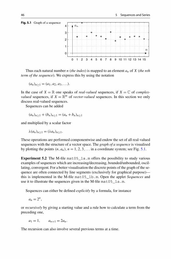
46 5 Sequences and Series
Fig. 5.1 Graph of a sequence
Thus each natural number n (the index) is mapped to an element an of X (the nthterm of the sequence). We express this by using the notation
(an)n≥1 = (a1, a2, a3, . . .).
In the case of X = R one speaks of real-valued sequences, if X = C of complex-valued sequences, if X = R
m of vector-valued sequences. In this section we onlydiscuss real-valued sequences.
Sequences can be added
(an)n≥1 + (bn)n≥1 = (an + bn)n≥1
and multiplied by a scalar factor
λ(an)n≥1 = (λan)n≥1.
These operations are performed componentwise and endow the set of all real-valuedsequences with the structure of a vector space. The graph of a sequence is visualisedby plotting the points (n, an), n = 1,2,3, . . . in a coordinate system; see Fig. 5.1.
Experiment 5.2 The M-file mat05_1a.m offers the possibility to study variousexamples of sequences which are increasing/decreasing, bounded/unbounded, oscil-lating, convergent. For a better visualisation the discrete points of the graph of the se-quence are often connected by line segments (exclusively for graphical purpose)—this is implemented in the M-file mat05_1b.m. Open the applet Sequences anduse it to illustrate the sequences given in the M-file mat05_1a.m.
Sequences can either be defined explicitly by a formula, for instance
an = 2n,
or recursively by giving a starting value and a rule how to calculate a term from thepreceding one,
a1 = 1, an+1 = 2an.
The recursion can also involve several previous terms at a time.
5.1 The Notion of an Infinite Sequence 47
Example 5.3 A discrete population model which goes back to Verhulst1 (limitedgrowth) describes the population xn at the point in time n (time intervals of length 1)by the recursive relation
xn+1 = xn + βxn(L − xn).
Here β is a growth factor and L the limiting population, i.e., the population whichis not exceeded in the long-term (short-term overruns are possible, however, leadto immediate decay of the population). Additionally one has to prescribe the initialpopulation x1 = A. According to the model the population increase xn+1 −xn duringone time interval is proportional to the existing population and to the difference tothe population limit. The M-file mat05_2.m contains a MATLAB function, called
x = mat05_2(A,beta,N),
which computes and plots the first N terms of the sequence x = (x1, . . . , xN). Theinitial value is A, the growth rate β; L was set to L = 1. Experiments with A = 0.1,N = 50 and β = 0.5, β = 1, β = 2, β = 2.5, β = 3 show convergent, oscillating andchaotic behaviour of the sequence, respectively.
Below we develop some concepts which help to describe the behaviour of se-quences.
Definition 5.4 A sequence (an)n≥1 is called monotonically increasing, if
n ≤ m ⇒ an ≤ am;(an)n≥1 is called monotonically decreasing, if
n ≤ m ⇒ an ≥ am;(an)n≥1 is called bounded from above, if
∃T ∈ R ∀n ∈ N : an ≤ T .
We will show in Proposition 5.13 below that the set of upper bounds of a boundedsequence has a smallest element. This least upper bound T0 is called the supremumof the sequence and it is denoted by
T0 = supn∈N
an.
The supremum is characterised by the following two conditions:(a) an ≤ T0 for all n ∈ N;(b) if T is a real number and an ≤ T for all n ∈ N, then T ≥ T0.
1P.-F. Verhulst, 1804–1849.

48 5 Sequences and Series
Fig. 5.2 Convergence of asequence
Note that the supremum itself does not have to be a term of the sequence. However,if this is the case, it is called maximum of the sequence and denoted by
T0 = maxn∈N
an.
A sequence has a maximum T0 if the following two conditions are fulfilled:(a) an ≤ T0 for all n ∈ N;(b) there exists at least one m ∈ N such that am = T0.In the same way, a sequence (an)n≥1 is called bounded from below, if
∃S ∈ R ∀n ∈ N : S ≤ an.
The greatest lower bound is called infimum (or minimum, if it is attained by a termof the sequence).
Experiment 5.5 Investigate the sequences produced by the M-file mat05_1a.mwith regard to the concepts developed above.
As mentioned in the introduction to this chapter, the concept of convergence is acentral concept of mathematical analysis. Intuitively, it states that the terms of thesequence (an)n≥1 approach a limit a with growing index n. For example, in Fig. 5.2with a = 0.8 one has
|a − an| < 0.2 from n = 6, |a − an| < 0.05 from n = 21.
For a precise definition of the concept of convergence we first introduce the no-tion of an ε-neighbourhood of a point a ∈ R (ε > 0):
Uε(a) = {x ∈ R; |a − x| < ε
} = (a − ε, a + ε).
We say that a sequence (an)n≥1 settles in a neighbourhood Uε(a), if from a certainindex n(ε) on all subsequent terms an of the sequence lie in Uε(a).
Definition 5.6 The sequence (an)n≥1 converges to a limit a if it settles in eachε-neighbourhood of a.

5.1 The Notion of an Infinite Sequence 49
These facts can be expressed in quantifier notation as follows:
∀ε > 0 ∃n(ε) ∈ N ∀n ≥ n(ε) : |a − an| < ε.
If a sequence (an)n≥1 converges to a limit a, one writes
a = limn→∞an or an → a as n → ∞.
In the example of Fig. 5.2 the limit a is indicated as a dotted line, the neighbourhoodU0.2(a) as a strip with a dashed boundary line and the neighbourhood U0.05(a) as astrip with a solid boundary line.
In the case of convergence the limit can be interchanged with addition, multipli-cation and division (with the exception of zero), as expected.
Proposition 5.7 (Rules of calculation for limits) If the sequences (an)n≥1 and(bn)n≥1 are convergent then the following rules hold:
limn→∞(an + bn) = lim
n→∞an + limn→∞bn
limn→∞(λan) = λ lim
n→∞an (for λ ∈ R)
limn→∞(anbn) =
(lim
n→∞an
)(lim
n→∞bn
)
limn→∞(an/bn) =
(lim
n→∞an
)/(lim
n→∞bn
)(if lim
n→∞bn = 0)
Proof The verification of these trivialities is left to the reader as an exercise. Theproofs are not deep, but one has to carefully pick the right approach in order toverify the conditions of Definition 5.6. In order to illustrate at least once how suchproofs are done, we will show the statement about multiplication. Assume that
limn→∞an = a and lim
n→∞bn = b.
Let ε > 0. According to Definition 5.6 we have to find an index n(ε) ∈ N satisfying
|ab − anbn| < ε (5.1)
for all n ≥ n(ε). Due to the convergence of the sequence (an)n≥1 we can first findan n1(ε) ∈ N so that |a − an| ≤ 1 for all n ≥ n1(ε). For these n also
|an| = |an − a + a| ≤ 1 + |a|
applies. Furthermore, we can find n2(ε) ∈ N and n3(ε) ∈ N which guarantee that
|a − an| < ε
2 max(|b|,1)and |b − bn| < ε
2(1 + |a|)

50 5 Sequences and Series
for all n ≥ n2(ε) and n ≥ n3(ε), respectively. It thus follows that
|ab − anbn| = ∣∣(a − an)b + an(b − bn)∣∣ ≤ |a − an||b| + |an||b − bn|
≤ |a − an||b| + (|a| + 1)|b − bn| ≤ ε
2+ ε
2≤ ε
for all n ≥ n(ε) with n(ε) = max(n1(ε), n2(ε), n3(ε)). This is the statement that wasto be proven. �
The important ideas of the proof were: Splitting in two summands with the helpof the triangle inequality (see Exercise 2 of Chap. 1); bounding |an| by 1 + |a|using the assumed convergence; upper bounds for the terms |a − an| and |b − bn|by fractions of ε (again possible due to the convergence) so that the summandstogether stay less than ε. All elementary proofs of convergence in mathematicalanalysis proceed in a similar way.
Real-valued sequences with terms that increase to infinity with growing index n
have no limit in the sense of the definition given above. However, it is practical toassign them the symbol ∞ as an improper limit.
Definition 5.8 A sequence (an)n≥1 has the improper limit ∞ if it has the propertyof unlimited increase
∀T ∈ R ∃n(T ) ∈ N ∀n ≥ n(T ) : an ≥ T .
In this case, one writes
limn→∞an = ∞.
In the same way one defines
limn→∞bn = −∞, if lim
n→∞(−bn) = ∞.
Example 5.9 We consider the geometric sequence (qn)n≥1. Obviously the followingholds:
limn→∞qn = 0, if |q| < 1,
limn→∞qn = ∞, if q > 1,
limn→∞qn = 1, if q = 1.
For q ≤ −1 the sequence has no limit (neither proper nor improper).

5.2 The Completeness of the Set of Real Numbers 51
5.2 The Completeness of the Set of Real Numbers
As remarked in the introduction to this chapter, the completeness of the set of realnumbers is one of the pillars of real analysis. The property of completeness can beexpressed in different ways. We will use a simple formulation which is particularlyhelpful in many applications.
Proposition 5.10 (Completeness of the set of real numbers) Each monotonicallyincreasing sequence of real numbers that is bounded from above has a limit (in R).
Proof Let (an)n≥1 be a monotonically increasing, bounded sequence. First we provethe theorem in the case that all terms an are non-negative. We write the terms asdecimal numbers
an = A(n).α(n)1 α
(n)2 α
(n)3 . . . .
with A(n) ∈ N0, α(n)j ∈ {0,1, . . . ,9}. By assumption there is a bound T ≥ 0 so that
an ≤ T for all n. Therefore, also A(n) ≤ T for all n. But the sequence (A(n))n≥1is a monotonically increasing, bounded sequence of integers and therefore musteventually reach its least upper bound A (and stay there). In other words, thereexists n0 ∈ N such that
A(n) = A for all n ≥ n0.
Thus we have found the integer part of the limit a to be constructed:
a = A. . . . .
Let now α1 ∈ {0, . . . ,9} be the least upper bound for α(n)1 . As the sequence is mono-
tonically increasing there is again an n1 ∈ N with
α(n)1 = α1 for all n ≥ n1
and consequently
a = A.α1 . . . .
Let now α2 ∈ {0, . . . ,9} be the least upper bound for α(n)2 . There is an n2 ∈ N with
α(n)2 = α2 for all n ≥ n2
and consequently
a = A.α1α2 . . . .
Successively one defines a real number
a = A.α1α2α3α4 . . .

52 5 Sequences and Series
in that way. It remains to show that a = limn→∞ an. Let ε > 0. We first choosej ∈ N so that 10−j < ε. For n ≥ nj
a − an = 0.000 . . .0α(n)j+1α
(n)j+2 . . . ,
since the first j digits after the decimal point in a coincide with those of an providedn ≥ nj . Therefore,
|a − an| ≤ 10−j < ε for n ≥ nj .
With n(ε) = nj the condition required in Definition 5.6 is fulfilled.If the sequence (an)n≥1 also has negative terms, it can be transformed to a
sequence with non-negative terms by adding the absolute value of the first termwhich results in the sequence (|a1| + an)n≥1. Using the obvious rule lim(c + an) =c + liman allows to apply the first part of the proof. �
Remark 5.11 The set of rational numbers is not complete. For example, the decimalexpansion of
√2,
(1,1.4,1.41,1.414,1.4142, . . .)
is a monotonically increasing, bounded sequence of rational numbers (an upperbound is for example T = 1.5, since 1.52 > 2), but the limit
√2 does not belong
to Q (as it is an irrational number).
Example 5.12 (Arithmetic of real numbers) Due to Proposition 5.10 the arithmeti-cal operations on the real numbers introduced in Sect. 1.2 can be legitimised a pos-teriori. Let us look for instance at the addition of two non-negative real numbersa = A.α1α2 . . . and b = B.β1β2 . . . with A,B ∈ N0, αj ,βj ∈ {0,1, . . . ,9}. By trun-cating them after the nth decimal place we obtain two approximating sequences ofrational numbers an = A.α1α2 . . . αn and bn = B.β1β2 . . . βn with
a = limn→∞an, b = lim
n→∞bn.
The sum of two approximations an + bn is defined by the addition of rational num-bers in an elementary way. The sequence (an + bn)n≥1 is evidently monotonicallyincreasing and bounded from above, for instance by A+B +2. According to Propo-sition 5.10 this sequence has a limit and this limit defines the sum of the real numbers
a + b = limn→∞(an + bn).
In this way the addition of real numbers is rigorously justified. In a similar way onecan proceed with multiplication. Finally, Proposition 5.7 allows one to prove theusual rules for addition and multiplication.

5.3 Infinite Series 53
Consider a sequence with upper bound T . Each real number T1 > T is also anupper bound. We can now show that there always exists a smallest upper bound.A bounded sequence thus actually has a supremum as claimed earlier.
Proposition 5.13 Each sequence (an)n≥1 of real numbers which is bounded fromabove has a supremum.
Proof Let Tn = max{a1, . . . , an} be the maximum of the first n terms of the se-quence. These maxima on their part define a sequence (Tn)n≥1 which is boundedfrom above by the same bounds as (an)n≥1 but is additionally monotonically in-creasing. According to the previous proposition it has a limit T0. We are going toshow that this limit is the supremum of the original sequence. Indeed, as Tn ≤ T0for all n, we have an ≤ T0 for all n as well. Assume that the sequence (an)n≥1 hada smaller upper bound T < T0, i.e., an ≤ T for all n. This in turn implies Tn ≤ T
for all n and contradicts the fact that T0 = limTn. Therefore, T0 is the least upperbound. �
Application 5.14 We are now in a position to show that the construction of theexponential function for real exponents given informally in Sect. 2.2 is justified.Let a > 0 be a basis for the power ar to be defined with real exponent r ∈ R. Itis sufficient to treat the case r > 0 (for negative r , the expression ar is definedby the reciprocal of a|r|). We write r as the limit of a monotonically increasingsequence (rn)n≥1 of rational numbers by choosing for rn the decimal representationof r , truncated at the nth digit. The rules of calculation for rational exponents implythe inequality arn+1 − arn = arn(arn+1−rn − 1) ≥ 0. This shows that the sequence(arn)n≥1 is monotonically increasing. It is also bounded from above, for instanceby aq , if q is a rational number bigger than r . According to Proposition 5.10 thissequence has a limit. It defines ar .
Application 5.15 Let a > 0. Then limn→∞ n√
a = 1.In the proof we can restrict ourselves to the case 0 < a < 1 since otherwise theargument can be used for 1/a. One can easily see that the sequence ( n
√a )n≥1 is
monotonically increasing; it is also bounded from above by 1. Therefore, it has alimit b. Suppose that b < 1. From n
√a ≤ b we infer that a ≤ bn → 0 for n → ∞,
which contradicts the assumption a > 0. Consequently b = 1.
5.3 Infinite Series
Sums of the form
∞∑k=1
ak = a1 + a2 + a3 + · · ·

54 5 Sequences and Series
with infinitely many summands can be given a meaning under certain conditions.The starting point of our considerations is a sequence of coefficients (ak)k≥1 of realnumbers. The nth partial sum is defined as
Sn =n∑
k=1
ak = a1 + a2 + · · · + an,
thus
S1 = a1,
S2 = a1 + a2,
S3 = a1 + a2 + a3, etc.
As needed we also use the notation Sn = ∑nk=0 ak without further comment if the
sequence a0, a1, a2, a3, . . . starts with the index k = 0.
Definition 5.16 The sequence of the partial sums (Sn)n≥1 is called a series. If thelimit S = limn→∞ Sn exists, then the series is called convergent, otherwise diver-gent.
In the case of convergence one writes
S =∞∑
k=1
ak = limn→∞
(n∑
k=1
ak
).
In this way the summation problem is reduced to the question of convergence of thesequence of the partial sums.
Experiment 5.17 The M-file mat05_3.m, when called as mat05_3(N,Z), gen-erates the first N partial sums with time delay Z [seconds] of five series, i.e., itcomputes Sn for 1 ≤ n ≤ N in each case:
Series 1 : Sn =n∑
k=1
k−0.99, Series 2 : Sn =n∑
k=1
k−1,
Series 3 : Sn =n∑
k=1
k−1.01, Series 4 : Sn =n∑
k=1
k−2.
Series 5 : Sn =n∑
k=1
1
k! ,
Experiment with increasing values of N and try to see which series shows conver-gence or divergence.
5.3 Infinite Series 55
In the experiment the convergence of Series 5 seems obvious, while the observa-tions for the other series are rather not as conclusive. Actually, Series 1 and 2 aredivergent, while the others are convergent. This shows the need for analytical toolsin order to be able to decide the question of convergence. However, we first look ata few examples.
Example 5.18 (Geometric series) In this example we are concerned with the series∑∞k=0 qk with real factor q ∈ R. For the partial sums we deduce that
Sn =n∑
k=0
qk = 1 − qn+1
1 − q.
Indeed, by subtraction of the two lines
Sn = 1 + q + q2 + · · · + qn,
qSn = q + q2 + q3 + · · · + qn+1
one obtains the formula (1 − q)Sn = 1 − qn+1, from which the result follows.The case |q| < 1: As qn+1 → 0 the series converges with value
S = limn→∞
1 − qn+1
1 − q= 1
1 − q.
The case |q| > 1: For q > 1 the partial sum Sn = (qn+1 − 1)/
(q − 1) → ∞ and the series diverges. In the case of q < −1 the partial sumsSn = (1 − (−1)n+1|q|n+1)/(1 − q) are unbounded and oscillate. They thus divergeas well.
The case |q| = 1: For q = 1 we have Sn = 1 + 1 + · · · + 1 = n + 1 which tendsto infinity; for q = −1, the partial sums Sn oscillate between 1 and 0. In both casesthe series diverges.
Example 5.19 The nth partial sum of the series∑∞
k=11
k(k+1)is
Sn =n∑
k=1
1
k(k + 1)=
n∑k=1
(1
k− 1
k + 1
)
= 1 − 1
2+ 1
2− 1
3+ 1
3− 1
4+ · · · − 1
n+ 1
n− 1
n + 1= 1 − 1
n + 1.
It is called a telescopic sum. The series converges to
S =∞∑
k=1
1
k(k + 1)= lim
n→∞
(1 − 1
n + 1
)= 1.

56 5 Sequences and Series
Example 5.20 (Harmonic series) We consider the series∑∞
k=11k
. By combiningblocks of two, four, eight, sixteen, etc. elements, one obtains the grouping
1 + 1
2+
(1
3+ 1
4
)+
(1
5+ 1
6+ 1
7+ 1
8
)+
(1
9+ · · · + 1
16
)+
(1
17+ · · ·
)+ · · ·
≥ 1 + 1
2+
(1
4+ 1
4
)+
(1
8+ 1
8+ 1
8+ 1
8
)+
(1
16+ · · · + 1
16
)
+(
1
32+ · · ·
)+ · · ·
= 1 + 1
2+ 1
2+ 1
2+ 1
2+ 1
2+ · · · → ∞.
The partial sums tend to infinity, therefore, the series diverges.
There are a number of criteria which allow one to decide whether a series con-verges or diverges. Here we only discuss two simple comparison criteria, whichsuffice for our purposes. For further considerations we refer to the literature; forinstance [3, Chap. 9.2].
Proposition 5.21 (Comparison criteria) Let 0 ≤ ak ≤ bk for all k ∈ N or at leastfor all k greater than or equal to a certain k0. Then we have(a) If the series
∑∞k=1 bk is convergent then the series
∑∞k=1 ak converges, too.
(b) If the series∑∞
k=1 ak is divergent then the series∑∞
k=1 bk diverges, too.
Proof (a) The partial sums fulfil Sn = ∑nk=1 ak ≤ ∑∞
k=1 bk = T and Sn ≤ Sn+1,hence are bounded and monotonically increasing. According to Proposition 5.10the limit of the partial sums exists.
(b) This time, we have for the partial sums
Tn =n∑
k=1
bk ≥n∑
k=1
ak → ∞,
since the latter are positive and divergent. �
Under the condition 0 ≤ ak ≤ bk of the proposition one says that∑∞
k=1 bk domi-nates
∑∞k=1 ak . A series thus converges if it is dominated by a convergent series; it
diverges if it dominates a divergent series.
Example 5.22 The series∑∞
k=11k2 is convergent. For the proof we use that
n∑k=1
1
k2= 1 +
n−1∑j=1
1
(j + 1)2and aj = 1
(j + 1)2≤ 1
j (j + 1)= bj .
Example 5.19 shows that∑∞
j=1 bj converges. Proposition 5.21 then implies conver-gence of the original series.

5.4 Supplement: Accumulation Points of Sequences 57
Example 5.23 The series∑∞
k=1 k−0.99 diverges. This follows from the fact thatk−1 ≤ k−0.99. Therefore, the series
∑∞k=1 k−0.99 dominates the harmonic series
which itself is divergent; see Example 5.20.
Example 5.24 In Chap. 2 Euler’s number,
e =∞∑
j=0
1
j ! = 1 + 1 + 1
2+ 1
6+ 1
24+ 1
120+ · · · ,
was introduced. We can now show that this definition makes sense, i.e., the seriesconverges. For j ≥ 4 it is obvious that
j ! = 1 · 2 · 3 · 4 · 5 · . . . · j ≥ 2 · 2 · 2 · 2 · 2 · . . . · 2 = 2j .
Thus the geometric series∑∞
j=0
( 12
)j is a dominating convergent series.
Example 5.25 The decimal notation of a positive real number
a = A.α1α2α3 . . .
with A ∈ N0, αk ∈ {0, . . . ,9} can be understood as a representation by the series
a = A +∞∑
k=1
αk10−k.
The series converges since A + 9∑∞
k=1 10−k is a dominating convergent series.
5.4 Supplement: Accumulation Points of Sequences
Occasionally we need sequences which themselves do not converge but have con-vergent subsequences. The notions of accumulation points, limit superior and limitinferior are connected with this concept.
Definition 5.26 A number b is called accumulation point of a sequence (an)n≥1 ifeach neighbourhood Uε(b) of b contains infinitely many terms of the sequence:
∀ε > 0 ∀n ∈ N ∃m = m(n, ε) ≥ n : |b − am| < ε.
Figure 5.3 displays the sequence
an = arctann + cos(nπ/2) + 1
nsin(nπ/2).
It has three accumulation points, namely b1 = π/2 + 1 ≈ 2.57, b2 = π/2 ≈ 1.57and b3 = π/2 − 1 ≈ 0.57.
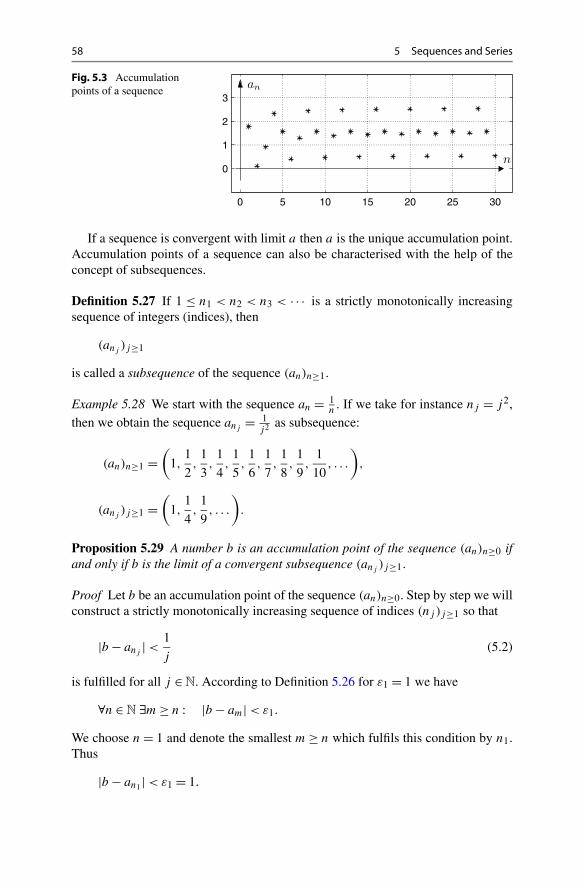
58 5 Sequences and Series
Fig. 5.3 Accumulationpoints of a sequence
If a sequence is convergent with limit a then a is the unique accumulation point.Accumulation points of a sequence can also be characterised with the help of theconcept of subsequences.
Definition 5.27 If 1 ≤ n1 < n2 < n3 < · · · is a strictly monotonically increasingsequence of integers (indices), then
(anj)j≥1
is called a subsequence of the sequence (an)n≥1.
Example 5.28 We start with the sequence an = 1n
. If we take for instance nj = j2,then we obtain the sequence anj
= 1j2 as subsequence:
(an)n≥1 =(
1,1
2,
1
3,
1
4,
1
5,
1
6,
1
7,
1
8,
1
9,
1
10, . . .
),
(anj)j≥1 =
(1,
1
4,
1
9, . . .
).
Proposition 5.29 A number b is an accumulation point of the sequence (an)n≥0 ifand only if b is the limit of a convergent subsequence (anj
)j≥1.
Proof Let b be an accumulation point of the sequence (an)n≥0. Step by step we willconstruct a strictly monotonically increasing sequence of indices (nj )j≥1 so that
|b − anj| < 1
j(5.2)
is fulfilled for all j ∈ N. According to Definition 5.26 for ε1 = 1 we have
∀n ∈ N ∃m ≥ n : |b − am| < ε1.
We choose n = 1 and denote the smallest m ≥ n which fulfils this condition by n1.Thus
|b − an1 | < ε1 = 1.
5.4 Supplement: Accumulation Points of Sequences 59
For ε2 = 12 one again obtains according to Definition 5.26:
∀n ∈ N ∃m ≥ n : |b − am| < ε2.
This time we choose n = n1 + 1 and denote the smallest m ≥ n1 + 1 which fulfilsthis condition by n2. Thus
|b − an2 | < ε2 = 1
2.
It is clear how one has to proceed. Once nj is constructed one sets εj+1 = 1/(j +1)
and uses Definition 5.26 according to which
∀n ∈ N ∃m ≥ n : |b − am| < εj+1.
We choose n = nj + 1 and denote the smallest m ≥ nj + 1 which fulfils this condi-tion by nj+1. Thus
|b − anj+1 | < εj+1 = 1
j + 1.
This procedure guarantees on the one hand that the sequence of indices (nj )j≥1 isstrictly monotonically increasing and on the other hand that the inequality (5.2) isfulfilled for all j ∈ N. In particular, (anj
)j≥1 is a subsequence that converges to b.Conversely, it is obvious that the limit of a convergent subsequence is an accu-
mulation point of the original sequence. �
In the proof of the proposition we have used the method of recursive definitionof a sequence, namely the subsequence (anj
)j≥1.We next want to show that each bounded sequence has at least one accumulation
point—or equivalently—a convergent subsequence. This result bears the names ofBolzano2 and Weierstrass3 and it is an important technical tool for proofs in manyareas of analysis.
Proposition 5.30 (Theorem of Bolzano–Weierstrass) Every bounded sequence(an)n≥1 has (at least) one accumulation point.
Proof Due to the boundedness of the sequence there are bounds b < c so that allterms of the sequence an lie between b and c. We bisect the interval [b, c]. Then inat least one of the two half-intervals [b, (b + c)/2] or [(b + c)/2, c] there have tobe infinitely many terms of the sequence. We choose such a half-interval and callit [b1, c1]. This interval is also bisected; in one of the two halves again there haveto be infinitely many terms of the sequence. We call this quarter-interval [b2, c2].
2B. Bolzano, 1781–1848.3K. Weierstrass, 1815–1897.

60 5 Sequences and Series
Continuing this way we obtain a sequence of intervals [bn, cn] of length 2−n(c − b)
each of which contains infinitely many terms of the sequence. Obviously the bn aremonotonically increasing and bounded, therefore converge to a limit b. Since eachinterval [b − 2−n, b + 2−n] by construction contains infinitely many terms of thesequence, b is an accumulation point of the sequence. �
If the sequence (an)n≥1 is bounded then the set of its accumulation points isalso bounded and hence has a supremum. This supremum is itself an accumulationpoint of the sequence (which can be shown by constructing a suitable convergentsubsequence) and thus forms the largest accumulation point.
Definition 5.31 The largest accumulation point of a bounded sequence is calledlimit superior and is denoted by limn→∞an or lim supn→∞ an. The smallest accu-mulation point is called limit inferior with the corresponding notation limn→∞an orlim infn→∞ an.
The relationships
lim supn→∞
an = limn→∞
(supm≥n
am
), lim inf
n→∞ an = limn→∞
(infm≥n
am
)
follow easily from the definition and justify the notation.For example, the sequence (an)n≥1 from Fig. 5.3 has lim supn→∞ an = π/2 + 1
and lim infn→∞ an = π/2 − 1.
5.5 Exercises
1. Find a law of formation for the sequences below and check for monotonicity,boundedness and convergence:
−3,−2,−1,0,1
4,
3
9,
5
16,
7
25,
9
36, . . . ;
0,−1,1
2,−2,
1
4,−3,
1
8,−4,
1
16, . . . .
2. Verify that the sequence an = n2
1+n2 converges to 1.Hint. Given ε > 0, find n(ε) such that
∣∣∣∣ n2
1 + n2− 1
∣∣∣∣ < ε
for all n ≥ n(ε).3. Determine a recursion formula that provides the terms of the geometric se-
quence an = qn, n ≥ 0 successively. Write a MATLAB program that calculatesthe first N terms of the geometric sequence for an arbitrary q ∈ R.
5.5 Exercises 61
Check the convergence behaviour for different values of q and plot the re-sults. Do the same with the help of the applet Sequences.
4. Investigate whether the following sequences converge and, in case of conver-gence, compute the limit:
an = n
n + 1− n + 1
n, bn = −n + 1
n, cn =
(−1
n
)n
,
dn = n − n2 + 3n + 1
n, en = 1
2
(en + e−n
), fn = cos(nπ).
5. Investigate whether the following sequences have a limit or an accumulationpoint. Compute, if existent, lim, lim inf, lim sup, inf, sup:
an = n + 7
n3 + n + 1, bn = 1 − 3n2
7n + 5, cn = en − e−n
en + e−n,
dn = 1 + (−1)n, en = 1 + (−1)n
n, fn = (
1 + (−1)n)(−1)n/2.
6. Open the applet Sequences, visualise the sequences from Exercises 4 and 5 anddiscuss their behaviour by means of their graphs.
7. The population model of Verhulst from Example 5.3 can be described in appro-priate units in simplified form by the recursive relationship
xn+1 = rxn(1 − xn), n = 0,1,2,3, . . .
with an initial value x0 and a parameter r . We presume in this sequence that0 ≤ x0 ≤ 1 and 0 ≤ r ≤ 4 (since all xn then stay in the interval [0,1]). Writea MATLAB-program which calculates for given r, x0,N the first N terms of thesequence (xn)n≥1. With the help of your program (and some numerical valuesfor r, x0,N ) check the following statements:(a) For 0 ≤ r ≤ 1 the sequence xn converges to 0.(b) For 1 < r < 2
√2 the sequence xn tends to a positive limit.
(c) For 3 < r < 1 + √6 the sequence xn eventually oscillates between two
different positive values.(d) For 3.75 < r ≤ 4 the sequence xn behaves chaotically.Illustrate these assertions also with the applet Sequences.
8. The sequence (an)n≥1 is given recursively by
a1 = A, an+1 = 1
2a2n − 1
2.
Which starting values A ∈ R are fixed points of the recursion, i.e. A = a1 =a2 = · · ·? Investigate for which starting values A ∈ R the sequence convergesor diverges, respectively. You can use the applet Sequences. Try to locate theregions of convergence and divergence as precisely as possible.

62 5 Sequences and Series
9. Write a MATLAB program which, for given α ∈ [0,1] and N ∈ N, calculates thefirst N terms of the sequence
xn = nα − nα�, n = 1,2,3, . . . ,N
( nα� denotes the largest integer smaller than nα). With the help of your pro-gram, investigate the behaviour of the sequence for a rational α = p
qand for an
irrational α (or at least a very precise rational approximation to an irrational α)by plotting the terms of the sequence and by visualising their distribution in ahistogram. Use the MATLAB commands floor and hist.
10. Give formal proofs for the remaining rules of calculation of Proposition 5.7, i.e.,for addition and division by modifying the proof for the multiplication rule.
11. Check the following series for convergence with the help of the comparisoncriteria:
∞∑k=1
1
k(k + 2),
∞∑k=1
1√k,
∞∑k=1
1
k3.
12. Check the following series for convergence:
∞∑k=1
2 + k2
k4,
∞∑k=1
(1
2
)2k
,
∞∑k=1
2
k! .
13. Try to find out how the partial sums Sn of the series in Exercises 11 and 12 canbe calculated with the help of a recursion and then study their behaviour withthe applet Sequences.
14. Prove the convergence of the series
∞∑k=0
2k
k! .
Hint. Use the fact that j ! ≥ 4j is fulfilled for j ≥ 9 (why)? From this it followsthat 2j /j ! ≤ 1/2j . Now apply the appropriate comparison criterion.
15. Prove the ratio test for series with positive terms ak > 0: If there exists a num-ber q , 0 < q < 1 such that the quotients satisfy
ak+1
ak
≤ q
for all k ∈ N0, then the series∑∞
k=0 ak converges.Hint. From the assumption it follows that a1 ≤ a0q , a2 ≤ a1q ≤ a0q
2 and thussuccessively ak ≤ a0q
k for all k. Now use the comparison criteria and the con-vergence of the geometric series with q < 1.
6Limits and Continuity of Functions
In this section we extend the notion of the limit of a sequence to the concept ofthe limit of a function. Hereby we obtain a tool which enables us to investigatethe behaviour of graphs of functions in the neighbourhood of chosen points. More-over, limits of functions form the basis of one of the central themes in mathematicalanalysis, namely differentiation (Chap. 7). In order to derive certain differentiationformulae some elementary limits are needed, for instance, limits of trigonometricfunctions. The property of continuity of a function has far-reaching consequences,like, for instance, the intermediate value theorem, according to which a continuousfunction which changes sign in an interval has a zero. Not only does this theoremallow one to show the solvability of equations, it also provides numerical proce-dures to approximate the solutions. Further material on continuity can be found inAppendix C.
6.1 The Notion of Continuity
We start with the investigation of the behaviour of graphs of real functions
f : (a, b) → R
while approaching a point x in the open interval (a, b) or a boundary point of theclosed interval [a, b]. For that we need the notion of a zero sequence, i.e., a sequenceof real numbers (hn)n≥1 with limn→∞ hn = 0.
Definition 6.1 (Limits and continuity)(a) The function f has a limit M at a point x ∈ (a, b), if
limn→∞f (x + hn) = M
for all zero sequences (hn)n≥1 with hn �= 0. In this case one writes
M = limh→0
f (x + h) = limξ→x
f (ξ)
M. Oberguggenberger, A. Ostermann, Analysis for Computer Scientists,Undergraduate Topics in Computer Science,DOI 10.1007/978-0-85729-446-3_6, © Springer-Verlag London Limited 2011
63
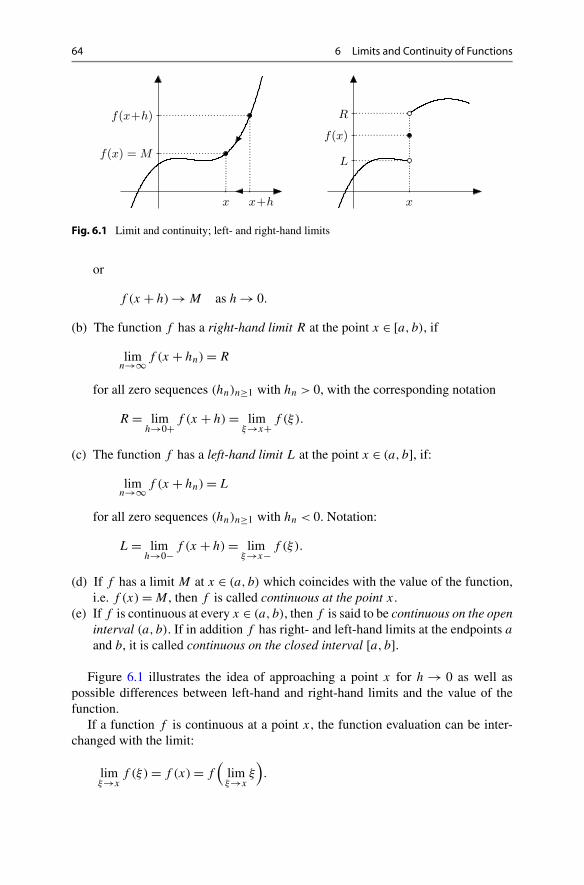
64 6 Limits and Continuity of Functions
Fig. 6.1 Limit and continuity; left- and right-hand limits
or
f (x + h) → M as h → 0.
(b) The function f has a right-hand limit R at the point x ∈ [a, b), if
limn→∞f (x + hn) = R
for all zero sequences (hn)n≥1 with hn > 0, with the corresponding notation
R = limh→0+f (x + h) = lim
ξ→x+f (ξ).
(c) The function f has a left-hand limit L at the point x ∈ (a, b], if:
limn→∞f (x + hn) = L
for all zero sequences (hn)n≥1 with hn < 0. Notation:
L = limh→0−f (x + h) = lim
ξ→x−f (ξ).
(d) If f has a limit M at x ∈ (a, b) which coincides with the value of the function,i.e. f (x) = M , then f is called continuous at the point x.
(e) If f is continuous at every x ∈ (a, b), then f is said to be continuous on the openinterval (a, b). If in addition f has right- and left-hand limits at the endpoints a
and b, it is called continuous on the closed interval [a, b].
Figure 6.1 illustrates the idea of approaching a point x for h → 0 as well aspossible differences between left-hand and right-hand limits and the value of thefunction.
If a function f is continuous at a point x, the function evaluation can be inter-changed with the limit:
limξ→x
f (ξ) = f (x) = f(
limξ→x
ξ).


66 6 Limits and Continuity of Functions
Fig. 6.3 Discontinuities:jump discontinuity andexceptional value
Fig. 6.4 No limits,oscillation withnon-vanishing amplitude
Example 6.7 The function f (x) = sin 1x
has no left- or right-hand limit at x = 0but oscillates with non-vanishing amplitude (Fig. 6.4). Indeed, one obtains differentlimits for different zero sequences. For example, for
hn = 1
nπ, kn = 1
π/2 + 2nπ, ln = 1
3π/2 + 2nπ
the respective limits are
limn→∞f (hn) = 0, lim
n→∞f (kn) = 1, limn→∞f (ln) = −1.
All other values in the interval [−1,1] can also be obtained as limits with the helpof suitable zero sequences.
Example 6.8 The function g(x) = x sin 1x
can be continuously extended by g(0) = 0at x = 0; it oscillates with vanishing amplitude (Fig. 6.5). Indeed,
∣∣g(hn) − g(0)∣∣ =
∣∣∣∣hn sin1
hn
− 0
∣∣∣∣ ≤ |hn| → 0
for all zero sequences (hn)n≥1; thus limh→0 h sin 1h
= 0.
Experiment 6.9 Open the M-files mat06_1.m and mat06_2.m and study thegraphs of the functions in Figs. 6.4 and 6.5 with the use of the zoom tool in thefigure window. How can you improve the accuracy of the visualisation in the neigh-bourhood of x = 0?
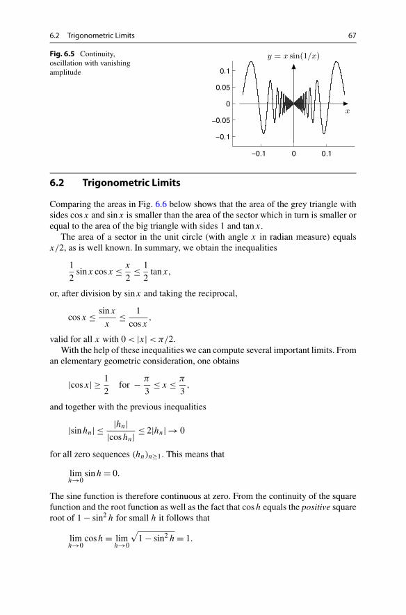
6.2 Trigonometric Limits 67
Fig. 6.5 Continuity,oscillation with vanishingamplitude
6.2 Trigonometric Limits
Comparing the areas in Fig. 6.6 below shows that the area of the grey triangle withsides cosx and sinx is smaller than the area of the sector which in turn is smaller orequal to the area of the big triangle with sides 1 and tanx.
The area of a sector in the unit circle (with angle x in radian measure) equalsx/2, as is well known. In summary, we obtain the inequalities
1
2sinx cosx ≤ x
2≤ 1
2tanx,
or, after division by sinx and taking the reciprocal,
cosx ≤ sinx
x≤ 1
cosx,
valid for all x with 0 < |x| < π/2.With the help of these inequalities we can compute several important limits. From
an elementary geometric consideration, one obtains
|cosx| ≥ 1
2for − π
3≤ x ≤ π
3,
and together with the previous inequalities
|sinhn| ≤ |hn||coshn| ≤ 2|hn| → 0
for all zero sequences (hn)n≥1. This means that
limh→0
sinh = 0.
The sine function is therefore continuous at zero. From the continuity of the squarefunction and the root function as well as the fact that cosh equals the positive squareroot of 1 − sin2 h for small h it follows that
limh→0
cosh = limh→0
√1 − sin2 h = 1.


6.3 Zeros of Continuous Functions 69
Fig. 6.7 The intermediatevalue theorem
Proof The proof is based on the successive bisection of the intervals and the com-pleteness of the set of real numbers. One starts with the interval [a, b] and setsa1 = a, b1 = b.
Step 1: Compute y1 = f(
a1+b12
).
If y1 > 0 : set a2 = a1, b2 = a1 + b1
2.
If y1 < 0 : set a2 = a1 + b1
2, b2 = b1.
If y1 = 0 : termination, ξ = a1 + b1
2is a zero.
By construction f (a2) < 0, f (b2) > 0 and the interval length is halved:
b2 − a2 = 1
2(b1 − a1).
Step 2: Compute y2 = f(
a2+b22
).
If y2 > 0 : set a3 = a2, b3 = a2 + b2
2.
If y2 < 0 : set a3 = a2 + b2
2, b3 = b2.
If y2 = 0 : termination, ξ = a2 + b2
2is a zero.
Further iterations lead to a monotonically increasing sequence,
a1 ≤ a2 ≤ a3 ≤ · · · ≤ b,
which is bounded from above. According to Proposition 5.10 the limit ξ =limn→∞ an exists.
On the other hand |an − bn| ≤ |a − b|/2n−1 → 0, therefore limn→∞ bn = ξ aswell. If ξ has not appeared after a finite number of steps as either ak or bk then forall n ∈ N:
f (an) < 0, f (bn) > 0.

70 6 Limits and Continuity of Functions
From the continuity of f it follows that
f (ξ) = limn→∞f (an) ≤ 0, f (ξ) = lim
n→∞f (bn) ≥ 0,
which implies f (ξ) = 0, as claimed. �
The proof provides at the same time a numerical method to compute zeros offunctions, the bisection method. Although it converges rather slowly, it is easilyimplementable and universally applicable—also for non-differentiable, continuousfunctions. For differentiable functions, however, considerably faster algorithms ex-ist. The order of convergence and the discussion of faster procedures will be takenup in Sect. 8.2.
Example 6.12 Calculation of√
2 as the root of f (x) = x2 − 2 = 0 in the interval[1,2] using the bisection method:
Start: f (1) = −1 < 0, f (2) = 2 > 0; a1 = 1, b1 = 2.
Step 1: f (1.5) = 0.25 > 0; a2 = 1, b2 = 1.5.
Step 2: f (1.25) = −0.4375 < 0; a3 = 1.25, b3 = 1.5.
Step 3: f (1.375) = −0.109375 < 0; a4 = 1.375, b4 = 1.5.
Step 4: f (1.4375) = 0.066406 . . . > 0; a5 = 1.375, b5 = 1.4375.
Step 5: f (1.40625) = −0.022461 . . . < 0; a6 = 1.40625, b6 = 1.4375.
etc.
After five steps the first decimal place is ascertained:
1.40625 <√
2 < 1.4375.
Experiment 6.13 Sketch the graph of the function y = x3 + 3x2 − 2 on the interval[−3,2] and try to first estimate graphically one of the roots by successive bisection.Execute the interval bisection with the help of the applet Bisection method. Assureyourself of the plausibility of the intermediate value theorem using the applet Ani-mation of the intermediate value theorem.
As an important application of the intermediate value theorem we now show thatimages of intervals under continuous functions are again intervals. For the differenttypes of intervals which appear in the following proposition we refer to Sect. 1.2;for the notion of the proper range to Sect. 2.1.
Proposition 6.14 Let I ⊂ R be an interval (open, half-open or closed, bounded orimproper) and f : I → R a continuous function with proper range J = f (I). ThenJ is also an interval.
Proof As subsets of the real line, intervals are characterised by the following prop-erty: with any two points all intermediate points are contained in it as well. Lety1, y2 ∈ J , y1 < y2, and let η be an intermediate point, i.e. y1 < η < y2. Since

6.4 Exercises 71
f : I → J is surjective there are x1, x2 ∈ I such that y1 = f (x1) and y2 = f (x2).We consider the case x1 < x2. Since f (x1) − η < 0 and f (x2) − η > 0, it followsfrom the intermediate value theorem applied on the interval [x1, x2] that there existsa point ξ ∈ (x1, x2) with f (ξ)−η = 0, thus f (ξ) = η. Hence η is attained as a valueof the function and therefore lies in J = f (I). �
Proposition 6.15 Let I = [a, b] be a closed, bounded interval and f : I → R acontinuous function. Then the proper range J = f (I) is also a closed, boundedinterval.
Proof According to Proposition 6.14 the range J is an interval. Let d be the leastupper bound (possibly d = ∞). We take a sequence of values yn ∈ J which con-verges to d . The values yn are function values of certain arguments xn ∈ I = [a, b].The sequence (xn)n≥1 is bounded and, according to Proposition 5.30, has an accu-mulation point x0, a ≤ x0 ≤ b. Thus a subsequence (xnj
)j≥1 exists which convergesto x0 (see Sect. 5.4). From the continuity of the function f it follows that
d = limj→∞ynj
= limj→∞f (xnj
) = f (x0).
This shows that the upper endpoint of the interval J is finite and is attained asfunction value. The same argument is applied to the lower boundary c; the range J
is therefore a closed, bounded interval [c, d]. �
From the proof of the proposition it is clear that d is the largest and c the smallestvalue of the function f on the interval [a, b]. We thus obtain the following importantconsequence.
Corollary 6.16 Each continuous function defined on a closed interval I = [a, b]attains its maximum and minimum there.
6.4 Exercises
1. (a) Investigate the behaviour of the functions
x + x2
|x| ,
√1 + x − 1
x,
x2 + sinx√1 − cos2 x
in a neighbourhood of x = 0 by plotting their graphs for arguments in[−2,− 1
100 ) ∪ ( 1100 ,2].
(b) Find out by inspection of the graphs whether there are left- or right-handlimits at x = 0. Which value do they have? Explain your results by rearrangingthe expressions in (a).Hint. Some guidance for part (a) can be found in the M-file mat06_ex1.m.Expand the middle term in (b) with
√1 + x + 1.

72 6 Limits and Continuity of Functions
2. Do the following functions have a limit at the given points? If so, what is itsvalue?(a) y = x3 + 5x + 10, x = 1.(b) y = x2−1
x2+x, x = 0, x = 1, x = −1.
(c) y = 1−cosx
x2 , x = 0.
Hint. Expand with (1 + cosx).(d) y = signx · sinx, x = 0.(e) y = signx · cosx, x = 0.
3. Let fn(x) = arctannx, gn(x) = (1 + x2)−n. Compute the limits
f (x) = limn→∞fn(x), g(x) = lim
n→∞gn(x)
for each x ∈ R and sketch the graphs of the thereby defined functions f and g.Are they continuous? Plot fn and gn using MATLAB and investigate the behaviourof the graphs for n → ∞.Hint. An advice can be found in the M-file mat06_ex3.m.
4. With the help of zero sequences, carry out a formal proof of the fact that the ab-solute value function and the third root function of Example 6.3 are continuous.
5. Argue with the help of the intermediate value theorem that p(x) = x3 + 5x + 10has a zero in the interval [−2,1]. Compute this zero up to four decimal placesusing the applet Bisection method.
6. Compute all zeros of the following functions in the given interval with accuracy10−3, using the applet Bisection method.
f (x) = x4 − 2, I = R.
g(x) = x − cosx, I = R.
h(x) = sin1
x, I =
[1
20,
1
10
].
7. Write a MATLAB program which locates—with the help of the bisection method—the zero of an arbitrary polynomial
p(x) = x3 + c1x2 + c2x + c3
of degree three. Your program should automatically provide starting values a, b
with p(a) < 0, p(b) > 0. (Why do such values always exist?) Test your programby choosing the coefficient vector (c1, c2, c3) randomly, for example by usingc = 1000*rand(1,3).Hint. A solution is suggested in the M-file mat06_ex7a.m. In mat06_ex7b.m you can find an alternative in which the vector functions of MATLABare exploited in a more efficient way.
7The Derivative of a Function
Starting from the problem to define the tangent to the graph of a function, we in-troduce the derivative of a function. Two points on the graph can always be joinedby a secant, which is a good model for the tangent whenever these points are closeto each other. In a limiting process, the secant (discrete model) is replaced by thetangent (continuous model). Differential calculus, which is based on this limitingprocess, has become one of the most important building blocks of mathematicalmodelling.
In this section we discuss the derivative of important elementary functions aswell as general differentiation rules. Thanks to the meticulous implementation ofthese rules, expert systems such as maple have become helpful tools in mathemat-ical analysis. Furthermore, we will discuss the interpretation of the derivative aslinear approximation and as rate of change. These interpretations form the basis ofnumerous applications in science and engineering.
The concept of the numerical derivative follows the opposite direction. The con-tinuous model is discretised and the derivative is replaced by a difference quotient.We carry out a detailed error analysis which allows us to find an optimal approxima-tion. Further, we will illustrate the relevance of symmetry in numerical procedures.
7.1 Motivation
Example 7.1 (The free fall according to Galilei1) Imagine an object which, releasedat time t = 0, falls down under the influence of gravity. We are interested in theposition s(t) of the object at time t ≥ 0 as well as in its velocity v(t); see Fig. 7.1.Due to the definition of velocity as change in travelled distance divided by changein time, the object has the average velocity
vaverage = s(t + �t) − s(t)
�t
1G. Galilei, 1564–1642.
M. Oberguggenberger, A. Ostermann, Analysis for Computer Scientists,Undergraduate Topics in Computer Science,DOI 10.1007/978-0-85729-446-3_7, © Springer-Verlag London Limited 2011
73

74 7 The Derivative of a Function
Fig. 7.1 The free fall
in the time interval [t, t +�t]. In order to obtain the instantaneous velocity v = v(t)
we take the limit �t → 0 in the above formula and arrive at
v(t) = lim�t→0
s(t + �t) − s(t)
�t.
Galilei discovered through his experiments that the travelled distance in free fallincreases quadratically with the time passed, i.e., the law
s(t) = g
2t2
with g ≈ 9.81 m/s2 holds. Thus we obtain the expression
v(t) = lim�t→0
g2 (t + �t)2 − g
2 t2
�t= g
2lim
�t→0
(2t + �t
) = gt
for the instantaneous velocity. The velocity is hence proportional to the time passed.
Example 7.2 (The tangent problem) Consider a real function f and two differ-ent points P = (x0, f (x0)) and Q = (x, f (x)) on the graph of the function. Theuniquely defined straight line through these two points is called secant of the func-tion f through P and Q; see Fig. 7.2. The slope of the secant is given by the differ-ence quotient
�y
�x= f (x) − f (x0)
x − x0.
As x tends to x0, the secant graphically turns into the tangent, provided the limitexists. Motivated by this idea we define the slope
k = limx→x0
f (x) − f (x0)
x − x0= lim
h→0
f (x0 + h) − f (x0)
h
of the function f at x0. If this limit exists, we call the straight line
y = k · (x − x0) + f (x0)
the tangent to the graph of the function at the point (x0, f (x0)).

7.2 The Derivative 75
Fig. 7.2 Slope of the secant
Experiment 7.3 Plot the function f (x) = x2 on the interval [0,2] in MATLAB. Drawthe straight lines through the points (1,1), (2, z) for various values of z. Adjust z
until you find the tangent to the graph of the function f at (1,1) and read off itsslope.
7.2 The Derivative
Motivated by the above applications we are going to define the derivative of a real-valued function.
Definition 7.4 (Derivative) Let I ⊂ R be an open interval, f : I → R a real-valuedfunction and x0 ∈ I .(a) The function f is called differentiable at x0 if the difference quotient
�y
�x= f (x) − f (x0)
x − x0
has a (finite) limit for x → x0. In this case one writes
f ′(x0) = limx→x0
f (x) − f (x0)
x − x0= lim
h→0
f (x0 + h) − f (x0)
h
and calls the limit derivative of f at the point x0.(b) The function f is called differentiable (in the interval I ) if f ′(x) exists for all
x ∈ I . In this case the function
f ′ : I → R : x �→ f ′(x)
is called the derivative of f . The process of computing f ′ from f is calleddifferentiation.
In place of f ′(x) one often writes dfdx
(x) or ddx
f (x). The following examplesshow how the derivative of a function is obtained by means of the limiting processabove.

76 7 The Derivative of a Function
Example 7.5 (The constant function f (x) = c)
f ′(x) = limh→0
f (x + h) − f (x)
h= lim
h→0
c − c
h= lim
h→0
0
h= 0.
The derivative of a constant function is zero.
Example 7.6 (The affine function g(x) = ax + b)
g′(x) = limh→0
g(x + h) − g(x)
h= lim
h→0
ax + ah + b − ax − b
h= lim
h→0a = a.
The derivative is the slope a of the straight line y = ax + b.
Example 7.7 (The derivative of the quadratic function y = x2)
y′ = limh→0
(x + h)2 − x2
h= lim
h→0
2hx + h2
h= lim
h→0(2x + h) = 2x.
Similarly, one can show for the power function (with n ∈ N):
f (x) = xn ⇒ f ′(x) = n · xn−1.
Example 7.8 (The derivative of the square root function y = √x for x > 0)
y′ = limξ→x
√ξ − √
x
ξ − x= lim
ξ→x
√ξ − √
x
(√
ξ − √x)(
√ξ + √
x)= lim
ξ→x
1√ξ + √
x= 1
2√
x.
Example 7.9 (Derivatives of the sine and cosine functions) We first recall fromProposition 6.10 that
limt→0
sin t
t= 1.
Due to
(cos t − 1)(cos t + 1) = − sin2 t
also the following holds:
cos t − 1
t= − sin t︸︷︷︸
→0
· sin t
t︸︷︷︸→1
· 1
cos t + 1︸ ︷︷ ︸→1/2
→ 0 for t → 0,
and thus
limt→0
cos t − 1
t= 0.
7.2 The Derivative 77
Due to the addition theorems (Proposition 3.3) we get with the preparations fromabove
sin′ x = limh→0
sin(x + h) − sinx
h= lim
h→0
sinx cosh + cosx sinh − sinx
h
= limh→0
sinx · cosh − 1
h+ lim
h→0cosx · sinh
h
= sinx · limh→0
cosh − 1
h︸ ︷︷ ︸=0
+ cosx · limh→0
sinh
h︸ ︷︷ ︸=1
= cosx.
This proves the formula sin′ x = cosx. Likewise it can be shown that cos′ x =− sinx.
Example 7.10 (The derivative of the exponential function with base e) Rearrangingterms in the series expansion of the exponential function (Proposition 24.12) weobtain
eh − 1
h=
∞∑k=0
hk
(k + 1)! = 1 + h
2+ h2
6+ h3
24+ · · · .
From this one infers∣∣∣∣eh − 1
h− 1
∣∣∣∣ ≤ |h|(
1
2+ |h|
6+ |h|3
24+ · · ·
)≤ |h|e|h|.
Letting h → 0 hence gives the important limit
limh→0
eh − 1
h= 1.
The existence of the limit
limh→0
ex+h − ex
h= ex · lim
h→0
eh − 1
h= ex
shows that the exponential function is differentiable and that (ex)′ = ex .
Example 7.11 (New representation of Euler’s number) By substituting y = eh − 1,h = log(y + 1) in the above limit one obtains
limy→0
y
log(y + 1)= 1
and in this way
limy→0
log(1 + αy)1/y = limy→0
log(1 + αy)
y= α lim
y→0
log(1 + αy)
αy= α.


7.3 Interpretations of the Derivative 79
Definition 7.14 If the function f ′ is again differentiable then
f ′′(x) = d2
dx2f (x) = d2f
dx2(x) = lim
h→0
f ′(x + h) − f ′(x)
h
is called the second derivative of f with respect to x. Likewise higher derivativesare defined recursively as
f ′′′(x) = (f ′′(x)
)′ ord3
dx3f (x) = d
dx
(d2
dx2f (x)
), etc.
Differentiating with maple Using maple one can differentiate expressions aswell as functions. If the expression g is of the form
g := x^2 - a*x;
then the corresponding function f is defined by
f := x -> x^2 - a*x;
The evaluation of functions generates expressions, for example f(t) produces theexpression t2 − at . Conversely, expressions can be converted to functions usingunapply
h := unapply(g,x);
The derivative of expressions can be obtained using diff, those of functions us-ing D. Examples can be found in the maple worksheet mp07_1.mws.
7.3 Interpretations of the Derivative
We introduced the derivative geometrically as the slope of the tangent, and we sawthat the tangent to a graph of a differentiable function f at the point (x0, f (x0)) isgiven by
y = f ′(x0)(x − x0) + f (x0).
Example 7.15 Let f (x) = x4 + 1 with derivative f ′(x) = 4x3.(i) The tangent to the graph of f at the point (0,1) is
y = f ′(0) · (x − 0) + f (0) = 1
and thus horizontal.
(ii) The tangent to the graph of f at the point (1,2) is
y = f ′(1)(x − 1) + 2 = 4(x − 1) + 2 = 4x − 2.
The derivative allows further interpretations.

80 7 The Derivative of a Function
Interpretation as Linear Approximation We start off by emphasising that everydifferentiable function f can be written in the form
f (x) = f (x0) + f ′(x0)(x − x0) + R(x, x0),
where the remainder R(x, x0) has the property
limx→x0
R(x, x0)
x − x0= 0.
This follows immediately from
R(x, x0) = f (x) − f (x0) − f ′(x0)(x − x0)
by dividing by x − x0, since
f (x) − f (x0)
x − x0→ f ′(x0) as x → x0.
Application 7.16 As we have just seen, a differentiable function f is characterisedby the property that
f (x) = f (x0) + f ′(x0)(x − x0) + R(x, x0),
where the remainder term R(x, x0) tends faster to zero than x − x0. Taking thelimit x → x0 in this equation shows in particular that every differentiable functionis continuous.
Application 7.17 Let g be the function given by
g(x) = k · (x − x0) + f (x0).
Its graph is the straight line with slope k passing through the point (x0, f (x0)). Since
f (x) − g(x)
x − x0= f (x) − f (x0) − k · (x − x0)
x − x0= f ′(x0) − k + R(x, x0)
x − x0︸ ︷︷ ︸→0
as x → x0, the tangent with k = f ′(x0) is the straight line which approximates thegraph best. One therefore calls
g(x) = f (x0) + f ′(x0) · (x − x0)
the linear approximation to f at x0. For x close to x0 one can consider g(x) as agood approximation to f (x). In applications the (possibly complicated) function f
is often replaced by its linear approximation g which is easier to handle.
7.3 Interpretations of the Derivative 81
Example 7.18 Let f (x) = √x = x1/2. Consequently,
f ′(x) = 1
2x− 1
2 = 1
2√
x.
We want to find the linear approximation to the function f at x0 = a. According tothe formula above the following holds:
√x ≈ g(x) = √
a + 1
2√
a(x − a)
for x close to a, or, alternatively with h = x − a,
√a + h ≈ √
a + 1
2√
ah for small h.
If we now substitute a = 1 and h = 0.1, we obtain the approximation
√1.1 ≈ 1 + 0.1
2= 1.05.
The first digits of the actual value are 1.0488 . . . .
Physical Interpretation as Rate of Change In physical applications the deriva-tive often plays the role of a rate of change. A well-known example from everydaylife is the velocity; see Sect. 7.1. Consider a particle which is moving along a straightline. Let s(t) be the position where the particle is at time t . The average velocity isgiven by the quotient
s(t) − s(t0)
t − t0(difference in displacement divided by difference in time).
In the limit t → t0 the average velocity turns into the instantaneous velocity
v(t0) = ds
dt(t0) = s(t0) = lim
t→t0
s(t) − s(t0)
t − t0.
Note that one often writes f (t) instead of f ′(t) if the time t is the argument of thefunction f . In particular, in physics this dot notation is most commonly used.
Likewise one obtains the acceleration by differentiating the velocity
a(t) = v(t) = s(t).
The notion of velocity is also used in the modelling of other processes that vary overtime, e.g., for growth or decay.

82 7 The Derivative of a Function
7.4 Differentiation Rules
In this section I ⊂ R denotes an open interval. We first note that differentiation is alinear process.
Proposition 7.19 (Linearity of the derivative) Let f,g : I → R be two functionswhich are differentiable at x ∈ I and take c ∈ R. Then the functions f + g and c · fare differentiable at x as well and
(f (x) + g(x)
)′ = f ′(x) + g′(x),(cf (x))′ = cf ′(x).
Proof The result follows from the corresponding rules for limits. The first statementis true because
f (x + h) + g(x + h) − (f (x) + g(x))
h= f (x + h) − f (x)
h︸ ︷︷ ︸→f ′(x)
+ g(x + h) − g(x)
h︸ ︷︷ ︸→g′(x)
as h → 0. The second statement follows similarly. �
Linearity together with the differentiation rule (xm)′ = mxm−1 for powers implythat every polynomial is differentiable. Let
p(x) = anxn + an−1x
n−1 + · · · + a1x + a0.
Then its derivative has the form
p′(x) = nanxn−1 + (n − 1)an−1x
n−2 + · · · + a1.
For example, (3x7 − 4x2 + 5x − 1)′ = 21x6 − 8x + 5.The following two rules allow one to determine the derivative of products and
quotients of functions from their factors.
Proposition 7.20 (Product rule) Let f,g : I → R be two functions which are dif-ferentiable at x ∈ I . Then the function f · g is differentiable at x and
(f (x) · g(x)
)′ = f ′(x) · g(x) + f (x) · g′(x).
Proof This fact follows again from the corresponding rules for limits:
f (x + h) · g(x + h) − f (x) · g(x)
h
= f (x + h) · g(x + h) − f (x) · g(x + h)
h+ f (x) · g(x + h) − f (x) · g(x)
h

7.4 Differentiation Rules 83
= f (x + h) − f (x)
h︸ ︷︷ ︸→f ′(x)
·g(x + h)︸ ︷︷ ︸→g(x)
+ f (x) · g(x + h) − g(x)
h︸ ︷︷ ︸→g′(x)
as h → 0. The required continuity of g at x is a consequence of Application 7.16. �
Proposition 7.21 (Quotient rule) Let f,g : I → R be two functions differentiable
at x ∈ I and g(x) = 0. Then the quotient fg
is differentiable at the point x and
(f (x)
g(x)
)′= f ′(x) · g(x) − f (x) · g′(x)
g(x)2.
In particular,
(1
g(x)
)′= − g′(x)
(g(x))2.
The proof is similar to the one for the product rule and can be found in [3,Chap. 3.1], for example.
Example 7.22 An application of the quotient rule to tanx = sinxcosx
shows that
tan′ x = cos2 x + sin2 x
cos2 x= 1
cos2 x= 1 + tan2 x.
Complicated functions can often be written as a composition of simpler func-tions. For example, the function
h : [2,∞) → R : x �→ h(x) = √log(x − 1)
can be interpreted as h(x) = f (g(x)) with
f : [0,∞) → R : y �→ √y,
g : [2,∞) → [0,∞) : x �→ log(x − 1).
One denotes the composition of the functions f and g by h = f ◦ g. The followingproposition shows how such compound functions can be differentiated.
Proposition 7.23 (Chain rule) The composition of two differentiable functionsg : I → B and f : B → R is also differentiable and
d
dxf
(g(x)
) = f ′(g(x)) · g′(x).
In short-hand notation the rule is
(f ◦ g)′ = (f ′ ◦ g) · g′.

84 7 The Derivative of a Function
Proof We write
1
h
(f
(g(x + h)
) − f(g(x)
)) = f (g(x + h)) − f (g(x))
g(x + h) − g(x)· g(x + h) − g(x)
h
= f (g(x) + k) − f (g(x))
k· g(x + h) − g(x)
h,
where, due to the interpretation as a linear approximation (see Sect. 7.3), the expres-sion
k = g(x + h) − g(x)
is of the form
k = g′(x)h + R(x + h,x)
and tends to zero itself as h → 0. It follows that
d
dxf
(g(x)
) = limh→0
1
h
(f
(g(x + h)
) − f(g(x)
))
= limh→0
(f (g(x) + k) − f (g(x))
k· g(x + h) − g(x)
h
)
= f ′(g(x)) · g′(x),
and hence the assertion of the proposition follows. �
The differentiation of a composite function h(x) = f (g(x)) is consequently per-formed in three steps:1. Identify the outer function f and the inner function g with h(x) = f (g(x)).2. Differentiate the outer function f at the point g(x), i.e., compute f ′(y) and then
substitute y = g(x). The result is f ′(g(x)).3. Take the inner derivative, i.e., differentiate the inner function g and multiply it
with the result of step 2. One obtains h′(x) = f ′(g(x)) · g′(x).In the case of three or more compositions, the above rules have to be applied recur-sively.
Example 7.24 (a) Let h(x) = (sinx)3. We identify the outer function f (y) = y3
and the inner function g(x) = sinx. Then
h′(x) = 3(sinx)2 · cosx.
(b) Let h(x) = e−x2. We identify f (y) = ey and g(x) = −x2. Thus
h′(x) = e−x2 · (−2x).
The last rule that we will discuss concerns the differentiation of the inverse of adifferentiable function.

7.4 Differentiation Rules 85
Fig. 7.4 Derivative of the inverse function with detailed view of the slopes
Proposition 7.25 (Inverse function rule) Let f : I → J be bijective, differentiableand f ′(y) = 0 for all y ∈ I . Then f −1 : J → I is also differentiable and
d
dxf −1(x) = 1
f ′(f −1(x)).
In short-hand notation this rule is
(f −1)′ = 1
f ′ ◦ f −1.
Proof We set y = f −1(x) and η = f −1(ξ). Due to the continuity of the inversefunction (see Proposition 24.3) we see that η → y as ξ → x. It thus follows that
d
dxf −1(x) = lim
ξ→x
f −1(ξ) − f −1(x)
ξ − x= lim
η→y
η − y
f (η) − f (y)
= limη→y
(f (η) − f (y)
η − y
)−1
= 1
f ′(y)= 1
f ′(f −1(x)),
and hence the statement of the proposition follows. �
Figure 7.4 shows the geometric background of the inverse function rule. Theslope of a straight line in x-direction is the inverse of the slope in y-direction.
If it is known beforehand that the inverse function is differentiable, then itsderivative can also be obtained in the following way. One differentiates the iden-tity
x = f(f −1(x)
)
with respect to x using the chain rule. This yields
1 = f ′(f −1(x)) · (f −1)′
(x)
and one obtains the inverse rule by division by f ′(f −1(x)).

86 7 The Derivative of a Function
Example 7.26 (Derivative of the logarithm) Since y = logx is the inverse functionto x = ey , it follows from the inverse function rule that
(logx)′ = 1
elogx= 1
x
for x > 0. Furthermore
log |x| ={
logx, x > 0,
log(−x), x < 0
and thus
(log |x|)′ =
{(logx)′ = 1
x, x > 0,
(log(−x))′ = 1(−x)
· (−1) = 1x, x < 0.
Altogether one obtains the formula
(log |x|)′ = 1
xfor x = 0.
For logarithms to the base a one has
loga x = logx
loga, thus
(loga x
)′ = 1
x loga.
Example 7.27 (Derivatives of general power functions) From xa = ea logx we inferby the chain rule that
(xa
)′ = ea logx · a
x= xa · a
x= axa−1.
Example 7.28 (Derivative of the general exponential function) For a > 0 we haveax = ex loga . An application of the chain rule shows that
(ax
)′ = (ex loga
)′ = ex loga · loga = ax loga.
Example 7.29 For x > 0 we have xx = ex logx and thus
(xx
)′ = ex logx
(logx + x
x
)= xx(logx + 1).
Example 7.30 (Derivatives of cyclometric functions) We recall the differentiationrules for the trigonometric functions on their principal branches:
(sinx)′ = cosx =√
1 − sin2 x, −π
2≤ x ≤ π
2,
(cosx)′ = − sinx = −√
1 − cos2 x, 0 ≤ x ≤ π,
(tanx)′ = 1 + tan2 x, −π
2< x <
π
2.
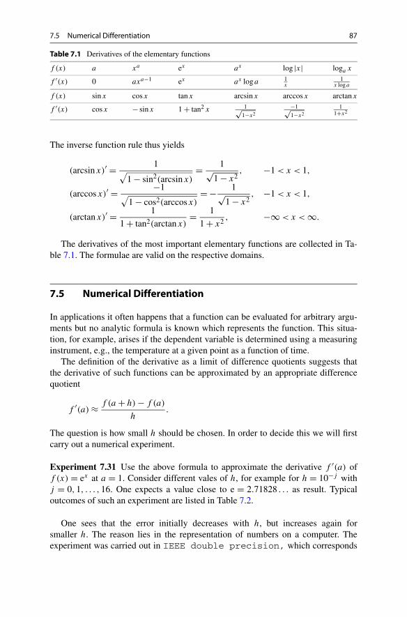
7.5 Numerical Differentiation 87
Table 7.1 Derivatives of the elementary functions
f (x) a xa ex ax log |x| loga x
f ′(x) 0 axa−1 ex ax loga 1x
1x loga
f (x) sinx cosx tanx arcsinx arccosx arctanx
f ′(x) cosx − sinx 1 + tan2 x 1√1−x2
−1√1−x2
11+x2
The inverse function rule thus yields
(arcsinx)′ = 1√1 − sin2(arcsinx)
= 1√1 − x2
, −1 < x < 1,
(arccosx)′ = −1√1 − cos2(arccosx)
= − 1√1 − x2
, −1 < x < 1,
(arctanx)′ = 1
1 + tan2(arctanx)= 1
1 + x2, −∞ < x < ∞.
The derivatives of the most important elementary functions are collected in Ta-ble 7.1. The formulae are valid on the respective domains.
7.5 Numerical Differentiation
In applications it often happens that a function can be evaluated for arbitrary argu-ments but no analytic formula is known which represents the function. This situa-tion, for example, arises if the dependent variable is determined using a measuringinstrument, e.g., the temperature at a given point as a function of time.
The definition of the derivative as a limit of difference quotients suggests thatthe derivative of such functions can be approximated by an appropriate differencequotient
f ′(a) ≈ f (a + h) − f (a)
h.
The question is how small h should be chosen. In order to decide this we will firstcarry out a numerical experiment.
Experiment 7.31 Use the above formula to approximate the derivative f ′(a) off (x) = ex at a = 1. Consider different vales of h, for example for h = 10−j withj = 0,1, . . . ,16. One expects a value close to e = 2.71828 . . . as result. Typicaloutcomes of such an experiment are listed in Table 7.2.
One sees that the error initially decreases with h, but increases again forsmaller h. The reason lies in the representation of numbers on a computer. Theexperiment was carried out in IEEE double precision, which corresponds

88 7 The Derivative of a Function
Table 7.2 Numerical differentiation of the exponential function at a = 1 using a one-sided differ-ence quotient. The numerical results and errors are given as functions of h
h value error
1.000E-000 4.67077427047160 1.95249244201256E-000
1.000E-001 2.85884195487388 1.40560126414838E-001
1.000E-002 2.73191865578714 1.36368273280976E-002
1.000E-003 2.71964142253338 1.35959407433051E-003
1.000E-004 2.71841774708220 1.35918623152431E-004
1.000E-005 2.71829541994577 1.35914867218645E-005
1.000E-006 2.71828318752147 1.35906242526573E-006
1.000E-007 2.71828196740610 1.38947053418548E-007
1.000E-008 2.71828183998415 1.15251088672608E-008
1.000E-009 2.71828219937549 3.70916445113778E-007
1.000E-010 2.71828349976758 1.67130853068187E-006
1.000E-011 2.71829650802524 1.46795661959409E-005
1.000E-012 2.71866817252997 3.86344070924416E-004
1.000E-013 2.71755491373926 -7.26914719783700E-004
1.000E-014 2.73058485544819 1.23030269891471E-002
1.000E-015 3.16240089670572 4.44119068246674E-001
1.000E-016 1.44632569809566 -1.27195613036338E-000
to a relative machine accuracy of eps ≈ 10−16. The experiment shows that the bestresult is obtained for
h ≈ √eps≈ 10−8.
This behaviour can be explained by using a Taylor expansion. In Chap. 12 we willderive the formula
f (a + h) = f (a) + hf ′(a) + h2
2f ′′(ξ),
where ξ denotes an appropriate point between a and a+h. (The value of ξ is usuallynot known.) Thus, after rearranging, we get
f ′(a) = f (a + h) − f (a)
h− h
2f ′′(ξ).
The discretisation error, i.e., the error which arises from replacing the derivative bythe difference quotient, is proportional to h and decreases linearly with h. This be-haviour can also be seen in the numerical experiment for h between 10−2 and 10−8.

7.5 Numerical Differentiation 89
Fig. 7.5 Approximation ofthe tangent by a symmetricsecant
For very small h, rounding errors additionally come into play. As we have seenin Sect. 1.4 the calculation of f (a) on a computer yields
rd(f (a)
) = f (a) · (1 + ε) = f (a) + εf (a)
with |ε| ≤ eps. The rounding error turns out to be proportional to eps/h andincreases dramatically for small h. This behaviour can be seen in the numericalexperiment for h between 10−8 and 10−16.
The result of the numerical derivative using the one-sided difference quotient
f ′(a) ≈ f (a + h) − f (a)
h
is then most precise if the discretisation and rounding errors have approximately thesame magnitude, so if
h ≈ eps
hor h ≈ √
eps≈ 10−8.
In order to calculate the derivative of f ′(a) one can also use a secant placedsymmetrically around (a, f (a)), i.e.,
f ′(a) = limh→0
f (a + h) − f (a − h)
2h.
This suggests the symmetric formula (see Fig. 7.5)
f ′(a) ≈ f (a + h) − f (a − h)
2h.
This approximation is called symmetric difference quotient.To analyse the accuracy of the approximation, we need the Taylor series from
Chap. 12:
f (a + h) = f (a) + hf ′(a) + h2
2f ′′(a) + h3
6f ′′′(a) + · · · .
If one replaces h by −h in this formula
f (a − h) = f (a) − hf ′(a) + h2
2f ′′(a) − h3
6f ′′′(a) + · · ·

90 7 The Derivative of a Function
Table 7.3 Numerical differentiation of the exponential function at a = 1 using a symmetric dif-ference quotient. The numerical results and errors are given as functions of h
h value error
1.000E-000 3.19452804946533 4.76246221006280E-001
1.000E-001 2.72281456394742 4.53273548837307E-003
1.000E-002 2.71832713338270 4.53049236583958E-005
1.000E-003 2.71828228150582 4.53046770765297E-007
1.000E-004 2.71828183298958 4.53053283777649E-009
1.000E-005 2.71828182851255 5.35020916458961E-011
1.000E-006 2.71828182834134 -1.17704512803130E-010
1.000E-007 2.71828182903696 5.77919490041268E-010
1.000E-008 2.71828181795317 -1.05058792776447E-008
1.000E-009 2.71828182478364 -3.67540575751946E-009
1.000E-010 2.71828199164235 1.63183308643511E-007
1.000E-011 2.71829103280427 9.20434522511116E-006
1.000E-012 2.71839560410381 1.13775644761560E-004
and takes the difference, one obtains
f (a + h) − f (a − h) = 2hf ′(a) + 2h3
6f ′′′(a) + · · ·
and furthermore
f ′(a) = f (a + h) − f (a − h)
2h− h2
6f ′′′(a) + · · · .
In this case the discretisation error is hence proportional to h2, while the roundingerror is still proportional to eps/h.
The symmetric procedure thus delivers the best results for
h2 ≈ eps
hor h ≈ 3
√eps,
respectively. We repeat Experiment 7.31 with f (x) = ex, a = 1 and h = 10−j forj = 0, . . . ,12. The results are listed in Table 7.3.
As expected one obtains the best result for h ≈ 10−5. The obtained approxima-tion is more precise than that of Table 7.2. Since symmetric procedures generallygive better results, symmetry is an important concept in numerical mathematics.
Numerical Differentiation of Noisy Functions In practice, it often occurs that afunction which has to be differentiated consists of discrete data that are addition-ally perturbed by noise. The noise represents small measuring errors and behavesstatistically like random numbers.

7.5 Numerical Differentiation 91
Fig. 7.6 The left picture shows random noise which masks the data. The noise is modelled by 801normally distributed random numbers. The frequencies of the chosen random numbers can be seenin the histogram in the right picture. For comparison, the (scaled) density of the correspondingnormal distribution is given there as well
Example 7.32 Digitising a line of a picture by J + 1 pixels produces a function
f : {0,1, . . . , J } → R : j �→ f (j) = fj = brightness of thej th pixel.
In order to find an edge in the picture, where the brightness locally changes veryrapidly, this function has to be differentiated.
We consider a concrete example. Suppose that the picture information consistsof the function
g : [a, b] → R : x �→ g(x) = −2x3 + 4x
with a = −2 and b = 2. Let �x be the distance between two pixels and
J = b − a
�x
denote the total number of pixels minus 1. We choose �x = 1/200 and thus obtainJ = 800. The actual brightness of the j th pixel would then be
gj = g(a + j�x), 0 ≤ j ≤ J.
However, due to measuring errors the measuring instrument supplies
fj = gj + εj ,
where εj are random numbers. We choose normally distributed random numberswith expected value 0 and variance 2.5 · 10−5 for εj ; see Fig. 7.6. For an exactdefinition of the notions of expected value and variance we refer to the literature,for instance [17].
These random numbers can be generated in MATLAB using the command
randn(1,801)*sqrt(2.5e-5).
Differentiating f using the previous rules generates
f ′j ≈ fj − fj−1
�x= gj − gj−1
�x+ εj − εj−1
�x
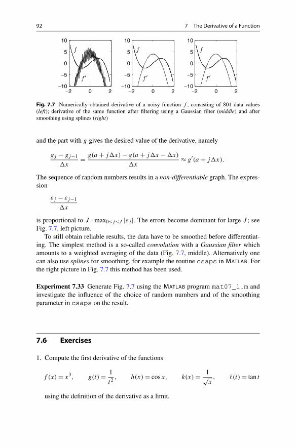
92 7 The Derivative of a Function
Fig. 7.7 Numerically obtained derivative of a noisy function f , consisting of 801 data values(left); derivative of the same function after filtering using a Gaussian filter (middle) and aftersmoothing using splines (right)
and the part with g gives the desired value of the derivative, namely
gj − gj−1
�x= g(a + j�x) − g(a + j�x − �x)
�x≈ g′(a + j�x).
The sequence of random numbers results in a non-differentiable graph. The expres-sion
εj − εj−1
�x
is proportional to J · max0≤j≤J |εj |. The errors become dominant for large J ; seeFig. 7.7, left picture.
To still obtain reliable results, the data have to be smoothed before differentiat-ing. The simplest method is a so-called convolution with a Gaussian filter whichamounts to a weighted averaging of the data (Fig. 7.7, middle). Alternatively onecan also use splines for smoothing, for example the routine csaps in MATLAB. Forthe right picture in Fig. 7.7 this method has been used.
Experiment 7.33 Generate Fig. 7.7 using the MATLAB program mat07_1.m andinvestigate the influence of the choice of random numbers and of the smoothingparameter in csaps on the result.
7.6 Exercises
1. Compute the first derivative of the functions
f (x) = x3, g(t) = 1
t2, h(x) = cosx, k(x) = 1√
x, �(t) = tan t
using the definition of the derivative as a limit.
7.6 Exercises 93
2. Compute the first derivative of the functions
a(x) = x2 − 1
x2 + 2x + 1, b(t) = t2ecos(t2+1),
c(x) = x2 sinx, d(s) = log(s +
√1 + s2
).
Check your results with maple.3. Compute an approximation of
√34 by replacing the function f (x) = √
x atx = 36 by its linear approximation. How accurate is your result?
4. Show that the functions f (x) = arctanx and g(x) = arctan 1+x1−x
differ in the in-terval (−∞,1) by a constant. Compute this constant. Answer the same questionfor the interval (1,∞).
5. Sand runs from a conveyor belt onto a heap with a velocity of 2 m3/min. Thesand forms a cone-shaped pile whose height equals 4
3 of the radius. With whichvelocity does the radius grow if the sand cone has a diameter of 6 m?Hint. Determine the volume V as a function of the radius r , consider V and r asfunctions of time t and differentiate the equation with respect to t . Compute r .
6. Use the Taylor series
y(x + h) = y(x) + hy′(x) + h2
2y′′(x) + h3
6y′′′(x) + h4
24y(4)(x) + · · ·
to derive the formula
y′′(x) = y(x + h) − 2y(x) + y(x − h)
h2− h2
12y(4)(x) + · · ·
and read off from this expression a numerical method for calculating the secondderivative. The discretisation error is proportional to h2, the rounding error isproportional to eps/h2. By equating the discretisation and the rounding errordeduce the optimal step size h. Check your considerations by performing a nu-merical experiment in MATLAB, computing the second derivative of y(x) = e2x
at the point x = 1.7. Write a MATLAB program which numerically differentiates a given function on a
given interval and plots the function and its first derivative. Test your program onthe functions
f (x) = cosx, 0 ≤ x ≤ 6π,
and
g(x) = e− cos(3x), 0 ≤ x ≤ 2.

8Applications of the Derivative
This chapter is devoted to some applications of the derivative which form part of thebasic skills in modelling. We start with a discussion of features of graphs. More pre-cisely, we use the derivative to describe geometric properties like maxima, minimaand monotonicity. Even though plotting functions with MATLAB or maple is simple,understanding the connection with the derivative is important, for example, when afunction with given properties is to be chosen from a particular class of functions.
In the following section we discuss Newton’s method and the concept of orderof convergence. Newton’s method is one of the most important tools for computingzeros of functions. It is nearly universally in use.
The final section of this chapter is devoted to an elementary method from dataanalysis. We show how to compute a regression line through the origin. There aremany areas of application that involve linear regression. This topic will be developedin more detail in Chap. 18.
8.1 Curve Sketching
In the following we investigate some geometric properties of graphs of functionsusing the derivative: maxima and minima, intervals of monotonicity, and convexity.We further discuss the mean value theorem which is an important technical tool forproofs.
Definition 8.1 A function f : [a, b] → R has(a) a global maximum at x0 ∈ [a, b] if
f (x) ≤ f (x0) for all x ∈ [a, b]
(b) a local maximum at x0 ∈ [a, b], if there exists a neighbourhood Uε(x0) so that
f (x) ≤ f (x0) for all x ∈ Uε(x0) ∩ [a, b].M. Oberguggenberger, A. Ostermann, Analysis for Computer Scientists,Undergraduate Topics in Computer Science,DOI 10.1007/978-0-85729-446-3_8, © Springer-Verlag London Limited 2011
95
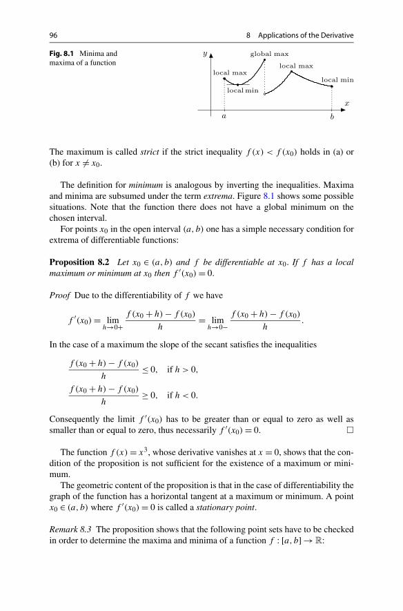
96 8 Applications of the Derivative
Fig. 8.1 Minima andmaxima of a function
The maximum is called strict if the strict inequality f (x) < f (x0) holds in (a) or(b) for x �= x0.
The definition for minimum is analogous by inverting the inequalities. Maximaand minima are subsumed under the term extrema. Figure 8.1 shows some possiblesituations. Note that the function there does not have a global minimum on thechosen interval.
For points x0 in the open interval (a, b) one has a simple necessary condition forextrema of differentiable functions:
Proposition 8.2 Let x0 ∈ (a, b) and f be differentiable at x0. If f has a localmaximum or minimum at x0 then f ′(x0) = 0.
Proof Due to the differentiability of f we have
f ′(x0) = limh→0+
f (x0 + h) − f (x0)
h= lim
h→0−f (x0 + h) − f (x0)
h.
In the case of a maximum the slope of the secant satisfies the inequalities
f (x0 + h) − f (x0)
h≤ 0, if h > 0,
f (x0 + h) − f (x0)
h≥ 0, if h < 0.
Consequently the limit f ′(x0) has to be greater than or equal to zero as well assmaller than or equal to zero, thus necessarily f ′(x0) = 0. �
The function f (x) = x3, whose derivative vanishes at x = 0, shows that the con-dition of the proposition is not sufficient for the existence of a maximum or mini-mum.
The geometric content of the proposition is that in the case of differentiability thegraph of the function has a horizontal tangent at a maximum or minimum. A pointx0 ∈ (a, b) where f ′(x0) = 0 is called a stationary point.
Remark 8.3 The proposition shows that the following point sets have to be checkedin order to determine the maxima and minima of a function f : [a, b] → R:
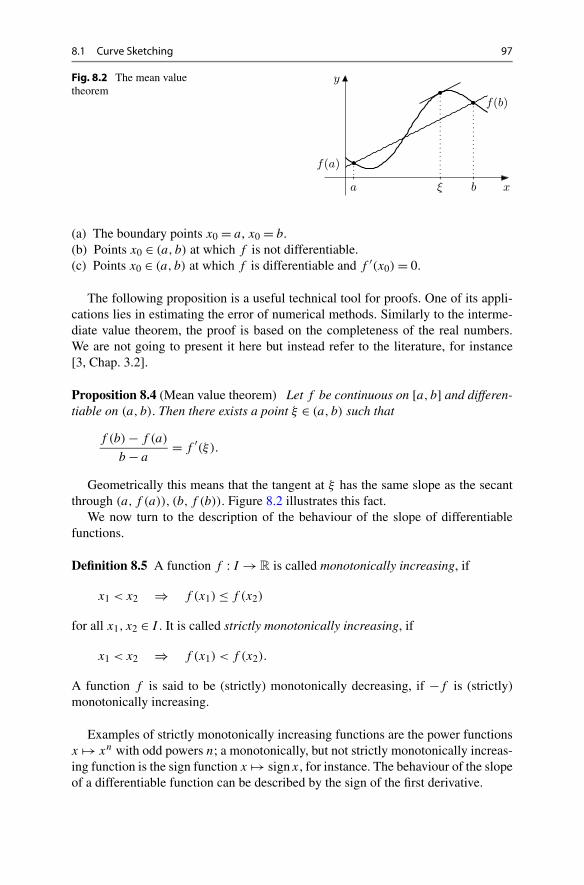
8.1 Curve Sketching 97
Fig. 8.2 The mean valuetheorem
(a) The boundary points x0 = a, x0 = b.(b) Points x0 ∈ (a, b) at which f is not differentiable.(c) Points x0 ∈ (a, b) at which f is differentiable and f ′(x0) = 0.
The following proposition is a useful technical tool for proofs. One of its appli-cations lies in estimating the error of numerical methods. Similarly to the interme-diate value theorem, the proof is based on the completeness of the real numbers.We are not going to present it here but instead refer to the literature, for instance[3, Chap. 3.2].
Proposition 8.4 (Mean value theorem) Let f be continuous on [a, b] and differen-tiable on (a, b). Then there exists a point ξ ∈ (a, b) such that
f (b) − f (a)
b − a= f ′(ξ).
Geometrically this means that the tangent at ξ has the same slope as the secantthrough (a, f (a)), (b, f (b)). Figure 8.2 illustrates this fact.
We now turn to the description of the behaviour of the slope of differentiablefunctions.
Definition 8.5 A function f : I → R is called monotonically increasing, if
x1 < x2 ⇒ f (x1) ≤ f (x2)
for all x1, x2 ∈ I . It is called strictly monotonically increasing, if
x1 < x2 ⇒ f (x1) < f (x2).
A function f is said to be (strictly) monotonically decreasing, if −f is (strictly)monotonically increasing.
Examples of strictly monotonically increasing functions are the power functionsx → xn with odd powers n; a monotonically, but not strictly monotonically increas-ing function is the sign function x → signx, for instance. The behaviour of the slopeof a differentiable function can be described by the sign of the first derivative.
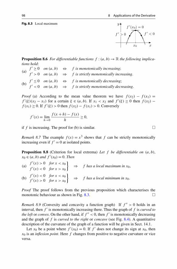
98 8 Applications of the Derivative
Fig. 8.3 Local maximum
Proposition 8.6 For differentiable functions f : (a, b) → R the following implica-tions hold:
(a)f ′ ≥ 0 on (a, b) ⇔ f is monotonically increasing;f ′ > 0 on (a, b) ⇒ f is strictly monotonically increasing.
(b)f ′ ≤ 0 on (a, b) ⇔ f is monotonically decreasing;f ′ < 0 on (a, b) ⇒ f is strictly monotonically decreasing.
Proof (a) According to the mean value theorem we have f (x2) − f (x1) =f ′(ξ)(x2 − x1) for a certain ξ ∈ (a, b). If x1 < x2 and f ′(ξ) ≥ 0 then f (x2) −f (x1) ≥ 0. If f ′(ξ) > 0 then f (x2) − f (x1) > 0. Conversely
f ′(x) = limh→0
f (x + h) − f (x)
h≥ 0,
if f is increasing. The proof for (b) is similar. �
Remark 8.7 The example f (x) = x3 shows that f can be strictly monotonicallyincreasing even if f ′ = 0 at isolated points.
Proposition 8.8 (Criterion for local extrema) Let f be differentiable on (a, b),x0 ∈ (a, b) and f ′(x0) = 0. Then
(a)f ′(x) > 0 for x < x0
f ′(x) < 0 for x > x0
}⇒ f has a local maximum in x0,
(b)f ′(x) < 0 for x < x0f ′(x) > 0 for x > x0
}⇒ f has a local minimum in x0.
Proof The proof follows from the previous proposition which characterises themonotonic behaviour as shown in Fig. 8.3. �
Remark 8.9 (Convexity and concavity a function graph) If f ′′ > 0 holds in aninterval, then f ′ is monotonically increasing there. Thus the graph of f is curved tothe left or convex. On the other hand, if f ′′ < 0, then f ′ is monotonically decreasingand the graph of f is curved to the right or concave (see Fig. 8.4). A quantitativedescription of the curvature of the graph of a function will be given in Sect. 14.1.
Let x0 be a point where f ′(x0) = 0. If f ′ does not change its sign at x0, thenx0 is an inflexion point. Here f changes from positive to negative curvature or viceversa.

8.1 Curve Sketching 99
Fig. 8.4Convexity/concavity andsecond derivative
Proposition 8.10 (Second derivative criterion for local extrema) Let f be twicecontinuously differentiable on (a, b), x0 ∈ (a, b) and f ′(x0) = 0.(a) If f ′′(x0) > 0 then f has a local minimum at x0.(b) If f ′′(x0) < 0 then f has a local maximum at x0.
Proof (a) Since f ′′ is continuous, f ′′(x) > 0 for all x in a neighbourhood of x0. Ac-cording to Proposition 8.6, f ′ is strictly monotonically increasing in this neighbour-hood. Because of f ′(x0) = 0 this means that f ′(x0) < 0 for x < x0 and f ′(x) > 0for x > x0; according to the criterion for local extrema, x0 is a minimum. The as-sertion (b) can be shown similarly. �
Remark 8.11 If f ′′(x0) = 0 there can either be an inflexion point or a minimumor maximum. The functions f (x) = xn, n = 2,3,4, . . . supply a typical example.In fact, they have for n even a global minimum at x = 0, and an inflexion pointfor n odd. More general functions can easily be assessed using a Taylor expansion.An extreme value criterion based on this expansion will be discussed in Applica-tion 12.14.
One of the applications of the previous propositions is curve sketching, which isthe detailed investigation of the properties of the graph of a function using differ-ential calculus. Even though graphs can easily be plotted in MATLAB or maple it isstill often necessary to check the graphical output at certain points using analyticmethods.
Experiment 8.12 Plot the function
y = x(signx − 1)(x + 1)3 + (sign(x − 1) + 1
)((x − 2)4 − 1/2
)
on the interval −2 ≤ x ≤ 3 and try to read off the local and global extrema, theinflexion points and the monotonic behaviour. Check your observations using thecriteria discussed above.
A further application of the previous propositions consists in finding extrema,i.e., solving one-dimensional optimisation problems. We illustrate this topic using astandard example.

100 8 Applications of the Derivative
Example 8.13 Which rectangle with a given perimeter has the largest area? To an-swer this question we denote the lengths of the sides of the rectangle by x and y.Then the perimeter and the area are given by
U = 2x + 2y, F = xy.
Since U is fixed, we obtain y = U/2 − x, and from that
F = x(U/2 − x),
where x can vary in the domain 0 ≤ x ≤ U/2. We want to find the maximum ofthe function F on the interval [0,U/2]. Since F is differentiable, we only have toinvestigate the boundary points and the stationary points. At the boundary pointsx = 0 and x = U/2 we have F(0) = 0 and F(U/2) = 0. The stationary points areobtained by setting the derivative to zero:
F ′(x) = U/2 − 2x = 0,
which brings us to x = U/4 with the function value F(U/4) = U2/16.As a result we find that the maximum area is obtained at x = U/4, thus in the
case of a square.
Experiment 8.14 On the website of maths online go to Applications of differentialcalculus in the gallery area and open the applet How to find a function’s extremum. Itis about maximising the area of a triangle which is inscribed in a rectangle. Study thetranslation of the geometric problem to a problem of differential calculus and curvesketching. Study the connection between geometry and analysis in an analogousway for Example 8.13 above.
8.2 Newton’s Method
With the help of differential calculus efficient numerical methods for computingzeros of differentiable functions can be constructed. One of the basic procedures isNewton’s method,1 which will be discussed in this section for the case of real-valuedfunctions f : D ⊂ R → R.
First we recall the bisection method discussed in Sect. 6.3. Consider a continuous,real-valued function f on an interval [a, b] with
f (a) < 0, f (b) > 0 or f (a) > 0, f (b) < 0.
1I. Newton, 1642–1727.

8.2 Newton’s Method 101
With the help of continued bisection of the interval, one obtains a zero ξ of f satis-fying
a = a1 ≤ a2 ≤ a3 ≤ · · · ≤ ξ ≤ · · · ≤ b3 ≤ b2 ≤ b1 = b,
where
|bn+1 − an+1| = 1
2|bn − an| = 1
4|bn−1 − an−1| = · · · = 1
2n|b1 − a1|.
If one stops after n iterations and chooses an or bn as approximation for ξ , then onegets a guaranteed error bound
|error| ≤ ϕ(n) = |bn − an|.
Note that we have
ϕ(n + 1) = 1
2ϕ(n).
The error thus decays with each iteration by (at least) a constant factor 12 and one
calls the method linearly convergent. More generally, an iteration scheme is calledconvergent of order α if there exist error bounds (ϕ(n))n≥1 and a constant C > 0such that
limn→∞
ϕ(n + 1)
(ϕ(n))α= C.
For sufficiently large n, one thus has approximately
ϕ(n + 1) ≈ C(ϕ(n)
)α.
Linear convergence (α = 1) therefore implies
ϕ(n + 1) ≈ Cϕ(n) ≈ C2ϕ(n − 1) ≈ · · · ≈ Cnϕ(1).
Plotting the logarithm of ϕ(n) against n (semi-logarithmic representation, as shownfor example in Fig. 8.6) results in a straight line:
logϕ(n + 1) ≈ n logC + logϕ(1).
If C < 1, then the error bound ϕ(n+1) tends to 0 and the number of correct decimalplaces increases with each iteration by a constant. Quadratic convergence wouldmean that the number of correct decimal places approximately doubles with eachiteration.

102 8 Applications of the Derivative
Fig. 8.5 Two steps ofNewton’s method
Derivation of Newton’s Method The aim of the construction is to obtain a pro-cedure that provides quadratic convergence (α = 2), at least if one starts sufficientlyclose to a simple zero ξ of a differentiable function. The geometric idea behindNewton’s method is simple: Once an approximation xn is chosen, one calculatesxn+1 as the intersection of the tangent to the graph of f through (xn, f (xn)) withthe x-axis; see Fig. 8.5. The equation of the tangent is given by
y = f (xn) + f ′(xn)(x − xn).
The point of intersection xn+1 with the x-axis is obtained from
0 = f (xn) + f ′(xn)(xn+1 − xn),
thus
xn+1 = xn − f (xn)
f ′(xn), n ≥ 1.
Obviously it has to be assumed that f ′(xn) �= 0. This condition is fulfilled, if f ′ iscontinuous and xn is sufficiently close to the zero ξ .
Proposition 8.15 (Convergence of Newton’s method) Let f be a real-valued func-tion, twice differentiable with a continuous second derivative. Further, let f (ξ) = 0and f ′(ξ) �= 0. Then there exists a neighbourhood Uε(ξ) such that Newton’s methodconverges quadratically to ξ for every starting value x1 ∈ Uε(ξ).
Proof Since f ′(ξ) �= 0 and f ′ is continuous, there exist a neighbourhood Uδ(ξ)
and a bound m > 0 so that |f ′(x)| ≥ m for all x ∈ Uδ(ξ). Applying the mean valuetheorem twice gives
|xn+1 − ξ | =∣∣∣∣xn − ξ − f (xn) − f (ξ)
f ′(xn)
∣∣∣∣

8.2 Newton’s Method 103
≤ |xn − ξ |∣∣∣∣1 − f ′(η)
f ′(xn)
∣∣∣∣ = |xn − ξ | |f′(xn) − f ′(η)|
|f ′(xn)|
≤ |xn − ξ |2 |f ′′(ζ )||f ′(xn)|
with η between xn and ξ and ζ between xn and η. Let M denote the maximum of|f ′′| on Uδ(ξ). Under the assumption that all iterates xn lie in the neighbourhoodUδ(ξ), we obtain the quadratic error bound
ϕ(n + 1) = |xn+1 − ξ | ≤ |xn − ξ |2 M
m= (
ϕ(n))2 M
m
for the error ϕ(n) = |xn − ξ |. Thus, the assertion of the proposition holds with theneighbourhood Uδ(ξ). Otherwise we have to decrease the neighbourhood by choos-ing an ε < δ which satisfies the inequality ε M
m≤ 1. Then
|xn − ξ | ≤ ε ⇒ |xn+1 − ξ | ≤ ε2 M
m≤ ε.
This means that if an approximate value xn lies in Uε(ξ) then so does the subsequentvalue xn+1. Since Uε(ξ) ⊂ Uδ(ξ), the quadratic error estimate from above is stillvalid. Thus the assertion of the proposition is valid with the smaller neighbourhoodUε(ξ). �
Example 8.16 In computing the root ξ = 3√
2 of x3 − 2 = 0, we compare the bisec-tion method with starting interval [−2,2] and Newton’s method with starting valuex1 = 2. The interval boundaries [an, bn] and the iterates xn are listed in Tables 8.1and 8.2, respectively. Newton’s method gives the value
3√
2 = 1.25992104989487
correct to 14 decimal places after only six iterations.
The error curves for the bisection method and Newton’s method can be seen inFig. 8.6. A semi-logarithmic representation (MATLAB command semilogy) is usedthere.
Remark 8.17 The convergence behaviour of Newton’s method depends on the con-ditions of Proposition 8.15. If the starting value x1 is too far away from the zero ξ ,then the method might diverge, oscillate or converge to a different zero. If f ′(ξ) = 0,which means the zero ξ has multiplicity > 1, then the order of convergence may bereduced.
Experiment 8.18 Open the applet Newton’s method and test—using the sinefunction—how the choice of the starting value influences the result (in the applet theright interval boundary is the initial value). Experiment with the intervals [−2, x0]

104 8 Applications of the Derivative
Table 8.1 Bisection method for calculating the third root of 2
n an bn error
1 -2.00000000000000 2.00000000000000 4.00000000000000
2 0.00000000000000 2.00000000000000 2.00000000000000
3 1.00000000000000 2.00000000000000 1.00000000000000
4 1.00000000000000 1.50000000000000 0.50000000000000
5 1.25000000000000 1.50000000000000 0.25000000000000
6 1.25000000000000 1.37500000000000 0.12500000000000
7 1.25000000000000 1.31250000000000 0.06250000000000
8 1.25000000000000 1.28125000000000 0.03125000000000
9 1.25000000000000 1.26562500000000 0.01562500000000
10 1.25781250000000 1.26562500000000 0.00781250000000
11 1.25781250000000 1.26171875000000 0.00390625000000
12 1.25976562500000 1.26171875000000 0.00195312500000
13 1.25976562500000 1.26074218750000 0.00097656250000
14 1.25976562500000 1.26025390625000 0.00048828125000
15 1.25976562500000 1.26000976562500 0.00024414062500
16 1.25988769531250 1.26000976562500 0.00012207031250
17 1.25988769531250 1.25994873046875 0.00006103515625
18 1.25991821289063 1.25994873046875 0.00003051757813
Table 8.2 Newton’s methodfor calculating the third rootof 2
n xn error
1 2.00000000000000 0.74007895010513
2 1.50000000000000 0.24007895010513
3 1.29629629629630 0.03637524640142
4 1.26093222474175 0.00101117484688
5 1.25992186056593 0.00000081067105
6 1.25992104989539 0.00000000000052
7 1.25992104989487 0.00000000000000
for x0 = 1,1.1,1.2,1.3,1.5,1.57,1.5707,1.57079 and interpret your observations.Also carry out the calculations with the same starting values with the help of theM-file mat08_2.m.
Experiment 8.19 With the help of the applet Newton’s method, study how the orderof convergence drops for multiple zeros. For this purpose, use the two polynomialfunctions given in the applet.
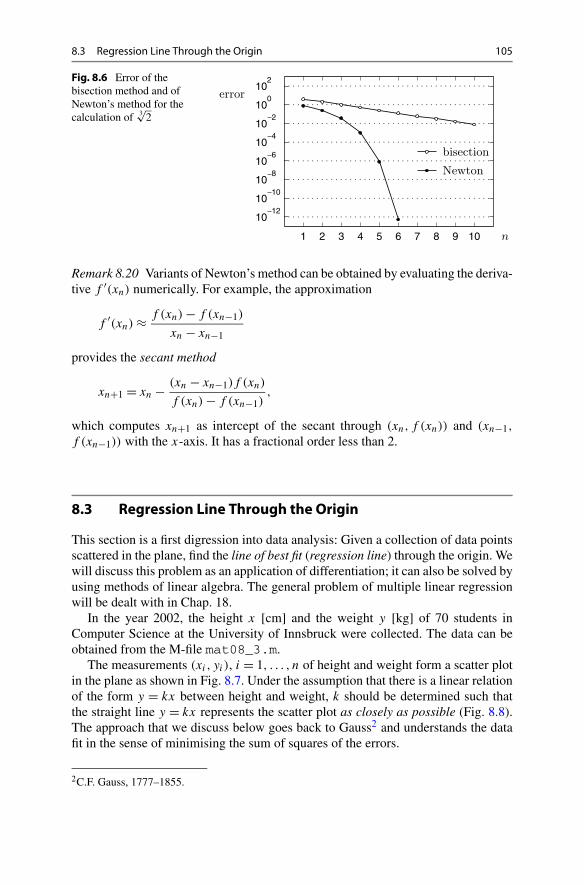
8.3 Regression Line Through the Origin 105
Fig. 8.6 Error of thebisection method and ofNewton’s method for thecalculation of 3
√2
Remark 8.20 Variants of Newton’s method can be obtained by evaluating the deriva-tive f ′(xn) numerically. For example, the approximation
f ′(xn) ≈ f (xn) − f (xn−1)
xn − xn−1
provides the secant method
xn+1 = xn − (xn − xn−1)f (xn)
f (xn) − f (xn−1),
which computes xn+1 as intercept of the secant through (xn, f (xn)) and (xn−1,
f (xn−1)) with the x-axis. It has a fractional order less than 2.
8.3 Regression Line Through the Origin
This section is a first digression into data analysis: Given a collection of data pointsscattered in the plane, find the line of best fit (regression line) through the origin. Wewill discuss this problem as an application of differentiation; it can also be solved byusing methods of linear algebra. The general problem of multiple linear regressionwill be dealt with in Chap. 18.
In the year 2002, the height x [cm] and the weight y [kg] of 70 students inComputer Science at the University of Innsbruck were collected. The data can beobtained from the M-file mat08_3.m.
The measurements (xi, yi), i = 1, . . . , n of height and weight form a scatter plotin the plane as shown in Fig. 8.7. Under the assumption that there is a linear relationof the form y = kx between height and weight, k should be determined such thatthe straight line y = kx represents the scatter plot as closely as possible (Fig. 8.8).The approach that we discuss below goes back to Gauss2 and understands the datafit in the sense of minimising the sum of squares of the errors.
2C.F. Gauss, 1777–1855.


8.3 Regression Line Through the Origin 107
By setting F ′(k) = 0 we obtain the formula
F ′(k) = −2n∑
i=1
xiyi + 2k
n∑i=1
x2i = 0.
Since evidently F ′′ > 0, its solution
k =∑
xiyi∑x2i
is the global minimum and gives the slope of the line of best fit.
Example 8.22 To illustrate the regression line through the origin we use the Austrianconsumer price index 2000–2006 (data taken from [24]):
year 2000 2001 2002 2003 2004 2005 2006index 100.0 102.7 104.5 105.9 108.1 110.6 112.2
For the calculation it is useful to introduce new variables x and y, where x = 0corresponds to the year 2000 and y = 0 to the index 100. This means that x =(year − 2000) and y = (index − 100); y describes the relative price increase (inpercent) with respect to the year 2000. The re-scaled data are
xi 0 1 2 3 4 5 6yi 0.0 2.7 4.5 5.9 8.1 10.6 12.2
We are looking for the line of best fit to these data through the origin. For thispurpose we have to minimise
F(k) = (2.7 − k · 1)2 + (4.5 − k · 2)2 + (5.9 − k · 3)2 + (8.1 − k · 4)2
+ (10.6 − k · 5)2 + (12.2 − k · 6)2,
which results in
k = 1 · 2.7 + 2 · 4.5 + 3 · 5.9 + 4 · 8.1 + 5 · 10.6 + 6 · 12.2
1 · 1 + 2 · 2 + 3 · 3 + 4 · 4 + 5 · 5 + 6 · 6= 188.0
91= 2.0659.
The line of best fit is thus
y = 2.0659x
or transformed back
index = 100 + (year − 2000) · 2.0659.
The result is shown in Fig. 8.9, in a year/index-scale as well as in the transformedvariables. For the year 2007, extrapolation along the regression line would forecast
index(2007) = 100 + 7 · 2.0659 = 114.5
(the actual consumer price index in 2007 had the value 114.6).

108 8 Applications of the Derivative
Fig. 8.9 Consumer priceindex and regression line
8.4 Exercises
1. (a) On the website of maths online go to Differentiation 1 in the gallery areaand solve the Derivative puzzles 2 and 3.(b) On the website of maths online go to Differentiation 2 in the Interactivetests area and answer the questions posed in Functions with absolute value—differentiable or not? Plot the graphs of the functions to be investigated (usingcurve sketching or MATLAB).
2. Find all maxima and minima of the functions
f (x) = x
x2 + 1and g(x) = x2e−x2
.
3. Find the maxima of the functions
y = 1
xe−(logx)2/2, x > 0 and y = e−xe−(e−x), x ∈ R.
These functions represent the densities of the standard lognormal distributionand of the Gumbel distribution, respectively.
4. Find the proportions of the cylinder which has the smallest surface area F for agiven volume V .Hint. F = 2rπh + 2r2π → min. Calculate the height h as a function of theradius r from V = r2πh, substitute and minimise F(r).
5. (From mechanics of solids) The moment of inertia with respect to the centralaxis of a beam with rectangular cross section is I = 1
12bh3 (b the width, h theheight). Find the proportions of the beam which can be cut from a log withcircular cross section of given radius r such that its moment of inertia becomesmaximal.Hint. Write b as function of h, I (h) → max.
6. (From soil mechanics) The mobilised cohesion cm(θ) of a failure wedge withsliding surface, inclined by an angle θ , is
cm(θ) = γ h sin(θ − ϕm) cos θ
2 cosϕm.


110 8 Applications of the Derivative
Calculate the coefficient c of the regression parabola s = cv2 and plot the result.12. Show that the best horizontal straight line y = d through the data points (xi, yi),
i = 1, . . . , n is given by the arithmetic mean of the y-values:
d = 1
n
n∑i=1
yi .
Hint. Minimise G(d) = ∑ni=1(yi − d)2.
13. (a) Convince yourself by applying the mean value theorem that the functionf (x) = cosx is a contraction (see Definition 24.17) on the interval [0,1] andcompute the fixed point x∗ = cosx∗ up to two decimal places using the iterationof Proposition 24.18.(b) Write a MATLAB program which carries out the first N iterations for thecomputation of x∗ = cosx∗ for a given initial value x1 ∈ [0,1] and displaysx1, x2, . . . , xN in a column.

9Fractals and L-Systems
In geometry objects are often defined by explicit rules and transformations whichcan easily be translated into mathematical formulae. For example, a circle is the setof all points which are at a fixed distance r from a centre (a, b):
K = {(x, y) ∈ R
2; (x − a)2 + (y − b)2 = r2} or
K = {(x, y) ∈ R
2; x = a + r cosϕ, y = b + r sinϕ, 0 ≤ ϕ < 2π}.
In contrast to this, the objects of fractal geometry are usually given by a recur-sion. These fractal sets (fractals) have recently found many interesting applications,e.g., in computer graphics (modelling of clouds, plants, trees, landscapes), in imagecompression and data analysis. Furthermore, fractals have a certain importance inmodelling growth processes.
Typical properties of fractals are often taken to be their non-integer dimensionand the self-similarity of the entire set with its parts. The latter can frequently befound in nature, e.g. in geology. There it is often difficult to decide from a photowithout a given scale whether the object in question is a grain of sand, a pebble or alarge piece of rock. For that reason fractal geometry is often exuberantly called thegeometry of nature.
In this chapter we exemplarily have a look at fractals in R2 and C. Furthermore,
we give a short introduction to L-systems and discuss, as an application, a simpleconcept for modelling the growth of plants. For a more in-depth presentation werefer to the textbooks [20, 21].
9.1 Fractals
To start with we generalise the notions of open and closed interval to subsets of R2.
For a fixed a = (a, b) ∈ R2 and ε > 0 the set
B(a, ε) = {(x, y) ∈ R
2;√
(x − a)2 + (y − b)2 < ε}
M. Oberguggenberger, A. Ostermann, Analysis for Computer Scientists,Undergraduate Topics in Computer Science,DOI 10.1007/978-0-85729-446-3_9, © Springer-Verlag London Limited 2011
111
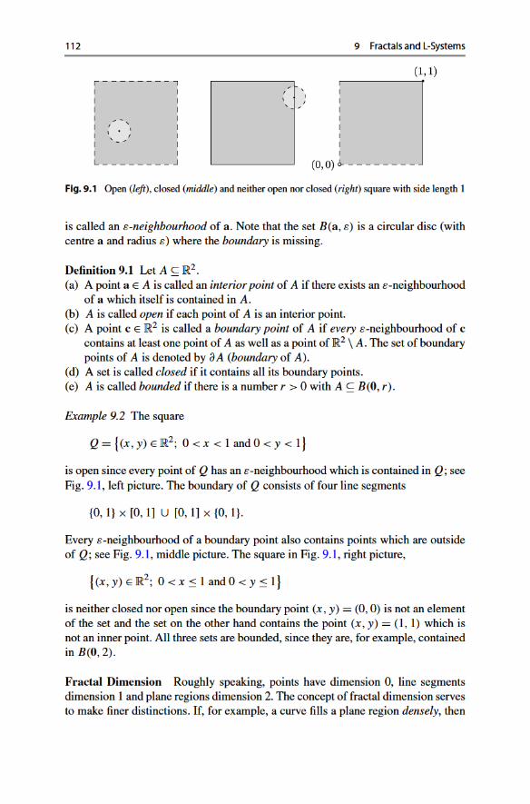
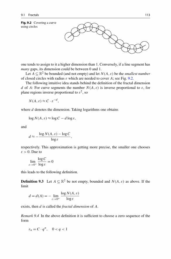
9.1 Fractals 113
Fig. 9.2 Covering a curveusing circles
one tends to assign to it a higher dimension than 1. Conversely, if a line segment hasmany gaps, its dimension could be between 0 and 1.
Let A ⊆ R2 be bounded (and not empty) and let N(A,ε) be the smallest number
of closed circles with radius ε which are needed to cover A; see Fig. 9.2.The following intuitive idea stands behind the definition of the fractal dimension
d of A: For curve segments the number N(A,ε) is inverse proportional to ε, forplane regions inverse proportional to ε2, so
N(A,ε) ≈ C · ε−d,
where d denotes the dimension. Taking logarithms one obtains
logN(A,ε) ≈ logC − d log ε,
and
d ≈ − logN(A,ε) − logC
log ε,
respectively. This approximation is getting more precise, the smaller one choosesε > 0. Due to
limε→0+
logC
log ε= 0
this leads to the following definition.
Definition 9.3 Let A ⊆ R2 be not empty, bounded and N(A,ε) as above. If the
limit
d = d(A) = − limε→0+
logN(A,ε)
log ε
exists, then d is called the fractal dimension of A.
Remark 9.4 In the above definition it is sufficient to choose a zero sequence of theform
εn = C · qn, 0 < q < 1

114 9 Fractals and L-Systems
Fig. 9.3 Raster of the plane using squares of side length ε. The boxes that have a non-emptyintersection with the fractal are coloured in grey. In the picture we have N(A,ε) = 27
Fig. 9.4 Covering of astraight line segment usingcircles
for ε. Furthermore it is not essential to use circular discs for the covering. One canjust as well use squares; see [5, Chap. 5]. Hence the number obtained by Defini-tion 9.3 is also called the box-dimension of A.
Experimentally the dimension of a fractal can be determined in the followingway: For various rasters of the plane with mesh size εn one counts the number ofboxes which have a non-empty intersection with the fractal; see Fig. 9.3. Let us callthis number again N(A,εn). If one plots logN(A,εn) as a function of log εn in adouble-logarithmic diagram and fits the best line to this graph (Sect. 18.1), then
d(A) ≈ −slope of the straight line.
With this procedure one can, for example, determine the fractal dimension of thecoastline of Great Britain; see Exercise 1.
Example 9.5 The line segment
A = {(x, y) ∈ R
2; a ≤ x ≤ b, y = c}
has fractal dimension d = 1.We choose (see Fig. 9.4)
εn = (b − a) · 2−n, q = 1/2.
Due to N(A,εn) = 2n−1 the following holds:
− logN(A,εn)
log εn
= − (n − 1) log 2
log(b − a) − n log 2→ 1 as n → ∞.
Likewise, it can easily be shown that every set that consists of finitely manypoints has fractal dimension 0. Plane regions in R
2 have fractal dimension 2. Thefractal dimension is in this way a generalisation of the intuitive notion of dimension.Still, caution is advisable here as can be seen in the following example.

9.1 Fractals 115
Fig. 9.5 A set of points with box-dimension d = 12
Example 9.6 The set F = {0,1, 12 , 1
3 , 14 , . . .} displayed in Fig. 9.5 has box-dimen-
sion d = 1/2. We check this claim with the following MATLAB experiment.
Experiment 9.7 To determine the dimension of F approximately with the helpof MATLAB we take the following steps. For j = 1,2,3, . . . we split the interval[0,1] into 4j equally large subintervals, set εj = 4−j and determine the numberNj = N(F, εj ) of subintervals which have a non-empty intersection with F . Thenwe plot logNj as a function of log εj in a double-logarithmic diagram. The slope ofthe secant
dj = − logNj+1 − logNj
log εj+1 − log εj
is an approximation to d which is steadily improving with growing j . The valuesobtained by using the program mat09_1.m are given in the following table:
4j 4 16 64 256 1024 4096 16384 65536 262144 1048576dj 0.79 0.61 0.55 0.52 0.512 0.5057 0.5028 0.5014 0.5007 0.50035
Verify the given values and determine that the approximations given by Defini-tion 9.3
dj = − logNj
log εj
are much worse. Explain this behaviour.
Example 9.8 (Cantor set) We construct this set recursively using
A0 = [0,1],A1 =
[0,
1
3
]∪
[2
3,1
],
A2 =[
0,1
9
]∪
[2
9,
1
3
]∪
[2
3,
7
9
]∪
[8
9,1
],
...
One obtains An+1 from An by removing the middle third of each line segment of An;see Fig. 9.6.
The intersection of all these sets
A =∞⋂
n=0
An
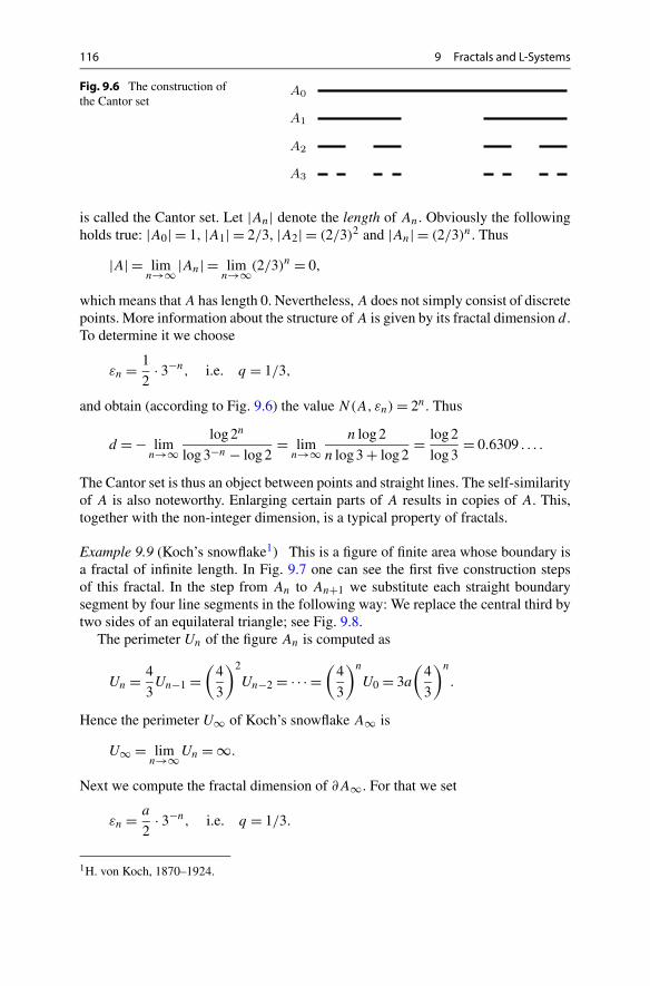
116 9 Fractals and L-Systems
Fig. 9.6 The construction ofthe Cantor set
is called the Cantor set. Let |An| denote the length of An. Obviously the followingholds true: |A0| = 1, |A1| = 2/3, |A2| = (2/3)2 and |An| = (2/3)n. Thus
|A| = limn→∞|An| = lim
n→∞(2/3)n = 0,
which means that A has length 0. Nevertheless, A does not simply consist of discretepoints. More information about the structure of A is given by its fractal dimension d .To determine it we choose
εn = 1
2· 3−n, i.e. q = 1/3,
and obtain (according to Fig. 9.6) the value N(A,εn) = 2n. Thus
d = − limn→∞
log 2n
log 3−n − log 2= lim
n→∞n log 2
n log 3 + log 2= log 2
log 3= 0.6309 . . . .
The Cantor set is thus an object between points and straight lines. The self-similarityof A is also noteworthy. Enlarging certain parts of A results in copies of A. This,together with the non-integer dimension, is a typical property of fractals.
Example 9.9 (Koch’s snowflake1) This is a figure of finite area whose boundary isa fractal of infinite length. In Fig. 9.7 one can see the first five construction stepsof this fractal. In the step from An to An+1 we substitute each straight boundarysegment by four line segments in the following way: We replace the central third bytwo sides of an equilateral triangle; see Fig. 9.8.
The perimeter Un of the figure An is computed as
Un = 4
3Un−1 =
(4
3
)2
Un−2 = · · · =(
4
3
)n
U0 = 3a
(4
3
)n
.
Hence the perimeter U∞ of Koch’s snowflake A∞ is
U∞ = limn→∞Un = ∞.
Next we compute the fractal dimension of ∂A∞. For that we set
εn = a
2· 3−n, i.e. q = 1/3.
1H. von Koch, 1870–1924.
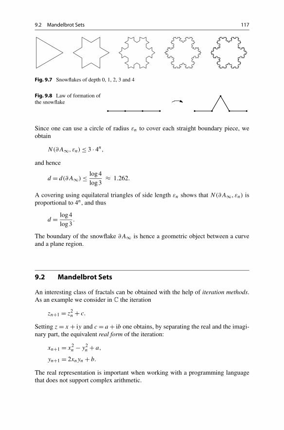
9.2 Mandelbrot Sets 117
Fig. 9.7 Snowflakes of depth 0, 1, 2, 3 and 4
Fig. 9.8 Law of formation ofthe snowflake
Since one can use a circle of radius εn to cover each straight boundary piece, weobtain
N(∂A∞, εn) ≤ 3 · 4n,
and hence
d = d(∂A∞) ≤ log 4
log 3≈ 1.262.
A covering using equilateral triangles of side length εn shows that N(∂A∞, εn) isproportional to 4n, and thus
d = log 4
log 3.
The boundary of the snowflake ∂A∞ is hence a geometric object between a curveand a plane region.
9.2 Mandelbrot Sets
An interesting class of fractals can be obtained with the help of iteration methods.As an example we consider in C the iteration
zn+1 = z2n + c.
Setting z = x + iy and c = a + ib one obtains, by separating the real and the imagi-nary part, the equivalent real form of the iteration:
xn+1 = x2n − y2
n + a,
yn+1 = 2xnyn + b.
The real representation is important when working with a programming languagethat does not support complex arithmetic.

118 9 Fractals and L-Systems
Fig. 9.9 The Mandelbrot set of the iteration zn+1 = z2n + c, z0 = 0, and enlargement of a section
First we investigate for which values of c ∈ C the iteration
zn+1 = z2n + c, z0 = 0
remains bounded. In the present case this is equivalent to |zn| → ∞ for n → ∞.The set of all c with this property is obviously not empty since it contains c = 0. Onthe other hand it is bounded since the iteration always diverges for |c| > 2 as caneasily be verified with MATLAB.
Definition 9.10 The set
M = {c ∈ C; |zn| → ∞ as n → ∞}
is called the Mandelbrot set2 of the iteration zn+1 = z2n + c, z0 = 0.
To get an impression of M we carry out a numerical experiment in MATLAB.
Experiment 9.11 To visualise the Mandelbrot set M one first chooses a raster of acertain region, for example
−2 ≤ Re c ≤ 1, −1.15 ≤ Im c ≤ 1.15.
Next for each point of the raster one carries out a large number of iterations (e.g. 80)and decides then whether the iterations remain bounded (for example |zn| ≤ 2). Ifthis is the case one colours the point in black. This way one successively obtainsa picture of M . For your experiments use the MATLAB program mat09_2.m andmodify it as required. In this way, generate in particular the pictures in Fig. 9.9 inhigh resolution.
Figure 9.9 shows as result a little apple man which has smaller apple men at-tached which finally develop into an antenna. Here one already recognises theself-similarity. If an enlargement of a certain detail on the antenna (−1.8 ≤ Re c ≤
2B. Mandelbrot, 1924–2010.

9.3 Julia Sets 119
Fig. 9.10 Julia sets of the iteration zn+1 = z2n + c for the parameter values c = −0.75 (top left),
c = 0.35 + 0.35i (top right), c = −0.03 + 0.655i (bottom left) and −0.12 + 0.74i (bottom right)
−1.72, −0.03 ≤ Im c ≤ 0.03) is made, one finds an almost perfect copy of the com-plete apple man. The Mandelbrot set is one of the most popular fractals and one ofthe most complex mathematical objects which can be visualised.
9.3 Julia Sets
Again we consider the iteration
zn+1 = z2n + c.
This time, however, we interchange the roles of z0 and c.
Definition 9.12 For a given c ∈ C, the set
Jc = {z0 ∈ C; |zn| → ∞ as n → ∞}
is called the Julia set3 of the iteration zn+1 = z2n + c.
3G. Julia, 1893–1978.

120 9 Fractals and L-Systems
The Julia set for the parameter value c hence consists of those initial values forwhich the iteration remains bounded. For some values of c the pictures of Jc aredisplayed in Fig. 9.10. Julia sets have many interesting properties, for example
Jc is connected ⇔ c ∈ M.
Thus one can alternatively define the Mandelbrot set M as
M = {c ∈ C; Jc is connected}.Furthermore, the boundary of a Julia set is self-similar and is a fractal.
Experiment 9.13 Using the MATLAB program mat09_3.m plot the Julia sets Jc inFig. 9.10 in high definition. Also try other values of c.
9.4 Newton’s Method in C
Since the arithmetic in C is an extension of that in R, many concepts of real analysiscan be transferred directly to C. For example, a function f : C → C : z �→ f (z) iscalled complex differentiable if the difference quotient
f (z + �z) − f (z)
�z
has a limit as �z → 0. This limit is again denoted by
f ′(z) = lim�z→0
f (z + �z) − f (z)
�z
and called complex derivative of f at the point z. Since differentiation in C is de-fined in the same way as differentiation in R, the same differentiation rules hold. Inparticular, any polynomial
f (z) = anzn + · · · + a1z + a0
is complex differentiable and has the derivative
f ′(z) = nanzn−1 + · · · + a1.
Like the real derivative (see Chap. 7.3), the complex derivative has an interpretationas a linear approximation
f (z) ≈ f (z0) + f ′(z0)(z − z0)
for z close to z0.

9.4 Newton’s Method in C 121
Fig. 9.11 Possible regions ofattraction of Newton’siteration for finding the rootsof z3 − 1
Let f : C → C : z �→ f (z) be a complex differentiable function with f (ζ ) = 0and f ′(ζ ) = 0. In order to compute the zero ζ of the function f , one first computesthe linear approximation starting from the initial value z0, so
z1 = z0 − f (z0)
f ′(z0).
Subsequently z1 is used as the new initial value and the procedure is iterated. In thisway, one obtains Newton’s method in C:
zn+1 = zn − f (zn)
f ′(zn).
For initial values z0 close to ζ the procedure converges (as in R) quadratically.Otherwise, however, the situation can become very complicated.
In 1983 Eckmann [9] investigated Newton’s method for the function
f (z) = z3 − 1 = (z − 1)(z2 + z + 1
).
This function has three roots in C
ζ1 = 1, ζ2,3 = −1
2± i
√3
2.
Naively one could think that the complex plane C is split into three equally largesectors where the iteration with initial values in sector S1 converges to ζ1, the onesin S2 to ζ2, etc.; see Fig. 9.11.
A numerical experiment, however, shows that it is not that way. If one coloursthe initial values according to their convergence, one obtains a very complex picture.One can prove (however, not easily imagine) that at every point where two coloursmeet, the third colour is also present. The boundaries of the regions of attraction aredominated by pincer-like motifs which reappear again and again when enlarging thescale; see Fig. 9.12. The boundaries of the regions of attraction are Julia sets. Againwe have found fractals.
Experiment 9.14 Using the MATLAB program mat09_4.m carry out an experi-ment. Ascertain yourself of the self-similarity of the appearing Julia sets by produc-ing suitable enlargements of the boundaries of the region of attraction.
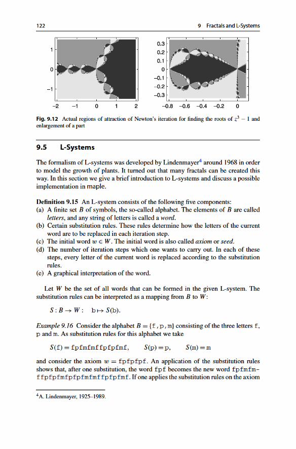

9.5 L-Systems 123
then one obtains a new word. Applying the substitution rules on that again givesa new word, and so on. Each of these words can be interpreted as a polygon byassigning the following meaning to the individual letters:
f means forward by one unit;p stands for a rotation of α radians (plus);m stands for a rotation of −α radians (minus).
Thereby 0 ≤ α ≤ π is a chosen angle. One plots the polygon by choosing an arbi-trary initial point and an arbitrary initial direction. Then one sequentially processesthe letters of the word to be displayed according to the rules above.
In maple lists and the substitution command subs lend themselves to the im-plementation of L-systems. In the example above the axiom would hence be definedby
a := [f,p,f,p,f,p,f]
and the substitution rules would be
a -> subs(f=(f,p,f,m,f,m,f,f,p,f,p,f,m,f),a).
The letters p and m do not change in the example, they are fixed points in the con-struction. For the purpose of visualisation one can use polygons in maple, given bylists of points (in the plane). These lists can be plotted easily using the commandplot.
Construction of Fractals With the graphical interpretation above and α = π/2,the axiom fpfpfpf is a square which is passed through in a counterclockwisedirection. The substitution rule converts a straight line segment into a zig-zag line.By an iterative application of the substitution rule the axiom develops into a fractal.
Experiment 9.17 Using the maple worksheet mp09_1.mws create different frac-tals. Further, try to understand the procedure fractal in detail.
Example 9.18 The substitution rule for Koch’s curve is
a -> subs(f=(f,p,f,m,m,f,p,f),a).
Depending on which axiom one uses, one can build fractal curves or snowflakesfrom this; see the maple worksheet mp09_1.mws.
Simulation of Plant Growth As a new element branchings (ramifications) areadded here. Mathematically one can describe this using two new symbols:
v stands for a ramification;e stands for the end of the branch.
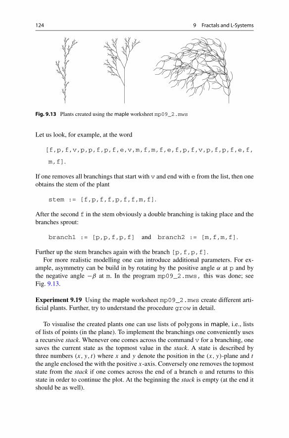
124 9 Fractals and L-Systems
Fig. 9.13 Plants created using the maple worksheet mp09_2.mws
Let us look, for example, at the word
[f,p,f,v,p,p,f,p,f,e,v,m,f,m,f,e,f,p,f,v,p,f,p,f,e,f,
m,f].
If one removes all branchings that start with v and end with e from the list, then oneobtains the stem of the plant
stem := [f,p,f,f,p,f,f,m,f].
After the second f in the stem obviously a double branching is taking place and thebranches sprout:
branch1 := [p,p,f,p,f] and branch2 := [m,f,m,f].
Further up the stem branches again with the branch [p,f,p,f].For more realistic modelling one can introduce additional parameters. For ex-
ample, asymmetry can be build in by rotating by the positive angle α at p and bythe negative angle −β at m. In the program mp09_2.mws, this was done; seeFig. 9.13.
Experiment 9.19 Using the maple worksheet mp09_2.mws create different arti-ficial plants. Further, try to understand the procedure grow in detail.
To visualise the created plants one can use lists of polygons in maple, i.e., listsof lists of points (in the plane). To implement the branchings one conveniently usesa recursive stack. Whenever one comes across the command v for a branching, onesaves the current state as the topmost value in the stack. A state is described bythree numbers (x, y, t) where x and y denote the position in the (x, y)-plane and t
the angle enclosed the with the positive x-axis. Conversely one removes the topmoststate from the stack if one comes across the end of a branch e and returns to thisstate in order to continue the plot. At the beginning the stack is empty (at the end itshould be as well).

9.6 Exercises 125
Extensions In the context of L-systems many generalisations are possible whichcan make the emerging structures more realistic. For example one could:(a) Represent the letter f by shorter segments as one moves further away from the
root of the plant. For that, one has to save the distance from the root as a furtherstate parameter in the stack.
(b) Introduce randomness by using different substitution rules for one and the sameletter and in each step choosing one at random. For example, the substitutionrules for random weeds could be such:
f -> (f,v,p,f,e,f,v,m,f,e,f) with probability 1/3;f -> (f,v,p,f,e,f) with probability 1/3;f -> (f,v,m,f,e,f) with probability 1/3.
Using random numbers, one selects the according rule in each step.
Experiment 9.20 Using the maple worksheet mp09_3.mws create random plants.Further, try to understand the implemented substitution rule in detail.
9.6 Exercises
1. Determine experimentally the fractal dimension of the coastline of Great Britain.In order to do so, take a map of Great Britain (for example a copy from an atlas)and raster the map using different mesh sizes (for example with 1/64th, 1/32th,1/16th, 1/8th and 1/4th of the North–South expansion). Count the boxes whichcontain parts of the coastline and display this number as a function of the meshsize in a double-logarithmic diagram. Fit the best line through these points anddetermine the fractal dimension in question from the slope of the straight line.
2. Using the program mat09_3.mws visualise the Julia sets of zn+1 = z2n + c for
c = −1.25 and c = 0.365 − 0.3i. Search for interesting details.3. Let f (z) = z3 − 1 with z = x + iy. Use Newton’s method to solve f (z) = 0 and
separate the real part and the imaginary part, i.e., find the functions g1 and g2with
xn+1 = g1(xn, yn),
yn+1 = g2(xn, yn).
4. Modify the procedure grow in the program mp09_2.mws by representing theletter f by shorter segments depending on how far it is away from the root. Withthe result, plot the umbel from Experiment 9.19 again.
5. Modify the program mp09_3.mws by attributing new probabilities to the ex-isting substitution rules (or invent new substitution rules). Use your modifiedprogram to plot some plants.

10Antiderivatives
The derivative of a function y = F(x) describes its local rate of change, i.e., thechange �y of the y-value with respect to the change �x of the x-value in the limit�x → 0; more precisely
f (x) = F ′(x) = lim�x→0
�y
�x= lim
�x→0
F(x + �x) − F(x)
�x.
Conversely, the question about the reconstruction of a function F from its local rateof change f leads to the notion of indefinite integrals, which comprises the totalityof all functions that have f as their derivative, the antiderivatives of f . Chapter 10addresses this notion, its properties, some basic examples and applications.
By multiplying the rate of change f (x) with the change �x one obtains an ap-proximation to the change of the values of the function of the antiderivative F in thesegment of length �x:
�y = F(x + �x) − F(x) ≈ f (x)�x.
Adding up these local changes in an interval, for instance between x = a and x = b
in steps of length �x, gives an approximation to the total change F(b)− F(a). Thelimit �x → 0 (with an appropriate increase of the number of summands) leads tothe notion of the definite integral of f in the interval [a, b], which is the subject ofChap. 11.
10.1 Indefinite Integrals
In Sect. 7.2 it was shown that the derivative of a constant is zero. The followingproposition shows that the converse is also true.
Proposition 10.1 If the function F is differentiable on (a, b) and F ′(x) = 0 for allx ∈ (a, b) then F is constant. This means that F(x) = c for a certain c ∈ R and allx ∈ (a, b).
M. Oberguggenberger, A. Ostermann, Analysis for Computer Scientists,Undergraduate Topics in Computer Science,DOI 10.1007/978-0-85729-446-3_10, © Springer-Verlag London Limited 2011
127
128 10 Antiderivatives
Proof We choose an arbitrary x0 ∈ (a, b) and set c = F(x0). If now x ∈ (a, b) then,according to the mean value theorem (Proposition 8.4),
F(x) − F(x0) = F ′(ξ)(x − x0)
for a point ξ between x and x0. Since F ′(ξ) = 0, it follows that F(x) = F(x0) = c.This holds for all x ∈ (a, b), and consequently F has to be equal to the constantfunction with value c. �
Definition 10.2 (Antiderivatives) Let f be a real-valued function on an interval(a, b). An antiderivative of f is a differentiable function F : (a, b) → R whosederivative F ′ equals f .
Example 10.3 The function F(x) = x3
3 is an antiderivative of f (x) = x2, as is
G(x) = x3
3 + 5.
Proposition 10.1 implies that antiderivatives are unique up to an additive con-stant.
Proposition 10.4 Let F and G be antiderivatives of f in (a, b). Then F(x) =G(x) + c for a certain c ∈ R and all x ∈ (a, b).
Proof Since F ′(x) − G′(x) = f (x) − f (x) = 0 for all x ∈ (a, b), an application ofProposition 10.1 gives the desired result. �
Definition 10.5 (Indefinite integrals) The indefinite integral
∫f (x)dx
denotes the totality of all antiderivatives of f .
Once a particular antiderivative F has been found, one writes accordingly∫
f (x)dx = F(x) + c.
Example 10.6 The indefinite integral of the quadratic function (Example 10.3) is∫x2 dx = x3
3 + c.
Example 10.7 (a) An application of indefinite integration to the differential equationof the vertical throw: Let w(t) denote the height (in metres [m]) at time t (in seconds[s]) of an object above ground level (w = 0). Then
w′(t) = v(t)

10.1 Indefinite Integrals 129
Fig. 10.1 Free fall: travelleddistance as function of time
is the velocity of the object (positive in upward direction) and
v′(t) = a(t)
the acceleration (positive in upward direction). In this coordinate system the gravi-tational acceleration
g = 9.81 [m/s2]acts downwards; consequently
a(t) = −g.
Velocity and distance are obtained by inverting the differentiation process:
v(t) =∫
a(t)dt + c1 = −gt + c1,
w(t) =∫
v(t)dt + c2 =∫
(−gt + c1)dt + c2 = −g
2t2 + c1t + c2,
where the constants c1, c2 are determined by the initial conditions:
c1 = v(0) initial velocity,c2 = w(0) initial height.
(b) A concrete example—free fall from a height of 100 metres. Here
w(0) = 100, v(0) = 0
and thus
w(t) = −1
29.81t2 + 100.
The travelled distance as a function of time (Fig. 10.1) is given by a parabola.The time of impact t0 is obtained from the condition w(t0) = 0, i.e.,
0 = −1
29.81t2
0 + 100, t0 = √200/9.81 ≈ 4.5 [s],

130 10 Antiderivatives
the velocity at impact is
v(t0) = −gt0 ≈ 44.3 [m/s] ≈ 160 [km/h].
10.2 Integration Formulae
It follows immediately from Definition 10.5 that indefinite integration can be seenas the inversion of differentiation. It is, however, only unique up to a constant:
(∫f (x)dx
)′= f (x),
∫g′(x)dx = g(x) + c.
With this consideration and the formulae from Sect. 7.4 one easily obtains the basicintegration formulae stated in the following table. The formulae are valid in theaccording domains.
The formulae in Table 10.1 are a direct consequence of those in Table 7.1.
Experiment 10.8 Antiderivatives can be calculated in maple using the commandint. Explanations and further integration commands can be found in the mapleworksheet mp10_1.mws. Experiment with these maple commands by applyingthem to the examples of Table 10.1 and some functions of your choice.
Experiment 10.9 Integrate the following expressions
xe−x2, e−x2
, sin(x2)
with maple.
Functions that are obtained by combining power functions, exponential functionsand trigonometric functions, as well as their inverses, are called elementary func-tions. The derivative of an elementary function is again an elementary function andcan be obtained using the rules from Chap. 7. In contrast to differentiation there is nogeneral procedure for computing indefinite integrals. Not only does the calculationof an integral often turn out to be a difficult task, but there are also many elementaryfunctions whose antiderivatives are not elementary. An algorithm to decide whethera functions has an elementary indefinite integral was first deduced by Liouville1
around 1835. This was the starting point for the field of symbolic integration. Fordetails, we refer to [7].
1J. Liouville, 1809–1882.

10.2 Integration Formulae 131
Table 10.1 Integrals of some elementary functions
f (x) xα,α �= −1 1x
ex ax
∫f (x)dx xα+1
α+1 + c log |x| + c ex + c 1loga
ax + c
f (x) sinx cosx 1√1−x2
11+x2∫
f (x)dx − cosx + c sinx + c arcsinx + c arctanx + c
Example 10.10 (Higher transcendental functions) Antiderivatives of functions thatdo not possess elementary integrals are frequently called higher transcendental func-tions. We give the following examples:Gaussian error function:
2√π
∫e−x2
dx = Erf(x) + c;
exponential integral:
∫ex
xdx = E i(x) + c;
logarithmic integral:
∫1
logxdx = �i(x) + c;
sine integral:
∫sinx
xdx = Si(x) + c;
Fresnel2 integral:
∫sin
(π
2x2
)dx = S(x) + c.
Proposition 10.11 (Rules for indefinite integration) For indefinite integration thefollowing rules hold:(a) Sum:
∫(f (x) + g(x))dx = ∫
f (x)dx + ∫g(x)dx
(b) Constant factor:∫
λf (x)dx = λ∫
f (x)dx (λ ∈ R)
(c) Integration by parts:∫
f (x)g′(x)dx = f (x)g(x) −∫
f ′(x)g(x)dx
2A.J. Fresnel, 1788–1827.
132 10 Antiderivatives
(d) Substitution:
∫f
(g(x)
)g′(x)dx =
∫f (y)dy
∣∣∣y=g(x)
.
Proof (a) and (b) are clear; (c) follows from the product rule for the derivative(Sect. 7.4)
∫f (x)g′(x)dx +
∫f ′(x)g(x)dx
=∫ (
f (x)g′(x) + f ′(x)g(x))
dx
=∫ (
f (x)g(x))′ dx = f (x)g(x) + c,
which can be rewritten as∫
f (x)g′(x)dx = f (x)g(x) −∫
f ′(x)g(x)dx.
In this formula we can drop the integration constant c, since it is already containedin the notion of indefinite integrals, which appear on both sides. Point (d) is animmediate consequence of the chain rule, according to which an antiderivative off (g(x))g′(x) is given by the antiderivative of f (y) evaluated at y = g(x). �
Example 10.12 The following five examples show how the rules of Table 10.1 andProposition 10.11 can be applied.
(a)∫
dx3√
x=
∫x− 1
3 dx = x− 13 +1
− 13 + 1
+ c = 3
2x
23 + c.
(b)∫
x cosxdx = x sinx −∫
sinx dx = x sinx + cosx + c,
which follows via integration by parts:
f (x) = x, g′(x) = cosx,
f ′(x) = 1, g(x) = sinx.
(c)∫
logx dx =∫
1 · logx dx = x logx −∫
x
xdx = x logx − x + c,
via integration by parts:
f (x) = logx, g′(x) = 1,
f ′(x) = 1
x, g(x) = x.

10.3 Exercises 133
(d)∫
x sin(x2)dx =
∫1
2siny dy
∣∣y=x2 = −1
2cosy
∣∣y=x2 + c = −1
2cos
(x2) + c,
which follows from the substitution rule with y = g(x) = x2, g′(x) = 2x,f (y) = 1
2 siny.
(e)∫
tanx dx =∫
sinx
cosxdx = − log |y| ∣∣
y=cosx+ c = − log | cosx| + c,
again after substitution with y = g(x) = cosx, g′(x) = − sinx and f (y) =−1/y.
10.3 Exercises
1. An object is thrown vertically upwards from the ground with a velocity of10 [m/s]. Find its height w(t) as a function of time t , the maximum height aswell as the time of impact on the ground.Hint. Integrate w′′(t) = −g ≈ 9.81 [m/s2] twice indefinitely and determine theintegration constants from the initial conditions w(0) = 0,w′(0) = 10.
2. Compute the following indefinite integrals by hand and with maple:(a)
∫(x + 3x2 + 5x4 + 7x6)dx
(b)∫ dx√
x
(c)∫
xe−x2dx (substitution)
(d)∫
xex dx (integration by parts).3. Compute the indefinite integrals
(a)∫
cos2 x dx
(b)∫ √
1 − x2 dx
by hand and check the results using maple.
Hints. For (a) use the identity cos2 x = 12 (1 + cos 2x); for (b) use the substitution
y = g(x) = arcsinx, f (y) = 1 − sin2 y.
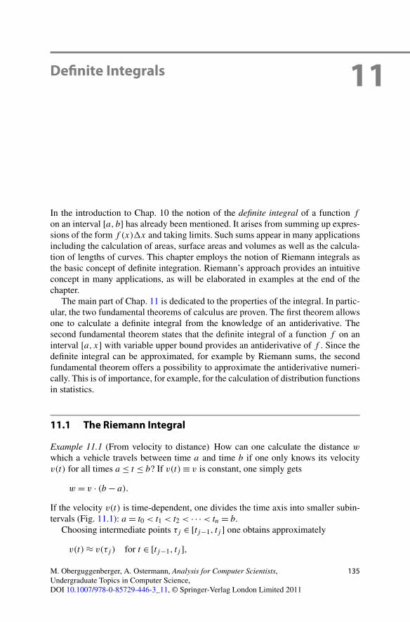
11Definite Integrals
In the introduction to Chap. 10 the notion of the definite integral of a function f
on an interval [a, b] has already been mentioned. It arises from summing up expres-sions of the form f (x)�x and taking limits. Such sums appear in many applicationsincluding the calculation of areas, surface areas and volumes as well as the calcula-tion of lengths of curves. This chapter employs the notion of Riemann integrals asthe basic concept of definite integration. Riemann’s approach provides an intuitiveconcept in many applications, as will be elaborated in examples at the end of thechapter.
The main part of Chap. 11 is dedicated to the properties of the integral. In partic-ular, the two fundamental theorems of calculus are proven. The first theorem allowsone to calculate a definite integral from the knowledge of an antiderivative. Thesecond fundamental theorem states that the definite integral of a function f on aninterval [a, x] with variable upper bound provides an antiderivative of f . Since thedefinite integral can be approximated, for example by Riemann sums, the secondfundamental theorem offers a possibility to approximate the antiderivative numeri-cally. This is of importance, for example, for the calculation of distribution functionsin statistics.
11.1 The Riemann Integral
Example 11.1 (From velocity to distance) How can one calculate the distance w
which a vehicle travels between time a and time b if one only knows its velocityv(t) for all times a ≤ t ≤ b? If v(t) ≡ v is constant, one simply gets
w = v · (b − a).
If the velocity v(t) is time-dependent, one divides the time axis into smaller subin-tervals (Fig. 11.1): a = t0 < t1 < t2 < · · · < tn = b.
Choosing intermediate points τj ∈ [tj−1, tj ] one obtains approximately
v(t) ≈ v(τj ) for t ∈ [tj−1, tj ],M. Oberguggenberger, A. Ostermann, Analysis for Computer Scientists,Undergraduate Topics in Computer Science,DOI 10.1007/978-0-85729-446-3_11, © Springer-Verlag London Limited 2011
135
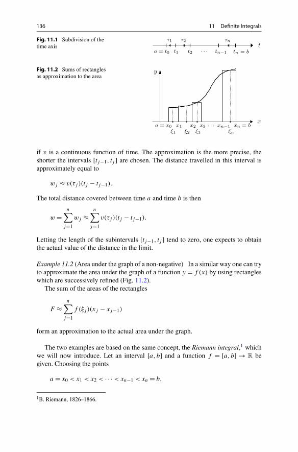
136 11 Definite Integrals
Fig. 11.1 Subdivision of thetime axis
Fig. 11.2 Sums of rectanglesas approximation to the area
if v is a continuous function of time. The approximation is the more precise, theshorter the intervals [tj−1, tj ] are chosen. The distance travelled in this interval isapproximately equal to
wj ≈ v(τj )(tj − tj−1).
The total distance covered between time a and time b is then
w =n∑
j=1
wj ≈n∑
j=1
v(τj )(tj − tj−1).
Letting the length of the subintervals [tj−1, tj ] tend to zero, one expects to obtainthe actual value of the distance in the limit.
Example 11.2 (Area under the graph of a non-negative) In a similar way one can tryto approximate the area under the graph of a function y = f (x) by using rectangleswhich are successively refined (Fig. 11.2).
The sum of the areas of the rectangles
F ≈n∑
j=1
f (ξj )(xj − xj−1)
form an approximation to the actual area under the graph.
The two examples are based on the same concept, the Riemann integral,1 whichwe will now introduce. Let an interval [a, b] and a function f = [a, b] → R begiven. Choosing the points
a = x0 < x1 < x2 < · · · < xn−1 < xn = b,
1B. Riemann, 1826–1866.

11.1 The Riemann Integral 137
the intervals [x0, x1], [x1, x2], . . . , [xn−1, xn] form a partition Z of the interval[a, b]. We denote the length of the largest subinterval by Φ(Z), i.e.,
Φ(Z) = maxj=1,...,n
|xj − xj−1|.
For arbitrarily chosen intermediate points ξj ∈ [xj−1, xj ] one calls the expression
S =n∑
j=1
f (ξj )(xj − xj−1)
a Riemann sum. In order to further specify the idea of the limiting process above,we take a sequence Z1,Z2,Z3, . . . of partitions such that Φ(ZN) → 0 as N → ∞and corresponding Riemann sums SN .
Definition 11.3 A function f is called Riemann integrable in [a, b] if, for arbitrarysequences of partitions (ZN)N≥1 with Φ(ZN) → 0, the corresponding Riemannsums (SN)N≥1 tend to the same limit I (f ), independently of the choice of the in-termediate points. This limit
I (f ) =∫ b
a
f (x)dx
is called the definite integral of f on [a, b].
The intuitive approach in the introductory Examples 11.1 and 11.2 can now bemade precise. If the respective functions f and v are Riemann integrable, then theintegral
F =∫ b
a
f (x)dx
represents the area between the x-axis and the graph, and
w =∫ b
a
v(t)dt
gives the total distance covered.
Experiment 11.4 Open the M-file mat11_1.m, study the given explanations andexperiment with randomly chosen Riemann sums for the function f (x) = 3x2 inthe interval [0,1]. What happens if you take more and more partition points n?
Experiment 11.5 Open the applet Riemann sums and study the effects of changingthe partition. In particular, vary the maximum length of the subintervals and thechoice of intermediate points. How does the sign of the function influence the result?

138 11 Definite Integrals
The following examples illustrate the notion of Riemann integrability.
Example 11.6 (a) Let f (x) = c = constant. Then the area under the graph of thefunction is the area of the rectangle c(b − a). On the other hand, any Riemann sumis of the form
f (ξ1)(x1 − x0) + f (ξ2)(x2 − x1) + · · · + f (ξn)(xn − xn−1)
= c(x1 − x0 + x2 − x1 + · · · + xn − xn−1)
= c(xn − x0) = c(b − a).
All Riemann sums are equal and thus, as expected,
∫ b
a
c dx = c(b − a).
(b) Let f (x) = 1x
for x ∈ (0,1], f (0) = 0. This function is not integrable in [0,1].The corresponding Riemann sums are of the form
1
ξ1(x1 − 0) + 1
ξ2(x2 − x1) + · · · + 1
ξn
(xn − xn−1).
By choosing ξ1 close to 0 every such Riemann sum can be made arbitrarily large,thus the limit of the Riemann sums does not exist.
(c) Dirichlet’s function2
f (x) ={
1, x ∈ Q
0, x ∈ Q
is not integrable in [0,1]. The Riemann sums are of the form
SN = f (ξ1)(x1 − x0) + · · · + f (ξn)(xn − xn−1).
If all ξj ∈ Q then SN = 1. If one takes all ξj ∈ Q then SN = 0, thus the limit dependson the choice of intermediate points ξj .
Remark 11.7 Riemann integrable functions f : [a, b] → R are necessarily bounded.This fact can easily be shown by generalising the argument in Example 11.6 (b).
The most important criteria for Riemann integrability are outlined in the follow-ing proposition. Its proof is simple, however, requires a few technical considera-tions about refining partitions. For details, we refer to the literature, for instance[4, Chap. 5.1].
2P.G.L. Dirichlet, 1805–1859.

11.1 The Riemann Integral 139
Fig. 11.3 A piecewisecontinuous function
Proposition 11.8 (a) Every function which is bounded and monotonically increas-ing (monotonically decreasing) on an interval [a, b] is Riemann integrable.
(b) Every piecewise continuous function on an interval [a, b] is Riemann inte-grable.
A function is called piecewise continuous if it is continuous except for a finitenumber of points. At these points, the graph may have jumps but is required to haveleft- and right-hand limits (Fig. 11.3).
Remark 11.9 By taking equidistant grid points a = x0 < x1 < · · · < xn−1 < xn = b
for the partition, i.e.,
xj − xj−1 =: �x = b − a
n,
the Riemann sums can be written as
SN =n∑
j=1
f (ξj )�x.
The transition �x → 0 with simultaneous increase of the number of summandssuggests the notation
∫ b
a
f (x)dx.
Originally it was introduced by Leibniz3 with the interpretation as an infinite sum ofinfinitely small rectangles of width dx. After centuries of dispute, this interpretationcan be rigorously justified today within the framework of nonstandard analysis (seefor instance [25]).
Note that the integration variable x in the definite integral is a bound variableand can be replaced by any other letter:
∫ b
a
f (x)dx =∫ b
a
f (t)dt =∫ b
a
f (ξ)dξ = · · · .
3G. Leibniz, 1646–1716.

140 11 Definite Integrals
This can be used with advantage in order to avoid possible confusion with otherbound variables.
Proposition 11.10 (Properties of the definite integral) In the following, let a < b
and f,g be Riemann integrable on [a, b].(a) Positivity:
f ≥ 0 in [a, b] ⇒∫ b
a
f (x)dx ≥ 0,
f ≤ 0 in [a, b] ⇒∫ b
a
f (x)dx ≤ 0.
(b) Monotonicity:
f ≤ g in [a, b] ⇒∫ b
a
f (x)dx ≤∫ b
a
g(x)dx.
In particular, with
m = infx∈[a,b]f (x), M = sup
x∈[a,b]f (x),
the following inequality holds:
m(b − a) ≤∫ b
a
f (x)dx ≤ M(b − a).
(c) Sum and constant factor (linearity):
∫ b
a
(f (x) + g(x)
)dx =
∫ b
a
f (x)dx +∫ b
a
g(x)dx
∫ b
a
λf (x)dx = λ
∫ b
a
f (x)dx (λ ∈ R).
(d) Partition of the integration domain: Let a < b < c and f be integrable in [a, c],then
∫ b
a
f (x)dx +∫ c
b
f (x)dx =∫ c
a
f (x)dx.
If one defines
∫ a
a
f (x)dx = 0,
∫ a
b
f (x)dx = −∫ b
a
f (x)dx,
then one obtains the validity of the sum formula even for arbitrary a, b, c ∈ R iff is integrable on the respective intervals.

11.2 Fundamental Theorems of Calculus 141
Proof All justifications are easily obtained by considering the corresponding Rie-mann sums. �
Item (a) from Proposition 11.10 shows that the interpretation of the integral asthe area under the graph is only appropriate if f ≥ 0. On the other hand, the in-terpretation of the integral of a velocity as distance travelled is also meaningful fornegative velocities (change of direction). Item (d) is especially important for the in-tegration of piecewise continuous functions (see Fig. 11.3): the integral is obtainedas the sum of the single integrals.
11.2 Fundamental Theorems of Calculus
For a Riemann integrable function f we define a new function
F(x) =∫ x
a
f (t)dt.
It is obtained by considering the upper boundary of the integration domain as vari-able.
Remark 11.11 For positive f , the value F(x) is the area under the graph of thefunction in the interval [a, x]; see Fig. 11.4.
Experiment 11.12 In maths online go to Integration in the gallery, open the appletIntuitively understanding the integral and observe the shape of the integrals F(x)
for various integrands f .
Proposition 11.13 (Fundamental theorems of calculus) Let f be continuous in[a, b]. Then the following assertions hold.(a) First fundamental theorem: If G is an antiderivative of f , then
∫ b
a
f (x)dx = G(b) − G(a).
(b) Second fundamental theorem: The function
F(x) =∫ x
a
f (t)dt
is an antiderivative of f , that is, F is differentiable and F ′(x) = f (x).
Proof In the first step we prove the second fundamental theorem. For that letx ∈ (a, b), h > 0 and x + h ∈ (a, b). According to Proposition 6.15 the functionf has a minimum and a maximum in the interval [x, x + h]:
m(h) = mint∈[x,x+h]f (t), M(h) = max
t∈[x,x+h]f (t).


11.3 Applications of the Definite Integral 143
(c)∫ 1
0x sin
(x2)dx = −1
2cos
(x2)∣∣∣∣
x=1
x=0= −1
2cos 1−
(− 1
2cos 0
)= −1
2cos 1+ 1
2
(see Example 10.12).
Remark 11.15 In maple the integration of expressions and functions is carried outusing the command int, which requires the analytic expression and the domain asarguments, for instance
int(x^2, x = 1..3);
Applications of the Second Fundamental Theorem Usually, such applicationsare of theoretical nature, like the description of the relation between travelled dis-tance and velocity,
w(t) = w(0) +∫ t
0v(s)ds, w′(t) = v(t),
where w(t) denotes the travelled distance from 0 to time t and v(t) is the instanta-neous velocity. Other applications arise in numerical analysis, for instance
∫ x
0e−y2
dy is an antiderivative of e−x2.
The value of such an integral can be approximately calculated using Taylor poly-nomials (see Application 12.18) or numerical integration methods (see Sect. 13.1).This is of particular interest if the antiderivative is not an elementary function, as isthe case for the Gaussian error function from Example 10.10.
11.3 Applications of the Definite Integral
We now turn to further applications of the definite integral, which confirm the mod-elling power of the notion of the Riemann integral.
The Volume of a Solid of Revolution Assume first that for a three-dimensionalsolid (possibly after choosing an appropriate Cartesian coordinate system) the cross-sectional area A = A(x) is known for every x ∈ [a, b]; see Fig. 11.5. The volume ofa thin slice of thickness �x is approximately equal to A(x)�x. Writing down theRiemann sums and taking limits, one obtains for the volume V of the solid
V =∫ b
a
A(x)dx.
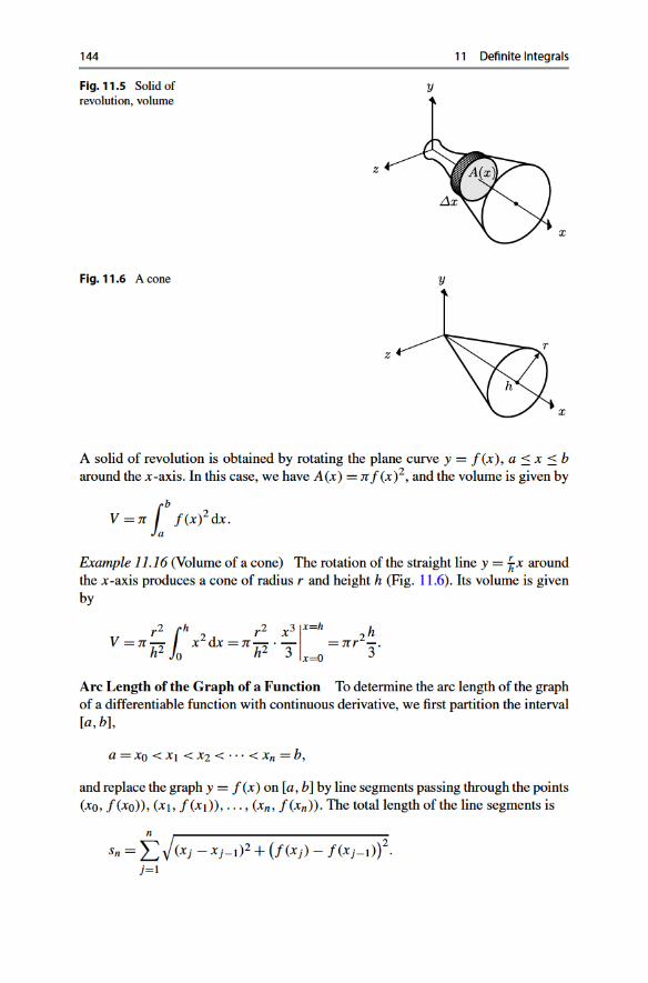

11.3 Applications of the Definite Integral 145
Fig. 11.7 The arc length of agraph
It is simply given by the sum of the lengths of the individual segments (Fig. 11.7).According to the mean value theorem (Proposition 8.4), we have
sn =n∑
j=1
√(xj − xj−1)2 + f ′(ξj )2(xj − xj−1)2
=n∑
j=1
√1 + f ′(ξj )2 (xj − xj−1),
with certain points ξj ∈ [xj−1, xj ]. The sums sn are easily identified as Riemannsums. Their limit is thus given by
s =∫ b
a
√1 + f ′(x)2 dx.
Lateral Surface Area of a Solid of Revolution The lateral surface of a solid ofrevolution is obtained by rotating the curve y = f (x), a ≤ x ≤ b around the x-axis.
In order to determine its area, we split the solid into small slices of thickness�x. Each of these slices is approximately a truncated cone with generator of length�s and mean radius f (x); see Fig. 11.8. According to Exercise 11 of Chap. 3 thelateral surface area of this truncated cone is equal to 2πf (x)�s. According to whathas been said previously, �s ≈ √
1 + f ′(x)2�x, and thus the lateral surface area ofa small slice is approximately equal to
2πf (x)
√1 + f ′(x)2�x.
Writing down the Riemann sums and taking limits, one obtains
M = 2π
∫ b
a
f (x)
√1 + f ′(x)2 dx
for the lateral surface area.
Example 11.17 (Surface area of a sphere) The surface of a sphere of radius r isgenerated by rotation of the graph f (x) = √
r2 − x2,−r ≤ x ≤ r . One obtains
M = 2π
∫ r
−r
√r2 − x2 r√
r2 − x2dx = 4πr2.
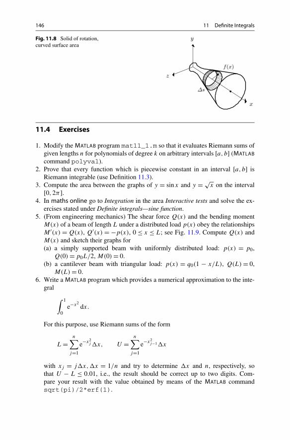
146 11 Definite Integrals
Fig. 11.8 Solid of rotation,curved surface area
11.4 Exercises
1. Modify the MATLAB program mat11_1.m so that it evaluates Riemann sums ofgiven lengths n for polynomials of degree k on arbitrary intervals [a, b] (MATLABcommand polyval).
2. Prove that every function which is piecewise constant in an interval [a, b] isRiemann integrable (use Definition 11.3).
3. Compute the area between the graphs of y = sinx and y = √x on the interval
[0,2π].4. In maths online go to Integration in the area Interactive tests and solve the ex-
ercises stated under Definite integrals—sine function.5. (From engineering mechanics) The shear force Q(x) and the bending moment
M(x) of a beam of length L under a distributed load p(x) obey the relationshipsM ′(x) = Q(x), Q′(x) = −p(x), 0 ≤ x ≤ L; see Fig. 11.9. Compute Q(x) andM(x) and sketch their graphs for(a) a simply supported beam with uniformly distributed load: p(x) = p0,
Q(0) = p0L/2, M(0) = 0.(b) a cantilever beam with triangular load: p(x) = q0(1 − x/L), Q(L) = 0,
M(L) = 0.6. Write a MATLAB program which provides a numerical approximation to the inte-
gral
∫ 1
0e−x2
dx.
For this purpose, use Riemann sums of the form
L =n∑
j=1
e−x2j �x, U =
n∑j=1
e−x2j−1�x
with xj = j�x,�x = 1/n and try to determine �x and n, respectively, sothat U − L ≤ 0.01, i.e., the result should be correct up to two digits. Com-pare your result with the value obtained by means of the MATLAB commandsqrt(pi)/2*erf(1).

11.4 Exercises 147
Fig. 11.9 Simply supported beam with uniformly distributed load, cantilever beam with triangularload
Additional task: Extend your program so that it allows one to compute∫ a
0 e−x2dx
for arbitrary a > 0.7. Show that the error of approximating the integral in Exercise 6 either by L or U
is at most U − L. Use the applet Integration to visualise this fact.Hint. Verify the inequality
L ≤∫ 1
0e−x2
dx ≤ U.
Thus, L and U are lower and upper sums, respectively.8. Rotation of the parabola y = 2
√x, 0 ≤ x ≤ 1 around the x-axis produces a
paraboloid. Sketch it and compute its volume and its lateral surface area.

12Taylor Series
Approximations of complicated functions by simpler functions play a vital part inapplied mathematics. Starting with the concept of linear approximation we discussthe approximation of a function by Taylor polynomials and by Taylor series in thischapter. As important applications we will use Taylor series to compute limits offunctions and to analyse various approximation formulae.
12.1 Taylor’s Formula
In this section we consider the approximation of sufficiently smooth functions bypolynomials as well as applications of these approximations. We have already seenan approximation formula in Chap. 7: Let f be a function that is differentiable at a.Then
f (x) ≈ g(x) = f (a) + f ′(a) · (x − a),
for all x close to a. The linear approximation g is a polynomial of degree 1 in x, itsgraph is just the tangent to f at a. We now want to generalise this approximationresult.
Proposition 12.1 (Taylor’s formula1) Let I ⊆ R be an open interval and f : I → R
an (n + 1)-times continuously differentiable function (i.e., the derivative of order(n + 1) of f exists and is continuous). Then, for all x, a ∈ I ,
f (x) = f (a) + f ′(a) · (x − a) + f ′′(a)
2! (x − a)2 + · · ·
+ f (n)(a)
n! (x − a)n + Rn+1(x, a)
1B. Taylor, 1685–1731.
M. Oberguggenberger, A. Ostermann, Analysis for Computer Scientists,Undergraduate Topics in Computer Science,DOI 10.1007/978-0-85729-446-3_12, © Springer-Verlag London Limited 2011
149

150 12 Taylor Series
with the remainder term (in integral form)
Rn+1(x, a) = 1
n!∫ x
a
(x − t)nf (n+1)(t)dt.
Alternatively the remainder term can be expressed by
Rn+1(x, a) = f (n+1)(ξ)
(n + 1)! (x − a)n+1,
where ξ is a point between a and x (Lagrange’s2 form of the remainder term).
Proof According to the fundamental theorem of calculus, we have
∫ x
a
f ′(t)dt = f (x) − f (a),
and thus
f (x) = f (a) +∫ x
a
f ′(t)dt.
We apply integration by parts to this formula. Due to
∫ x
a
u′(t)v(t)dt = u(t)v(t)∣∣xa
−∫ x
a
u(t)v′(t)dt
with u(t) = t − x and v(t) = f ′(t) we get
f (x) = f (a) + (t − x)f ′(t)∣∣xa
−∫ x
a
(t − x)f ′′(t)dt
= f (a) + f ′(a) · (x − a) +∫ x
a
(x − t)f ′′(t)dt.
A further integration by parts yields
∫ x
a
(x − t)f ′′(t)dt = − (x − t)2
2f ′′(t)
∣∣xa
+∫ x
a
(x − t)2
2f ′′′(t)dt
= f ′′(a)
2(x − a)2 + 1
2
∫ x
a
(x − t)2f ′′′(t)dt,
and one recognises that repeated integration by parts leads to the desired formula(with the remainder term in integral form). The other representation of the remainderterm follows from the mean value theorem for integrals [4, Chap. 5, Theorem 5.4]. �
2J.L. Lagrange, 1736–1813.

12.1 Taylor’s Formula 151
Example 12.2 (Important special case) If one sets x = a + h and replaces a by x inTaylor’s formula, then one obtains
f (x + h) = f (x) + hf ′(x) + h2
2f ′′(x) + · · ·+ hn
n! f(n)(x) + hn+1
(n + 1)!f(n+1)(ξ)
with a point ξ between x and x + h. For small h this formula describes how thefunction f behaves near x.
Remark 12.3 Often one does not know the remainder term
Rn+1(x, a) = f (n+1)(ξ)
(n + 1)! (x − a)n+1
explicitly since ξ is unknown in general. Let M be the supremum of |f (n+1)| in theconsidered interval around a. For x in this interval we obtain the bound
∣∣Rn+1(x, a)∣∣ ≤ M
(n + 1)! (x − a)n+1.
The remainder term is thus bounded by a constant times hn+1, where h = x − a. Inthis situation, one writes for short
Rn+1(a + h,a) = O(hn+1)
as h → 0 and calls the remainder a term of order n + 1. This notation is also usedby maple.
Definition 12.4 The polynomial
Tn(x, a) = f (a) + f ′(a) · (x − a) + · · · + f (n)(a)
n! (x − a)n
is called nth Taylor polynomial of f around the point of expansion a.
The graphs of the functions y = Tn(x, a) and y = f (x) both pass through thepoint (a, f (a)). Their tangents in this point have the same slope T ′
n(x, a) = f ′(a)
and the graphs have the same curvature (due to T ′′n (x, a) = f ′′(a); see Chap. 14). It
depends on the size of the remainder term how well the Taylor polynomial approxi-mates the function.
Example 12.5 (Taylor polynomial of the exponential function) Let f (x) = ex anda = 0. Due to (ex)′ = ex we have f (k)(0) = e0 = 1 for all k ≥ 0 and hence
ex = 1 + x + x2
2+ · · · + xn
n! + eξ
(n + 1)!xn+1,
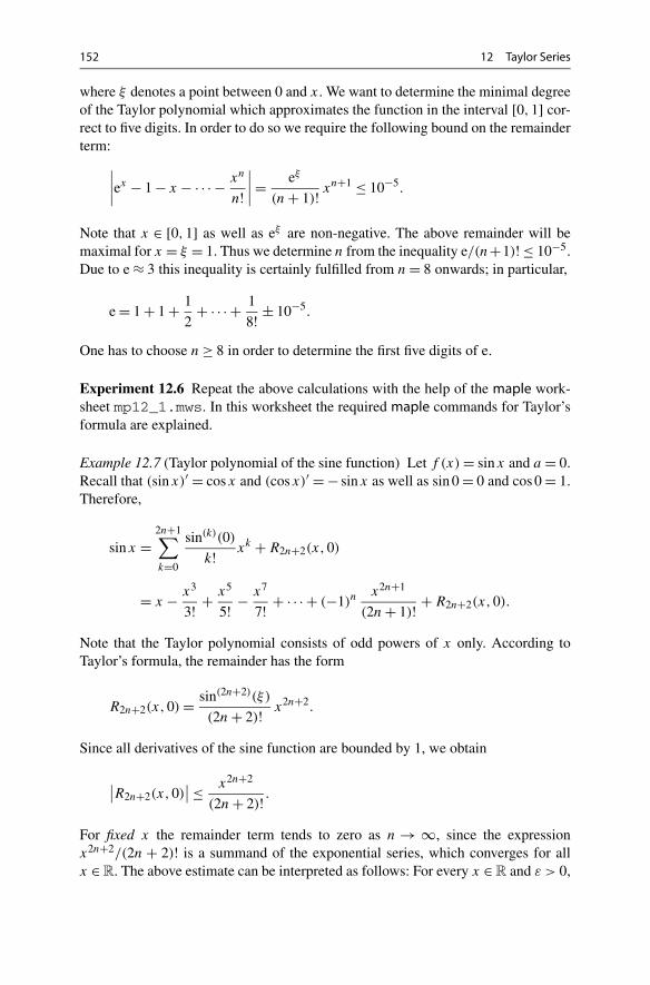
152 12 Taylor Series
where ξ denotes a point between 0 and x. We want to determine the minimal degreeof the Taylor polynomial which approximates the function in the interval [0,1] cor-rect to five digits. In order to do so we require the following bound on the remainderterm:
∣∣∣∣ex − 1 − x − · · · − xn
n!∣∣∣∣ = eξ
(n + 1)! xn+1 ≤ 10−5.
Note that x ∈ [0,1] as well as eξ are non-negative. The above remainder will bemaximal for x = ξ = 1. Thus we determine n from the inequality e/(n+1)! ≤ 10−5.Due to e ≈ 3 this inequality is certainly fulfilled from n = 8 onwards; in particular,
e = 1 + 1 + 1
2+ · · · + 1
8! ± 10−5.
One has to choose n ≥ 8 in order to determine the first five digits of e.
Experiment 12.6 Repeat the above calculations with the help of the maple work-sheet mp12_1.mws. In this worksheet the required maple commands for Taylor’sformula are explained.
Example 12.7 (Taylor polynomial of the sine function) Let f (x) = sinx and a = 0.Recall that (sinx)′ = cosx and (cosx)′ = − sinx as well as sin 0 = 0 and cos 0 = 1.Therefore,
sinx =2n+1∑k=0
sin(k)(0)
k! xk + R2n+2(x,0)
= x − x3
3! + x5
5! − x7
7! + · · · + (−1)nx2n+1
(2n + 1)! + R2n+2(x,0).
Note that the Taylor polynomial consists of odd powers of x only. According toTaylor’s formula, the remainder has the form
R2n+2(x,0) = sin(2n+2)(ξ)
(2n + 2)! x2n+2.
Since all derivatives of the sine function are bounded by 1, we obtain
∣∣R2n+2(x,0)∣∣ ≤ x2n+2
(2n + 2)! .
For fixed x the remainder term tends to zero as n → ∞, since the expressionx2n+2/(2n + 2)! is a summand of the exponential series, which converges for allx ∈ R. The above estimate can be interpreted as follows: For every x ∈ R and ε > 0,
12.2 Taylor’s Theorem 153
there exists an integer N ∈ N such that the difference of the sine function and its nthTaylor polynomial is small; more precisely,
∣∣sin t − Tn(t,0)∣∣ ≤ ε
for all n ≥ N and t ∈ [−x, x].
Experiment 12.8 Using the maple worksheet mp12_2.mws compute the Taylorpolynomials of sinx around the point 0 and determine the accuracy of the approx-imation (by plotting the difference to sinx). In order to achieve high accuracy forlarge x, the degree of the polynomials has to be chosen sufficiently high. Due torounding errors, however, this procedure quickly reaches its limits (unless one in-creases the number of significant digits).
Example 12.9 The fourth degree Taylor polynomial T4(x,0) of the function
f (x) ={
xex−1 x = 0,
1 x = 0,
is given by
T4(x,0) = 1 − x
2+ 1
12x2 − 1
720x4.
Experiment 12.10 The maple worksheet mp12_3.mws shows that, for suffi-ciently large n, the Taylor polynomial of degree n gives a good approximation tothe function from Example 12.9 on closed subintervals of (−2π,2π). For x ≥ 2π
(as well as for x ≤ −2π ) the Taylor polynomial is, however, useless.
12.2 Taylor’s Theorem
The last example gives rise to the question for which points the Taylor polynomialconverges to the function as n → ∞.
Definition 12.11 Let I ⊆ R be an open interval and let f : I → R have arbitrarilymany derivatives. Given a ∈ I , the series
T (x, a,f ) =∞∑
k=0
f (k)(a)
k! (x − a)k
is called Taylor series of f around the point a.

154 12 Taylor Series
Proposition 12.12 (Taylor’s theorem) Let f : I → R be a function with arbitrarilymany derivatives and let T (x, a,f ) be its Taylor series around the point a. Then thefunction and its Taylor series coincide at x ∈ I , i.e.,
f (x) =∞∑
k=0
f (k)(a)
k! (x − a)k,
if and only if the remainder term
Rn(x, a) = f (n)(ξ)
n! (x − a)n
tends to 0 as n → ∞.
Proof According to Taylor’s formula (Proposition 12.1),
f (x) − Tn(x, a) = Rn+1(x, a)
and hence
f (x) = limn→∞Tn(x, a) = T (x, a,f ) ⇔ lim
n→∞Rn(x, a) = 0,
which was to be shown. �
Example 12.13 Let f (x) = sinx and a = 0. Due to Rn(x,0) = sin(n)(ξ)n! xn we have
∣∣Rn(x,0)∣∣ ≤ |x|n
n! → 0
for x fixed and n → ∞. Hence for all x ∈ R
sinx =∞∑
k=0
(−1)kx2k+1
(2k + 1)! = x − x3
3! + x5
5! − x7
7! + x9
9! ∓ · · · .
12.3 Applications of Taylor’s Formula
To complete this chapter we discuss a few important applications of Taylor’s for-mula.
Application 12.14 (Extremum test) Let the function f : I → R be n-times contin-uously differentiable in the interval I and assume that
f ′(a) = f ′′(a) = · · · = f (n−1)(a) = 0 and f (n)(a) = 0.
Then the following assertions hold:
12.3 Applications of Taylor’s Formula 155
(a) The function f has an extremum at a if and only if n is even.(b) If n is even and f (n)(a) > 0, then a is a local minimum of f .
If n is even and f (n)(a) < 0, then a is a local maximum of f .
Proof Due to Taylor’s formula, we have
f (x) − f (a) = f (n)(ξ)
n! (x − a)n, x ∈ I.
If x is close to a, f (n)(ξ) and f (n)(a) have the same signs (since f (n) is continuous).For n odd the right-hand side changes its sign at x = a because of the term (x −a)n.Hence an extremum can only occur for n even. If now n is even and f (n)(a) > 0,then f (x) > f (a) for all x close to a with x = a. Thus a is a local minimum. �
Example 12.15 The polynomial f (x) = 6+4x +6x2 +4x3 +x4 has the derivatives
f ′(−1) = f ′′(−1) = f ′′′(−1) = 0, f (4)(−1) = 24
at the point x = −1. Hence x = −1 is a local minimum of f .
Application 12.16 (Computation of limits of functions) As an example, we inves-tigate the function
g(x) = x2 log(1 + x)
(1 − cosx) sinx
in the neighbourhood of x = 0. For x = 0 we obtain the undefined expression 00 . In
order to determine the limit when x tends to 0, we expand all appearing functions inTaylor polynomials around the point a = 0. Exercise 1 yields the result that cosx =1 − x2
2 + O(x4). Taylor’s formula for log(1 + x) around the point a = 0 reads
log(1 + x) = x + O(x2),
because of log 1 = 0 and log(1 + x)′|x=0 = 1. We thus obtain
g(x) = x2(x + O(x2))
(1 − 1 + x2
2 + O(x4))(x + O(x3))= x3 + O(x4)
x3
2 + O(x5)= 1 + O(x)
12 + O(x2)
and consequently limx→0 g(x) = 2.
Application 12.17 (Analysis of approximation formulae) When differentiating nu-merically in Chap. 7, we considered the symmetric difference quotient
f ′′(x) ≈ f (x + h) − 2f (x) + f (x − h)
h2

156 12 Taylor Series
as an approximation to the second derivative f ′′(x). We are now in the position toinvestigate the accuracy of this formula. From
f (x + h) = f (x) + hf ′(x) + h2
2f ′′(x) + h3
6f ′′′(x) + O
(h4),
f (x − h) = f (x) − hf ′(x) + h2
2f ′′(x) − h3
6f ′′′(x) + O
(h4),
we infer that
f (x + h) + f (x − h) = 2f (x) + h2f ′′(x) + O(h4)
and hence
f (x + h) − 2f (x) + f (x − h)
h2= f ′′(x) + O
(h2).
One calls this formula second-order accurate. If one reduces h by the factor λ, thenthe error reduces by the factor λ2, as long as rounding errors do not play a decisiverole.
Application 12.18 (Integration of functions that do not possess elementary inte-grals) As already mentioned in Sect. 10.2 there are functions whose antideriva-tives cannot be expressed as combinations of elementary functions. For example,the function f (x) = e−x2
does not have an elementary integral. In order to computethe definite integral
∫ 1
0e−x2
dx,
we approximate e−x2by the Taylor polynomial of degree 8
e−x2 ≈ 1 − x2 + x4
2− x6
6+ x8
24
and approximate the integral sought after by
∫ 1
0
(1 − x2 + x4
2− x6
6+ x8
24
)dx = 5651
7560.
The error of this approximation is 6.63 · 10−4. For more precise results one takes aTaylor polynomial of a higher degree.
Experiment 12.19 Using the maple worksheet mp12_4.mws repeat the calcula-tions from Application 12.18. Subsequently modify the program such that you canintegrate g(x) = cos(x2) with it.

12.4 Exercises 157
12.4 Exercises
1. Compute the Taylor polynomials of degree 0,1,2,3 and 4 of the function g(x) =cosx around the point of expansion a = 0. For which x ∈ R does the Taylor seriesof cosx converge?
2. Compute the Taylor polynomials of degree 1,3 and 5 of the function sinx aroundthe point of expansion a = 9π . Further, compute the Taylor polynomial of de-gree 39 with maple and plot the graph together with the graph of the function inthe interval [0,18π]. In order to better be able to distinguish the two graphs youshould plot them in different colours.
3. Compute the Taylor polynomials of degree 1,2 and 3 of the function f (t) =√1 + t around the point of expansion a = 0. Furthermore, compute the Taylor
polynomial of degree 10 with maple.4. Compute the following limits using Taylor series expansion:
limx→0
x sinx − x2
2 cosx − 2 + x2, lim
x→0
e2x − 1 − 2x
sin2 x,
limx→0
e−x2 − 1
sin2(3x), lim
x→0
x2(log(1 − 2x))2
1 − cos(x2).
Verify your results with maple.5. For the approximate evaluation of the integral
∫ 1
0
sin(t2)
tdt
replace the integrand by its Taylor polynomial of degree 9 and integrate thispolynomial. Verify your result with maple.
6. Prove the formula
eiϕ = cosϕ + i sinϕ
by substituting the value iϕ for x into the series of the exponential function
ex =∞∑
k=0
xk
k!
and separating real and imaginary parts.
13Numerical Integration
The fundamental theorem of calculus suggests the following approach to the calcu-lation of definite integrals: one determines an antiderivative F of the integrand f
and computes from that the value of the integral
∫ b
a
f (x)dx = F(b) − F(a).
In practice, however, it is difficult and often even impossible to find an antiderivativeF as a combination of elementary functions. Apart from that, antiderivatives canalso be fairly complex, as the example
∫x100 sinx dx shows. Finally, in concrete
applications the integrand is often given numerically and not by an explicit formula.In all these cases one reverts to numerical methods. In this chapter the basic conceptsof numerical integration (quadrature formulae and their order) are introduced andexplained. By means of instructive examples we analyse the achievable accuracyfor the Gaussian quadrature formulae and the required computational effort.
13.1 Quadrature Formulae
For the numerical computation of∫ b
af (x)dx we first split the interval of integration
[a, b] into subintervals with grid points a = x0 < x1 < x2 < · · · < xN−1 < xN = b;see Fig. 13.1. From the additivity of the integral (Proposition 11.10 (d)) we get
∫ b
a
f (x)dx =N−1∑j=0
∫ xj+1
xj
f (x)dx.
Hence it is sufficient to find an approximation formula for a (small) subintervalof length hj = xj+1 − xj . One example of such a formula is the trapezoidal rulethrough which the area under the graph of a function is approximated by the area of
M. Oberguggenberger, A. Ostermann, Analysis for Computer Scientists,Undergraduate Topics in Computer Science,DOI 10.1007/978-0-85729-446-3_13, © Springer-Verlag London Limited 2011
159
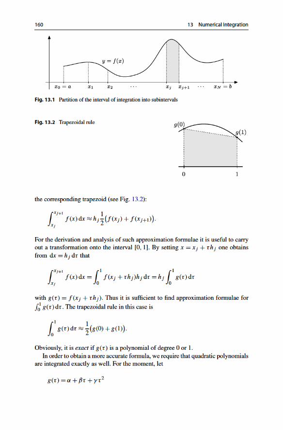
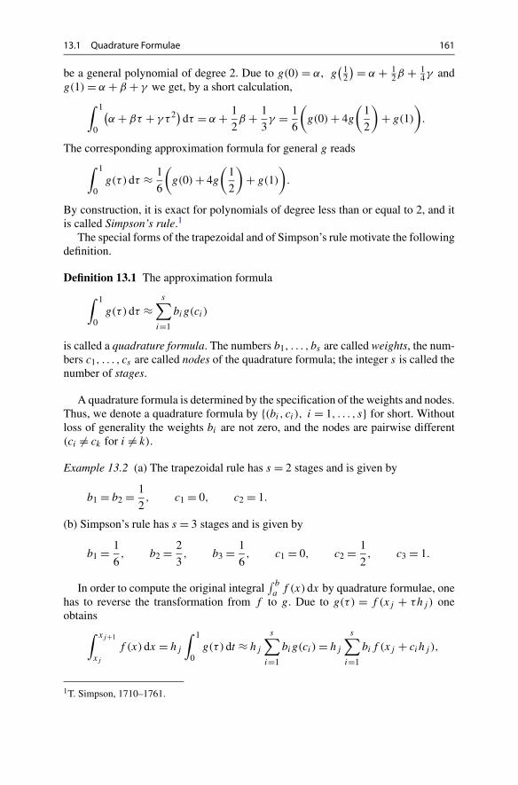
13.1 Quadrature Formulae 161
be a general polynomial of degree 2. Due to g(0) = α, g( 1
2
) = α + 12β + 1
4γ andg(1) = α + β + γ we get, by a short calculation,
∫ 1
0
(α + βτ + γ τ 2)dτ = α + 1
2β + 1
3γ = 1
6
(g(0) + 4g
(1
2
)+ g(1)
).
The corresponding approximation formula for general g reads∫ 1
0g(τ)dτ ≈ 1
6
(g(0) + 4g
(1
2
)+ g(1)
).
By construction, it is exact for polynomials of degree less than or equal to 2, and itis called Simpson’s rule.1
The special forms of the trapezoidal and of Simpson’s rule motivate the followingdefinition.
Definition 13.1 The approximation formula
∫ 1
0g(τ)dτ ≈
s∑i=1
big(ci)
is called a quadrature formula. The numbers b1, . . . , bs are called weights, the num-bers c1, . . . , cs are called nodes of the quadrature formula; the integer s is called thenumber of stages.
A quadrature formula is determined by the specification of the weights and nodes.Thus, we denote a quadrature formula by {(bi, ci), i = 1, . . . , s} for short. Withoutloss of generality the weights bi are not zero, and the nodes are pairwise different(ci �= ck for i �= k).
Example 13.2 (a) The trapezoidal rule has s = 2 stages and is given by
b1 = b2 = 1
2, c1 = 0, c2 = 1.
(b) Simpson’s rule has s = 3 stages and is given by
b1 = 1
6, b2 = 2
3, b3 = 1
6, c1 = 0, c2 = 1
2, c3 = 1.
In order to compute the original integral∫ b
af (x)dx by quadrature formulae, one
has to reverse the transformation from f to g. Due to g(τ) = f (xj + τhj ) oneobtains
∫ xj+1
xj
f (x)dx = hj
∫ 1
0g(τ)dt ≈ hj
s∑i=1
big(ci) = hj
s∑i=1
bif (xj + cihj ),
1T. Simpson, 1710–1761.
162 13 Numerical Integration
and thus we have the approximation formula
∫ b
a
f (x)dx =N−1∑j=0
∫ xj+1
xj
f (x)dx ≈N−1∑j=0
hj
s∑i=1
bif (xj + cihj ).
We now look for quadrature formulae that are as accurate as possible. Since theintegrand is typically well approximated by Taylor polynomials on small intervals,a good quadrature formula is characterised by the property that it integrates exactlyas many polynomials as possible. This idea motivates the following definition.
Definition 13.3 (Order) The quadrature formula {(bi, ci), i = 1, . . . , s} has orderp if all polynomials g of degree less or equal to p − 1 are integrated exactly by thequadrature formula, i.e.,
∫ 1
0g(τ)dτ =
s∑i=1
big(ci)
for all polynomials g of degree smaller than or equal to p − 1.
Example 13.4 (a) The trapezoidal rule has order 2.(b) Simpson’s rule has (by construction) at least order 3.
The following proposition yields an algebraic characterisation of the order ofquadrature formulae.
Proposition 13.5 A quadrature formula {(bi, ci), i = 1, . . . , s} has order p if andonly if
s∑i=1
bicq−1i = 1
qfor 1 ≤ q ≤ p.
Proof One uses the fact that a polynomial g of degree p − 1,
g(τ) = α0 + α1τ + · · · + αp−1τp−1,
is a linear combination of monomials, and that both integration and application of aquadrature formula are linear processes. Thus, it is sufficient to prove the result forthe monomials
g(τ) = τq−1, 1 ≤ q ≤ p.
The proposition now follows directly from the identity
1
q=
∫ 1
0τq−1 dτ =
s∑i=1
big(ci) =s∑
i=1
bicq−1i .
�
13.1 Quadrature Formulae 163
The conditions of the proposition
b1 + b2 + · · · + bs = 1,
b1c1 + b2c2 + · · · + bscs = 1
2,
b1c21 + b2c
22 + · · · + bsc
2s = 1
3,
...
b1cp−11 + b2c
p−12 + · · · + bsc
p−1s = 1
p
are called order conditions of order p. If s nodes c1, . . . , cs are given, then theorder conditions form a linear system of equations for the unknown weights bi . Ifthe nodes are pairwise different, then the weights can be determined uniquely fromthat. This shows that for s different nodes there always exists a unique quadratureformula of order p ≥ s.
Example 13.6 We determine once more the order of Simpson’s rule. Due to
b1 + b2 + b3 = 1
6+ 2
3+ 1
6= 1,
b1c1 + b2c2 + b3c3 = 2
3· 1
2+ 1
6= 1
2,
b1c21 + b2c
22 + b3c
23 = 2
3· 1
4+ 1
6= 1
3,
its order is at least 3 (as we already know from the construction). However, addi-tionally
b1c31 + b2c
32 + b3c
33 = 4
6· 1
8+ 1
6= 3
12= 1
4,
i.e., Simpson’s rule even has order 4.
The best quadrature formulae (high accuracy with little computational effort) arethe Gaussian quadrature formulae. For that we state the following result whose proofcan be found in [22, Chap. 10, Corollary 10.1].
Proposition 13.7 There is no quadrature formula with s stages of order p > 2s. Onthe other hand, for every s ∈ N there exists a (unique) quadrature formula of orderp = 2s. This formula is called s-stage Gaussian quadrature formula.

164 13 Numerical Integration
The Gaussian quadrature formulae for s ≤ 3 are
s = 1 : c1 = 1
2, b1 = 1, order 2 (midpoint rule);
s = 2 : c1 = 1
2−
√3
6, c2 = 1
2+
√3
6, b1 = b2 = 1
2, order 4;
s = 3 : c1 = 1
2−
√15
10, c2 = 1
2, c3 = 1
2+
√15
10,
b1 = 5
18, b2 = 8
18, b3 = 5
18, order 6.
13.2 Accuracy and Efficiency
In the following numerical experiment the accuracy of quadrature formulae will beillustrated. With the help of the Gaussian quadrature formulae of order 2, 4 and 6we compute the two integrals
∫ 3
0cosx dx = sin 3 and
∫ 1
0x5/2 dx = 2
7.
In order to do so we choose equidistant grid points
xj = a + jh, j = 0, . . . ,N
with h = (b−a)/N and N = 1,2,4,8,16, . . . ,512. Finally, we plot the costs of thecalculation as a function of the achieved accuracy in a double-logarithmic diagram.
A measure for the computational costs of a quadrature formula is the numberof required function evaluations, abbreviated by fe. For an s-stage quadrature for-mula, it is the number
fe= s · N.
The achieved accuracy err is the absolute value of the error. The according resultsare presented in Fig. 13.3. One makes the following observations:(a) The curves are straight lines (as long as one does not get into the range of round-
ing errors, like with the three-stage method in the left picture).(b) In the left picture the straight lines have slope −1/p, where p is the order of
the quadrature formula. In the right picture this is only true for the method oforder 2; the other two methods result in straight lines with slope −2/7.
(c) For given costs the formulae of higher order are more accurate.In order to understand this behaviour, we expand the integrand into a Taylor
series. On the subinterval [α,α + h] of length h we obtain
f (α + τh) =p−1∑q=0
hq
q! f(q)(α)τq + O
(hp
).

13.2 Accuracy and Efficiency 165
Fig. 13.3 Accuracy–cost-diagram of the Gaussian quadrature formulae. The crosses are the re-sults of the one-stage Gaussian method of order 2, the squares the ones of the two-stage method oforder 4 and the circles the ones of the three-stage method of order 6
Since a quadrature formula of order p integrates polynomials of degree less than orequal to p−1 exactly, the Taylor polynomial of f of degree p−1 is being integratedexactly. The error of the quadrature formula on this subinterval is proportional to thelength of the interval times the size of the remainder term of the integrand, so
h · O(hp
) = O(hp+1).
In total we have N subintervals; hence the total error of the quadrature formula is
N · O(hp+1) = Nh · O
(hp
) = (b − a) · O(hp
) = O(hp
).
Thus, we have shown that (for small h) the error err behaves like
err≈ c1 · hp.
Since, furthermore,
fe= sN = s · Nh · h−1 = s · (b − a) · h−1 = c2 · h−1
holds true, we obtain
log(fe) = log c2 − logh and log(err) ≈ log c1 + p · logh,
so altogether
log(fe) ≈ c3 − 1
p· log(err).
This explains why straight lines with slope −1/p appear in the left picture.
166 13 Numerical Integration
In the right picture we note that the second derivative of the integrand is discon-tinuous at 0. Hence the above considerations with the Taylor series are not validanymore. The quadrature formula also detects this discontinuity of the high deriva-tives and reacts with a so-called order reduction, i.e., the methods show a lowerorder (in our case p = 7/2).
Experiment 13.8 Compute the integrals
∫ 3
0
√x dx and
∫ 2
1
dx
x
using the Gaussian quadrature formulae and generate an accuracy-cost-diagram.For that purpose modify the programs mat13_1.m, mat13_2.m, mat13_3.m,mat13_4.m and mat13_5.m with which Fig. 13.3 was produced.
Commercial programs for numerical integration determine the grid points adap-tively based on automatic error estimates. The user can usually specify the desiredaccuracy. In MATLAB the routines quad.m and quadl.m serve this purpose.
13.3 Exercises
1. For the calculation of∫ 1
0 x100 sinx dx first determine an antiderivative F of theintegrand f using maple. Then evaluate F(1) − F(0) to 10, 50, 100, 200 and400 digits and explain the surprising results.
2. Determine the order of the quadrature formula given by
b1 = b4 = 1
8, b2 = b3 = 3
8,
c1 = 0, c2 = 1
3, c3 = 2
3, c4 = 1.
3. Determine the unique quadrature formula of order 3 with the nodes
c1 = 1
3, c2 = 2
3, c3 = 1.
4. Determine the unique quadrature formula with the nodes
c1 = 1
4, c2 = 1
2, c3 = 3
4.
Which order does it have?5. Familiarise yourself with the MATLAB programs quad.m and quadl.m for the
computation of definite integrals, and test the programs for
∫ 1
0e−x2
dx and∫ 1
0
3√
x dx.

13.3 Exercises 167
6. Justify the formulae
π = 4∫ 1
0
dx
1 + x2and π = 4
∫ 1
0
√1 − x2 dx,
and use them to calculate π by numerical integration. To do so divide the interval[0,1] into N equally large parts (N = 10,100, . . .) and use Simpson’s rule onthose subintervals. Why are the results obtained with the first formula alwaysmore accurate?

14Curves
The graph of a function y = f (x) represents a curve in the plane. This concept,however, is too tight to represent more intricate curves, like loops, self-intersectionsor even curves of fractal dimension. The aim of this chapter is to introduce the con-cept of parametrised curves and to study, in particular, the case of differentiablecurves. For the visualisation of the trajectory of a curve, the notions of velocity vec-tor, moving frame and curvature are important. The chapter contains a collectionof geometrically interesting examples of curves and several of their constructionprinciples. Further, the computation of the arc length of differentiable curves is dis-cussed, and an example of a continuous, bounded curve of infinite length is given.The chapter ends with a short outlook on spatial curves. For the vector algebra usedin this chapter, we refer to Appendix A.
14.1 Parametrised Curves in the Plane
Definition 14.1 A parametrised plane curve is a continuous mapping
t �→ x(t) =[x(t)
y(t)
]
of an interval [a, b] to R2, i.e., both components t �→ x(t) and t �→ y(t) are contin-
uous functions.1 The variable t ∈ [a, b] is called parameter of the curve.
1Concerning the vector notation we remark that x(t), y(t) actually represent the coordinates of apoint in R
2. It is, however, common practise and useful to write this point as a position vector; thusthe column notation.
M. Oberguggenberger, A. Ostermann, Analysis for Computer Scientists,Undergraduate Topics in Computer Science,DOI 10.1007/978-0-85729-446-3_14, © Springer-Verlag London Limited 2011
169

170 14 Curves
Fig. 14.1 Parabolic trajectory and circle
Example 14.2 An object that is thrown at height h with horizontal velocity vH andvertical velocity vV has the trajectory
x(t) = vHt,
y(t) = h + vVt − g
2t2,
0 ≤ t ≤ t0,
where t0 is the positive solution of the equation h+ vVt0 − g2 t2
0 = 0 (time of impact;see Fig. 14.1). In this example we can eliminate t and represent the trajectory as thegraph of a function (ballistic curve). We have t = x/vH and thus
y = h + vV
vHx − g
2v2H
x2.
Example 14.3 A circle of radius R with centre at the origin has the parametricrepresentation
x(t) = R cos t,
y(t) = R sin t,0 ≤ t ≤ 2π.
In this case t can be interpreted as the angle between the position vector and thepositive x-axis (Fig. 14.1). The components x = x(t), y = y(t) satisfy the quadraticequation
x2 + y2 = R2;however, one cannot represent the circle in its entirety as the graph of a function.
Experiment 14.4 Open the M-file mat14_1.m and discuss which curve is beingrepresented. Compare with the M-files mat14_2.m to mat14_4.m. Are these thesame curves?
Experiment 14.4 suggests that one can view curves statically as a set of points inthe plane or dynamically as the trajectory of a moving point. Both perspectives areof importance in applications.

14.1 Parametrised Curves in the Plane 171
The Kinematic Point of View In the kinematic interpretation, one considers theparameter t of the curve as time and the curve as path. Different parametrisations ofthe same geometric object are viewed as different curves.
The Geometric Point of View In the geometric interpretation, the location, themoving sense and the number of cycles are considered as the defining properties ofa curve. The particular parametrisation, however, is irrelevant.
A strictly monotonically increasing, continuous mapping of an interval [α,β] to[a, b],
ϕ : [α,β] → [a, b],is called a change of parameter. The curve
τ �→ ξ(τ ), α ≤ τ ≤ β
is called a reparametrisation of the curve
t �→ x(t), a ≤ t ≤ b,
if it is obtained through a change of parameter t = ϕ(τ), i.e.,
ξ(τ ) = x(ϕ(τ)
).
From the geometric point of view, the parametrised curves τ �→ ξ(τ ) and t �→ x(t)
are identified. A plane curve Γ is an equivalence class of parametrised curves whichcan be transformed to one another by reparametrisation.
Example 14.5 We consider the segment of a parabola, parametrised by
Γ : x(t) =[
t
t2
], −1 ≤ t ≤ 1.
Reparametrisations are, for instance,
ϕ :[−1
2,
1
2
]→ [−1,1], ϕ(τ ) = 2τ,
ϕ : [−1,1] → [−1,1], ϕ(t) = τ 3.
Consequently
ξ(τ ) =[
2τ
4τ 2
], −1
2≤ τ ≤ 1
2
and
η(τ ) =[τ 3
τ 6
], −1 ≤ τ ≤ 1

172 14 Curves
geometrically represent the same curve. However,
ψ : [−1,1] → [−1,1], ψ(τ) = −τ,
ψ : [0,1] → [−1,1], ψ(τ ) = −1 + 8τ(1 − τ)
are not reparametrisations and yield other curves, namely
y(τ ) =[−τ
τ 2
], −1 ≤ τ ≤ 1,
z(τ ) =[ −1 + 8τ(1 − τ)
(−1 + 8τ(1 − τ))2
], 0 ≤ τ ≤ 1.
In the first case the moving sense of Γ is reversed, in the second case the curve istraversed twice.
Experiment 14.6 Modify the M-files from Experiment 14.4 so that the curves fromExample 14.5 are represented.
Algebraic Curves These are obtained as the set of zeros of polynomials in twovariables. As examples we already had the parabola and the circle:
y − x2 = 0, x2 + y2 − R2 = 0.
One can also create cusps and loops in this way.
Example 14.7 Neil’s2 parabola
y2 − x3 = 0
has a cusp at x = y = 0 (Fig. 14.2). Generally, one obtains algebraic curves from
y2 − (x + p)x2 = 0, p ∈ R.
For p > 0 they have a loop. A parametric representation of this curve is, for instance,
x(t) = t2 − p,
y(t) = t(t2 − p
),
− ∞ < t < ∞.
In the following we will primarily deal with curves which are given by differen-tiable parametrisations.
Definition 14.8 If a plane curve Γ : t �→ x(t) has a parametrisation whose compo-nents t �→ x(t), t �→ y(t) are differentiable, then Γ is called a differentiable curve.If the components are k-times differentiable, then Γ is called a k-times differen-tiable curve.
2W. Neil, 1637–1670.

14.1 Parametrised Curves in the Plane 173
Fig. 14.2 Neil’s parabola, the α-curve and an elliptic curve
The graphical representation of a differentiable curve does not have to be smoothbut may have cusps and corners, as Example 14.7 shows.
Example 14.9 (Straight line and half ray) The parametric representation
t �→ x(t) =[x0y0
]+ t
[r1r2
], −∞ < t < ∞
describes a straight line through the point x0 = [x0, y0]T in the direction r =[r1, r2]T. If one restricts the parameter t to 0 ≤ t < ∞ one obtains a half ray. Theparametrisation
xH(t) =[x0y0
]+ t2
[r1r2
], −∞ < t < ∞
leads to a double passage through the half ray.
Example 14.10 (Parametric representation of an ellipse) The equation of an ellipseis
x2
a2+ y2
b2= 1.
A parametric representation (single passage in counterclockwise sense) is obtainedby
x(t) = a cos t,
y(t) = b sin t,0 ≤ t ≤ 2π.
This can be seen by substituting these expressions into the equation of the ellipse.The meaning of the parameter t can be seen from Fig. 14.3.
Example 14.11 (Parametric representation of a hyperbola) First, we introduce thehyperbolic functions hyperbolic sine and hyperbolic cosine:
sinh t = 1
2
(et − e−t
), cosh t = 1
2
(et + e−t
).

174 14 Curves
Fig. 14.3 Parametricrepresentation of the ellipse
Fig. 14.4 Hyperbolic sineand cosine
Their graphs are displayed in Fig. 14.4. An important property is the identity
cosh2 t − sinh2 t = 1,
which can easily be verified by inserting the defining expressions. This shows that
x(t) = a cosh t,
y(t) = b sinh t,− ∞ < t < ∞
is a parametric representation of the right branch of the hyperbola
x2
a2− y2
b2= 1,
which is highlighted in Fig. 14.5.
Example 14.12 (Cycloids) A circle with radius R rolls (without sliding) along thex-axis. If the starting position of the centre M is initially M = (0,R), its positionwill be Mt = (Rt,R) after a turn of angle t . A point P with starting position P =(0,R − A) thus moves to Pt = Mt − (A sin t,A cos t).
The trajectory of the point P is called a cycloid. It is parametrised by
x(t) = Rt − A sin t,
y(t) = R − A cos t,− ∞ < t < ∞.

14.1 Parametrised Curves in the Plane 175
Fig. 14.5 Parametricrepresentation of the rightbranch of a hyperbola
Compare Fig. 14.6 for the derivation and Fig. 14.7 for some possible shapes ofcycloids.
Definition 14.13 Let Γ : t �→ x(t) be a differentiable curve. The rate of change ofthe position vector with regard to the parameter of the curve
x(t) = limh→0
1
h
(x(t + h) − x(t)
) =[x(t)
y(t)
]
is called the velocity vector at the point x(t) of the curve. If x(t) �= 0 one defines thetangent vector
T(t) = x(t)
‖x(t)‖ = 1√x(t)2 + y(t)2
[x(t)
y(t)
]
and the normal vector
N(t) = 1√x(t)2 + y(t)2
[−y(t)
x(t)
]
of the curve. The pair (T(t),N(t)) is called moving frame. If the curve Γ is twicedifferentiable then the acceleration vector is given by
x(t) =[x(t)
y(t)
].
In the kinematic interpretation the parameter t is the time and x(t) the velocityvector in the physical sense. If it is different from zero, it points in the direction ofthe tangent (as limit of secant vectors). The tangent vector is just the unit vector ofthe same direction. By rotation of 90° in the counterclockwise sense we obtain thenormal vector of the curve; see Fig. 14.8.
Experiment 14.14 Open the Java applet Parametric curves in the plane. Plot thecurves from Example 14.5 and the corresponding velocity and acceleration vectors.Use the moving frame to visualise the kinematic curve progression.

176 14 Curves
Fig. 14.6 Parametrisation ofa cycloid
Fig. 14.7 Cycloids forA = R/2, R, 3R/2
Fig. 14.8 Velocity vector,acceleration vector, tangentvector, normal vector
Example 14.15 For the parabola from Example 14.2 we get
x(t) = vH, x(t) = 0,
y(t) = vV − gt, y(t) = −g,
T(t) = 1√v2
H + (vV − gt)2
[vH
vV − gt
],
N(t) = 1√v2
H + (vV − gt)2
[gt − vV
vH
].

14.2 Arc Length and Curvature 177
14.2 Arc Length and Curvature
We start with the question whether and, if so, how a length can be assigned to acurve segment. Let a continuous curve
Γ : t �→ x(t) =[x(t)
y(t)
], a ≤ t ≤ b
be given. For a partition Z : a = t0 < t1 < · · · < tn = b of the parameter interval weconsider the (inscribed) polygonal chain through the points
x(t0),x(t1), . . . ,x(tn).
The length of the largest subinterval is again denoted by Φ(Z). The length of thepolygonal chain is
Ln =n∑
i=1
√(x(ti) − x(ti−1)
)2 + (y(ti) − y(ti−1)
)2.
Definition 14.16 (Curves of finite length) A plane curve Γ is called rectifiable or offinite length if the lengths Ln of all inscribed polygonal chains Zn converge towardsone (and the same) limit provided that Φ(Zn) → 0.
Example 14.17 (Koch’s snowflake) Koch’s snowflake was introduced in Sect. 9.1as an example of a finite region whose boundary has the fractal dimension d =log 4/ log 3 and infinite length. This was proven by the fact that the boundary canbe constructed as the limit of polygonal chains whose lengths tend to infinity. Itremains to verify that the boundary of Koch’s snowflake is indeed a continuous,parametrised curve. This can be seen as follows. The snowflake of depth 0 is anequilateral triangle, for instance with the vertices p1,p2,p3 ∈ R
2. Using the unitinterval [0,1] we obtain a continuous parametrisation
x0(t) =
⎧⎪⎪⎪⎨⎪⎪⎪⎩
p1 + 3t (p2 − p1), 0 ≤ t ≤ 13 ,
p2 + (3t − 1)(p3 − p2),13 ≤ t ≤ 2
3 ,
p3 + (3t − 2)(p1 − p3),23 ≤ t ≤ 1.
We parametrise the snowflake of depth 1 by splitting the three intervals[0, 1
3 ], [ 13 , 2
3 ], [ 23 ,1] into three parts each and using the middle parts for the
parametrisation of the inserted next smaller angle (Fig. 14.9). Continuing in thisway, we obtain a sequence of parametrisations
t �→ x0(t), t �→ x1(t), . . . , t �→ xn(t), . . .


14.2 Arc Length and Curvature 179
x(tn) is equal to
n∑i=1
√(x(ti) − x(ti−1)
)2 + (y(ti) − y(ti−1)
)2
=n∑
i=1
√x(ρi)2 + y(σi)2(ti − ti−1)
for certain ρi, σi ∈ [ti−1, ti]. In order to be able to estimate the difference betweenthe Riemann sums and the lengths of the inscribed polygonal chains, we use theinequality (triangle inequality for vectors in the plane)
∣∣√a2 + b2 −√
c2 + d2∣∣ ≤
√(a − c)2 + (b − d)2,
which can be checked directly by squaring. Applying this inequality shows that
∣∣√x(τi)2 + y(τi)2 −√
x(ρi)2 + y(σi)2∣∣
≤√(
x(τi) − x(ρi))2 + (
y(τi) − y(σi))2
≤√
C2(τi − ρi)2 + C2(τi − σi)2
≤ √2CΦ(Z).
For the difference between the Riemann sums and the lengths of the polygonalchains one obtains the estimate
∣∣∣∣∣n∑
i=1
(√x(τi)2 + y(τi)2 −
√x(ρi)2 + y(σi)2
)(ti − ti−1)
∣∣∣∣∣≤ √
2CΦ(Z)
n∑i=1
(ti − ti−1) = √2CΦ(Z)(b − a).
For Φ(Z) → 0, this difference tends to zero. Thus the Riemann sums and the lengthsof the inscribed polygonal chains have the same limit, namely L.
The proof of the general case, where the components of the velocity vector arenot Lipschitz continuous, is similar. However, one additionally needs the fact thatcontinuous functions on bounded, closed intervals are uniformly continuous. Thisfact is briefly addressed near the end of Sect. 24.4. �
Example 14.19 (Length of a circular arc) The parametric representation of a circleof radius R and its derivative is
x(t) = R cos t, x(t) = −R sin t,
y(t) = R sin t, y(t) = R cos t,0 ≤ t ≤ 2π.
180 14 Curves
The circumference of the circle is thus
L =∫ 2π
0
√(−R sin t)2 + (R cos t)2 dt =
∫ 2π
0R dt = 2Rπ.
Experiment 14.20 Use the MATLAB program mat14_5.m to approximate the cir-cumference of the unit circle using inscribed polygonal chains. Modify the programso that it approximates the lengths of arbitrary differentiable curves.
Definition 14.21 (Arc length) Let t �→ x(t) be a differentiable curve. The length ofthe curve segment from the initial parameter value a to the current parameter valuet is called the arc length,
s = L(t) =∫ t
a
√x(τ )2 + y(τ )2 dτ.
The arc length s is a strictly monotonically increasing, continuous (even continu-ously differentiable) function. It is thus suitable for a reparametrisation t = L−1(s).The curve
s �→ ξ(s) = x(L−1(s)
)
is called parametrised by arc length.In the following let t �→ x(t) be a differentiable curve (in the plane). The angle
of the tangent vector with the positive x-axis is denoted by ϕ(t), that is,
tanϕ(t) = y(t)
x(t).
Definition 14.22 (Curvature of a plane curve) The curvature of a differentiablecurve in the plane is the rate of change of the angle ϕ with respect to the arc length,
κ = dϕ
ds= d
dsϕ(L−1(s)
).
Figure 14.10 illustrates this definition. If ϕ is the angle at the length s of the arcand ϕ + ϕ the angle at the length s + s, then κ = lim s→0
ϕ s
. This shows thatthe value of κ actually corresponds to the intuitive meaning of curvature. Note thatthe curvature of a plane curve comes with a sign; when reversing the moving sense,the sign changes.
Proposition 14.23 The curvature of a twice continuously differentiable curve at thepoint (x(t), y(t)) of the curve is
κ(t) = x(t)y(t) − y(t)x(t)
(x(t)2 + y(t)2)3/2.

14.2 Arc Length and Curvature 181
Fig. 14.10 Curvature
Proof According to the chain rule and the inverse function rule, one gets
κ = d
dsϕ(L−1(s)
) = ϕ(L−1(s)
) · d
dsL−1(s) = ϕ
(L−1(s)
) · 1
L(L−1(s)).
Differentiating the arc length
s = L(t) =∫ t
a
√x(τ )2 + y(τ )2 dτ
with respect to t gives
ds
dt= L(t) =
√x(t)2 + y(t)2.
Differentiating the relationship tanϕ(t) = y(t)/x(t) leads to
ϕ(t)(1 + tan2 ϕ(t)
) = x(t)y(t) − y(t)x(t)
x(t)2,
which gives, after substituting the above expression for tanϕ(t) and simplifying,
ϕ(t) = x(t)y(t) − y(t)x(t)
x(t)2 + y(t)2.
If one takes into account the relation t = L−1(s) and substitutes the derived expres-sions for ϕ(t) and L(t) into the formula for κ at the beginning of the proof, oneobtains
κ(t) = ϕ(t)
L(t)= x(t)y(t) − y(t)x(t)
(x(t)2 + y(t)2)3/2,
which is the desired assertion. �
Remark 14.24 As a special case, the curvature of the graph of a twice differentiablefunction y = f (x) can be obtained as
κ(x) = f ′′(x)
(1 + f ′(x)2)3/2.
This follows easily from the above proposition by using the parametrisation x = t ,y = f (t).

182 14 Curves
Example 14.25 The curvature of a circle of radius R, traversed in the positive di-rection, is constant and equal to κ = 1
R. Indeed
x(t) = R cos t, x(t) = −R sin t, x(t) = −R cos t,
y(t) = R sin t, y(t) = R cos t, y(t) = −R sin t,
and thus
κ = R2 sin2 t + R2 cos2 t
(R2 sin2 t + R2 cos2 t)3/2= 1
R.
One obtains the same result from the following geometric consideration. At thepoint (x, y) = (R cos t,R sin t) the angle ϕ of the tangent vector with the positivex-axis is equal to t + π/2, and the arc length is s = Rt . Therefore, ϕ = s/R + π/2,which differentiated with respect to s gives κ = 1/R.
Definition 14.26 The osculating circle at a point of a differentiable curve is thecircle which has the same tangent and the same curvature as the curve.
According to Example 14.25 it follows that the osculating circle has the radius1
|κ(t)| and its centre xc(t) lies on the normal of the curve. It is given by
xc(t) = x(t) + 1
κ(t)N(t).
Example 14.27 (Clothoid) The clothoid is a curve whose curvature is proportionalto its arc length. In applications it serves as a connecting link from a straight line(with curvature 0) to a circular arc (with curvature 1
R). It is used in railway engi-
neering and road design. Its defining property is
κ(s) = dϕ
ds= c · s
for a certain c ∈ R. If one starts with curvature 0 at s = 0 then the angle is equal to
ϕ(s) = c
2s2.
We use s as the curve parameter.Differentiating the relation
s =∫ s
0
√x(σ )2 + y(σ )2 dσ
shows that
1 =√
x(s)2 + y(s)2,
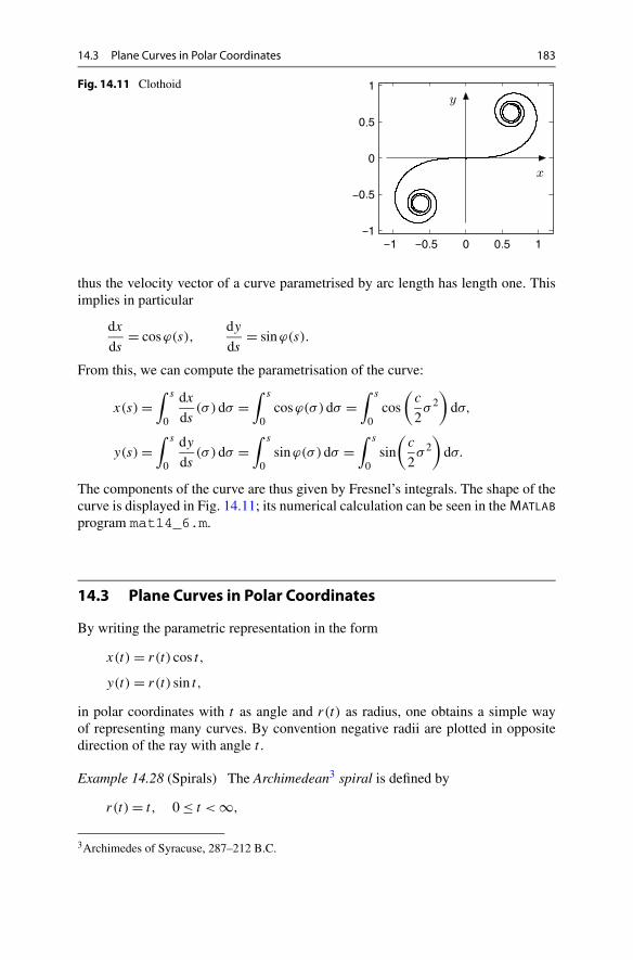
14.3 Plane Curves in Polar Coordinates 183
Fig. 14.11 Clothoid
thus the velocity vector of a curve parametrised by arc length has length one. Thisimplies in particular
dx
ds= cosϕ(s),
dy
ds= sinϕ(s).
From this, we can compute the parametrisation of the curve:
x(s) =∫ s
0
dx
ds(σ )dσ =
∫ s
0cosϕ(σ)dσ =
∫ s
0cos
(c
2σ 2
)dσ,
y(s) =∫ s
0
dy
ds(σ )dσ =
∫ s
0sinϕ(σ)dσ =
∫ s
0sin
(c
2σ 2
)dσ.
The components of the curve are thus given by Fresnel’s integrals. The shape of thecurve is displayed in Fig. 14.11; its numerical calculation can be seen in the MATLABprogram mat14_6.m.
14.3 Plane Curves in Polar Coordinates
By writing the parametric representation in the form
x(t) = r(t) cos t,
y(t) = r(t) sin t,
in polar coordinates with t as angle and r(t) as radius, one obtains a simple wayof representing many curves. By convention negative radii are plotted in oppositedirection of the ray with angle t .
Example 14.28 (Spirals) The Archimedean3 spiral is defined by
r(t) = t, 0 ≤ t < ∞,
3Archimedes of Syracuse, 287–212 B.C.

184 14 Curves
Fig. 14.12 Archimedean, logarithmic and hyperbolic spirals
the logarithmic spiral by
r(t) = et , −∞ < t < ∞,
the hyperbolic spiral by
r(t) = 1
t, 0 < t < ∞.
Typical parts of these spirals are displayed in Fig. 14.12.
Experiment 14.29 Study the behaviour of the logarithmic spiral near the originusing the zoom tool (use the M-file mat14_7.m).
Example 14.30 (Loops) Loops are obtained by choosing r(t) = cosnt , n ∈ N. InCartesian coordinates the parametric representation thus reads
x(t) = cosnt cos t,
y(t) = cosnt sin t.
The choice n = 1 results in a circle of radius 12 about ( 1
2 ,0), for odd n one obtainsn leaves, for even n one obtains 2n leaves; see Figs. 14.13 and 14.14.
The figure eight from Fig. 14.14 is obtained by r(t) = √cos 2t and r(t) =
−√cos 2t , respectively, for −π
4 < t < π4 , where the positive root gives the right
leave and the negative root the left leave. This curve is called lemniscate.
Example 14.31 (Cardioid) The cardioid is a special epicycloid, where one circle isrolling around another circle with the same radius A. Its parametric representationis
x(t) = 2A cos t + A cos 2t,
y(t) = 2A sin t + A sin 2t
for 0 ≤ t ≤ 2π . The cardioid with radius A = 1 is shown in Fig. 14.15.

14.4 Parametrised Space Curves 185
Fig. 14.13 Loops withr = cos t and r = cos 2t
Fig. 14.14 Loops withr = cos 3t and r = ±√
cos 2t
Fig. 14.15 Cardioid withA = 1
14.4 Parametrised Space Curves
In the same way as for plane curves, a parametrised curve in space is defined as acontinuous mapping of an interval [a, b] to R
3,
t �→ x(t) =⎡⎣x(t)
y(t)
z(t)
⎤⎦ , a ≤ t ≤ b.
The curve is called differentiable, if all three components t �→ x(t), t �→ y(t),t �→ z(t) are differentiable real-valued functions.
Velocity and tangent vector of a differentiable curve in space are defined as inthe planar case by
x(t) =⎡⎣x(t)
y(t)
z(t)
⎤⎦ , T(t) = x(t)
‖x(t)‖ = 1√x(t)2 + y(t)2 + z(t)2
⎡⎣x(t)
y(t)
z(t)
⎤⎦ .

186 14 Curves
Fig. 14.16 Helix with tangent, normal and binormal vector
The second derivative x(t) is the acceleration vector. In the spatial case there is anormal plane to the curve which is spanned by the normal vector
N(t) = 1
‖T(t)‖ T(t)
and the binormal vector
B(t) = T(t) × N(t),
provided that x(t) �= 0, T(t) �= 0. The formula
0 = d
dt1 = d
dt
∥∥T(t)∥∥2 = 2
⟨T(t), T(t)
⟩
(which is verified by a straightforward computation) implies that T(t) is perpendic-ular to T(t). Therefore, the three vectors (T(t),N(t),B(t)) form an orthogonal basisin R
3, called the moving frame of the curve.
Example 14.32 (Helix) The parametric representation of the helix is
x(t) =⎡⎣cos t
sin t
t
⎤⎦ , −∞ < t < ∞.
We obtain
x(t) =⎡⎣− sin t
cos t
1
⎤⎦ , T(t) = 1√
2
⎡⎣− sin t
cos t
1
⎤⎦ ,
T(t) = 1√2
⎡⎣− cos t
− sin t
0
⎤⎦ , N(t) =
⎡⎣− cos t
− sin t
0
⎤⎦

14.5 Exercises 187
with binormal vector
B(t) = 1√2
⎡⎣− sin t
cos t
1
⎤⎦ ×
⎡⎣− cos t
− sin t
0
⎤⎦ = 1√
2
⎡⎣ sin t
− cos t
1
⎤⎦ .
Figure 14.16 was drawn using the MATLAB commands
t=0:pi/100:6*pi;
plot3(cos(t),sin(t),t/10).
The Java applet Parametric curves in space offers dynamic visualising possibili-ties of those and other curves in space and of their moving frames.
14.5 Exercises
1. Find out which geometric formation is represented by the set of zeros of thepolynomial y2 −x(x2 −1) = 0. Visualise the curve in maple using the commandimplicitplot. Can you parametrise it as a continuous curve?
2. (a) Check that the following relations hold for the hyperbolic functions (Exam-ple 14.11):
(sinh t)′ = cosh t, (cosh t)′ = sinh t, cosh2 t − sinh2 t = 1.
(b) Compute the curvature κ(t) of the branch of the hyperbola
x(t) = cosh t,
y(t) = sinh t,− ∞ < t < ∞.
3. Using MATLAB or maple, investigate the shape of Lissajous figures4
x(t) = sin(w1t), y(t) = cos(w2t)
and
x(t) = sin(w1t), y(t) = cos
(w2t + π
2
).
Consider the cases w2 = w1, w2 = 2w1, w2 = 32w1 and explain the results.
The following exercises use the Java applets Parametric curves in the planeand Parametric curves in space.
4J.A. Lissajous, 1822–1880.

188 14 Curves
4. (a) Using the Java applet analyse where the cycloid
x(t) = t − 2 sin t,
y(t) = 1 − 2 cos t,− 2π ≤ t ≤ 2π
has its maximal speed (‖x(t)‖ → max), and check your result by hand.(b) Discuss and explain the shape of the loops
x(t) = cosnt cos t,
y(t) = cosnt sin t,0 ≤ t ≤ 2π
for n = 1,2,3,4,5, using the Java applets (plot the moving frame).5. Study the velocity and the acceleration of the following curves by using the Java
applet. Verify your results by computing the points where the curve has either ahorizontal tangent (x(t) �= 0, y(t) = 0) or a vertical tangent (x(t) = 0, y(t) �= 0),or is singular (x(t) = 0, y(t) = 0).(a) Cycloid:
x(t) = t − sin t,
y(t) = 1 − cos t,− 2π ≤ t ≤ 2π.
(b) Cardioid:
x(t) = 2 cos t + cos 2t,
y(t) = 2 sin t + sin 2t,0 ≤ t ≤ 2π.
6. Analyse and explain the trajectories of the curves
x(t) =[
1 − 2t2
(1 − 2t2)2
], −1 ≤ t ≤ 1,
y(t) =[
cos t
cos2 t
], 0 ≤ t ≤ 2π,
z(t) =[
t cos t
t2 cos2 t
], 6 − 2 ≤ t ≤ 2.
Are these curves (geometrically) equivalent?7. (a) Analyse the space curve
x(t) =⎡⎣ cos t
sin t
2 sin t2
⎤⎦ , 0 ≤ t ≤ 4π
using the applet.

14.5 Exercises 189
(b) Check that the curve is the intersection of the cylinder x2 + y2 = 1 with thesphere (x + 1)2 + y2 + z2 = 4.Hint. Use sin2 t
2 = 12 (1 − cos t).
8. Using MATLAB, maple or the applet, sketch and discuss the space curves
x(t) =⎡⎣t cos t
t sin t
2t
⎤⎦ , 0 ≤ t < ∞,
and
y(t) =⎡⎣cos t
sin t
0
⎤⎦ , 0 ≤ t ≤ 4π.
15Scalar-Valued Functions of Two Variables
This chapter is devoted to differential calculus of functions of two variables. Inparticular we will study geometrical objects such as tangents and tangent planes,maxima and minima, as well as linear and quadratic approximations. The restric-tion to two variables has been made for simplicity of presentation. All ideas in thisand the next chapter can easily be extended (although with slightly more notationaleffort) to the case of n variables.
We begin by studying the graph of a function with the help of vertical cuts andlevel sets. As a further tool we introduce partial derivatives, which describe the rateof change of the function in the direction of the coordinate axes. Finally, the notionof the Fréchet derivative allows us to define the tangent plane to the graph. As forfunctions of one variable, the Taylor formula plays a central role. We use it, e.g., todetermine extrema of functions of two variables.
In the entire chapter D denotes a subset of R2 and
f : D ⊂ R2 → R : (x, y) �→ z = f (x, y)
denotes a scalar-valued function of two variables. Details of vector and matrix al-gebra used in this chapter can be found in Appendices A and B.
15.1 Graph and Partial Mappings
The graph
G = {(x, y, z) ∈ D × R; z = f (x, y)
} ⊂ R3
of a function of two variables f : D → R is a surface in space, if f is sufficientlyregular. To describe the properties of this surface we consider particular curves on it.
The partial mappings
x �→ (x, b,f (x, b)
), y �→ (
a, y,f (a, y))
M. Oberguggenberger, A. Ostermann, Analysis for Computer Scientists,Undergraduate Topics in Computer Science,DOI 10.1007/978-0-85729-446-3_15, © Springer-Verlag London Limited 2011
191


15.2 Continuity 193
Example 15.1 The graph of the quadratic function
f : R2 → R : (x, y) �→ z = x2
a2− y2
b2
describes a surface in space which is shaped like a saddle and which is called ahyperbolic paraboloid. Figure 15.2 shows the graph of z = x2/4 − y2/5 with coor-dinate curves (left) as well as some level curves (right).
Experiment 15.2 With the help of the MATLAB program mat15_1.m visualise theelliptic paraboloid z = x2 + 2y2 − 4x + 1. Choose a suitable domain D and plot thegraph and some level curves.
15.2 Continuity
Like for functions in one variable (see Chap. 6), we characterise the continuity offunctions of two variables by means of sequences. Thus we need the concept ofconvergence of vector-valued sequences.
Let (an)n≥1 = (a1,a2,a3, . . .) be a sequence of points in D with terms
an = (an, bn) ∈ D ⊂ R2.
The sequence (an)n≥1 is said to converge to a = (a, b) ∈ D as n → ∞, if and onlyif both components of the sequence converge, i.e.,
limn→∞an = a and lim
n→∞bn = b.
This is denoted by
(an, bn) = an → a = (a, b) as n → ∞ or limn→∞ an = a.
Otherwise the sequence is called divergent.An example of a convergent vector-valued sequence is
limn→∞
(1
n,
2n
3n + 4
)=
(0,
2
3
).
Definition 15.3 A function f : D → R is called continuous at the point a ∈ D, if
limn→∞f (an) = f (a)
for all sequences (an)n≥1 which converge to a in D.
For continuous functions, the limit and the function sign can be interchanged.Figure 15.3 shows a function which is discontinuous along a straight line but con-tinuous everywhere else.


196 15 Scalar-Valued Functions of Two Variables
Fig. 15.5 Partiallydifferentiable, discontinuousfunction
An example is given by the function (see Fig. 15.5)
f (x, y) ={
xy
x2+y2 , (x, y) �= (0,0),
0, (x, y) = (0,0).
This function is everywhere partially differentiable. In particular, at the point(x, y) = (0,0) one obtains
∂f
∂x(0,0) = lim
x→0
f (x,0) − f (0,0)
x= 0 = lim
y→0
f (0, y) − f (0,0)
y= ∂f
∂y(0,0).
However, the function is discontinuous at (0,0). In order to see this, we choose twosequences which converge to (0,0):
an =(
1
n,
1
n
)and cn =
(1
n,−1
n
).
We have
limn→∞f (an) = lim
n→∞1/n2
2/n2= 1
2,
but also
limn→∞f (cn) = lim
n→∞−1/n2
2/n2= −1
2.
The limits do not coincide; in particular, they differ from f (0,0) = 0.
Experiment 15.7 Visualise the function given in Remark 15.6 with the help ofMATLAB and maple. Using the command
plot3d(-x*y/(x^2+y^2), x=-1..1, y=-1..1, shading=zhue)
the corresponding plot can be obtained in maple.

15.3 Partial Derivatives 197
Higher-order Partial Derivatives Let D ⊂ R2 be open and f : D → R partially
differentiable. The assignments
∂f
∂x: D → R and
∂f
∂y: D → R
themselves define scalar-valued functions of two variables. If these functions arealso partially differentiable, then f is called twice partially differentiable. The nota-tion in this case is
∂2f
∂x2= ∂
∂x
(∂f
∂x
),
∂2f
∂y∂x= ∂
∂y
(∂f
∂x
), etc.
Note that there are four partial derivatives of second order.
Definition 15.8 A function f : D → R is k-times continuously (partially) differ-entiable, denoted f ∈ Ck(D), if f is k-times partially differentiable and all partialderivatives up to order k are continuous.
Example 15.9 The function f (x, y) = exy2is arbitrarily often partially differen-
tiable, f ∈ C∞(D), and the following holds:
∂f
∂x(x, y) = exy2
y2,
∂f
∂y(x, y) = exy2
2xy,
∂2f
∂x2(x, y) = exy2
y4,
∂2f
∂y2(x, y) = exy2(
4x2y2 + 2x),
∂2f
∂y∂x(x, y) = ∂
∂y
(∂f
∂x(x, y)
)= exy2(
2xy3 + 2y),
∂2f
∂x∂y(x, y) = ∂
∂x
(∂f
∂y(x, y)
)= exy2(
2xy3 + 2y).
The identity
∂2f
∂y∂x(x, y) = ∂2f
∂x∂y(x, y)
198 15 Scalar-Valued Functions of Two Variables
which is evident in this example is generally valid for twice continuously differen-tiable functions f . This observation is also true for higher derivatives: For k-timescontinuously differentiable functions the order of differentiation of the kth partialderivatives is irrelevant (Theorem of Schwarz1); see [3, Chap. 15, Theorem 1.1].
15.4 The Fréchet Derivative
Our next topic is the study of a simultaneous variation of both variables of the func-tion. This leads to the notion of the Fréchet2 derivative. For functions of one vari-able, ϕ : R → R, the derivative was defined by the limit
ϕ′(a) = limx→a
ϕ(x) − ϕ(a)
x − a.
For functions of two variables this expression does not make sense anymore as onecannot divide by vectors. We therefore will make use of the equivalent definition ofthe derivative as a linear approximation
ϕ(x) = ϕ(a) + A · (x − a) + R(x, a)
with A = ϕ′(a) and the remainder term R(x, a) satisfying
limx→a
R(x, a)
|x − a| = 0.
This formula can be generalised to functions of two variables.
Definition 15.10 Let D ⊂ R2 be open and f : D → R. The function f is called
Fréchet differentiable at the point (a, b) ∈ D, if there exists a linear mappingA : R
2 → R such that
f (x, y) = f (a, b) + A(x − a, y − b) + R(x, y;a, b)
with a remainder R(x, y;a, b) fulfilling the condition
lim(x,y)→(a,b)
R(x, y;a, b)√(x − a)2 + (y − b)2
= 0.
The linear mapping A is called derivative of f at the point (a, b). Instead of A
we also write Df (a, b). The (1 × 2)-matrix of the linear mapping is called theJacobian3 of f . We denote it by f ′(a, b).
1H.A. Schwarz, 1843–1921.2M. Fréchet, 1878–1973.3C.G.J. Jacobi, 1804–1851.
15.4 The Fréchet Derivative 199
The questions whether the derivative of a function is unique, and how it can becalculated, are answered in the following proposition.
Proposition 15.11 Let D ⊂ R2 be open and f : D → R. If f is Fréchet differen-
tiable at (x, y) ∈ D, then f is also partially differentiable at (x, y) and
f ′(x, y) =[∂f
∂x(x, y),
∂f
∂y(x, y)
].
The components of the Jacobian are the partial derivatives. In particular, the Jaco-bian and consequently the Fréchet derivative are unique.
Proof Exemplarily, we compute the second component and show that
(f ′(x, y)
)2 = ∂f
∂y(x, y).
Since f is Fréchet differentiable at (x, y), it holds that
f (x, y + h) = f (x, y) + f ′(x, y)
[0h
]+ R(x, y + h;x, y).
Therefore
f (x, y + h) − f (x, y)
h− (
f ′(x, y))
2 = R(x, y + h;x, y)
h→ 0 as h → 0.
Consequently f is partially differentiable with respect to y, and the second compo-nent of the Jacobian is the partial derivative of f with respect to y. �
The next proposition follows immediately from the identity
lim(x,y)→(a,b)
f (x, y)
= lim(x,y)→(a,b)
(f (a, b) + Df (a, b)(x − a, y − b) + R(x, y;a, b)
)
= f (a, b).
Proposition 15.12 If f is Fréchet differentiable, then f is continuous.
In particular, the function
f (x, y) ={
xy
x2+y2 , (x, y) �= (0,0),
0, (x, y) = (0,0)
is not Fréchet differentiable at the point (0,0).Fréchet differentiability follows from partial differentiability under certain regu-
larity assumptions. In fact, one can show that a continuously partially differentiablefunction is Fréchet differentiable; see [4, Chap. 7, Theorem 7.12].

200 15 Scalar-Valued Functions of Two Variables
Example 15.13 The function f : R2 → R : (x, y) �→ x2e3y is Fréchet differentiable;
its derivative is
f ′(x, y) = [2xe3y,3x2e3y
] = xe3y[2,3x].
Example 15.14 The affine function f : R2 → R with
f (x, y) = αx + βy + γ = [α,β][x
y
]+ γ
is Fréchet differentiable, and f ′(x, y) = [α,β].
Example 15.15 The quadratic function f : R2 → R with
f (x, y) = αx2 + 2βxy + γy2 + δx + εy + ζ
= [x, y][
α β
β γ
][x
y
]+ [δ, ε]
[x
y
]+ ζ
is Fréchet differentiable with the Jacobian
f ′(x, y) = [2αx + 2βy + δ,2βx + 2γy + ε] = 2[x, y][
α β
β γ
]+ [δ, ε].
The Chain Rule Now we are in the position to generalise the chain rule to thecase of two variables.
Proposition 15.16 Let D ⊂ R2 be open and f : D → R : (x, y) �→ f (x, y) Fréchet
differentiable. Furthermore, let I ⊂ R be an open interval and ϕ,ψ : I → R differ-entiable. Then the composition of functions
F : I → R : t �→ F(t) = f(ϕ(t),ψ(t)
)
is also differentiable and
dF
dt(t) = ∂f
∂x
(ϕ(t),ψ(t)
)dϕ
dt(t) + ∂f
∂y
(ϕ(t),ψ(t)
)dψ
dt(t).
Proof From Fréchet differentiability of f it follows that
F(t + h) − F(t) = f(ϕ(t + h),ψ(t + h)
) − f(ϕ(t),ψ(t)
)
= f ′(ϕ(t),ψ(t))[
ϕ(t + h) − ϕ(t)
ψ(t + h) − ψ(t)
]
+ R(ϕ(t + h),ψ(t + h);ϕ(t),ψ(t)
).

15.4 The Fréchet Derivative 201
We divide this expression by h and subsequently examine the limit as h → 0. Letg(t, h) = (ϕ(t +h)−ϕ(t))2 + (ψ(t +h)−ψ(t))2. Then, due to the differentiabilityof f , ϕ and ψ , we have
limh→0
R(ϕ(t + h),ψ(t + h);ϕ(t),ψ(t))√g(t, h)
·√
g(t, h)
h= 0.
Therefore, the function F is differentiable and the formula stated in the propositionis valid. �
Example 15.17 Let D ⊂ R2 be an open set that contains the circle x2 + y2 = 1 and
let f : D → R be a differentiable function. Then the restriction F of f to the circle
F : R → R : t �→ f (cos t, sin t)
is differentiable as a function of the angle t and
dF
dt(t) = −∂f
∂x(cos t, sin t) · sin t + ∂f
∂y(cos t, sin t) · cos t.
For instance, for f (x, y) = x2 − y2 the derivative is dFdt
(t) = −4 cos t sin t .
Interpretation of the Fréchet Derivative Using the Fréchet derivative, we ob-tain, like in the case of one variable, the linear approximation g(x, y) to the graphof the function at (a, b):
g(x, y) = f (a, b) + f ′(a, b)
[x − a
y − b
]≈ f (x, y).
Now we want to interpret the plane
z = f (a, b) + f ′(a, b)
[x − a
y − b
]
geometrically. In order to do this we use the fact that the components of the Jacobianare the partial derivatives. Because of this, we can write the above equation as
z = f (a, b) + ∂f
∂x(a, b) · (x − a) + ∂f
∂y(a, b) · (y − b),
or, alternatively, in parametric form (x − a = λ, y − b = μ):
⎡⎣x
y
z
⎤⎦ =
⎡⎣ a
b
f (a, b)
⎤⎦ + λ
⎡⎣ 1
0∂f∂x
(a, b)
⎤⎦ + μ
⎡⎣ 0
1∂f∂y
(a, b)
⎤⎦ .
202 15 Scalar-Valued Functions of Two Variables
The plane intersects the graph of f at the point (a, b, f (a, b)) and is spanned by thetangent vectors to the coordinate curves. The equation
z = f (a, b) + ∂f
∂x(a, b) · (x − a) + ∂f
∂y(a, b) · (y − b)
consequently describes the tangent plane to the graph of f at the point (a, b).The example shows that the graph of a function which is Fréchet differentiable
at the point (x, y) possesses a tangent plane at this point. Note that the existence oftangents to the coordinate curves does not imply the existence of a tangent plane;see Remark 15.6.
Example 15.18 We calculate the tangent plane at a point on the northern hemisphere(with radius r)
f (x, y) = z =√
r2 − x2 − y2.
Let c = f (a, b) = √r2 − a2 − b2. The partial derivatives of f at (a, b) are
∂f
∂x(a, b) = − a√
r2 − a2 − b2= −a
c,
∂f
∂y(a, b) = − b√
r2 − a2 − b2= −b
c.
Therefore, the equation of the tangent plane is
z = c − a
c(x − a) − b
c(y − b),
or alternatively
a(x − a) + b(y − b) + c(z − c) = 0.
The last formula actually holds for all points on the surface of the sphere.
15.5 Directional Derivative and Gradient
So far functions f : D ⊂ R2 → R were defined on R
2 as a point space. For thepurpose of directional derivatives it is useful and customary to write the arguments(x, y) ∈ R
2 as position vectors x = [x, y]T. In this way each function f : D ⊂ R2 →
R can also be considered as a function of column vectors. We identify these twofunctions and will not distinguish between f (x, y) and f (x) henceforth.
In Sect. 15.3 we have defined partial derivatives along coordinate axes. Now wewant to generalise this concept to differentiation in any direction.

15.5 Directional Derivative and Gradient 203
Definition 15.19 Let D ⊂ R2 be open, x = [x, y]T ∈ D and f : D → R. Further-
more, let v ∈ R2 with ‖v‖ = 1. The limit
∂vf (x) = ∂f
∂v(x) = lim
h→0
f (x + hv) − f (x)
h
= limh→0
f (x + hv1, y + hv2) − f (x, y)
h
(in case it exists) is called the directional derivative of f at x in the direction v.
The partial derivatives are special cases of the directional derivative, namely thederivatives in direction of the coordinate axes.
The directional derivative ∂vf (x) describes the rate of change of the function f
at the point x in the direction of v. Indeed, this can been seen from the following.Consider the straight line {x + tv|t ∈ R} ⊂ R
2 and the function
g(t) = f (x + tv) (f restricted to this straight line)
with g(0) = f (x). Then
g′(0) = limh→0
g(h) − g(0)
h= lim
h→0
f (x + hv) − f (x)
h= ∂vf (x).
Next we clarify how the directional derivative can be computed. In order to do thiswe need the following definition.
Definition 15.20 Let D ⊂ R2 be open and f : D → R partially differentiable. The
vector
∇f (x, y) =⎡⎣
∂f∂x
(x, y)
∂f∂y
(x, y)
⎤⎦ = f ′(x, y)T
is called the gradient of f .
Proposition 15.21 Let D ⊂ R2 be open, v = [v1, v2]T ∈ R
2, ‖v‖ = 1 and letf : D → R be Fréchet differentiable at x = [x, y]T. Then
∂vf (x) = ⟨∇f (x),v⟩ = f ′(x, y)v = ∂f
∂x(x, y)v1 + ∂f
∂y(x, y)v2.
Proof Since f is Fréchet differentiable at x, the following holds:
f (x + hv) = f (x) + f ′(x) · hv + R(x + hv1, y + hv2;x, y)
and hence
f (x + hv) − f (x)
h= f ′(x) · v + R(x + hv1, y + hv2;x, y)
h.
Letting h → 0 proves the desired assertion. �

204 15 Scalar-Valued Functions of Two Variables
Fig. 15.6 Geometricinterpretation of ∇f
Proposition 15.22 (Geometric interpretation of ∇) Let D ⊂ R2 be open and let
f : D → R be continuously differentiable at x = (x, y) with f ′(x) �= [0,0]. Then∇f (x) is perpendicular to the level curve Nf (x) = {x ∈ R
2; f (x) = f (x)} andpoints in the direction of the steepest ascent of f ; see Fig. 15.6.
Proof Let v be a tangent vector to the level curve at the point x. From the implicitfunction theorem (see [4, Chap. 14.1]) it follows that Nf (x) can be parametrised asa differentiable curve γ (t) = [x(t), y(t)]T, with
γ (0) = x and γ (0) = v,
in a neighbourhood of x. Thus, for all t near t = 0,
f(γ (t)
) = f (x) = const.
Since f and γ are differentiable, it follows from the chain rule (Proposition 15.16)that
0 = d
dtf
(γ (t)
)∣∣t=0 = f ′(γ (0)
)γ (0) = ⟨∇f (x),v
⟩,
because γ (0) = x and γ (0) = v. Hence ∇f (x) is perpendicular to v. Let w ∈ R2 be
a further unit vector. Then
∂wf (x) = ∂f
∂w(x) = ⟨∇f (x),w
⟩ = ∥∥∇f (x)∥∥ · ‖w‖ · cos�,
where � denotes the angle enclosed by ∇f (x) and w. From this formula one de-duces that ∂wf (x) is maximal if and only if cos� = 1, which means that ∇f (x) =λw for some λ > 0. �
Example 15.23 Let f (x, y) = x2 + y2. Then ∇f (x, y) = 2[x, y]T.
15.6 The Taylor Formula in Two Variables
Let f : D ⊂ R2 → R be a function of two variables. In the following calculation we
assume that f is at least three times continuously differentiable. In order to expand

15.6 The Taylor Formula in Two Variables 205
f (x + h,y + k) into a Taylor series in a neighbourhood of (x, y), we first fix thesecond variable and expand with respect to the first:
f (x +h,y +k) = f (x, y +k)+ ∂f
∂x(x, y +k) ·h+ 1
2
∂2f
∂x2(x, y +k) ·h2 + O
(h3).
Then we also expand the terms on the right-hand side with respect to the secondvariable (while fixing the first one):
f (x, y + k) = f (x, y) + ∂f
∂y(x, y) · k + 1
2
∂2f
∂y2(x, y) · k2 + O
(k3),
∂f
∂x(x, y + k) = ∂f
∂x(x, y) + ∂2f
∂y∂x(x, y) · k + O
(k2),
∂2f
∂x2(x, y + k) = ∂2f
∂x2(x, y) + O(k).
Inserting these expressions into the equation above, we obtain
f (x + h,y + k) = f (x, y) + ∂f
∂x(x, y) · h + ∂f
∂y(x, y) · k
+ 1
2
∂2f
∂x2(x, y) · h2 + 1
2
∂2f
∂y2(x, y) · k2 + ∂2f
∂y∂x(x, y) · hk
+ O(h3) + O
(h2k
) + O(hk2) + O
(k3).
In matrix-vector notation we can also write this equation as
f (x + h,y + k) = f (x, y) + f ′(x, y)
[h
k
]+ 1
2[h, k] · Hf (x, y)
[h
k
]+ · · ·
with the Hessian matrix4
Hf (x, y) =⎡⎢⎣
∂2f
∂x2 (x, y)∂2f∂y∂x
(x, y)
∂2f∂x∂y
(x, y)∂2f
∂y2 (x, y)
⎤⎥⎦
collecting the second-order partial derivatives. By the above assumptions, thesederivatives are continuous. Thus the Hessian matrix is symmetric due to Schwarz’stheorem.
Example 15.24 We compute the second-order approximation to the functionf : R
2 → R : (x, y) �→ x2 siny at the point (a, b) = (2,0). The partial derivativesare given in Table 15.1.
4L.O. Hesse, 1811–1874.

206 15 Scalar-Valued Functions of Two Variables
Table 15.1 Partial derivatives of z = x2 siny
f∂f∂x
∂f∂y
∂2f
∂x2∂2f∂y∂x
∂2f
∂y2
General x2 siny 2x siny x2 cosy 2 siny 2x cosy −x2 siny
At (2,0) 0 0 4 0 4 0
Therefore, the quadratic approximation g(x, y) ≈ f (x, y) is given by the formula
g(x, y) = f (2,0) + f ′(2,0)
[x − 2
y
]+ 1
2[x − 2, y] · Hf (2,0)
[x − 2
y
]
= 0 + [0,4][x − 2
y
]+ 1
2[x − 2, y]
[0 44 0
][x − 2
y
]
= 4y + 4y(x − 2) = 4y(x − 1).
15.7 Local Maxima and Minima
Let D ⊂ R2 be open and f : D → R. In this section we investigate the graph of the
function f with respect to maxima and minima.
Definition 15.25 The scalar function f has a local maximum (respectively, localminimum) at (a, b) ∈ D, if
f (x, y) ≤ f (a, b) (respectively, f (x, y) ≥ f (a, b))
for all (x, y) in a neighbourhood of (a, b). The maximum (minimum) is called iso-lated, if (a, b) is the only point in a neighbourhood with this property.
Figure 15.7 shows a few typical examples. One observes that the existence ofa horizontal tangent plane is a necessary condition for extrema (i.e., maxima orminima) of differentiable functions.
Proposition 15.26 Let f be partially differentiable. If f has a local maximum orminimum at (a, b) ∈ D, then the partial derivatives vanish at (a, b):
∂f
∂x(a, b) = ∂f
∂y(a, b) = 0.
If, in addition, f is Fréchet differentiable, then f ′(a, b) = [0,0], i.e., f has a hori-zontal tangent plane at (a, b).
Proof Due to the assumptions, the function g(h) = f (a + h,b) has an extremum ath = 0. Thus, Proposition 8.2 implies
g′(0) = ∂f
∂x(a, b) = 0.
Likewise one can show that ∂f∂y
(a, b) = 0. �


208 15 Scalar-Valued Functions of Two Variables
If w �= 0, we substitute v = tw with t ∈ R and obtain
αt2w2 + 2βtw2 + γw2 > 0,
or, alternatively (multiplying by α > 0 and simplifying by w2),
t2α2 + 2tαβ + αγ > 0.
Therefore,
(tα + β)2 + αγ − β2 > 0
for all t ∈ R. The left-hand side is smallest for t = −β/α. Inserting this we obtainthe second condition
detHf (a) = αγ − β2 > 0
in terms of the determinant; see Sect. 23.1.We have thus shown the following result.
Proposition 15.28 The function f has an isolated local minimum at the stationarypoint a, if the conditions
∂2f
∂x2(a) > 0 and detHf (a) > 0
are fulfilled.
By replacing f by −f one gets the corresponding result for isolated maxima.
Proposition 15.29 The function f has an isolated local maximum at the stationarypoint a, if the conditions
∂2f
∂x2(a) < 0 and detHf (a) > 0
are fulfilled.
In a similar way one can prove the following assertion.
Proposition 15.30 The stationary point a of the function f is a saddle point, ifdetHf (a) < 0.
If the determinant of the Hessian matrix equals zero, the behaviour of the functionneeds to be investigated along vertical cuts. One example is given in Exercise 9.

15.8 Exercises 209
Example 15.31 We determine the maxima, minima and saddle points of the functionf (x, y) = x6 + y6 − 3x2 − 3y2. The condition
f ′(x, y) = [6x5 − 6x,6y5 − 6y
] = [0,0]gives the following nine stationary points:
x1 = 0, x2,3 = ±1, y1 = 0, y2,3 = ±1.
The Hessian matrix of the function is
Hf (x, y) =[
30x4 − 6 00 30y4 − 6
].
Applying the criteria of Propositions 15.28 through 15.30, we obtain the followingresults. The point (0,0) is an isolated local maximum of f , the points (−1,−1),(−1,1), (1,−1) and (1,1) are isolated local minima, and the points (−1,0), (1,0),(0,−1) and (0,1) are saddle points. The reader is advised to visualise this functionwith maple.
15.8 Exercises
1. Compute the partial derivatives of the functions
f (x, y) = arcsin
(y
x
), g(x, y) = log
1√x2 + y2
.
Verify your results with maple.2. Show that the function
v(x, t) = 1√t
exp
(−x2
4t
)
satisfies the heat equation
∂v
∂t= ∂2v
∂x2
for t > 0 and x ∈ R.3. Show that the function w(x, t) = g(x − kt) satisfies the transport equation
∂w
∂t+ k
∂w
∂x= 0
for any differentiable function g.
210 15 Scalar-Valued Functions of Two Variables
4. Show that the function g(x, y) = log(x2 + 2y2) satisfies the equation
∂2g
∂x2+ 1
2
∂2g
∂y2= 0
for (x, y) �= (0,0).5. Represent the ellipsoid x2 + 2y2 + z2 = 1 as graph of a function (x, y) �→
f (x, y). Distinguish between positive and negative z-coordinates, respectively.Compute the partial derivatives of f , and sketch the level curves of f . Find thedirection in which ∇f points.
6. Solve Exercise 5 for the hyperboloid x2 + 2y2 − z2 = 1.7. Consider the function f (x, y) = ye2x−y , where x = x(t) and y = y(t) are dif-
ferentiable functions satisfying
x(0) = 2, y(0) = 4, x(0) = −1, y(0) = 4.
From this information compute the derivative of z(t) = f (x(t), y(t)) at thepoint t = 0.
8. Find all stationary points of the function
f (x, y) = x3 − 3xy2 + 6y.
Determine whether they are maxima, minima or saddle points.9. Investigate the function
f (x, y) = x4 − 3x2y + y3
for local extrema and saddle points. Visualise the graph of the function.Hint. To study the behaviour of the function at (0,0) consider the partial map-pings f (x,0) and f (0, y).
10. Determine for the function
f (x, y) = x2ey/3(y − 3) − 1
2y2
(a) the gradient and the Hessian matrix(b) the second-order Taylor approximation at (0,0)
(c) all stationary points. Find out whether they are maxima, minima or saddlepoints.
16Vector-Valued Functions of Two Variables
In this section we briefly touch upon the theory of vector-valued functions in severalvariables. To simplify matters we limit ourselves again to the case of two variables.
First, we define vector fields in the plane and extend the notions of continuityand differentiability to vector-valued functions. Then we discuss Newton’s methodin two variables. As an application we compute a common zero of two nonlinearfunctions. Finally, as an extension of Sect. 15.1, we show how smooth surfaces canbe described mathematically with the help of parametrisations.
For the required basic notions of vector and matrix algebra we refer to Appen-dices A and B.
16.1 Vector Fields and the Jacobian
In the entire section D denotes an open subset of R2 and
F : D ⊂ R2 → R
2 : (x, y) �→[u
v
]= F(x, y) =
[f (x, y)
g(x, y)
]
a vector-valued function of two variables with values in R2. Such functions are also
called vector fields since they assign a vector to every point in the plane. Importantapplications are provided in physics. For example, the velocity field of a flowingliquid or the gravitational field are mathematically described as vector fields.
In the previous chapter we have already encountered a vector field, namely thegradient of a scalar-valued function of two variables f : D → R : (x, y) �→ f (x, y).For a partially differentiable function f the gradient
F = ∇f : D → R2 : (x, y) �→
⎡⎣
∂f∂x
(x, y)
∂f∂y
(x, y)
⎤⎦
is obviously a vector field.Continuity and differentiability of vector fields are defined componentwise.
M. Oberguggenberger, A. Ostermann, Analysis for Computer Scientists,Undergraduate Topics in Computer Science,DOI 10.1007/978-0-85729-446-3_16, © Springer-Verlag London Limited 2011
211

212 16 Vector-Valued Functions of Two Variables
Definition 16.1 The function
F : D ⊂ R2 → R
2 : (x, y) �→ F(x, y) =[f (x, y)
g(x, y)
]
is called continuous (or partially differentiable or Fréchet differentiable, respec-tively) if and only if its two components f : D → R and g : D → R have the cor-responding property, i.e., they are continuous (or partially differentiable or Fréchetdifferentiable, respectively).
If both f and g are Fréchet differentiable, one has the linearisations
f (x, y) = f (a, b) + [ ∂f∂x
(a, b),∂f∂y
(a, b)][
x − a
y − b
]+ R1(x, y;a, b),
g(x, y) = g(a, b) + [ ∂g∂x
(a, b),∂g∂y
(a, b)][
x − a
y − b
]+ R2(x, y;a, b)
for (x, y) close to (a, b) with remainder terms R1 and R2. If one combines thesetwo formulae to one formula using matrix-vector notation, one obtains
[f (x, y)
g(x, y)
]=
[f (a, b)
g(a, b)
]+
⎡⎣
∂f∂x
(a, b)∂f∂y
(a, b)
∂g∂x
(a, b)∂g∂y
(a, b)
⎤⎦
[x − a
y − b
]+
[R1(x, y;a, b)
R2(x, y;a, b)
],
or in short-hand notation
F(x, y) = F(a, b) + F′(a, b)
[x − a
y − b
]+ R(x, y;a, b)
with the remainder term R(x, y;a, b) and the (2×2)-Jacobian
F′(a, b) =⎡⎣
∂f∂x
(a, b)∂f∂y
(a, b)
∂g∂x
(a, b)∂g∂y
(a, b)
⎤⎦ .
The linear mapping defined by this matrix is called (Fréchet) derivative of the func-tion F at the point (a, b). The remainder term R has the property
lim(x,y)→(a,b)
√R1(x, y;a, b)2 + R2(x, y;a, b)2√
(x − a)2 + (y − b)2= 0.
Example 16.2 (Polar coordinates) The mapping
F : R2 → R
2 : (r,φ) �→[x
y
]=
[r cosϕ
r sinϕ
]

16.2 Newton’s Method in Two Variables 213
is (everywhere) differentiable with derivative (Jacobian)
F′(r, ϕ) =[
cosϕ −r sinϕ
sinϕ r cosϕ
].
16.2 Newton’s Method in Two Variables
The linearisation
F(x, y) ≈ F(a, b) + F′(a, b)
[x − a
y − b
]
is the key for solving nonlinear equations in two (or more) unknowns. In this section,we derive Newton’s method for determining the zeros of a function
F(x, y) =[f (x, y)
g(x, y)
]
of two variables and two components.
Example 16.3 (Intersection of a circle with a hyperbola) Consider the circle x2 +y2 = 4 and the hyperbola xy = 1. The points of intersection are the zeros of thevector equation F(x, y) = 0 with
F : R2 → R
2 : F(x, y) =[f (x, y)
g(x, y)
]=
[x2 + y2 − 4
xy − 1
].
The level curves f (x, y) = 0 and g(x, y) = 0 are sketched in Fig. 16.1.
Newton’s method for determining the zeros is based on the following idea. Fora starting value (x0, y0) which is sufficiently close to the solution, one computes animproved value by replacing the function by its linear approximation at (x0, y0)
F(x, y) ≈ F(x0, y0) + F′(x0, y0)
[x − x0y − y0
].
The zero of the linearisation
F(x0, y0) + F′(x0, y0)
[x − x0y − y0
]=
[00
]
is taken as improved approximation (x1, y1), so
F′(x0, y0)
[x1 − x0y1 − y0
]= −F(x0, y0),
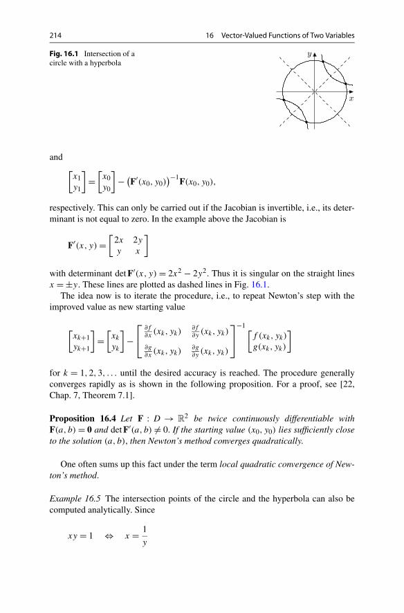
214 16 Vector-Valued Functions of Two Variables
Fig. 16.1 Intersection of acircle with a hyperbola
and[x1y1
]=
[x0y0
]− (
F′(x0, y0))−1F(x0, y0),
respectively. This can only be carried out if the Jacobian is invertible, i.e., its deter-minant is not equal to zero. In the example above the Jacobian is
F′(x, y) =[
2x 2y
y x
]
with determinant det F′(x, y) = 2x2 − 2y2. Thus it is singular on the straight linesx = ±y. These lines are plotted as dashed lines in Fig. 16.1.
The idea now is to iterate the procedure, i.e., to repeat Newton’s step with theimproved value as new starting value
[xk+1yk+1
]=
[xk
yk
]−
⎡⎣
∂f∂x
(xk, yk)∂f∂y
(xk, yk)
∂g∂x
(xk, yk)∂g∂y
(xk, yk)
⎤⎦
−1 [f (xk, yk)
g(xk, yk)
]
for k = 1,2,3, . . . until the desired accuracy is reached. The procedure generallyconverges rapidly as is shown in the following proposition. For a proof, see [22,Chap. 7, Theorem 7.1].
Proposition 16.4 Let F : D → R2 be twice continuously differentiable with
F(a, b) = 0 and det F′(a, b) �= 0. If the starting value (x0, y0) lies sufficiently closeto the solution (a, b), then Newton’s method converges quadratically.
One often sums up this fact under the term local quadratic convergence of New-ton’s method.
Example 16.5 The intersection points of the circle and the hyperbola can also becomputed analytically. Since
xy = 1 ⇔ x = 1
y
16.3 Parametric Surfaces 215
we may insert x = 1/y into the equation x2 + y2 = 4 to obtain the biquadraticequation
y4 − 4y2 + 1 = 0.
By substituting y2 = u the equation is easily solvable. The intersection point withthe largest x-component has the coordinates
x =√
2 + √3 = 1.93185165257813657 . . . ,
y =√
2 − √3 = 0.51763809020504152 . . . .
Application of Newton’s method with starting values x0 = 2 and y0 = 1 yieldsthe above solution in five steps with 16 digits accuracy. The quadratic convergencecan be observed from the fact that the number of correct digits doubles with eachstep.
x y Error
2.000000000000000 1.000000000000000 4.871521418175E-001
2.000000000000000 5.000000000000000E-001 7.039388810410E-002
1.933333333333333 5.166666666666667E-001 1.771734052060E-003
1.931852741096439 5.176370548219287E-001 1.502295005704E-006
1.931851652578934 5.176380902042443E-001 1.127875985998E-012
1.931851652578136 5.176380902050416E-001 2.220446049250E-016
Experiment 16.6 Using the MATLAB programs mat16_1.m and mat16_2.mcompute the intersection points from Example 16.3. Experiment with different start-ing values and this way try to determine all four solutions to the problem. Whathappens if the starting value is chosen to be (x0, y0) = (1,1)?
16.3 Parametric Surfaces
In Sect. 15.1 we investigated surfaces as graphs of functions f : D ⊂ R2 → R.
However, similar to the case of curves, this concept is too narrow to represent morecomplicated surfaces. The remedy is to use parametrisations like it was done forcurves.
The starting point for the construction of a parametric surface is a (component-wise) continuous mapping
(u, v) �→ x(u, v) =⎡⎣x(u, v)
y(u, v)
z(u, v)
⎤⎦

216 16 Vector-Valued Functions of Two Variables
of a parameter domain D ⊂ R2 to R
3. By fixing one parameter, u = u0 or v = v0,at a time, one obtains coordinate curves in space
u �→ x(u, v0) u-curve,
v �→ x(u0, v) v-curve.
Definition 16.7 A regular parametric surface is defined by a mappingD ⊂ R
2 → R3 : (u, v) �→ x(u, v) which satisfies the following conditions:
(a) The mapping (u, v) �→ x(u, v) is injective.(b) The u-curves and the v-curves are continuously differentiable.(c) The tangent vectors to the u-curves and v-curves are linearly independent at
every point (thus, they always span a plane).
These conditions guarantee that the parametric surface is indeed a two-dimen-sional smooth subset of R
3.
Example 16.8 (Surfaces of rotation) By rotation of the graph of a continuously dif-ferentiable, positive function z �→ h(z), a < z < b, around the z-axis, one obtains asurface of rotation with parametrisation
D = (a, b) × (0,2π), x(u, v) =⎡⎣h(u) cosv
h(u) sinv
u
⎤⎦ .
The v-curves are horizontal circles, the u-curves are the generator lines. Note thatthe generator line corresponding to the angle v = 0 has been removed to ensurecondition (a). To verify condition (c) we compute the cross product of the tangentvectors to the u- and the v-curves
∂x∂u
× ∂x∂v
=⎡⎣h′(u) cosv
h′(u) sinv
1
⎤⎦ ×
⎡⎣−h(u) sinv
h(u) cosv
0
⎤⎦ =
⎡⎣−h(u) cosv
−h(u) sinv
h(u)h′(u)
⎤⎦ �= 0.
Due to h(u) > 0 this vector is not zero; the two tangent vectors are hence notcollinear.
Figure 16.2 shows the surface of rotation which is generated by h(u) = 0.4 +cos(4πu)/3, u ∈ (0,1). In MATLAB one advantageously uses the command cylin-der in combination with the command mesh for the representation of such sur-faces.
Example 16.9 (The sphere) The sphere of radius R is obtained by the parametrisa-tion
D = (0,π) × (0,2π), x(u, v) =⎡⎣R sinu cosv
R sinu sinv
R cosu
⎤⎦ .


218 16 Vector-Valued Functions of Two Variables
2. Program Newton’s method in several variables and test the program on the prob-lem
x2 + siny = 4,
xy = 1
with starting values x = 2 and y = 1. If you are working in MATLAB, you cansolve this question by modifying mat16_2.m.
17Integration of Functions of Two Variables
In Sect. 11.3 we have shown how to calculate the volume of solids of revolution. Ifthere is no rotational symmetry, however, one needs an extension of integral calcu-lus to functions of two variables. This arises, for example, if one wants to find thevolume of a solid that lies between a domain D in the (x, y)-plane and the graphof a non-negative function z = f (x, y). In this section we will extend the notion ofRiemann integrals from Chap. 11 to double integrals of functions of two variables.Important tools for the computation of double integrals are their representation asiterated integrals and the transformation formula (change of coordinates). The inte-gration of functions of several variables occurs in numerous applications, a few ofwhich we will discuss.
17.1 Double Integrals
We start with the integration of a real-valued function z = f (x, y) which is definedon a rectangle R = [a, b]×[c, d]. More general domains of integration D ⊂ R
2 willbe discussed below. Since we know from Sect. 11.1 that Riemann integrable func-tions are necessarily bounded, we assume in this whole section that f is bounded.If f is non-negative, the integral should be interpretable as the volume of the solidwith base R and top surface given by the graph of f (see Fig. 17.2). This motivatesthe following approach in which the solid is approximated by a sum of cuboids.
We place a rectangular grid G over the domain R by partitioning the intervals[a, b] and [c, d] like in Sect. 11.1:
Zx : a = x0 < x1 < x2 < · · · < xn−1 < xn = b,
Zy : c = y0 < y1 < y2 < · · · < ym−1 < ym = d.
The rectangular grid is made up of the small rectangles
[xi−1, xi] × [yj−1, yj ], i = 1, . . . , n, j = 1, . . . ,m.
M. Oberguggenberger, A. Ostermann, Analysis for Computer Scientists,Undergraduate Topics in Computer Science,DOI 10.1007/978-0-85729-446-3_17, © Springer-Verlag London Limited 2011
219

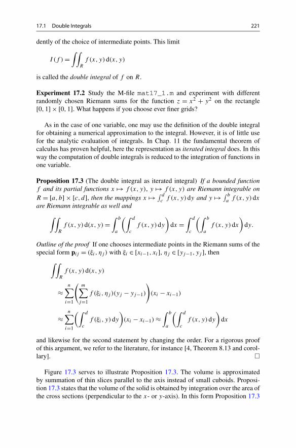
17.1 Double Integrals 221
dently of the choice of intermediate points. This limit
I (f ) =∫ ∫
R
f (x, y)d(x, y)
is called the double integral of f on R.
Experiment 17.2 Study the M-file mat17_1.m and experiment with differentrandomly chosen Riemann sums for the function z = x2 + y2 on the rectangle[0,1] × [0,1]. What happens if you choose ever finer grids?
As in the case of one variable, one may use the definition of the double integralfor obtaining a numerical approximation to the integral. However, it is of little usefor the analytic evaluation of integrals. In Chap. 11 the fundamental theorem ofcalculus has proven helpful, here the representation as iterated integral does. In thisway the computation of double integrals is reduced to the integration of functions inone variable.
Proposition 17.3 (The double integral as iterated integral) If a bounded functionf and its partial functions x �→ f (x, y), y �→ f (x, y) are Riemann integrable onR = [a, b] × [c, d], then the mappings x �→ ∫ d
cf (x, y)dy and y �→ ∫ b
af (x, y)dx
are Riemann integrable as well and
∫ ∫R
f (x, y)d(x, y) =∫ b
a
(∫ d
c
f (x, y)dy
)dx =
∫ d
c
(∫ b
a
f (x, y)dx
)dy.
Outline of the proof If one chooses intermediate points in the Riemann sums of thespecial form pij = (ξi, ηj ) with ξi ∈ [xi−1, xi], ηj ∈ [yj−1, yj ], then
∫ ∫R
f (x, y)d(x, y)
≈n∑
i=1
(m∑
j=1
f (ξi, ηj )(yj − yj−1)
)(xi − xi−1)
≈n∑
i=1
(∫ d
c
f (ξi, y)dy
)(xi − xi−1) ≈
∫ b
a
(∫ d
c
f (x, y)dy
)dx
and likewise for the second statement by changing the order. For a rigorous proofof this argument, we refer to the literature, for instance [4, Theorem 8.13 and corol-lary]. �
Figure 17.3 serves to illustrate Proposition 17.3. The volume is approximatedby summation of thin slices parallel to the axis instead of small cuboids. Proposi-tion 17.3 states that the volume of the solid is obtained by integration over the area ofthe cross sections (perpendicular to the x- or y-axis). In this form Proposition 17.3


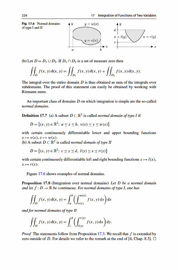
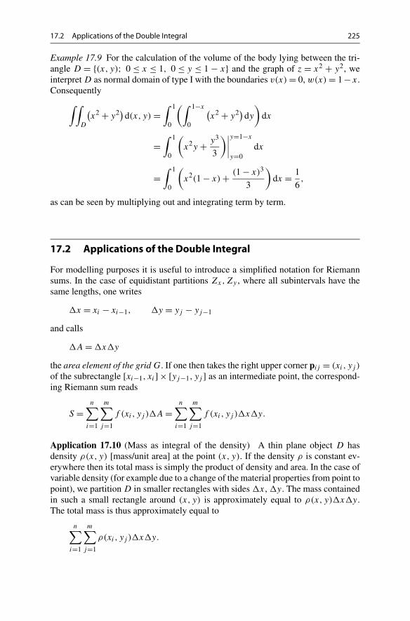
17.2 Applications of the Double Integral 225
Example 17.9 For the calculation of the volume of the body lying between the tri-angle D = {(x, y); 0 ≤ x ≤ 1, 0 ≤ y ≤ 1 − x} and the graph of z = x2 + y2, weinterpret D as normal domain of type I with the boundaries v(x) = 0, w(x) = 1−x.Consequently
∫ ∫D
(x2 + y2)d(x, y) =
∫ 1
0
(∫ 1−x
0
(x2 + y2)dy
)dx
=∫ 1
0
(x2y + y3
3
)∣∣∣∣y=1−x
y=0dx
=∫ 1
0
(x2(1 − x) + (1 − x)3
3
)dx = 1
6,
as can be seen by multiplying out and integrating term by term.
17.2 Applications of the Double Integral
For modelling purposes it is useful to introduce a simplified notation for Riemannsums. In the case of equidistant partitions Zx,Zy , where all subintervals have thesame lengths, one writes
�x = xi − xi−1, �y = yj − yj−1
and calls
�A = �x�y
the area element of the grid G. If one then takes the right upper corner pij = (xi, yj )
of the subrectangle [xi−1, xi] × [yj−1, yj ] as an intermediate point, the correspond-ing Riemann sum reads
S =n∑
i=1
m∑j=1
f (xi, yj )�A =n∑
i=1
m∑j=1
f (xi, yj )�x�y.
Application 17.10 (Mass as integral of the density) A thin plane object D hasdensity ρ(x, y) [mass/unit area] at the point (x, y). If the density ρ is constant ev-erywhere then its total mass is simply the product of density and area. In the case ofvariable density (for example due to a change of the material properties from point topoint), we partition D in smaller rectangles with sides �x, �y. The mass containedin such a small rectangle around (x, y) is approximately equal to ρ(x, y)�x�y.The total mass is thus approximately equal to
n∑i=1
m∑j=1
ρ(xi, yj )�x�y.

226 17 Integration of Functions of Two Variables
Fig. 17.7 The staticalmoments
However, this is just a Riemann sum for
M =∫ ∫
D
ρ(x, y)dx dy.
This consideration shows that the integral of the density function is a feasible modelfor representing the total mass of a two-dimensional object.
Application 17.11 (Centre of gravity) We consider a two-dimensional flat objectD as in Application 17.10. The two statical moments of a small rectangle close to(x, y) with respect to a point (x∗, y∗) are
(x − x∗)ρ(x, y)�x�y, (y − y∗)ρ(x, y)�x�y;see Fig. 17.7.
The relevance of the statical moments can be seen if one considers the objectunder the influence of gravity. Multiplied by the gravitational acceleration g oneobtains the moments of force with respect to the axes through (x∗, y∗) in the di-rection of the coordinates (force times lever arm). The centre of gravity of the two-dimensional object D is the point (xS, yS) with respect to which the total staticalmoments vanish:
n∑i=1
m∑j=1
(xi −xS)ρ(xi, yj )�x�y ≈ 0,
n∑i=1
m∑j=1
(yj −yS)ρ(xi, yj )�x�y ≈ 0.
In the limit, as the mesh size of the grid tends to zero, one obtains∫ ∫
D
(x − xS)ρ(x, y)dx dy = 0,
∫ ∫D
(y − yS)ρ(x, y)dx dy = 0
as defining equations for the centre of gravity, i.e.,
xS = 1
M
∫ ∫D
xρ(x, y)dx dy, yS = 1
M
∫ ∫D
yρ(x, y)dx dy,
where M denotes the total mass as in Application 17.10.For the special case of a constant density ρ(x, y) ≡ 1 one obtains the geometric
centre of gravity of the domain D.
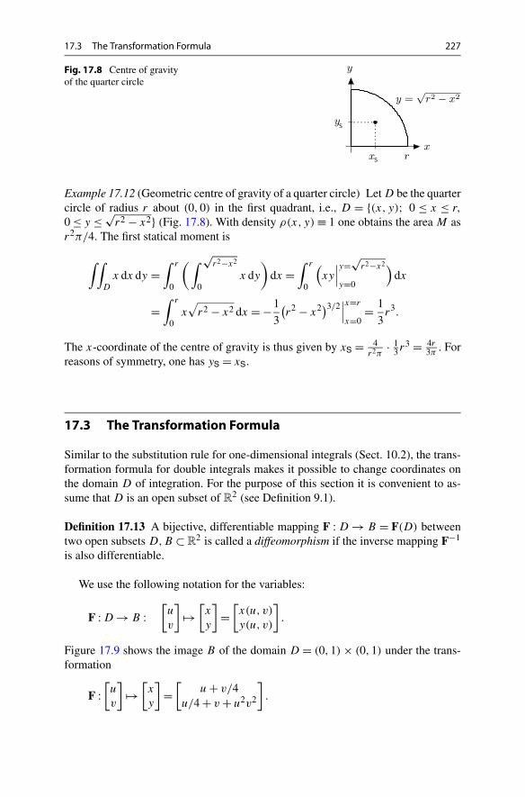
17.3 The Transformation Formula 227
Fig. 17.8 Centre of gravityof the quarter circle
Example 17.12 (Geometric centre of gravity of a quarter circle) Let D be the quartercircle of radius r about (0,0) in the first quadrant, i.e., D = {(x, y); 0 ≤ x ≤ r,
0 ≤ y ≤ √r2 − x2} (Fig. 17.8). With density ρ(x, y) ≡ 1 one obtains the area M as
r2π/4. The first statical moment is
∫ ∫D
x dx dy =∫ r
0
(∫ √r2−x2
0x dy
)dx =
∫ r
0
(xy
∣∣∣y=√
r2−x2
y=0
)dx
=∫ r
0x√
r2 − x2 dx = −1
3
(r2 − x2)3/2
∣∣∣x=r
x=0= 1
3r3.
The x-coordinate of the centre of gravity is thus given by xS = 4r2π
· 13 r3 = 4r
3π. For
reasons of symmetry, one has yS = xS.
17.3 The Transformation Formula
Similar to the substitution rule for one-dimensional integrals (Sect. 10.2), the trans-formation formula for double integrals makes it possible to change coordinates onthe domain D of integration. For the purpose of this section it is convenient to as-sume that D is an open subset of R
2 (see Definition 9.1).
Definition 17.13 A bijective, differentiable mapping F : D → B = F(D) betweentwo open subsets D,B ⊂ R
2 is called a diffeomorphism if the inverse mapping F−1
is also differentiable.
We use the following notation for the variables:
F : D → B :[u
v
]�→
[x
y
]=
[x(u, v)
y(u, v)
].
Figure 17.9 shows the image B of the domain D = (0,1) × (0,1) under the trans-formation
F :[u
v
]�→
[x
y
]=
[u + v/4
u/4 + v + u2v2
].

228 17 Integration of Functions of Two Variables
Fig. 17.9 Transformation ofa planar domain
The aim is to transform the integral of a real-valued function f over the domain B
to one over D.For this purpose we lay a grid G over the domain D in the (u, v)-plane and select
a rectangle, for instance with the left lower corner (u, v) and sides spanned by thevectors[
�u0
],
[0
�v
].
The image of this rectangle under the transformation F will in general have a curvi-linear boundary. In a first approximation we replace it by a parallelogram. In linearapproximation (see Sect. 15.4) we have
F(u + �u,v) ≈ F(u, v) + F′(u, v)
[�u0
],
F(u, v + �v) ≈ F(u, v) + F′(u, v)
[0
�v
].
The approximating parallelogram is thus spanned by the vectors
[∂x∂u
(u, v)
∂y∂u
(u, v)
]�u,
[∂x∂v
(u, v)
∂y∂v
(u, v)
]�v,
and it has the area (see Sect. 22.5)∣∣∣∣∣det
[∂x∂u
(u, v) ∂x∂v
(u, v)
∂y∂u
(u, v)∂y∂v
(u, v)
]�u�v
∣∣∣∣∣ = ∣∣det F′(u, v)∣∣�u�v.
In short, the area element �A = �u�v is changed by the transformation F to thearea element �F(A) = |det F′(u, v)|�u�v (see Fig. 17.10).
Proposition 17.14 (Transformation formula for double integrals) Let D, B beopen, bounded subsets of R
2, F : D → B a diffeomorphism and f : B → R abounded mapping. Then
∫ ∫B
f (x, y)dx dy =∫ ∫
D
f(F(u, v)
)∣∣det F′(u, v)∣∣dudv,
as long as the functions f and f (F)|det F′| are Riemann integrable.


230 17 Integration of Functions of Two Variables
Its volume is obtained by integration of the function f (x, y) = √R2 − x2 − y2 over
the base B = {(x, y); 0 ≤ x2 + y2 ≤ R2}. In polar coordinates
F : R2 → R
2 :[rϕ
]�→
[xy
]=
[r cosϕr sinϕ
]
the area B can be represented as the image F(D) of the rectangle D = [0,R] ×[0,2π]. However, in order to fulfill the assumptions of Proposition 17.14 we haveto switch to open domains on which F is a diffeomorphism. We can obtain this, forinstance, by removing the boundary and the half ray {(x, y); 0 ≤ x ≤ R, y = 0} ofthe circle B and the boundary of the rectangle D. On the smaller domains D′ and B ′obtained in this way, F is a diffeomorphism. However, since B differs from B ′ andD differs from D′ by sets of measure zero, the value of the integral is not changedif one replaces B by B ′ and D by D′; see Remark 17.6. We have
F′(r, ϕ) =[
cosϕ −r sinϕsinϕ r cosϕ
],
∣∣det F′(r, ϕ)∣∣ = r.
Substituting x = r cosϕ, y = r sinϕ results in x2 + y2 = r2, and we obtain thevolume from the transformation formula:
∫ ∫B
√R2 − x2 − y2 dx dy =
∫ R
0
∫ 2π
0
√R2 − r2r dϕ dr
=∫ R
02πr
√R2 − r2 dr
= −2π
3
(R2 − r2)3/2
∣∣∣r=R
r=0= 2π
3R3,
which coincides with the known result from elementary geometry.
17.4 Exercises
1. Compute the volume of the parabolic dome z = 2 − x2 − y2 above the quadraticdomain D : −1 ≤ x ≤ 1, −1 ≤ y ≤ 1.
2. (From statics) Compute the axial moment of inertia∫∫
Dy2 dx dy of a rectangular
cross section D : 0 ≤ x ≤ b, −h/2 ≤ y ≤ h/2, where b > 0, h > 0.3. Compute the volume of the body bounded by the plane z = x + y above the
domain D : 0 ≤ x ≤ 1,0 ≤ y ≤ √1 − x2.
4. Compute the volume of the body bounded by the plane z = 6 − x − y abovethe domain D, which is bounded by the y-axis and the straight lines x + y = 6,x + 3y = 6 (x ≥ 0, y ≥ 0).
5. Compute the geometric centre of gravity of the domain D : 0 ≤ x ≤ 1,0 ≤ y ≤1 − x2.

17.4 Exercises 231
6. Compute the area and the geometric centre of gravity of the semi-ellipse
x2
a2+ y2
b2≤ 1, y ≥ 0.
Hint. Introduce elliptic coordinates x = ar cosϕ, y = br sinϕ, 0 ≤ r ≤ 1, 0 ≤ϕ ≤ π , compute the Jacobian and use the transformation formula.
7. (From statics) Compute the axial moment of inertia of a ring with inner radiusR1 and outer radius R2 with respect to the central axis, i.e., the integral
∫∫D
(x2 +y2)dx dy over the domain D : R1 ≤ √
x2 + y2 ≤ R2.8. Modify the M-file mat17_1.m so that it can evaluate Riemann sums over equi-
distant partitions with �x �= �y.

18Linear Regression
Linear regression is one of the most important methods of data analysis. It servesthe determination of model parameters, model fitting, assessing the importance ofinfluencing factors, and prediction, in all areas of human, natural and economicsciences. Computer scientists who work closely with people from these areas willdefinitely come across regression models.
The aim of this chapter is a first introduction into the subject. We deduce the co-efficients of the regression models using the method of least squares to minimise theerrors. We will only employ methods of descriptive data analysis. We do not touchupon the more advanced probabilistic approaches which are topics of statistics. Forall that, as well as for nonlinear regression, we refer to the specialised literature.
We start with simple (or univariate) linear regression—a model with a single in-put and a single output quantity—and explain the basic ideas of analysis of variancefor model evaluation. Then we turn to multiple (or multivariate) linear regressionwith several input quantities. The chapter closes with a descriptive approach to de-termine the influence of the individual coefficients.
18.1 Simple Linear Regression
A first glance at the basic idea of linear regression was already given in Sect. 8.3. Inextension to this, we will now allow for more general models, in particular regres-sion lines with nonzero intercept.
Consider pairs of data (x1, y1), . . . , (xn, yn), obtained as observations or mea-surements. Geometrically they form a scatter plot in the plane. The values xi and yi
may appear repeatedly in this list of data. In particular, for a given xi there may bedata points with different values yi1, . . . , yip . The general task of linear regressionis to fit the graph of a function
y = β0ϕ0(x) + β1ϕ1(x) + · · · + βmϕm(x)
M. Oberguggenberger, A. Ostermann, Analysis for Computer Scientists,Undergraduate Topics in Computer Science,DOI 10.1007/978-0-85729-446-3_18, © Springer-Verlag London Limited 2011
233


18.1 Simple Linear Regression 235
Fig. 18.2 Scatter plot heightof fathers/height of the sons,regression line
Formally, this problem is identical to the standard problem of linear regression,however, with transformed data:
(ξi, ηi) = (ϕ(xi),ψ(yi)
).
A typical example is given by the loglinear regression with ξ = logx, η = logy
logy = β0 + β1 logx,
which in the original variables amounts to the approach
y = eβ0xβ1 .
If the variable x itself has several components which enter linearly in the model,then one speaks of multiple linear regression. We will deal with it in Sect. 18.3.
The notion of regression was introduced by Galton,1 who observed, while inves-tigating the height of sons/fathers, a tendency of regressing to the average size. Thedata taken from [14] clearly show this effect; see Fig. 18.2. The method of leastsquares goes back to Gauss.
After these introductory remarks about the general concept of linear regression,we turn to a simple linear regression. We start with setting up the model. The pos-tulated relationship between x and y is linear
y = β0 + β1x
with unknown coefficients β0 and β1. In general, the given data will not exactly lieon a straight line but deviate by εi , i.e.,
yi = β0 + β1xi + εi,
as represented in Fig. 18.3.From the given data we want to obtain estimated values β0, β1 for β0, β1. This is
achieved through minimising the sum of squares of the errors
L(β0, β1) =n∑
i=1
ε2i =
n∑i=1
(yi − β0 − β1xi)2,
1F. Galton, 1822–1911.
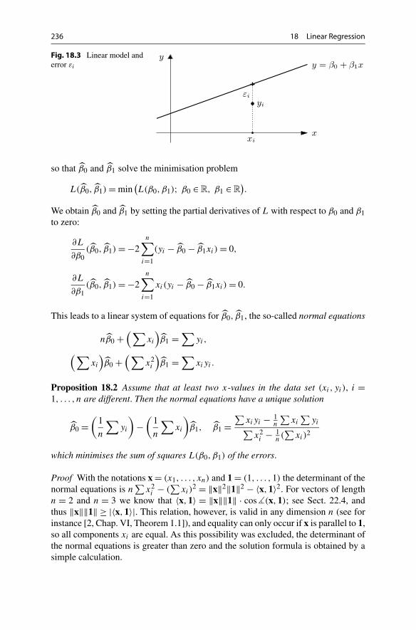
236 18 Linear Regression
Fig. 18.3 Linear model anderror εi
so that β0 and β1 solve the minimisation problem
L(β0, β1) = min(L(β0, β1); β0 ∈ R, β1 ∈ R
).
We obtain β0 and β1 by setting the partial derivatives of L with respect to β0 and β1to zero:
∂L
∂β0(β0, β1) = −2
n∑i=1
(yi − β0 − β1xi) = 0,
∂L
∂β1(β0, β1) = −2
n∑i=1
xi(yi − β0 − β1xi) = 0.
This leads to a linear system of equations for β0, β1, the so-called normal equations
nβ0 +(∑
xi
)β1 =
∑yi,
(∑xi
)β0 +
(∑x2i
)β1 =
∑xiyi .
Proposition 18.2 Assume that at least two x-values in the data set (xi, yi), i =1, . . . , n are different. Then the normal equations have a unique solution
β0 =(
1
n
∑yi
)−
(1
n
∑xi
)β1, β1 =
∑xiyi − 1
n
∑xi
∑yi∑
x2i − 1
n(∑
xi)2
which minimises the sum of squares L(β0, β1) of the errors.
Proof With the notations x = (x1, . . . , xn) and 1 = (1, . . . ,1) the determinant of thenormal equations is n
∑x2i − (
∑xi)
2 = ‖x‖2‖1‖2 − 〈x,1〉2. For vectors of lengthn = 2 and n = 3 we know that 〈x,1〉 = ‖x‖‖1‖ · cos�(x,1); see Sect. 22.4, andthus ‖x‖‖1‖ ≥ |〈x,1〉|. This relation, however, is valid in any dimension n (see forinstance [2, Chap. VI, Theorem 1.1]), and equality can only occur if x is parallel to 1,so all components xi are equal. As this possibility was excluded, the determinant ofthe normal equations is greater than zero and the solution formula is obtained by asimple calculation.

18.1 Simple Linear Regression 237
Fig. 18.4 Linear model,prediction, residual
In order to show that this solution minimises L(β0, β1), we compute the Hessianmatrix
HL =⎡⎣
∂2L
∂β20
∂2L∂β0∂β1
∂2L∂β1∂β0
∂2L
∂β21
⎤⎦ = 2
[n
∑xi∑
xi
∑x2i
]= 2
[ ‖1‖2 〈x,1〉〈x,1〉 ‖x‖2
].
The entry ∂2L/∂β20 = 2n and detHL = 4(‖x‖2‖1‖2 −〈x,1〉2) are both positive. Ac-
cording to Proposition 15.28, L has an isolated local minimum at the point (β0, β1).Due to the uniqueness of the solution, this is the only minimum of L. �
The assumption that there are at least two different xi -values in the data set is nota restriction, since otherwise the regression problem is not meaningful. The resultof the regression is the predicted regression line
y = β0 + β1x.
The values predicted by the model are then
yi = β0 + β1xi, i = 1, . . . , n.
Their deviations from the data values yi are called residuals
ei = yi − yi = yi − β0 − β1xi, i = 1, . . . , n.
The meaning of these quantities can be seen in Fig. 18.4.With the above specifications, the deterministic regression model is completed. In
the statistical regression model the errors εi are interpreted as random variables withmean zero. Under further probabilistic assumptions, the model is made accessible tostatistical tests and diagnostic procedures. As mentioned in the introduction, we willnot pursue this path here but remain in the framework of descriptive data analysis.
In order to obtain a more lucid representation, we will reformulate the normalequations. For this, we introduce the following vectors and matrices:
y =
⎡⎢⎢⎢⎣
y1y2...
yn
⎤⎥⎥⎥⎦ , X =
⎡⎢⎢⎢⎣
1 x11 x2...
...
1 xn
⎤⎥⎥⎥⎦ , β =
[β0β1
], ε =
⎡⎢⎢⎢⎣
ε1ε2...
εn
⎤⎥⎥⎥⎦ .
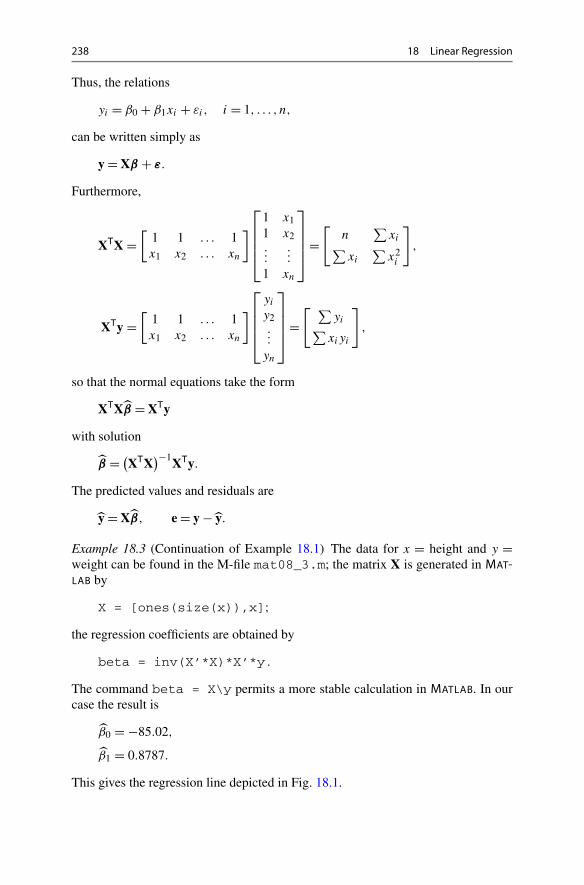
238 18 Linear Regression
Thus, the relations
yi = β0 + β1xi + εi, i = 1, . . . , n,
can be written simply as
y = Xβ + ε.
Furthermore,
XTX =[
1 1 . . . 1x1 x2 . . . xn
]⎡⎢⎢⎢⎣
1 x11 x2...
...
1 xn
⎤⎥⎥⎥⎦ =
[n
∑xi∑
xi
∑x2i
],
XTy =[
1 1 . . . 1x1 x2 . . . xn
]⎡⎢⎢⎢⎣
yi
y2...
yn
⎤⎥⎥⎥⎦ =
[ ∑yi∑
xiyi
],
so that the normal equations take the form
XTXβ = XTy
with solution
β = (XTX
)−1XTy.
The predicted values and residuals are
y = Xβ, e = y − y.
Example 18.3 (Continuation of Example 18.1) The data for x = height and y =weight can be found in the M-file mat08_3.m; the matrix X is generated in MAT-LAB by
X = [ones(size(x)),x];the regression coefficients are obtained by
beta = inv(X’*X)*X’*y .
The command beta = X\y permits a more stable calculation in MATLAB. In ourcase the result is
β0 = −85.02,
β1 = 0.8787.
This gives the regression line depicted in Fig. 18.1.

18.2 Rudiments of the Analysis of Variance 239
18.2 Rudiments of the Analysis of Variance
First indications for the quality of fit of the linear model can be obtained from theanalysis of variance (ANOVA), which also forms the basis for more advanced sta-tistical test procedures.
The arithmetic mean of the y-values y1, . . . , yn is
y = 1
n
n∑i=1
yi .
The deviation of the measured value yi from the mean value y is yi − y. The totalsum of squares or total variability of the data is
Syy =n∑
i=1
(yi − y)2.
The total variability is split into two components in the following way:
n∑i=1
(yi − y)2 =n∑
i=1
(yi − y)2 +n∑
i=1
(yi − yi )2.
The validity of this relationship will be proven in Proposition 18.4 below. It is in-terpreted as follows: yi − y is the deviation of the predicted value from the meanvalue, and
SSR =n∑
i=1
(yi − y)2
the regression sum of squares. This is interpreted as the part of the data variabilityaccounted for by the model. On the other hand ei = yi − yi are the residuals, and
SSE =n∑
i=1
(yi − yi )2
is the error sum of squares, which is interpreted as the part of the variability thatremains unexplained by the linear model. These notions are best explained by con-sidering the two extremal cases.(a) The data values yi themselves already lie on a straight line. Then all yi = yi and
thus Syy = SSR, SSE = 0, and the regression model describes the data recordexactly.
(b) The data values are in no linear relation. Then the line of best fit is the horizontalline through the mean value (see Exercise 12 of Chap. 8), so yi = y for all i andhence Syy = SSE, SSR = 0. This means that the regression model does not offerany indication for a linear relation between the values.
240 18 Linear Regression
The basis of these considerations is the validity of the following formula.
Proposition 18.4 (Partitioning of total variability) Syy = SSR + SSE.
Proof In the following, we use matrix and vector notation. In particular, we employthe formulae
aTb = bTa =∑
aibi, 1Ta = aT1 =∑
ai = na, aTa =∑
a2i
for vectors a,b, and the matrix identity (AB)T = BTAT. We have
Syy = (y − y1)T(y − y1) = yTy − y(1Ty
) − (yT1
)y + ny2
= yTy − ny2 − ny2 + ny2 = yTy − ny2,
SSE = eTe = (y − y)T(y − y ) = (y − Xβ)T(y − Xβ)
= yTy − βTXTy − yTXβ + β
TXTXβ = yTy − β
TXTy.
For the last equality we have used the normal equations XTXβ = XTy and the trans-
position formula βTXTy = (yTXβ)T = yTXβ . The relation y = Xβ implies, in par-
ticular, XTy = XTy. Since the first line of XT consists of ones only, it follows that1Ty = 1Ty and thus
SSR = (y − y1)T(y − y1) = yTy − y(1Ty
) − (yT1
)y + ny2
= yTy − ny2 − ny2 + ny2 = βT(
XTXβ) − ny2 = β
TXTy − ny2.
Summation of the obtained expressions for SSE and SSR results in the sought-afterformula. �
The partitioning of total variability
Syy = SSR + SSE
and its above interpretation suggest using the quantity
R2 = SSR
Syy
for the assessment of the goodness of fit. The quantity R2 is called the coefficient ofdetermination and measures the fraction of variability explained by the regression.In the limiting case of an exact fit, where the regression line passes through all datapoints, we have SSE = 0 and thus R2 = 1. A small value of R2 indicates that thelinear model does not fit the data.
Remark 18.5 An essential point in the proof of Proposition 18.4 was the propertyof XT that its first line was composed of ones only. This is a consequence of thefact that β0 was a model parameter. In the regression where a straight line through

18.2 Rudiments of the Analysis of Variance 241
the origin is used (see Sect. 8.3) this is not the case. For a regression which doesnot have β0 as a parameter, the variance partition is not valid and the coefficient ofdetermination is meaningless.
Example 18.6 We continue the investigation of the relation between height andweight from Example 18.1. Using the MATLAB program mat18_1.m and enteringthe data from mat08_3.m results in
Syy = 9584.9, SSE = 8094.4, SSR = 1490.5
and
R2 = 0.1555, R = 0.3943.
The low value of R2 is a clear indication that height and weight are not in a linearrelation.
Example 18.7 In Sect. 9.1 the fractal dimension d = d(A) of a bounded subset A
of R2 was defined by the limit
d = d(A) = − limε→0+ logN(A,ε)/ log ε,
where N(A,ε) denoted the smallest number of squares of side length ε needed tocover A. For the experimental determination of the dimension of a fractal set A,one rasters the plane with different mesh sizes ε and determines the number N =N(A,ε) of boxes that have a non-empty intersection with the fractal. As explainedin Sect. 9.1, one uses the approximation
N(A,ε) ≈ C · ε−d .
Applying logarithms results in
logN(A,ε) ≈ logC + d log1
ε,
which is a linear model,
y ≈ β0 + β1x,
for the quantities x = log 1/ε, y = logN(A,ε). The regression coefficient β1 canbe used as an estimate for the fractal dimension d .
In Exercise 1 of Sect. 9.6 this procedure was applied to the coastline of GreatBritain. Assume that the following values were obtained:
1/ε 4 8 12 16 24 32N(A,ε) 16 48 90 120 192 283

242 18 Linear Regression
Fig. 18.5 Fractal dimensionof the coast line of GreatBritain
A linear regression through the logarithms x = log 1/ε, y = logN(A,ε) yields thecoefficients
β0 = 0.9849, d ≈ β1 = 1.3616,
with the coefficient of determination
R2 = 0.9930.
This is very good fit, which is also confirmed by Fig. 18.5. The given data thusindicate that the fractal dimension of the coast line of Great Britain is d = 1.36.
A word of caution is in order. Data analysis can only supply indications, but nevera proof that a model is correct. Even if we choose among a number of wrong modelsthe one with the largest R2, this model will not become correct. A healthy amount ofscepticism with respect to purely empirically inferred relations is advisable; modelsshould always be critically questioned. Scientific progress arises from the interplaybetween the invention of models and their experimental validation through data.
18.3 Multiple Linear Regression
In multiple (multivariate) linear regression the variable y does not just depend onone regressor variable x, but on several variables, for instance x1, x2, . . . , xk . Weemphasise that the notation with respect to Sect. 18.1 is changed—there xi denotedthe ith data value, now xi refers to the ith regressor variable. The measurements ofthe ith regressor variable are now denoted with two indices, namely xi1, xi2, . . . , xin.In total, there are k × n data values. We again look for a linear model,
y = β0 + β1x1 + β2x2 + · · · + βkxk,
with the yet unknown coefficients β0, β1, . . . , βk .
Example 18.8 A vending machine company wants to analyse the delivery time,i.e., the time span y which a driver needs to refill a machine. The most im-portant parameters are the number x1 of refilled product units and the distancex2 walked by the driver. The results of an observation of 25 services are given
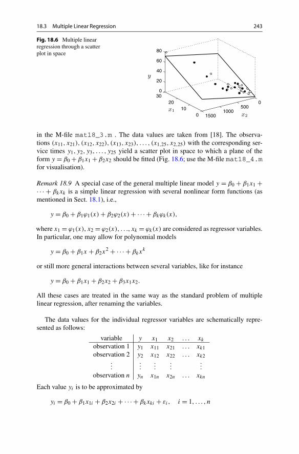
18.3 Multiple Linear Regression 243
Fig. 18.6 Multiple linearregression through a scatterplot in space
in the M-file mat18_3.m . The data values are taken from [18]. The observa-tions (x11, x21), (x12, x22), (x13, x23), . . . , (x1,25, x2,25) with the corresponding ser-vice times y1, y2, y3, . . . , y25 yield a scatter plot in space to which a plane of theform y = β0 + β1x1 + β2x2 should be fitted (Fig. 18.6; use the M-file mat18_4.mfor visualisation).
Remark 18.9 A special case of the general multiple linear model y = β0 + β1x1 +· · · + βkxk is a simple linear regression with several nonlinear form functions (asmentioned in Sect. 18.1), i.e.,
y = β0 + β1ϕ1(x) + β2ϕ2(x) + · · · + βkϕk(x),
where x1 = ϕ1(x), x2 = ϕ2(x), . . ., xk = ϕk(x) are considered as regressor variables.In particular, one may allow for polynomial models
y = β0 + β1x + β2x2 + · · · + βkx
k
or still more general interactions between several variables, like for instance
y = β0 + β1x1 + β2x2 + β3x1x2.
All these cases are treated in the same way as the standard problem of multiplelinear regression, after renaming the variables.
The data values for the individual regressor variables are schematically repre-sented as follows:
variable y x1 x2 . . . xk
observation 1 y1 x11 x21 . . . xk1observation 2 y2 x12 x22 . . . xk2
......
......
...
observation n yn x1n x2n . . . xkn
Each value yi is to be approximated by
yi = β0 + β1x1i + β2x2i + · · · + βkxki + εi, i = 1, . . . , n
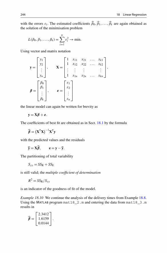
244 18 Linear Regression
with the errors εi . The estimated coefficients β0, β1, . . . , βk are again obtained asthe solution of the minimisation problem
L(β0, β1, . . . , βk) =n∑
i=1
ε2i → min.
Using vector and matrix notation
y =
⎡⎢⎢⎢⎣
y1y2...
yn
⎤⎥⎥⎥⎦ , X =
⎡⎢⎢⎢⎣
1 x11 x21 . . . xk11 x12 x22 . . . xk2...
......
...
1 x1n x2n . . . xkn
⎤⎥⎥⎥⎦ ,
β =
⎡⎢⎢⎢⎣
β0β1...
βk
⎤⎥⎥⎥⎦ , ε =
⎡⎢⎢⎢⎣
ε1ε2...
εn
⎤⎥⎥⎥⎦
the linear model can again be written for brevity as
y = Xβ + ε.
The coefficients of best fit are obtained as in Sect. 18.1 by the formula
β = (XTX
)−1XTy
with the predicted values and the residuals
y = Xβ, e = y − y.
The partitioning of total variability
Syy = SSR + SSE
is still valid; the multiple coefficient of determination
R2 = SSR/Syy
is an indicator of the goodness of fit of the model.
Example 18.10 We continue the analysis of the delivery times from Example 18.8.Using the MATLAB program mat18_2.m and entering the data from mat18_3.mresults in
β =⎡⎣2.3412
1.61590.0144
⎤⎦ .

18.4 Model Fitting and Variable Selection 245
We obtain the model
y = 2.3412 + 1.6159x1 + 0.0144x2
with the multiple coefficient of determination of
R2 = 0.9596
and the partitioning of total variability
Syy = 5784.5, SSR = 5550.8, SSE = 233.7.
In this example merely (1 − R2) · 100% ≈ 4% of the variability of the data is notexplained by the regression, a very satisfactory goodness of fit.
18.4 Model Fitting and Variable Selection
A recurring problem is to decide which variables should be included in the model.Would the inclusion of x3 = x2
2 and x4 = x1x2, i.e., the model
y = β0 + β1x1 + β2x2 + β3x22 + β4x1x2,
lead to better results, and can, e.g., the term β2x2 be eliminated subsequently? It isnot desirable to have too many variables in the model. If there are as many variablesas data points, then one can fit the regression exactly through the data and the modelwould loose its predictive power. A criterion will definitely be to reach a value of R2
which is as large as possible. Another aim is to eliminate variables that do not con-tribute essentially to the total variability. An algorithmic procedure for identifyingthese variables is the sequential partitioning of total variability.
Sequential Partitioning of Total Variability We include variables stepwise in themodel, thus consider the increasing sequence of models with corresponding SSR:
y = β0 SSR(β0),
y = β0 + β1x1 SSR(β0, β1),
y = β0 + β1x1 + β2x2 SSR(β0, β1, β2),
......
y = β0 + β1x1 + β2x2 + · · · + βkxk SSR(β0, β1, . . . , βk) = SSR.
Note that SSR(β0) = 0, since in the initial model β0 = y. The additional explana-tory power of the variable x1 is measured by
SSR(β1|β0) = SSR(β0, β1) − 0,

246 18 Linear Regression
the power of variable x2 (if x1 is already in the model) by
SSR(β2|β0, β1) = SSR(β0, β1, β2) − SSR(β0, β1),
the power of variable xk (if x1, x2, . . . , xk−1 are in the model) by
SSR(βk|β0, β1, . . . , βk−1) = SSR(β0, β1, . . . , βk) − SSR(β0, β1, . . . , βk−1).
Obviously,
SSR(β1|β0) + SSR(β2|β0, β1) + SSR(β3|β0, β1, β2) + · · ·+ SSR(βk|β0, β1, β2, . . . , βk−1) = SSR.
This shows that one can interpret the sequential, partial coefficient of determination
SSR(βj |β0, β1, . . . , βj−1)
Syy
as explanatory power of the variables xj , under the condition that the variablesx1, x2, . . . , xj−1 are already included in the model. This partial coefficient of de-termination depends on the order of the added variables. This dependency can beeliminated by averaging over all possible sequences of variables.
Average Explanatory Power of Individual Coefficients One first computes allpossible sequential, partial coefficients of determination which can be obtained byadding the variable xj to all possible combinations of the already included vari-ables. Summing up these coefficients and dividing the result by the total numberof possibilities, one obtains a measure for the contribution of the variable xj to theexplanatory power of the model.
Average over orderings was proposed by [15]; further details and advanced con-siderations can be found, for instance, in [8, 10]. The concept does not use prob-abilistically motivated indicators. Instead, it is based on the data and on combina-torics, and thus it belongs to descriptive data analysis. Such descriptive methods,in contrast to the commonly used statistical hypothesis testing, do not require addi-tional assumptions, which may be difficult to justify.
Example 18.11 We compute the explanatory power of the coefficients in the deliv-ery time problem of Example 18.8. First we fit the two univariate models
y = β0 + β1x1, y = β0 + β2x2
and from that obtain
SSR(β0, β1) = 5382.4, SSR(β0, β2) = 4599.1,


248 18 Linear Regression
values of SSR.
1 2 3 SSR(β1|β0) SSR(β2|β0, β1) SSR(β3|β0, β1, β2)
1 3 2 SSR(β1|β0) SSR(β3|β0, β1) SSR(β2|β0, β1, β3)
2 1 3 SSR(β2|β0) SSR(β1|β0, β2) SSR(β3|β0, β2, β1)
2 3 1 SSR(β2|β0) SSR(β3|β0, β2) SSR(β1|β0, β2, β3)
3 1 2 SSR(β3|β0) SSR(β1|β0, β3) SSR(β2|β0, β3, β1)
3 2 1 SSR(β3|β0) SSR(β2|β0, β3) SSR(β1|β0, β3, β2)
Obviously the sum of each row is always equal to SSR, so that the sum of all entriesis equal to 6 · SSR. Note that amongst the 18 SSR-values there are actually only 12different ones.
The average explanatory power of the variable x1 is defined by M1/Syy , where
M1 = 1
6
(SSR(β1|β0) + SSR(β1|β0) + SSR(β1|β0, β2) + SSR(β1|β0, β3)
+ SSR(β1|β0, β2, β3) + SSR(β1|β0, β3, β2))
and analogously for the other variables. As remarked above, we have
M1 + M2 + M3 = SSR,
and thus the total partitioning adds up to 1:
M1
Syy
+ M2
Syy
+ M3
Syy
+ SSE
Syy
= 1.
For a more detailed analysis of the underlying combinatorics, for the necessary mod-ifications in the case of collinearity of the data (linear dependence of the columnsof the matrix X) and for a discussion of the significance of the average explanatorypower, we refer to the literature quoted above. The algorithm is implemented in theapplet Linear regression.
Experiment 18.12 Open the applet Linear regression and load Data set number 9.It contains experimental data quantifying the influence of different aggregates ona mixture of concrete. The meaning of the output variables x1 through x4 and theinput variables x5 through x13 is explained in the online description of the applet.Experiment with different selections of the variables of the model. An interestinginitial model is obtained, for example, by choosing x6, x8, x9, x10, x11, x12, x13 asindependent and x1 as dependent variable; then remove variables with a low ex-planatory power and draw a pie chart.

18.5 Exercises 249
18.5 Exercises
1. The total consumption of electric energy in Austria in the years 1975–2005 isgiven in the table below (from [24, Table 22.13]). The task is to carry out a linearregression of the form y = β0 + β1x through the data.(a) Write down the matrix X explicitly and compute the coefficients β =
[β0, β1]T using the MATLAB command beta = X\y.(b) Check the goodness of fit by computing R2. Plot a scatter diagram with the
fitted straight line. Compute the forecast y for 2010.
year xi 1975 1980 1985 1990 1995 2000 2005consumption yi [GWh] 30.663 37.995 42.815 49.951 54.177 60.502 65.199
2. A sample of n = 44 civil engineering students at the University of Innsbruck inthe year 1998 gave the values for x = height [cm] and y = weight [kg] listed inthe M-file mat18_ex2.m. Compute the regression line y = β0 + β1x, plot thescatter diagram and calculate the coefficient of determination R2.
3. Solve Exercise 1 using Excel.4. Solve Exercise 1 using the statistics package SPSS.
Hint. Enter the data in the worksheet Data View; the names of the variables andtheir properties can be defined in the worksheet Variable View. Go to Analyze →Regression → Linear.
5. The stock of buildings in Austria in the years 1869–2001 is given in the M-filemat18_ex5.m (data from [24]). Compute the regression line y = β0 +β1x andthe regression parabola y = α0 + α1(x − 1860)2 through the data and test whichmodel fits better, using the coefficient of determination R2.
6. The monthly share index for four breweries from November 1999 to November2000 is given in the M-file mat18_ex6.m (November 1999 = 100%, from theAustrian magazine profil 46/2000). Fit a univariate linear model y = β0 + β1x
to each of the four data sets (x is for date, y is for share index), plot the resultsin four equally scaled windows, evaluate the results by computing R2 and checkwhether the caption provided by profil is justified by the data. For the calculationyou may use the MATLAB program mat18_1.m.Hint. A solution is suggested in the M-file mat18_exsol6.m.
7. Continuation of Exercise 5, stock of buildings in Austria. Fit the model
y = β0 + β1x + β2(x − 1860)2
and compute SSR = SSR(β0, β1, β2) and Syy . Further, analyse the increase ofexplanatory power through adding the respective missing variable in the modelsof Exercise 5, i.e., compute SSR(β2|β0, β1) and SSR(β1|β0, β2) as well as theaverage explanatory power of the individual coefficients. Compare with the resultfor Data set number 5 in the applet Linear regression.
8. The M-file mat18_ex8.m contains the mileage per gallon y of 30 cars depend-ing on the engine displacement x1, the horsepower x2, the overall length x3 andthe weight x4 of the vehicle (from: Motor Trend 1975, according to [18]). Fit the
250 18 Linear Regression
linear model
y = β0 + β1x1 + β2x2 + β3x3 + β4x4,
and estimate the explanatory power of the individual coefficients through a sim-ple sequential analysis:
SSR(β1|β0), SSR(β2|β0, β1), SSR(β3|β0, β1, β2),
SSR(β4|β0, β1, β2, β3).
Compare your result with the average explanatory power of the coefficients forData set number 2 in the applet Linear regression.Hint. A suggested solution is given in the M-file mat18_exsol8.m.
9. Check the results of Exercises 1, 2 and 6 using the applet Linear regression (Datasets 6, 1 and 4); likewise for the Examples 18.1 and 18.8 with Data sets 8 and 3.In particular, investigate in Data set 8 whether height, weight and the risk ofbreaking a leg are in any linear relation.
19Differential Equations
In this chapter we discuss the theory of initial value problems for ordinary differen-tial equations. We limit ourselves to scalar equations here; systems will be discussedin the next chapter.
After presenting the general definition of a differential equation and the geomet-ric significance of its direction field, we start with a detailed discussion of first-orderlinear equations. As important applications we discuss the modelling of growth anddecay processes. Subsequently, we investigate questions of existence and (local)uniqueness of the solution of general differential equations and discuss the methodof power series. Finally, we study the qualitative behaviour of solutions close to anequilibrium point.
19.1 Initial Value Problems
Differential equations are equations involving a (sought after) function and itsderivative(s). They play a decisive role in modelling time dependent processes.
Definition 19.1 Let D ⊂ R2 be open and f : D ⊂ R
2 → R continuous. The equa-tion
y′(x) = f(x, y(x)
)is called (an ordinary) first-order differential equation. A solution is a differentiablefunction y : I → D which satisfies the equation for all x ∈ I .
One often suppresses the independent variable x in the notation and writes theabove problem for brevity as
y′ = f (x, y).
The sought-after function y in this equation is also called the dependent variable(depending on x).
M. Oberguggenberger, A. Ostermann, Analysis for Computer Scientists,Undergraduate Topics in Computer Science,DOI 10.1007/978-0-85729-446-3_19, © Springer-Verlag London Limited 2011
251
252 19 Differential Equations
In modelling time dependent processes, one usually denotes the independentvariable by t (for time) and the dependent variable by x = x(t). In this case onewrites the first-order differential equation as
x(t) = f(t, x(t)
)or for short as x = f (t, x).
Example 19.2 (Separation of the variables) We want to find all functions y = y(x)
satisfying the equation y′(x) = x · y(x)2. In this example one obtains the solutionsby separating the variables. For y �= 0 one divides the differential equation by y2
and gets
1
y2· y′ = x.
The left-hand side of this equation is of the form g(y) ·y′. Let G(y) be an antideriva-tive of g(y). According to the chain rule, and recalling that y is a function of x, weobtain
d
dxG(y) = d
dyG(y) · dy
dx= g(y) · y′.
In our example we have g(y) = y−2 and G(y) = −y−1, consequently
d
dx
(− 1
y
)= 1
y2· y′ = x.
Integration of this equation with respect to x results in
− 1
y= x2
2+ C,
where C denotes an arbitrary integration constant. By elementary manipulations wefind
y = 1
−x2/2 − C= 2
K − x2
with the constant K = −2C.The function y = 0 is also a solution of the differential equation. Formally, one
obtains it from the above solution by setting K = ∞. The example shows that dif-ferential equations have infinitely many solutions in general. By requiring an addi-tional condition, a unique solution can be selected. For example, setting y(0) = 1gives y(x) = 2/(2 − x2).
Definition 19.3 The differential equation y′(x) = f (x, y(x)) together with the ad-ditional condition y(x0) = y0, i.e.,
y′(x) = f(x, y(x)
), y(x0) = y0,
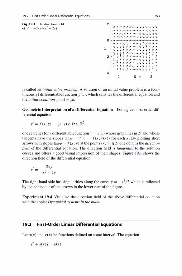
19.2 First-Order Linear Differential Equations 253
Fig. 19.1 The direction fieldof y′ = −2xy/(x2 + 2y)
is called an initial value problem. A solution of an initial value problem is a (con-tinuously) differentiable function y(x), which satisfies the differential equation andthe initial condition y(x0) = y0.
Geometric Interpretation of a Differential Equation For a given first-order dif-ferential equation
y′ = f (x, y), (x, y) ∈ D ⊂ R2
one searches for a differentiable function y = y(x) whose graph lies in D and whosetangents have the slopes tanϕ = y′(x) = f (x, y(x)) for each x. By plotting shortarrows with slopes tanϕ = f (x, y) at the points (x, y) ∈ D one obtains the directionfield of the differential equation. The direction field is tangential to the solutioncurves and offers a good visual impression of their shapes. Figure 19.1 shows thedirection field of the differential equation
y′ = − 2xy
x2 + 2y.
The right-hand side has singularities along the curve y = −x2/2 which is reflectedby the behaviour of the arrows in the lower part of the figure.
Experiment 19.4 Visualise the direction field of the above differential equationwith the applet Dynamical systems in the plane.
19.2 First-Order Linear Differential Equations
Let a(x) and g(x) be functions defined on some interval. The equation
y′ + a(x)y = g(x)

254 19 Differential Equations
is called a first-order linear differential equation. The function a is the coefficient,the right-hand side g is called an inhomogeneity. The differential equation is calledhomogeneous, if g = 0; otherwise inhomogeneous. First we state the following im-portant result.
Proposition 19.5 (Superposition principle) If y and z are solutions of a linear dif-ferential equation with possibly different inhomogeneities
y′(x) + a(x)y(x) = g(x),
z′(x) + a(x)z(x) = h(x),
then their linear combination
w(x) = αy(x) + βz(x), α,β ∈ R
solves the linear differential equation
w′(x) + a(x)w(x) = αg(x) + βh(x).
Proof This so-called superposition principle follows from the linearity of thederivative and the linearity of the equation. �
In a first step we compute all solutions of the homogeneous equation. We will usethe superposition principle later to find all solutions of the inhomogeneous equation.
Proposition 19.6 The general solution of the homogeneous differential equation
y′ + a(x)y = 0
is
yh(x) = Ke−A(x)
with K ∈ R and an arbitrary antiderivative A(x) of a(x).
Proof For y �= 0 we separate the variables
1
y· y′ = −a(x)
and use
d
dylog |y| = 1
y
to obtain
log |y| = −A(x) + C
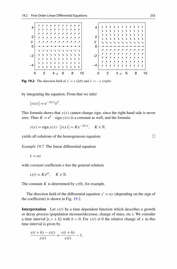
19.2 First-Order Linear Differential Equations 255
Fig. 19.2 The direction field of y′ = y (left) and y′ = −y (right)
by integrating the equation. From that we infer
∣∣y(x)∣∣ = e−A(x)eC.
This formula shows that y(x) cannot change sign, since the right-hand side is neverzero. Thus K = eC · signy(x) is a constant as well, and the formula
y(x) = signy(x) · ∣∣y(x)∣∣ = Ke−A(x), K ∈ R
yields all solutions of the homogeneous equation. �
Example 19.7 The linear differential equation
x = ax
with constant coefficient a has the general solution
x(t) = Keat , K ∈ R.
The constant K is determined by x(0), for example.
The direction field of the differential equation y′ = ay (depending on the sign ofthe coefficient) is shown in Fig. 19.2.
Interpretation Let x(t) be a time dependent function which describes a growthor decay process (population increase/decrease, change of mass, etc.). We considera time interval [t, t + h] with h > 0. For x(t) �= 0 the relative change of x in thistime interval is given by
x(t + h) − x(t)
x(t)= x(t + h)
x(t)− 1.

256 19 Differential Equations
Fig. 19.3 Radioactive decaywith constantsa = −0.5,−1,−2 (top tobottom)
The relative rate of change (change per unit of time) is thus
x(t + h) − x(t)
t + h − t· 1
x(t)= x(t + h) − x(t)
h · x(t).
For an ideal growth process this rate only depends on time t . In the limit h → 0 thisleads to the instantaneous relative rate of change
a(t) = limh→0
x(t + h) − x(t)
h · x(t)= x(t)
x(t).
Ideal growth processes thus may be modelled by the linear differential equation
x(t) = a(t)x(t).
Example 19.8 (Radioactive decay) Let x(t) be the concentration of a radioactivesubstance at time t . In radioactive decay the rate of change does not depend on timeand is negative,
a(t) ≡ a < 0.
The solution of the equation x = ax with initial value x(0) = x0 is
x(t) = eatx0.
It is exponentially decreasing and limt→∞ x(t) = 0; see Fig. 19.3. The half life T ,the time in which half of the substance has decayed, is obtained from
x0
2= eaT x0 as T = − log 2
a.
The half life for a = −2 is indicated in Fig. 19.3 by the dotted lines.
Example 19.9 (Population models) Let x(t) be the size of a population at time t ,modelled by x = ax. If a constant, positive rate of growth, a > 0, is presumed, thenthe population grows exponentially
x(t) = eatx0, limt→∞
∣∣x(t)∣∣ = ∞.
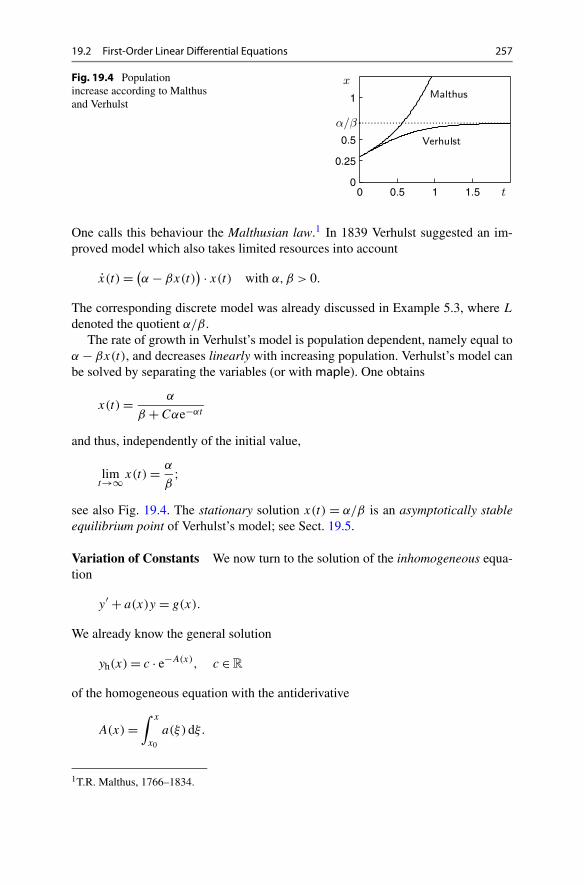
19.2 First-Order Linear Differential Equations 257
Fig. 19.4 Populationincrease according to Malthusand Verhulst
One calls this behaviour the Malthusian law.1 In 1839 Verhulst suggested an im-proved model which also takes limited resources into account
x(t) = (α − βx(t)
) · x(t) with α,β > 0.
The corresponding discrete model was already discussed in Example 5.3, where L
denoted the quotient α/β .The rate of growth in Verhulst’s model is population dependent, namely equal to
α − βx(t), and decreases linearly with increasing population. Verhulst’s model canbe solved by separating the variables (or with maple). One obtains
x(t) = α
β + Cαe−αt
and thus, independently of the initial value,
limt→∞x(t) = α
β;
see also Fig. 19.4. The stationary solution x(t) = α/β is an asymptotically stableequilibrium point of Verhulst’s model; see Sect. 19.5.
Variation of Constants We now turn to the solution of the inhomogeneous equa-tion
y′ + a(x)y = g(x).
We already know the general solution
yh(x) = c · e−A(x), c ∈ R
of the homogeneous equation with the antiderivative
A(x) =∫ x
x0
a(ξ)dξ.
1T.R. Malthus, 1766–1834.

258 19 Differential Equations
We look for a particular solution of the inhomogeneous equation of the form
yp(x) = c(x) · yh(x) = c(x) · e−A(x),
where we allow the constant c = c(x) to be a function of x (variation of constant).Substituting this formula into the inhomogeneous equation and differentiating usingthe product rule yields
y′p(x) + a(x)yp(x) = c′(x)yh(x) + c(x)y′
h(x) + a(x)yp(x)
= c′(x)yh(x) − a(x)c(x)yh(x) + a(x)yp(x)
= c′(x)yh(x).
If one equates this expression with the inhomogeneity g(x), one recognises that c(x)
fulfills the differential equation
c′(x) = eA(x)g(x),
which can be solved by integration,
c(x) =∫ x
x0
eA(ξ)g(ξ)dξ.
We thus obtain the following proposition.
Proposition 19.10 The differential equation
y′ + a(x)y = g(x)
has the general solution
y(x) = e−A(x)
(∫ x
x0
eA(ξ)g(ξ)dξ + K
)
with A(x) = ∫ x
x0a(ξ)dξ and an arbitrary constant K ∈ R.
Proof By the above considerations, the function y(x) is a solution of the differen-tial equation y′ + a(x)y = g(x). Conversely, let z(x) be any other solution. Then,according to the superposition principle, the difference z(x) − y(x) is a solution ofthe homogeneous equation, so
z(x) = y(x) + ce−A(x).
Therefore, z(x) also has the form stated in the proposition. �
Corollary 19.11 Let yp be an arbitrary solution of the inhomogeneous linear dif-ferential equation
y′ + a(x)y = g(x).

19.3 Existence and Uniqueness of the Solution 259
Then its general solution can be written as
y(x) = yp(x) + yh(x) = yp(x) + Ke−A(x), K ∈ R.
Proof This statement follows from the proof of Proposition 19.10 or directly fromthe superposition principle. �
Example 19.12 We solve the problem y′ + 2y = e4x + 1. The solution of the homo-geneous equation is yh(x) = ce−2x . A particular solution can be found by variationof constants. From
c(x) =∫ x
0e2ξ
(e4ξ + 1
)dξ = 1
6e6x + 1
2e2x − 2
3
it follows that
yp(x) = 1
6e4x − 2
3e−2x + 1
2.
The general solution is thus
y(x) = yp(x) + yh(x) = Ke−2x + 1
6e4x + 1
2.
Here, we have combined the two terms containing e−2x . The new constant K canbe determined from an additional initial condition y(0) = α, namely
K = α − 2
3.
19.3 Existence and Uniqueness of the Solution
Finding analytic solutions of differential equations can be a difficult problem andis often impossible. Apart from some types of differential equations (for example,linear problems or equations with separable variables), there is no general procedureto determine the solution explicitly. Thus numerical methods are used frequently(see Chap. 21). In the following we discuss the existence and uniqueness of solutionsof general initial value problems.
Proposition 19.13 (Peano’s theorem2) If the function f is continuous in a neigh-bourhood of (x0, y0), then the initial value problem
y′ = f (x, y), y(x0) = y0
has a solution y(x) for x close to x0.
2G. Peano, 1858–1932.

260 19 Differential Equations
Instead of a proof (see [11, Part I, Theorem 7.6]), we discuss the limitationsof this proposition. First it only guarantees the existence of a local solution in theneighbourhood of the initial value. The next example shows that one cannot expectmore, in general.
Example 19.14 We solve the differential equation x = x2, x(0) = 1. Separation ofthe variables yields
∫dx
x2=
∫dt = t + C,
and thus
x(t) = 1
1 − t.
This function has a singularity at t = 1, where the solution ceases to exist. Thisbehaviour is called blow up.
Furthermore, Peano’s theorem does not give any information on how many so-lutions an initial value problem has. In general, solutions need not be unique, as isshown in the following example.
Example 19.15 The initial value problem y′ = 2√|y|, y(0) = 0 has infinitely many
solutions
y(x) =
⎧⎪⎨⎪⎩
(x − b)2 b < x,
0 −a ≤ x ≤ b,
−(x − a)2 x < −a,
a, b ≥ 0 arbitrary.
For example, for x < −a, one verifies at once
y ′(x) = −2(x − a) = 2(a − x) = 2|x − a| = 2√
(x − a)2 = 2√|y|.
Thus the continuity of f is not sufficient to guarantee the uniqueness of the so-lution of initial value problems. One needs somewhat more regularity, namely Lip-schitz3 continuity with respect to the second variable (see also Definition 24.14).
Definition 19.16 Let D ⊂ R2 and f : D → R. The function f is said to satisfy
a Lipschitz condition with Lipschitz constant L on D, if the inequality |f (x, y) −f (x, z)| ≤ L|y − z| holds for all points (x, y), (x, z) ∈ D.
3R. Lipschitz, 1832–1903.
19.3 Existence and Uniqueness of the Solution 261
According to the mean value theorem (Proposition 8.4)
f (x, y) − f (x, z) = ∂f
∂y(x, ξ)(y − z)
for every differentiable function. If the derivative is bounded, then the function sat-isfies a Lipschitz condition. In this case one can choose
L = sup
∣∣∣∣∂f∂y (x, ξ)
∣∣∣∣.
Counterexample 19.17 The function g(x, y) = √|y| does not satisfy a Lipschitzcondition in any D that contains a point with y = 0 because
|g(x, y) − g(x,0)||y − 0| =
√|y||y| = 1√|y| → ∞ for y → 0.
Proposition 19.18 If the function f satisfies a Lipschitz condition in the neighbour-hood of (x0, y0), then the initial value problem
y′ = f (x, y), y(x0) = y0
has a unique solution y(x) for x close to x0.
Proof We only show uniqueness, the existence of a solution y(x) on the interval[x0, x0 + H ] follows (for small H ) from Peano’s theorem. Uniqueness is provenindirectly. Assume that z is another solution, different from y, on the interval[x0, x0 + H ] with z(x0) = y0. The number
x1 = inf{x ∈ R; x0 ≤ x ≤ x0 + H and y(x) �= z(x)
}
is thus well-defined. We infer from the continuity of y and z that y(x1) = z(x1).Now we choose h > 0 so small that x1 + h ≤ x0 + H and integrate the differentialequation
y′(x) = f(x, y(x)
)
from x1 to x1 + h. This gives
y(x1 + h) − y(x1) =∫ x1+h
x1
y′(x)dx =∫ x1+h
x1
f(x, y(x)
)dx
and
z(x1 + h) − y(x1) =∫ x1+h
x1
f(x, z(x)
)dx.
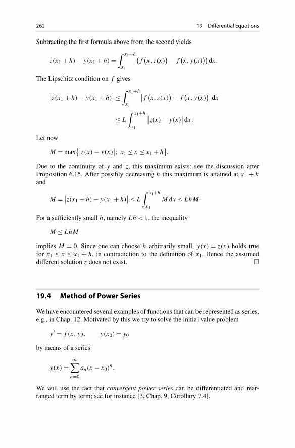
262 19 Differential Equations
Subtracting the first formula above from the second yields
z(x1 + h) − y(x1 + h) =∫ x1+h
x1
(f
(x, z(x)
) − f(x, y(x)
))dx.
The Lipschitz condition on f gives
∣∣z(x1 + h) − y(x1 + h)∣∣ ≤
∫ x1+h
x1
∣∣f (x, z(x)
) − f(x, y(x)
)∣∣dx
≤ L
∫ x1+h
x1
∣∣z(x) − y(x)∣∣dx.
Let now
M = max{∣∣z(x) − y(x)
∣∣; x1 ≤ x ≤ x1 + h}.
Due to the continuity of y and z, this maximum exists; see the discussion afterProposition 6.15. After possibly decreasing h this maximum is attained at x1 + h
and
M = ∣∣z(x1 + h) − y(x1 + h)∣∣ ≤ L
∫ x1+h
x1
M dx ≤ LhM.
For a sufficiently small h, namely Lh < 1, the inequality
M ≤ LhM
implies M = 0. Since one can choose h arbitrarily small, y(x) = z(x) holds truefor x1 ≤ x ≤ x1 + h, in contradiction to the definition of x1. Hence the assumeddifferent solution z does not exist. �
19.4 Method of Power Series
We have encountered several examples of functions that can be represented as series,e.g., in Chap. 12. Motivated by this we try to solve the initial value problem
y′ = f (x, y), y(x0) = y0
by means of a series
y(x) =∞∑
n=0
an(x − x0)n.
We will use the fact that convergent power series can be differentiated and rear-ranged term by term; see for instance [3, Chap. 9, Corollary 7.4].

19.4 Method of Power Series 263
Example 19.19 We solve once more the linear initial value problem
y′ = y, y(0) = 1.
In order to do so, we differentiate the ansatz
y(x) =∞∑
n=0
anxn = a0 + a1x + a2x
2 + a3x3 + · · ·
term by term with respect to x,
y′(x) =∞∑
n=1
nanxn−1 = a1 + 2a2x + 3a3x
2 + 4a4x3 + · · · ,
and substitute the result into the differential equation to get
a1 + 2a2x + 3a3x2 + 4a4x
3 + · · · = a0 + a1x + a2x2 + a3x
3 + · · · .
Since this equation has to hold for all x, the unknowns an can be determined byequating the coefficients of same powers of x. This gives
a1 = a0, 2a2 = a1,
3a3 = a2, 4a4 = a3,
and so on. Due to a0 = y(0) = 1 this infinite system of equations can be solvedrecursively. One obtains
a0 = 1, a1 = 1, a2 = 1
2! , a3 = 1
3! , . . . , an = 1
n!and thus the (expected) solution
y(x) =∞∑
n=0
xn
n! = ex.
Example 19.20 (A particular Riccati differential equation 4) For the solution of theinitial value problem
y′ = y2 + x2, y(0) = 1,
we make the ansatz
y(x) =∞∑
n=0
anxn = a0 + a1x + a2x
2 + a3x3 + · · · .
4J.F. Riccati, 1676–1754.
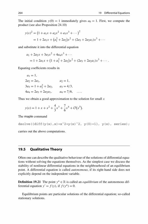
264 19 Differential Equations
The initial condition y(0) = 1 immediately gives a0 = 1. First, we compute theproduct (see also Proposition 24.10)
y(x)2 = (1 + a1x + a2x
2 + a3x3 + · · · )2
= 1 + 2a1x + (a2
1 + 2a2)x2 + (2a3 + 2a2a1)x
3 + · · ·and substitute it into the differential equation
a1 + 2a2x + 3a3x2 + 4a4x
3 + · · ·= 1 + 2a1x + (
1 + a21 + 2a2
)x2 + (2a3 + 2a2a1)x
3 + · · · .
Equating coefficients results in
a1 = 1,
2a2 = 2a1, a2 = 1,
3a3 = 1 + a21 + 2a2, a3 = 4/3,
4a4 = 2a3 + 2a2a1, a4 = 7/6, . . . .
Thus we obtain a good approximation to the solution for small x
y(x) = 1 + x + x2 + 4
3x3 + 7
6x4 + O
(x5).
The maple command
dsolve({diff(y(x),x)=xˆ2+y(x)ˆ2, y(0)=1}, y(x), series);
carries out the above computations.
19.5 Qualitative Theory
Often one can describe the qualitative behaviour of the solutions of differential equa-tions without solving the equations themselves. As the simplest case we discuss thestability of nonlinear differential equations in the neighbourhood of an equilibriumpoint. A differential equation is called autonomous, if its right-hand side does notexplicitly depend on the independent variable.
Definition 19.21 The point y� ∈ R is called an equilibrium of the autonomous dif-ferential equation y′ = f (y), if f (y�) = 0.
Equilibrium points are particular solutions of the differential equation; so-calledstationary solutions.

19.5 Qualitative Theory 265
In order to investigate solutions in the neighbourhood of an equilibrium point,we linearise the differential equation at the equilibrium. Let
w(x) = y(x) − y�
denote the distance of the solution y(x) from the equilibrium. Taylor series expan-sion of f shows that
w′ = y′ = f (y) = f (y) − f (y�) = f ′(y�)w + O(w2),
hence
w′(x) = (a + O(w)
)w
with a = f ′(y�). It is decisive how solutions of this problem behave for small w. Ob-viously the value of the coefficient a+ O(w) is crucial. If a < 0, then a + O(w) < 0for sufficiently small w and the function |w(x)| decreases. If on the other handa > 0, then the function |w(x)| increases for small w. With these considerationsone has proven the following proposition.
Proposition 19.22 Let y� be an equilibrium point of the differential equationy′ = f (y) and assume that f ′(y�) < 0. Then all solutions of the differential equa-tion with initial value w(0) close to y� satisfy the estimate
∣∣w(x)∣∣ ≤ C · ebx · ∣∣w(0)
∣∣with constants C > 0 and b < 0.
Under the conditions of the proposition one calls the equilibrium point asymp-totically stable. An asymptotically stable equilibrium attracts all solutions in a suf-ficiently small neighbourhood (exponentially fast), since due to b < 0
∣∣w(x)∣∣ → 0 as x → ∞.
Example 19.23 Verhulst’s model,
y′ = (α − βy)y, α,β > 0,
has two equilibrium points, namely y�1 = 0 and y�
2 = α/β . Due to
f ′(y�1) = α − 2βy�
1 = α, f ′(y�2) = α − 2βy�
2 = −α,
y�1 = 0 is unstable and y�
2 = α/β is asymptotically stable.

266 19 Differential Equations
19.6 Exercises
1. Find the general solution of the following differential equations and sketch somesolution curves
(a) x = x
t, (b) x = t
x, (c) x = −t
x.
The direction field is most easily plotted with maple, e.g., with DEplot.2. Using the applet Dynamical systems in the plane, solve Exercise 1 by rewrit-
ing the respective differential equation as an equivalent autonomous system byadding the equation t = 1.Hint. The variables are denoted by x and y in the applet. For example, Exer-cise 1(a) would have to be written as x′ = x/y and y′ = 1.
3. According to Newton’s law of cooling, the rate of change of the temperature x
of an object is proportional to the difference of its temperature and the ambienttemperature a. This is modelled by the differential equation
x = k(a − x),
where k is a proportionality constant. Find the general solution of this differentialequation.How long does it take to cool down an object from x(0) = 100° to 40° at anambient temperature of 20°, if it cooled down from 100° to 80° in 5 minutes?
4. Solve Verhulst’s differential equation from Example 19.9 and compute the limitt → ∞ of the solution.
5. A tank contains 100 l of liquid A. Liquid B is added at a rate of 5 l/s, while at thesame time the mixture is pumped out with a rate of 10 l/s. We are interested inthe amount x(t) of the liquid B in the tank at time t . From the balance equationx(t) = rate(in) − rate(out) = rate(in) − 10 · x(t)/total amount(t) one obtains thedifferential equation
x = 5 − 10x
100 − 5t, x(0) = 0.
Explain the derivation of this equation in detail and use maple (with dsolve)to solve the initial value problem. When is the tank empty?

20Systems of Differential Equations
Systems of differential equations, often called differentiable dynamical systems,play a vital role in modelling time dependent processes in mechanics, meteorol-ogy, biology, medicine, economics and other sciences. We limit ourselves to two-dimensional systems, whose solutions (trajectories) can be graphically representedas curves in the plane. The first section introduces linear systems, which can besolved analytically as will be shown. In many applications, however, nonlinear sys-tems are required. In general, their solution cannot be given explicitly. Here it isof primary interest to understand the qualitative behaviour of solutions. In the sec-ond section of this chapter, we touch upon the rich qualitative theory of dynamicalsystems. Numerical methods will be discussed in Chap. 21.
20.1 Systems of Linear Differential Equations
We start with the description of various situations which lead to systems of differ-ential equations. In Chap. 19 Malthus’ population model was presented, where therate of change of a population x(t) was assumed to be proportional to the existingpopulation:
x(t) = ax(t).
The presence of a second population y(t) could result in a decrease or increase ofthe rate of change of x(t). Conversely, the population x(t) could also affect the rateof change of y(t). This results in a coupled system of equations,
x(t) = ax(t) + by(t),
y(t) = cx(t) + dy(t),
with positive or negative coefficients b and c, which describe the interaction of thepopulations. This is the general form of a linear system of differential equations in
M. Oberguggenberger, A. Ostermann, Analysis for Computer Scientists,Undergraduate Topics in Computer Science,DOI 10.1007/978-0-85729-446-3_20, © Springer-Verlag London Limited 2011
267

268 20 Systems of Differential Equations
two unknowns, written briefly as
x = ax + by,
y = cx + dy.
Refined models are obtained if one takes into account the dependence of the rate ofgrowth on food supply, for instance. For one species this would result in an equationof the form
x = (v − n)x,
where v denotes the available food supply and n a threshold value. So, the popula-tion is increasing if the available quantity of food is larger than n, and is otherwisedecreasing. In the case of a predator–prey relationship of species x to species y,in which y is the food for x, the relative rates of change are not constant. A com-mon assumption is that these rates contain a term that depends linearly on the otherspecies. Under this assumption, one obtains the nonlinear system
x = (ay − n)x,
y = (d − cx)y.
This is the famous predator–prey model of Lotka1 and Volterra2 (for a detailedderivation we refer to [13, Chap. 12.2]).
The general form of a system of nonlinear differential equations is
x = f (x, y),
y = g(x, y).
Geometrically this can be interpreted in the following way. The right-hand side de-fines a vector field
(x, y) �→[f (x, y)g(x, y)
]
on R2; the left-hand side is the velocity vector of a plane curve
t �→[x(t)y(t)
].
The solutions are thus plane curves whose velocity vectors are given by the vectorfield.
Example 20.1 (Rotation of the plane) The vector field
(x, y) �→[−y
x
]
1A.J. Lotka, 1880–1949.2V. Volterra, 1860–1940.
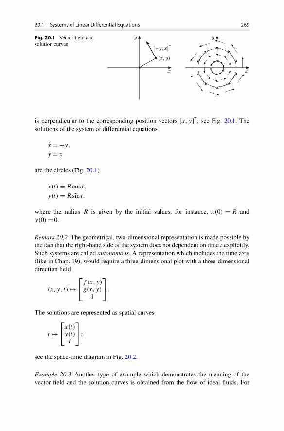
20.1 Systems of Linear Differential Equations 269
Fig. 20.1 Vector field andsolution curves
is perpendicular to the corresponding position vectors [x, y]T; see Fig. 20.1. Thesolutions of the system of differential equations
x = −y,
y = x
are the circles (Fig. 20.1)
x(t) = R cos t,
y(t) = R sin t,
where the radius R is given by the initial values, for instance, x(0) = R andy(0) = 0.
Remark 20.2 The geometrical, two-dimensional representation is made possible bythe fact that the right-hand side of the system does not dependent on time t explicitly.Such systems are called autonomous. A representation which includes the time axis(like in Chap. 19), would require a three-dimensional plot with a three-dimensionaldirection field
(x, y, t) �→⎡⎣f (x, y)
g(x, y)1
⎤⎦ .
The solutions are represented as spatial curves
t �→⎡⎣x(t)
y(t)t
⎤⎦ ;
see the space-time diagram in Fig. 20.2.
Example 20.3 Another type of example which demonstrates the meaning of thevector field and the solution curves is obtained from the flow of ideal fluids. For

270 20 Systems of Differential Equations
Fig. 20.2 Direction field andspace–time diagram forx = −y, y = x
example,
x = 1 − x2 − y2
(x2 + y2)2,
y = −2xy
(x2 + y2)2
describes a plane, stationary potential flow around the cylinder x2 + y2 ≤ 1(Fig. 20.3). The right-hand side describes the flow velocity at the point (x, y). Thesolution curves follow the stream lines
y
(1 − 1
x2 + y2
)= C.
Here C denotes a constant. This can be checked by differentiating the above relationwith respect to t and substituting x and y by the right-hand side of the differentialequation.
Experiment 20.4 Using the applet Dynamical systems in the plane, study the vec-tor field and the solution curves of the system of differential equations from Exam-ples 20.1 and 20.3. In a similar way, study the systems of differential equations
x = y, x = y, x = −y, x = x, x = y,
y = −x, y = x, y = −x, y = x, y = y,
and try to understand the behaviour of the solution curves.
Before turning to the solution theory of planar linear systems of differential equa-tions, it is useful to introduce a couple of notions that serve to describe the qualitativebehaviour of solution curves. The system of differential equations
x(t) = f(x(t), y(t)
),
y(t) = g(x(t), y(t)
)

20.1 Systems of Linear Differential Equations 271
Fig. 20.3 Plane potentialflow around a cylinder
together with prescribed values at t = 0
x(0) = x0, y(0) = y0,
is again called an initial value problem. In this chapter we assume the functionsf and g to be at least continuous. By a solution curve or a trajectory we meana continuously differentiable curve t �→ [x(t) y(t)]T whose components fulfill thesystem of differential equations.
For the case of a single differential equation the notion of an equilibrium pointwas introduced in Definition 19.21. For systems of differential equations one has ananalogous notion.
Definition 20.5 (Equilibrium point) A point (x∗, y∗) is called equilibrium pointor equilibrium of the system of differential equations, if f (x∗, y∗) = 0 andg(x∗, y∗) = 0.
The name comes from the fact that a solution with initial value x0 = x∗, y0 = y∗remains at (x∗, y∗) for all times; in other words, if (x∗, y∗) is an equilibrium point,then x(t) = x∗, y(t) = y∗ is a solution to the system of differential equations, sinceboth the left- and right-hand side will be zero.
From Chap. 19 we know that solutions of differential equations do not have toexist for large times. However, if solutions with initial values in a neighbourhood ofan equilibrium point exist for all times, then the following notions are meaningful.
Definition 20.6 Let (x∗, y∗) be an equilibrium point. If there is a neighbourhoodU of (x∗, y∗) so that all trajectories with initial values (x0, y0) in U converge to theequilibrium point (x∗, y∗) as t → ∞, then this equilibrium is called asymptoticallystable. If for every neighbourhood V of (x∗, y∗) there is a neighbourhood W of(x∗, y∗) so that all trajectories with initial values (x0, y0) in W stay entirely in V ,then the equilibrium (x∗, y∗) is called stable. An equilibrium point which is notstable is called unstable.

272 20 Systems of Differential Equations
In short, stability means that trajectories that start close to the equilibrium pointremain close to it; asymptotic stability means that the trajectories are attracted bythe equilibrium point. In the case of an unstable equilibrium point there are trajec-tories that move away from it; in linear systems these trajectories are unbounded, inthe nonlinear case they can also converge to another equilibrium or a periodic so-lution (for instance, see the discussion of the mathematical pendulum in Sect. 20.2or [13]).
In the following we determine the solution to the initial value problem
x = ax + by, x(0) = x0,
y = cx + dy, y(0) = y0.
This is a two-dimensional system of first-order linear differential equations. For thispurpose we first discuss the three basic types of such systems and then show howarbitrary systems can be transformed to a system of basic type.
We denote the coefficient matrix by
A =[a b
c d
].
The decisive question is whether A is similar to a matrix of type I, II or III, asdescribed in Sect. 23.2. A matrix of type I has real eigenvalues and is similar to adiagonal matrix. A matrix of type II has a double real eigenvalue, its canonical form,however, contains a nilpotent part. The case of two complex conjugate eigenvaluesis finally covered by type III.
Type I—Real Eigenvalues, Diagonalisable Matrix In this case the standard formof the system is
x = αx, x(0) = x0,
y = βy, y(0) = y0.
We know from Example 19.7 that the solutions are given by
x(t) = x0eαt , y(t) = y0eβt
and in particular exist for all times t ∈ R. Obviously (x∗, y∗) = (0,0) is an equilib-rium point. If α < 0 and β < 0, then all solution curves approach the equilibrium(0,0) as t → ∞; this equilibrium is asymptotically stable. If α ≥ 0, β ≥ 0 (not bothequal to zero), then the solution curves leave every neighbourhood of (0,0) and theequilibrium is unstable. Similarly, instability is present in the case where α > 0,β < 0 (or vice versa). One calls such an equilibrium a saddle point.
If α = 0 and x0 = 0, then one can solve for t and represent the solution curves asgraphs of functions:
et =(
x
x0
)1/α
, y = y0
(x
x0
)β/α
.
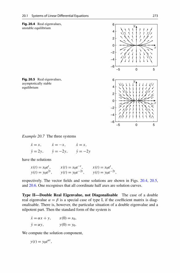
20.1 Systems of Linear Differential Equations 273
Fig. 20.4 Real eigenvalues,unstable equilibrium
Fig. 20.5 Real eigenvalues,asymptotically stableequilibrium
Example 20.7 The three systems
x = x, x = −x, x = x,
y = 2y, y = −2y, y = −2y
have the solutions
x(t) = x0et , x(t) = x0e−t , x(t) = x0et ,
y(t) = y0e2t , y(t) = y0e−2t , y(t) = y0e−2t ,
respectively. The vector fields and some solutions are shown in Figs. 20.4, 20.5,and 20.6. One recognises that all coordinate half axes are solution curves.
Type II—Double Real Eigenvalue, not Diagonalisable The case of a doublereal eigenvalue α = β is a special case of type I, if the coefficient matrix is diag-onalisable. There is, however, the particular situation of a double eigenvalue and anilpotent part. Then the standard form of the system is
x = αx + y, x(0) = x0,
y = αy, y(0) = y0.
We compute the solution component,
y(t) = y0eαt ,

274 20 Systems of Differential Equations
Fig. 20.6 Real eigenvalues,saddle point
Fig. 20.7 Double realeigenvalue, matrix notdiagonalisable
substitute it into the first equation,
x(t) = αx(t) + y0eαt , x(0) = x0,
and apply the variation of constants formula from Chap. 19:
x(t) = eαt
(x0 +
∫ t
0e−αsy0eαs ds
)= eαt (x0 + ty0).
The vector fields and some solution curves for the case α = −1 are depicted inFig. 20.7.
Type III—Complex Conjugate Eigenvalues In this case the standard form of thesystem is
x = αx − βy, x(0) = x0,
y = βx + αy, y(0) = y0.
By introducing the complex variable z and the complex coefficients γ, z0 as
z = x + iy, γ = α + iβ, z0 = x0 + iy0,
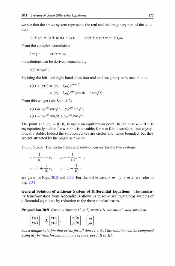
20.1 Systems of Linear Differential Equations 275
we see that the above system represents the real and the imaginary part of the equa-tion
(x + iy) = (α + iβ)(x + iy), x(0) + iy(0) = x0 + iy0.
From the complex formulation
z = γ z, z(0) = z0,
the solutions can be derived immediately:
z(t) = z0eγ t .
Splitting the left- and right-hand sides into real and imaginary part, one obtains
x(t) + iy(t) = (x0 + iy0)e(α+iβ)t
= (x0 + iy0)eαt (cosβt + i sinβt).
From this we get (see Sect. 4.2)
x(t) = x0eαt cosβt − y0eαt sinβt,
y(t) = x0eαt sinβt + y0eαt cosβt.
The point (x∗, y∗) = (0,0) is again an equilibrium point. In the case α < 0 it isasymptotically stable; for α > 0 it is unstable; for α = 0 it is stable but not asymp-totically stable. Indeed the solution curves are circles and hence bounded, but theyare not attracted by the origin as t → ∞.
Example 20.8 The vector fields and solution curves for the two systems
x = 1
10x − y, x = − 1
10x − y,
y = x + 1
10y, y = x − 1
10y
are given in Figs. 20.8 and 20.9. For the stable case, x = −y, y = x, we refer toFig. 20.1.
General Solution of a Linear System of Differential Equations The similar-ity transformation from Appendix B allows us to solve arbitrary linear systems ofdifferential equations by reduction to the three standard cases.
Proposition 20.9 For an arbitrary (2 × 2)-matrix A, the initial value problem[x(t)
y(t)
]= A
[x(t)
y(t)
],
[x(0)
y(0)
]=
[x0y0
]
has a unique solution that exists for all times t ∈ R. This solution can be computedexplicitly by transformation to one of the types I, II or III.
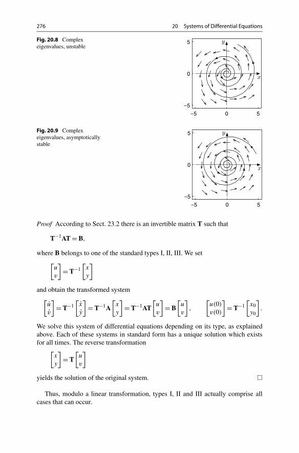
276 20 Systems of Differential Equations
Fig. 20.8 Complexeigenvalues, unstable
Fig. 20.9 Complexeigenvalues, asymptoticallystable
Proof According to Sect. 23.2 there is an invertible matrix T such that
T−1AT = B,
where B belongs to one of the standard types I, II, III. We set[u
v
]= T−1
[x
y
]
and obtain the transformed system[u
v
]= T−1
[x
y
]= T−1A
[x
y
]= T−1AT
[u
v
]= B
[u
v
],
[u(0)
v(0)
]= T−1
[x0y0
].
We solve this system of differential equations depending on its type, as explainedabove. Each of these systems in standard form has a unique solution which existsfor all times. The reverse transformation[
x
y
]= T
[u
v
]
yields the solution of the original system. �
Thus, modulo a linear transformation, types I, II and III actually comprise allcases that can occur.
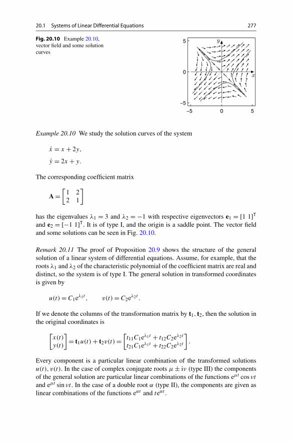
20.1 Systems of Linear Differential Equations 277
Fig. 20.10 Example 20.10,vector field and some solutioncurves
Example 20.10 We study the solution curves of the system
x = x + 2y,
y = 2x + y.
The corresponding coefficient matrix
A =[
1 22 1
]
has the eigenvalues λ1 = 3 and λ2 = −1 with respective eigenvectors e1 = [1 1]T
and e2 = [−1 1]T. It is of type I, and the origin is a saddle point. The vector fieldand some solutions can be seen in Fig. 20.10.
Remark 20.11 The proof of Proposition 20.9 shows the structure of the generalsolution of a linear system of differential equations. Assume, for example, that theroots λ1 and λ2 of the characteristic polynomial of the coefficient matrix are real anddistinct, so the system is of type I. The general solution in transformed coordinatesis given by
u(t) = C1eλ1t , v(t) = C2eλ2t .
If we denote the columns of the transformation matrix by t1, t2, then the solution inthe original coordinates is
[x(t)
y(t)
]= t1u(t) + t2v(t) =
[t11C1eλ1t + t12C2eλ2t
t21C1eλ1t + t22C2eλ2t
].
Every component is a particular linear combination of the transformed solutionsu(t), v(t). In the case of complex conjugate roots μ ± iν (type III) the componentsof the general solution are particular linear combinations of the functions eμt cosνt
and eμt sinνt . In the case of a double root α (type II), the components are given aslinear combinations of the functions eαt and teαt .

278 20 Systems of Differential Equations
20.2 Systems of Nonlinear Differential Equations
In contrast to linear systems of differential equations, the solutions to nonlinearsystems can generally not be expressed by explicit formulae. Apart from numericalmethods (Chap. 21) the qualitative theory is of interest. It describes the behaviour ofsolutions without knowing them explicitly. In this section we will demonstrate thiswith the help of two examples.
The Lotka–Volterra Model In Sect. 20.1 the predator–prey model of Lotka andVolterra was introduced. In order to simplify the presentation, we set all coefficientsequal to one. Thus the system becomes
x = x(y − 1),
y = y(1 − x).
The equilibrium points are (x∗, y∗) = (1,1) and (x∗∗, y∗∗) = (0,0). Obviously, thecoordinate half axes are solution curves given by
x(t) = x0e−t , x(t) = 0,
y(t) = 0, y(t) = y0et .
The equilibrium (0,0) is thus a saddle point (unstable); we will later analyse thetype of equilibrium (1,1). In the following we will only consider the first quadrantx ≥ 0, y ≥ 0, which is relevant in biological models. Along the straight line x = 1the vector field is horizontal, along the straight line y = 1 it is vertical. It looks as ifthe solution curves rotate about the equilibrium point (1,1); see Fig. 20.11.
In order to be able to verify this conjecture we search for a function H(x,y)
which is constant along the solution curves:
H(x(t), y(t)
) = C.
Such a function is called a first integral, invariant or conserved quantity of the sys-tem of differential equations. Consequently, we have
d
dtH
(x(t), y(t)
) = 0
or by the chain rule for functions in two variables (Proposition 15.16)
∂H
∂xx + ∂H
∂yy = 0.
With the ansatz
H(x,y) = F(x) + G(y),
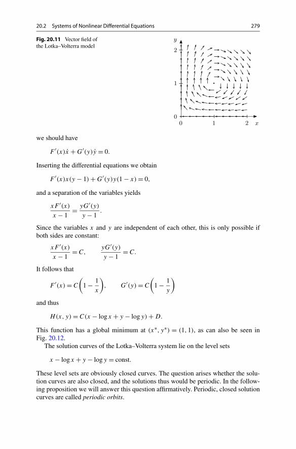
20.2 Systems of Nonlinear Differential Equations 279
Fig. 20.11 Vector field ofthe Lotka–Volterra model
we should have
F ′(x)x + G′(y)y = 0.
Inserting the differential equations we obtain
F ′(x)x(y − 1) + G′(y)y(1 − x) = 0,
and a separation of the variables yields
xF ′(x)
x − 1= yG′(y)
y − 1.
Since the variables x and y are independent of each other, this is only possible ifboth sides are constant:
xF ′(x)
x − 1= C,
yG′(y)
y − 1= C.
It follows that
F ′(x) = C
(1 − 1
x
), G′(y) = C
(1 − 1
y
)
and thus
H(x,y) = C(x − logx + y − logy) + D.
This function has a global minimum at (x∗, y∗) = (1,1), as can also be seen inFig. 20.12.
The solution curves of the Lotka–Volterra system lie on the level sets
x − logx + y − logy = const.
These level sets are obviously closed curves. The question arises whether the solu-tion curves are also closed, and the solutions thus would be periodic. In the follow-ing proposition we will answer this question affirmatively. Periodic, closed solutioncurves are called periodic orbits.
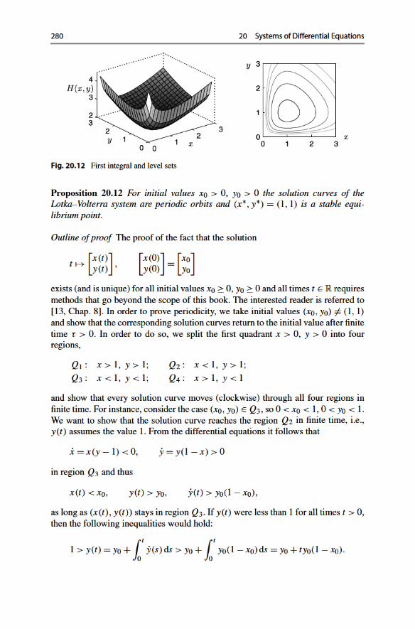

20.2 Systems of Nonlinear Differential Equations 281
Fig. 20.13 Solution curvesof the Lotka–Volterra model
However, the latter expression diverges to infinity as t → ∞, a contradiction. Con-sequently, y(t) has to reach the value 1 and thus the region Q2 in finite time. Like-wise one reasons for the other regions. Thus, there exists a time τ > 0 such that(x(τ ), y(τ )) = (x0, y0).
From this the periodicity of the orbit follows. Since the system of differentialequations is autonomous, t �→ (x(t + τ), y(t + τ)) is a solution as well. As justshown, both solutions have the same initial value at t = 0. The uniqueness of thesolution of initial value problems implies that the two solutions are identical, so
x(t) = x(t + τ), y(t) = y(t + τ)
is fulfilled for all times t ∈ R. However, this proves that the solution t �→ (x(t), y(t))
is periodic with period τ .All solution curves in the first quadrant with the exception of the equilibrium are
thus periodic orbits. Solution curves that start close to (x∗, y∗) = (1,1), stay close;see Fig. 20.12. The point (1,1) is thus a stable equilibrium. �
Figure 20.13 shows some solution curves. The populations of predator and preythus increase and decrease periodically and in opposite direction. For further popu-lation models we refer to [6].
Pendulum As a second example we consider the mathematical pendulum. It mod-els an object of mass m that is attached to the origin with a (massless) cord of lengthl and moves under the gravitational force −mg; see Fig. 20.14. The variable x(t)
denotes the angle of deflexion from the vertical direction, measured in counterclock-wise direction. The tangential acceleration of the object is equal to lx(t), the tan-gential component of the gravitational force is −mg sinx(t). According to Newton’slaw, force = mass × acceleration, we have
−mg sinx = mlx
or
x = −g
lsinx.

282 20 Systems of Differential Equations
Fig. 20.14 Derivation of thependulum equation
If we introduce the new variable y = x and, for simplicity, set the coefficient to 1,then we obtain the system
x = y, x(0) = x0,
y = − sinx, y(0) = y0
describing the mathematical pendulum. Here x denotes the angle of deflexion and y
the angular velocity of the object.Note that the linearisation
sinx = x + O(x3) ≈ x
for small angles x leads to the approximation
x = y,
y = −x.
Apart from the change in sign this system of differential equations coincides withthat of Example 20.1.
In order to describe the shape of the solutions for the mathematical pendulum,we search again for a first integral of the form
H(x,y) = F(x) + G(y).
As for the Lotka–Volterra model it follows that
F ′(x)y − G′(y) sinx = 0,F ′(x)
sinx= G′(y)
y= C,
and thus
F ′(x) = C sinx, G′(y) = Cy,
so
F(x) = −C cosx + D, G(y) = Cy2
2+ E.

20.3 Exercises 283
Fig. 20.15 Solution curves,mathematical pendulum
A suitable choice of constants (C = 1,D = 1,E = 0) yields
H(x,y) = y2
2+ 1 − cosx,
which corresponds just to the total energy of the pendulum. The solution curves forprescribed initial values (x0, y0) lie on the level sets H(x,y) = C, i.e.,
y2
2+ 1 − cosx = y2
0
2+ 1 − cosx0,
y = ±√
y20 − 2 cosx0 + 2 cosx.
Figure 20.15 shows some solution curves. There are unstable equilibria at y = 0,x = . . . ,−3π,−π,π,3π, . . . which are connected by limit curves. One of the twolimit curves passes through x0 = 0, y0 = 2. The solution with these initial values lieson the limit curve and approaches the equilibrium (π,0) as t → ∞, and (−π,0) ast → −∞. Initial values that lie between these limit curves (for instance the valuesx0 = 0, |y0| < 2) give rise to periodic solutions of small amplitude (less than π ). Thesolutions outside represent large oscillations where the pendulum loops. We remarkthat the effects of friction are not taken into account in this model.
20.3 Exercises
1. The space-time diagram of a two-dimensional system of differential equations(Remark 20.2) can be obtained by introducing time as third variable z(t) = t andpassing to the three-dimensional system
⎡⎢⎣
x
y
z
⎤⎥⎦ =
⎡⎢⎣
f (x, y)
g(x, y)
1
⎤⎥⎦ .
284 20 Systems of Differential Equations
Use this observation to visualise the systems from Examples 20.1 and 20.3. Studythe time depending solution curves with the applet Dynamical systems in space.
2. Compute the general solutions of the following three systems of differentialequations by transformation to standard form:
x = 3
5x − 4
5y, x = −3y, x = 7
4x − 5
4y,
y = −4
5x − 3
5y, y = x, y = 5
4x + 1
4y.
Visualise the solution curves with the applet Dynamical systems in the plane.3. Small, undamped oscillations of an object of mass m attached to a spring are
described by the differential equation
mx + kx = 0.
Here, x = x(t) denotes the displacement from the position of rest and k is thespring stiffness. Introduce the variable y = x and rewrite the second-order dif-ferential equation as a linear system of differential equations. Find the generalsolution.
4. A company deposits its profits in an account with continuous interest rate a%.The balance is denoted by x(t). Simultaneously the amount y(t) is withdrawncontinuously from the account, where the rate of withdrawal is equal to b% ofthe account balance. With r = a/100, s = b/100 this leads to the linear systemof differential equations
x(t) = r(x(t) − y(t)
),
y(t) = sx(t).
Find the solution (x(t), y(t)) for the initial values x(0) = 1, y(0) = 0 and analysehow big s can be in comparison to r so that the account balance x(t) is increasingfor all times without oscillations.
5. A national economy has two sectors (for instance industry and agriculture) withthe production volumes x1(t), x2(t) at time t . If one assumes that the invest-ments are proportional to the respective growth rate, then the classical model ofLeontief 3 [23, Chap. 9.5] states
x1(t) = a11x1(t) + a12x2(t) + b1x1(t) + c1(t),
x2(t) = a21x1(t) + a22x2(t) + b2x2(t) + c2(t).
Here aij denotes the required amount of goods from sector i to produce oneunit of goods in sector j . Further bi xi(t) are the investments, and ci(t) is theconsumption in sector i. Under the simplifying assumptions a11 = a22 = 0,
3W. Leontief, 1906–1999.

20.3 Exercises 285
a12 = a21 = a (0 < a < 1), b1 = b2 = 1, c1(t) = c2(t) = 0 (no consumption)one obtains the system of differential equations
x1(t) = x1(t) − ax2(t),
x2(t) = −ax1(t) + x2(t).
Find the general solution and discuss the result.6. Use the applet Dynamical systems in the plane to analyse the solution curves of
the differential equations of the mathematical pendulum and translate the math-ematical results to statements about the mechanical behaviour.

21Numerical Solution of Differential Equations
As we have seen in the previous two chapters, only particular classes of differentialequations can be solved analytically. Especially for nonlinear problems one has torely on numerical methods.
In this chapter we discuss several variants of Euler’s method, taking the latter asa prototype. Motivated by the Taylor expansion of the analytical solution we deduceEuler approximations and study their stability properties. In this way we introducethe reader to several important aspects of the numerical solution of differential equa-tions. We point out, however, that for most real-life applications one has to use moresophisticated numerical methods.
21.1 The Explicit Euler Method
The differential equation
y′(x) = f(x, y(x)
)
defines the slope of the tangent to the solution curve y(x). Expanding the solutionat the point x + h into a Taylor series,
y(x + h) = y(x) + hy′(x) + O(h2),
and inserting the above value for y′(x), one obtains
y(x + h) = y(x) + hf(x, y(x)
) + O(h2),
and consequently for small h we have the approximation
y(x + h) ≈ y(x) + hf(x, y(x)
).
This observation motivates the (explicit) Euler method.
M. Oberguggenberger, A. Ostermann, Analysis for Computer Scientists,Undergraduate Topics in Computer Science,DOI 10.1007/978-0-85729-446-3_21, © Springer-Verlag London Limited 2011
287

288 21 Numerical Solution of Differential Equations
Fig. 21.1 Equidistant grid points xj = x0 + jh
Fig. 21.2 Eulerapproximation toy′ = y, y(0) = 1
Euler’s Method For the numerical solution of the initial value problem
y′(x) = f(x, y(x)
), y(a) = y0
on the interval [a, b] we first divide the interval into N parts of length h = (b−a)/N
and define the grid points xj = x0 + jh, 0 ≤ j ≤ N ; see Fig. 21.1.The distance h between two grid points is called the step size. We look for a
numerical approximation yn to the exact solution y(xn) at xn, i.e. yn ≈ y(xn). Ac-cording to the considerations above we should have
y(xn+1) ≈ y(xn) + hf(xn, y(xn)
).
If one replaces the exact solution by the numerical approximation and ≈ by =,then one obtains the explicit Euler method
yn+1 = yn + hf (xn, yn),
which defines the approximation yn+1 as a function of yn.Starting from the initial value y0 one computes from this recursion the approx-
imations y1, y2, . . . , yN ≈ y(b). The points (xi, yi) are the vertices of a polygonwhich approximates the graph of the exact solution y(x). Figure 21.2 shows the ex-act solution of the differential equation y′ = y, y(0) = 1 as well as polygons definedby Euler’s method for three different step sizes.
Euler’s method is convergent of order 1; see [11, Chap. II.3]. On bounded inter-vals [a, b] one thus has the uniform error estimate
∣∣y(xn) − yn
∣∣ ≤ Ch

21.1 The Explicit Euler Method 289
for all n ≥ 1 and sufficiently small h with 0 ≤ nh ≤ b − a. The constant C dependson the length of the interval and the solution y(x); however, it does not depend onn and h.
Example 21.1 The solution of the initial value problem y′ = y, y(0) = 1 isy(x) = ex . For nh = 1 the numerical solution yn approximates the exact solutionat x = 1. Due to
yn = yn−1 + hyn−1 = (1 + h)yn−1 = · · · = (1 + h)ny0
we have
yn = (1 + h)n =(
1 + 1
n
)n
≈ e.
The convergence of Euler’s method thus implies
e = limn→∞
(1 + 1
n
)n
.
This formula for e was already deduced in Example 7.11.
In commercial software packages, methods of higher order are used for thenumerical integration, for example Runge–Kutta or multi-step methods. All thesemethods are refinements of Euler’s method. In modern implementations of these al-gorithms the error is automatically estimated and the step size adaptively adjustedto the problem. For more details, we refer to [11, 12].
Experiment 21.2 In MATLAB you can find information on the numerical solutionof differential equations by calling help funfun. For example, one can solve theinitial value problem
y′ = y2, y(0) = 0.9
on the interval [0,1] with the command
[x,y] = ode23(’qfun’,[0,1],0.9).
The file qfun.m has to contain the definition of the function
function yp = f(x,y)
yp = y.ˆ2 .
For a plot of the solution, one sets the option
myopt = odeset(’OutputFcn’,’odeplot’)

290 21 Numerical Solution of Differential Equations
and calls the solver by
[x,y] = ode23(’qfun’, [0,1], 0.9, myopt) .
Start the program with different initial values and observe the blow up for y(0) ≥ 1.
21.2 Stability and Stiff Problems
The linear differential equation
y′ = ay, y(0) = 1
has the solution
y(x) = eax.
For a ≤ 0 this solution has the following qualitative property, independent of thesize of a:
∣∣y(x)∣∣ ≤ 1 for all x ≥ 0.
We are investigating whether numerical methods preserve this property. In order todo so, we solve the differential equation with the explicit Euler method and obtain
yn = yn−1 + hayn−1 = (1 + ha)yn−1 = · · · = (1 + ha)ny0 = (1 + ha)n.
For −2 ≤ ha ≤ 0 the numerical solution obeys the same bound,
|yn| =∣∣(1 + ha)n
∣∣ = ∣∣1 + ha∣∣n ≤ 1,
as the exact solution. However, for ha < −2 a dramatic instability occurs althoughthe exact solution is harmless. In fact, all explicit methods have the same difficultiesin this situation: the solution is only stable under very restrictive conditions on thestep size. For the explicit Euler method the condition for stability is
−2 ≤ ha ≤ 0.
For a � 0 this implies a drastic restriction on the step size, which eventually makesthe method in this situation inefficient.
In this case a remedy is offered by implicit methods, for example, the implicitEuler method
yn+1 = yn + hf (xn+1, yn+1).
It differs from the explicit method by the fact that the slope of the tangent is nowtaken at the endpoint. For the determination of the numerical solution, a nonlinearequation has to be solved in general. Therefore, such methods are called implicit.The implicit Euler method has the same accuracy as the explicit one, but by far better

21.2 Stability and Stiff Problems 291
stability properties, as the following analysis shows. If one applies the implicit Eulermethod to the initial value problem
y′ = ay, y(0) = 1, with a ≤ 0,
one obtains
yn = yn−1 + hf (xn, yn) = yn−1 + hayn,
and therefore
yn = 1
1 − hayn−1 = · · · = 1
(1 − ha)ny0 = 1
(1 − ha)n.
The procedure is thus stable, i.e. |yn| ≤ 1, if∣∣(1 − ha)n∣∣ ≥ 1.
However, for a ≤ 0 this is fulfilled for all h ≥ 0. Thus the procedure is stable forarbitrarily large step sizes.
Remark 21.3 A differential equation is called stiff, if for its solution the implicitEuler method is more efficient than the explicit method. (Often it is dramaticallymore efficient.)
Example 21.4 (From [12, Chap. IV.1]) We integrate the initial value problem
y′ = −50(y − cosx), y(0) = 0.997.
Its exact solution is
y(x) = 2500
2501cosx + 50
2501sinx − 6503
250100e−50x
≈ cos(x − 0.02) − 0.0026e−50x.
The solution looks quite harmless and resembles cosx, but the equation is stiff witha = −50. Warned by the analysis above we expect difficulties for explicit methods.
We integrate this differential equation numerically on the interval [0,10] withthe explicit Euler method and step sizes h = 10/n with n = 250, 248 and 246.For n < 250, i.e. h > 1/25, exponential instabilities occur; see Fig. 21.3. This isconsistent with the considerations above, because the product ah satisfies ah ≤ −2for h > 1/25.
However, if one integrates the differential equation with the implicit Eulermethod, then even for very large step sizes no instabilities arise; see Fig. 21.4. Theimplicit Euler method is more costly than the explicit one, as the computation ofyn+1 from
yn+1 = yn + hf (xn+1, yn+1)
generally requires the solution of a nonlinear equation.

292 21 Numerical Solution of Differential Equations
Fig. 21.3 Instability of the explicit Euler method. In each case the pictures show the exact solutionand the approximating polygons of Euler’s method with n steps
Fig. 21.4 Stability of the implicit Euler method. In each case the pictures show the exact solutionand the approximating polygons of Euler’s method with n steps
21.3 Systems of Differential Equations
For the derivation of a simple numerical method for solving systems of differentialequations
x(t) = f(t, x(t), y(t)
), x(t0) = x0,
y(t) = g(t, x(t), y(t)
), y(t0) = y0,
one again starts from the Taylor expansion of the analytic solution
x(t + h) = x(t) + hx(t) + O(h2),
y(t + h) = y(t) + hy(t) + O(h2),
and replaces the derivatives by the right-hand sides of the differential equations. Forsmall step sizes h, this motivates the explicit Euler method
xn+1 = xn + hf (tn, xn, yn),
yn+1 = yn + hg(tn, xn, yn).
One interprets xn and yn as numerical approximations to the exact solution x(tn)
and y(tn) at time tn = t0 + nh.

21.4 Exercises 293
Fig. 21.5 Numerical computation of a periodic orbit of the Lotka–Volterra model. The systemwas integrated on the interval 0 ≤ t ≤ 14 with Euler’s method and constant step sizes h = 14/n forn = 250, 500 and 1000
Example 21.5 In Sect. 20.2 we have investigated the Lotka–Volterra model
x = x(y − 1),
y = y(1 − x).
In order to compute the periodic orbit through the point (x0, y0) = (2,2) numeri-cally, we apply the explicit Euler method and obtain the recursion
xn+1 = xn + hxn(yn − 1),
yn+1 = yn + hyn(1 − xn).
Starting from the initial values x0 = 2 and y0 = 2 this recursion determines thenumerical solution for n ≥ 0. The results for three different step sizes are depictedin Fig. 21.5. Note the linear convergence of the numerical solution for h → 0.
This numerical experiment shows that one has to choose a very small step sizein order to obtain the periodicity of the true orbit in the numerical solution. Alterna-tively, one can use numerical methods of higher order or—in the present example—also the following modification of Euler’s method:
xn+1 = xn + hxn(yn − 1),
yn+1 = yn + hyn(1 − xn+1).
In this method one uses instead of xn the updated value xn+1 for the computationof yn+1. The numerical results, obtained with this modified Euler method, are givenin Fig. 21.6. One clearly recognises the superiority of this approach compared tothe original one. Clearly, the geometric structure of the solution has better beencaptured.
21.4 Exercises
1. Solve the special Riccati equation y′ = x2 + y2, y(0) = −4 for 0 ≤ x ≤ 2 withMATLAB.

294 21 Numerical Solution of Differential Equations
Fig. 21.6 Numerical computation of a periodic orbit of the Lotka–Volterra model. The systemwas integrated on the interval 0 ≤ t ≤ 14 with the modified Euler method with constant step sizesh = 14/n for n = 50, 100 and 200
2. Solve with MATLAB the linear system of differential equations
x = y, y = −x
with initial values x(0) = 1 and y(0) = 0 on the interval [0, b] for b = 2π , 10π
and 200π . Explain the observations.Hint. In MATLAB one can use the command ode23(’mat21_1’,[0 2*pi],[0 1]) where the file mat21_1.m defines the right-hand side of the differen-tial equation.
3. Solve the Lotka–Volterra system
x = x(y − 1), y = y(1 − x)
for 0 ≤ t ≤ 14 with initial values x(0) = 2 and y(0) = 2 in MATLAB. Compareyour results with Figs. 21.5 and 21.6.

22Appendix A: Vector Algebra
In various sections of this book we referred to the notion of a vector. We assumedthe reader to have a basic knowledge on standard school level. In this appendix werecapitulate some basic notions of vector algebra. For a more detailed presentationwe refer to [2].
22.1 Cartesian Coordinate Systems
A Cartesian coordinate system in the plane (in space) consists of two (three) reallines (coordinate axes) which intersect in right angles at the point O (origin). Wealways assume that the coordinate system is positively (right-handed) oriented. In aplanar right-handed system, the positive y-axis lies to the left in viewing directionof the positive x-axis. In a positively oriented three dimensional coordinate system,the direction of the positive z-axis is obtained by turning the x-axis in the directionof the y-axis according to the right-hand rule; see Fig. 22.2.
The coordinates of a point are obtained by parallel projection of the point ontothe coordinate axes; see Fig. 22.1. In the case of the plane, the point A has thecoordinates a1 and a2, and we write
A = (a1, a2) ∈ R2.
In an analogous way a point A in space with coordinates a1, a2 and a3 is denoted as
A = (a1, a2, a3) ∈ R3.
Thus one has a unique representation of points by pairs or triples of real numbers.
22.2 Vectors
For two points P and Q in the plane (in space) there exists exactly one paralleltranslation which moves P to Q. This translation is called a vector. Vectors are thus
M. Oberguggenberger, A. Ostermann, Analysis for Computer Scientists,Undergraduate Topics in Computer Science,DOI 10.1007/978-0-85729-446-3_22, © Springer-Verlag London Limited 2011
295

296 22 Appendix A: Vector Algebra
Fig. 22.1 Cartesiancoordinate system in theplane
Fig. 22.2 Cartesiancoordinate system in space
quantities with direction and length. The direction is that from P to Q, the lengthis the distance between the two points. Vectors are used to model, e.g., forces andvelocities. We always write vectors in boldface.
For a vector a, the vector −a denotes the parallel translation which undoes theaction of a; the zero vector 0 does not cause any translation. The composition oftwo parallel translations is again a parallel translation. The corresponding operationfor vectors is called addition and is performed according to the parallelogram rule.For a real number λ ≥ 0, the vector λa is the vector which has the same directionas a, but λ times the length of a. This operation is called scalar multiplication. Foraddition and scalar multiplication the usual rules of computation apply.
Let a be the parallel translation from P to Q. The length of the vector a, i.e., thedistance between P and Q, is called norm (or magnitude) of the vector. We denoteit by ‖a‖. A vector e with ‖e‖ = 1 is called a unit vector.
22.3 Vectors in a Cartesian Coordinate System
In a Cartesian coordinate system with origin O , we denote the three unit vectors indirection of the three coordinate axes by e1, e2, e3; see Fig. 22.3. These three vectorsare called the standard basis of R
3. Here e1 stands for the parallel translation whichmoves O to (1,0,0), etc.
The vector a which moves O to A can be decomposed in a unique way as a =a1e1 + a2e2 + a3e3. We denote it by
a =⎡⎣a1
a2a3
⎤⎦ ,


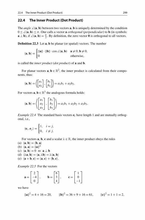
22.4 The Inner Product (Dot Product) 299
22.4 The Inner Product (Dot Product)
The angle �(a,b) between two vectors a,b is uniquely determined by the condition0 ≤ �(a,b) ≤ π . One calls a vector a orthogonal (perpendicular) to b (in symbols:a ⊥ b), if �(a,b) = π
2 . By definition, the zero vector 0 is orthogonal to all vectors.
Definition 22.3 Let a,b be planar (or spatial) vectors. The number
〈a,b〉 ={
‖a‖ · ‖b‖ · cos�(a,b) a = 0,b = 0,
0 otherwise,
is called the inner product (dot product) of a and b.
For planar vectors a,b ∈ R2, the inner product is calculated from their compo-
nents, thus:
〈a,b〉 =⟨[
a1a2
],
[b1b2
]⟩= a1b1 + a2b2.
For vectors a,b ∈ R3 the analogous formula holds:
〈a,b〉 =⟨⎡⎣a1
a2a3
⎤⎦ ,
⎡⎣b1
b2b3
⎤⎦
⟩= a1b1 + a2b2 + a3b3.
Example 22.4 The standard basis vectors ei have length 1 and are mutually orthog-onal, i.e.,
〈ei , ej 〉 ={
1, i = j,
0, i = j.
For vectors a, b, c and a scalar λ ∈ R, the inner product obeys the rules(a) 〈a,b〉 = 〈b,a〉(b) 〈a,a〉 = ‖a‖2
(c) 〈a,b〉 = 0 ⇔ a ⊥ b(d) 〈λa,b〉 = 〈a, λb〉 = λ〈a,b〉(e) 〈a + b, c〉 = 〈a, c〉 + 〈b, c〉.
Example 22.5 For the vectors
a =⎡⎣ 2
−40
⎤⎦ , b =
⎡⎣6
34
⎤⎦ , c =
⎡⎣ 1
0−1
⎤⎦
we have
‖a‖2 = 4 + 16 = 20, ‖b‖2 = 36 + 9 + 16 = 61, ‖c‖2 = 1 + 1 = 2,

300 22 Appendix A: Vector Algebra
and
〈a,b〉 = 12 − 12 = 0, 〈a, c〉 = 2.
From this we conclude that a is perpendicular to b and
cos�(a, c) = 〈a, c〉‖a‖ · ‖c‖ = 2√
20√
2= 1√
10.
The value of the angle between a and c is thus
�(a, c) = arccos1√10
= 1.249 rad.
22.5 The Outer Product (Cross Product)
For vectors a,b in R2 one defines
a × b =[a1a2
]×
[b1b2
]= det
[a1 b1a2 b2
]= a1b2 − a2b1 ∈ R,
the cross product of a and b. An elementary calculation shows that
|a × b| = ‖a‖ · ‖b‖ · sin�(a,b).
Thus |a × b| is the area of the parallelogram spanned by a and b.For vectors a,b ∈ R
3 one defines the cross product by
a × b =⎡⎣a1
a2a3
⎤⎦ ×
⎡⎣b1
b2b3
⎤⎦ =
⎡⎣a2b3 − a3b2
a3b1 − a1b3a1b2 − a2b1
⎤⎦ ∈ R
3.
This product has the following geometric interpretation: If a = 0 or b = 0 or a = λbthen a × b = 0. Otherwise a × b is the vector(a) which is perpendicular to a and b: 〈a × b,a〉 = 〈a × b,b〉 = 0(b) which is directed such that a,b,a × b forms a right-handed system(c) whose length is equal to the area F of the parallelogram spanned by a and b:
F = ‖a × b‖ = ‖a‖ · ‖b‖ · sin�(a,b).
Example 22.6 Let E be the plane spanned by the two vectors
a =⎡⎣ 1
−12
⎤⎦ and b =
⎡⎣1
01
⎤⎦ .
22.6 Straight Lines in the Plane 301
Then
a × b =⎡⎣ 1
−12
⎤⎦ ×
⎡⎣1
01
⎤⎦ =
⎡⎣−1
11
⎤⎦
is a vector perpendicular to this plane.
For a,b, c ∈ R3 and λ ∈ R, the following rules apply:
(a) a × a = 0, a × b = −(b × a)
(b) λ(a × b) = (λa) × b = a × (λb)
(c) (a + b) × c = a × c + b × c.However, the cross product is not associative and
a × (b × c) = (a × b) × c
for general a, b, c. For instance, the standard basis vectors of the R3 satisfy the
following identities:
e1 × (e1 × e2) = e1 × e3 = −e2,
(e1 × e1) × e2 = 0 × e2 = 0.
22.6 Straight Lines in the Plane
The general equation of a straight line in the (x, y)-plane is
ax + by = c,
where at least one of the coefficients a and b must be different from zero. Thestraight line consists of all points (x, y) which satisfy the above equation,
g = {(x, y) ∈ R
2; ax + by = c}.
If b = 0 (and thus a = 0) we get
x = c
a,
and thus a line parallel to the y-axis. If b = 0, one can solve for y and obtains thestandard form of a straight line:
y = −a
bx + c
b= kx + d
with slope k and intercept d .

302 22 Appendix A: Vector Algebra
The parametric representation of the straight line is obtained from the generalsolution of the linear equation
ax + by = c.
Since this equation is underdetermined, one replaces the independent variable by aparameter and solves for the other variable.
Example 22.7 In the equation
y = kx + d
x is considered as independent variable. One sets x = λ, and one obtains y = kλ+d
and thus the parametric representation
[x
y
]=
[0d
]+ λ
[1k
], λ ∈ R.
Example 22.8 In the equation
x = 4
y is the independent variable (it does not even appear). This straight line in para-metric representation is
[x
y
]=
[40
]+ λ
[01
].
In general, the parametric representation of a straight line is of the form
[x
y
]=
[p
q
]+ λ
[u
v
], λ ∈ R
(position vector of a point plus a multiple of a direction vector). A vector perpen-dicular to this straight line is called a normal vector. It is a multiple of
[v
−u
], since
⟨[u
v
],
[v
−u
]⟩= 0.
The conversion to the nonparametric form is obtained by multiplying the equationin parametric form by a normal vector. Thereby the parameter is eliminated. In theexample above one obtains
vx − uy = pv − qu.
In particular, the coefficients of x and y in the nonparametric form are just thecomponents of a normal vector of the straight line.

22.7 Planes in Space 303
22.7 Planes in Space
The general form of a plane in R3 is
ax + by + cz = d,
where at least one of the coefficients a, b, c is different from zero. The plane consistsof all points which satisfy the above equation, i.e.,
E = {(x, y, z) ∈ R
3; ax + by + cz = d}.
Since at least one of the coefficients is nonzero, one can solve the equation for thecorresponding unknown.
For example, if c = 0 one can solve for z to obtain
z = −a
cx − b
cy + d
c= kx + ly + e.
Here k represents the slope in the x-direction, l is the slope in the y-direction and e
the intercept on the z-axis (because z = e for x = y = 0). By introducing parametersfor the independent variables x and y,
x = λ, y = μ, z = kλ + lμ + e,
one thus obtains the parametric representation of the plane:
⎡⎣x
y
z
⎤⎦ =
⎡⎣0
0e
⎤⎦ + λ
⎡⎣1
0k
⎤⎦ + μ
⎡⎣0
1l
⎤⎦ , λ,μ ∈ R.
In general, the parametric representation of a plane in R3 is
⎡⎣x
y
z
⎤⎦ =
⎡⎣p
q
r
⎤⎦ + λ
⎡⎣v1
v2v3
⎤⎦ + μ
⎡⎣w1
w2w3
⎤⎦
with v × w = 0. If one multiplies this equation with v × w and uses
〈v,v × w〉 = 〈w,v × w〉 = 0,
one again obtains the nonparametric form
⟨⎡⎣x
y
z
⎤⎦ ,v × w
⟩=
⟨⎡⎣p
q
r
⎤⎦ ,v × w
⟩.

304 22 Appendix A: Vector Algebra
Example 22.9 We compute the nonparametric form of the plane
⎡⎣x
y
z
⎤⎦ =
⎡⎣3
11
⎤⎦ + λ
⎡⎣ 1
−12
⎤⎦ + μ
⎡⎣1
01
⎤⎦ .
A normal vector to this plane is given by
v × w =⎡⎣ 1
−12
⎤⎦ ×
⎡⎣1
01
⎤⎦ =
⎡⎣−1
11
⎤⎦ ,
and thus the equation of the plane is
−x + y + z = −1.
22.8 Straight Lines in Space
A straight line in R3 can be seen as the intersection of two planes:
g :{
ax + by + cz = d,
ex + fy + gz = h.
The straight line is the set of all points (x, y, z) which fulfill this system of equations(two equations in three unknowns). Generically, the solution of the above systemcan be parametrised by one parameter (this is the case of a straight line). However,it may also happen that the planes are parallel. In this situation they either coincide,or they do not intersect at all.
A straight line can also be represented parametrically by the position vector of apoint and an arbitrary multiple of a direction vector:
⎡⎣x
y
z
⎤⎦ =
⎡⎣p
q
r
⎤⎦ + λ
⎡⎣u
v
w
⎤⎦ , λ ∈ R.
The direction vector is obtained as difference of the position vectors of two pointson the straight line.
Example 22.10 We want to determine the straight line through the points P =(1,2,0) and Q = (3,1,2). A direction vector a of this line is given by
a =⎡⎣3
12
⎤⎦ −
⎡⎣1
20
⎤⎦ =
⎡⎣ 2
−12
⎤⎦ .

22.8 Straight Lines in Space 305
Thus a parametric representation of the straight line is
g :⎡⎣x
y
z
⎤⎦ =
⎡⎣1
20
⎤⎦ + λ
⎡⎣ 2
−12
⎤⎦ , λ ∈ R.
The conversion from parametric to nonparametric form and vice versa is achievedby elimination or introduction of a parameter λ. In the example above one computesz = 2λ from the last equation and inserts it into the first two equations. This yieldsthe nonparametric form
x − z = 1,
2y + z = 4.

23Appendix B: Matrices
In this book matrix algebra is required in multi-dimensional calculus, for systems ofdifferential equations and for linear regression. This appendix serves to outline thebasic notions. A more detailed presentation can be found in [2].
23.1 Matrix Algebra
An (m × n)-matrix A is a rectangular scheme of the form
A =
⎡⎢⎢⎢⎢⎣
a11 a12 . . . a1n
a21 a22 . . . a2n
......
...
am1 am2 . . . amn
⎤⎥⎥⎥⎥⎦ .
The entries (coefficients, elements) aij , i = 1, . . . ,m, j = 1, . . . , n of the matrix Aare real or complex numbers. In this section we restrict ourselves to real numbers.An (m×n)-matrix has m rows and n columns; if m = n, the matrix is called square.Vectors of length m can be understood as matrices with one column, i.e. as (m× 1)-matrices. In particular, one refers to the columns
aj =
⎡⎢⎢⎢⎣
a1j
a2j
...
amj
⎤⎥⎥⎥⎦ , j = 1, . . . , n,
of a matrix A as column vectors and accordingly also writes
A = [a1...a2
... . . ....an]
for the matrix. The rows of the matrix are sometimes called row vectors.
M. Oberguggenberger, A. Ostermann, Analysis for Computer Scientists,Undergraduate Topics in Computer Science,DOI 10.1007/978-0-85729-446-3_23, © Springer-Verlag London Limited 2011
307
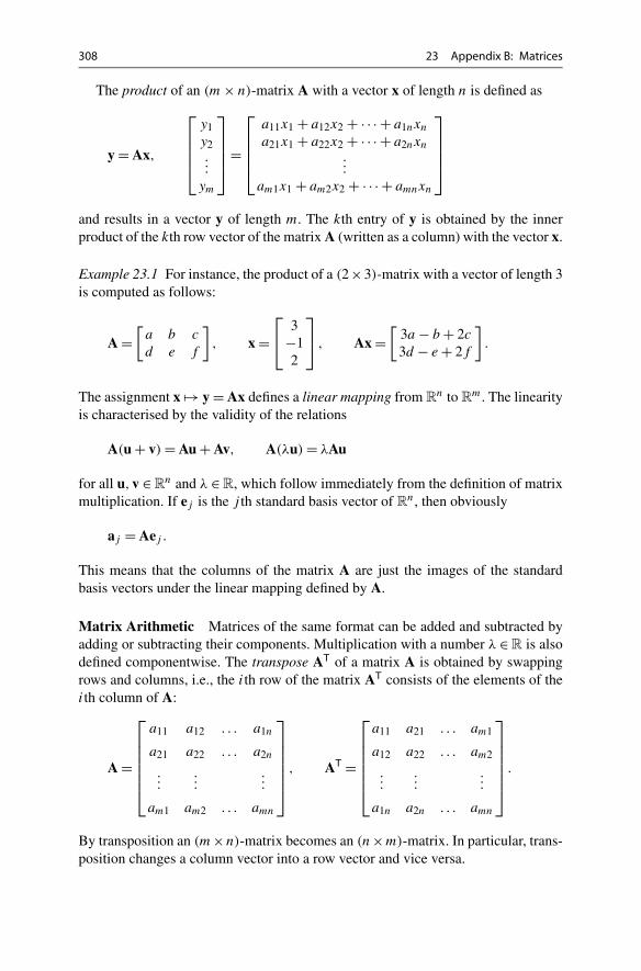
308 23 Appendix B: Matrices
The product of an (m × n)-matrix A with a vector x of length n is defined as
y = Ax,
⎡⎢⎢⎢⎣
y1y2...
ym
⎤⎥⎥⎥⎦ =
⎡⎢⎢⎢⎣
a11x1 + a12x2 + · · · + a1nxn
a21x1 + a22x2 + · · · + a2nxn
...
am1x1 + am2x2 + · · · + amnxn
⎤⎥⎥⎥⎦
and results in a vector y of length m. The kth entry of y is obtained by the innerproduct of the kth row vector of the matrix A (written as a column) with the vector x.
Example 23.1 For instance, the product of a (2×3)-matrix with a vector of length 3is computed as follows:
A =[
a b c
d e f
], x =
⎡⎣ 3
−12
⎤⎦ , Ax =
[3a − b + 2c
3d − e + 2f
].
The assignment x �→ y = Ax defines a linear mapping from Rn to R
m. The linearityis characterised by the validity of the relations
A(u + v) = Au + Av, A(λu) = λAu
for all u,v ∈ Rn and λ ∈ R, which follow immediately from the definition of matrix
multiplication. If ej is the j th standard basis vector of Rn, then obviously
aj = Aej .
This means that the columns of the matrix A are just the images of the standardbasis vectors under the linear mapping defined by A.
Matrix Arithmetic Matrices of the same format can be added and subtracted byadding or subtracting their components. Multiplication with a number λ ∈ R is alsodefined componentwise. The transpose AT of a matrix A is obtained by swappingrows and columns, i.e., the ith row of the matrix AT consists of the elements of theith column of A:
A =
⎡⎢⎢⎢⎢⎢⎣
a11 a12 . . . a1n
a21 a22 . . . a2n
......
...
am1 am2 . . . amn
⎤⎥⎥⎥⎥⎥⎦
, AT =
⎡⎢⎢⎢⎢⎢⎣
a11 a21 . . . am1
a12 a22 . . . am2
......
...
a1n a2n . . . amn
⎤⎥⎥⎥⎥⎥⎦
.
By transposition an (m×n)-matrix becomes an (n×m)-matrix. In particular, trans-position changes a column vector into a row vector and vice versa.

23.1 Matrix Algebra 309
Example 23.2 For the matrix A and the vector x from Example 23.1, we have
AT =⎡⎣a d
b e
c f
⎤⎦ , xT = [3 − 1 2], x = [3 − 1 2]T.
If a,b are vectors of length n, then one can regard aT as a (1 × n)-matrix. Itsproduct with the vector b is defined as above and coincides with the inner product:
aTb =n∑
i=1
aibi = 〈a,b〉.
More generally, the product of an (m × n)-matrix A with an (n × l)-matrix B canbe defined by forming the inner products of the row vectors of A with the columnvectors of B. This means that the element cij in the ith row and j th column ofC = AB is obtained by inner multiplication of the ith row of A with the j th columnof B:
cij =n∑
k=1
aikbkj .
The result is an (m× l)-matrix. The product is only defined if the dimensions match,i.e., if the number of columns n of A is equal to the number of rows of B. The matrixproduct corresponds to the composition of linear mappings. If B is the matrix of alinear mapping R
l → Rn and A the matrix of a linear mapping R
n → Rm, then AB
is just the matrix of the composition of the two mappings Rl → R
n → Rm. The
transposition of the product is given by the formula
(AB)T = BTAT,
which can easily be deduced from the definitions.
Square Matrices The entries a11, a22, . . . , ann of an (n × n)-matrix A are calledthe diagonal elements. A square matrix D is called a diagonal matrix, if its entriesare all zero with the possible exception of the diagonal elements. Special cases arethe zero matrix and the unit matrix of dimension n × n:
O =
⎡⎢⎢⎢⎣
0 0 . . . 00 0 . . . 0...
.... . .
...
0 0 . . . 0
⎤⎥⎥⎥⎦ , I =
⎡⎢⎢⎢⎣
1 0 . . . 00 1 . . . 0...
.... . .
...
0 0 . . . 1
⎤⎥⎥⎥⎦ .
The unit matrix is the identity with respect to matrix multiplication. For all (n × n)-matrices A the following holds: IA = AI = A. If for a given matrix A there exists amatrix B with the property
BA = AB = I,
310 23 Appendix B: Matrices
then one calls A invertible or regular and B the inverse of A, denoted by
B = A−1.
Let x ∈ Rn, A an invertible (n × n)-matrix and y = Ax. Then x can be computed
as x = A−1y; in particular, A−1Ax = x and AA−1y = y. This shows that the linearmapping R
n → Rn induced by the matrix A is bijective and A−1 represents the in-
verse mapping. The bijectivity of A can be expressed in yet another way. Bijectivitymeans that for every y ∈ R
n there is one and only one x ∈ Rn such that
Ax = y, or
a11x1 + a12x2 + · · · + a1nxn = y1,
a21x1 + a22x2 + · · · + a2nxn = y2,...
......
...
am1x1 + am2x2 + · · · + amnxn = yn.
The latter can be considered as a linear system of equations with right-hand sidey and solution x = [x1 x2 . . . xn]T. In other words, invertibility of a matrix A isequivalent to bijectivity of the corresponding linear mapping and equivalent withthe unique solvability of the corresponding linear system of equations (for arbitraryright-hand sides).
For the remainder of this appendix we restrict our attention to (2 × 2)-matrices.Let A be a (2 × 2)-matrix with the corresponding system of equations:
A = [a1...a2] =
[a11 a12a21 a22
],
a11x1 + a12x2 = y1,
a21x1 + a22x2 = y2.
An important role is played by the determinant of the matrix A. In the (2 × 2)-caseit is defined as the cross product of the column vectors:
det A = a1 × a2 = a11a22 − a21a12.
Since a1 × a2 = ‖a1‖‖a2‖ sin�(a1,a2), the column vectors a1,a2 are linearly de-pendent (so—in R
2—multiples of each other), if and only if det A = 0. The follow-ing theorem characterises invertibility in the (2 × 2)-case completely.
Proposition 23.3 For (2 × 2)-matrices A the following statements are equivalent:(a) A is invertible.(b) The linear mapping R
2 → R2 defined by A is bijective.
(c) The linear system of equations Ax = y has a unique solution x ∈ R2 for arbi-
trary right-hand sides y ∈ R2.
(d) The column vectors of A are linearly independent.(e) The linear mapping R
2 → R2 defined by A is injective.
(f) The only solution of the linear system of equations Ax = 0 is the zero solutionx = 0.
(g) det A �= 0.

23.2 Canonical Form of Matrices 311
Proof The equivalence of the statements (a), (b) and (c) was already observedabove. The equivalence of (d), (e) and (f) can easily be seen by negation. Indeed, ifthe column vectors are linearly dependent, then there exists x = [x1 x2]T �= 0 withx1a1 +x2a2 = 0. On the one hand, this means that the vector x is mapped to 0 by A,thus this mapping is not injective. On the other hand, x is a nontrivial solution of thelinear system of equations Ax = 0. The converse implications are shown in the sameway. Thus (d), (e) and (f) are equivalent. The equivalence of (g) and (d) is obviousfrom the geometric meaning of the determinant. If the determinant does not vanish,then
A−1 = 1
a11a22 − a21a12
[a22 −a12
−a21 a11
]
is an inverse to A, as can be verified at once. Thus (g) implies (a). Finally, (e) obvi-ously follows from (b). Hence all statements (a)–(g) are equivalent. �
Proposition 23.3 holds for matrices of arbitrary dimension n × n. For n = 3 onecan still use geometrical arguments. The cross product, however, has to be replacedby the triple product 〈a1 × a2,a3〉 of the three column vectors, which then alsodefines the determinant of the (3 × 3)-matrix A. In higher dimensions the proofrequires tools from combinatorics, for which we refer to the literature.
23.2 Canonical Form of Matrices
In this subsection we will show that every (2 × 2)-matrix A is similar to a matrix ofstandard type, which means that it can be put into standard form by a basis transfor-mation. We need this fact in Sect. 20.1 for the classification and solution of systemsof differential equations. The transformation explained below is a special case of theJordan canonical form1 for (n × n)-matrices.
If T is an invertible (2 × 2)-matrix, then the columns t1, t2 form a basis of R2.
This means that every element x ∈ R2 can be written in a unique way as a linear
combination c1t1 + c2t2; the coefficients c1, c2 ∈ R are the coordinates of x withrespect to t1 and t2. One can regard T as a linear transformation of R
2 which mapsthe standard basis {[1 0]T, [0 1]T} to the basis {t1, t2}.
Definition 23.4 Two matrices A,B are called similar, if there exists an invertiblematrix T such that T−1AT = B.
1C. Jordan, 1838–1922.

312 23 Appendix B: Matrices
The three standard types which will define the similarity classes of (2 × 2)-matricesare of the following form:
type I type II type III[λ1 00 λ2
] [λ 10 λ
] [μ −ν
ν μ
]
Here the coefficients λ1, λ2, λ,μ, ν are real numbers.In what follows, we need the notion of eigenvalues and eigenvectors. If the equa-
tion
Av = λv
has a solution v �= 0 ∈ R2 for some λ ∈ R, then λ is called eigenvalue and v eigen-
vector of A. In other words, v is a solution of the equation
(A − λI)v = 0,
where I denotes again the unit matrix. For the existence of a nonzero solution v it isnecessary and sufficient that the matrix A − λI is not invertible, i.e.,
det(A − λI) = 0.
By writing
A =[a b
c d
],
we see that λ has to be a solution of the characteristic equation:
det
[a − λ b
c d − λ
]= λ2 − (a + d)λ + ad − bc = 0.
If this equation has a real solution λ, then the system of equations (A − λI)v = 0 isunderdetermined and thus has a nonzero solution v = [v1 v2]T. Hence one obtainsthe eigenvectors to the eigenvalue λ by solving the linear system
(a − λ)v1 + bv2 = 0,
cv1 + (d − λ)v2 = 0.
Depending on whether the characteristic equation has two real, a double real or twocomplex conjugate solutions, we obtain one of the three similarity classes of A.
Proposition 23.5 Every (2 × 2)-matrix A is similar to a matrix of type I, II or III.
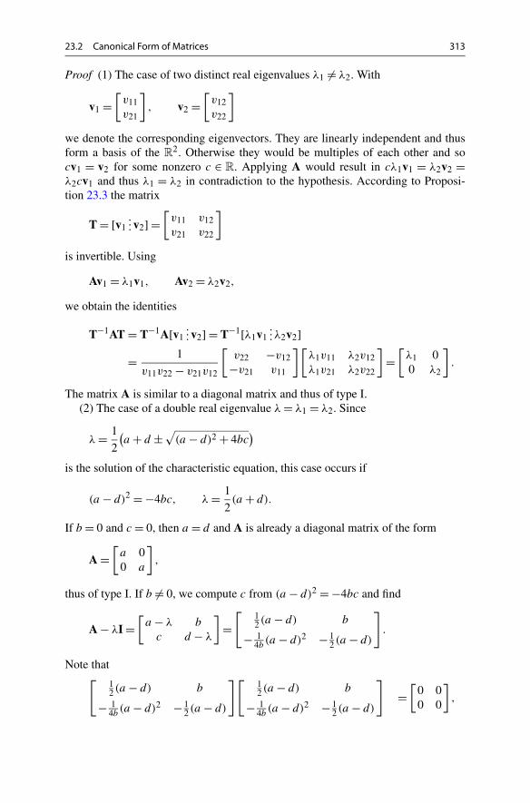
23.2 Canonical Form of Matrices 313
Proof (1) The case of two distinct real eigenvalues λ1 �= λ2. With
v1 =[v11v21
], v2 =
[v12v22
]
we denote the corresponding eigenvectors. They are linearly independent and thusform a basis of the R
2. Otherwise they would be multiples of each other and socv1 = v2 for some nonzero c ∈ R. Applying A would result in cλ1v1 = λ2v2 =λ2cv1 and thus λ1 = λ2 in contradiction to the hypothesis. According to Proposi-tion 23.3 the matrix
T = [v1...v2] =
[v11 v12v21 v22
]
is invertible. Using
Av1 = λ1v1, Av2 = λ2v2,
we obtain the identities
T−1AT = T−1A[v1...v2] = T−1[λ1v1
... λ2v2]= 1
v11v22 − v21v12
[v22 −v12
−v21 v11
][λ1v11 λ2v12λ1v21 λ2v22
]=
[λ1 00 λ2
].
The matrix A is similar to a diagonal matrix and thus of type I.(2) The case of a double real eigenvalue λ = λ1 = λ2. Since
λ = 1
2
(a + d ±
√(a − d)2 + 4bc
)
is the solution of the characteristic equation, this case occurs if
(a − d)2 = −4bc, λ = 1
2(a + d).
If b = 0 and c = 0, then a = d and A is already a diagonal matrix of the form
A =[a 00 a
],
thus of type I. If b �= 0, we compute c from (a − d)2 = −4bc and find
A − λI =[a − λ b
c d − λ
]=
[12 (a − d) b
− 14b
(a − d)2 − 12 (a − d)
].
Note that[12 (a − d) b
− 14b
(a − d)2 − 12 (a − d)
][12 (a − d) b
− 14b
(a − d)2 − 12 (a − d)
]=
[0 00 0
],
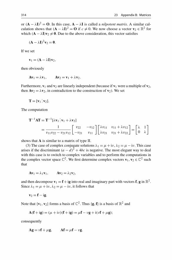
314 23 Appendix B: Matrices
or (A − λI)2 = O. In this case, A − λI is called a nilpotent matrix. A similar cal-culation shows that (A − λI)2 = O if c �= 0. We now choose a vector v2 ∈ R
2 forwhich (A − λI)v2 �= 0. Due to the above consideration, this vector satisfies
(A − λI)2v2 = 0.
If we set
v1 = (A − λI)v2,
then obviously
Av1 = λv1, Av2 = v1 + λv2.
Furthermore, v1 and v2 are linearly independent (because if v1 were a multiple of v2,then Av2 = λv2, in contradiction to the construction of v2). We set
T = [v1...v2].
The computation
T−1AT = T−1[λv1...v1 + λv2]
= 1
v11v22 − v21v12
[v22 −v12
−v21 v11
][λv11 v11 + λv12
λv21 v21 + λv22
]=
[λ 10 λ
]
shows that A is similar to a matrix of type II.(3) The case of complex conjugate solutions λ1 = μ+ iν, λ2 = μ− iν. This case
arises if the discriminant (a − d)2 + 4bc is negative. The most elegant way to dealwith this case is to switch to complex variables and to perform the computations inthe complex vector space C
2. We first determine complex vectors v1,v2 ∈ C2 such
that
Av1 = λ1v1, Av2 = λ2v2,
and then decompose v1 = f + ig into real and imaginary part with vectors f, g in R2.
Since λ1 = μ + iν, λ2 = μ − iν, it follows that
v2 = f − ig.
Note that {v1,v2} forms a basis of C2. Thus {g, f} is a basis of R
2 and
A(f + ig) = (μ + iν)(f + ig) = μf − νg + i(νf + μg);consequently
Ag = νf + μg, Af = μf − νg.
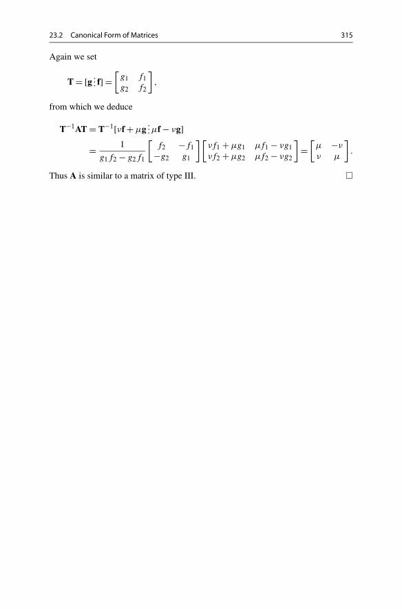
23.2 Canonical Form of Matrices 315
Again we set
T = [g ... f] =[g1 f1g2 f2
],
from which we deduce
T−1AT = T−1[νf + μg...μf − νg]
= 1
g1f2 − g2f1
[f2 −f1
−g2 g1
][νf1 + μg1 μf1 − νg1νf2 + μg2 μf2 − νg2
]=
[μ −ν
ν μ
].
Thus A is similar to a matrix of type III. �

24Appendix C: Further Results on Continuity
This appendix covers further material on continuity which is not central for this bookbut on the other hand is required in various proofs (like, for instance, in the chapterson curves and differential equations). It includes assertions about the continuity ofthe inverse function, the concept of uniform convergence of sequences of functions,the power series expansion of the exponential function and the notions of uniformand Lipschitz continuity.
24.1 Continuity of the Inverse Function
We consider a real-valued function f defined on an interval I ⊂ R. The interval I
can be open, half-open or closed. By J = f (I) we denote the image of f . First, weshow that a continuous function f : I → J is bijective, if and only if it is strictlymonotonically increasing or decreasing. Monotonicity was introduced in Defini-tion 8.5. Subsequently, we show that the inverse function is continuous if f is con-tinuous, and we describe the respective ranges.
Proposition 24.1 A real-valued, continuous function f : I → J = f (I) is bijectiveif and only if it is strictly monotonically increasing or decreasing.
Proof We already know that the function f : I → f (I) is surjective. It is injectiveif and only if
x1 �= x2 ⇒ f (x1) �= f (x2).
Strict monotonicity thus implies injectivity. To prove the converse implication westart by choosing two points x1 < x2 ∈ I . Let f (x1) < f (x2), for example. Wewill show that f is strictly monotonically increasing on the entire interval I . Firstwe observe that for every x3 ∈ (x1, x2) we must have f (x1) < f (x3) < f (x2).This is shown by contradiction. Assuming f (x3) > f (x2), Proposition 6.14 im-plies that every intermediate point f (x2) < η < f (x3) would be the image of a
M. Oberguggenberger, A. Ostermann, Analysis for Computer Scientists,Undergraduate Topics in Computer Science,DOI 10.1007/978-0-85729-446-3_24, © Springer-Verlag London Limited 2011
317

318 24 Appendix C: Further Results on Continuity
point ξ1 ∈ (x1, x3) and also the image of a point ξ2 ∈ (x3, x2), contradicting injec-tivity.
If we now choose x4 ∈ I such that x2 < x4, then once again f (x2) < f (x4).Otherwise we would have x1 < x2 < x4 with f (x2) > f (x4); this possibility is ex-cluded as in the previous case. Finally, the points to the left of x1 are inspected in asimilar way. It follows that f is strictly monotonically increasing on the entire inter-val I . In the case f (x1) > f (x2), one can deduce similarly that f is monotonicallydecreasing. �
The function y = x · 1(−1,0](x) + (1 − x) · 1(0,1)(x), where 1I denotes the indi-cator function of the interval I (see Sect. 2.2), shows that a discontinuous functioncan be bijective on an interval without being strictly monotonically increasing ordecreasing.
Remark 24.2 If I is an open interval and f : I → J a continuous and bijectivefunction, then J is an open interval as well. Indeed, if J were of the form [a, b),then a would arise as function value of a point x1 ∈ I , i.e. a = f (x1). However,since I is open, there are points x2 ∈ I , x2 < x1 and x3 ∈ I with x3 > x1. If f isstrictly monotonically increasing then we would have f (x2) < f (x1) = a. If f isstrictly monotonically decreasing then f (x3) < f (x1) = a. Both cases contradictthe fact that a was assumed to be the lower boundary of the image J = f (I). In thesame way, one excludes the possibilities that J = (a, b] or J = [a, b].
Proposition 24.3 Let I ⊂ R be an open interval and f : I → J continuous andbijective. Then the inverse function f −1 : J → I is continuous as well.
Proof We take x ∈ I , y ∈ J with y = f (x), x = f −1(y). For small ε > 0 theε-neighbourhood Uε(x) of x is contained in I . According to Remark 24.2 f (Uε(x))
is an open interval and therefore contains a δ-neighbourhood Uδ(y) of y for a certainδ > 0. Consider a sequence of values yn ∈ J which converges to y as n → ∞. Thenthere is an index n(δ) ∈ N such that all elements of the sequence yn with n ≥ n(δ)
lie in the δ-neighbourhood Uδ(y). This, however, means that the values of the func-tion f −1(yn) from n(δ) onwards lie in the ε-neighbourhood Uε(x) of x = f −1(y).Thus limn→∞ f −1(yn) = f −1(y) which is the continuity of f −1 at y. �
24.2 Limits of Sequences of Functions
We consider a sequence of functions fn : I → R, defined on an interval I ⊂ R. Ifthe function values fn(x) converge for every fixed x ∈ I , then the sequence (fn)n≥1
is called pointwise convergent. The pointwise limits define a function f : I → R byf (x) = limn→∞ fn(x), the so-called limit function.
24.2 Limits of Sequences of Functions 319
Example 24.4 Let I = [0,1] and fn(x) = xn. Then limn→∞ fn(x) = 0 if 0 ≤ x < 1,and limn→∞ fn(1) = 1. The limit function is thus the function
f (x) ={
0, 0 ≤ x < 1,
1, x = 1.
This example shows that the limit function of a pointwise convergent sequence ofcontinuous functions is not necessarily continuous.
Definition 24.5 (Uniform convergence of sequences of functions) A sequence offunctions (fn)n≥1 defined on an interval I is called uniformly convergent with limitfunction f , if
∀ε > 0 ∃n(ε) ∈ N ∀n ≥ n(ε) ∀x ∈ I : ∣∣f (x) − fn(x)∣∣ < ε.
Uniform convergence means that the index n(ε) after which the sequence offunction values (fn(x))n≥1 settles in the ε-neighbourhood Uε(f (x)) can be chosenindependently of x ∈ I .
Proposition 24.6 The limit function f of a uniformly convergent sequence of func-tions (fn)n≥1 is continuous.
Proof We take x ∈ I and a sequence of points xk converging to x as k → ∞. Wehave to show that f (x) = limk→∞ f (xk). For this we write
f (x) − f (xk) = (f (x) − fn(x)
) + (fn(x) − fn(xk)
) + (fn(xk) − f (xk)
)and choose ε > 0. Due to the uniform convergence it is possible to find an indexn ∈ N such that∣∣f (x) − fn(x)
∣∣ <ε
3and
∣∣fn(xk) − f (xk)∣∣ <
ε
3
for all k ∈ N. Since fn is continuous, there is an index k(ε) ∈ N such that
∣∣fn(x) − fn(xk)∣∣ <
ε
3
for all k ≥ k(ε). For such indices k we have
∣∣f (x) − f (xk)∣∣ <
ε
3+ ε
3+ ε
3= ε.
Thus f (xk) → f (x) as k → ∞, which implies the continuity of f . �
Application 24.7 The exponential function f (x) = ax is continuous on R. In Ap-plication 5.14 it was shown that the exponential function with base a > 0 can bedefined for every x ∈ R as a limit. Let rn(x) denote the decimal representation of x,truncated at the nth decimal place. Then
rn(x) ≤ x < rn(x) + 10−n.

320 24 Appendix C: Further Results on Continuity
The value of rn(x) is the same for all real numbers x, which coincide up to thenth decimal place. Thus the mapping x �→ rn(x) is a step function with jumps at adistance of 10−n. We define the function fn(x) by linear interpolation between thepoints
(rn(x), arn(x)
)and
(rn(x) + 10−n, arn(x)+10−n)
,
which means
fn(x) = arn(x) + x − rn(x)
10−n
(arn(x)+10−n − arn(x)
).
The graph of the function fn(x) is a polygonal chain (with kinks at the distance of10−n), and thus fn is continuous. We show that the sequence of functions (fn)n≥1converges uniformly to f on every interval [−T ,T ], 0 < T ∈ Q. Since x − rn(x) ≤10−n, it follows that∣∣f (x) − fn(x)
∣∣ ≤ ∣∣ax − arn(x)∣∣ + ∣∣arn(x)+10−n − arn(x)
∣∣.For x ∈ [−T ,T ] we have
ax − arn(x) = arn(x)(ax−rn(x) − 1
) ≤ aT(a10−n − 1
)and likewise
arn(x)+10−n − arn(x) ≤ aT(a10−n − 1
).
Consequently∣∣f (x) − fn(x)∣∣ ≤ 2aT
(10n√
a − 1),
and the term on the right-hand side converges to zero independently of x, as wasproven in Application 5.15.
The rules of calculation for real exponents can now also be derived by takinglimits. Take, for example, r, s ∈ R with decimal approximations (rn)n≥1, (sn)n≥1.Then Proposition 5.7 and the continuity of the exponential function imply
aras = limn→∞
(arnasn
) = limn→∞
(arn+sn
) = ar+s .
With the help of Proposition 24.3 the continuity of the logarithm follows as well.
24.3 The Exponential Series
The aim of this section is to derive the series representation of the exponential func-tion
ex =∞∑
m=0
xm
m!
24.3 The Exponential Series 321
by using exclusively the theory of convergent series without resorting to differentialcalculus. This is important for our exposition because the differentiability of theexponential function is proven with the help of the series representation in Sect. 7.2.
As a tool we need two supplements to the theory of series: absolute convergenceand Cauchy’s1 formula for the product of two series.
Definition 24.8 A series∑∞
k=0 ak is called absolutely convergent, if the series∑∞k=0 |ak| of the absolute values of its coefficients converges.
Proposition 24.9 Every absolutely convergent series is convergent.
Proof We define the positive and the negative part of the coefficient ak by
a+k =
{ak, ak ≥ 0,
0, ak < 0,a−k =
{0, ak ≥ 0,
|ak|, ak < 0.
Obviously, we have 0 ≤ a+k ≤ |ak| and 0 ≤ a−
k ≤ |ak|. Thus, the two series∑∞
k=0 a+k
and∑∞
k=0 a−k converge due to the comparison criterion (Proposition 5.21) and the
limit
limn→∞
n∑k=0
ak = limn→∞
n∑k=0
a+k − lim
n→∞
n∑k=0
a−k
exists. Consequently, the series∑∞
k=0 ak converges. �
We consider two absolutely convergent series∑∞
i=0 ai and∑∞
j=0 bj and ask howtheir product can be computed. Term-by-term multiplication of the nth partial sumssuggests to consider the following scheme:
a0b0 a0b1 . . . a0bn−1 a0bn
a1b0 a1b1 . . . a1bn−1 a1bn
.... . .
...
an−1b0 an−1b1 . . . an−1bn−1 an−1bn
anb0 anb1 . . . anbn−1 anbn
Adding all entries of the quadratic scheme one obtains the product of the partialsums
Pn =n∑
i=0
ai
n∑j=0
bj .
1A.L. Cauchy, 1789–1857.

322 24 Appendix C: Further Results on Continuity
In contrast, adding only the upper triangle containing the bold entries (diagonal bydiagonal), one obtains the so-called Cauchy product formula
Sn =n∑
m=0
(m∑
k=0
akbm−k
).
We want to show that, for absolutely convergent series, the limits are equal:
limn→∞Pn = lim
n→∞Sn.
Proposition 24.10 (Cauchy product) If the series∑∞
i=0 ai and∑∞
j=0 bj convergeabsolutely, then
∞∑i=0
ai
∞∑j=0
bj =∞∑
m=0
(m∑
k=0
akbm−k
).
The series defined by the Cauchy product formula also converges absolutely.
Proof We set
cm =m∑
k=0
akbm−k
and obtain that the partial sums
Tn =n∑
m=0
|cm| ≤n∑
i=0
|ai |n∑
j=0
|bj | ≤∞∑i=0
|ai |∞∑
j=0
|bj |
remain bounded. This follows from the facts that the triangle in the scheme abovehas fewer entries than the square and the original series converge absolutely. Ob-viously the sequence Tn is also monotonically increasing; according to Proposi-tion 5.10 it thus has a limit. This means that the series
∑∞m=0 cm converges abso-
lutely, so the Cauchy product exists. It remains to be shown that it coincides withthe product of the series. For the partial sums, we have
|Pn − Sn| =∣∣∣∣∣
n∑i=0
ai
n∑j=0
bj −n∑
m=0
cm
∣∣∣∣∣ ≤∣∣∣∣∣
∞∑m=n+1
cm
∣∣∣∣∣,
since the difference can obviously be approximated by the sum of the terms belowthe nth diagonal. The latter sum, however, is just the difference of the partial sumSn and the value of the series
∑∞m=0 cm. It thus converges to zero and the desired
assertion is proven. �
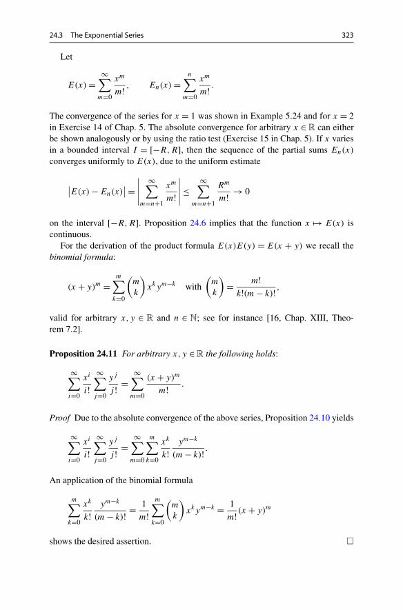
24.3 The Exponential Series 323
Let
E(x) =∞∑
m=0
xm
m! , En(x) =n∑
m=0
xm
m! .
The convergence of the series for x = 1 was shown in Example 5.24 and for x = 2in Exercise 14 of Chap. 5. The absolute convergence for arbitrary x ∈ R can eitherbe shown analogously or by using the ratio test (Exercise 15 in Chap. 5). If x variesin a bounded interval I = [−R,R], then the sequence of the partial sums En(x)
converges uniformly to E(x), due to the uniform estimate
∣∣E(x) − En(x)∣∣ =
∣∣∣∣∣∞∑
m=n+1
xm
m!
∣∣∣∣∣ ≤∞∑
m=n+1
Rm
m! → 0
on the interval [−R,R]. Proposition 24.6 implies that the function x �→ E(x) iscontinuous.
For the derivation of the product formula E(x)E(y) = E(x + y) we recall thebinomial formula:
(x + y)m =m∑
k=0
(m
k
)xkym−k with
(m
k
)= m!
k!(m − k)! ,
valid for arbitrary x, y ∈ R and n ∈ N; see for instance [16, Chap. XIII, Theo-rem 7.2].
Proposition 24.11 For arbitrary x, y ∈ R the following holds:
∞∑i=0
xi
i!∞∑
j=0
yj
j ! =∞∑
m=0
(x + y)m
m! .
Proof Due to the absolute convergence of the above series, Proposition 24.10 yields
∞∑i=0
xi
i!∞∑
j=0
yj
j ! =∞∑
m=0
m∑k=0
xk
k!ym−k
(m − k)! .
An application of the binomial formula
m∑k=0
xk
k!ym−k
(m − k)! = 1
m!m∑
k=0
(m
k
)xkym−k = 1
m! (x + y)m
shows the desired assertion. �

324 24 Appendix C: Further Results on Continuity
Proposition 24.12 (Series representation of the exponential function) The expo-nential function possesses the series representation
ex =∞∑
m=0
xm
m! ,
valid for arbitrary x ∈ R.
Proof By definition of the number e (see Example 5.24) we obviously have
e0 = 1 = E(0), e1 = e = E(1).
From Proposition 24.11 we get, in particular,
e2 = e1+1 = e1e1 = E(1)E(1) = E(1 + 1) = E(2)
and recursively
em = E(m) for m ∈ N.
The relation E(m)E(−m) = E(m − m) = E(0) = 1 shows that
e−m = 1
em= 1
E(m)= E(−m).
Likewise, one concludes from (E(1/n))n = E(1) that
e1/n = n√
e = n√
E(1) = E(1/n).
So far, this shows that ex = E(x) holds for all rational x = m/n. From Applica-tion 24.7 we know that the exponential function x �→ ex is continuous. The conti-nuity of the function x �→ E(x) was shown above. But two continuous functionswhich coincide for all rational numbers are equal. More precisely, if x ∈ R and xj
is the decimal expansion of x truncated at the j th place, then
ex = limj→∞ exj = lim
j→∞E(xj ) = E(x),
which is the desired result. �
Remark 24.13 The rigorous introduction of the exponential function is surprisinglyinvolved and is handled differently by different authors. The total effort, however, isapproximately the same in all approaches. We took the following route: introductionof Euler’s number e as the value of a convergent series (Example 5.24); definitionof the exponential function x �→ ex for x ∈ R by using the completeness of thereal numbers (Application 5.14); continuity of the exponential function based onuniform convergence (Application 24.7); series representation (Proposition 24.12);differentiability and calculation of the derivative (Sect. 7.2). Finally, in the courseof the computation of the derivative we also obtained the well-known formula e =limn→∞(1 + 1/n)n, which Euler himself used as a definition.

24.4 Lipschitz Continuity and Uniform Continuity 325
24.4 Lipschitz Continuity and Uniform Continuity
Some results on curves and differential equations require more refined continuityproperties. More precisely, methods for quantifying how the function values changein dependence on the arguments are needed.
Definition 24.14 A function f : D ⊂ R → R is called Lipschitz continuous, if thereexists a constant L > 0 such that the inequality
∣∣f (x1) − f (x2)∣∣ ≤ L|x1 − x2|
holds for all x1, x2 ∈ D. In this case L is called a Lipschitz constant of the func-tion f .
If x ∈ D and (xn)n≥1 is a sequence of points in D which converges to x, the in-equality |f (x) − f (xn)| ≤ L|x − xn| implies that f (xn) → f (x) as n → ∞. EveryLipschitz continuous function is thus continuous. For Lipschitz continuous func-tions one can quantify how much change in the x-values can be allowed to obtain achange in the function values of ε > 0 at the most:
|x1 − x2| < ε/L ⇒ ∣∣f (x1) − f (x2)∣∣ < ε.
Occasionally the following weaker quantification is required.
Definition 24.15 A function f : D ⊂ R → R is called uniformly continuous, ifthere exists a mapping ω : (0,1] → (0,1] : ε �→ ω(ε) such that
|x1 − x2| < ω(ε) ⇒ ∣∣f (x1) − f (x2)∣∣ < ε
for all x1, x2 ∈ D. In this case the mapping ω is called the modulus of continuity ofthe function f .
Every Lipschitz continuous function is uniformly continuous (with ω(ε) = ε/L),every uniformly continuous function is continuous.
Example 24.16 (a) The quadratic function f (x) = x2 is Lipschitz continuous onevery bounded interval [a, b]. For x1 ∈ [a, b] we have |x1| ≤ M = max(|a|, |b|) andlikewise for x2. Thus
∣∣f (x1) − f (x2)∣∣ = ∣∣x2
1 − x22
∣∣ = |x1 + x2||x1 − x2| ≤ 2M|x1 − x2|holds for all x1, x2 ∈ [a, b].
(b) The absolute value function f (x) = |x| is Lipschitz continuous on D = R
(with Lipschitz constant L = 1). This follows from the inequality∣∣|x1| − |x2|
∣∣ ≤ |x1 − x2|,which is valid for all x1, x2 ∈ R.
326 24 Appendix C: Further Results on Continuity
(c) The square root function f (x) = √x is uniformly continuous on the interval
[0,1], but not Lipschitz continuous. This follows from the inequality∣∣√x1 − √
x2∣∣ ≤ √|x1 − x2|,
which is proved immediately by squaring. Thus ω(ε) = ε2 is a modulus of continu-ity of the square root function on the interval [0,1]. The square root function is notLipschitz continuous on [0,1], since otherwise the choice x2 = 0 would imply therelations
√x1 ≤ L|x1|, 1√
x1≤ L,
which cannot hold for fixed L > 0 and all x1 ∈ (0,1].(d) The function f (x) = 1
xis continuous on the interval (0,1), but not uniformly
continuous. Assume that we could find a modulus of continuity ε �→ ω(ε) on (0,1).Then for x1 = 2εω(ε), x2 = εω(ε) and ε < 1 we would get |x1 − x2| < ω(ε), but
∣∣∣∣ 1
x1− 1
x2
∣∣∣∣ =∣∣∣∣x2 − x1
x1x2
∣∣∣∣ = εω(ε)
2ε2ω(ε)2= 1
2εω(ε)
which becomes arbitrarily large as ε → 0. In particular, it cannot be bounded fromabove by ε.
From the mean value theorem (Proposition 8.4) it follows that differentiablefunctions with bounded derivative are Lipschitz continuous. Further it can be shownthat every function which is continuous on a closed, bounded interval [a, b] is uni-formly continuous there. The proof requires further tools from analysis for whichwe refer to [4, Theorem 3.13].
Apart from the intermediate value theorem, the fixed point theorem is an impor-tant tool for proving the existence of solutions of equations. Moreover one obtainsan iterative algorithm for approximating the fixed point.
Definition 24.17 A Lipschitz continuous mapping f of an interval I to R is calleda contraction, if f (I) ⊂ I and f has a Lipschitz constant L < 1. A point x∗ ∈ I
with x∗ = f (x∗) is called fixed point of the function f .
Proposition 24.18 (Fixed point theorem) A contraction f on a closed interval[a, b] has a unique fixed point. The sequence, recursively defined by the iteration
xn+1 = f (xn)
converges to the fixed point x∗ for arbitrary initial values x1 ∈ [a, b].
Proof Since f ([a, b]) ⊂ [a, b] we must have
a ≤ f (a) and f (b) ≤ b.

24.4 Lipschitz Continuity and Uniform Continuity 327
If a = f (a) or b = f (b), we are done. Otherwise the intermediate value theoremapplied to the function g(x) = x − f (x) yields the existence of a point x∗ ∈ (a, b)
with g(x∗) = 0. This x∗ is a fixed point of f . Due to the contraction property theexistence of a further fixed point y∗ would result in
|x∗ − y∗| = ∣∣f (x∗) − f (y∗)∣∣ ≤ L|x∗ − y∗| < |x∗ − y∗|
which is impossible for x∗ �= y∗. Thus the fixed point is unique.The convergence of the iteration follows from the inequalities
|x∗ − xn+1| =∣∣f (x∗) − f (xn)
∣∣ ≤ L|x∗ − xn| ≤ · · · ≤ Ln|x∗ − x1|,since |x∗ − x1| ≤ b − a and limn→∞ Ln = 0. �

25Appendix D: Descriptionof the Supplementary Software
In our view using and writing software forms an essential component of an analysiscourse for computer scientists. The software that has been developed for this bookis available on the website
http://www.springer.com/978-0-85729-445-6.
This site contains the Java applets referred to in the text as well as some source filesin maple and MATLAB.
For the execution of the maple and MATLAB programs additional licenses areneeded. The use of the Java applets requires a plug-in for your browser.
Java Applets The available applets are listed in Table 25.1. For full functionalityof the applets, you need to activate JavaScript in your browser.
Table 25.1 Java appletsSequences
2D-visualisation of complex functions
3D-visualisation of complex functions
Bisection method
Animation of the intermediate value theorem
Newton’s method
Riemann sums
Integration
Parametric curves in the plane
Parametric curves in space
Surfaces in space
Dynamical systems in the plane
Dynamical systems in space
Linear regression
M. Oberguggenberger, A. Ostermann, Analysis for Computer Scientists,Undergraduate Topics in Computer Science,DOI 10.1007/978-0-85729-446-3_25, © Springer-Verlag London Limited 2011
329

330 25 Appendix D: Description of the Supplementary Software
Source Codes in MATLAB and maple In addition to the Java applets, you canfind maple and MATLAB programs on this website. These programs are numberedaccording to the individual chapters and are mainly used in experiments and exer-cises. To run the programs, the corresponding software license is required.
The Gallery in Maths Online At various places in the text, we refer to the galleryof maths online. This gallery was originally developed under the name mathe on-line as a web-based interactive learning aid for Austrian high schools and univer-sities by Franz Embacher and Petra Oberhuemer. The pages maths online are anEnglish translation, provided by the authors of mathe online. The gallery is freelyaccessible on the web
http://www.univie.ac.at/future.media/moe/.
Some elements of the gallery are referred to in experiments and exercises. We rec-ommend to use maths online for further practice as well.
References
Textbooks
1. E. HAIRER, G. WANNER: Analysis by Its History. Springer, New York 1996.2. S. LANG: Introduction to Linear Algebra. Springer, New York 1986 (2nd edition).3. S. LANG: Undergraduate Analysis. Springer, New York 1983.4. M.H. PROTTER, C.B. MORREY: A First Course in Real Analysis. Springer, New York 1991
(2nd edition).
Further Reading
5. M. BARNSLEY: Fractals Everywhere, Academic Press, Boston 1988.6. M. BRAUN, C.C. COLEMAN, D.A. DREW (Eds.): Differential Equation Models. Springer,
Berlin 1983.7. M. BRONSTEIN: Symbolic Integration I: Transcendental Functions. Springer, Berlin 1997.8. A. CHEVAN, M. SUTHERLAND: Hierarchical partitioning. The American Statistician 45
(1991), 90–96.9. J.P. ECKMANN: Savez-vous résoudre z3 = 1? La Recherche 14 (1983), 260–262.
10. N. FICKEL: Partition of the coefficient of determination in multiple regression. In: K. INDER-FURTH (Ed.), Operations Research Proceedings 1999, Springer, Berlin, 2000, 154–159.
11. E. HAIRER, S.P. NØRSETT, G. WANNER: Solving Ordinary Differential Equations I. NonstiffProblems. Springer, Berlin 1993 (2nd edition).
12. E. HAIRER, G. WANNER: Solving Ordinary Differential Equations II. Stiff and Differential-Algebraic Problems. Springer, Berlin 1996 (2nd edition).
13. M.W. HIRSCH, S. SMALE: Differential Equations, Dynamical Systems, and Linear Algebra.Academic Press, New York 1974.
14. E. KREYSZIG: Statistische Methoden und ihre Anwendungen. Vandenhoeck & Ruprecht, Göt-tingen 1968 (3rd edition).
15. W. KRUSKAL: Relative importance by averaging over orderings. The American Statistician41 (1987), 6–10.
16. S. LANG: A First Course in Calculus. Springer, New York 1986 (5th edition).17. M. LEFEBVRE: Basic Probability Theory with Applications. Springer, New York 2009.18. D.C. MONTGOMERY, E.A. PECK, G.G. VINING: Introduction to Linear Regression Analy-
sis. Wiley, New York 2001 (3rd edition).19. M.L. OVERTON: Numerical Computing with IEEE Floating Point Arithmetic. SIAM,
Philadelphia 2001.20. H.-O. PEITGEN, H. JÜRGENS, D. SAUPE: Fractals for the Classroom. Part One: Introduction
to Fractals and Chaos. Springer, New York 1992.21. H.-O. PEITGEN, H. JÜRGENS, D. SAUPE: Fractals for the Classroom. Part Two: Complex
Systems and Mandelbrot Set. Springer, New York 1992.
M. Oberguggenberger, A. Ostermann, Analysis for Computer Scientists,Undergraduate Topics in Computer Science,DOI 10.1007/978-0-85729-446-3, © Springer-Verlag London Limited 2011
331

332 References
22. A. QUARTERONI, R. SACCO, F. SALERI: Numerical Mathematics. Springer, New York 2000.23. H. ROMMELFANGER: Differenzen- und Differentialgleichungen. Bibliographisches Institut,
Mannheim 1977.24. STATISTIK AUSTRIA: Statistisches Jahrbuch Österreichs. Verlag Österreich GmbH, Wien
2007 (http://www.statistik.at).25. M.A. VÄTH: Nonstandard Analysis. Birkhäuser, Basel 2007.

Index
SymbolsC, 37N, 1N0, 1Q, 1R, 4Z, 1e, 22, 57, 77, 152, 289i, 37π , 3,28∇ , 204∞, 7
AAbsolute value, 7, 38
function, 19Acceleration, 81
vector, 175, 186Addition theorems, 30, 40, 77Affine function
derivative, 76Analysis of variance, 239Angle, between vectors, 299ANOVA, 239Antiderivative, 128Approximation
linear, 80, 201quadratic, 205
Arc length, 28, 180graph, 144parametrisation, 180
Arccosine, 32derivative, 86graph, 32
Archimedean spiral, 183Archimedes, 183Arcsine, 31
derivative, 86graph, 32
Arctangent, 32derivative, 86graph, 33
Areasector, 67surface of sphere, 145triangle, 27under a graph function, 136
Area element, 225Argument, 39Arithmetic of real numbers, 52Ascent, steepest, 204Axial moment, 230
BBasis, standard, 296Beam, 108Bijective, see functionBinomial formula, 323Binormal vector, 186Bisection method, 70, 100, 103Bolzano, B., 59, 68Bolzano–Weierstrass
theorem of, 59Box-dimension, 114
CCantor, G., 2
set, 115Cardioid, 184
parametric representation, 184Cauchy, A.L., 321
product, 322Cavalieri, B., 222Cavalieri’s principle, 222Centre of gravity, 226
geometric, 226Chain rule, 83, 200Characteristic equation, 312Circle
of latitude, 217
M. Oberguggenberger, A. Ostermann, Analysis for Computer Scientists,Undergraduate Topics in Computer Science,DOI 10.1007/978-0-85729-446-3, © Springer-Verlag London Limited 2011
333
334 Index
Circle (cont.)osculating, 182parametric representation, 170unit, 28
Circular arclength, 179
Clothoid, 182parametric representation, 182
Coastline, 114, 241Coefficient of determination, 240
multiple, 244partial, 246
Column vector, 307Completeness, 2, 51Complex conjugate, 38Complex exponential function, 40Complex logarithm, 42, 43
principal branch, 43Complex number, 37
absolute value, 38argument, 39conjugate, 38imaginary part, 38modulus, 38polar representation, 39real part, 38
Complex plane, 39Complex quadratic function, 42Complex root, principal value, 43Concavity, 98, 99Cone, volume, 144Consumer price index, 107Continuity, 64, 193
componentwise, 212Lipschitz, 178, 325uniform, 325
Contraction, 326Convergence
linear, 101Newton’s method, 102order, 101quadratic, 101sequence, 48
Convexity, 98, 99Coordinate curve, 192, 216Coordinate system
Cartesian, 295positively oriented, 295right-handed, 295
Coordinate vector, 297Coordinates
of a point, 295polar, 32, 40
Cosine, 26derivative, 76graph, 30hyperbolic, 173
Cotangent, 26graph, 31
Countability, 2Cuboid, 219Curvature
curve, 180graph, 181
Curve, 169algebraic, 172arc length, 180ballistic, 170change of parameter, 171curvature, 180differentiable, 172figure eight, 184in the plane, 169, 171length, 177, 178normal vector, 175parameter, 169polar coordinates, 183rectifiable, 177reparametrisation, 171
Curve in space, 185binormal vector, 186differentiable, 185normal plane, 186normal vector, 186
Curve sketching, 95, 99Cusp, 172Cycloid, 174
parametric representation, 174Cyclometric functions, 31
derivative, 86
DDensity, 225Derivative, 75, 198
affine function, 76arccosine, 86arcsine, 86arctangent, 86complex, 120cosine, 76cyclometric functions, 86directional, 203elementary functions, 87exponential function, 77, 86Fréchet, 198, 212geometric interpretation, 194higher, 79

Index 335
Derivative (cont.)higher partial, 197inverse function, 85linearity, 82logarithm, 86numerical, 87of a real function, 75partial, 194power function, 86quadratic function, 76root function, 76second, 79sine, 76tangent, 83
Determinant, 310Diagonal matrix, 309Diffeomorphism, 227Difference quotient, 74, 75
accuracy, 155one-sided, 87, 89symmetric, 89, 90
Differentiabilitycomponentwise, 212
Differentiable, 75continuously, 197Fréchet, 198nowhere, 78partially, 194
Differential equationautonomous, 264blow up, 260dependent variable, 251direction field, 253equilibrium, 264existence of solution, 259first-order, 251homogeneous, 254independent variable, 251inhomogeneous, 254initial condition, 253linear, 253particular solution, 258power series, 262qualitative theory, 264separation of variables, 252solution, 251stationary solution, 257, 264stiff, 291uniqueness of solution, 261
Differential equationsautonomous, 269conserved quantity, 278first integral, 278initial value problem, 271
invariant, 278linear system, 267Lotka–Volterra, 268nonlinear system, 268saddle point, 272solution curve, 271trajectory, 271
Differentiation, 75Differentiation rules, 82
chain rule, 83inverse function rule, 85product rule, 82quotient rule, 83
Dimensionbox, 114experimentally, 114fractal, 113
Direction field, 253Directional derivative, 203Dirichlet, P.G.L., 138
function, 138Discretisation error, 88Distribution
Gumbel, 108lognormal, 108
Domain, 14Double integral, 221
transformation formula, 228
EEigenvalue, 312Eigenvector, 312Ellipse, 173
parametric representation, 173Ellipsoid, 210Epicycloid, 184eps, 10Equilibrium, 264, 271
asymptotically stable, 265, 271stable, 271unstable, 271
Equilibrium point, 271Error sum of squares, 239Euler, L., 22Euler method
explicit, 288, 292implicit, 290modified, 293stability, 290
Euler’s formulae, 41Euler’s number, 22, 57, 77, 151, 289

336 Index
Exponential function, 21, 53derivative, 77, 86series representation, 324Taylor polynomial, 151
Exponential integral, 131Extremum, 96, 99, 206
local, 98, 99necessary condition, 96
Extremum test, 154
FFailure wedge, 108Field, 38First integral, 278Fixed point, 110, 326Floor function, 24Fractal, 111Fraction, 1Fréchet, M., 198Free fall, 73Fresnel, A.J., 131
integral, 131, 183Fubini, G., 222Fubini’s theorem, 222Function, 14
affine, 200antiderivative, 128bijective, 2, 15complex, 42complex exponential, 40complex quadratic, 42composition, 83compound, 83concave, 98continuous, 64, 193convex, 98cyclometric, 31derivative, 75differentiable, 75elementary, 130exponential, 53floor, 24graph, 14, 191higher transcendental, 131image, 14injective, 15inverse, 15linear, 17linear approximation, 80monotonically decreasing, 97monotonically increasing, 97noisy, 90nowhere differentiable, 78piecewise continuous, 139
quadratic, 14, 18, 200range, 14real-valued, 14slope, 97strictly monotonically increasing, 97surjective, 15trigonometric, 25, 41vector valued, 211zero, 68
Fundamental theoremof algebra, 38of calculus, 141
GGalilei, Galileo, 73Galton, F., 235Gauss, C.F., 105, 235Gaussian error function, 131Gaussian filter, 92Gradient, 203, 211
geometric interpretation, 204Graph, 14, 191
tangent plane, 202Grid
mesh size, 220rectangular, 219
Grid points, 159
HHalf life, 256Half ray, 173Heat equation, 209Helix, 186
parametric form, 186Hesse, L.O., 205Hessian matrix, 205Hyperbola, 173
parametric representation, 173Hyperbolic
cosine, 173function, 173sine, 173spiral, 184
Hyperboloid, 210
IImage, 14Imaginary part, 38Indicator function, 20, 223Inequality, 7INF, 9Infimum, 48Infinity, 7
Index 337
Inflection point, 98Initial value problem, 253, 271Injective, see functionIntegrable, Riemann, 137, 220Integral
definite, 135, 137double, 219, 221elementary function, 130indefinite, 128iterated, 221properties, 140Riemann, 135
Integrationby parts, 131numerical, 159rules of, 131substitution, 132symbolic, 130Taylor series, 156
Integration variable, 139Intermediate value theorem, 68Interval, 6
closed, 7half-open, 7improper, 7open, 7
Interval bisection, 69Inverse, of a matrix, 310Inverse function rule, 85Iterated integral, 221Iteration method, 326
JJacobi, C.G.J., 198Jacobian, 198, 212Jordan, C., 311Julia, G., 119
set, 119Jump discontinuity, 65, 66
KKoch, H. von, 116Koch’s snowflake, 116, 123, 177
LL-system, 122Lagrange, J.L., 150Lateral surface area
solid of revolution, 145Law of cosines, 34Law of sines, 34Least squares method, 234Leibniz, G., 139
Lemniscate, 184parametric representation, 184
Lengthcircular arc, 179differentiable curve, 178
Leontief, W., 284Level curve, 192Limit
computation with Taylor series, 155improper, 50inferior, 60left-hand, 64of a function, 63of a sequence, 48of a sequence of functions, 318right-hand, 64superior, 60trigonometric, 67
Limit function, 318Lindenmayer, A., 122Line, parametric representation, 173Line of best fit, 105, 234
through origin, 105, 106Linear approximation, 80, 149, 201Liouville, J., 130Lipschitz, R.
condition, 260constant, 260, 325continuous, 325
Lissajous, J.A., 187figure, 187
Little apple man, 118Logarithm, 21
derivative, 86natural, 22
Logarithmicintegral, 131spiral, 184
Loop, 184parametric representation, 184
Lotka, A.J., 268Lotka–Volterra model, 278, 293
MMachine accuracy
relative, 10, 11Malthus, T.R., 257Mandelbrot, B., 118
set, 118Mantissa, 8Mapping, 2, 14
linear, 308Mass, 225

338 Index
Matrix, 307coefficient, 307determinant, 310diagonal element, 309element, 307entry, 307inverse, 310invertible, 310Jordan canonical form, 311nilpotent, 314product, 309product with vector, 308regular, 310similar, 311square, 307transposed, 308unit, 309zero, 309
Matrix algebra, 307Maximum, 48
global, 95isolated local, 208local, 95, 98, 154, 206strict, 96
Mean value theorem, 97Measurable, 223Meridian, 217Minimum, 48
global, 96isolated local, 208local, 96, 154, 206
Mobilised cohesion, 108Model, linear, 234, 242Modulus, 38Modulus of continuity, 325Moment
of inertia, 108statical, 226
Monotonically decreasing, 97Monotonically increasing, 97Moving frame, 175, 186Multi-step method, 289
NNan, 9Neighbourhood, 48, 112Neil, W., 172Newton, I., 100, 266Newton’s method, 102, 103, 109
in C, 121local quadratic convergence, 102, 214two variables, 213
Nonstandard analysis, 139
Normal domain, 224of type I, 224of type II, 224
Normal equations, 236Numbers, 1
complex, 37decimal, 3floating point, 8
largest, 9normalised, 9smallest, 9
integer, 1irrational, 4natural, 1random, 91rational, 1real, 4transcendental, 3
Numerical differentiation, 87
OOptimisation problem, 99Orbit, periodic, 279Order relation, 5
properties, 6rules of computation, 6
Osculating circle, 182
PParabola
Neil’s, 172quadratic, 18
Paraboloidelliptic, 193hyperbolic, 193
Partial mapping, 191Partial sum, 54Partition, 137
equidistant, 139Peano, G., 259Pendulum, mathematical, 281, 282Plane
in space, 303intercept, 303normal vector, 304parametric representation, 303slope, 303
Plantgrowth, 123random, 125
Point of expansion, 151Point space, 298Polar coordinates, 212

Index 339
Population model, 256discrete, 47Malthusian, 257Verhulst, 47, 61, 257
Position vector, 297Power function, 19
derivative, 86Power series, equating coefficients, 263Precision
double, 8single, 8
Predator–prey model, 268Principal value
argument, 39Product rule, 82Proper range, 14Pythagoras, 25
theorem, 25
QQuadratic function
derivative, 76graph, 18
Quadrature formula, 161efficiency, 164error, 165Gaussian, 163nodes, 161order, 162order conditions, 163order reduction, 166Simpson rule, 161stages, 161trapezoidal rule, 160weights, 161
Quotient rule, 83
RRadian, 28Radioactive decay, 24, 256Rate of change, 81, 256Ratio test, 62Real part, 38Rectifiable, 177Regression
linear, 233loglinear, 235multiple linear, 242multivariate linear, 242simple linear, 234univariate linear, 234
Regression line, 234predicted, 237through origin, 105
Regression parabola, 110Regression sum of squares, 239Remainder term, 150Residual, 237Riccati, J.F., 263
equation, 263, 293Riemann, B., 135
integrable, 137, 220integral, 136sum, 137, 220
Right-hand rule, 295Root, complex, 39, 41Root function, 19
derivative, 76Rounding, 10Rounding error, 89Row vector, 307Rules of calculation
for limits, 49Runge–Kutta method, 289
SSaddle point, 207, 208Saddle surface, 193Scalar multiplication, 296Scatter plot, 105, 233Schwarz, H.A., 198
theorem, 198Secant, 74
slope, 75Secant method, 105Self-similarity, 111Semi-logarithmic, 101Sequence, 45
accumulation point, 57bounded from above, 47bounded from below, 48complex-valued, 46convergent, 48geometric, 50graph, 46infinite, 45limit, 48monotonically decreasing, 47monotonically increasing, 47real-valued, 46recursively defined, 46settling, 48vector-valued, 46, 193
convergence, 193Sequence of functions
pointwise convergent, 318uniformly convergent, 319

340 Index
Series, 54absolutely convergent, 321Cauchy product, 322comparison criteria, 56convergent, 54divergent, 54geometric, 55harmonic, 56infinite, 54partial sum, 54ratio test, 62
Setboundary, 112boundary point, 112bounded, 112Cantor, 115cardinality, 2closed, 112covering, 113interior point, 112Julia, 119Mandelbrot, 118of measure zero, 223open, 112
Sexagesimal, 5Shape function, 234Sign function, 20Simpson, T., 161
rule, 161Sine, 26
derivative, 76graph, 30hyperbolic, 173Taylor polynomial, 152Taylor series, 154
Sine integral, 131Snowflake, 116, 117Solid of revolution
lateral surface area, 145volume, 143
Space–time diagram, 269Sphere, 216
surface area, 145Spiral, 183
Archimedean, 183hyperbolic, 184logarithmic, 184parametric representation, 183
Spline, 92Square of the error, 106Standard basis, 296Stationary point, 96, 207Step size, 288
Straight lineequation, 301in space, 304intercept, 18, 301normal vector, 302parametric representation, 302slope, 18, 27, 301
Subsequence, 58Substitution, 132Superposition principle, 254Supremum, 47Surface
in space, 191of rotation, 216parametric, 215regular parametric, 216tangent vector, 195
Surjective, see functionSymmetry, 90
TTangent, 26
graph, 31, 74, 79plane, 202problem, 74slope, 79vector, 175, 185
Taylor, B., 149formula, 149, 205polynomial, 151series, 88, 153theorem, 154
Telescopic sum, 55Thales of Miletus, 26
theorem, 26Total variability, 239Transformation formula, 228Transport equation, 209Transpose
of a matrix, 308Trapezoidal rule, 160Triangle
area, 27hypotenuse, 25inequality, 11leg, 25right-angled, 25
Triangle inequality, 179Trigonometric functions, 25, 26
addition theorems, 30, 34inverse, 31
Triple product, 311
Index 341
Truncated conesurface area, 35surface line, 35
UUniform
continuity, 325convergence, 319
Unit circle, 28, 41Unit matrix, 309Unit vector, 296
VVariability
partitioning, 240sequential, 245
total, 239Variation of constants, 257Vector, 295
cross product, 300dot product, 299inner product, 299magnitude, 296norm, 296orthogonal, 299
perpendicular, 299unit, 296zero, 296
Vector algebra, 295Vector field, 211Vector space, 46, 298Velocity, 81
average, 73instantaneous, 74, 81
Velocity vector, 175, 185Verhulst, P.-F., 47, 61, 257, 265Vertical throw, 128Volterra, V., 268Volume
cone, 144solid of revolution, 143
WWeber–Fechner law, 24Weierstrass, K., 59
ZZero matrix, 309Zero sequence, 63