Communications and Control Engineering - doc.lagout.org Science/2_Algorithms/Low... · Andrey V....
260
Communications and Control Engineering For further volumes: www.springer.com/series/61
Transcript of Communications and Control Engineering - doc.lagout.org Science/2_Algorithms/Low... · Andrey V....

Communications and Control Engineering
For further volumes:www.springer.com/series/61

Series EditorsA. Isidori � J.H. van Schuppen � E.D. Sontag � M. Thoma � M. Krstic
Published titles include:Stability and Stabilization of Infinite DimensionalSystems with ApplicationsZheng-Hua Luo, Bao-Zhu Guo and Omer Morgul
Nonsmooth Mechanics (Second edition)Bernard Brogliato
Nonlinear Control Systems IIAlberto Isidori
L2-Gain and Passivity Techniques in Nonlinear ControlArjan van der Schaft
Control of Linear Systems with Regulation and InputConstraintsAli Saberi, Anton A. Stoorvogel and PeddapullaiahSannuti
Robust and H∞ ControlBen M. Chen
Computer Controlled SystemsEfim N. Rosenwasser and Bernhard P. Lampe
Control of Complex and Uncertain SystemsStanislav V. Emelyanov and Sergey K. Korovin
Robust Control Design Using H∞ MethodsIan R. Petersen, Valery A. Ugrinovski andAndrey V. Savkin
Model Reduction for Control System DesignGoro Obinata and Brian D.O. Anderson
Control Theory for Linear SystemsHarry L. Trentelman, Anton Stoorvogel and Malo Hautus
Functional Adaptive ControlSimon G. Fabri and Visakan Kadirkamanathan
Positive 1D and 2D SystemsTadeusz Kaczorek
Identification and Control Using Volterra ModelsFrancis J. Doyle III, Ronald K. Pearson and BabatundeA. Ogunnaike
Non-linear Control for Underactuated MechanicalSystemsIsabelle Fantoni and Rogelio Lozano
Robust Control (Second edition)Jürgen Ackermann
Flow Control by FeedbackOle Morten Aamo and Miroslav Krstic
Learning and Generalization (Second edition)Mathukumalli Vidyasagar
Constrained Control and EstimationGraham C. Goodwin, Maria M. Seron andJosé A. De Doná
Randomized Algorithms for Analysis and Controlof Uncertain SystemsRoberto Tempo, Giuseppe Calafiore and FabrizioDabbene
Switched Linear SystemsZhendong Sun and Shuzhi S. Ge
Subspace Methods for System IdentificationTohru Katayama
Digital Control SystemsIoan D. Landau and Gianluca Zito
Multivariable Computer-controlled SystemsEfim N. Rosenwasser and Bernhard P. Lampe
Dissipative Systems Analysis and Control(Second edition)Bernard Brogliato, Rogelio Lozano, Bernhard Maschkeand Olav Egeland
Algebraic Methods for Nonlinear Control SystemsGiuseppe Conte, Claude H. Moog and Anna M. Perdon
Polynomial and Rational MatricesTadeusz Kaczorek
Simulation-based Algorithms for Markov DecisionProcessesHyeong Soo Chang, Michael C. Fu, Jiaqiao Hu andSteven I. Marcus
Iterative Learning ControlHyo-Sung Ahn, Kevin L. Moore and YangQuan Chen
Distributed Consensus in Multi-vehicle CooperativeControlWei Ren and Randal W. Beard
Control of Singular Systems with Random AbruptChangesEl-Kébir Boukas
Nonlinear and Adaptive Control with ApplicationsAlessandro Astolfi, Dimitrios Karagiannis and RomeoOrtega
Stabilization, Optimal and Robust ControlAziz Belmiloudi
Control of Nonlinear Dynamical SystemsFelix L. Chernous’ko, Igor M. Ananievski and SergeyA. Reshmin
Periodic SystemsSergio Bittanti and Patrizio Colaneri
Discontinuous SystemsYury V. Orlov
Constructions of Strict Lyapunov FunctionsMichael Malisoff and Frédéric Mazenc
Controlling ChaosHuaguang Zhang, Derong Liu and Zhiliang Wang
Stabilization of Navier-Stokes FlowsViorel Barbu
Distributed Control of Multi-agent NetworksWei Ren and Yongcan Cao

Ivan Markovsky
Low RankApproximation
Algorithms, Implementation,Applications

Ivan MarkovskySchool of Electronics & Computer ScienceUniversity of SouthamptonSouthampton, [email protected]
Additional material to this book can be downloaded from http://extras.springer.com
ISSN 0178-5354 Communications and Control EngineeringISBN 978-1-4471-2226-5 e-ISBN 978-1-4471-2227-2DOI 10.1007/978-1-4471-2227-2Springer London Dordrecht Heidelberg New York
British Library Cataloguing in Publication DataA catalogue record for this book is available from the British Library
Library of Congress Control Number: 2011942476
© Springer-Verlag London Limited 2012Apart from any fair dealing for the purposes of research or private study, or criticism or review, as per-mitted under the Copyright, Designs and Patents Act 1988, this publication may only be reproduced,stored or transmitted, in any form or by any means, with the prior permission in writing of the publish-ers, or in the case of reprographic reproduction in accordance with the terms of licenses issued by theCopyright Licensing Agency. Enquiries concerning reproduction outside those terms should be sent tothe publishers.The use of registered names, trademarks, etc., in this publication does not imply, even in the absence of aspecific statement, that such names are exempt from the relevant laws and regulations and therefore freefor general use.The publisher makes no representation, express or implied, with regard to the accuracy of the informationcontained in this book and cannot accept any legal responsibility or liability for any errors or omissionsthat may be made.
Printed on acid-free paper
Springer is part of Springer Science+Business Media (www.springer.com)

Preface
Mathematical models are obtained from first principles (natural laws, interconnec-tion, etc.) and experimental data. Modeling from first principles is common innatural sciences, while modeling from data is common in engineering. In engineer-ing, often experimental data are available and a simple approximate model is pre-ferred to a complicated detailed one. Indeed, although optimal prediction and con-trol of a complex (high-order, nonlinear, time-varying) system is currently difficultto achieve, robust analysis and design methods, based on a simple (low-order, lin-ear, time-invariant) approximate model, may achieve sufficiently high performance.This book addresses the problem of data approximation by low-complexity models.
A unifying theme of the book is low rank approximation: a prototypical datamodeling problem. The rank of a matrix constructed from the data corresponds tothe complexity of a linear model that fits the data exactly. The data matrix being fullrank implies that there is no exact low complexity linear model for that data. In thiscase, the aim is to find an approximate model. One approach for approximate mod-eling, considered in the book, is to find small (in some specified sense) modificationof the data that renders the modified data exact. The exact model for the modifieddata is an optimal (in the specified sense) approximate model for the original data.The corresponding computational problem is low rank approximation. It allows theuser to trade off accuracy vs. complexity by varying the rank of the approximation.
The distance measure for the data modification is a user choice that specifies thedesired approximation criterion or reflects prior knowledge about the accuracy of thedata. In addition, the user may have prior knowledge about the system that generatesthe data. Such knowledge can be incorporated in the modeling problem by imposingconstraints on the model. For example, if the model is known (or postulated) to bea linear time-invariant dynamical system, the data matrix has Hankel structure andthe approximating matrix should have the same structure. This leads to a Hankelstructured low rank approximation problem.
A tenet of the book is: the estimation accuracy of the basic low rank approx-imation method can be improved by exploiting prior knowledge, i.e., by addingconstraints that are known to hold for the data generating system. This path of de-velopment leads to weighted, structured, and other constrained low rank approxi-
v

vi Preface
mation problems. The theory and algorithms of these new classes of problems areinteresting in their own right and being application driven are practically relevant.
Stochastic estimation and deterministic approximation are two complementaryaspects of data modeling. The former aims to find from noisy data, generated by alow-complexity system, an estimate of that data generating system. The latter aimsto find from exact data, generated by a high complexity system, a low-complexityapproximation of the data generating system. In applications both the stochasticestimation and deterministic approximation aspects are likely to be present. Thedata are likely to be imprecise due to measurement errors and is likely to be gener-ated by a complicated phenomenon that is not exactly representable by a model inthe considered model class. The development of data modeling methods in systemidentification and signal processing, however, has been dominated by the stochas-tic estimation point of view. If considered, the approximation error is representedin the mainstream data modeling literature as a random process. This is not naturalbecause the approximation error is by definition deterministic and even if consid-ered as a random process, it is not likely to satisfy standard stochastic regularityconditions such as zero mean, stationarity, ergodicity, and Gaussianity.
An exception to the stochastic paradigm in data modeling is the behavioral ap-proach, initiated by J.C. Willems in the mid-1980s. Although the behavioral ap-proach is motivated by the deterministic approximation aspect of data modeling, itdoes not exclude the stochastic estimation approach. In this book, we use the behav-ioral approach as a language for defining different modeling problems and present-ing their solutions. We emphasize the importance of deterministic approximation indata modeling, however, we formulate and solve stochastic estimation problems aslow rank approximation problems.
Many well known concepts and problems from systems and control, signal pro-cessing, and machine learning reduce to low rank approximation. Generic exam-ples in system theory are model reduction and system identification. The principalcomponent analysis method in machine learning is equivalent to low rank approx-imation, which suggests that related dimensionality reduction, classification, andinformation retrieval problems can be phrased as low rank approximation problems.Sylvester structured low rank approximation has applications in computations withpolynomials and is related to methods from computer algebra.
The developed ideas lead to algorithms, which are implemented in software.The algorithms clarify the ideas and the software implementation clarifies the al-gorithms. Indeed, the software is the ultimate unambiguous description of how theideas are put to work. In addition, the provided software allows the reader to re-produce the examples in the book and to modify them. The exposition reflects thesequence
theory �→ algorithms �→ implementation.
Correspondingly, the text is interwoven with code that generates the numerical ex-amples being discussed.

Preface vii
Prerequisites and practice problems
A common feature of the current research activity in all areas of science and engi-neering is the narrow specialization. In this book, we pick applications in the broadarea of data modeling, posing and solving them as low rank approximation prob-lems. This unifies seemingly unrelated applications and solution techniques by em-phasising their common aspects (e.g., complexity–accuracy trade-off) and abstract-ing from the application specific details, terminology, and implementation details.Despite of the fact that applications in systems and control, signal processing, ma-chine learning, and computer vision are used as examples, the only real prerequisitesfor following the presentation is knowledge of linear algebra.
The book is intended to be used for self study by researchers in the area of datamodeling and by advanced undergraduate/graduate level students as a complemen-tary text for a course on system identification or machine learning. In either case,the expected knowledge is undergraduate level linear algebra. In addition, MATLAB
code is used, so that familiarity with MATLAB programming language is required.Passive reading of the book gives a broad perspective on the subject. Deeper un-
derstanding, however, requires active involvement, such as supplying missing justi-fication of statements and specific examples of the general concepts, application andmodification of presented ideas, and solution of the provided exercises and practiceproblems. There are two types of practice problem: analytical, asking for a proofof a statement clarifying or expanding the material in the book, and computational,asking for experiments with real or simulated data of specific applications. Most ofthe problems are easy to medium difficulty. A few problems (marked with stars) canbe used as small research projects.
The code in the book, available from
http://extra.springer.com/
has been tested with MATLAB 7.9, running under Linux, and uses the OptimizationToolbox 4.3, Control System Toolbox 8.4, and Symbolic Math Toolbox 5.3. A ver-sion of the code that is compatible with Octave (a free alternative to MATLAB) isalso available from the book’s web page.
Acknowledgements
A number of individuals and the European Research Council contributed and sup-ported me during the preparation of the book. Oliver Jackson—Springer’s edi-tor (engineering)—encouraged me to embark on the project. My colleagues inESAT/SISTA, K.U. Leuven and ECS/ISIS, Southampton, UK created the right en-vironment for developing the ideas in the book. In particular, I am in debt to Jan C.Willems (SISTA) for his personal guidance and example of critical thinking. Thebehavioral approach that Jan initiated in the early 1980’s is present in this book.
Maarten De Vos, Diana Sima, Konstantin Usevich, and Jan Willems proofreadchapters of the book and suggested improvements. I gratefully acknowledge funding

viii Preface
from the European Research Council under the European Union’s Seventh Frame-work Programme (FP7/2007–2013)/ERC Grant agreement number 258581 “Struc-tured low-rank approximation: Theory, algorithms, and applications”.
Ivan MarkovskySouthampton, UK

Contents
1 Introduction . . . . . . . . . . . . . . . . . . . . . . . . . . . . . . . . 11.1 Classical and Behavioral Paradigms for Data Modeling . . . . . . 11.2 Motivating Example for Low Rank Approximation . . . . . . . . . 31.3 Overview of Applications . . . . . . . . . . . . . . . . . . . . . . 71.4 Overview of Algorithms . . . . . . . . . . . . . . . . . . . . . . . 211.5 Literate Programming . . . . . . . . . . . . . . . . . . . . . . . . 241.6 Notes . . . . . . . . . . . . . . . . . . . . . . . . . . . . . . . . . 27
References . . . . . . . . . . . . . . . . . . . . . . . . . . . . . . 30
Part I Linear Modeling Problems
2 From Data to Models . . . . . . . . . . . . . . . . . . . . . . . . . . . 352.1 Linear Static Model Representations . . . . . . . . . . . . . . . . 352.2 Linear Time-Invariant Model Representations . . . . . . . . . . . 452.3 Exact and Approximate Data Modeling . . . . . . . . . . . . . . . 522.4 Unstructured Low Rank Approximation . . . . . . . . . . . . . . 602.5 Structured Low Rank Approximation . . . . . . . . . . . . . . . . 672.6 Notes . . . . . . . . . . . . . . . . . . . . . . . . . . . . . . . . . 70
References . . . . . . . . . . . . . . . . . . . . . . . . . . . . . . 71
3 Algorithms . . . . . . . . . . . . . . . . . . . . . . . . . . . . . . . . 733.1 Subspace Methods . . . . . . . . . . . . . . . . . . . . . . . . . . 733.2 Algorithms Based on Local Optimization . . . . . . . . . . . . . . 813.3 Data Modeling Using the Nuclear Norm Heuristic . . . . . . . . . 963.4 Notes . . . . . . . . . . . . . . . . . . . . . . . . . . . . . . . . . 104
References . . . . . . . . . . . . . . . . . . . . . . . . . . . . . . 105
4 Applications in System, Control, and Signal Processing . . . . . . . . 1074.1 Introduction . . . . . . . . . . . . . . . . . . . . . . . . . . . . . 1074.2 Model Reduction . . . . . . . . . . . . . . . . . . . . . . . . . . . 1084.3 System Identification . . . . . . . . . . . . . . . . . . . . . . . . 1154.4 Analysis and Synthesis . . . . . . . . . . . . . . . . . . . . . . . 122
ix

x Contents
4.5 Simulation Examples . . . . . . . . . . . . . . . . . . . . . . . . 1254.6 Notes . . . . . . . . . . . . . . . . . . . . . . . . . . . . . . . . . 128
References . . . . . . . . . . . . . . . . . . . . . . . . . . . . . . 130
Part II Miscellaneous Generalizations
5 Missing Data, Centering, and Constraints . . . . . . . . . . . . . . . 1355.1 Weighted Low Rank Approximation with Missing Data . . . . . . 1355.2 Affine Data Modeling . . . . . . . . . . . . . . . . . . . . . . . . 1475.3 Complex Least Squares Problem with Constrained Phase . . . . . 1565.4 Approximate Low Rank Factorization with Structured Factors . . . 1635.5 Notes . . . . . . . . . . . . . . . . . . . . . . . . . . . . . . . . . 175
References . . . . . . . . . . . . . . . . . . . . . . . . . . . . . . 177
6 Nonlinear Static Data Modeling . . . . . . . . . . . . . . . . . . . . . 1796.1 A Framework for Nonlinear Static Data Modeling . . . . . . . . . 1796.2 Nonlinear Low Rank Approximation . . . . . . . . . . . . . . . . 1826.3 Algorithms . . . . . . . . . . . . . . . . . . . . . . . . . . . . . . 1876.4 Examples . . . . . . . . . . . . . . . . . . . . . . . . . . . . . . . 1916.5 Notes . . . . . . . . . . . . . . . . . . . . . . . . . . . . . . . . . 196
References . . . . . . . . . . . . . . . . . . . . . . . . . . . . . . 197
7 Fast Measurements of Slow Processes . . . . . . . . . . . . . . . . . . 1997.1 Introduction . . . . . . . . . . . . . . . . . . . . . . . . . . . . . 1997.2 Estimation with Known Measurement Process Dynamics . . . . . 2027.3 Estimation with Unknown Measurement Process Dynamics . . . . 2047.4 Examples and Real-Life Testing . . . . . . . . . . . . . . . . . . . 2127.5 Auxiliary Functions . . . . . . . . . . . . . . . . . . . . . . . . . 2227.6 Notes . . . . . . . . . . . . . . . . . . . . . . . . . . . . . . . . . 224
References . . . . . . . . . . . . . . . . . . . . . . . . . . . . . . 225
Appendix A Approximate Solution of an Overdetermined Systemof Equations . . . . . . . . . . . . . . . . . . . . . . . . . . . . . . . . 227
References . . . . . . . . . . . . . . . . . . . . . . . . . . . . . . 231
Appendix B Proofs . . . . . . . . . . . . . . . . . . . . . . . . . . . . . . 233References . . . . . . . . . . . . . . . . . . . . . . . . . . . . . . 237
Appendix P Problems . . . . . . . . . . . . . . . . . . . . . . . . . . . . 239References . . . . . . . . . . . . . . . . . . . . . . . . . . . . . . 244
Notation . . . . . . . . . . . . . . . . . . . . . . . . . . . . . . . . . . . . . 245
List of Code Chunks . . . . . . . . . . . . . . . . . . . . . . . . . . . . . . 247
Functions and Scripts Index . . . . . . . . . . . . . . . . . . . . . . . . . 251
Index . . . . . . . . . . . . . . . . . . . . . . . . . . . . . . . . . . . . . . 253

Part ILinear Modeling Problems

Part ILinear Modeling Problems

Chapter 1Introduction
The very art of mathematics is to say the same thinganother way.
Unknown
1.1 Classical and Behavioral Paradigms for Data Modeling
Fitting linear models to data can be achieved, both conceptually and algorithmically,by solving approximately a system of linear equations
AX ≈ B, (LSE)
where the matrices A and B are constructed from the given data and the matrix X
parametrizes the model. In this classical paradigm, the main tools are the ordinarylinear least squares method and its variations—regularized least squares, total leastsquares, robust least squares, etc. The least squares method and its variations aremainly motivated by their applications for data fitting, but they invariably considersolving approximately an overdetermined system of equations.
The underlying premise in the classical paradigm is that existence of an exact lin-ear model for the data is equivalent to existence of solution X to a system AX = B .Such a model is a linear map: the variables corresponding to the A matrix are inputs(or causes) and the variables corresponding to the B matrix are outputs (or conse-quences) in the sense that they are determined by the inputs and the model. Notethat in the classical paradigm the input/output partition of the variables is postulateda priori. Unless the model is required to have the a priori specified input/outputpartition, imposing such structure in advance is ad hoc and leads to undesirabletheoretical and numerical features of the modeling methods derived.
An alternative to the classical paradigm that does not impose an a priori fixedinput/output partition is the behavioral paradigm. In the behavioral paradigm, fittinglinear models to data is equivalent to the problem of approximating a matrix D,constructed from the data, by a matrix D of lower rank. Indeed, existence of anexact linear model for D is equivalent to D being rank deficient. Moreover, the rank
I. Markovsky, Low Rank Approximation, Communications and Control Engineering,DOI 10.1007/978-1-4471-2227-2_1, © Springer-Verlag London Limited 2012
1

2 1 Introduction
of D is related to the complexity of the model. This fact is the tenet of the book andis revisited in the following chapters in the context of applications from systemsand control, signal processing, computer algebra, and machine learning. Also itsimplication to the development of numerical algorithms for data fitting is explored.
To see that existence of a low-complexity exact linear model is equivalent to rankdeficiency of the data matrix, let the columns d1, . . . , dN of D be the observationsand the elements d1j , . . . , dqj of dj be the observed variables. We assume that thereare at least as many observations as observed variables, i.e., q≤ N . A linear modelfor D declares that there are linear relations among the variables, i.e., there arevectors rk , such that
r�k dj = 0, for j = 1, . . . ,N.
If there are p independent linear relations, then D has rank less than or equal tom := q−p and the observations belong to at most m-dimensional subspace B of Rq.We identify the model for D, defined by the linear relations r1, . . . , rp ∈ R
q, withthe set B ⊂ R
q. Once a model B is obtained from the data, all possible input/outputpartitions can be enumerated, which is an analysis problem for the identified model.Therefore, the choice of an input/output partition in the behavioral paradigm to datamodeling can be incorporated, if desired, in the modeling problem and thus neednot be hypothesized as necessarily done in the classical paradigm.
The classical and behavioral paradigms for data modeling are related but notequivalent. Although existence of solution of the system AX = B implies that thematrix [A B] is low rank, it is not true that [A B] having a sufficiently low rank im-plies that the system AX = B is solvable. This lack of equivalence causes ill-posed(or numerically ill-conditioned) data fitting problems in the classical paradigm,which have no solution (or are numerically difficult to solve). In terms of the datafitting problem, ill-conditioning of the problem (LSE) means that the a priori fixedinput/output partition of the variables is not corroborated by the data. In the be-havioral setting without the a priori fixed input/output partition of the variables, ill-conditioning of the data matrix D implies that the data approximately satisfy linearrelations, so that nearly rank deficiency is a good feature of the data.
The classical paradigm is included in the behavioral paradigm as a special casebecause approximate solution of an overdetermined system of equations (LSE) isa possible approach to achieve low rank approximation. Alternatively, low rankapproximation can be achieved by approximating the data matrix with a matrixthat has at least p-dimensional null space, or at most m-dimensional column space.Parametrizing the null space and the column space by sets of basis vectors, the al-ternative approaches are:
1. kernel representation there is a full row rank matrix R ∈Rp×q, such that
RD = 0,
2. image representation there are matrices P ∈ Rq×m and L ∈ R
m×N , such that
D = PL.

1.2 Motivating Example for Low Rank Approximation 3
The approaches using kernel and image representations are equivalent to the origi-nal low rank approximation problem. Next, the use of AX = B , kernel, and imagerepresentations is illustrated on the most simple data fitting problem—line fitting.
1.2 Motivating Example for Low Rank Approximation
Given a (multi)set of points {d1, . . . , dN } ⊂ R2 in the plane, the aim of the line
fitting problem is to find a line passing through the origin that “best” matches thegiven points. The classical approach for line fitting is to define
col(aj , bj ) :=[
aj
bj
]
:= dj
(“:=” stands for “by definition”, see page 245 for a list of notation) and solve ap-proximately the overdetermined system
col(a1, . . . , aN)x = col(b1, . . . , bN) (lse)
by the least squares method. Let xls be the least squares solution to (lse). Then theleast squares fitting line is
Bls := {
d = col(a, b) ∈ R2 | axls = b
}
.
Geometrically, Bls minimizes the sum of the squared vertical distances from thedata points to the fitting line.
The left plot in Fig. 1.1 shows a particular example with N = 10 data points. Thedata points d1, . . . , d10 are the circles in the figure, the fit Bls is the solid line, andthe fitting errors e := axls − b are the dashed lines. Visually one expects the best fitto be the vertical axis, so minimizing vertical distances does not seem appropriatein this example.
Note that by solving (lse), a (the first components of the d) is treated differentlyfrom b (the second components): b is assumed to be a function of a. This is anarbitrary choice; the data can be fitted also by solving approximately the system
col(a1, . . . , aN) = col(b1, . . . , bN)x, (lse′)
in which case a is assumed to be a function of b. Let x′ls be the least squares solution
to (lse′). It gives the fitting line
B′ls := {
d = col(a, b) ∈ R2 | a = bx′
ls
}
,
which minimizes the sum of the squared horizontal distances (see the right plot inFig. 1.1). The line B′
ls happens to achieve the desired fit in the example.

4 1 Introduction
Fig. 1.1 Least squares fits(solid lines) minimizingvertical (left plot) andhorizontal (right plot)distances
In the classical approach for data fitting, i.e., solving approximately a linearsystem of equations in the least squares sense, the choice of the model repre-sentation affects the fitting criterion.
This feature of the classical approach is undesirable: it is more natural to specify adesired fitting criterion independently of how the model happens to be parametrized.In many data modeling methods, however, a model representation is a priori fixedand implicitly corresponds to a particular fitting criterion.
The total least squares method is an alternative to least squares method for solv-ing approximately an overdetermined system of linear equations. In terms of datafitting, the total least squares method minimizes the sum of the squared orthogonaldistances from the data points to the fitting line. Using the system of equations (lse),line fitting by the total least squares method leads to the problem
minimize over x ∈ R,
⎡
⎣
a1...
aN
⎤
⎦ ∈RN, and
⎡
⎢
⎣
b1...
bN
⎤
⎥
⎦ ∈ RN
N∑
j=1
∥
∥
∥
∥
dj −[
aj
bj
]
∥
∥
∥
∥
2
2
subject to aj x =bj , for j = 1, . . . ,N.
(tls)However, for the data in Fig. 1.1 the total least squares problem has no solution.Informally, the approximate solution is xtls = ∞, which corresponds to a fit by avertical line. Formally,
the total least squares problem (tls) may have no solution and therefore fail togive a model.

1.2 Motivating Example for Low Rank Approximation 5
The use of (lse) in the definition of the total least squares line fitting problemrestricts the fitting line to be a graph of a function ax = b for some x ∈ R. Thus,the vertical line is a priori excluded as a possible solution. In the example, the lineminimizing the sum of the squared orthogonal distances happens to be the verticalline. For this reason, xtls does not exist.
Any line B passing through the origin can be represented as an image and akernel, i.e., there exist matrices P ∈ R
2×1 and R ∈R1×2, such that
B = (P ) := {
d = P� ∈R2 | � ∈ R
}
and
B = ker(R) := {
d ∈ R2 | Rd = 0
}
.
Using the image representation of the model, the line fitting problem of minimizingthe sum of the squared orthogonal distances is
minimize over P ∈ R2×1 and
[
�1 · · · �N
] ∈R1×N
N∑
j=1
∥
∥dj − dj
∥
∥
22
subject to dj = P�j , for j = 1, . . . ,N.
(lra′P )
With
D := [
d1 · · · dN
]
, D := [
d1 · · · dN
]
,
and ‖ · ‖F the Frobenius norm,
‖E‖F := ∥
∥vec(E)∥
∥
2 = ∥
∥
[
e11 · · · eq1 · · · e1N · · · eqN
]�∥
∥
2, for all E ∈Rq×N
(lra′P ) is more compactly written as
minimize over P ∈ R2×1 and L ∈R
1×N∥
∥D − D∥
∥
2F
subject to D = PL.(lraP )
Similarly, using a kernel representation, the line fitting problem, minimizing the sumof squares of the orthogonal distances is
minimize over R ∈R1×2, R = 0, and D ∈ R
2×N∥
∥D − D∥
∥
2F
subject to RD = 0.(lraR)
Contrary to the total least squares problem (tls), problems (lraP ) and (lraR) alwayshave (nonunique) solutions. In the example, solutions are, e.g., P ∗ = col(0,1) andR∗ = [1 0], which describe the vertical line
B∗ := (P ∗) = ker(R∗).
The constraints
D = PL, with P ∈ R2×1, L ∈ R
1×N and RD = 0, with R ∈R1×2, R = 0

6 1 Introduction
are equivalent to the constraint rank(D) ≤ 1, which shows that the points {d1, . . . ,dN }being fitted exactly by a line passing through the origin is equivalent to
rank([
d1 · · · dN
]) ≤ 1.
Thus, (lraP ) and (lraR) are instances of one and the same
abstract problem: approximate the data matrix D by a low rank matrix D.
In Chap. 2, the observations made in the line fitting example are generalized tomodeling of q-dimensional data. The underlying goal is:
Given a set of points in Rq (the data), find a subspace of R
q of boundeddimension (a model) that has the least (2-norm) distance to the data points.
Such a subspace is a (2-norm) optimal fitting model. General representations ofa subspace in R
q are the kernel or the image of a matrix. The classical least squaresand total least squares formulations of the data modeling problem exclude somesubspaces. The equations AX = B and A = BX′, used in the least squares and totalleast squares problem formulations to represent the subspace, might fail to representthe optimal solution, while the kernel and image representations do not have suchdeficiency. This suggests that the kernel and image representations are better suitedfor data modeling.
The equations AX = B and A = BX′ were introduced from an algorithmic pointof view—by using them, the data fitting problem is turned into the standard prob-lem of solving approximately an overdetermined linear system of equations. Aninterpretation of these equations in the data modeling context is that in the modelrepresented by the equation AX = B , the variable A is an input and the variable B
is an output. Similarly, in the model represented by the equation A = BX′, A isan output and B is an input. The input/output interpretation has an intuitive appealbecause it implies a causal dependence of the variables: the input is causing theoutput.
Representing the model by an equation AX = B and A = BX′, as done in theclassical approach, one a priori assumes that the optimal fitting model has a certaininput/output structure. The consequences are:
• existence of exceptional (nongeneric) cases, which complicate the theory,• ill-conditioning caused by “nearly” exceptional cases, which leads to lack of nu-
merical robustness of the algorithms, and• need of regularization, which leads to a change of the specified fitting criterion.
These aspects of the classical approach are generally considered as inherent to thedata modeling problem. By choosing the alternative image and kernel model rep-resentations, the problem of solving approximately an overdetermined system of

1.3 Overview of Applications 7
equations becomes a low rank approximation problem, where the nongeneric cases(and the related issues of ill-conditioning and need of regularization) are avoided.
1.3 Overview of Applications
In this section, examples of low rank approximation drawn from different applica-tion areas are listed. The fact that a matrix constructed from exact data is low rankand the approximate modeling problem is low rank approximation is sometimeswell known (e.g., in realization theory, model reduction, and approximate greatestcommon divisor). In other cases (e.g., natural language processing and conic sectionfitting), the link to low rank approximation is less well known and is not exploited.
Common Pattern in Data Modeling
The motto of the book is:
Behind every data modeling problems there is a (hidden) low rank approxima-tion problem: the model imposes relations on the data which render a matrixconstructed from exact data rank deficient.
Although an exact data matrix is low rank, a matrix constructed from observeddata is generically full rank due to measurement noise, unaccounted effects, and as-sumptions about the data generating system that are not satisfied in practice. There-fore, generically, the observed data do not have an exact low-complexity model.This leads to the problem of approximate modeling, which can be formulated as alow rank approximation problem as follows. Modify the data as little as possible,so that the matrix constructed from the modified data has a specified low rank. Themodified data matrix being low rank implies that there is an exact model for themodified data. This model is by definition an approximate model for the given data.The transition from exact to approximate modeling is an important step in buildinga coherent theory for data modeling and is emphasized in this book.
In all applications, the exact modeling problem is discussed before the practi-cally more important approximate modeling problem. This is done because (1) ex-act modeling is simpler than approximate modeling, so that it is the right startingplace, and (2) exact modeling is a part of optimal approximate modeling and sug-gests ways of solving such problems suboptimally. Indeed, small modifications ofexact modeling algorithms lead to effective approximate modeling algorithms. Wellknown examples of the transition from exact to approximate modeling in systemstheory are the progressions from realization theory to model reduction and fromdeterministic subspace identification to approximate and stochastic subspace iden-tification.

8 1 Introduction
exact deterministic → approximate deterministic↓ ↓
exact stochastic → approximate stochastic
Fig. 1.2 Transitions among exact deterministic, approximate deterministic, exact stochastic, andapproximate stochastic modeling problems. The arrows show progression from simple to complex
The estimator consistency question in stochastic estimation problems corre-sponds to exact data modeling because asymptotically the true data generating sys-tem is recovered from observed data. Estimation with finite sample size, however,necessarily involves approximation. Thus in stochastic estimation theory there isalso a step of transition from exact to approximate, see Fig. 1.2.
The applications can be read in any order or skipped without loss of continu-ity.
Applications in Systems and Control
Deterministic System Realization and Model Reduction
Realization theory addresses the problem of finding a state representation of a lineartime-invariant dynamical system defined by a transfer function or impulse responserepresentation. The key result in realization theory is that a sequence
H = (
H(0),H(1), . . . ,H(t), . . .)
is an impulse response of a discrete-time linear time-invariant system of order n ifand only if the two sided infinite Hankel matrix
H (H) :=
⎡
⎢
⎢
⎢
⎢
⎢
⎣
H(1) H(2) H(3) · · ·H(2) H(3) . .
.
H(3) . ..
...
⎤
⎥
⎥
⎥
⎥
⎥
⎦
,
constructed from H has rank n, i.e.,
rank(
H (H)) = order of a minimal realization of H .
Therefore, existence of a finite dimensional realization of H (exact low-complexitylinear time-invariant model for H ) is equivalent to rank deficiency of a Hankel ma-trix constructed from the data. A minimal state representation can be obtained froma rank revealing factorization of H (H).

1.3 Overview of Applications 9
When there is no exact finite dimensional realization of the data or the exactrealization is of high order, one may want to find an approximate realization of aspecified low order n. These, respectively, approximate realization and model re-duction problems naturally lead to Hankel structured low rank approximation.
The deterministic system realization and model reduction problems are furtherconsidered in Sects. 2.2, 3.1, and 4.2.
Stochastic System Realization
Let y be the output of an nth order linear time-invariant system, driven by whitenoise (a stochastic system) and let E be the expectation operator. The sequence
R = (
R(0),R(1), . . . ,R(t), . . .)
defined by
R(τ) := E(
y(t)y�(t − τ))
is called the autocorrelation sequence of y. Stochastic realization theory is con-cerned with the problem of finding a state representation of a stochastic systemthat could have generated the observed output y, i.e., a linear time-invariant systemdriven by white noise, whose output correlation sequence is equal to R.
An important result in stochastic realization theory is that R is the output cor-relation sequence of an nth order stochastic system if and only if the Hankel ma-trix H (R) constructed from R has rank n, i.e.,
rank(
H (R)) = order of a minimal stochastic realization of R.
Therefore, stochastic realization of a random process y is equivalent to deterministicrealization of its autocorrelation sequence R. When it exists, the finite dimensionalstochastic realizations can be obtained from a rank revealing factorization of thematrix H (R).
In practice, only a finite number of finite length realizations of the output y areavailable, so that the autocorrelation sequence is estimated from y. With an esti-mate R of the autocorrelation R, the Hankel matrix H (R) is almost certainly fullrank, which implies that a finite dimensional stochastic realization cannot be found.Therefore, the problem of finding an approximate stochastic realization occurs. Thisproblem is again Hankel structured low rank approximation.
System Identification
Realization theory considers a system representation problem: pass from one repre-sentation of a system to another. Alternatively, it can be viewed as a special exactidentification problem: find from impulse response data (a special trajectory of the

10 1 Introduction
system) a state space representation of the data generating system. The exact identi-fication problem (also called deterministic identification problem) is to find from ageneral response of a system, a representation of that system. Let
w = col(u, y), where u = (
u(1), . . . , u(T ))
and y = (
y(1), . . . , y(T ))
be an input/output trajectory of a discrete-time linear time-invariant system of or-der n with m inputs and p outputs and let nmax be a given upper bound on n. Thenthe Hankel matrix
Hnmax+1(w) :=
⎡
⎢
⎢
⎢
⎣
w(1) w(2) · · · w(T − nmax)
w(2) w(3) · · · w(T − nmax + 1)...
.... . .
...
w(nmax + 1) w(nmax + 1) · · · w(T )
⎤
⎥
⎥
⎥
⎦
(Hi)
with nmax + 1 block rows, constructed from the trajectory w, is rank deficient:
rank(
Hnmax+1(w)) ≤ rank
(
Hnmax+1(u)) + order of the system. (SYSID)
Conversely, if the Hankel matrix Hnmax+1(w) has rank (nmax + 1)m + n and thematrix H2nmax+1(u) is full row rank (persistency of excitation of u), then w is atrajectory of a controllable linear time-invariant system of order n. Under the aboveassumptions, the data generating system can be identified from a rank revealingfactorization of the matrix Hnmax+1(w).
When there are measurement errors or the data generating system is not a low-complexity linear time-invariant system, the data matrix Hnmax+1(w) is generi-cally full rank. In such cases, an approximate low-complexity linear time-invariantmodel for w can be derived by finding a Hankel structured low rank approximationof Hnmax+1(w). Therefore, the Hankel structured low rank approximation problemcan be applied also for approximate system identification. Linear time-invariant sys-tem identification is a main topic of the book and appears frequently in the followingchapters.
Similarly, to the analogy between deterministic and stochastic system realization,there is an analogy between deterministic and stochastic system identification. Thelatter analogy suggests an application of Hankel structured low rank approximationto stochastic system identification.
Applications in Computer Algebra
Greatest Common Divisor of Two Polynomials
The greatest common divisor of the polynomials
p(z) = p0 + p1z + · · · + pnzn and q(z) = q0 + q1z + · · · + qnz
m

1.3 Overview of Applications 11
is a polynomial c of maximal degree that divides both p and q , i.e., a maximaldegree polynomial c, for which there are polynomials r and s, such that
p = rc and q = sc.
Define the Sylvester matrix of the polynomials p and q
R(p, q) :=
⎡
⎢
⎢
⎢
⎢
⎢
⎢
⎢
⎢
⎢
⎢
⎢
⎣
p0 q0p1 p0 q1 q0... p1
. . .... q1
. . .
pn
.... . . p0 qm
.... . . q0
pn p1 qm q1. . .
.... . .
...
pn qm
⎤
⎥
⎥
⎥
⎥
⎥
⎥
⎥
⎥
⎥
⎥
⎥
⎦
∈R(n+m)×(n+m). (R)
(By convention, in this book, all missing entries in a matrix are assumed to be zeros.)A well known fact in algebra is that the degree of the greatest common divisor of p
and q is equal to the rank deficiency (corank) of R(p, q), i.e.,
degree(c) = n + m − rank(
R(p, q))
. (GCD)
Suppose that p and q have a greatest common divisor of degree d > 0, but thecoefficients of the polynomials p and q are imprecise, resulting in perturbed polyno-mials pd and qd. Generically, the matrix R(pd, qd), constructed from the perturbedpolynomials, is full rank, implying that the greatest common divisor of pd and qdhas degree zero. The problem of finding an approximate common divisor of pdand qd with degree d, can be formulated as follows. Modify the coefficients of pdand qd, as little as possible, so that the resulting polynomials, say, p and q have agreatest common divisor of degree d. This problem is a Sylvester structured lowrank approximation problem. Therefore, Sylvester structured low rank approxima-tion can be applied for computing an approximate common divisor with a specifieddegree. The approximate greatest common divisor c for the perturbed polynomialspd and qd is the exact greatest common divisor of p and q .
The approximate greatest common divisor problem is considered in Sect. 3.2.
Applications in Signal Processing
Array Signal Processing
An array of antennas or sensors is used for direction of arrival estimation and adap-tive beamforming. Consider q antennas in a fixed configuration and a wave propa-gating from distant sources, see Fig. 1.3.

12 1 Introduction
Fig. 1.3 Antenna arrayprocessing setup
Consider, first, the case of a single source. The source intensity �1 (the signal) isa function of time. Let w(t) ∈ R
q be the response of the array at time t (wi being theresponse of the ith antenna). Assuming that the source is far from the array (relativeto the array’s length), the array’s response is proportional to the source intensity
w(t) = p1�1(t − τ1),
where τ1 is the time needed for the wave to travel from the source to the arrayand p1 ∈ R
q is the array’s response to the source emitting at a unit intensity. Thevector p1 depends only on the array geometry and the source location and is there-fore constant in time. Measurements of the antenna at time instants t = 1, . . . , T
give a data matrix
D := [
w(1) · · · w(T )] = p1
[
�1(1 − τ) · · · �1(T − τ)]
︸ ︷︷ ︸
�1
= p1�1,
which has rank equal to one.Consider now m< q distant sources emitting with intensities �1, . . . , �m. Let pk
be the response of the array to the kth source emitting alone with unit intensity.Assuming that the array responds linearly to a mixture of sources, we have
D = [
w(1) · · · w(T )] =
m∑
k=1
pk
[
�k(1 − τk) · · · �k(T − τk)]
︸ ︷︷ ︸
�k
= PL,
where P := [p1 · · · pm], L := col(�1, . . . , �m), and τk is the delay of the wave com-ing from the kth source. This shows that the rank of D is less than or equal to thenumber of sources m. If the number of sources m is less than the number of anten-nas q and m is less than the number of samples T , the sources intensities �1, . . . , �mare linearly independent, and the unit intensity array patterns p1, . . . , pm are linearlyindependent, then we have
rank(D) = the number of sources transmitting to the array.
Moreover, the factors P and L in a rank revealing factorization PL of D carryinformation about the source locations.
With noisy observations, the matrix D is generically a full rank matrix. Then,assuming that the array’s geometry is known, low rank approximation can be usedto estimate the number of sources and their locations.

1.3 Overview of Applications 13
Applications in Chemometrics
Multivariate Calibration
A basic problem in chemometrics, called multivariate calibration, is identificationof the number and type of chemical components from spectral measurements ofmixtures of these components. Let pk ∈ R
q be the spectrum of the kth componentat q predefined frequencies. Under a linearity assumption, the spectrum of a mixtureof m components with concentrations �1, . . . , �m is d = P�, where P := [p1 · · · pm]and � = col(�1, . . . , �m). Given N mixtures of the components with vectors of con-centrations �(1), . . . , �(N), the matrix of the corresponding spectra d1, . . . , dN is
D := [
d1 · · · dN
] =m
∑
k=1
pk
[
�(1)k · · · �
(N)k
]
︸ ︷︷ ︸
�k
= PL. (RRF)
Therefore, the rank of D is less than or equal to the number of components m. As-suming that q> m, N > m, the spectral responses p1, . . . , pm of the components arelinearly independent, and the concentration vectors �1, . . . , �m are linearly indepen-dent, we have
rank(D) = the number of chemical components in the mixtures.
The factors P and L in a rank revealing factorization PL of D carry informationabout the components’ spectra and the concentrations of the components in the mix-tures. Noisy spectral observations lead to a full rank matrix D, so that low rankapproximation can be used to estimate the number of chemical components, theirconcentrations, and spectra.
Applications in Psychometrics
Factor Analysis
The psychometric data are test scores and biometrics of a group of people. The testscores can be organized in a data matrix D, whose rows correspond to the scoresand the columns correspond to the group members. Factor analysis is a popularmethod that explains the data as a linear combination of a small number of abilitiesof the group members. These abilities are called factors and the weights by whichthey are combined in order to reproduce the data are called loadings. Factor analysisis based on the assumption that the exact data matrix is low rank with rank beingequal to the number of factors. Indeed, the factor model can be written as D = PL,where the columns of P correspond to the factors and the rows of L correspond tothe loadings. In practice, the data matrix is full rank because the factor model is an

14 1 Introduction
idealization of the way test data are generated. Despite the fact that the factor modelis a simplification of the reality, it can be used as an approximation of the wayhumans perform on tests. Low rank approximation then is a method for derivingoptimal in a specified sense approximate psychometric factor models.
The factor model, explained above, is used to assess candidates at the US uni-versities. An important element of the acceptance decision in US universities forundergraduate study is the Scholastic Aptitude Test, and for postgraduate study, theGraduate Record Examination. These tests report three independent scores: writ-ing, mathematics, and critical reading for the Scholastic Aptitude Test; and verbal,quantitative, and analytical for the Graduate Record Examination. The three scoresassess what are believed to be the three major factors for, respectively, undergradu-ate and postgraduate academic performance. In other words, the premise on whichthe tests are based is that the ability of a prospective student to do undergraduateand postgraduate study is predicted well by a combination of the three factors. Ofcourse, in different areas of study, the weights by which the factors are taken intoconsideration are different. Even in pure subjects, such as mathematics, however,the verbal as well as quantitative and analytical ability play a role.
Many graduate-school advisors have noted that an applicant for a mathematics fellowshipwith a high score on the verbal part of the Graduate Record Examination is a better bet as aPh.D. candidate than one who did well on the quantitative part but badly on the verbal.
Halmos (1985, p. 5)
Applications in Machine Learning
Natural Language Processing
Latent semantic analysis is a method in natural language processing for documentclassification, search by keywords, synonymy and polysemy detection, etc. Latentsemantic analysis is based on low rank approximation and fits into the pattern of theother methods reviewed here:
1. An exact data matrix is rank deficient with rank related to the complexity of thedata generating model.
2. A noisy data matrix is full rank and, for the purpose of approximate modeling, itis approximated by a low rank matrix.
Consider N documents, involving q terms and m concepts. If a document belongsto the kth concept only, it contains the ith term with frequency pik , resulting in thevector of term frequencies pk := col(p1k, . . . , pqk), related to the kth concept. Thelatent semantic analysis model assumes that if a document involves a mixture of theconcepts with weights �1, . . . , �m (�k indicates the relevance of the kth concept tothe document), then the vector of term frequencies for that document is
d = P�, where P := [
p1 · · · pm]
and � = col(�1, . . . , �m).

1.3 Overview of Applications 15
Let dj be the vector of term frequencies, related to the j th document and let �(j)k
be the relevance of the kth concept to the j th document. Then, according to the latentsemantic analysis model, the term–document frequencies for the N documents forma data matrix, satisfying (RRF). Therefore, the rank of the data matrix is less thanor equal to the number of concepts m. Assuming that m is smaller than the numberof terms q, m is smaller than the number of documents N , the term frequenciesp1, . . . , pm are linearly independent, and the relevance of concepts �1, . . . , �m arelinearly independent, we have
rank(D) = the number of concepts related to the documents.
The factors P and L in a rank revealing factorization PL of D carry informationabout the relevance of the concepts to the documents and the term frequencies re-lated to the concepts.
The latent semantic analysis model is not satisfied exactly in practice becausethe notion of (small number of) concepts related to (many) documents is an ide-alization. Also the linearity assumption is not likely to hold in practice. In realitythe term–document frequencies matrix D is full rank indicating that the number ofconcepts is equal to either the number of terms or the number of documents. Lowrank approximation, however, can be used to find a small number of concepts thatexplain approximately the term–documents frequencies via the model (RRF). Sub-sequently, similarity of documents can be evaluated in the concepts space, whichis a low dimensional vector space. For example, the j1th and j2th documents arerelated if they have close relevance �
(j1)k and �
(j2)k to all concepts k = 1, . . . ,m. This
gives a way to classify the documents. Similarly, terms can be clustered in the con-cepts space by looking at the rows of the P matrix. Nearby rows of P correspondto terms that are related to the same concepts. (Such terms are likely to be synony-mous.) Finally, a search for documents by keywords can be done by first translatingthe keywords to a vector in the concepts space and then finding a nearby cluster ofdocuments to this vector. For example, if there is a single keyword, which is the ithterm, then the ith row of the P matrix shows the relevant combination of conceptsfor this search.
Recommender System
The main issue underlying the abstract low rank approximation problem and theapplications reviewed up to now is data approximation. In the recommender systemproblem, the main issue is the one of missing data: given ratings of some items bysome users, infer the missing ratings. Unique recovery of the missing data is impos-sible without additional assumptions. The underlying assumption in many recom-mender system problems is that the complete matrix of the ratings is of low rank.
Consider q items and N users and let dij be the rating of the ith item by the j thuser. As in the psychometrics example, it is assumed that there is a “small” num-ber m of “typical” (or characteristic, or factor) users, such that all user ratings can

16 1 Introduction
be obtained as linear combinations of the ratings of the typical users. This impliesthat the complete matrix D = [dij ] of the ratings has rank m, i.e.,
rank(D) = number of “typical” users.
Then exploiting the prior knowledge that the number of “typical” users is small,the missing data recovery problem can be posed as the following matrix completionproblem
minimize over D rank(
D)
subject to Dij = Dij for all (i, j), where Dij is given.(MC)
This gives a procedure for solving the exact modeling problem (the given elementsof D are assumed to be exact). The corresponding solution method can be viewed asthe equivalent of the rank revealing factorization problem in exact modeling prob-lems, for the case of complete data.
Of course, the rank minimization problem (MC) is much harder to solve than therank revealing factorization problem. Moreover, theoretical justification and addi-tional assumptions (about the number and distribution of the given elements of D)are needed for a solution D of (MC) to be unique and to coincide with the com-plete true matrix D. It turns out, however, that under certain specified assumptionsexact recovery is possible by solving the convex optimization problem obtained byreplacing rank(D) in (MC) with the nuclear norm
∥
∥D∥
∥∗ := sum of the singular values of D.
The importance of the result is that under the specified assumptions the hard prob-lem (MC) can be solved efficiently and reliably by convex optimization methods.
In real-life application of recommender systems, however, the additional problemof data approximation occurs. In this case the constraint Dij = Dij of (MC) has tobe relaxed, e.g., replacing it by
Dij = Dij + ΔDij ,
where ΔDij are corrections, accounting for the data uncertainty. The corrections areadditional optimization variables. Taking into account the prior knowledge that thecorrections are small, a term λ‖ΔD‖F is added in the cost function. The resultingmatrix approximation problem is
minimize over D and ΔD rank(
D) + λ‖ΔD‖F
subject to Dij = Dij + ΔDij for all (i, j), where Dij is given.(AMC)
In a stochastic setting the term λ‖ΔD‖F corresponds to the assumption that the truedata D is perturbed with noise that is zero mean, Gaussian, independent, and withequal variance.
Again the problem can be relaxed to a convex optimization problem by replac-ing rank with nuclear norm. The choice of the λ parameter reflects the trade-off

1.3 Overview of Applications 17
between complexity (number of identified “typical” users) and accuracy (size of thecorrection ΔD) and depends in the stochastic setting on the noise variance.
Nuclear norm and low rank approximation methods for estimation of missingvalues are developed in Sects. 3.3 and 5.1.
Multidimensional Scaling
Consider a set of N points in the plane
X := {x1, . . . , xN } ⊂R2
and let dij be the squared distance from xi to xj , i.e.,
dij := ‖xi − xj‖22.
The N × N matrix D = [dij ] of the pair-wise distances, called in what follows thedistance matrix (for the set of points X ), has rank at most 4. Indeed,
dij = (xi − xj )�(xi − xj ) = x�
i xi − 2x�i xj + x�
j xj ,
so that
D =⎡
⎢
⎣
1...
1
⎤
⎥
⎦
[
x�1 x1 · · · x�
NxN
]
︸ ︷︷ ︸
rank ≤1
−2
⎡
⎢
⎣
x�1...
x�N
⎤
⎥
⎦
[
x1 · · · xN
]
︸ ︷︷ ︸
rank ≤2
+⎡
⎢
⎣
x�1 x1...
x�NxN
⎤
⎥
⎦
[
1 · · · 1]
︸ ︷︷ ︸
rank ≤1
. (∗)
The localization problem from pair-wise distances is: given the distance matrix D,find the locations {x1, . . . , xN } of the points up to a rigid transformation, i.e., upto translation, rotation, and reflection of the points. Note that rigid transformationspreserve the pair-wise distances, so that the distance matrix D alone is not sufficientto locate the points uniquely.
With exact data, the problem can be posed and solved as a rank revealing factor-ization problem (∗). With noisy measurements, however, the matrix D is genericallyfull rank. In this case, the relative (up to rigid transformation) point locations can beestimated by approximating D by a rank-4 matrix D. In order to be a valid distancematrix, however, D must have the structure
D =⎡
⎢
⎣
1...
1
⎤
⎥
⎦
[
x�1 x1 · · · x�
N xN
] − 2X�X +
⎡
⎢
⎣
x�1 x1...
x�N xN
⎤
⎥
⎦
[
1 · · · 1]
, (MDS)
for some X = [x1 · · · xN ], i.e., the estimation problem is a bilinearly structured lowrank approximation problem.

18 1 Introduction
Microarray Data Analysis
The measurements of a microarray experiment are collected in a q × N real ma-trix D—rows correspond to genes and columns correspond to time instances. Theelement dij is the expression level of the ith gene at the j th moment of time. Therank of D is equal to the number of transcription factors that regulate the geneexpression levels
rank(D) = number of transcription factors.
In a rank revealing factorization D = PL, the j th column of L is a vector of in-tensities of the transcription factors at time j , and the ith row of P is a vector ofsensitivities of the ith gene to the transcription factors. For example, pij equal tozero means that the j th transcription factor does not regulate the ith gene.
An important problem in bioinformatics is to discover what transcription factorsregulate a particular gene and what their time evaluations are. This problem amountsto computing an (approximate) factorization PL of the matrix D. The need of ap-proximation comes from:
1. inability to account for all relevant transcription factors (therefore accountingonly for a few dominant ones), and
2. measurement errors occurring in the collection of the data.
Often it is known a priori that certain transcription factors do not regulate certaingenes. This implies that certain elements of the sensitivity matrix P are known to bezeros. In addition, the transcription factor activities are modeled to be nonnegative,smooth, and periodic functions of time. Where transcription factors down regulatea gene, the elements of P have to be negative to account for this. In Sect. 5.4, thisprior knowledge is formalized as constraints in a low rank matrix approximationproblem and optimization methods for solving the problem are developed.
Applications in Computer Vision
Conic Section Fitting
In the applications reviewed so far, the low rank approximation problem was appliedto linear data modeling. Nonlinear data modeling, however, can also be formulatedas a low rank approximation problem. The key step—“linearizing” the problem—involves preprocessing the data by a nonlinear function defining the model struc-ture. In the machine learning literature, where nonlinear data modeling is a commonpractice, the nonlinear function is called the feature map and the resulting modelingmethods are referred to as kernel methods.
As a specific example, consider the problem of fitting data by a conic section,i.e., given a set of points in the plane
{d1, . . . , dN } ⊂R2, where dj = col(xj , yj ),

1.3 Overview of Applications 19
Fig. 1.4 Conic section fitting. Left: N = 4 points (circles) have nonunique fit (two fits are shownin the figure with solid and dashed lines). Right: N = 5 different points have a unique fit (solidline)
find a conic section
B(A,b, c) := {
d ∈ R2 | d�Ad + b�d + c = 0
}
(B(A,b, c))
that fits them. Here A is a 2 × 2 symmetric matrix, b is a 2 × 1 vector, and c isa scalar. A, b, and c are parameters defining the conic section. In order to avoid atrivial case B = R
2, it is assumed that at least one of the parameters A, b, or c isnonzero. The representation (B(A,b, c)) is called implicit representation, becauseit imposes a relation (implicit function) on the elements x and y of d .
Defining the parameter vector
θ := [
a11 2a12 b1 a22 b2 c]
,
and the extended data vector
dext := col(
x2, xy, x, y2, y,1)
, (dext)
we have
d ∈ B(θ) = B(A,b, c) ⇐⇒ θdext = 0.
(In the machine learning terminology, the map d �→ dext, defined by (dext), is thefeature map for the conic section model.) Consequently, all data points d1, . . . , dN
are fitted by the model if
θ[
dext,1 · · · dext,N]
︸ ︷︷ ︸
Dext
= 0 ⇐⇒ rank(Dext) ≤ 5. (CSF)
Therefore, for N > 5 data points, exact fitting is equivalent to rank deficiency ofthe extended data matrix Dext. For N < 5 data points, there is nonunique exact fitindependently of the data. For N = 5 different points, the exact fitting conic sectionis unique, see Fig. 1.4.

20 1 Introduction
With N > 5 noisy data points, the extended data matrix Dext is generically fullrank, so that an exact fit does not exists. A problem called geometric fitting is tominimize the sum of squared distances from the data points to the conic section.The problem is equivalent to quadratically structured low rank approximation.
Generalization of the conic section fitting problem to algebraic curve fitting andsolution methods for the latter are presented in Chap. 6.
Exercise 1.1 Find and plot another conic section that fits the points
d1 =[
0.20.2
]
, d2 =[
0.80.2
]
, d3 =[
0.20.8
]
, and d4 =[
0.80.8
]
,
in Fig. 1.4, left.
Exercise 1.2 Find the parameters (A,b,1) in the representation (B(A,b, c)) of theellipse in Fig. 1.4, right. The data points are:
d1 =[
0.20.2
]
, d2 =[
0.80.2
]
, d3 =[
0.20.8
]
, d4 =[
0.80.8
]
, and d5 =[
0.90.5
]
.
(
Answer: A = [ 3.5156 00 2.7344
]
, b = [ −3.5156−2.7344
])
Fundamental Matrix Estimation
A scene is captured by two cameras at fixed locations (stereo vision) and N match-ing pairs of points
{u1, . . . , uN } ⊂R2 and {v1, . . . , vN } ⊂R
2
are located in the resulting images. Corresponding points u and v of the two imagessatisfy what is called an epipolar constraint
[
v� 1]
F
[
u
1
]
= 0, for some F ∈R3×3, with rank(F ) = 2. (EPI)
The 3 × 3 matrix F = 0, called the fundamental matrix, characterizes the relativeposition and orientation of the cameras and does not depend on the selected pairs ofpoints. Estimation of F from data is a necessary calibration step in many computervision methods.
The epipolar constraint (EPI) is linear in F . Indeed, defining
dext := [
uxvx uxvy ux uyvx uyvy uy vx vy 1]� ∈R
9, (d ′ext)
where u = col(ux,uy) and v = col(vx, vy), (EPI) can be written as
vec�(F )dext = 0.

1.4 Overview of Algorithms 21
Note that, as in the application for conic section fitting, the original data (u, v) aremapped to an extended data vector dext via a nonlinear function (a feature map). Inthis case, however, the function is bilinear.
Taking into account the epipolar constraints for all data points, we obtain thematrix equation
vec�(F )Dext = 0, where Dext := [
dext,1 · · · dext,N]
. (FME)
The rank constraint imposed on F implies that F is a nonzero matrix. Therefore,by (FME), for N ≥ 8 data points, the extended data matrix Dext is rank deficient.Moreover, the fundamental matrix F can be reconstructed up to a scaling factorfrom a vector in the left kernel of Dext.
Noisy data with N ≥ 8 data points generically give rise to a full rank extendeddata matrix Dext. The estimation problem is a bilinearly structured low rank ap-proximation problem with an additional constraint that rank(F ) = 2.
Summary of Applications
Table 1.1 summarized the reviewed applications: given data, data matrix constructedfrom the original data, structure of the data matrix, and meaning of the rank of thedata matrix in the context of the application. More applications are mentioned in thenotes and references section in the end of the chapter.
1.4 Overview of Algorithms
The rank constraint in the low rank approximation problem corresponds to the con-straint in the data modeling problem that the data are fitted exactly by a linear modelof bounded complexity. Therefore, the question of representing the rank constraintin the low rank approximation problem corresponds to the question of choosing themodel representation in the data fitting problem. Different representations lead to
• optimization problems, the relation among which may not be obvious;• algorithms, which may have different convergence properties and efficiency; and• numerical software, which may have different numerical robustness.
The virtues of the abstract, representation free, low rank approximation problem for-mulation, are both conceptual: it clarifies the equivalence among different parameteroptimization problems, and practical: it shows various ways of formulating one andthe same high level data modeling problem as parameter optimization problems. Onthe conceptual level, the low rank approximation problem formulation shows whatone aims to achieve without a reference to implementation details. In particular, themodel representation is such a detail, which is not needed for a high level formula-tion of data modeling problems. As discussed next, however, the representation isunavoidable when one solves the problem analytically or numerically.

22 1 Introduction
Table 1.1 Meaning of the rank of the data matrix in the applications
Application Data Data matrix Structure Rank = Ref.
approximaterealization
impulse response H H (H) Hankel system’s order Sect. 2.2Sect. 3.1Sect. 4.2
stochasticrealization
autocorrelationfunction R
H (R) Hankel system’s order –
systemidentification
trajectory w of thesystem
Hnmax+1(w) Hankel (SYSID) Sect. 2.3Sect. 4.3
approximateGCD
polynomials pdand qd
R(pd, qd) Sylvester (GCD) Sect. 3.2
array processing array response(w(1), . . . ,w(T ))
[w(1) · · · w(T )] unstructured # of signalsources
–
multivariatecalibration
spectral responses{d1, . . . , dN } ⊂R
q[d1 · · · dN ] unstructured # of chemical
components–
factor analysis test scores dij [dij ] unstructured # of factors –
natural languageprocessing
term–documentfrequencies dij
[dij ] unstructured # of concepts –
recommendersystem
some ratings dij [dij ] unstructuredmissing data
# of tastes Sect. 3.3Sect. 5.1
multidimensionalscaling
pair-wisedistances dij
[dij ] (MDS) dim(x) + 2 –
microarray dataanalysis
gene expressionlevels dij
[dij ] unstructured # of transcript.factors
Sect. 5.4
conic sectionfitting
points{d1, . . . , dN } ⊂R
2(dext), (CSF) quadratic 5 Chap. 6
fundamentalmatrix estimation
points uj , vj ∈R2 (d ′
ext), (FME) bilinear 6 –
On the practical level, the low rank problem formulation allows one to translatethe abstract data modeling problem to different concrete parametrized problems bychoosing the model representation. Different representations naturally lend them-selves to different analytical and numerical methods. For example, a controllablelinear time-invariant system can be represented by a transfer function, state space,convolution, etc. representations. The analysis tools related to these representationsare rather different and, consequently, the obtained solutions differ despite of thefact that they solve the same abstract problem. Moreover, the parameter optimiza-tion problems, resulting from different model representations, lead to algorithmsand numerical implementations, whose robustness properties and computational ef-ficiency differ. Although, often in practice, there is no universally “best” algorithmor software implementation, having a wider set of available options is an advantage.
Independent of the choice of the rank representation only a few special low rankapproximation problems have analytic solutions. So far, the most important spe-cial case with an analytic solution is the unstructured low rank approximation in

1.4 Overview of Algorithms 23
the Frobenius norm. The solution in this case can be obtained from the singularvalue decomposition of the data matrix (Eckart–Young–Mirsky theorem). Exten-sions of this basic solution are problems known as generalized and restricted lowrank approximation, where some columns or, more generally submatrices of the ap-proximation, are constrained to be equal to given matrices. The solutions to theseproblems are given by, respectively, the generalized and restricted singular value de-compositions. Another example of low rank approximation problem with analyticsolution is the circulant structured low rank approximation, where the solution isexpressed in terms of the discrete Fourier transform of the data.
In general, low rank approximation problems are NP-hard. There are three fun-damentally different solution approaches for the general low rank approximationproblem:
• heuristic methods based on convex relaxations,• local optimization methods, and• global optimization methods.
From the class of heuristic methods the most popular ones are the subspace meth-ods. The approach used in the subspace type methods is to relax the difficult lowrank approximation problem to a problem with an analytic solution in terms of thesingular value decomposition, e.g., ignore the structure constraint of a structuredlow rank approximation problem. The subspace methods are found to be very ef-fective in model reduction, system identification, and signal processing. The classof the subspace system identification methods is based on the unstructured low rankapproximation in the Frobenius norm (i.e., singular value decomposition) while theoriginal problems are Hankel structured low rank approximation.
The methods based on local optimization split into two main categories:
• alternating projections and• variable projections
type algorithms. Both alternating projections and variable projections exploit thebilinear structure of the low rank approximation problems.
In order to explain the ideas underlining the alternating projections and variableprojections methods, consider the optimization problem
minimize over P ∈ Rq×m and L ∈R
m×N ‖D − PL‖2F (LRAP )
corresponding to low rank approximation with an image representation of the rankconstraint. The term PL is bilinear in the optimization variables P and L, so thatfor a fixed P , (LRAP ) becomes a linear least squares problem in L and vice verse,for a fixed L, (LRAP ) becomes a linear least squares problem in P . This suggestsan iterative algorithm starting from an initial guess for P and L and alternativelysolves the problem with one of the variables fixed. Since each step is a projectionoperation the method has the name alternating projections. It is globally convergentto a locally optimal solution of (LRAP ) with a linear convergence rate.
The bilinear nature of (LRAP ) implies that for a fixed P the problem can besolved in closed form with respect to L. This gives us an equivalent cost function

24 1 Introduction
depending on P . Subsequently, the original problem can be solved by minimizingthe equivalent cost function over P . Of course, the latter problem is a nonlinearoptimization problem. Standard local optimization methods can be used for thispurpose. The elimination of the L variable from the problem has the advantageof reducing the number of optimization variables, thus simplifying the problem.Evaluation of the cost function for a given P is a projection operation. In the courseof the nonlinear minimization over P , this variable changes, thus the name of themethod—variable projections.
In the statistical literature, the alternating projections algorithm is given the in-terpretation of expectation maximization. The problem of computing the optimalapproximation D = PL, given P is the expectation step and the problem of com-puting P , given L is the maximization step of the expectation maximization proce-dure.
1.5 Literate Programming
At first, I thought programming was primarily analogous to musical composition—to thecreation of intricate patterns, which are meant to be performed. But lately I have come torealize that a far better analogy is available: Programming is best regarded as the process ofcreating works of literature, which are meant to be read.
Knuth (1992, p. ix)
The ideas presented in the book are best expressed as algorithms for solvingdata modeling problems. The algorithms, in turn, are practically useful when imple-mented in ready-to-use software. The gap between the theoretical discussion of datamodeling methods and the practical implementation of these methods is bridged byusing a literate programming style. The software implementation (MATLAB code)is interwoven in the text, so that the full implementation details are available in ahuman readable format and they come in the appropriate context of the presentation.
A literate program is composed of interleaved code segments, called chunks,and text. The program can be split into chunks in any way and the chunks can bepresented in any order, deemed helpful for the understanding of the program. Thisallows us to focus on the logical structure of the program rather than the way acomputer executes it. The actual computer executable code is tangled from a webof the code chunks by skipping the text and putting the chunks in the right order. Inaddition, literate programming allows us to use a powerful typesetting system suchas LATEX (rather than plain text) for the documentation of the code.
The noweb system for literate programming is used. Its main advantage overalternative systems is independence of the programming language being used.
Next, some typographic conventions are explained. The code is typeset in smalltrue type font and consists of a number of code chunks. The code chunks beginwith tags enclosed in angle brackets (e.g., 〈code tag〉) and are sequentially numberedby the page number and a letter identifying them on the page. Thus the chunk’s

1.5 Literate Programming 25
identification number (given to the left of the tag) is also used to locate the chunk inthe text. For example,
25a 〈Print a figure 25a〉≡function print_fig(file_name)xlabel(’x’), ylabel(’y’), title(’t’),set(gca, ’fontsize’, 25)eval(sprintf(’print -depsc %s.eps’, file_name));
Defines:print_fig, used in chunks 101b, 114b, 126b, 128, 163c, 192f, 213, and 222b.
(a function exporting the current figure to an encapsulated postscript file with aspecified name, using default labels and font size) has identification number 25a,locating the code as being on p. 25.
If a chunk is included in, is a continuation of, or is continued by other chunk(s),its definition has references to the related chunk(s). The sintax convention for doingthis is best explained by an example.
Example: Block Hankel Matrix Constructor
Consider the implementation of the (block) Hankel matrix constructor
Hi,j (w) :=
⎡
⎢
⎢
⎢
⎣
w(1) w(2) · · · w(j)
w(2) w(3) · · · w(j + 1)...
.... . .
...
w(i) w(i + 1) · · · w(j + i − 1)
⎤
⎥
⎥
⎥
⎦
, (Hi,j )
where
w = (
w(1), . . . ,w(T ))
, with w(t) ∈Rq×N .
The definition of the function, showing its input and output arguments, is
25b 〈Hankel matrix constructor 25b〉≡ 26a�function H = blkhank(w, i, j)
Defines:blkhank, used in chunks 76a, 79, 88c, 109a, 114a, 116a, 117b, 120b, 125b, 127b, and 211.
(The reference to the right of the identification tag shows that the definition is contin-ued in chunk number 26a.) The third input argument of blkhank—the number ofblock columns j is optional. Its default value is maximal number of block columns
j = T − i + 1.
25c 〈optional number of (block) columns 25c〉≡ (26)if nargin < 3 | isempty(j), j = T - i + 1; endif j <= 0, error(’Not enough data.’), end

26 1 Introduction
(The reference to the right of the identification tag now shows that this chunk isincluded in other chunks.)
Two cases are distinguished, depending on whether w is a vector (N = 1) ormatrix (N > 1) valued trajectory.
26a 〈Hankel matrix constructor 25b〉+≡ �25bif length(size(w)) == 3
〈matrix valued trajectory w 26b〉else
〈vector valued trajectory w 26e〉end
(The reference to the right of the identification tag shows that this chunk is a contin-uation of chunk 25b and is not followed by other chunks. Its body includes chunks26b and 26e.)
• If w is a matrix valued trajectory, the input argument w should be a 3 dimensionaltensor, constructed as follows:
w(:, :, t)= w(t) (w)
26b 〈matrix valued trajectory w 26b〉≡ (26a) 26c�[q, N, T] = size(w);〈optional number of (block) columns 25c〉
(This chunk is both included and followed by other chunks.) In this case, theconstruction of the block Hankel matrix Hi,j (w) is done explicitly by a doubleloop:
26c 〈matrix valued trajectory w 26b〉+≡ (26a) �26bH = zeros(i * q, j * N);for ii = 1:ifor jj = 1:jH(((ii - 1) * q + 1):(ii * q), ...((jj - 1) * N + 1):(jj * N)) = w(: ,:, ii + jj - 1);
endend
• If w is a vector valued trajectory, the input argument w should be a matrix formedas w(:, t)= w(t), however, since T must be greater than or equal to the num-ber of variables q := dim(w(t)), when w has more rows than columns, the inputis treated as w(t, :)= w�(t).
26d 〈reshape w and define q, T 26d〉≡ (26e 80 87b 115b 117a 119b 120a)[q, T] = size(w); if T < q, w = w’; [q, T] = size(w); end
26e 〈vector valued trajectory w 26e〉≡ (26a) 27�〈reshape w and define q, T 26d〉〈optional number of (block) columns 25c〉The reason to consider the case of a vector valued w separately is that in this
case the construction of the Hankel matrix Hi,j (w) can be done with a singleloop along the block rows.

1.6 Notes 27
27 〈vector valued trajectory w 26e〉+≡ (26a) �26eH = zeros(i * q, j);for ii = 1:iH(((ii - 1) * q + 1):(ii * q), :)= w(:, ii:(ii + j - 1));
end
Since in typical situations when blkhank is used (system identification prob-lems), i � j and MATLAB, being an interpreted language, executes for loopsslowly, the reduction to a single for loop along the block rows of the matrix leadsto significant decrease of the execution time compared to the implementation withtwo nested for loops in the general case.
Exercise 1.3 Download and install noweb from
www.cs.tufts.edu/~nr/noweb/.
Exercise 1.4 Write a literate program for constructing the Sylvester matrix R(p, q),defined in (R) on p. 11. Use your program to find the degree d of the greatest com-mon divisor of the polynomials
p(z) = 1 + 3z + 5z2 + 3z3 and q(z) = 3 + 5z + 3z2 + z3.
(Answer: d= 1)
1.6 Notes
Classical and Behavioral Paradigms for Data Modeling
Methods for solving overdetermined systems of linear equations (i.e., data modelingmethods using the classical input/output representation paradigm) are reviewed inAppendix A. The behavioral paradigm for data modeling was put forward by Jan C.Willems in the early 1980s. It became firmly established with the publication of thethree part paper Willems (1986a, 1986b, 1987). Other landmark publications on thebehavioral paradigm are Willems (1989, 1991, 2007), and the book Polderman andWillems (1998).
The numerical linear algebra problem of low rank approximation is a computa-tional tool for data modeling, which fits the behavioral paradigm as “a hand fits aglove”. Historically the low rank approximation problem is closely related to thesingular value decomposition, which is a method for computing low rank approx-imations and is a main tool in many algorithms for data modeling. A historicalaccount of the development of the singular value decomposition is given in Stew-art (1993). The Eckart–Young–Mirsky matrix low rank approximation theorem isproven in Eckart and Young (1936).

28 1 Introduction
Applications
For details about the realization and system identification problems, see Sects. 2.2,3.1, and 4.3. Direction of arrival and adaptive beamforming problems are discussedin Kumaresan and Tufts (1983), Krim and Viberg (1996). Low rank approxima-tion methods (alternating least squares) for estimation of mixture concentrationsin chemometrics are proposed in Wentzell et al. (1997). An early reference onthe approximate greatest common divisor problem is Karmarkar and Lakshman(1998). Efficient optimization based methods for approximate greatest common di-visor computation are discussed in Sect. 3.2. Other computer algebra problems thatreduce to structured low rank approximation are discussed in Botting (2004).
Many problems for information retrieval in machine learning, see, e.g., Shawe-Taylor and Cristianini (2004), Bishop (2006), Fierro and Jiang (2005), are low rankapproximation problems and the corresponding solution techniques developed inthe machine learning community are methods for solving low rank approximationproblems. For example, clustering problems have been related to low rank approxi-mation problems in Ding and He (2004), Kiers (2002), Vichia and Saporta (2009).Machine learning problems, however, are often posed in a stochastic estimation set-ting which obscures their deterministic approximation interpretation. For example,principal component analysis (Jolliffe 2002; Jackson 2003) and unstructured lowrank approximation with Frobenius norm are equivalent optimization problems. Theprincipal component analysis problem, however, is motivated in a statistical settingand for this reason may be considered as a different problem. In fact, principal com-ponent analysis provides another (statistical) interpretation of the low rank approx-imation problem.
The conic section fitting problem has extensive literature, see Chap. 6 and thetutorial paper (Zhang 1997). The kernel principal component analysis method isdeveloped in the machine learning and statistics literature (Schölkopf et al. 1999).Despite of the close relation between kernel principal component analysis and conicsection fitting, the corresponding literature are disjoint.
Closely related to the estimation of the fundamental matrix problem in two-viewcomputer vision is the shape from motion problem (Tomasi and Kanade 1993; Maet al. 2004).
Matrix factorization techniques have been used in the analysis of microarray datain Alter and Golub (2006) and Kim and Park (2007). Alter and Golub (2006) pro-pose a principal component projection to visualize high dimensional gene expres-sion data and show that some known biological aspects of the data are visible in atwo dimensional subspace defined by the first two principal components.
Distance Problems
The low rank approximation problem aims at finding the “smallest” correction of agiven matrix that makes the corrected matrix rank deficient. This is a special case of

1.6 Notes 29
a distance problems: find the “nearest” matrix with a specified property to a givenmatrix. For an overview of distance problems, see Higham (1989). In Byers (1988),an algorithm for computing the distance of a stable matrix (Hurwitz matrix in thecase of continuous-time and Schur matrix in the case of discrete-time linear time-invariant dynamical system) to the set of unstable matrices is presented. Stabilityradius for structured perturbations and its relation to the algebraic Riccati equationis presented in Hinrichsen and Pritchard (1986).
Structured Linear Algebra
Related to the topic of distance problems is the grand idea that the whole linear alge-bra (solution of systems of equations, matrix factorization, etc.) can be generalizedto uncertain data. The uncertainty is described as structured perturbation on the dataand a solution of the problem is obtained by correcting the data with a correction ofthe smallest size that renders the problem solvable for the corrected data. Two of thefirst references on the topic of structured linear algebra are El Ghaoui and Lebret(1997), Chandrasekaran et al. (1998).
Structured Pseudospectra
Let λ(A) be the set of eigenvalues of A ∈Cn×n and M be a set of structured matri-
ces
M := {
S (p) | p ∈ Rnp
}
,
with a given structure specification S . The ε-structured pseudospectrum (Graillat2006; Trefethen and Embree 1999) of A is defined as the set
λε(A) := {
z ∈C | z ∈ λ(
A)
, A ∈ M , and∥
∥A − A∥
∥
2 ≤ ε}
.
Using the structured pseudospectra, one can determine the structured distance of A
to singularity as the minimum of the following optimization problem:
minimize over A∥
∥A − A∥
∥
2 subject to A is singular and A ∈ M .
This is a special structured low rank approximation problem for squared data matrixand rank reduction by one. Related to structured pseudospectra is the structuredcondition number problem for a system of linear equations, see Rump (2003).
Statistical Properties
Related to low rank approximation are the orthogonal regression (Gander et al.1994), errors-in-variables (Gleser 1981), and measurement errors methods in the

30 1 Introduction
statistical literature (Carroll et al. 1995; Cheng and Van Ness 1999). Classic pa-pers on the univariate errors-in-variables problem are Adcock (1877, 1878), Pear-son (1901), Koopmans (1937), Madansky (1959), York (1966). Closely related tothe errors-in-variables framework for low rank approximation is the probabilisticprincipal component analysis framework of Tipping and Bishop (1999).
Reproducible Research
An article about computational science in a scientific publication is not the scholarshipitself, it is merely advertising of the scholarship. The actual scholarship is the completesoftware development environment and the complete set of instructions which generatedthe figures.
Buckheit and Donoho (1995)
The reproducible research concept is at the core of all sciences. In applied fieldssuch as data modeling, however, algorithms’ implementation, availability of data,and reproducibility of the results obtained by the algorithms on data are often ne-glected. This leads to a situation, described in Buckheit and Donoho (1995) as ascandal. See also Kovacevic (2007).
A quick and easy way of making computational results obtained in MATLAB
reproducible is to use the function publish. Better still, the code and the obtainedresults can be presented in a literate programming style.
Literate Programming
The creation of the literate programming is a byproduct of the TEX project, seeKnuth (1992, 1984). The original system, called web is used for documentation ofthe TEX program (Knuth 1986) and is for the Pascal language. Later a version cwebfor the C language was developed. The web and cweb systems are followed bymany other systems for literate programming that target specific languages. Unfor-tunately this leads to numerous literate programming dialects.
The noweb system for literate programming, created by N. Ramsey in the mid90’s, is not bound to any specific programming language and text processing sys-tem. A tutorial introduction is given in Ramsey (1994). The noweb syntax is alsoadopted in the babel part of Emacs org-mode (Dominik 2010)—a package for keep-ing structured notes that includes support for organization and automatic evaluationof computer code.
References
Adcock R (1877) Note on the method of least squares. The Analyst 4:183–184Adcock R (1878) A problem in least squares. The Analyst 5:53–54

References 31
Alter O, Golub GH (2006) Singular value decomposition of genome-scale mRNA lengths distri-bution reveals asymmetry in RNA gel electrophoresis band broadening. Proc Natl Acad Sci103:11828–11833
Bishop C (2006) Pattern recognition and machine learning. Springer, BerlinBotting B (2004) Structured total least squares for approximate polynomial operations. Master’s
thesis, School of Computer Science, University of WaterlooBuckheit J, Donoho D (1995) Wavelab and reproducible research. In: Wavelets and statistics.
Springer, Berlin/New YorkByers R (1988) A bisection method for measuring the distance of a stable matrix to the unstable
matrices. SIAM J Sci Stat Comput 9(5):875–881Carroll R, Ruppert D, Stefanski L (1995) Measurement error in nonlinear models. Chapman &
Hall/CRC, LondonChandrasekaran S, Golub G, Gu M, Sayed A (1998) Parameter estimation in the presence of
bounded data uncertainties. SIAM J Matrix Anal Appl 19:235–252Cheng C, Van Ness JW (1999) Statistical regression with measurement error. Arnold, LondonDing C, He X (2004) K-means clustering via principal component analysis. In: Proc int conf ma-
chine learning, pp 225–232Dominik C (2010) The org mode 7 reference manual. Network theory ltd, URL http://orgmode.
org/Eckart G, Young G (1936) The approximation of one matrix by another of lower rank. Psychome-
trika 1:211–218El Ghaoui L, Lebret H (1997) Robust solutions to least-squares problems with uncertain data.
SIAM J Matrix Anal Appl 18:1035–1064Fierro R, Jiang E (2005) Lanczos and the Riemannian SVD in information retrieval applications.
Numer Linear Algebra Appl 12:355–372Gander W, Golub G, Strebel R (1994) Fitting of circles and ellipses: least squares solution. BIT
34:558–578Gleser L (1981) Estimation in a multivariate “errors in variables” regression model: large sample
results. Ann Stat 9(1):24–44Graillat S (2006) A note on structured pseudospectra. J Comput Appl Math 191:68–76Halmos P (1985) I want to be a mathematician: an automathography. Springer, BerlinHigham N (1989) Matrix nearness problems and applications. In: Gover M, Barnett S (eds) Appli-
cations of matrix theory. Oxford University Press, Oxford, pp 1–27Hinrichsen D, Pritchard AJ (1986) Stability radius for structured perturbations and the algebraic
Riccati equation. Control Lett 8:105–113Jackson J (2003) A user’s guide to principal components. Wiley, New YorkJolliffe I (2002) Principal component analysis. Springer, BerlinKarmarkar N, Lakshman Y (1998) On approximate GCDs of univariate polynomials. J Symb Com-
put 26:653–666Kiers H (2002) Setting up alternating least squares and iterative majorization algorithms for solving
various matrix optimization problems. Comput Stat Data Anal 41:157–170Kim H, Park H (2007) Sparse non-negative matrix factorizations via alternating non-negativity-
constrained least squares for microarray data analysis. Bioinformatics 23:1495–1502Knuth D (1984) Literate programming. Comput J 27(2):97–111Knuth D (1986) Computers & typesetting, Volume B: TeX: The program. Addison-Wesley, Read-
ingKnuth D (1992) Literate programming. Cambridge University Press, CambridgeKoopmans T (1937) Linear regression analysis of economic time series. DeErven F BohnKovacevic J (2007) How to encourage and publish reproducible research. In: Proc IEEE int conf
acoustics, speech signal proc, pp 1273–1276Krim H, Viberg M (1996) Two decades of array signal processing research. IEEE Signal Process
Mag 13:67–94Kumaresan R, Tufts D (1983) Estimating the angles of arrival of multiple plane waves. IEEE Trans
Aerosp Electron Syst 19(1):134–139

32 1 Introduction
Ma Y, Soatto S, Kosecká J, Sastry S (2004) An invitation to 3-D vision. Interdisciplinary appliedmathematics, vol 26. Springer, Berlin
Madansky A (1959) The fitting of straight lines when both variables are subject to error. J Am StatAssoc 54:173–205
Pearson K (1901) On lines and planes of closest fit to points in space. Philos Mag 2:559–572Polderman J, Willems JC (1998) Introduction to mathematical systems theory. Springer, New YorkRamsey N (1994) Literate programming simplified. IEEE Softw 11:97–105Rump S (2003) Structured perturbations, Part I: Normwise distances. SIAM J Matrix Anal Appl
25:1–30Schölkopf B, Smola A, Müller K (1999) Kernel principal component analysis. MIT Press, Cam-
bridge, pp 327–352Shawe-Taylor J, Cristianini N (2004) Kernel methods for pattern analysis. Cambridge University
Press, CambridgeStewart GW (1993) On the early history of the singular value decomposition. SIAM Rev
35(4):551–566Tipping M, Bishop C (1999) Probabilistic principal component analysis. J R Stat Soc B 61(3):611–
622Tomasi C, Kanade T (1993) Shape and motion from image streames: a factorization method. Proc
Natl Acad Sci USA 90:9795–9802Trefethen LN, Embree M (1999) Spectra and pseudospectra: the behavior of nonnormal matrices
and operators. Princeton University Press, PrincetonVichia M, Saporta G (2009) Clustering and disjoint principal component analysis. Comput Stat
Data Anal 53:3194–3208Wentzell P, Andrews D, Hamilton D, Faber K, Kowalski B (1997) Maximum likelihood principal
component analysis. J Chemom 11:339–366Willems JC (1986a) From time series to linear system—Part I. Finite dimensional linear time
invariant systems. Automatica 22:561–580Willems JC (1986b) From time series to linear system—Part II. Exact modelling. Automatica
22:675–694Willems JC (1987) From time series to linear system—Part III. Approximate modelling. Automat-
ica 23:87–115Willems JC (1989) Models for dynamics. Dyn Rep 2:171–269Willems JC (1991) Paradigms and puzzles in the theory of dynamical systems. IEEE Trans Autom
Control 36(3):259–294Willems JC (2007) The behavioral approach to open and interconnected systems: modeling by
tearing, zooming, and linking. IEEE Control Syst Mag 27:46–99York D (1966) Least squares fitting of a straight line. Can J Phys 44:1079–1086Zhang Z (1997) Parameter estimation techniques: a tutorial with application to conic fitting. Image
Vis Comput 15(1):59–76

Chapter 2From Data to Models
. . . whenever we have two different representations of the samething we can learn a great deal by comparing representationsand translating descriptions from one representation into theother. Shifting descriptions back and forth betweenrepresentations can often lead to insights that are not inherentin either of the representations alone.
Abelson and diSessa (1986, p. 105)
2.1 Linear Static Model Representations
A linear static model with q variables is a subspace of Rq. We denote the set oflinear static models with q variables by L q
0 . Three basic representations of a linearstatic model B ⊆R
q are the kernel, image, and input/output ones:
• kernel representation
B = ker(R) := {d ∈Rq |Rd = 0
}, (KER0)
with parameter R ∈Rp×q,
• image representation
B = image(P ) := {d = P� ∈Rq | � ∈R
m}, (IMAGE0)
with parameter P ∈Rq×m, and
• input/output representation
Bi/o(X,Π) := {d =Π col(u, y) ∈Rq | u ∈R
m, y =X�u}, (I/O0)
with parameters X ∈Rm×p and a q× q permutation matrix Π .
If the parameter Π in an input/output representation is not specified, then by defaultit is assumed to be the identity matrix Π = Iq, i.e., the first m variables are assumedinputs and the other p := q− m variables are outputs.
I. Markovsky, Low Rank Approximation, Communications and Control Engineering,DOI 10.1007/978-1-4471-2227-2_2, © Springer-Verlag London Limited 2012
35
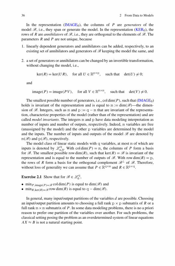
36 2 From Data to Models
In the representation (IMAGE0), the columns of P are generators of themodel B, i.e., they span or generate the model. In the representation (KER0), therows of R are annihilators of B, i.e., they are orthogonal to the elements of B. Theparameters R and P are not unique, because
1. linearly dependent generators and annihilators can be added, respectively, to anexisting set of annihilators and generators of B keeping the model the same, and
2. a set of generators or annihilators can be changed by an invertible transformation,without changing the model, i.e.,
ker(R)= ker(UR), for all U ∈Rp×p, such that det(U) �= 0;
and
image(P )= image(PV ), for all V ∈Rm×m, such that det(V ) �= 0.
The smallest possible number of generators, i.e., col dim(P ), such that (IMAGE0)holds is invariant of the representation and is equal to m := dim(B)—the dimen-sion of B. Integers, such as m and p := q− m that are invariant of the representa-tion, characterize properties of the model (rather than of the representation) and arecalled model invariants. The integers m and p have data modeling interpretation asnumber of inputs and number of outputs, respectively. Indeed, m variables are free(unassigned by the model) and the other p variables are determined by the modeland the inputs. The number of inputs and outputs of the model B are denoted bym(B) and p(B), respectively.
The model class of linear static models with q variables, at most m of which areinputs is denoted by L q
m,0. With col dim(P ) = m, the columns of P form a basisfor B. The smallest possible row dim(R), such that ker(R)=B is invariant of therepresentation and is equal to the number of outputs of B. With row dim(R) = p,the rows of R form a basis for the orthogonal complement B⊥ of B. Therefore,without loss of generality we can assume that P ∈R
q×m and R ∈Rp×q.
Exercise 2.1 Show that for B ∈L q0 ,
• minP,image(P )=B col dim(P ) is equal to dim(B) and• minR,ker(R)=B row dim(R) is equal to q− dim(B).
In general, many input/output partitions of the variables d are possible. Choosingan input/output partition amounts to choosing a full rank p× p submatrix of R or afull rank m×m submatrix of P . In some data modeling problems, there is no a priorireason to prefer one partition of the variables over another. For such problems, theclassical setting posing the problem as an overdetermined system of linear equationsAX ≈ B is not a natural starting point.

2.1 Linear Static Model Representations 37
Transition Among Input/Output, Kernel, and ImageRepresentations
The transition from one model representation to another gives insight into the prop-erties of the model. These analysis problems need to be solved before the more com-plicated modeling problems are considered. The latter can be viewed as synthesisproblems since the model is created or synthesized from data and prior knowledge.
If the parameters R, P , and (X,Π) describe the same system B, then they arerelated. We show the relations that the parameters must satisfy as well as code thatdoes the transition from one representation to another. Before we describe the transi-tion among the parameters, however, we need an efficient way to store and multiplyby permutation matrices and a tolerance for computing rank numerically.
Input/Output Partition of the Variables
In the input/output model representation Bi/o(X,Π), the partitioning of the vari-ables d ∈ R
q into inputs u ∈ Rm and outputs y ∈ R
p is specified by a permutationmatrix Π ,
d
Π−1=Π�
col(u, y),
Π
d =Π
[u
y
],
[u
y
]=Π�d.
In the software implementation, however, it is more convenient (as well as morememory and computation efficient) to specify the partitioning by a vector
π :=Π col(1, . . . ,q) ∈ {1, . . . ,q}q.Clearly, the vector π contains the same information as the matrix Π and one canreconstruct Π from π by permuting the rows of the identity matrix. (In the code iois the variable corresponding to the vector π and Pi is the variable correspondingto the matrix Π .)
37a 〈π →Π 37a〉≡ (38a)Pi = eye(length(io)); Pi = Pi(io,:);
Permuting the elements of a vector is done more efficiently by direct reordering ofthe elements, instead of a matrix-vector multiplication. If d is a variable correspond-ing to a vector d , then d(io) corresponds to the vector Πd .
The default value for Π is the identity matrix I , corresponding to first m variablesof d being inputs and the remaining p variables outputs, d = [ u
y
].
37b 〈default input/output partition 37b〉≡ (39 40a 42a)if ~exist(’io’) || isempty(io), io = 1:q; end
In case the inverse permutation Π−1 =Π� is needed, the corresponding “permuta-tion vector” is
π ′ =Π� col(1, . . . ,q) ∈ {1, . . . ,q}q.

38 2 From Data to Models
In the code inv_io is the variable corresponding to the vector π ′ and the transitionfrom the original variables d to the partitioned variables uy = [u; y] via io andinv_io is done by the following indexing operations:
dio_inv
uy,
io
d = uy(io), uy = d(io_inv).
38a 〈inverse permutation 38a〉≡ (42b)〈π →Π 37a〉, inv_io = (1:length(io)) * Pi;
Tolerance for Rank Computation
In the computation of an input/output representation from a given kernel or imagerepresentation of a model (as well as in the computation of the models’ complexity),we need to find the rank of a matrix. Numerically this is an ill-posed problem be-cause arbitrary small perturbations of the matrix’s elements may (generically will)change the rank. A solution to this problem is to replace rank with “numerical rank”defined as follows
num rank(A, ε) := number of singular values of A greater than ε, (num rank)
where ε ∈R+ is a user defined tolerance. Note that
num rank(A,0)= rank(A),
i.e., by taking the tolerance to be equal to zero, the numerical rank reduces to thetheoretical rank. A nonzero tolerance ε makes the numerical rank robust to pertur-bations of size (measured in the induced 2-norm) less than ε. Therefore, ε reflectsthe size of the expected errors in the matrix. The default tolerance is set to a smallvalue, which corresponds to numerical errors due to a double precision arithmetic.(In the code tol is the variable corresponding to ε.)
38b 〈default tolerance tol 38b〉≡ (41–43 76b)if ~exist(’tol’) || isempty(tol), tol = 1e-12; end
Note 2.2 The numerical rank definition (num rank) is the solution of an unstruc-tured rank minimization problem: find a matrix A of minimal rank, such that‖A− A‖2 < ε.
From Input/Output Representation to Kernel or Image Representations
Consider a linear static model B ∈L qm,0, defined by an input/output representation
Bi/o(X,Π). From y =X�u, we have[X� −I
]col(u, y)= 0

2.1 Linear Static Model Representations 39
or since d =Π[ u
y
],
[X� −I
]Π�
︸ ︷︷ ︸R
Π
[u
y
]
︸ ︷︷ ︸d
= 0.
Therefore, the matrix
R = [X� −I]Π� ((X,Π) →R)
is a parameter of a kernel representations of B, i.e.,
Bi/o(X,Π)= ker([
X� −I]Π�)=B.
Moreover, the representation is minimal because R is full row rank.Similarly, a minimal image representation is derived from the input/output rep-
resentation as follows. From y =X�u,[u
y
]=[
I
X�]
u,
so that, using d =Π[ u
y
],
d =Π
[u
y
]=Π
[I
X�]
u=: Pu.
Therefore, the matrix
P =Π
[I
X�]
((X,Π) → P )
is a parameter of an image representations of B, i.e.,
Bi/o(X,Π)= image
(Π
[I
X�])=B.
The representation is minimal because P is full column rank.Formulas ((X,Π) →R) and ((X,Π) → P ) give us a straight forward way of
transforming a given input/output representation to minimal kernel and minimalimage representations.
39 〈(X,Π) →R 39〉≡function r = xio2r(x, io)r = [x’, -eye(size(x, 2))]; q = size(r, 2);〈default input/output partition 37b〉, r = r(:, io);
Defines:xio2r, used in chunk 45a.

40 2 From Data to Models
40a 〈(X,Π) → P 40a〉≡function p = xio2p(x, io)p = [eye(size(x, 1)); x’]; q = size(p, 1);〈default input/output partition 37b〉, p = p(io, :);
Defines:xio2p, used in chunk 45a.
From Image to Minimal Kernel and from Kernel to Minimal ImageRepresentation
The relation
ker(R)= image(P )=B ∈L qm,0 =⇒ RP = 0 (R↔ P )
gives a link between the parameters P and R. In particular, a minimal image rep-resentation image(P ) = B can be obtained from a given kernel representationker(R) =B by computing a basis for the null space of R. Conversely, a minimalkernel representation ker(R)=B can be obtained from a given image representa-tion image(P )=B by computing a basis for the left null space of P .
40b 〈R → P 40b〉≡function p = r2p(r), p = null(r);
Defines:r2p, used in chunks 44 and 45a.
40c 〈P →R 40c〉≡function r = p2r(p), r = null(p’)’;
Defines:p2r, used in chunk 45a.
Converting an Image or Kernel Representation to a Minimal One
The kernel and image representations obtained from xio2r, xio2p, p2r, and r2pare minimal. In general, however, a given kernel or image representations can benon-minimal, i.e., R may have redundant rows and P may have redundant columns.The kernel representation, defined by R, is minimal if and only if R is full row rank.Similarly, the image representation, defined by P , is minimal if and only if P is fullcolumn rank.
The problems of converting kernel and image representations to minimal onesare equivalent to the problem of finding a full rank matrix that has the same kernelor image as a given matrix. A numerically reliable way to solve this problem is touse the singular value decomposition.
Consider a model B ∈L qm,0 with parameters R ∈ R
g×q and P ∈ Rq×g of, re-
spectively, kernel and image representations. Let
R =UΣV �

2.1 Linear Static Model Representations 41
be the singular value decomposition of R and let p be the rank of R. With thepartitioning,
V =: [V1 V2], where V1 ∈R
q×p,
we have
image(R�)= image(V1).
Therefore,
ker(R)= ker(V �1)
and V1 is full rank,
so that V �1 is a parameter of a minimal kernel representation of B.Similarly, let
P =UΣV�
be the singular value decomposition of P . With the partitioning,
U =: [U1 U2], where U1 ∈R
q×m,
we have
image(P )= image(U1).
Since U1 is full rank, it is a parameter of a minimal image representation of B.In the numerical implementation, the rank is replaced by the numerical rank with
respect to a user defined tolerance tol.
41 〈R →minimal R 41〉≡function r = minr(r, tol)[p, q] = size(r); 〈default tolerance tol 38b〉[u, s, v] = svd(r, ’econ’); pmin = sum(diag(s) > tol);if pmin < p, r = v(:, 1:pmin)’; end
Defines:minr, used in chunks 42b and 43c.
Exercise 2.3 Write a function minp that implements the transition P →minimal P .
From Kernel or Image to Input/Output Representation
The transformations from kernel to input/output and from image to input/outputrepresentations are closely related. They involve as a sub-problem the problem offinding input/output partitions of the variables in the model. Because of this, theyare more complicated than the inverse transformations, considered above.
Assume first that the input/output partition is given. This amounts to knowing thepermutation matrix Π ∈R
q×q in (I/O0).

42 2 From Data to Models
42a 〈(R,Π) →X 42a〉≡ 42b�function x = rio2x(r, io, tol)q = size(r, 2); 〈default input/output partition 37b〉, 〈default tolerance tol 38b〉
Defines:rio2x, used in chunks 43c and 45.
Consider given parameters R ∈ Rp×q of minimal kernel representation of a linear
static system B ∈L qm,0 and define the partitioning
RΠ =: [Ru Ry
], where Ry ∈R
p×p.
42b 〈(R,Π) →X 42a〉+≡ �42a 42c�r = minr(r, tol); p = size(r, 1); m = q - p;〈inverse permutation 38a〉, rpi = r(:, inv_io);ru = rpi(:, 1:m); ry = rpi(:, (m + 1):end);
Uses minr 41.
Similarly, for a parameter P ∈Rq×m of minimal image representation of B, de-
fine
Π�P =:[Pu
Py
], where Pu ∈R
m×m.
If Ry and Pu are non-singular, it follows from ((X,Π) →R) and ((X,Π) → P )that
X =−(R−1y Ru
)� ((R,Π) →X)
and
X = (PyP−1u
)� ((P,Π) →X)
is the parameter of the input/output representation Bi/o(X,Π) of B, i.e.,
ker( m p[
Ru Ry
]Π�
︸ ︷︷ ︸R
)=Bi/o
(−(R−1y Ru
)�,Π)
and
image
(
Π
[Pu
Py
]
︸ ︷︷ ︸P
mp
)
=Bi/o((
PyP−1u
)�,Π).
42c 〈(R,Π) →X 42a〉+≡ �42b[u, s, v] = svd(ry); s = diag(s);if s(end) < tol
warning(’Computation of X is ill conditioned.’);x = NaN;
elsex = -( v * diag(1 ./ s) * u’ * ru )’;
end

2.1 Linear Static Model Representations 43
Singularity of the blocks Ry and Pu implies that the input/output representation witha permutation matrix Π is not possible. In such cases, the function rio2x issues awarning message and returns NaN value for X.
The function r2io uses rio2x in order to find all possible input/output parti-tions for a model specified by a kernel representation.
43a 〈R →Π 43a〉≡ 43b�function IO = r2io(r, tol)q = size(r, 2); 〈default tolerance tol 38b〉
Defines:r2io, used in chunk 43d.
The search is exhaustive over all input/output partitionings of the variables (i.e., allchoices of m elements of the set of variable indices {1, . . . ,q}), so that the compu-tation is feasible only for a small number of variables (say less than 6).
43b 〈R →Π 43a〉+≡ �43a 43c�IO = perms(1:q); nio = size(IO, 1);
The parameter X for each candidate partition is computed. If the computation of X
is ill conditioned, the corresponding partition is not consistent with the model andis discarded.
43c 〈R →Π 43a〉+≡ �43bnot_possible = []; warning_state = warning(’off’);r = minr(r, tol);for i = 1:nio
x = rio2x(r, IO(i, :), tol);if isnan(x), not_possible = [not_possible, i]; end
endwarning(warning_state); IO(not_possible, :) = [];
Uses minr 41 and rio2x 42a.
Example 2.4 Consider the linear static model with three variables and one input
B = image
⎛
⎝
⎡
⎣100
⎤
⎦
⎞
⎠= ker
([0 1 00 0 1
]).
Clearly, this model has only two input/output partitions:
u=w1, y =[w2w3
]and u=w1, y =
[w3w2
].
Indeed, the function r2io
43d 〈Test r2io 43d〉≡r2io([0 0 1; 0 1 0])
Uses r2io 43a.

44 2 From Data to Models
Fig. 2.1 Relations andfunctions for the transitionsamong linear static modelparameters
correctly computes the input output partitionings from the parameter R in a kernelrepresentation of the modelans =
1 2 31 3 2
Exercise 2.5 Write functions pio2x and p2io that implement the transitions
(P,Π) →X and P →Π.
Exercise 2.6 Explain how to check that two models, specified by kernel or imagerepresentation, are equivalent.
Summary of Transitions among Representations
Figure 2.1 summarizes the links among the parameters R, P , and (X,Π) of a linearstatic model B and the functions that implement the transitions.
Numerical Example
In order to test the functions for transition among the kernel, image, and input/outputmodel representations, we choose, a random linear static model, specified by a ker-nel representation,
44 〈Test model transitions 44〉≡ 45a�m = 2; p = 3; R = rand(p, m + p); P = r2p(R);
Uses r2p 40b.

2.2 Linear Time-Invariant Model Representations 45
and traverse the diagram in Fig. 2.1 clock-wise and anti clock-wise45a 〈Test model transitions 44〉+≡ �44 45b�
R_ = xio2r(pio2x(r2p(R))); P_ = xio2p(rio2x(p2r(P)));
Uses p2r 40c, r2p 40b, rio2x 42a, xio2p 40a, and xio2r 39.
As a verification of the software, we check that after traversing the loop, equivalentmodels are obtained.
45b 〈Test model transitions 44〉+≡ �45anorm(rio2x(R) - rio2x(R_)), norm(pio2x(P) - pio2x(P_))
Uses rio2x 42a.
The answers are around the machine precision, which confirms that the models arethe same.
Linear Static Model Complexity
A linear static model is a finite dimensional subspace. The dimension m of the sub-space is equal to the number of inputs and is invariant of the model representation.The integer constant m quantifies the model complexity: the model is more complexwhen it has more inputs. The rationale for this definition of model complexity isthat inputs are “unexplained” variables by the model, so the more inputs the modelhas, the less it “explains” the modeled phenomenon. In data modeling the aim is toobtain low-complexity models, a principle generally referred to as Occam’s razor.
Note 2.7 (Computing the model complexity is a rank estimation problem) Comput-ing the model complexity, implicitly specified by (exact) data, or by a non-minimalkernel or image representation is a rank computation problem; see Sect. 2.3 and thefunction minr.
2.2 Linear Time-Invariant Model Representations
An observation dj of a static model is a vector of variables. In the dynamic case,the observations depend on time, so that apart from the multivariable aspect, there isalso a time evaluation aspect. In the dynamic case, an observation is referred to as atrajectory, i.e., it is a vector valued function of a scalar argument. The time variabletakes its values in the set of integers Z (discrete-time model) or in the set of realnumbers R (continuous-time model). We denote the time axis by T .
A dynamic model B with q variables is a subset of the trajectory space(Rq)T —the set of all functions from the time axis T to the variablespace R
q.

46 2 From Data to Models
In this book, we consider the special class of finite dimensional linear time-invariant dynamical models. By definition, a model B is linear if it is a subspace ofthe data space (Rq)T . In order to define the time-invariance property, we introducethe shift operator σ τ . Acting on a signal w, σ τ produces a signal σ τw, which is thebackwards shifted version of w by τ time units, i.e.,
(σ τw
)(t) :=w(t + τ), for all t ∈T .
Acting on a set of trajectories, σ τ shifts all trajectories in the set, i.e.,
σ τB := {σ τw |w ∈B}.
A model B is shift-invariant if it is invariant under any shift in time, i.e.,
σ τB =B, for all τ ∈T .
The model B is finite dimensional if it is a closed subset (in the topology of point-wise convergence). Finite dimensionality is equivalent to the property that at anytime t the future behavior of the model is deterministically independent of the pastbehavior, given a finite dimensional vector, called a state of the model. Intuitively,the state is the information (or memory) of the past that is needed in order to predictthe future. The smallest state dimension is an invariant of the system, called theorder. We denote the set of finite dimensional linear time-invariant models with qvariables and order at most n by L q,n and the order of B by n(B).
A finite dimensional linear time-invariant model B ∈L q,n admits a representa-tion by a difference or differential equation
R0w+R1λw+ · · · +Rlλlw = (R0 +R1λ+ · · · +Rlλ
l︸ ︷︷ ︸
R(λ)
)w
=R(λ)w = 0,
(DE)
where λ is the unit shift operator σ in the discrete-time case and the differentialoperator d
dtin the continuous-time case. Therefore, the model B is the kernel
B := ker(R(λ)
)= {w | (DE) holds}, (KER)
of the difference or differential operator R(λ). The smallest degree l of a polyno-mial matrix
R(z) :=R0 +R1z+ · · · +Rlzl ∈R
g×q[z],in a kernel representation (KER) of B, is invariant of the representation and is calledthe lag l(B) of B.
The order of the system is the total degree of the polynomial matrix R in a kernelrepresentation of the system. Therefore, we have the following link between theorder and the lag of a linear time-invariant model:
n(B)≤ p(B)l(B).

2.2 Linear Time-Invariant Model Representations 47
As in the static case, the smallest possible number of rows g of the polyno-mial matrix R in a kernel representation (KER) of a finite dimensional linear time-invariant system B is the invariant p(B)—number of outputs of B. Finding aninput/output partitioning for a model specified by a kernel representation amountsto selection of a non-singular p×p submatrix of R. The resulting input/output rep-resentation is:
B =Bi/o(P,Q,Π) := ker(Π[Q(λ) P (λ)
]), (I/O)
with parameters the polynomial matrices
Q ∈Rp×m[z] and P ∈R
p×p[z], such that det(P ) �= 0,
and the permutation matrix Π .In general, the representation (I/O) involves higher order shifts or derivatives.
A first order representation
B =Bi/s/o(A,B,C,D,Π) := {w =Π col(u, y) | there is x, such that
λx =Ax +Bu and y = Cx +Du}, (I/S/O)
with an auxiliary variable x, however, is always possible. The representation (I/S/O)displays not only the input/output structure of the model but also its state structureand is referred to as an input/state/output representation of the model. The parame-ters of an input/state/output representation are the matrices
A ∈Rn×n, B ∈R
n×m, C ∈Rp×n, D ∈R
p×m,
and a permutation matrix Π . The parameters are nonunique due to
• nonuniqueness in the choice of the input/output partition,• existence of redundant states (non-minimality of the representation), and• change of state space basis
Bi/s/o(A,B,C,D)=Bi/s/o(T −1AT,T −1B,CT ,D
),
for any non-singular matrix T ∈Rn×n. (CB)
An input/state/output representation Bi/s/o(A,B,C,D) is called minimal when thestate dimension n is as small as possible. The minimal state dimension is an invari-ant of the system and is equal to the order n(B) of the system.
A system B is autonomous if for any trajectory w ∈B the “past”
w− :=(. . . ,w(−2),w(−1)
)
of w completely determines its “future”
w+ :=(w(0),w(1), . . .
).

48 2 From Data to Models
Table 2.1 Summary of model B ⊂ (Rq)T properties
Property Definition
linearity w,v ∈B =⇒ αw+ βv ∈B, for all α,β ∈R
time-invariance στ B =B, for all τ ∈T
finite dimensionality B is a closed set; equivalently n(B) <∞autonomy the past of any trajectory completely determines its future;
equivalently m(B)= 0
controllability the past of any trajectory can be concatenated to the future of any
other trajectory by a third trajectory if a transition period is allowed
It can be shown that a system B is autonomous if and only if it has no inputs. Anautonomous finite dimensional linear time-invariant system is parametrized by thepair of matrices A and C via the state space representation
Bi/s/o(A,C) := {w = y | there is x, such that σx =Ax and y = Cx}.
The dimension dim(B) of an autonomous linear model B is equal to the or-der n(B).
In a way the opposite of an autonomous model is a controllable system. Themodel B is controllable if for any trajectories wp and wf of B, there is τ > 0 and athird trajectory w ∈B, which coincides with wp in the past, i.e., w(t)=wp(t), forall t < 0, and coincides with wf in the future, i.e., w(t)= wf(t), for all t ≥ τ . Thesubset of controllable systems of the set of linear time-invariant systems L q is de-noted by L q
ctrb. A summary of properties of a dynamical system is given in Table 2.1.Apart from the kernel, input/output, and input/state/output representation, a con-
trollable finite dimensional linear time-invariant model admits the following repre-sentations:
• image representation
B = image(P(λ)
) := {w |w = P(λ)�, for some �}, (IMAGE)
with parameter the polynomial matrix P(z) ∈Rq×g[z],
• convolution representation
B =Bi/o(H,Π) := {w =Π col(u, y) | y =H � u}, (CONV)
where � is the convolution operator
y(t)= (H � u)(t) :=∞∑
τ=0
H(τ)u(t − τ), in discrete-time, or
y(t)= (H � u)(t) :=∫ ∞
0H(τ)u(t − τ)dτ, in continuous-time,
with parameters the signal H :T →Rp×m and a permutation matrix Π ; and

2.2 Linear Time-Invariant Model Representations 49
Fig. 2.2 Data, input/output model representations, and links among them
• transfer function,
B =Bi/o(H,Π) := {w =Π col(u, y) |F (y)=H(z)F (u)}, (TF)
where F is the Z-transform in discrete-time and the Laplace transform incontinuous-time, with parameters the rational matrix H ∈ R
p×m(s) (the transferfunction) and a permutation matrix Π .
Transitions among the parameters H , H(z), and (A,B,C,D) are classical prob-lems, see Fig. 2.2. Next, we review the transition from impulse response H to pa-rameters (A,B,C,D) of an input/state/output representation, which plays an im-portant role in deriving methods for Hankel structured low rank approximation.
System Realization
The problem of passing from a convolution representation to an input/state/outputrepresentation is called (impulse response) realization.
Definition 2.8 (Realization) A linear time-invariant system B with m inputs and poutputs and an input/output partition, specified by a permutation matrix Π , is a real-ization of (or realizes) an impulse response H :T →R
p×m if B has a convolution

50 2 From Data to Models
representation B =Bi/o(H,Π). A realization B of H is minimal if its order n(B)
is the smallest over all realization of H .
In what follows, we fix the input/output partition Π to the default one
w = col(u, y)
and use the notation
H := [h1 · · · hm]
and Im :=[e1 · · · em
].
An equivalent definition of impulse response realization that makes explicit thelink of the realization problem to data modeling is the following one.
Definition 2.9 (Realization, as a data modeling problem) The system B realizes H
if the set of input/output trajectories (ei, hi), for i = 1, . . . ,m are impulse responsesof B, i.e.,
(eiδ,0∧ hi) ∈B, for i = 1, . . . ,m,
where δ is the delta function and ∧ is the concatenation map (at time 0)
w =wp ∧wf, w(t) :={
wp(t), if t < 0
wf(t), if t ≥ 0
Note 2.10 (Discrete-time vs. continuous-time system realization) There are somedifferences between the discrete and continuous-time realization theory. Next, weconsider the discrete-time case. It turns out, however, that the discrete-time algo-rithms can be used for realization of continuous-time systems by applying them onthe sequence of the Markov parameter (H(0), d
d tH(0), . . .) of the system.
The sequence
H = (H(0),H(1),H(2), . . . ,H(t), . . .), where H(t) ∈R
p×m
is a one sided infinite matrix-values time series. Acting on H , the shift operator σ ,removes the first sample, i.e.,
σH = (H(1),H(2), . . . ,H(t), . . .).
A sequence H might not be realizable by a finite dimensional linear time-invariant system, but if it is realizable, a minimal realization is unique.
Theorem 2.11 (Test for realizability) The sequence H : Z+ →Rp×m is realizable
by a finite dimensional linear time-invariant system with m inputs if and only if thetwo-sided infinite Hankel matrix H (σH) has a finite rank n. Moreover, the orderof a minimal realization is equal to n, and there is a unique system B in L q,n
m thatrealizes H .

2.2 Linear Time-Invariant Model Representations 51
Proof (=⇒) Let H be realizable by a system B ∈ L q,nm with a minimal in-
put/state/output representation B =Bi/s/o(A,B,C,D). Then
H(0)=D and H(t)= CAt−1B, for t > 0.
The (i, j) block element of the Hankel matrix H (σH) is
H(i + j − 1)= CAi+j−2B = CAi−1Aj−1B.
Let
Ot (A,C) := col(C,CA, . . . ,CAt−1) (O)
be the extended observability matrix of the pair (A,C) and
Ct (A,B) := [B AB · · · At−1B]
(C )
be the extended controllability matrix of the pair (A,B). With O(A,C) andC (A,B) being the infinite observability and controllability matrices, we have
H (σH)=O(A,C)C (A,B) (OC )
Since the representation Bi/s/o(A,B,C,D) is assumed to be minimal, C (A,B) isfull row rank and O(A,C) is full column rank. Therefore, (OC ) is a rank revealingfactorization of H (σH) and
rank(H (σH)
)= n(B).
(⇐=) In this direction, the proof is constructive and results in an algorithm forcomputation of the minimal realization of H in L q,n
m , where n= rank(H (σH)).A realization algorithm is presented in Sect. 3.1. �
Theorem 2.11 shows that
rank(Hi,j (σH)
)= n(B), for pi ≥ n(B) and mj ≥ n(B).
This suggests a method to find the order n(B) of the minimal realization of H :compute the rank of the finite Hankel matrix Hi,j (σH), where nmax :=min(pi,mj)
is an upper bound of the order. Algorithms for computing the order and parametersof the minimal realization are presented in Chap. 3.1.
Linear Time-Invariant Model Complexity
Associate with a linear time-invariant dynamical system B, we have defined thefollowing system invariants:
m(B) number of inputs, n(B) order,
p(B) number of outputs and l(B) lag.

52 2 From Data to Models
The complexity of a linear static model B is the number of inputs m(B) of Bor, equivalently, the dimension dim(B) of B. Except for the class of autonomoussystems, however, the dimension of a dynamical model is infinite. We define therestriction B|[1,T ] of B to the interval [1, T ],
B|[1,T ] :={w ∈R
T | there exist wp and wf, such that (wp,w,wf) ∈B}.
(B|[1,T ])For a linear time-invariant model B and for T > n(B),
dim(B|[1,T ])= m(B)T + n(B)≤ m(B)T + l(B)p(B), (dim B)
which shows that the pairs of natural numbers
(m(B),n(B)
)and
(m(B),l(B)
)
characterize the model’s complexity. The elements of the model class L qm,l are lin-
ear time-invariant systems of complexity bounded by the pair (m,l) and, similarly,the elements of the model class L q,n
m are linear time-invariant systems of complex-ity bounded by the pair (m,n). A static model is a special case of a dynamic modelwhen the lag (or the order) is zero. This is reflected in the notation L q,n
m,l : the linearstatic model class Lm,0 corresponds to the linear time-invariant model class Lm,l
with l= 0.Note that in the autonomous case, i.e., with m(B)= 0, dim(B)= n. The dimen-
sion of the system corresponds to the number of degrees of freedom in selectinga trajectory. In the case of an autonomous system, the trajectory depends only onthe initial condition (an n(B) dimensional vector). In the presence of inputs, thenumber of degrees of freedom due to the initial condition is increased on each timestep by the number of inputs, due to the free variables. Asymptotically as T →∞,the term mT in (dim B) dominates the term n. Therefore, in comparing linear time-invariant system’s complexities, by convention, a system with more inputs is morecomplex than a system with less inputs, irrespective of their state dimensions.
2.3 Exact and Approximate Data Modeling
General Setting for Data Modeling
In order to treat static, dynamic, linear, and nonlinear modeling problems with uni-fied terminology and notation, we need an abstract setting that is general enough toaccommodate all envisaged applications. Such a setting is described in this section.
The data D and a model B for the data are subsets of a universal set U of pos-sible observations. In static modeling problems, U is a real q-dimensional vectorspace R
q, i.e., the observations are real valued vectors. In dynamic modeling prob-lems, U is a function space (Rq)T , with T being Z in the discrete-time case and R
in the continuous-time case.

2.3 Exact and Approximate Data Modeling 53
Note 2.12 (Categorical data and finite automata) In modeling problems with cate-gorical data and finite automata, the universal set U is discrete and may be finite.
We consider data sets D consisting of a finite number of observations
D = {wd,1, . . . ,wd,N } ⊂U .
In discrete-time dynamic modeling problems, the wd,j ’s are trajectories, i.e.,
wd,j =(wd,j (1), . . . ,wd,j (Tj )
), with wd,j (t) ∈R
q for all t .
In dynamic problems, the data D often consists of a single trajectory wd,1, in whichcase the subscript index 1 is skipped and D is identified with wd. In static modelingproblems, an observation wd,j is a vector and the alternative notation dj = wd,j isused in order to emphasize the fact that the observations do not depend on time.
Note 2.13 (Given data vs. general trajectory) In order to distinguish a general tra-jectory w of the system from the given data wd (a specific trajectory) we use thesubscript “d” in the notation of the given data.
A model class M is a set of sets of U , i.e., M is an element of the power set 2U
of U . We consider the generic model classes of
• linear static models L0,• linear time-invariant models L , and• polynomial static models P (see Chap. 6).
In some cases, however, subclasses of the generic classes above are of interest. Forexamples, the controllable and finite impulse response model subclasses of the classof linear time-invariant models, and the ellipsoids subclass of the class of secondorder polynomial models (conic sections).
The complexity c of a model B is a vector of positive integers
c(B) :=
⎧⎪⎨
⎪⎩
m(B)= dim(B), if B ∈L0,
(m(B),l(B)) or (m(B),n(B)), if B ∈L ,
(m(B),deg(R)), where B = ker(R), if B ∈P.
(c(B))
Complexities are compared in this book by the lexicographic ordering, i.e., twocomplexities are compared by comparing their corresponding elements in the in-creasing order of the indices. The first time an index is larger, the correspondingcomplexity is declared larger. For linear time-invariant dynamic models, this con-vention and the ordering of the elements in c(B) imply that a model with moreinputs is always more complex than a model with less inputs irrespective of theirorders.
The complexity c of a model class M is the largest complexity of a model inthe model class. Of interest is the restriction of the generic model classes M tosubclasses Mcmax of models with bounded complexity, e.g., L q
m,lmax, with m< q.

54 2 From Data to Models
Exact Data Modeling
A model B is an exact model for the data D if D ⊂B. Otherwise, it is an approx-imate model. An exact model for the data may not exist in a model class Mcmax
of bounded complexity. This is generically the case when the data are noisy andthe data set D is large enough (relative to the model complexity). A practical datamodeling problem must involve approximation. Our starting point, however, is thesimpler problem of exact data modeling.
Problem 2.14 (Exact data modeling) Given data D ⊂ U and a model classMcmax ∈ 2U , find a model B in Mcmax that contains the data and has minimal(in the lexicographic ordering) complexity or assert that such a model does not ex-ist, i.e.,
minimize over B ∈Mcmax c(B) subject to D ⊂B (EM)
The question occurs:
(Existence of exact model) Under what conditions on the data D and themodel class Mcmax does a solution to problem (EM) exist?
If a solution exists, it is unique. This unique solution is called the most pow-erful unfalsified model for the data D in the model class Mcmax and is denotedby Bmpum(D). (The model class Mcmax is not a part of the notation Bmpum(D) andis understood from the context.)
Suppose that the data D are generated by a model B0 in the model class Mcmax ,i.e.,
D ⊂B0 ∈Mcmax .
Then, the exact modeling problem has a solution in the model class Mcmax , however,the solution Bmpum(D) may not be the data generating model B0. The questionoccurs:
(Identifiability) Under what conditions on the data D , the data generat-ing model B0, and the model class Mcmax , the most powerful unfalsifiedmodel Bmpum(D) in Mcmax coincides with the data generating model B0?
Example 2.15 (Exact data fitting by a linear static model) Existence of a linear staticmodel B of bounded complexity m for the data D is equivalent to rank deficiencyof the matrix
Φ(D) := [d1 · · · dN
] ∈Rq×N,

2.3 Exact and Approximate Data Modeling 55
composed of the data. (Show this.) Moreover, the rank of the matrix Φ(D) is equalto the minimal dimension of an exact model for D
existence of B ∈L qm,0, such that D ⊂ B ⇐⇒ rank
(Φ(D)
)≤ m. (∗)
The exact model
B = image(Φ(D)
)(∗∗)
of minimal dimension
c(B)= rank(Φ(D)
)
always exists and is unique.The equivalence (∗) between data modeling and the concept of rank is the basis
for application of linear algebra and matrix computations to linear data modeling.Indeed, (∗∗) provides an algorithm for exact linear static data modeling. As shownnext, exact data modeling has also direct relevance to approximate data modeling.
Approximate Data Modeling
When an exact model does not exist in the considered model class, an approximatemodel that is in some sense “close” to the data is aimed at instead. Closeness ismeasured by a suitably defined criterion. This leads to the following approximatedata modeling problem.
Problem 2.16 (Approximate data modeling) Given data D ⊂ U , a model classMcmax ∈ 2U , and a measure f (D,B) for the lack of fit of the data D by a model B,find a model B in the model class Mcmax that minimizes the lack of fit, i.e.,
minimize over B ∈Mcmax f (D,B). (AM)
Since an observation w is a point in and the model B is a subset of the dataspace U , it is natural to measure the lack of fit between w and B by the geometricdistance
dist(w,B) := minw∈B
∥∥w− w∥∥
2. (dist(w,B))
The auxiliary variable w is the best approximation of w in B. Geometrically, it isthe orthogonal projection of w on B.
For the set of observations D , we define the distance from D to B as
dist(D,B) := minw1,...,wN∈B
√√√√√N∑
j=1
∥∥wd,j − wj
∥∥22. (dist)

56 2 From Data to Models
The set of points
D = {w1, . . . , wN
}
in the definition of (dist) is an approximation of the data D in the model B.Note that problem (dist) is separable, i.e., it decouples into N independent prob-lems (dist(w,B)).
Algorithms for computing the geometric distance are discussed in Sect. 3.2, inthe case of linear models, and in Chap. 6, in the case of polynomial models.
Note 2.17 (Invariance of (dist) to rigid transformation) The geometric distancedist(D,B) is invariant to a rigid transformation, i.e., translation, rotation, and re-flection of the data points and the model.
An alternative distance measure, called algebraic distance, is based on a kernelrepresentation B = ker(R) of the model B. Since R is a mapping from U to R
g ,such that
w ∈B ⇐⇒ R(w)= 0,
we have∥∥R(w)
∥∥F > 0 ⇐⇒ w /∈B.
The algebraic “distance” measures the lack of fit between w and B by the “size”‖R(w)‖F of the residual R(w). For a data set D , we define
dist′(D,B) :=
√√√√√N∑
j=1
∥∥R(wd,j )
∥∥2
F. (dist′)
The algebraic distance depends on the choice of the parameter R in a kernel rep-resentation of the model, while the geometric distance is representation invariant. Inaddition, the algebraic distance is not invariant to a rigid transformation. However,a modification of the algebraic distance that is invariant to a rigid transformation ispresented in Sect. 6.3.
Example 2.18 (Geometric distance for linear and quadratic models) The two plotsin Fig. 2.3 illustrate the geometric distance (dist) from a set of eight data points
D = {di = (xi, yi) | i = 1, . . . ,8}
in the plane to, respectively, linear B1 and quadratic B2 models. As its name sug-gests, dist(D,B) has geometric interpretation—in order to compute the geometricdistance, we project the data points on the models. This is a simple task (linear leastsquares problem) for linear models but a nontrivial task (nonconvex optimizationproblem) for nonlinear models. In contrast, the algebraic “distance” (not visualizedin the figure) has no simple geometrical interpretation but is easy to compute forlinear and nonlinear models alike.

2.3 Exact and Approximate Data Modeling 57
Fig. 2.3 Geometric distance from eight data points to a linear (left) and quadratic (right) models
Note 2.19 (Approximate modeling in the case of exact data) If an exact model Bexists in the model class Mcmax , then B is a global optimum point of the approxi-mate modeling problem (AM) (irrespective of the approximation criterion f beingused). Indeed,
D ⊂B ⇐⇒ dist(D,B)= dist′(D,B)= 0.
An optimal approximate model, i.e., a solution of (AM), however, need not beunique. In contrast, the most powerful unfalsified model is unique. This is due tothe fact that (AM) imposes an upper bound but does not minimize the model com-plexity, while (EM) minimizes the model complexity. As a result, when
c(Bmpum(D)
)< cmax,
(AM) has a nonunique solution. In the next section, we present a more generalapproximate data modeling problem formulation that minimizes simultaneously thecomplexity as well as the fitting error.
The terminology “geometric” and “algebraic” distance comes from the computervision application of the methods for fitting curves and surfaces to data. In the sys-tem identification community, the geometric fitting method is related to the misfitapproach and the algebraic fitting criterion is related to the latency approach. Misfitand latency computation are data smoothing operations. For linear time-invariantsystems, the misfit and latency can be computed efficiently by Riccati type recur-sions. In the statistics literature, the geometric fitting is related to errors-in-variableestimation and the algebraic fitting is related to classical regression estimation, seeTable 2.2.
Example 2.20 (Algebraic fit and errors-in-variables modeling) From a statisticalpoint of view, the approximate data modeling problem (AM) with the geometricfitting criterion (dist) yields a maximum likelihood estimator for the true model B0in the errors-in-variables setup
wd,j =w0,j + wj , (EIV)

58 2 From Data to Models
Table 2.2 Correspondence among terms for data fitting criteria in different fields
Computer vision System identification Statistics Mathematics
geometric fitting misfit errors-in-variables implicit function
algebraic fitting latency regression function
where
D0 := {w0,1, . . . ,w0,N } ⊂B0
is the true data and
D := {w1, . . . , wN
}
is the measurement noise, which is assumed to be a set of independent, zero mean,Gaussian random vectors, with covariance matrix σ 2I .
Example 2.21 (Algebraic fit by a linear model and regression) A linear modelclass, defined by the input/output representation Bi/o(Θ) and algebraic fitting crite-rion (dist′), where
w := col(u, y) and R(w) :=Θ�u− y
lead to the ordinary linear least squares problem
minimize over Θ ∈Rm×p ∥∥Θ�Φ(ud)−Φ(yd)
∥∥F. (LS)
The statistical setting for the least squares approximation problem (LS) is the clas-sical regression model
R(wd,j )= ej , (REG)
where e1, . . . , eN are zero mean independent and identically distributed randomvariables. Gauss–Markov’s theorem states that the least squares approximate so-lution is the best linear unbiased estimator for the regression model (REG).
Complexity–Accuracy Trade-off
Data modeling is a mapping from a given data set D , to a model B in a given modelclass M :
data set D ⊂Udata modeling problem−−−−−−−−−−−−−→ model B ∈M ∈ 2U .
A data modeling problem is defined by specifying the model class M and one ormore modeling criteria. Basic criteria in any data modeling problem are:

2.3 Exact and Approximate Data Modeling 59
• “simple” model, measured by the model complexity c(B), and• “good” fit of the data by the model, measured by (vector) cost function F(D,B).
Small complexity c(B) and small fitting error F(D,B), however, are contradictingobjectives, so that a core issue throughout data modeling is the complexity–accuracytrade-off. A generic data modeling problem is:
Given a data set D ∈U and a measure F for the fitting error, solve the multi-objective optimization problem:
minimize over B ∈M
[c(B)
F (D,B)
]. (DM)
Next we consider the special cases of linear static models and linear time-invariant dynamic models with F(D,B) being dist(D,B) or dist′(D,B). Themodel class assumption implies that dim(B) is a complexity measure in both staticand dynamic cases.
Two Possible Scalarizations: Low Rank Approximation and RankMinimization
The data set D , can be parametrized by a real vector p ∈Rnp . (Think of the vector p
as a representation of the data in the computer memory.) For a linear model B andexact data D , there is a relation between the model complexity and the rank of adata matrix S (p):
c(Bmpum(D)
)= rank(S (p)
). (∗)
The mapping
S :Rnp →Rm×n
from the data parameter vector p to the data matrix S (p) depends on the applica-tion. For example, S (p) = Φ(D) is unstructured in the case of linear static mod-eling (see Example 2.15) and S (p) =H (wd) is Hankel structured in the case ofautonomous linear time-invariant dynamic model identification,
Let p be the parameter vector for the data D and p be the parameter vector forthe data approximation D . The geometric distance dist(D,B) can be expressed interms of the parameter vectors p and p as
minimize over p ‖p− p‖2 subject to D ⊂B.
Moreover, the norm in the parameter space Rnp can be chosen as weighted 1-, 2-,
and ∞-(semi)norms:

60 2 From Data to Models
‖p‖w,1 :=∥∥w� p
∥∥1 :=
np∑
i=1
∣∣wipi
∣∣,
‖p‖w,2 :=∥∥w� p
∥∥2 :=
√√√√np∑
i=1
(wip
)2,
‖p‖w,∞ :=∥∥w� p
∥∥∞ := maxi=1,...,np
∣∣wipi
∣∣,
(‖ · ‖w)
where w is a vector with nonnegative elements, specifying the weights, and� is theelement-wise (Hadamard) product.
Using the data parametrization (∗) and one of the distance measures (‖ · ‖w),the data modeling problem (DM) becomes the biobjective matrix approximationproblem:
minimize over p
[rank(S (p))
‖p− p‖]
. (DM’)
Two possible ways to scalarize the biobjective problem (DM’) are:
1. Misfit minimization subject to a bound r on the model complexity
minimize over p∥∥p− p
∥∥ subject to rank(S (p)
)≤ r. (SLRA)
2. Model complexity minimization subject to a bound ε on the fitting error
minimize over p rank(S (p)
)subject to
∥∥p− p∥∥≤ ε. (RM)
Problem (SLRA) is a structured low rank approximation problem and (RM) is arank minimization problem.
By varying the parameters r and ε from zero to infinity, both problems sweepthe trade-off curve (set of Pareto optimal solutions) of (DM’). Note, however, that r
ranges over the natural numbers and only small values are of practical interest. Inaddition, in applications often a “suitable” value for r can be chosen a priori or iseven a part of the problem specification. In contrast, ε is a positive real numberand is data dependent, so that a “suitable” value is not readily available. These con-siderations, suggest that the structured low rank approximation problem is a moreconvenient scalarization of (DM’) for solving practical data modeling problems.
Convex relaxation algorithms for solving (DM’) are presented in Sect. 3.3.
2.4 Unstructured Low Rank Approximation
Linear static data modeling leads to unstructured low rank approximation. Viceverse, unstructured low rank approximation problems can be given the interpreta-tion (or motivation) of linear static data modeling problems. As argued in Sect. 1.1,these are equivalent problems. The data modeling view of the problem makes link

2.4 Unstructured Low Rank Approximation 61
to applications. The low rank approximation view of the problem makes link tocomputational algorithms for solving the problem.
Problem 2.22 (Unstructured low rank approximation) Given a matrix D ∈ Rq×N ,
with q≤N , a matrix norm ‖ · ‖, and an integer m, 0 < m< q, find a matrix
D∗ := arg minD
∥∥D − D∥∥ subject to rank(D)≤ m. (LRA)
The matrix D∗ is an optimal rank-m (or less) approximation of D with respect tothe given norm ‖ · ‖.
The special case of (LRA) with ‖ · ‖ being the weighted 2-norm
‖�D‖W :=√
vec�(�D)W vec(�D), for all �D (‖ · ‖W )
where W ∈ RqN×qN is a positive definite matrix, is called weighted low rank ap-
proximation problem. In turn, special cases of the weighted low rank approximationproblem are obtained when the weight matrix W has diagonal, block diagonal, orsome other structure.
• Element-wise weighting:
W = diag(w1, . . . ,wqN), where wi > 0, for i = 1, . . . ,qN.
• Column-wise weighting:
W = diag(W1, . . . ,WN), where Wj ∈Rq×q, Wj > 0, for j = 1, . . . ,N.
• Column-wise weighting with equal weight matrix for all columns:
W = diag(Wl, . . . ,Wl), where Wl ∈Rq×q, Wl > 0.
• Row-wise weighting:
�W = diag(W1, . . . ,Wq), where Wi ∈RN×N, Wi > 0, for i = 1, . . . ,q,
and �W is a matrix, such that
‖�D‖W = ∥∥�D�∥∥�W, for all �D.
• Row-wise weighting with equal weight matrix for all rows:
�W = diag(Wr, . . . ,Wr︸ ︷︷ ︸q
), where Wr ∈RN×N, Wr > 0.
Figure 2.4 shows the hierarchy of weighted low rank approximation problems, ac-cording to the structure of the weight matrix W . Exploiting the structure of theweight matrix allows more efficient solution of the corresponding weighted low rankapproximation problems compared to the general problem with unstructured W .

62 2 From Data to Models
As shown in the next section left/right weighting with equal matrix forall rows/columns corresponds to the approximation criteria ‖√Wl�D‖F and‖�D
√Wr‖F. The approximation problem with criterion ‖√Wl�D
√Wr‖F is called
two-sided weighted and is also known as the generalized low rank approximationproblem. This latter problem allows analytic solution in terms of the singular valuedecomposition of the data matrix.
Special Cases with Known Analytic Solutions
An extreme special case of the weighted low rank approximation problem is the“unweighted” case, i.e., weight matrix a multiple of the identity W = v−1I , forsome v > 0. Then, ‖ · ‖W is proportional to the Frobenius norm ‖ · ‖F and the lowrank approximation problem has an analytic solution in terms of the singular valuedecomposition of D. The results is known as the Eckart–Young–Mirsky theorem orthe matrix approximation lemma. In view of its importance, we refer to this case asthe basic low rank approximation problem.
Theorem 2.23 (Eckart–Young–Mirsky) Let
D =UΣV �
be the singular value decomposition of D and partition U , Σ =: diag(σ1, . . . , σq),and V as follows:
U =:m q− m[U1 U2
]q , Σ =:
m q− m[Σ1 00 Σ2
]m
q− mand V =:
m q− m[V1 V2
]N .
Then the rank-m matrix, obtained from the truncated singular value decomposition
D∗ =U1Σ1V�1 ,
is such that
‖D − D∗‖F = minrank(D)≤m
‖D − D‖F =√
σ 2m+1 + · · · + σ 2
q .
The minimizer D∗ is unique if and only if σm+1 �= σm.
The proof is given in Appendix B.
Note 2.24 (Unitarily invariant norms) Theorem 2.23 holds for any norm ‖ · ‖ that isinvariant under orthogonal transformations, i.e., satisfying the relation
‖U�DV ‖ = ‖�D‖, for any �D and for any orthogonal matrices U and V .

2.4 Unstructured Low Rank Approximation 63
Fig. 2.4 Hierarchy of weighted low rank approximation problems according to the structure of theweight matrix W . On the left side are weighted low rank approximation problems with row-wiseweighting and on the right side are weighted low rank approximation problems with column-wiseweighting. The generality of the problem reduces from top to bottom
Note 2.25 (Approximation in the spectral norm) For a matrix �D, let ‖�D‖2 bethe spectral (2-norm induced) matrix norm
‖�D‖2 = σmax(�D).

64 2 From Data to Models
Then
minrank(D)=m
∥∥D− D∥∥
2 = σm+1,
i.e., the optimal rank-m spectral norm approximation error is equal to the first ne-glected singular value. The truncated singular value decomposition yields an opti-mal approximation with respect to the spectral norm, however, in this case a mini-mizer is not unique even when the singular values σm and σm+1 are different.
As defined, the low rank approximation problem aims at a matrix D that is asolution to the optimization problem (LRA). In data modeling problems, however,of primary interest is the optimal model, i.e., the most powerful unfalsified modelfor D∗. Theorem 2.23 gives the optimal approximating matrix D∗ in terms of thesingular value decomposition of the data matrix D. Minimal parameters of kerneland image representations of the corresponding optimal model are directly availablefrom the factors of the singular value decomposition of D.
Corollary 2.26 An optimal in the Frobenius norm approximate model for thedata D in the model class Lm,0, i.e., B∗ :=Bmpum(D∗) is unique if and only ifthe singular values σm and σm+1 of D are different, in which case
B∗ = ker(U�
2
)= image(U1).
The proof is left as an exercise.
64 〈Low rank approximation 64〉≡function [R, P, dh] = lra(d, r)[u, s, v] = svd(d, 0); R = u(:, (r + 1):end)’;P = u(:, 1:r);if nargout > 2, dh = u(:, 1:r) * s(1:r, 1:r) * v(:, 1:r)’;end
Defines:lra, used in chunks 85d, 88c, 101, 191b, 192e, and 229a.
Corollary 2.27 (Nested approximations) The optimal in the Frobenius norm ap-proximate models B∗
m for the data D in the model classes Lm,0, where m= 1, . . . ,qare nested, i.e.,
Bq ⊆ Bq−1 ⊆ · · · ⊂ B1.
The proof is left as an exercise.
Note 2.28 (Efficient computation using QR factorization when N � q) An optimalmodel B∗ for D depends only on the left singular vectors of D. Since post multipli-cation of D by an orthogonal matrix Q does not change the left singular vectors B∗is an optimal model for the data matrix DQ.

2.4 Unstructured Low Rank Approximation 65
For N � q, computing the QR factorization
D� =[R10
]Q�, where R1 is upper triangular, (QR)
and the singular value decomposition of R1 is a more efficient alternative for find-ing B than computing the singular value decomposition of D.
An analytic solution in terms of the singular value decomposition, similar to theone in Theorem 2.23 is not known for the general weighted low rank approximationproblem. Presently the largest class of weighted low rank approximation problemswith analytic solution are those with a weight matrix of the form
W =Wr ⊗Wl, where Wl ∈Rq×q and Wr ∈R
N×N (Wr ⊗Wl)
are positive definite matrices and ⊗ is the Kronecker product.Using the identities
vec(AXB)= (B� ⊗A)
vec(X)
and
(A1 ⊗B1)(A2 ⊗B2)= (A1A2)⊗ (B1B2),
we have∥∥D− D
∥∥Wr⊗Wl
=√
vec�(�D)(Wr ⊗Wl)vec(�D)
= ∥∥(√Wr ⊗√
Wl)
vec(�D)∥∥
2
= ∥∥vec(√
Wl�D√
Wr)∥∥
2
= ∥∥√Wl�D√
Wr∥∥
F.
Therefore, the low rank approximation problem (LRA) with norm (‖ · ‖W ) andweight matrix (Wr ⊗Wl) is equivalent to the two-sided weighted (or generalized)low rank approximation problem
minimize over D∥∥√
Wl(D− D
)√Wr∥∥
F
subject to rank(D)≤ m,
(WLRA2)
which has an analytic solution.
Theorem 2.29 (Two-sided weighted low rank approximation) Define the modifieddata matrix
Dm :=√
WlD√
Wr,

66 2 From Data to Models
and let D∗m be the optimal (unweighted) low rank approximation of Dm. Then
D∗ := (√Wl)−1
D∗m
(√Wr)−1
,
is a solution of the following two-sided weighted low rank approximation prob-lem (WLRA2). A solution always exists. It is unique if and only if D∗
m is unique.
The proof is left as an exercise (Problem P.14).
Exercise 2.30 Using the result in Theorem 2.29, write a function that solves thetwo-sided weighted low rank approximation problem (WLRA2).
Data Modeling via (LRA)
The following problem is the approximate modeling problem (AM) for the modelclass of linear static models, i.e., Mcmax =Lm,0, with the orthogonal distance ap-proximation criterion, i.e., f (D,B)= dist(D,B). The norm ‖ · ‖ in the definitionof dist, however, in the present context is a general vector norm, rather than the2-norm.
Problem 2.31 (Static data modeling) Given N , q-variable observations
{d1, . . . , dN } ⊂Rq,
a matrix norm ‖ · ‖, and model complexity m, 0 < m< q,
minimize over B and D∥∥D − D
∥∥
subject to image(D)⊆ B and dim(B)≤ m,(AM Lm,0)
where D ∈Rq×N is the data matrix D := [d1 · · · dN ].
A solution B∗ to (AM Lm,0) is an optimal approximate model for the data D
with complexity bounded by m. Of course, B∗ depends on the approximation crite-rion, specified by the given norm ‖ · ‖. A justification for the choice of the norm ‖ · ‖is provided in the errors-in-variables setting (see Example 2.20), i.e., the data ma-trix D is assumed to be a noisy measurement of a true matrix D0
D =D0 + D, image(D0)=B0, dim(B0)≤ m, and
vec(D)∼N(0, σ 2W−1), where W 0(EIV0)
and D is the measurement error that is assumed to be a random matrix with zeromean and normal distribution. The true matrix D0 is “generated” by a model B0,with a known complexity bound m. The model B0 is the object to be estimated inthe errors-in-variables setting.

2.5 Structured Low Rank Approximation 67
Proposition 2.32 (Maximum likelihood property of optimal static model B∗) As-sume that the data are generated in the errors-in-variables setting (EIV0), wherethe matrix W 0 is known and the scalar σ 2 is unknown. Then a solution B∗ toProblem 2.31 with weighted 2-norm (‖ · ‖W ) is a maximum likelihood estimator forthe true model B0.
The proof is given in Appendix B.The main assumption of Proposition 2.32 is
cov(vec(D)
)= σ 2W−1, with W given.
Note, however, that σ 2 is not given, so that the probability density function of D
is not completely specified. Proposition 2.32 shows that the problem of computingthe maximum likelihood estimator in the errors-in-variables setting is equivalent toProblem 2.22 with the weighted norm ‖ · ‖W . Maximum likelihood estimation fordensity functions other than normal leads to low rank approximation with normsother than the weighted 2-norm.
2.5 Structured Low Rank Approximation
Structured low rank approximation is a low rank approximation, in which the ap-proximating matrix D is constrained to have some a priori specified structure; typ-ically, the same structure as the one of the data matrix D. Common structures en-countered in applications are Hankel, Toeplitz, Sylvester, and circulant as well astheir block versions. In order to state the problem in its full generality, we first de-fine a structured matrix. Consider a mapping S from a parameter space Rnp to a setof matrices Rm×n. A matrix D ∈ R
m×n is called S -structured if it is in the imageof S , i.e., if there exists a parameter p ∈R
np , such that D =S (p).
Problem SLRA (Structured low rank approximation) Given a structure specifica-tion
S :Rnp →Rm×n, with m≤ n,
a parameter vector p ∈Rnp , a vector norm ‖·‖, and an integer r , 0 < r < min(m,n),
minimize over p∥∥p− p
∥∥ subject to rank(S (p)
)≤ r. (SLRA)
The matrix D∗ := S (p∗) is an optimal rank-r (or less) approximation of thematrix D :=S (p), within the class of matrices with the same structure as D. Prob-lem SLRA is a generalization of Problem 2.22. Indeed, choosing S to be vec−1 (anoperation reconstructing a matrix M from the vector vec(M)) and norm ‖�p‖ to besuch that
‖�p‖ = ∥∥S (�p)∥∥, for all �p,
Problem SLRA is equivalent to Problem 2.22.

68 2 From Data to Models
Special Cases with Known Analytic Solutions
We showed that some weighted unstructured low rank approximation problems haveglobal analytic solution in terms of the singular value decomposition. Similar resultexists for circulant structured low rank approximation. If the approximation crite-rion is a unitarily invariant matrix norm, the unstructured low rank approximation(obtained for example from the truncated singular value decomposition) is unique.In the case of a circulant structure, it turns out that this unique minimizer also hascirculant structure, so the structure constraint is satisfied without explicitly enforc-ing it in the approximation problem.
An efficient computational way of obtaining the circulant structured low rankapproximation is the fast Fourier transform. Consider the scalar case and let
Pk :=np∑
j=1
pje−i 2π
npkj
be the discrete Fourier transform of p. Denote with K the subset of {1, . . . , np}consisting of the indices of the m largest elements of {|P1|, . . . , |Pnp |}. Assumingthat K is uniquely defined by the above condition, i.e., assuming that
k ∈K and k′ /∈K =⇒ |Pk|> |Pk′ |,the solution p∗ of the structured low rank approximation problem with S a circu-lant matrix is unique and is given by
p∗ = 1
np
∑
k∈K
Pkei 2πnp
kj.
Data Modeling via (SLRA)
The reason to consider the more general structured low rank approximation is thatD =S (p) being low rank and Hankel structured is equivalent to p being generatedby a linear time-invariant dynamic model. To show this, consider first the specialcase of a scalar Hankel structure
Hl+1(p) :=
⎡
⎢⎢⎢⎣
p1 p2 . . . pnp−lp2 p3 . . . pnp−l+1...
.... . .
...
pl+1 pl+2 · · · pnp
⎤
⎥⎥⎥⎦
.
The approximation matrix
D =Hl+1(p)

2.5 Structured Low Rank Approximation 69
being rank deficient implies that there is a nonzero vector R = [R0 R1 · · · Rl], suchthat
RHl+1(p)= 0.
Due to the Hankel structure, this system of equations can be written as
R0pt +R1pt+1 + · · · +Rlpt+l = 0, for t = 1, . . . , np − l,
i.e., a homogeneous constant coefficients difference equation. Therefore, p is a tra-jectory of an autonomous linear time-invariant system, defined by (KER). Recallthat for an autonomous system B,
dim(B|[1,T ])= n(B), for T ≥ n(B).
The scalar Hankel low rank approximation problem is then equivalent to thefollowing dynamic modeling problem. Given T samples of a scalar signal wd ∈R
T ,a signal norm ‖ · ‖, and a model complexity n,
minimize over B and w ‖wd − w‖subject to w ∈ B|[1,T ] and dim(B)≤ n.
(AM L0,l)
A solution B∗ is an optimal approximate model for the signal wd with boundedcomplexity: order at most n.
In the general case when the data are a vector valued signal with q variables,the model B can be represented by a kernel representation, where the parame-ters Ri are p × q matrices. The block-Hankel structured low rank approximationproblem is equivalent to the approximate linear time-invariant dynamic modelingproblem (AM) with model class Mcmax =Lm,l and orthogonal distance fitting cri-terion.
Problem 2.33 (Linear time-invariant dynamic modeling) Given T samples, q vari-ables, vector signal wd ∈ (Rq)T , a signal norm ‖ · ‖, and a model complexity (m,l),
minimize over B and w ‖wd − w‖subject to w ∈ B|[1,T ] and B ∈L q
m,l.(AM Lm,l)
The solution B∗ is an optimal approximate model for the signal wd with com-plexity bounded by (m,l). Note that problem (AM Lm,l) reduces to
• (AM L0,l) when m= 0, i.e., when the model is autonomous, and• (AM Lm,0) when l= 0, i.e., when the model is static.
Therefore, (AM Lm,l) is a proper generalization of linear static and dynamic au-tonomous data modeling problems.
Computing the optimal approximate model B∗ from the solution p∗ to Prob-lem SLRA is an exact identification problem. As in the static approximation prob-lem, however, the parameter of a model representation is an optimization variable

70 2 From Data to Models
of the optimization problem, used for Problem SLRA, so that a representation of themodel is actually obtained directly from the optimization solver.
Similarly to the static modeling problem, the dynamic modeling problem has amaximum likelihood interpretation in the errors-in-variables setting.
Proposition 2.34 (Maximum likelihood property of an optimal dynamic model)Assume that the data wd are generated in the errors-in-variables setting
wd =w0 + w, where w0 ∈B0|[1,T ]∈L qm,l and w ∼N(0, vI ). (EIV)
Then an optimal approximate model B∗, solving (AM Lm,l) with ‖ · ‖ = ‖ · ‖2 is amaximum likelihood estimator for the true model B0.
The proof is analogous to the proof of Proposition 2.32 and is skipped.In Chap. 3, we describe local optimization methods for general affinely structured
low rank approximation problems and show how in the case of Hankel, Toeplitz, andSylvester structured problem, the matrix structure can be exploited for efficient costfunction evaluation.
2.6 Notes
The concept of the most powerful unfalsified model is introduced in Willems (1986,Definition 4). See also Antoulas and Willems (1993), Kuijper and Willems (1997),Kuijper (1997) and Willems (1997). Kung’s method for approximate system real-ization is presented in Kung (1978).
Modeling by the orthogonal distance fitting criterion (misfit approach) is initi-ated in Willems (1987) and further on developed in Roorda and Heij (1995), Ro-orda (1995a, 1995b), Markovsky et al. (2005b), where algorithms for solving theproblems are developed. A proposal for combination of misfit and latency for lineartime-invariant system identification is made in Lemmerling and De Moor (2001).
Weighted low rank approximation methods are developed in Gabriel and Zamir(1979), De Moor (1993), Wentzell et al. (1997), Markovsky et al. (2005a), Mantonet al. (2003), Srebro (2004), Markovsky and Van Huffel (2007). The analytic so-lution of circulant structured low rank approximation problem is derived indepen-dently in the optimization community (Beck and Ben-Tal 2006) and in the systemsand control community (Vanluyten et al. 2005).
Equivalence of Low Rank Approximation and PrincipalComponent Analysis
The principal component analysis method for dimensionality reduction is usuallyintroduced in a stochastic setting as maximization of the variance of the projected

References 71
data on a subspace. Computationally, however, the problem of finding the principalcomponents and the corresponding principal vectors is an eigenvalue/eigenvectordecomposition problem for the sample covariance matrix
Ψ (D) :=Φ(D)Φ�(D), where Φ(D) := [d1 · · · dN
].
From this algorithmic point view, the equivalence of principal component analysisand low rank approximation problem is a basic linear algebra fact: the space spannedby the first m principal vectors of D coincides with the model B = image(Φ(D)),where D is a solution of the low rank approximation problem (LRA).
References
Abelson H, diSessa A (1986) Turtle geometry. MIT Press, New YorkAntoulas A, Willems JC (1993) A behavioral approach to linear exact modeling. IEEE Trans Au-
tomat Control 38(12):1776–1802Beck A, Ben-Tal A (2006) A global solution for the structured total least squares problem with
block circulant matrices. SIAM J Matrix Anal Appl 27(1):238–255De Moor B (1993) Structured total least squares and L2 approximation problems. Linear Algebra
Appl 188–189:163–207Gabriel K, Zamir S (1979) Lower rank approximation of matrices by least squares with any choice
of weights. Technometrics 21:489–498Kuijper M (1997) An algorithm for constructing a minimal partial realization in the multivariable
case. Control Lett 31(4):225–233Kuijper M, Willems JC (1997) On constructing a shortest linear recurrence relation. IEEE Trans
Automat Control 42(11):1554–1558Kung S (1978) A new identification method and model reduction algorithm via singular value
decomposition. In: Proc 12th asilomar conf circuits, systems, computers, Pacific Grove, pp705–714
Lemmerling P, De Moor B (2001) Misfit versus latency. Automatica 37:2057–2067Manton J, Mahony R, Hua Y (2003) The geometry of weighted low-rank approximations. IEEE
Trans Signal Process 51(2):500–514Markovsky I, Van Huffel S (2007) Left vs right representations for solving weighted low rank
approximation problems. Linear Algebra Appl 422:540–552Markovsky I, Rastello ML, Premoli A, Kukush A, Van Huffel S (2005a) The element-wise
weighted total least squares problem. Comput Stat Data Anal 50(1):181–209Markovsky I, Willems JC, Van Huffel S, Moor BD, Pintelon R (2005b) Application of structured
total least squares for system identification and model reduction. IEEE Trans Automat Control50(10):1490–1500
Roorda B (1995a) Algorithms for global total least squares modelling of finite multivariable timeseries. Automatica 31(3):391–404
Roorda B (1995b) Global total least squares—a method for the construction of open approximatemodels from vector time series. PhD thesis, Tinbergen Institute
Roorda B, Heij C (1995) Global total least squares modeling of multivariate time series. IEEETrans Automat Control 40(1):50–63
Srebro N (2004) Learning with matrix factorizations. PhD thesis, MITVanluyten B, Willems JC, De Moor B (2005) Model reduction of systems with symmetries. In:
Proc 44th IEEE conf dec control, Seville, Spain, pp 826–831Wentzell P, Andrews D, Hamilton D, Faber K, Kowalski B (1997) Maximum likelihood principal
component analysis. J Chemom 11:339–366

72 2 From Data to Models
Willems JC (1986) From time series to linear system—Part II. Exact modelling. Automatica22(6):675–694
Willems JC (1987) From time series to linear system—Part III. Approximate modelling. Automat-ica 23(1):87–115
Willems JC (1997) On interconnections, control, and feedback. IEEE Trans Automat Control42:326–339

Chapter 3Algorithms
Writing a book is a little more difficult than writing a technicalpaper, but writing software is a lot more difficult than writing abook.
D. Knuth
3.1 Subspace Methods
The singular value decomposition is at the core of many algorithms for approxi-mate modeling, most notably the methods based on balanced model reduction, thesubspace identification methods, and the MUSIC and ESPRIT methods in signalprocessing. The reason for this is that the singular value decomposition is a robustand efficient way of computing unstructured low rank approximation of a matrix inthe Frobenius norm. In system identification, signal processing, and computer alge-bra, however, the low rank approximation is restricted to the class of matrices withspecific (Hankel, Toeplitz, Sylvester) structure. Ignoring the structure constraint ren-ders the singular value decomposition-based methods suboptimal with respect to adesired optimality criterion.
Except for the few special cases, described in Sect. 2.5, there are no global solu-tion methods for general structured and weighted low rank approximation problems.The singular value decomposition-based methods can be seen as relaxations of theoriginal NP-hard structured weighted low rank approximation problem, obtainedby removing the structure constraint and using the Frobenius norm in the approxi-mation criterion. Another approach is taken in Sect. 3.3, where convex relaxationsof the related rank minimization problem are proposed. Convex relaxation meth-ods give polynomial time suboptimal solutions and are shown to provide globallyoptimal solutions in certain cases.
Presently, there is no uniformly best method for computing suboptimal structuredlow rank approximation. In the context of system identification (i.e., block-Hankelstructured low rank approximation), subspace and local optimization-based methodshave been compared on practical data sets. In general, the heuristic methods arefaster but less accurate than the methods based on local optimization. It is a common
I. Markovsky, Low Rank Approximation, Communications and Control Engineering,DOI 10.1007/978-1-4471-2227-2_3, © Springer-Verlag London Limited 2012
73

74 3 Algorithms
practice to use a suboptimal solution obtained by a heuristic method as an initialapproximation for an optimization-based method. Therefore, the two approachescomplement each other.
Realization Algorithms
The aim of the realization algorithms is to compute a state space representationBi/s/o(A,B,C,D) of the minimal realization Bmpum(H) of H , see Sect. 2.2. Find-ing the model parameters A,B,C,D can be done by computing a rank revealingfactorization of a Hankel matrix constructed from the data. Let
Hn+1,n+1(σH) = Γ Δ, where Γ ∈Rp(n+1)×n and Δ ∈ R
n×m(n+1)
be a rank revealing factorization of the finite Hankel matrix Hn+1,n+1(σH). TheHankel structure implies that the factors Γ and Δ are observability and controlla-bility matrices, i.e., there are matrices A ∈ R
n×n, C ∈ Rp×n, and B ∈ R
n×m, suchthat
Γ = On+1(A,C) and Δ = Cn+1(A,B).
Then, Bi/s/o(A,B,C,D) is the minimal realization of H .A rank revealing factorization is not unique. For any n×n nonsingular matrix T ,
a new factorization
Hn+1,n+1(σH) = Γ Δ = Γ T︸︷︷︸
Γ ′T −1Δ︸ ︷︷ ︸
Δ′
is obtained with the same inner dimension. The nonuniqueness of the factoriza-tion corresponds to the nonuniqueness of the input/state/output representation ofthe minimal realization due to a change of the state space bases:
Bi/s/o(A,B,C,D) = Bi/s/o(
T −1AT,T −1B,CT ,D)
.
The structure of the observability and controllability matrices is referred to asthe shift structure. The parameters B and C of an input/state/output representationof the realization are directly available from the first block elements of Γ and Δ,respectively.
74a 〈Γ,Δ) �→ (A,B,C) 74a〉≡ (76d) 74bb = C(:, 1:m); c = O(1:p, :);
The parameter A is computed from the overdetermined system of linear equations
σ−1Γ A = σΓ, (SE1)
where, acting on a block matrix, σ and σ−1 remove, respectively, the first and thelast block elements.
74b 〈Γ,Δ) �→ (A,B,C) 74a〉+≡ (76d) 74aa = O(1:end - p, :) \ O((p + 1):end, :);

3.1 Subspace Methods 75
Note 3.1 (Solution of the shift equation) When a unique solution exists, the code inchunk 74a computes the exact solution. When a solution A of (SE1) does not exist,the same code computes a least squares approximate solution.
Equivalently (in the case of exact data), A can be computed from the Δ factor
Aσ−1Δ = σΔ. (SE2)
In the case of noisy data (approximate realization problem) or data from a highorder system (model reduction problem), (SE1) and (SE2) generically have no exactsolutions and their least squares approximate solutions are different.
Implementation
As square as possible Hankel matrix Hi,j (σH) is formed, using all data points, i.e.,
i =⌈ T m
m+ p
⌉
and j = T − i. (i, j )
75a 〈dimension of the Hankel matrix 75a〉≡ (76d 81)if ~exist(’i’, ’var’) | ~isreal(i) | isempty(i)i = ceil(T * m / (m + p));
endif ~exist(’j’, ’var’) | ~isreal(j) | isempty(j)j = T - i;
elseif j > T - ierror(’Not enough data.’)
end
The choice (i, j ) for the dimension of the Hankel matrix maximazes the order of therealization that can be computed. Indeed, a realization of order n can be computedfrom the matrix Hi,j (σH) provided
n≤ nmax := min(pi − 1,mj).
75b 〈check n< min(pi − 1,mj) 75b〉≡ (76d)if n > min(i * p - 1, j * m), error(’Not enough data’), end
The minimal number of samples T of the impulse response that allows identificationof a system of order n is
Tmin :=⌈
n
p
⌉
+⌈
n
m
⌉
+ 1. (Tmin)
The key computational step of the realization algorithm is the factorization of theHankel matrix. In particular, this step involves rank determination. In finite preci-sion arithmetic, however, rank determination is a nontrivial problem. A numericallyreliable way of computing rank is the singular value decomposition
Hi,j (σH) = UΣV �.

76 3 Algorithms
76a 〈singular value decomposition of Hi,j (σH) 76a〉≡ (76d)[U, S, V] = svd(blkhank(h(:, :, 2:end), i, j), 0);s = diag(S);
Uses blkhank 25b.
The order n of the realization is theoretically equal to the rank of the Hankel matrix,which is equal to the number of nonzero singular values σ1, . . . , σmin(i,j). In prac-tice, the system’s order is estimated as the numerical rank of the Hankel matrix, i.e.,the number of singular values greater than a user specified tolerance.
76b 〈order selection 76b〉≡ (76d)〈default tolerance tol 38b〉, n = sum(s > tol);
Defining the partitioning
U =:n
[
U1 U2]
, Σ =:n
[
Σ1 00 Σ2
]
n, and V =:
n[
V1 V2]
,
the factors Γ and Δ of the rank revealing factorization are chosen as follows
Γ := U1
√
Σ1 and Δ := √
Σ1V�1 . (Γ,Δ)
76c 〈define Δ and Γ 76c〉≡ (76d)sqrt_s = sqrt(s(1:n))’;O = sqrt_s(ones(size(U, 1), 1), :) .* U(:, 1:n);C = (sqrt_s(ones(size(V, 1), 1), :) .* V(:, 1:n))’;
This choice leads to a finite-time balanced realization of Bi/s/o(A,B,C,D), i.e.,the finite time controllability and observability Gramians
O�i (A,C)Oi (A,C) = Γ �Γ and Cj (A,B)C �
j (A,B) = ΔΔ�
are equal,
Γ �Γ = ΔΔ� = Σ.
Note 3.2 (Kung’s algorithm) The combination of the described realization al-gorithm with the singular value decomposition-based rank revealing factoriza-tion (Γ,Δ), i.e., unstructured low rank approximation, is referred to as Kung’s al-gorithm.
76d 〈H �→ Bi/s/o(A,B,C,D) 76d〉≡function [sys, hh] = h2ss(h, n, tol, i ,j)〈reshape H and define m, p, T 77〉〈dimension of the Hankel matrix 75a〉〈singular value decomposition of Hi,j (σH) 76a〉if ~exist(’n’, ’var’) | isempty(n)
〈order selection 76b〉else
〈check n< min(
pi − 1,mj)
75b〉end

3.1 Subspace Methods 77
〈define Δ and Γ 76c〉〈Γ,Δ) �→ (A,B,C) 74a〉, sys = ss(a, b, c, h(:, :, 1), -1);if nargout > 1, hh = shiftdim(impulse(sys, T), 1); end
Defines:h2ss, used in chunks 81, 100e, 101b, 109d, 110b, 113, and 125c.
Similarly, to the convention (w) on p. 26 for representing vector and matrix valuedtrajectories in MATLAB, the impulse response H is stored as an p× m× T tensor
h(:, :, t)= H(t),
or, in the case of a single input system, as a p× T matrix.
77 〈reshape H and define m, p, T 77〉≡ (76d 108b)if length(size(h)) == 2[p, T] = size(h); if p > T, h = h’; [p, T] = size(h); endh = reshape(h, p, 1, T);
end[p, m, T] = size(h);
Note 3.3 (Approximate realization by Kung’s algorithm) When H is not re-alizable by a linear time-invariant system of order less than or equal to nmax,i.e., when Hi,j (σH) is full rank, h2ss computes an approximate realizationBi/s/o(A,B,C,D) of order n ≤ nmax. The link between the realization problemand Hankel structured low rank approximation implies that
Kung’s algorithm, implemented in the function h2ss, is a method for Hankelstructured low rank approximation. The structured low rank approximation ofHi,j (σH) is Hi,j (σ H), where H is the impulse response of the approximaterealization Bi/s/o(A,B,C,D).
Note 3.4 (Suboptimality of Kung’s algorithm) Used as a method for Hankel struc-tured low rank approximation, Kung’s algorithm is suboptimal. The reason for thisis that the factorization
Hi,j (σH) ≈ Γ Δ,
performed by the singular value decomposition is unstructured low rank approxi-mation and unless the data are exact, Γ and Δ are not extended observability andcontrollability matrices, respectively. As a result, the shift equations (SE1) and (SE2)do not have solutions and Kung’s algorithm computes an approximate solution inthe least squares sense.
Note 3.5 (Unstructured vs. structure enforcing methods) The two levels of approx-imation:

78 3 Algorithms
1. approximation of the Hankel matrix, constructed from the data, by unstructuredlow rank matrix, and
2. computation of an approximate solution of a system of linear equations for theparameter estimate by the ordinary least squares method
are common to the subspace methods. In contrast, methods based on Hankel struc-tured low rank approximation do not involve approximation on the second stage(model parameter computation). By construction, the approximation computed onthe first step is guaranteed to have an exact solution on the second step.
Note 3.6 (Interpretation of Kung’s algorithm as a finite-time balanced model reduc-tion) Kung’s algorithm computes a realization in a finite time min(i, j) balancedbases. In the case of noisy data or data obtained from a high order model, the com-puted realization is obtain by truncation of the realization, using the user specifiedstate dimension n or tolerance tol. This justifies Kung’s algorithm as a data-drivenmethod for finite-time balanced model reduction. (The term data-driven refers to thefact that a model of the full order system is not used.) The link between Kung’s al-gorithm and model reduction further justifies the choice (i, j ) on p. 75 for the shapeof the Hankel matrix—the choice (i, j ) maximizes the horizon for the finite-timebalanced realization.
Computation of the Impulse Response from General Trajectory
In the realization problem the given data are a special trajectory—the impulse re-sponse of the model. Therefore, the realization problem is a special exact identifica-tion problem. In this section, the general exact identification problem:
wd
exactidentification−−−−−−−−−−→ Bmpum(wd)
is solved by reducing it to the realization problem:
wd
impulse responsecomputation (w2h)−−−−−−−−−−−−−→ Hmpum
realization (h2ss)−−−−−−−−−−−−−→ Bmpum(wd).
(wd �→ H �→ B)
First, the impulse response Hmpum of the most powerful unfalsified modelBmpum(wd) is computed from the given general trajectory wd. Then, an in-put/state/output representation of Bmpum(wd) is computed from Hmpum by a re-alization algorithm, e.g., Kung’s algorithm.
The key observation in finding an algorithm for the computation of the impulseresponse is that the image of the Hankel matrix Hi,j (wd), with j > qi, constructed

3.1 Subspace Methods 79
from the data wd is the restriction Bmpum(wd)|[1,i] of the most powerful unfalsifiedmodel on the interval [1, i], i.e.,
Bmpum(wd)|[1,i] = span(
Hi (wd))
. (DD)
Therefore, any i-samples long trajectory w of Bmpum(wd) can be constructed as alinear combination of the columns of the Hankel matrix
w = Hi (wd)g
for some vector g.As in the realization problem, in what follows, the default input/output partition-
ing w = col(u, y) is assumed. Let ek be the kth column of the m×m identity matrixand δ be the unit pulse function. The impulse response is a matrix valued trajectory,the columns of which are the m trajectories corresponding to zero initial conditionsand inputs e1δ, . . . , emδ. Therefore, the problem of computing the impulse responseis reduced to the problem of finding a vector gk , such that Hi (wd)gk is of the form(ekδ, hk), where hk(τ ) = 0, for all τ < 0. The identically zero input/output trajec-tory for negative time (in the past) implies that the response from time zero on (inthe future) is the impulse response.
Let l be the lag of the most powerful unfalsified model Bmpum(wd). In orderto describe the construction of a vector gk that achieves the impulse response hk ,define the “past” Hankel matrix
Hp := Hl,j (wd), where j := T − (l+ i)
and the “future” input and output Hankel matrices
Hf,u := Hi,j (σlud) and Hf,y := Hi,j (σ
lyd).
79 〈define Hp, Hf,u, and Hf,y 79〉≡ (80b)j = T - (l + i);Hp = blkhank(w, l, j);Hfu = blkhank(u(:, (l + 1):end), i, j);Hfy = blkhank(y(:, (l + 1):end), i, j);
Uses blkhank 25b.
With these definitions, a vector gk that achieves the impulse response hk mustsatisfy the system of linear equations
[
HpHf,u
]
gk =[
0ql×1[ ek
0(t−1)m×1
]
]
. (∗)
By construction, any solution gk of (∗) is such that
Hf,ygk = hk.

80 3 Algorithms
Choosing the least norm solution as a particular solution and using matrix notation,the first i samples of the impulse response are given by
H = Hf,y
[
HpHf,u
]+⎡
⎣
0ql×m[ Im
0(i−1)m×m]
⎤
⎦ ,
where A+ is the pseudo-inverse of A.
80a 〈data driven computation of the impulse response 80a〉≡ (80b)wini_uf = [zeros(l * q, m); eye(m); zeros((i - 1) * m, m)];h_ = Hfy * pinv([Hp; Hfu]) * wini_uf;
We have the following function for computation of the impulse response of themost powerful unfalsified model from data:
80b 〈w �→ H 80b〉≡function h = w2h(w, m, n, i)〈reshape w and define q, T 26d〉, p = q - m; l = ceil(n / p);u = w(1:m, :); y = w((m + 1):q, :);〈define Hp, Hf,u, and Hf,y 79〉〈data driven computation of the impulse response 80a〉for ii = 1:ih(:, :, ii) = h_(((ii - 1) * p + 1):(ii * p), :);
end
Defines:w2h, used in chunk 81.
As in the case of the realization problem, when the data are noisy or generated by ahigh order model (higher than the specified order n), w2h computes a (suboptimal)approximation.
Using the functions w2h and h2ss, we obtain a method for exact identifica-tion (wd �→ H �→ B)
80c 〈Most powerful unfalsified model in L q,nm 80c〉≡ 80d
function sys = w2h2ss(w, m, n, Th, i, j)〈reshape w and define q, T 26d〉, p = q - m;
Defines:w2h2ss, used in chunks 116 and 118.
The optional parameter Th specifies the number of samples of the impulse response,to be computed on the first step wd �→ H . The default value is the minimum num-ber (Tmin), defined on p. 75.
80d 〈Most powerful unfalsified model in L q,nm 80c〉+≡ 80c 81
if ~exist(’Th’) | isempty(Th)Th = ceil(n / p) + ceil(n / m) + 1;
end
The dimensions i and j of the Hankel matrix Hi,j (σH), to be used at the real-ization step wd �→ H , are also optional input parameters. With exact data, theirvalues are irrelevant as long as the Hankel matrix has the minimum number n ofrows and columns. However, with noisy data, the values of Th, i, and j affect the

3.2 Algorithms Based on Local Optimization 81
approximation. Empirical results suggest that the default choice (i, j ) gives best ap-proximation.
81 〈Most powerful unfalsified model in L q,nm 80c〉+≡ 80d
T = Th; 〈dimension of the Hankel matrix 75a〉sys = h2ss(w2h(w, m, n, Th), n, [], i, j);
Uses h2ss 76d and w2h 80b.
3.2 Algorithms Based on Local Optimization
Consider the structured low rank approximation problem
minimize over p ‖p − p‖W subject to rank(
S (p)) ≤ r. (SLRA)
As discussed in Sect. 1.4, different methods for solving the problem are obtained bychoosing different combinations of
• rank parametrization, and• optimization method.
In this section, we choose the kernel representation for the rank constraint
rank(
S (p)) ≤ r ⇐⇒ there is R ∈ R
(m−r)×m, such that
RS (p) = 0 and RR� = Im−r , (rankR)
and the variable projections approach (in combination with standard methods fornonlinear least squares optimization) for solving the resulting parameter optimiza-tion problem.
The developed method is applicable for the general affinely structured andweighted low rank approximation problem (SLRA). The price paid for thegenerality, however, is lack of efficiency compared to specialized methodsexploiting the structure of the data matrix S (p) and the weight matrix W .
In two special cases—single input single output linear time-invariant systemidentification and computation of approximate greatest common divisor—efficientmethods are described later in the chapter. The notes and references section linksthe presented material to state-of-the-art methods for structured low rank approx-imation. Efficient methods for weighted low rank approximation problems are de-veloped in Chap. 5.
Representing the constraint of (SLRA) in the kernel form (rankR), leads to thedouble minimization problem
minimize over R f (R) subject to RR� = Im−r ,
where f (R) := minp ‖p − p‖ subject to RS (p) = 0.(SLRAR)

82 3 Algorithms
The inner minimization (computation of f (R)) is over the correction p and the outerminimization is over the model parameter R ∈ R
(m−r)×m. The inner minimizationproblem can be given the interpretation of projecting the columns of S (p) onto themodel B := ker(R), for a given matrix R. However, the projection depends on theparameter R, which is the variable in the outer minimization problem.
For affine structures S , the constraint RS (p) = 0 is bilinear in the optimizationvariables R and p. Then, the evaluation of the cost function f for the outer mini-mization problem is a linear least norm problem. Direct solution has computationalcomplexity O(n3
p), where np is the number of structure parameters. Exploiting thestructure of the problem (inherited from S ), results in computational methods withcost O(n2
p) or O(np), depending on the type of structure. For a class of structures,which includes block Hankel, block Toeplitz, and block Sylvester ones, efficientO(np) cost function evaluation can be done by Cholesky factorization of a block-Toeplitz banded matrix.
A Method for Affinely Structured Problems
Structure Specification
The general affine structure
S (p) = S0 +np∑
k=1
Skpk (S (p))
is specified by the matrices S0, S1, . . . , Snp ∈ Rm×n. These data are represented in
the code by an m × n matrix variable s0, corresponding to the matrix S0, and anmn × np matrix variable bfs, corresponding to the matrix
S := [
vec(S1) · · · vec(Snp )] ∈R
mn×np .
With this representation, the sum in (S (p)) is implemented as a matrix–vectorproduct:
vec(
S (p)) = vec(S0) + Sp, or S (p) = S0 + vec−1(Sp). (S)
82 〈(S0,S, p) �→ D = S (p) 82〉≡dh = s0 + reshape(bfs * ph, m, n);
Note 3.7 In many applications the matrices Sk are sparse, so that, for efficiency,they can be stored and manipulated as sparse matrices.
A commonly encountered special case of an affine structure is
[
S (p)]
ij=
{
S0,ij , if Sij = 0
pSijotherwise
for some Sij ∈ {0,1, . . . , np}m×n, (S)

3.2 Algorithms Based on Local Optimization 83
or, written more compactly,
[
S (p)]
ij= S0,ij + pext,Sij
, where pext :=[
0p
]
.
In (S), each element of the structured matrix S (p) is equal to the correspondingelement of the matrix S0 or to the Sij th element of the parameter vector p. Thestructure is then specified by the matrices S0 and S. Although (S) is a special caseof the general affine structure (S (p)), it covers all linear modeling problems con-sidered in this book and will therefore be used in the implementation of the solutionmethod.
In the implementation of the algorithm, the matrix S corresponds to a vari-able tts and the extended parameter vector pext corresponds to a variable pext.Since in MATLAB indeces are positive integers (zero index is not allowed), in allindexing operations of pext, the index is incremented by one. Given the matricesS0 and S, specifying the structure, and a structure parameter vector p, the structuredmatrix S (p) is constructed by
83a 〈(S0,S, p) �→ D = S (p) 83a〉≡ (85d 98a)phext = [0; ph(:)]; dh = s0 + phext(tts + 1);
The matrix dimensions m, n, and the number of parameters np are obtained from Sas follows:
83b 〈S �→ (m,n,np) 83b〉≡ (84c 85e 97 98c)[m, n] = size(tts); np = max(max(tts));
The transition from the specification of (S) to the specification in the general affinecase (S (p)) is done by
83c 〈S �→ S 83c〉≡ (84c 85e 98c)vec_tts = tts(:); NP = 1:np;bfs = vec_tts(:, ones(1, np)) == NP(ones(m * n, 1), :);
Conversely, for a linear structure of the type (S), defined by S (and m, n), the ma-trix S is constructed by
83d 〈S �→ S 83d〉≡tts = reshape(bfs * (1:np)’, m, n);
In most applications that we consider, the structure S is linear, so that s0 is anoptional input argument to the solvers with default value the zero matrix.
83e 〈default s0 83e〉≡ (84c 85e 97 98c)if ~exist(’s0’, ’var’) | isempty(s0), s0 = zeros(m, n); end
The default weight matrix W in the approximation criterion is the identity matrix.83f 〈default weight matrix 83f〉≡ (84c 85e 98c)
if ~exist(’w’, ’var’) | isempty(w), w = eye(np); end
Minimization over p
In order to solve the optimization problem (SLRA), we change variables
p �→ Δp = p − p.

84 3 Algorithms
Then, the constraint is written as a system of linear equations with unknown Δp:
RS (p) = 0 ⇐⇒ RS (p − Δp) = 0
⇐⇒ RS (p) − RS (Δp) + RS0 = 0
⇐⇒ vec(
RS (Δp)) = vec
(
RS (p)) + vec(RS0)
⇐⇒ [
vec(RS1) · · · vec(RSnp )]
︸ ︷︷ ︸
G(R)
Δp = G(R)p + vec(RS0)︸ ︷︷ ︸
h(R)
⇐⇒ G(R)Δp = h(R).
84a 〈form G(R) and h(R) 84a〉≡ (84c)g = reshape(R * reshape(bfs, m, n * np),
size(R, 1) * n, np);h = g * p + vec(R * s0);
The inner minimimization in (SLRAR) with respect to the new variable Δp is alinear least norm problem
minimize over Δp ‖Δp‖W subject to G(R)Δp = h(R) (LNP)
and has the analytic solution
Δp∗(R) = W−1G�(R)(
G(R)W−1G�(R))−1
h(R).
84b 〈solve the least-norm problem 84b〉≡ (84c)dp = inv_w * g’ * (pinv(g * inv_w * g’) * h);
Finally, the cost function to be minimized over the parameter R is
f (R) = ∥
∥Δp∗(R)∥
∥
W=
√
Δp∗�(R)WΔp∗(R).
The function f corresponds to the data–model misfit function in data modelingproblems and will be refered to as the structured low rank approximation misfit.
84c 〈Structured low rank approximation misfit 84c〉≡function [M, ph] = misfit_slra(R, tts, p, w, s0, bfs, inv_w)〈S �→ (m,n,np) 83b〉〈default s0 83e〉, 〈default weight matrix 83f〉if ~exist(’bfs’), 〈S �→ S 83c〉, end〈form G(R) and h(R) 84a〉if ~exist(’inv_w’), inv_w = inv(w); end〈solve the least-norm problem 84b〉M = sqrt(dp’ * w * dp); ph = p - dp;
Defines:misfit_slra, used in chunk 85.

3.2 Algorithms Based on Local Optimization 85
Minimization over R
General purpose constrained optimization methods are used for the outer minimiza-tion problem in (SLRAR), i.e., the minimization of f over R, subject to the con-straint RR� = I . This is a non-convex optimization problem, so that there is noguarantee that a globally optimal solution is found.
85a 〈set optimization solver and options 85a〉≡ (85c 88b 191d)prob = optimset();prob.solver = ’fmincon’;prob.options = optimset(’disp’, ’off’);
85b 〈call optimization solver 85b〉≡ (85c 88b 191d)[x, fval, flag, info] = fmincon(prob); info.M = fval;
85c 〈nonlinear optimization over R 85c〉≡ (85e)〈set optimization solver and options 85a〉prob.x0 = Rini; inv_w = inv(w);prob.objective = ...
@(R) misfit_slra(R, tts, p, w, s0, bfs, inv_w);prob.nonlcon = @(R) deal([], [R * R’ - eye(size(R, 1))]);〈call optimization solver 85b〉, R = x;
Uses misfit_slra 84c.
If not specified, the initial approximation is computed from a heuristic that ig-nores the structure and replaces the weighted norm by the Frobenius norm, so thatthe resulting problem can be solved by the singular value decomposition (functionlra).
85d 〈default initial approximation 85d〉≡ (85e)if ~exist(’Rini’) | isempty(Rini)ph = p; 〈(S0,S, p) �→ D = S (p) 83a〉, Rini = lra(dh, r);
end
Uses lra 64.
The resulting function is:85e 〈Structured low rank approximation 85e〉≡
function [R, ph, info] = slra(tts, p, r, w, s0, Rini)〈S �→ (m,n,np) 83b〉, 〈S �→ S 83c〉〈default s0 83e〉, 〈default weight matrix 83f〉〈default initial approximation 85d〉〈nonlinear optimization over R 85c〉if nargout > 1,[M, ph] = misfit_slra(R, tts, p, w, s0, bfs, inv_w);
end
Defines:slra, used in chunks 100e and 108a.
Uses misfit_slra 84c.
Exercise 3.8 Use slra and r2x to solve approximately an overdetermined systemof linear equations AX ≈ B in the least squares sense. Check the accuracy of theanswer by using the analytical expression.

86 3 Algorithms
Exercise 3.9 Use slra to solve the basic low rank approximation problem
minimize over D ‖D − D‖F subject to rank(D) ≤ m.
(Unstructured approximation in the Frobenius norm.) Check the accuracy of theanswer by the Eckart–Young–Mirsky theorem (lra).
Exercise 3.10 Use slra to solve the weighted low rank approximation problem(unstructured approximation in the weighted norm (‖ · ‖W ), defined on p. 61). Checkthe accuracy of the answer in the special case of two-sided weighted low rank ap-proximation, using Theorem 2.29.
Algorithms for Linear System Identification
Approximate linear system identification problems can be solved as equivalent Han-kel structured low rank approximation problems. Therefore, the function slra,implemented in the previous section can be used for linear time-invariant systemidentification. This approach is developed in Sect. 4.3.
In this section an alternative approach for approximate system identification thatis motivated from a system theoretic view of the problem is used. The Hankel struc-ture in the problem is exploited, which results in efficient computational methods.
Misfit Computation
Consider the misfit between the data wd and a model B
misfit(wd,B) := minw
∥
∥wd − w∥
∥
2 subject to w ∈ B. (misfit Lm,l)
Geometrically, misfit(wd,B) is the orthogonal projection of wd on B. Assumingthat B is controllable, B has a minimal image representation image
(
P(σ))
. Interms of the parameter P , the constraint w ∈ B becomes w = P(σ)�, for somelatent variable �. In a matrix form,
w = TT (P )�,
where
TT (P ) :=
⎡
⎢
⎢
⎢
⎣
P0 P1 · · · PlP0 P1 · · · Pl
. . .. . .
. . .
P0 P1 · · · Pl
⎤
⎥
⎥
⎥
⎦
∈ RqT ×(T +l). (T )

3.2 Algorithms Based on Local Optimization 87
87a 〈Toeplitz matrix constructor 87a〉≡function TP = blktoep(P, T)[q, l1] = size(P); l = l1 - 1; TP = zeros(T * q, T + l);ind = 1 + (0:T - 1) * q * (T + 1);for i = 1:qfor j = 1:l1TP(ind + (i - 1) + (j - 1) * (T * q)) = P(i, j);
endend
Defines:blktoep, used in chunk 87b.
The misfit computation problem (misfit Lm,l) is equivalent to the standard linearleast squares problem
minimize over �∥
∥wd − TT (P )�∥
∥, (misfitP )
so that the solution, implemented in the functions misfit_siso, is
w = TT (P )(
T �T (P )TT (P )
)−1T �
T (P )wd.
87b 〈dist(wd,B) 87b〉≡function [M, wh] = misfit_siso(w, P)try, [M, wh] = misfit_siso_efficient(w, P);catch
〈reshape w and define q, T 26d〉TP = blktoep(P, T); wh = reshape(TP * (TP \ w(:)), 2, T);M = norm(w - wh, ’fro’);
end
Defines:misfit_siso, used in chunks 88b, 116c, 118, and 127c.
Uses blktoep 87a.
First, an efficient implementation (misfit_siso_efficient) of the misfitcomputation function, exploiting the banded Toeplitz structure of the matrix TT (P ),is attempted. misfit_siso_efficient calls a function of the SLICOT libraryto carry out the computation and requires a mex file, which is platform dependent.If a mex file is not available, the computation is reverted to solution of (misfitP )without exploiting the structure of TT (P ) (MATLAB backslash operator).
Note 3.11 (Misfit computation by Kalman smoothing) The efficient implementationin misfit_siso_efficient is based on structured linear algebra computa-tions (Cholesky factorization of positive definite banded Toeplitz matrix). The com-putational methods implemented in the SLICOT library use the generalized Schuralgorithm and have computational complexity O(np).
An alternative approach, which also results in O(np) methods, is based on thesystem theoretic interpretation of the problem: equivalence between misfit compu-tation and Kalman smoothing. In this latter approach, the computation is done by aRiccati type recursion.

88 3 Algorithms
Misfit Minimization
Consider the misfit minimization problem
B∗ := arg minB
misfit(wd,B) subject to B ∈ L qm,l. (SYSID)
Using the representation B = image(P ), (SYSID) is equivalent to
minimize over P ∈ Rq(l+1)×m misfit
(
wd, image(
P(σ)))
subject to P �P = Im,(SYSIDP )
which is a constrained nonlinear least squares problem.88a 〈Single input single output system identification 88a〉≡
function [sysh, wh, info] = ident_siso(w, n, sys)if ~exist(’sys’, ’var’)
〈suboptimal approximate single input single output system identification 88c〉else
〈(TF) �→ P 88e〉end〈misfit minimization 88b〉
Defines:ident_siso, used in chunks 89g and 127d.
Optimization Toolbox is used for performing the misfit minimization.88b 〈misfit minimization 88b〉≡ (88a)
〈set optimization solver and options 85a〉prob.x0 = P;prob.objective = @(P) misfit_siso(w, P);prob.nonlcon = @(P) deal([], [P(1, :) * P(1, :)’ - 1]);〈call optimization solver 85b〉, P = x;〈P �→ (TF) 88d〉 sysh = sys;if nargout > 1, [M, wh] = misfit_siso(w, P); end
Uses misfit_siso 87b.
The initial approximation is computed from a relaxation ignoring the structure con-straint:
88c 〈suboptimal approximate single input single output system identification 88c〉≡ (88a 127c)R = lra(blkhank(w, n + 1), 2 * n + 1); 〈R �→ P 89a〉
Uses blkhank 25b and lra 64.
The solution obtained by the optimization solver is an image representation of a(locally) optimal approximate model B∗. In the function ident_siso, the imagerepresentation is converted to a transfer function representation as follows:
88d 〈P �→ (TF) 88d〉≡ (88b 89c)p = fliplr(P(1, :)); q = fliplr(P(2, :)); sys = tf(q, p, -1);
The reverse transformation88e 〈(TF) �→ P 88e〉≡ (88a 89a 116c 118)
[q, p] = tfdata(tf(sys), ’v’); P = zeros(2, length(p));P(1, :) = fliplr(p);P(2, :) = fliplr([q zeros(length(p) - length(q))]);

3.2 Algorithms Based on Local Optimization 89
is used when an initial approximation is specified by a transfer function represen-tation. When no initial approximation is supplied, a default one is computed byunstructured low rank approximation, which produces a kernel representation of themodel. Transition from kernel to image representation is done indirectly by passingthrough a transfer function representation:
89a 〈R �→ P 89a〉≡ (88c)〈R �→ (TF) 89b〉 〈(TF) �→ P 88e〉
where
89b 〈R �→ (TF) 89b〉≡ (89a)q = - fliplr(R(1:2:end)); p = fliplr(R(2:2:end));sys = tf(q, p, -1);
For later use, next, we define also the reverse mapping:
89c 〈P �→ R 89c〉≡〈P �→ (TF) 88d〉 〈(TF) �→ R 89d〉
where
89d 〈(TF) �→ R 89d〉≡ (89c)[q, p] = tfdata(tf(sys), ’v’); R = zeros(1, length(p) * 2);R(1:2:end) = - fliplr([q zeros(length(p) - length(q))]);R(2:2:end) = fliplr(p);
Numerical Example
The function ident_siso is applied on data obtained in the errors-in-variablessetup (EIV) on p. 70. The true data generating model is a random single input singleoutput linear time-invariant system and the true data w0 are a random trajectory ofthat system. In order to make the results reproducible, in all simulations, we firstinitialize the random number generator:
89e 〈initialize the random number generator 89e〉≡ (89f 100a 103a 110a 114b 116c 118 121a)randn(’seed’, 0); rand(’seed’, 0); (125a 127a 142c 162a 192a 212a)
89f 〈Test ident_siso 89f〉≡ 89g〈initialize the random number generator 89e〉sys0 = drss(n); xini0 = rand(n, 1);u0 = rand(T, 1); y0 = lsim(sys0, u0, 1:T, xini0);w = [u0 y0] + s * randn(T, 2);
Defines:test_ident_siso, used in chunk 90b.
The optimal approximation obtained by ident_siso
89g 〈Test ident_siso 89f〉+≡ 89f 90a[sysh, wh, info] = ident_siso(w, n); info
Uses ident_siso 88a.

90 3 Algorithms
is verified by comparing it with the approximation obtained by the function slra(called by the wrapper function ident_eiv, see Sect. 4.3)
90a 〈Test ident_siso 89f〉+≡ 89g[sysh_, wh_, info_] = ident_eiv(w, 1, n); info_norm(sysh - sysh_)
Uses ident_eiv 115b.
In a specific example90b 〈Compare ident_siso and ident_eiv 90b〉≡
n = 2; T = 20; s = 0.1; test_ident_siso
Uses test_ident_siso 89f.
the norm of the difference between the two computed approximations is of the orderof magnitude of the convergence tolerance used by the optimization solvers. Thisshows that the methods converged to the same locally optimal solution.
Computation of an Approximate Greatest Common Divisor
Associated with a polynomial
p(z) := p0 + p1z + · · · + pnzn
of degree at most n is an (n + 1)-dimensional coefficients vector
p := col(p0,p1, . . . , pn) ∈Rn+1
and vice verse a vector p ∈ Rn+1 corresponds to a polynomial p with degree at
most n. With some abuse of notation, we denote the polynomial and its coefficientsvector with the same letter. The intended meaning is understood from the context.
The coefficients vector of a polynomial, however, is not unique. (Scaling of thecoefficients vector by a nonzero number result in the same polynomial.) In orderto remove this nonuniqueness, we scale the coefficients, so that the highest powercoefficient is equal to one (monic polynomial). In what follows, it is assumed thatthe coefficients are aways scaled in this way.
The polynomials p and p of degree n are “close” to each other if the distancemeasure
dist(
p, p) := ∥
∥p − p∥
∥
2
is “small”, i.e., if the norm of the coefficients vector of the error polynomial Δp :=p − p is small.
Note 3.12 The distance dist(p, p), defined above, might not be an appropriate dis-tance measure in applications where the polynomial roots rather than coefficientsare of primary interest. Polynomial roots might be sensitive (especially for highorder polynomials) to perturbations in the coefficients, so that closeness of coeffi-cients does not necessarily imply closeness of roots. Using the quadratic distance

3.2 Algorithms Based on Local Optimization 91
measure in terms of the polynomial coefficients, however, simplifies the solution ofthe approximate common divisor problem defined next.
Problem 3.13 (Approximate common divisor) Given polynomials p and q , and anatural number d, smaller than the degrees of p and q , find polynomials p and q
that have a common divisor c of degree d and minimize the approximation error
dist(
col(p, q), col(p, q))
.
The polynomial c is an optimal (in the specified sense) approximate common divisorof p and q .
Note 3.14 The object of interest in solving Problem 3.13 is the approximate com-mon divisor c. The approximating polynomials p and q are auxiliary variables in-troduced for the purpose of defining c.
Note 3.15 Problem 3.13 has the following system theoretic interpretation. Considerthe single input single output linear time-invariant system B = Bi/o(p, q). Thesystem B is controllable if and only if p and q have no common factor. Therefore,Problem 3.13 finds the nearest uncontrollable system B = Bi/o(p, q) to the givensystem B. The bigger the approximation error is, the more robust the controllabilityproperty of B is. In particular, with zero approximation error, B is uncontrollable.
Equivalent Optimization Problem
By definition, the polynomial c is a common divisor of p and q if there are polyno-mials u and v, such that
p = uc and q = vc. (GCD)
With the auxiliary variables u and v, Problem 3.13 becomes the following optimiza-tion problem:
minimize over p, q, u, v, and c dist(
col(p, q), col(p, q))
subject to p = uc, q = vc, and degree(c) = d.(AGCD)
Theorem 3.16 The optimization problem (AGCD) is equivalent to
minimize over c0, . . . , cd−1 ∈ R f (c), (AGCD’)
where
f (c) := trace( [
p q]� (
I − Tn+1(c)(
T �n+1(c)Tn+1(c)
)−1T �
n+1(c)) [
p q] )
,
and Tn+1(c) is an upper triangular Toeplitz matrix, defined in (T ) on p. 86.

92 3 Algorithms
The proof is given in Appendix B.Compared with the original optimization problem (AGCD), in (AGCD’), the
constraint and the auxiliary decision variables p, q , u, and v are eliminated. Thisachieves significant simplification from a numerical optimization point of view. Theequivalent problem (AGCD’) is a nonlinear least squares problem and can be solvedby standard local optimization methods, see Algorithm 1.
Algorithm 1 Optimal approximate common divisor computationInput: Polynomials p and q and a positive integer d.1: Compute an initial approximation cini ∈R
d+1.2: Execute a standard optimization algorithm for the minimization (AGCD’) with initial approx-
imation cini.3: if p and q have to be displayed then4: Solve for u and v the linear least squares problem in u and v
[
p q] = Tn−d+1(c)
[
u v]
.
5: Define p = u c and q = v c, where denotes discrete convolution.6: end if
Output: The approximation c ∈Rd+1 found by the optimization algorithm upon convergence, the
value of the cost function f (c) at the optimal solution, and if computed p and q .
Since
f (c) = dist(
col(p, q), col(p, q))
the value of the cost function f (c) shows the approximation errors in taking c as anapproximate common divisor of p and q . Optionally, Algorithm 1 returns a “certifi-cate” p and q for c being an approximate common divisor of p and q with approx-imation error f (c).
In order to complete Algorithm 1, next, we specify the computation of the initialapproximation cini. Also, the fact that the analytic expression for f (c) involves thehighly structured matrix Tn−d+1(c) suggests that f (c) (and its derivatives) can beevaluated efficiently.
Efficient Cost Function Evaluation
The most expensive operation in the cost function evaluation is solving the leastsquares problem
[
p q] = Tn−d+1(c)
[
u v]
.
Since Tn−d+1(c) is an upper triangular, banded, Toeplitz matrix, this operation canbe done efficiently. One approach is to compute efficiently the QR factorizationof Tn−d+1(c), e.g., via the generalized Schur algorithm. Another approach is tosolve the normal system of equations
T �n+1(c)
[
p q] = T �
n−d+1(c)Tn−d+1(c)[
u v]
,

3.2 Algorithms Based on Local Optimization 93
exploiting the fact that T �n−d+1(c)Tn−d+1(c) is banded and Toeplitz structured. The
first approach is implemented in the function MB02ID from the SLICOT library.Once the least squares problem is solved, the product
Tn−d+1(c)[
u v] = [
c u c v]
is computed efficiently by the fast Fourier transform. The resulting algorithm hascomputational complexity O(n) operations. The first derivative f ′(c) can be evalu-ated also in O(n) operations, so assuming that d� n, the overall cost per iterationfor Algorithm 1 is O(n).
Initial Approximation
Suboptimal initial approximation can be computed by the singular value decompo-sition of the Sylvester (sub)matrix
Rd(p, q) = [
T �n−d+1(p) T �
n−d+1(q)]
=
⎡
⎢
⎢
⎢
⎢
⎢
⎢
⎢
⎢
⎢
⎢
⎢
⎣
p0 q0p1 p0 q1 q0... p1
. . .... q1
. . .
pn
.... . . p0 qn
.... . . q0
pn p1 qn q1. . .
.... . .
...
pn qn
⎤
⎥
⎥
⎥
⎥
⎥
⎥
⎥
⎥
⎥
⎥
⎥
⎦
∈R(2n−d+1)×(2n−2d+2).
Since, the approximate greatest common divisor problem (AGCD) is a structuredlow rank approximation problem, ignoring the Sylvester structure constraint resultsa suboptimal solution method—unstructured low rank approximation. A suboptimalsolution is therefore computable by the singular value decomposition.
The polynomial c is a common divisor of p and q if and only if there are poly-nomials u and v, such that
pv = qu. (∗)
With degree(c) = d, the polynomial equation (∗) is equivalent to the system of al-gebraic equations
Rd(
p, q)
[
v
−u
]
= 0.
The degree constraint for c is equivalent to
degree(u) = n − d,

94 3 Algorithms
or equivalently un−d+1 �= 0. Since u is defined up to a scaling factor, we impose thenormalization un−d+1 = 1. This shows that problem (AGCD) is equivalent to
minimize over p, q ∈ Rn+1 and u,v ∈ R
n−d+1∥
∥
[
p q] − [
p q]∥
∥
F
subject to Rd(p, q)
[
v
−u
]
= 0 and un−d+1 = 1.(AGCD”)
The approximate common factor c is not explicitly computed in (AGCD”). Oncethe optimal u and v are known, however, c can be found from (GCD). (By construc-tion these equations have unique solution). Alternatively, without using the auxiliaryvariables p and q , c can be computed from the least squares problem
[
p
q
]
=[
u
v
]
c,
or in linear algebra notation
[
p
q
]
=[
T �d+1(u)
T �d+1(v)
]
c. (3.16)
Problem (AGCD”) is a structured low rank approximation problem: it aims tofind a Sylvester rank deficient matrix Rd(p, q) as close as possible to a given matrixRd(p, q) with the same structure. If p and q have no common divisor of degree d,Rd(p, q) is full rank so that an approximation is needed.
The (unstructured) low rank approximation problem
minimize over D and r∥
∥Rd(p, q) − D∥
∥2F
subject to Dr = 0 and r�r = 1(LRAr )
has an analytic solution in terms of the singular value decomposition of Rd(p, q).The vector r ∈ R
2(n−d+1) corresponding to the optimal solution of (LRAr ) is equalto the right singular vector of Rd(p, q) corresponding to the smallest singular value.The vector col(v,−u) composed of the coefficients of the approximate divisors v
and −u is up to a scaling factor (that enforces the normalization constraint un−d+1 =1) equal to r . This gives Algorithm 2 as a method for computing a suboptimal initialapproximation.
Algorithm 2 Suboptimal approximate common divisor computationInput: Polynomials p and q and an integer d.1: Solve the unstructured low rank approximation problem (LRAr ).2: Let col(v,−u) := r , where u,v ∈R
n−d+1.3: Solve the least squares problem (3.16).
Output: The solution c of the least squares problem.

3.2 Algorithms Based on Local Optimization 95
Numerical Examples
Implementation of the method for computation of approximate common divisor,described in this section, is available from the book’s web page. We verify the resultsobtained by Algorithm 1 on examples from Zhi and Yang (2004) and Karmarkarand Lakshman (1998). Up to the number of digits shown the results match the onesreported in the literature.
Example 4.1 from Zhi and Yang (2004)
The given polynomials are
p(z) = (
4 + 2z + z2)(5 + 2z) + 0.05 + 0.03z + 0.04z2
q(z) = (
4 + 2z + z2)(5 + z) + 0.04 + 0.02z + 0.01z2
and an approximate common divisor c of degree d = 2 is sought. Algorithm 1 con-verges in 4 iteration steps with the following answer
c(z) = 3.9830 + 1.9998z + 1.0000z2.
To this approximate common divisor correspond approximating polynomials
p(z) = 20.0500 + 18.0332z + 9.0337z2 + 2.0001z3
q(z) = 20.0392 + 14.0178z + 7.0176z2 + 0.9933z3
and the approximation error is
f (c) = dist2(
p, p) + dist2
(
q, q) = 1.5831 × 10⁻⁴.
Example 4.2, Case 1, from Zhi and Yang (2004), originally given inKarmarkar and Lakshman (1998)
The given polynomials are
p(z) = (1 − z)(5 − z) = 5 − 6z + z2
q(z) = (1.1 − z)(5.2 − z) = 5.72 − 6.3z + z2
and an approximate common divisor c of degree d= 1 (a common root) is sought.Algorithm 1 converges in 6 iteration steps with the following answer
c(z) = −5.0989 + 1.0000z.

96 3 Algorithms
The corresponding approximating polynomials are
p(z) = 4.9994 − 6.0029z + 0.9850z2
q(z) = 5.7206 − 6.2971z + 1.0150z2
and the approximation error is f (c) = 4.6630 × 10⁻⁴.
3.3 Data Modeling Using the Nuclear Norm Heuristic
The nuclear norm heuristic leads to a semidefinite optimization problem, which canbe solved by existing algorithms with provable convergence properties and readilyavailable high quality software packages. Apart from theoretical justification andeasy implementation in practice, formulating the problem as a semidefinite pro-gram has the advantage of flexibility. For example, adding regularization and affineinequality constraints in the data modeling problem still leads to semidefinite opti-mization problems that can be solved by the same algorithms and software as theoriginal problem.
A disadvantage of using the nuclear norm heuristic is the fact that the number ofoptimization variables in the semidefinite optimization problem depends quadrati-cally on the number of data points in the data modeling problem. This makes meth-ods based on the nuclear norm heuristic impractical for problems with more than afew hundreds of data points. Such problems are “small size” data modeling problem.
Nuclear Norm Heuristics for Structured Low Rank Approximation
Regularized Nuclear Norm Minimization
The nuclear norm of a matrix is the sum of the matrix’s singular values
‖M‖∗ = sum of the singular values of M. (NN)
Recall the mapping S , see (S (p)), on p. 82, from a structure parameter space Rnp
to the set of matrices Rm×n. Regularized nuclear norm minimization
minimize over p ‖S (p)‖∗ + γ ‖p − p‖subject to Gp ≤ h
(NNM)
is a convex optimization problem and can be solved globally and efficiently. Usingthe fact
‖D‖∗ < μ ⇐⇒ 1
2
(
trace(U) + trace(V ))
< μ and
[
U D�D V
]
� 0,

3.3 Data Modeling Using the Nuclear Norm Heuristic 97
we obtain an equivalent problem
minimize over p, U , V , and ν1
2
(
trace(U) + trace(V )) + γ ν
subject to
[
U S (p)�
S (p) V
]
� 0,
‖p − p‖ < ν, and Gp ≤ h,
(NNM’)
which can further be reduced to a semidefinite programming problem and solved bystandard methods.
Structured Low Rank Approximation
Consider the affine structured low rank approximation problem (SLRA). Due tothe rank constraint, this problem is non-convex. Replacing the rank constraint by aconstraint on the nuclear norm of the affine structured matrix, however, results in aconvex relaxation of (SLRA)
minimize over p ‖p − p‖ subject to ‖S (p)‖∗ ≤ μ. (RLRA)
The motivation for this heuristic of solving (SLRA) is that approximation with anappropriately chosen bound on the nuclear norm tends to give solutions S (p) oflow (but nonzero) rank. Moreover, the nuclear norm is the tightest relaxation of therank function, in the same way �1-norm is the tightest relaxation of the functionmapping a vector to the number of its nonzero entries.
Problem (RLRA) can also be written in the equivalent unconstrained form
minimize over p∥
∥S (p)∥
∥∗ + γ∥
∥p − p∥
∥. (RLRA’)
Here γ is a regularization parameter that is related to the parameter μ in (RLRA).The latter formulation of the relaxed affine structured low rank approximation prob-lem is a regularized nuclear norm minimization problem (NNM’).
Literate Programs
Regularized Nuclear Norm Minimization
The CVX package is used in order to automatically translate problem (NNM’) into astandard convex optimization problem and solve it by existing optimization solvers.
97 〈Regularized nuclear norm minimization 97〉≡ 98afunction [ph, info] = nucnrm(tts, p, gamma, nrm, w, s0, g, h)〈S �→ (m,n,np) 83b〉, 〈default s0 83e〉
Defines:nucnrm, used in chunks 98d and 104.

98 3 Algorithms
The code consists of definition of the optimization variables:
98a 〈Regularized nuclear norm minimization 97〉+≡ 97 98bcvx_begin sdp; cvx_quiet(true);variable U(n, n) symmetric;variable V(m, m) symmetric;variables ph(np) nu;〈(S0,S, p) �→ D = S (p) 83a〉
and direct rewriting of the cost function and constraints of (NNM’) in CVX syntax:
98b 〈Regularized nuclear norm minimization 97〉+≡ 98aminimize( trace(U) / 2 + trace(V) / 2 + gamma * nu );subject to[U dh’; dh V] > 0;norm(w * (p - ph), nrm) < nu;if (nargin > 6) & ~isempty(g), g * ph < h; end
cvx_end
The w argument specifies the norm (‖ · ‖w) and is equal to 1, 2, inf, or (in the caseof a weighted 2-norm) a np × np positive semidefinite matrix. The info outputvariable is a structure with fields optval (the optimal value) and status (a stringindicating the convergence status).
Structured Low Rank Approximation
The following function finds suboptimal solution of the structured low rank approx-imation problem by solving the relaxation problem (RLRA’). Affine structures ofthe type (S) are considered.
98c 〈Structured low rank approximation using the nuclear norm 98c〉≡ 99afunction [ph, gamma] = slra_nn(tts, p, r, gamma, nrm, w, s0)〈S �→ (m,n,np) 83b〉, 〈S �→ S 83c〉, 〈default s0 83e〉, 〈default weight matrix 83f〉if ~exist(’gamma’, ’var’), gamma = []; end % default gammaif ~exist(’nrm’, ’var’), nrm = 2; end % default norm
Defines:slra_nn, used in chunks 100d, 101b, 125b, and 127b.
If a parameter γ is supplied, the convex relaxation (RLRA’) is completely specifiedand can be solved by a call to nucnrm.
98d 〈solve the convex relaxation (RLRA’) for given γ parameter 98d〉≡ (99)ph = nucnrm(tts, p, gamma, nrm, w, s0);
Uses nucnrm 97.
Large values of γ lead to solutions p with small approximation error ‖p − p‖W ,but potentially high rank. Vice verse, small values of γ lead to solutions p with lowrank, but potentially high approximation error ‖p − p‖W . If not given as an inputargument, a value of γ which gives an approximation matrix S (p) with numerical

3.3 Data Modeling Using the Nuclear Norm Heuristic 99
rank r can be found by bisection on an a priori given interval [γmin, γmax]. The in-terval can be supplied via the input argument gamma, in which case it is a vector[γmin, γmax].
99a 〈Structured low rank approximation using the nuclear norm 98c〉+≡ 98cif ~isempty(gamma) & isscalar(gamma)
〈solve the convex relaxation (RLRA’) for given γ parameter 98d〉else
if ~isempty(gamma)gamma_min = gamma(1); gamma_max = gamma(2);
elsegamma_min = 0; gamma_max = 100;
end〈parameters of the bisection algorithm 99c〉〈bisection on γ 99b〉
end
On each iteration of the bisection algorithm, the convex relaxation (RLRA’) issolved for γ equal to the mid point (γmin +γmax)/2 of the interval and the numericalrank of the approximation S (p) is checked by computing the singular values of theapproximation. If the numerical rank is higher than r , γmax is redefined to the midpoint, so that the search continuous on smaller values of γ (which have the potentialof decreasing the rank). Otherwise, γmax is redefined to the mid point, so that thesearch continuous on higher values of γ (which have the potential of increasing therank). The search continuous till the interval [γmin, γmax] is sufficiently small or amaximum number of iterations is exceeded.
99b 〈bisection on γ 99b〉≡ (99a)iter = 0;while ((gamma_max - gamma_min)
/ gamma_max > rel_gamma_tol) ...& (iter < maxiter)
gamma = (gamma_min + gamma_max) / 2;〈solve the convex relaxation (RLRA’) for given γ parameter 98d〉sv = svd(ph(tts));if (sv(r + 1) / sv(1) > rel_rank_tol) ...
& (sv(1) > abs_rank_tol)gamma_max = gamma;
elsegamma_min = gamma;
enditer = iter + 1;
end
The rank test and the interval width test involve a priori set tolerances.
99c 〈parameters of the bisection algorithm 99c〉≡ (99a)rel_rank_tol = 1e-6; abs_rank_tol = 1e-6;rel_gamma_tol = 1e-5; maxiter = 20;

100 3 Algorithms
Examples
Unstructured and Hankel Structured Problems
The function slra_nn for affine structured low rank approximation by the nuclearnorm heuristic is tested on randomly generated Hankel structured and unstructuredexamples. A rank deficient “true” data matrix is constructed, where the rank r0 is asimulation parameter. In the case of a Hankel structure, the “true” structure param-eter vector p0 is generated as the impulse response (skipping the first sample) of adiscrete-time random linear time-invariant system of order r0. This ensures that the“true” Hankel structured data matrix S (p0) has the desired rank r0.
100a 〈Test slra_nn 100a〉≡ 100b〈initialize the random number generator 89e〉if strcmp(structure, ’hankel’)
np = m + n - 1; tts = hankel(1:m, m:np);p0 = impulse(drss(r0), np + 1); p0 = p0(2:end);
Defines:test_slra_nn, used in chunk 102.
In the unstructured case, the data matrix is generated by multiplication of randomm× r0 and r0 ×n factors of a rank revealing factorization of the data matrix S (p0).
100b 〈Test slra_nn 100a〉+≡ 100a 100celse % unstructured
np = m * n; tts = reshape(1:np, m, n);p0 = rand(m, r0) * rand(r0, n); p0 = p0(:);
end
The data parameter p, passed to the low rank approximation function, is a noisyversion of the true data parameter p0, where the additive noise’s standard deviationis a simulation parameter.
100c 〈Test slra_nn 100a〉+≡ 100b 100de = randn(np, 1); p = p0 + nl * e / norm(e) * norm(p0);
The results obtained by slra_nn
100d 〈Test slra_nn 100a〉+≡ 100c 100e[ph, gamma] = slra_nn(tts, p, r0);
Uses slra_nn 98c.
are compared with the ones of alternative methods by checking the singular valuesof S (p), indicating the numerical rank, and the fitting error ‖p − p‖.
In the case of a Hankel structure, the alternative methods, being used, is Kung’smethod (implemented in the function h2ss) and the method based on local opti-mization (implemented in the function slra).
100e 〈Test slra_nn 100a〉+≡ 100d 101aif strcmp(structure, ’hankel’)
sysh = h2ss([0; p], r0);ph2 = impulse(sysh, np + 1); ph2 = ph2(2:end);tts_ = hankel(1:(r0 + 1), (r0 + 1):np);

3.3 Data Modeling Using the Nuclear Norm Heuristic 101
[Rh, ph3] = slra(tts_, p, r0);sv = [svd(p(tts)) svd(ph(tts)) svd(ph2(tts))
svd(ph3(tts))]cost = [norm(p - p) norm(p - ph) ...
norm(p - ph2) norm(p - ph3)]
Uses h2ss 76d and slra 85e.
In the unstructured case, the alternative method is basic low rank approximation(lra), which gives globally optimal result in this setup.
101a 〈Test slra_nn 100a〉+≡ 100eelse % unstructured[Rh, Ph, dh] = lra(p(tts)’, r0); dh = dh’;sv = [svd(p(tts)) svd(ph(tts)) svd(dh)]cost = [norm(p - p) norm(p - ph) norm(p - dh(:))]
end〈trade-off curve 101b〉
Uses lra 64.
Finally, the numerical rank vs. fitting error trade-off curves are computed andplotted for the methods based on nuclear norm minimization and unstructured lowrank approximation.
101b 〈trade-off curve 101b〉≡ (101a)E = []; E_ = [];for rr = 1:min(m,n) - 1ph = slra_nn(tts, p, rr); E = [E norm(p - ph)];if strcmp(structure, ’hankel’)sysh = h2ss([0;p], rr);ph = impulse(sysh, np + 1); ph = ph(2:end);
else % unstructuredif m > n, [Rh, Ph, dh] = lra(p(tts)’, rr); dh = dh’;else [Rh, Ph, dh] = lra(p(tts), rr); endph = dh(:);
endE_ = [E_ norm(p - ph)];
endplot(E , 1:min(m,n)-1, ’bx’, ’markersize’, 8), hold onplot(E_, 1:min(m,n)-1, ’ro’, ’markersize’, 8)legend(’slra_nn’,’lra’)plot(E , 1:min(m,n)-1, ’b-’, ’linewidth’, 2,
’markersize’, 8)plot(E_, 1:min(m,n)-1, ’r-.’, ’linewidth’, 2,
’markersize’, 8)print_fig(structure)
Uses h2ss 76d, lra 64, print_fig 25a, and slra_nn 98c.
The first test example is a 5×5, unstructured matrix, whose true value has rank 3.Note that in this case the method lra, which is based on the singular value decom-position gives an optimal approximation.

102 3 Algorithms
Table 3.1 Output oftest_slra_nn inunstructured problem
sv =
4.8486 3.7087 4.84862.1489 1.0090 2.14891.5281 0.3882 1.52811.1354 0.0000 0.00000.5185 0.0000 0.0000
cost =
0 2.3359 1.2482
Table 3.2 Output oftest_slra_nn in Hankelstructured problem
sv =
0.8606 0.8352 0.8667 0.86420.1347 0.1270 0.1376 0.13760.0185 0.0011 0.0131 0.01180.0153 0.0000 0.0000 0.00000.0037 0.0000 0.0000 0.0000
cost =
0 0.0246 0.0130 0.0127
102a 〈Test slra_nn on unstructured problem 102a〉≡m = 5; n = 5; r0 = 3; nl = 1; structure = ’unstructured’;test_slra_nn
Uses test_slra_nn 100a.
The output of test_slra_nn is given in Table 3.1. It shows that the numericalrank (with tolerance 10−5) of both approximations is equal to the specified rank butthe approximation error achieved by the nuclear norm heuristic is about two timesthe approximation error of the optimal approximation. The trade-off curve is shownin Fig. 3.1, left plot.
The second test example is a 5 × 5, Hankel structured matrix, whose true valuehas rank 3. In this case the singular value decomposition-based method h2ss andthe local optimization-based method slra are also heuristics for solving the Hankelstructured low rank approximation problem and give, respectively, suboptimal andlocally optimal results.
102b 〈Test slra_nn on Hankel structured problem 102b〉≡m = 5; n = 5; r0 = 3; nl = 0.05; structure = ’hankel’;test_slra_nn
Uses test_slra_nn 100a.
The output of the test_slra_nn is given in Table 3.2. It again shows that theapproximations have numerical rank matching the specification but the nuclear norm

3.3 Data Modeling Using the Nuclear Norm Heuristic 103
Fig. 3.1 Rank vs. approximation error trade-off curve
heuristic gives more than two times larger approximation error. The correspondingtrade-off curve is shown in Fig. 3.1, right plot.
Missing Data Estimation
A random rank deficient “true” data matrix is constructed, where the matrix dimen-sions m × n and its rank r0 are simulation parameters.
103a 〈Test missing data 103a〉≡ 103b〈initialize the random number generator 89e〉p0 = rand(m, r0) * rand(r0, n); p0 = p0(:);
Defines:test_missing_data, used in chunk 104e.
The true matrix is unstructured:
103b 〈Test missing data 103a〉+≡ 103a 103cnp = m * n; tts = reshape(1:np, m, n);
and is perturbed by a sparse matrix with sparsity level od, where od is a simula-tion parameter. The perturbation has constant values nl (a simulation parameter) inorder to simulate outliers.
103c 〈Test missing data 103a〉+≡ 103b 104apt = zeros(np, 1); no = round(od * np);I = randperm(np); I = I(1:no);pt(I) = nl * ones(no, 1); p = p0 + pt;
Under certain conditions, derived in Candés et al. (2009), the problem of recover-ing the true values from the perturbed data can be solved exactly by the regularizednuclear norm heuristic with 1-norm regularization and regularization parameter
γ =√
1
min(m,n).

104 3 Algorithms
104a 〈Test missing data 103a〉+≡ 103c 104bph1 = nucnrm(tts, p, 1 / sqrt(max(m, n)), 1, eye(np));
Uses nucnrm 97.
In addition, the method can deal with missing data at known locations by settingthe corresponding entries of the weight vector w to zero. In order to test this feature,we simulate the first element of the data matrix as missing and recover it by theapproximation problem
104b 〈Test missing data 103a〉+≡ 104a 104cp(1) = 0;ph2 = nucnrm(tts, p, 1 / sqrt(max(m, n)), ...
1, diag([0; ones(np - 1, 1)]));
Uses nucnrm 97.
We check the approximation errors ‖p0 − p‖2, were p0 is the true value of thedata parameter and p is its approximation, obtained by the nuclear norm heuristicmethod. For comparison, we print also the perturbation size ‖p0 − p‖2.
104c 〈Test missing data 103a〉+≡ 104b 104d[norm(p0 - ph1) norm(p0 - ph2) norm(p0 - p)]
Finally, we check the error of the recovered missing value.104d 〈Test missing data 103a〉+≡ 104c
[abs(p0(1) - ph1(1)) abs(p0(1) - ph2(1))]
The result of a particular test104e 〈Test slra_nn on small problem with missing data 104e〉≡
m = 50; n = 100; r0 = 5; nl = 0.4; od = 0.15;test_missing_data
Uses test_missing_data 103a.
isans =
0.0000 0.0000 10.9969
ans =
1.0e-09 *
0.4362 0.5492
showing that the method indeed recovers the missing data exactly.
3.4 Notes
Efficient Software for Structured Low Rank Approximation
The SLICOT library includes high quality FORTRAN implementation of algorithmsfor Cholesky factorization of positive definite Toeplitz banded matrices. The library

References 105
is used in a software package (Markovsky et al. 2005; Markovsky and Van Huffel2005) for solving structured low rank approximation problems, based on the vari-able projections approach (Golub and Pereyra 2003) and Levenberg–Marquardt’salgorithm, implemented in MINPACK. This algorithm is globally convergent witha superlinear convergence rate.
Approximate Greatest Common Divisor
An alternative method for solving structured low rank approximation problems,called structured total least norm, has been modified for Sylvester structured ma-trices and applied to computation of approximate common divisor in Zhi and Yang(2004). The structured total least norm approach is different from the approachpresent in this chapter because it solves directly problem (AGCD) and does notuse the elimination step leading to the equivalent problem (AGCD’).
Nuclear Norm Heuristic
The nuclear norm relaxation for solving rank minimization problems (RM) wasproposed in Fazel (2002). It is a generalization of the �1-norm heuristic from sparsevector approximation problems to low rank matrix approximation problems. TheCVX package is developed and maintained by Grant and Boyd (2008a), see alsoGrant and Boyd (2008b). A Python version is also available (Dahl and Vanden-berghe 2010).
The computational engines of CVX are SDPT3 and SeDuMi. These solvers candeal with a few tens of parameters (np < 100). An efficient interior point methodfor solving (NNM), which can deal with up to 500 parameters, is presented in Liuand Vandenberghe (2009). The method is implemented in Python.
References
Candés E, Li X, Ma Y, Wright J (2009) Robust principal component analysis? www-stat.stanford.edu/~candes/papers/RobustPCA.pdf
Dahl J, Vandenberghe L (2010) CVXOPT: Python software for convex optimization. abel.ee.ucla.edu/cvxopt
Fazel M (2002) Matrix rank minimization with applications. PhD thesis, Elec. Eng. Dept., StanfordUniversity
Golub G, Pereyra V (2003) Separable nonlinear least squares: the variable projection method andits applications. Inst. Phys., Inverse Probl. 19:1–26
Grant M, Boyd S (2008a) CVX: Matlab software for disciplined convex programming.stanford.edu/~boyd/cvx
Grant M, Boyd S (2008b) Graph implementations for nonsmooth convex programs. In: Blondel V,Boyd S, Kimura H (eds) Recent advances in learning and control. Springer, Berlin, pp 95–110.stanford.edu/~boyd/graph_dcp.html

106 3 Algorithms
Karmarkar N, Lakshman Y (1998) On approximate GCDs of univariate polynomials. J Symb Com-put 26:653–666. Special issue on Symbolic Numeric Algebra for Polynomials
Liu Z, Vandenberghe L (2009) Interior-point method for nuclear norm approximation with appli-cation to system identification. SIAM J Matrix Anal Appl 31(3):1235–1256
Markovsky I, Van Huffel S (2005) High-performance numerical algorithms and software for struc-tured total least squares. J Comput Appl Math 180(2):311–331
Markovsky I, Van Huffel S, Pintelon R (2005) Block-Toeplitz/Hankel structured total least squares.SIAM J Matrix Anal Appl 26(4):1083–1099
Zhi L, Yang Z (2004) Computing approximate GCD of univariate polynomials by structure totalleast norm. In: MM research preprints, vol 24, pp 375–387. Academia Sinica

Chapter 4Applications in System, Control,and Signal Processing
4.1 Introduction
Structured low rank approximation is defined as deterministic data approximation.
Problem SLRA 1 (Structured low rank approximation) Given a structure specifi-cation
S :Rnp → Rm×n, with m ≤ n,
a parameter vector p ∈ Rnp , a vector norm ‖·‖, and an integer r , 0 < r < min(m,n),
minimize over p∥
∥p − p∥
∥ subject to rank(
S(
p))≤ r. (SLRA)
Equivalently, the problem can be posed as (maximum likelihood) parameter es-timation in the errors-in-variables setting:
p = p0 + p, where rank(
S (p0))≤ r and p ∼ N
(
0, σ 2V)
.
The statistical setting gives a recipe for choosing the norm (‖ · ‖ = ‖ · ‖V −1 )and a “quality certificate” for the approximation method (SLRA): the methodworks “well” (consistency) and is optimal in a statistical sense (minimalasymptotic error covariance) under certain specified conditions.
The assumptions underlying the statistical setting are that the data p are gener-ated by a true model that is in the considered model class with additive noise p thatis a stochastic process satisfying certain additional assumptions. Model–data mis-match, however, is often due to a restrictive linear time-invariant model class beingused and not (only) due to measurement noise. This implies that the approximationaspect of the method is often more important than the stochastic estimation one.The problems reviewed in this chapter are stated as deterministic approximation
I. Markovsky, Low Rank Approximation, Communications and Control Engineering,DOI 10.1007/978-1-4471-2227-2_4, © Springer-Verlag London Limited 2012
107

108 4 Applications in System, Control, and Signal Processing
problems although they can be given also the interpretation of defining maximumlikelihood estimators under appropriate stochastic assumptions.
All problems are special cases of Problem SLRA for certain specified choicesof the norm ‖ · ‖, structure S , and rank r . In all problems the structure is affine,so that the algorithm and corresponding function slra, developed in Chap. 3, forsolving affine structured low rank approximation problems can be used for solvingthe problems in this chapter.
108a 〈solve Problem SLRA 108a〉≡ (108b 113 115b 117a 120a)[R, ph, info] = slra(tts, par, r, [], s0);
Uses slra 85e.
4.2 Model Reduction
Approximate Realization
Define the 2-norm ‖ΔH‖2 of a matrix-valued signal ΔH ∈ (Rp×m)T +1 as
‖ΔH‖2 :=√
√
√
√
T∑
t=0
∥
∥ΔH(t)∥
∥
2F,
and let σ be the shift operator
σ(H)(t) = H(t + 1).
Acting on a finite time series (H(0),H(1), . . . ,H(T )), σ removes the first sam-ple H(0).
Problem 4.1 (Approximate realization) Given Hd ∈ (Rp×m)T and a complexityspecification l, find an optimal approximate model for Hd of a bounded complex-ity (m,l), such that
minimize over H and B∥
∥Hd − H∥
∥
2
subject to H is the impulse response of B ∈ L m+pm,l .
108b 〈2-norm optimal approximate realization 108b〉≡function [sysh, hh, info] = h2ss_opt(h, n)〈reshape H and define m, p, T 77〉〈approximate realization structure 109a〉〈solve Problem SLRA 108a〉〈p → H 109c〉, 〈H → B 109d〉
Defines:h2ss_opt, used in chunks 110–12.

4.2 Model Reduction 109
Problem 4.1 is equivalent to Problem SLRA, with
• norm ‖ · ‖ = ‖ · ‖2,• Hankel structured data matrix S (p) = Hl+1(σHd), and• rank reduction by the number of outputs p.
109a 〈approximate realization structure 109a〉≡ (108b)par = vec(h(:, :, 2:end)); s0 = []; r = n; 〈define l1 109b〉tts = blkhank(reshape(1:length(par), p, m, T - 1), l1);
Uses blkhank 25b.
The statement follows from the equivalence
H is the impulse response of B ∈ Lm,l ⇐⇒ rank(
Hl+1(
σ H))≤ pl.
The optimal approximate model B∗ does not depend on the shape of the Han-kel matrix as long as the Hankel matrix dimensions are sufficiently large: at leastp�(n+ 1)/p� rows and at least m�(n+ 1)/m� columns. However, solving the lowrank approximation problem for a data matrix Hl′+1(σHd), where l′ > l, oneneeds to achieve rank reduction by p(l′ − l+ 1) instead of by p. Larger rank re-duction leads to more difficult computational problems. On one hand, the cost periteration gets higher and on another hand, the search space gets higher dimensional,which makes the optimization algorithm more susceptible to local minima. The vari-able l1 corresponds to l+ 1. It is computed from the specified order n.
109b 〈define l1 109b〉≡ (109a 116a 117b)l1 = ceil((n + 1) / p);
The mapping p → H from the solution p of the structured low rank approxi-mation problem to the optimal approximation H of the noisy impulse response H
is reshaping the vector p as a m × p × T tensor hh, representing the sequenceH(1), . . . , H(T − 1) and setting H(0) = H(0) (since D = H(0)).
109c 〈p → H 109c〉≡ (108b)hh = zeros(p, m, T); hh(:, :, 1) = h(:, :, 1);hh(:, :, 2:end) = reshape(ph(:), p, m, T - 1);
The mapping H → B is system realization, i.e., the 2-norm (locally) optimalrealization B∗ is obtained by exact realization of the approximation H , computedby the structured low rank approximation method.
109d 〈H → B 109d〉≡ (108b)sysh = h2ss(hh, n);
Uses h2ss 76d.
By construction, the approximation H of H has an exact realization in the modelclass L m+p
m,l .
Note 4.2 In the numerical solution of the structured low rank approximation prob-lem, the kernel representation (rankR) on p. 81 of the rank constraint is used. Theparameter R, computed by the solver, gives a kernel representation of the optimalapproximate model B∗. The kernel representation can subsequently be converted

110 4 Applications in System, Control, and Signal Processing
to a state space representation. This gives an alternative way of implementing thefunction h2ss_opt to the one using system realization (H → B). The same noteapplies to the other problems, reviewed in the chapter.
Example
The following script verifies that the local optimization-based method h2ss_optimproves the suboptimal approximation computed by Kung’s method h2ss. Thedata are a noisy impulse response of a random stable linear time-invariant system.The number of inputs m and outputs p, the order n of the system, the number of datapoints T, and the noise standard deviation s are simulation parameters.
110a 〈Test h2ss_opt 110a〉≡ 110b�〈initialize the random number generator 89e〉sys0 = drss(n, p, m);h0 = reshape(shiftdim(impulse(sys0, T), 1), p, m, T);h = h0 + s * randn(size(h0));
Defines:test_h2ss_opt, used in chunk 110c.
The solutions, obtained by the unstructured and Hankel structured low rank approx-imation methods, are computed and the relative approximation errors are printed.
110b 〈Test h2ss_opt 110a〉+≡ �110a[sysh, hh] = h2ss(h, n); norm(h(:) - hh(:)) / norm(h(:))[sysh_, hh_, info] = h2ss_opt(h, n);norm(h(:) - hh_(:)) / norm(h(:))
Uses h2ss 76d and h2ss_opt 108b.
The optimization-based method improves the suboptimal results of the singularvalue decomposition-based method at the price of extra computation, a process ref-ered to as iterative refinement of the solution.
110c 〈Compare h2ss and h2ss_opt 110c〉≡m = 2; p = 3; n = 4; T = 15; s = 0.1; test_h2ss_opt
Uses test_h2ss_opt 110a.
� 0.1088 for h2ss and 0.0735 for h2ss_opt
Model Reduction
The finite time-T H2 norm ‖ΔB‖2,T of a linear time-invariant system ΔB is de-fined as the 2-norm of the sequence of its first T Markov parameters, i.e., if ΔH isthe impulse response of ΔB, ‖ΔB‖2,T := ‖ΔH‖2.
Problem 4.3 (Finite time H2 model reduction) Given a linear time-invariant systemBd ∈ L q
m,l and a complexity specification lred < l, find an optimal approximationof Bd with bounded complexity (m,lred), such that
minimize over B∥
∥Bd − B∥
∥
2,Tsubject to B ∈ L q
m,lred.

4.2 Model Reduction 111
Problem 4.3 is equivalent to Problem SLRA with
• norm ‖ · ‖ = ‖ · ‖2,• Hankel structured data matrix S (p) = Hl+1(σHd), where Hd is the impulse
response of Bd, and• rank reduction by the number of outputs p := q− m,
which shows that finite time H2 model reduction is equivalent to the approximaterealization problem with Hd being the impulse response of Bd. In practice, Bd neednot be linear time-invariant system since in the model reduction problem only theknowledge of its impulse response Hd is used.
111 〈Finite time H2 model reduction 111〉≡function [sysh, hh, info] = mod_red(sys, T, r)[sysh, hh, info]
= h2ss_opt(shiftdim(impulse(sys, T), 1), r);
Defines:mod_red, used in chunk 125d.
Uses h2ss_opt 108b.
Exercise 4.4 Compare the results of mod_red with the ones obtained by using un-structured low rank approximation (finite-time balanced model reduction) on simu-lation examples.
Output only Identification
Excluding the cases of multiple poles, the model class of autonomous linear time-invariant systems L p
0,l is equivalent to the sum-of-damped exponentials model class,i.e., signals y that can be represented in the form
y(t) =l∑
k=1
αkeβkt ei(ωkt+φk)
(
i = √−1)
.
The parameters {αk,βk,ωk,φk}lj=1 of the sum-of-damped exponentials model havethe following meaning: αk are amplitudes, βk damping factors, ωk frequencies, andφk initial phases.
Problem 4.5 (Output only identification) Given a signal yd ∈ (Rp)T and a complex-ity specification l, find an optimal approximate model for yd of bounded complexity(0,l), such that
minimize over B and y∥
∥yd − y∥
∥
2
subject to y ∈ B|[1,T ] and B ∈ L p0,l.

112 4 Applications in System, Control, and Signal Processing
Problem 4.5 is equivalent to Problem SLRA with
• norm ‖ · ‖ = ‖ · ‖2,• Hankel structured data matrix S (p) = Hl+1(yd), and• rank reduction by the number of outputs p,
which shows that output only identification is equivalent to approximate realizationand is, therefore, also equivalent to finite time H2 model reduction. In the signalprocessing literature, the problem is known as linear prediction.
112a 〈Output only identification 112a〉≡function [sysh, yh, xinih, info] = ident_aut(y, n)[sysh, yh, info] = h2ss_opt(y, n);〈impulse response realization → autonomous system realization 112b〉
Defines:ident_aut, used in chunk 209c.
Uses h2ss_opt 108b.
Let Bi/s/o(A,b,C,d) be a realization of y. Then the response of the autonomoussystem Bss(A,C) to initial condition x(0) = b is y. This gives a link between im-pulse response realization and autonomous system realization:
112b 〈impulse response realization → autonomous system realization 112b〉≡ (112a 113)xinih = sysh.b; sysh = ss(sysh.a, [], sysh.c, [], -1);
Exercise 4.6 Compare the results of ident_aut with the ones obtained by usingunstructured low rank approximation on simulation examples.
Harmonic Retrieval
The aim of the harmonic retrieval problem is to approximate the data by a sum ofsinusoids. From a system theoretic point of view, harmonic retrieval aims to approx-imate the data by a marginally stable linear time-invariant autonomous system.1
Problem 4.7 (Harmonic retrieval) Given a signal yd ∈ (Rp)T and a complexityspecification l, find an optimal approximate model for yd that is in the modelclass L p
0,l and is marginally stable, i.e.,
minimize over B and y∥
∥yd − y∥
∥
2
subject to y ∈ B|[1,T ], B ∈ L p0,l, and B is marginally stable.
Due to the stability constraint, Problem 4.7 is not a special case of prob-lem SLRA. In the univariate case p = 1, however, a necessary condition for an
1A linear time-invariant autonomous system is marginally stable if all its trajectories, except forthe y = 0 trajectory, are bounded and do not converge to zero.

4.2 Model Reduction 113
autonomous model B to be marginally stable is that a kernel representation ker(R)
of B is either palindromic,
R(z) :=l∑
i=0
ziRi is palindromic: ⇐⇒ R�−i = Ri, for i = 0,1, . . . ,l
or antipalindromic,
R(z) is antipalindromic: ⇐⇒ R�−i = −Ri, for i = 0,1, . . . ,l.
The antipalindromic case is nongeneric in the space of the marginally stable sys-tems, so as relaxation of the stability constraint, we can use the constraint that thekernel representation is palindromic.
Problem 4.8 (Harmonic retrieval, relaxed version, scalar case) Given a signal yd ∈(R)T and a complexity specification l, find an optimal approximate model for ydthat is in the model class L 1
0,l and has a palindromic kernel representation, suchthat
minimize over B and y∥
∥yd − y∥
∥
2
subject to y ∈ B|[1,T ], B ∈ L 10,l and ker
(
R)= B, with R palindromic.
113 〈Harmonic retrieval 113〉≡function [sysh, yh, xinih, info] = harmonic_retrieval(y, n)〈harmonic retrieval structure 114a〉〈solve Problem SLRA 108a〉, yh = ph; sysh = h2ss(yh, n);〈impulse response realization → autonomous system realization 112b〉
Defines:harmonic_retrieval, used in chunk 114b.
Uses h2ss 76d.
The constraint “R palindromic” can be expressed as a structural constraint on thedata matrix, which reduces the relaxed harmonic retrieval problem to the structuredlow rank approximation problem. Problem 4.8 is equivalent to Problem SLRA with
• norm ‖ · ‖ = ‖ · ‖2,• structured data matrix composed of a Hankel matrix next to a Toeplitz matrix:
S (p) = [
Hl+1(y) �Hl+1(y)]
,
where
�Hl+1(y) :=
⎡
⎢
⎢
⎢
⎣
yl+1 yl+2 · · · yT
......
. . ....
y2 y3 . . . yT −l+1y1 y2 . . . yT −l
⎤
⎥
⎥
⎥
⎦
,
and• rank reduction by one.

114 4 Applications in System, Control, and Signal Processing
114a 〈harmonic retrieval structure 114a〉≡ (113)par = y(:); np = length(par); r = n; s0 = [];tts = [blkhank(1:np, n + 1) flipud(blkhank(1:np, n + 1))];
Uses blkhank 25b.
The statement follows from the equivalence
y ∈ B|[1,T ], B ∈ L 10,l and ker(R) = B is palindromic
⇐⇒ rank([
Hl+1(y) �Hl+1(y)])≤ l.
In order to show it, let ker(R), with R(z) = ∑li=0 ziRi full row rank, be a kernel
representation of B ∈ L 10,l. Then y ∈ B|[1,T ] is equivalent to
[
R0 R1 · · · Rl]
Hl+1(y) = 0.
If, in addition, R is palindromic, then
[
Rl · · · R1 R0]
Hl+1(y) = 0 ⇐⇒ [
R0 R1 · · · Rl] �Hl+1(y) = 0.
We have[
R0 R1 · · · Rl] [
Hl+1(y) �Hl+1(y)]= 0 (∗)
which is equivalent to
rank([
Hl+1(y) �Hl+1(y)])≤ l.
Conversely, (∗) implies y ∈ B|[1,T ] and R palindromic.
Example
The data are generated as a sum of random sinusoids with additive noise. The num-ber hn of sinusoids, the number of samples T, and the noise standard deviation sare simulation parameters.
114b 〈Test harmonic_retrieval 114b〉≡〈initialize the random number generator 89e〉t = 1:T; f = 1 * pi * rand(hn, 1);phi = 2 * pi * rand(hn, 1);y0 = sum(sin(f * t + phi(:, ones(1, T))));yt = randn(size(y0)); y = y0 + s * norm(y0) * yt / norm(yt);[sysh, yh, xinih, info] = harmonic_retrieval(y, hn * 2);plot(t, y0, ’k-’, t, y, ’k:’, t, vec(yh), ’b-’),ax = axis; axis([1 T ax(3:4)])print_fig(’test_harmonic_retrieval’)
Defines:test_harmonic_retrieval, used in chunk 115a.
Uses harmonic_retrieval 113 and print_fig 25a.

4.3 System Identification 115
Fig. 4.1 Results ofharmonic_retrieval:solid line—true system’strajectory y0, dotteddotted—noisy data yd,
—bestapproximation y
Figure 4.1 shows the true signal, the noisy signal, and the estimate obtained withharmonic_retrieval in the following simulation example:
115a 〈Example of harmonic retrieval 115a〉≡clear all, T = 50; hn = 2; s = 0.015;test_harmonic_retrieval
Uses test_harmonic_retrieval 114b.
4.3 System Identification
Errors-in-Variables Identification
In errors-in-variables data modeling problems, the observed variables are a prioriknown (or assumed) to be noisy. This prior knowledge is used to correct the data,so that the corrected data are consistent with a model in the model class. The result-ing problem is equivalent of the misfit minimization problem (see, Problem 2.33),considered in Chap. 2.
Problem 4.9 (Errors-in-variables identification) Given T samples, q variables, vec-tor signal wd ∈ (Rq)T , a signal norm ‖ · ‖, and a model complexity (m,l),
minimize over B and w∥
∥wd − w∥
∥
subject to w ∈ B|[1,T ] and B ∈ L qm,l.
115b 〈Errors-in-variables identification 115b〉≡function [sysh, wh, info] = ident_eiv(w, m, n)〈reshape w and define q, T 26d〉〈errors-in-variables identification structure 116a〉〈solve Problem SLRA 108a〉, wh = reshape(ph(:), q, T);〈exact identification: w → B 116b〉
Defines:ident_eiv, used in chunks 90a and 116c.

116 4 Applications in System, Control, and Signal Processing
Problem 4.9 is equivalent to Problem SLRA with
• Hankel structured data matrix S (p) = Hl+1(wd) and• rank reduction with the number of outputs p
116a 〈errors-in-variables identification structure 116a〉≡ (115b)par = w(:); np = length(par);p = q - m; 〈define l1 109b〉, r = m * l1 + n;tts = blkhank(reshape(1:np, q, T), l1); s0 = [];
Uses blkhank 25b.
The identified system is recovered from the optimal approximating trajectory w
by exact identification.116b 〈exact identification: w → B 116b〉≡ (115b 117a)
sysh = w2h2ss(wh, m, n);
Uses w2h2ss 80c.
Example
In this example, the approximate model computed by the function ident_eiv iscompared with the model obtained by the function w2h2ss. Although w2h2ss isan exact identification method, it can be used as a heuristic for approximate identifi-cation. The data are generated in the errors-in-variables setup (see, (EIV) on p. 70).The true system is a random single input single output system.
116c 〈Test ident_eiv 116c〉≡〈initialize the random number generator 89e〉m = 1; p = 1; sys0 = drss(n, p, m);xini0 = rand(n, 1); u0 = rand(T, m);y0 = lsim(sys0, u0, 1:T, xini0);w = [u0’; y0’] + s * randn(m + p, T);sys = w2h2ss(w, m, n); 〈(TF) → P 88e〉 misfit_siso(w, P)[sysh, wh, info] = ident_eiv(w, m, n); info.M
Defines:test_ident_eiv, used in chunk 116d.
Uses ident_eiv 115b, misfit_siso 87b, and w2h2ss 80c.
In a particular example116d 〈Compare w2h2ss and ident_eiv 116d〉≡
n = 4; T = 30; s = 0.1; test_ident_eiv
Uses test_ident_eiv 116c.
the obtained results are misfit 1.2113 for w2h2ss and 0.2701 for ident_eiv.
Output Error Identification
In the errors-in-variables setting, using an input-output partitioning of the variables,both the input and the output are noisy. In some applications, however, the input isnot measured; it is designed by the user. Then, it is natural to assume that the inputis noise free. This leads to the output error identification problem.

4.3 System Identification 117
Problem 4.10 (Output error identification) Given a signal
wd = (
wd(1), . . . ,wd(T ))
, wd(t) ∈Rq,
with an input/output partitioning w = (u, y), dim(u) = m, and a complexity specifi-cation l, find an optimal approximate model for wd of a bounded complexity (m,l),such that
minimize over B and y∥
∥yd − y∥
∥
2
subject to(
ud, y) ∈ B|[1,T ] and B ∈ L q
m,l.
117a 〈Output error identification 117a〉≡function [sysh, wh, info] = ident_oe(w, m, n)〈reshape w and define q, T 26d〉〈output error identification structure 117b〉〈solve Problem SLRA 108a〉, wh = [w(1:m, :); reshape(ph(:), p, T)];〈exact identification: w → B 116b〉
Defines:ident_oe, used in chunks 118 and 206a.
Output error identification is a limiting case of the errors-in-variables identifi-cation problem when the noise variance tends to zero. Alternatively, output erroridentification is a special case in the prediction error setting when the noise term isnot modeled.
As shown next, Problem 4.10 is equivalent to Problem SLRA with
• norm ‖ · ‖ = ‖ · ‖2,• data matrix
S (p) =[
Hl+1(ud)
Hl+1(yd)
]
composed of a fixed block and a Hankel structured block, and• rank reduction by the number of outputs p.
117b 〈output error identification structure 117b〉≡ (117a)par = vec(w((m + 1):end, :)); np = length(par); p = q - m;〈define l1 109b〉, j = T - l1 + 1; r = m * l1 + n;s0 = [blkhank(w(1:m, :), l1); zeros(l1 * p, j)];tts = [zeros(l1 * m, j); blkhank(reshape(1:np, p, T), l1)];
Uses blkhank 25b.
The statement is based on the equivalence(
ud, y)|[1,T −l] ∈ B|[1,T −l] and B ∈ Lm,l
⇐⇒ rank
([
Hl+1(ud)
Hl+1(y)
])
≤ m(l+ 1) + pl,
which is a corollary of the following lemma.

118 4 Applications in System, Control, and Signal Processing
Lemma 4.11 The signal w is a trajectory of a linear time-invariant system of com-plexity bounded by (m,l), i.e.,
w|[1,T −l] ∈ B|[1,T −l] and B ∈ L qm,l (∗)
if and only if
rank(
Hl+1(w))≤ m(l+ 1) + (q− m)l. (∗∗)
Proof (=⇒) Assume that (∗) holds and let ker(R), with
R(z) =l∑
i=0
ziRi ∈Rg×q[z]
full row rank, be a kernel representation of B. The assumption B ∈ Lm,l impliesthat g ≥ p := q− m. From w ∈ B|[1,T ], we have
[
R0 R1 · · · Rl]
Hl+1(w) = 0, (∗ ∗ ∗)
which implies that (∗∗) holds.(⇐=) Assume that (∗∗) holds. Then, there is a full row rank matrix
R := [
R0 R1 · · · Rl] ∈R
p×q(l+1),
such that (∗ ∗ ∗). Define the polynomial matrix R(z) = ∑li=0 ziRi . Then the sys-
tem B induced by R(z) via the kernel representation ker(R(σ )) is such that (∗)holds. �
Example
This example is analogous to the example of the errors-in-variables identificationmethod. The approximate model obtained with the function w2h2ss is comparedwith the approximate model obtained with ident_oe. In this case, the data aregenerated in the output error setting, i.e., the input is exact and the output is noisy.In this simulation setup we expect that the optimization-based method ident_oeimproves the result obtained with the subspace-based method w2h2ss.
118 〈Test ident_oe 118〉≡〈initialize the random number generator 89e〉m = 1; p = 1; sys0 = drss(n, p, m); xini0 = rand(n, 1);u0 = rand(T, m); y0 = lsim(sys0, u0, 1:T, xini0);w = [u0’; y0’] + s * [zeros(m, T); randn(p, T)];sys = w2h2ss(w, m, n); 〈(TF) → P 88e〉 misfit_siso(w, P)[sysh, wh, info] = ident_oe(w, m, n); info.M
Defines:test_ident_oe, used in chunk 119a.
Uses ident_oe 117a, misfit_siso 87b, and w2h2ss 80c.

4.3 System Identification 119
In the following simulation example
119a 〈Example of output error identification 119a〉≡n = 4; T = 30; s = 0.1; test_ident_oe
Uses test_ident_oe 118.
w2h2ss achieves misfit 1.0175 and ident_oe achieves misfit 0.2331.
Finite Impulse Response System Identification
Let FIRm,l be the model class of finite impulse response linear time-invariant sys-tems with m inputs and lag at most l, i.e.,
FIRm,l := {
B ∈ Lm,l | B has finite impulse response and m inputs}
.
Identification of a finite impulse response model in the output error setting leads tothe ordinary linear least squares problem
[
H(0) H(1) · · · H(l)]
Hl+1(ud) = [
yd(1) · · · yd(T − l)]
.
119b 〈Output error finite impulse response identification 119b〉≡function [hh, wh] = ident_fit_oe(w, m, l)〈reshape w and define q, T 26d〉〈Finite impulse response identification structure 120b〉D = par(tts);hh_ = D(((m * l1) + 1):end, :) / D(1:(m * l1), :);hh = reshape(hh_, p, m, l1); hh = hh(:, :, end:-1:1);uh = w(1:m, :); yh = [hh_ * D(1:(m * l1), :) zeros(p, l)];wh = [uh; yh];
Defines:ident_fir_oe, used in chunk 121b.
Next, we define the finite impulse response identification problem in the errors-in-variables setting.
Problem 4.12 (Errors-in-variables finite impulse response identification) Given asignal
wd = (
wd(1), . . . ,wd(T ))
, wd(t) ∈Rq,
with an input/output partition w = (u, y), with dim(u) = m, and a complexity spec-ification l, find an optimal approximate finite impulse response model for wd ofbounded complexity (m,l), such that
minimize over B and w∥
∥wd − w∥
∥
2
subject to w ∈ B|[1,T ] and B ∈ FIRm,l.

120 4 Applications in System, Control, and Signal Processing
120a 〈Errors-in-variables finite impulse response identification 120a〉≡function [hh, wh, info] = ident_fir_eiv(w, m, l)〈reshape w and define q, T 26d〉〈Finite impulse response identification structure 120b〉〈solve Problem SLRA 108a〉, hh = r2x(R)’;hh = reshape(hh, p, m, l + 1);hh = hh(:, :, end:-1:1);uh = reshape(ph(1:(T * m)), m, T);yh = reshape(ph(((T * m) + 1):end), p, T - l);wh = [uh; [yh zeros(p, l)]];
Defines:ident_fir_eiv, used in chunk 121b.
Problem 4.12 is equivalent to Problem SLRA with
• norm ‖ · ‖ = ‖ · ‖2,• data matrix
S (p) =[
Hl+1(ud)[
yd(1) · · · yd(T − l)]
]
,
composed of a fixed block and a Hankel structured block, and• rank reduction by the number of outputs p.
120b 〈Finite impulse response identification structure 120b〉≡ (119b 120a)p = q - m; l1 = l + 1; r = l1 * m;par = vec([w(1:m, :), w((m + 1):end, 1:(T - l))]); s0 = [];tts = [blkhank((1:(T * m)), l1);
reshape(T * m + (1:((T - l) * p)), p, T - l)];
Uses blkhank 25b.
The statement follows from the equivalence
w|1,T −l ∈ B|[1,T −l] and B ∈ FIRm,l
⇐⇒ rank
([
Hl+1(u)[
y(1) · · · y(T − l)]
])
≤ m(l+ 1).
In order to show it, let
H = (
H(0),H(1), . . . ,H(l),0,0, . . .)
be the impulse response of B ∈ FIRm,l. The signal w = (u, y) is a trajectory of Bif and only if
[
H(l) · · · H(1) H(0)]
Hl+1(
u)= [
y(1) · · · y(T − l)]
.
Equivalently, w = (u, y) is a trajectory of B if and only if
[
H(l) · · · H(1) H(0) −Ip]
[
Hl+1(u)[
y(1) · · · y(T − l)]
]
= 0,

4.3 System Identification 121
or,
rank
([
Hl+1(u)[
y(1) · · · y(T − l)]
])
≤ m(l+ 1).
For exact data, i.e., assuming that
yd(t) = (H ud)(t) :=l∑
τ=0
H(τ)ud(t − τ)
the finite impulse response identification problem is equivalent to the deconvolutionproblem: Given the signals ud and yd := H ud, find the signal H . For noisy data,the finite impulse response identification problem can be viewed as an approximatedeconvolution problem. The approximation is in the sense of finding the nearestsignals u and y to the given ones ud and yd, such that y := H u, for a signal Hwith a given length l.
Example
Random data from a moving average finite impulse response system is generatedin the errors-in-variables setup. The number of inputs and outputs, the system lag,number of observed data points, and the noise standard deviation are simulationparameters.
121a 〈Test ident_fir 121a〉≡ 121b�〈initialize the random number generator 89e〉,h0 = ones(m, p, l + 1); u0 = rand(m, T); t = 1:(l + 1);y0 = conv(h0(:), u0); y0 = y0(end - T + 1:end);w0 = [u0; y0]; w = w0 + s * randn(m + p, T);
Defines:test_ident_fir, used in chunk 121c.
The output error and errors-invariables finite impulse response identification meth-ods ident_fir_oe and ident_fir_eiv are applied on the data and the rela-tive fitting errors ‖wd − w‖/‖wd‖ are computed.
121b 〈Test ident_fir 121a〉+≡ �121a[hh_oe, wh_oe] = ident_fir_oe(w, m, l);e_oe = norm(w(:) - wh_oe(:)) / norm(w(:))[hh_eiv, wh_eiv, info] = ident_fir_eiv(w, m, l);e_eiv = norm(w(:) - wh_eiv(:)) / norm(w(:))
Uses ident_fir_eiv 120a and ident_fir_oe 119b.
The obtained result in the following example
121c 〈Example of finite impulse response identification 121c〉≡m = 1; p = 1; l = 10; T = 50; s = 0.5; test_ident_fir
Uses test_ident_fir 121a.
are: relative error 0.2594 for ident_fir_oe and 0.2391 for ident_fir_eiv.

122 4 Applications in System, Control, and Signal Processing
4.4 Analysis and Synthesis
Distance to Uncontrollability
Checking controllability of a linear time-invariant system B is a rank test problem.However, the matrices which rank deficiency indicates lack of controllability for Bare structured and, depending on the representation of B, might be nonlinear trans-formations of the system parameters. Computing the numerical rank of a structuredmatrix by the singular value decomposition no longer gives a guarantee that thereis a nearby matrix with the specified rank that has the same structure as the givenmatrix. For checking controllability, this implies that the system might be declaredclose to uncontrollable, but that there is no nearby system that is uncontrollable. Inother words, the standard singular value decomposition test might be pessimistic.
Let Lctrb be the set of uncontrollable linear time-invariant systems and letdist(B, B) be a measure for the distance from B to B. Consider for simplicitythe single input single output case and let Bi/o(P,Q), be an input/output represen-tation of B. Moreover, without loss of generality, assume that P is monic. With thisnormalization the parameters P,Q are unique and, therefore, the distance measure
dist(
B, B) :=
√
∥
∥P − P∥
∥
22 + ∥
∥Q − Q∥
∥
22 (dist)
is a property of the pair of systems (B, B).In terms of the parameters P and Q, the constraint B ∈ Lctrb is equivalent to
rank deficiency of the Sylvester matrix R(P , Q) (see (R) on p. 11). With respect tothe distance measure (dist), the problem of computing the distance from B to un-controllability is equivalent to a Sylvester structured low rank approximation prob-lem
minimize over P and Q∥
∥P − P∥
∥
22 + ∥
∥Q − Q∥
∥
22
subject to rank(
R(
P , Q))≤ degree(P ) + degree(Q) − 1,
for which numerical algorithms are developed in Sect. 3.2. The implementation de-tails are left as an exercise for the reader (see Note 3.15 and Problem P.20).
Pole Placement by a Low-Order Controller
Consider the single input single output feedback system shown in Fig. 4.2. Thepolynomials P and Q, define the transfer function Q/P of the plant and are given.They are assumed to be relatively prime and the transfer function Q/P is assumedto satisfy the constraint
deg(Q) ≤ deg(P ) =: lP ,

4.4 Analysis and Synthesis 123
Fig. 4.2 Feedback controlsystem
which ensures that the plant is a causal linear time-invariant system. The polynomi-als Y and X parameterize the controller Bi/o(X,Y ) and are unknowns. The designconstraints are that the controller should be causal and have order bounded by aspecified integer lX . These specifications translate to the following constraints onthe polynomials Y and X
deg(Y ) ≤ deg(X) =: lX < lP . (deg)
The pole placement problem is to determine X and Y , so that the poles of the closed-loop system are as close as possible in some specified sense to desired locations,given by the roots of a polynomial F , where deg(F ) = lX + lP . We consider amodification of the pole placement problem that aims to assign exactly the poles ofa plant that is as close to the given plant as possible.
In what follows, we use the correspondence between lP +1 dimensional vectorsand lP th degree polynomials
col(P0,P1, . . . ,PlP) ∈R
lP +1 ↔ P(z) = P0 + P1z + · · · + PlPzlP ∈R[z],
and (with some abuse of notation) refer to P as both a vector and a polynomial.
Problem 4.13 (Pole placement by low-order controller) Given
1. the transfer function Q/P of a plant,2. a polynomial F , whose roots are the desired poles of the closed-loop system, and3. a bound lX < deg(P ) on the order of the controller,
find the transfer function Y/X of the controller, such that
1. the degree constraint (deg) is satisfied and2. the controller assigns the poles of a system whose transfer function Q/P is as
close as possible to the transfer function Q/P in the sense that∥
∥col(P,Q) − col(
P , Q)∥
∥
2
is minimized.
Next, we write down explicitly the considered optimization problem, whichshows its equivalence to a structured low rank approximation problem. The closed-loop transfer function is
QX
PX + QY,

124 4 Applications in System, Control, and Signal Processing
so that a solution to the pole placement problem is given by a solution to the Dio-phantine equation
PX + QY = F.
The Diophantine equation can be written as a Sylvester structured system of equa-tions
⎡
⎢
⎢
⎢
⎢
⎢
⎢
⎢
⎢
⎢
⎣
P0 Q0
P1. . . Q1
. . .
.... . . P0
.... . . Q0
PlPP1 QlP
Q1. . .
.... . .
...
PlPQlP
⎤
⎥
⎥
⎥
⎥
⎥
⎥
⎥
⎥
⎥
⎦
︸ ︷︷ ︸
RlX+1(P,Q)
⎡
⎢
⎢
⎢
⎢
⎢
⎢
⎢
⎢
⎣
X0...
XlX
Y0...
YlX
⎤
⎥
⎥
⎥
⎥
⎥
⎥
⎥
⎥
⎦
=
⎡
⎢
⎢
⎢
⎢
⎢
⎢
⎢
⎢
⎣
F0...
FlP
FlP +1...
FlP +lX
⎤
⎥
⎥
⎥
⎥
⎥
⎥
⎥
⎥
⎦
︸ ︷︷ ︸
F
,
which is an overdetermined system of equations due to the degree constraint (deg).Therefore Problem 4.13 can be written as
minimize over P , Q ∈RlP +1 and X, Y ∈R
lX+1∥
∥
∥
∥
[
P
Q
]
−[
PQ
]∥
∥
∥
∥
2
subject to RlX+1(
P , Q)
[
X
Y
]
= F.
Problem 4.13 is equivalent to Problem SLRA with
• norm ‖ · ‖ = ‖ · ‖2,• data matrix
S (p) =[[
F0 F1 · · · FlP +lX
]
R�lX+1(P,Q)
]
,
composed of a fixed block and a Sylvester structured block, and• rank reduction by one.
Indeed
RlX+1(
P , Q)
[
X
Y
]
= F ⇐⇒ rank(
S(
p))≤ 2lX + 1.
Exercise 4.14 Implement the method for pole placement by low-order controller,outlined in this section, using the function slra. Test it on simulation exam-ples and compare the results with the ones obtained with the MATLAB functionplace.

4.5 Simulation Examples 125
4.5 Simulation Examples
Model Reduction
In this section, we compare the nuclear norm heuristic-based methods, developed inSect. 3.3, for structured low rank approximation with classical methods for Hankelstructured low rank approximation, such as Kung’s method and local optimization-based methods, on single input single output model reduction problems. The order nof the system Bd, the bound nred for the order of the reduced system B, and the ap-proximation horizon T are simulation parameters. The system B with the specifiedorder n is selected as a random stable single input single output system.
125a 〈Test model reduction 125a〉≡ 125b�〈initialize the random number generator 89e〉sys = c2d(rss(n), 1);h = impulse(sys, T); sh = h(2:(T + 1));
Defines:test_mod_red, used in chunk 126b.
The nuclear norm approximation is computed by the function slra_nn.
125b 〈Test model reduction 125a〉+≡ �125a 125c�tts = blkhank(1:T, r + 1);hh1 = [h(1); slra_nn(tts, sh, r)];
Uses blkhank 25b and slra_nn 98c.
Kung’s method is a singular value decomposition-based heuristic and is imple-mented in the function h2ss.
125c 〈Test model reduction 125a〉+≡ �125b 125d�[sysh2, hh2] = h2ss(h, r); hh2 = hh2(:);
Uses h2ss 76d.
Model reduction, based on local optimization, is done by solving Hankel structuredlow rank approximation problem, using the function mod_red.
125d 〈Test model reduction 125a〉+≡ �125c 125e�[sysh3, hh3] = mod_red(sys, T, r); hh3 = hh3(:);
Uses mod_red 111.
We compare the results by checking the (numerical) rank of Hnred+1(σ H) and theapproximation error ‖H − H‖2.
125e 〈Test model reduction 125a〉+≡ �125d 126a�sh = h(2:end); shh1 = hh1(2:end);shh2 = hh2(2:end); shh3 = hh3(2:end);sv = [svd(sh(tts)) svd(shh1(tts))
svd(shh2(tts)) svd(shh3(tts))]cost = [norm(h - h) norm(h - hh1)
norm(h - hh2) norm(h - hh3)]

126 4 Applications in System, Control, and Signal Processing
Fig. 4.3 Impulse responsesof the high-order system(dotted line) and thelow-order approximationsobtained by the nuclear normheuristic ( ),Kung’s method (
), and a localoptimization-based method( )
The Markov parameters of the high-order system and the low-order approximationsare plotted for visual inspection of the quality of the approximations.
126a 〈Test model reduction 125a〉+≡ �125eplot(h, ’:k’, ’linewidth’, 4), hold on,plot(hh1, ’b-’), plot(hh2, ’r-.’), plot(hh3, ’r-’)legend(’high order sys.’, ’nucnrm’, ’kung’, ’slra’)
The results of an approximation of a 50th-order system by a 4th-order systemwith time horizon 25 time steps
126b 〈Test structured low rank approximation methods on a model reduction problem 126b〉≡n = 50; r = 4; T = 25; test_mod_red,print_fig(’test_mod_red’)
Uses print_fig 25a and test_mod_red 125a.
are
sv =
0.8590 0.5660 0.8559 0.85230.6235 0.3071 0.6138 0.61880.5030 0.1009 0.4545 0.49630.1808 0.0190 0.1462 0.16840.1074 0.0000 0.0000 0.0000
cost =
0 0.3570 0.0904 0.0814
and Fig. 4.3. The nuclear norm approximation gives worse results than the singularvalue decomposition-based heuristic, which in turn can be further improved by thelocal optimization heuristic.
System Identification
Next we compare the nuclear norm heuristic with an alternative heuristic method,based on the singular value decomposition, and a method based on local optimiza-

4.5 Simulation Examples 127
tion, on single input single output system identification problems. The data are gen-erated according to the errors-in-variables model (EIV). A trajectory w0 of a lineartime-invariant system B0 of order n0 is corrupted by noise, where the noise w iszero mean, white, Gaussian with covariance σ 2, i.e.,
wd = w0 + w.
The system B0, referred to as the “true system”, is generated as a random stablesingle input single output system. The trajectory w0 is then generated as a randomtrajectory of B0. The order n0, the trajectory length T , and the noise standard devi-ation σ are simulation parameters. The approximation order is set equal to the orderof the true system.
127a 〈Test system identification 127a〉≡ 127b�〈initialize the random number generator 89e〉sys0 = drss(n0); u0 = randn(T, 1); xini0 = randn(n0, 1);y0 = lsim(sys0, u0, 1:T, xini0); w0 = [u0’; y0’];w = w0 + nl * randn(size(w0)); n = n0;
Defines:test_sysid, used in chunk 128.
The nuclear norm approximation is computed by
127b 〈Test system identification 127a〉+≡ �127a 127c�tts = blkhank(reshape(1:(2 * T), 2, T), n + 1);wh1 = slra_nn(tts, w(:), 2 * n + 1);
Uses blkhank 25b and slra_nn 98c.
Next we apply an identification method obtained by solving suboptimally theHankel structured low rank approximation problem ignoring the structure:
127c 〈Test system identification 127a〉+≡ �127b 127d�〈suboptimal approximate single input single output system identification 88c〉[M2, wh2] = misfit_siso(w, P);
Uses misfit_siso 87b.
Finally, we apply the optimization-based method ident_siso
127d 〈Test system identification 127a〉+≡ �127c 127e�[sysh3, wh3, info] = ident_siso(w, n); M3 = info.M;
Uses ident_siso 88a.
The results are compared by checking the rank constraint, the approximation error,
127e 〈Test system identification 127a〉+≡ �127d 127f�sv = [svd(wh1(tts)) svd(wh2(tts)) svd(wh3(tts))]cost = [norm(w(:) - wh1) norm(w(:)
- wh2(:)) norm(w(:) - wh3(:))]
and plotting the approximations on top of the data.
127f 〈Test system identification 127a〉+≡ �127eplot(w(2, :), ’k’), hold on, plot(wh1(2:2:end), ’r’)plot(wh2(2, :), ’b-’), plot(wh3(2, :), ’c-.’)legend(’data’, ’nucnrm’, ’lra’, ’slra’)

128 4 Applications in System, Control, and Signal Processing
The results of
128 〈Test structured low rank approximation methods on system identification 128〉≡n0 = 2; T = 25; nl = 0.2; test_sysid,print_fig(’test_sysid’)
Uses print_fig 25a and test_sysid 127a.
aresv =
3.3862 4.6877 4.74282.8827 4.2789 4.28172.8019 4.1504 4.14270.6283 1.2102 1.30540.0000 0.3575 0.48130.0000 0.0000 0.0000
cost =
1.6780 0.8629 0.6676
They are consistent with previous experiments: the nuclear norm approximationgives worse results than the singular value decomposition-based heuristic, which inturn can be further improved by the local optimization heuristic.
4.6 Notes
System Theory
Survey on applications of structured low rank approximation is given in De Moor(1993) and Markovsky (2008). Approximate realization is a special identificationproblem (the input is a pulse and the initial conditions are zeros). Nevertheless theexact version of this problem is a well studied problem. The classical referencesare the Ho-Kalman’s realization algorithm (Ho and Kalman 1966), see also Kalmanet al. (1969, Chap. 10). Approximate realization methods, based on the singularvalue decomposition, are proposed in Kung (1978), Zeiger and McEwen (1974).
Comprehensive treatment of model reduction methods is given in Antoulas(2005). The balanced model reduction method is proposed by Moore (1981) anderror bounds are derived by Glover (1984). Proper orthogonal decomposition is apopular method for nonlinear model reduction. This method is unstructured lowrank approximation of a matrix composed of “snapshots” of the state vector of thesystem. The method is data-driven in the sense that the method operates on data ofthe full-order system and a model of that system is not derived.
Errors-in-variables system identification methods are developed in Aoki and Yue(1970), Roorda and Heij (1995), Roorda (1995), Lemmerling and De Moor (2001),Pintelon et al. (1998) and Markovsky et al. (2005). Their consistency properties are

4.6 Notes 129
studied in Pintelon and Schoukens (2001) and Kukush et al. (2005). A survey pa-per on errors-in-variables system identification is Söderström (2007). Most of thework on the subject is presented in the classical input/output setting, i.e., the pro-posed methods are defined in terms of transfer function, matrix fraction description,or input/state/output representations. The salient feature of the errors-in-variablesproblems, however, is that all variables are treated on an equal footing as noisecorrupted. Therefore, the input/output partitioning implied by the classical modelrepresentations is irrelevant in the errors-in-variables problem.
Signal Processing
Linear prediction methods based on optimization techniques are developed inBresler and Macovski (1986) and Cadzow (1988). Cadzow (1988) proposed amethod for Hankel structured low rank approximation that alternates between un-structured low rank approximation and structure approximation. This method, how-ever, does not converge to a locally optimal solution. See De Moor (1994) for acounter example. Application of structured low rank approximation methods foraudio processing is described in Lemmerling et al. (2003). The so called shape frommoments problem (Milanfar et al. 1995; Golub et al. 1999; Gustafsson et al. 2000)is equivalent to Hankel structured low rank approximation (Schuermans et al. 2006).
Computer Vision
An overview of the application of low rank approximation (total least squares) inmotion analysis is given in Mühlich and Mester (1998). Image deblurring appli-cations are presented in Pruessner and O’Leary (2003), Mastronardi et al. (2004)and Fu and Barlow (2004). The image deblurring problem is solved by regularizedstructured low rank approximation methods in Younan and Fan (1998), Mastronardiet al. (2005), Ng et al. (2000, 2002).
Analysis Problems
The distance to uncontrollability with respect to the distance measure dist is natu-rally defined as
minB∈Lctrb
dist(
B, B)
.
The distance to uncontrollability proposed in (Paige 1981, Sect. X) matches thedefinition given in this book by taking as distance measure
dist(
B, B)= ∥
∥
[
A B]− [
A B]∥
∥
22, (∗)

130 4 Applications in System, Control, and Signal Processing
where A,B and A,B are parameters of input/state/output representations
B = Bi/s/o(A,B,C,D) and B = Bi/s/o(
A,B,C, D)
,
respectively. Computing distance to uncontrollability with respect to (∗) receivedsignificant attention in the literature, but it has a drawback: (∗) depends on the choiceof the state space basis. In other words, (∗) is representation dependent and, there-fore, not a genuine property of the pair of systems (B, B).
References
Antoulas A (2005) Approximation of large-scale dynamical systems. SIAM, PhiladelphiaAoki M, Yue P (1970) On a priori error estimates of some identification methods. IEEE Trans
Autom Control 15(5):541–548Bresler Y, Macovski A (1986) Exact maximum likelihood parameter estimation of superimposed
exponential signals in noise. IEEE Trans Acoust Speech Signal Process 34:1081–1089Cadzow J (1988) Signal enhancement—a composite property mapping algorithm. IEEE Trans Sig-
nal Process 36:49–62De Moor B (1993) Structured total least squares and L2 approximation problems. Linear Algebra
Appl 188–189:163–207De Moor B (1994) Total least squares for affinely structured matrices and the noisy realization
problem. IEEE Trans Signal Process 42(11):3104–3113Fu H, Barlow J (2004) A regularized structured total least squares algorithm for high-resolution
image reconstruction. Linear Algebra Appl 391(1):75–98Glover K (1984) All optimal Hankel-norm approximations of linear multivariable systems and
their l∞-error bounds. Int J Control 39(6):1115–1193Golub G, Milanfar P, Varah J (1999) A stable numerical method for inverting shape from moments.
SIAM J Sci Comput 21:1222–1243Gustafsson B, He C, Milanfar P, Putinar M (2000) Reconstructing planar domains from their mo-
ments. Inverse Probl 16:1053–1070Ho BL, Kalman RE (1966) Effective construction of linear state-variable models from input/output
functions. Regelungstechnik 14(12):545–592Kalman RE, Falb PL, Arbib MA (1969) Topics in mathematical system theory. McGraw-Hill, New
YorkKukush A, Markovsky I, Van Huffel S (2005) Consistency of the structured total least squares
estimator in a multivariate errors-in-variables model. J Stat Plan Inference 133(2):315–358Kung S (1978) A new identification method and model reduction algorithm via singular value
decomposition. In: Proc 12th asilomar conf circuits, systems, computers, Pacific Grove, pp705–714
Lemmerling P, De Moor B (2001) Misfit versus latency. Automatica 37:2057–2067Lemmerling P, Mastronardi N, Van Huffel S (2003) Efficient implementation of a structured total
least squares based speech compression method. Linear Algebra Appl 366:295–315Markovsky I (2008) Structured low-rank approximation and its applications. Automatica
44(4):891–909Markovsky I, Willems JC, Van Huffel S, Moor BD, Pintelon R (2005) Application of structured
total least squares for system identification and model reduction. IEEE Trans Autom Control50(10):1490–1500
Mastronardi N, Lemmerling P, Kalsi A, O’Leary D, Van Huffel S (2004) Implementation of theregularized structured total least squares algorithms for blind image deblurring. Linear AlgebraAppl 391:203–221

References 131
Mastronardi N, Lemmerling P, Van Huffel S (2005) Fast regularized structured total least squaresalgorithm for solving the basic deconvolution problem. Numer Linear Algebra Appl 12(2–3):201–209
Milanfar P, Verghese G, Karl W, Willsky A (1995) Reconstructing polygons from moments withconnections to array processing. IEEE Trans Signal Process 43:432–443
Moore B (1981) Principal component analysis in linear systems: controllability, observability andmodel reduction. IEEE Trans Autom Control 26(1):17–31
Mühlich M, Mester R (1998) The role of total least squares in motion analysis. In: Burkhardt H(ed) Proc 5th European conf computer vision. Springer, Berlin, pp 305–321
Ng M, Plemmons R, Pimentel F (2000) A new approach to constrained total least squares imagerestoration. Linear Algebra Appl 316(1–3):237–258
Ng M, Koo J, Bose N (2002) Constrained total least squares computations for high resolutionimage reconstruction with multisensors. Int J Imaging Syst Technol 12:35–42
Paige CC (1981) Properties of numerical algorithms related to computing controllability. IEEETrans Autom Control 26:130–138
Pintelon R, Schoukens J (2001) System identification: a frequency domain approach. IEEE Press,Piscataway
Pintelon R, Guillaume P, Vandersteen G, Rolain Y (1998) Analyses, development, and applica-tions of TLS algorithms in frequency domain system identification. SIAM J Matrix Anal Appl19(4):983–1004
Pruessner A, O’Leary D (2003) Blind deconvolution using a regularized structured total least normalgorithm. SIAM J Matrix Anal Appl 24(4):1018–1037
Roorda B (1995) Algorithms for global total least squares modelling of finite multivariable timeseries. Automatica 31(3):391–404
Roorda B, Heij C (1995) Global total least squares modeling of multivariate time series. IEEETrans Autom Control 40(1):50–63
Schuermans M, Lemmerling P, Lathauwer LD, Van Huffel S (2006) The use of total least squaresdata fitting in the shape from moments problem. Signal Process 86:1109–1115
Söderström T (2007) Errors-in-variables methods in system identification. Automatica 43:939–958
Younan N, Fan X (1998) Signal restoration via the regularized constrained total least squares.Signal Process 71:85–93
Zeiger H, McEwen A (1974) Approximate linear realizations of given dimension via Ho’s algo-rithm. IEEE Trans Autom Control 19:153

Part IIMiscellaneous Generalizations

Chapter 5Missing Data, Centering, and Constraints
5.1 Weighted Low Rank Approximation with Missing Data
Modeling problems with missing data occur in
• factor analysis of data from questioners due to questions left unanswered,• computer vision due to occlusions,• signal processing due to irregular measurements in time/space, and• control due to malfunction of measurement devices.
In this section, we present a method for linear static modeling with missing data.The problem is posed as an element-wise weighted low rank approximation problemwith nonnegative weights, i.e.,
minimize over D∥
∥D − D∥∥Σ
subject to rank(
D)≤ m, (EWLRA)
where
‖ΔD‖Σ := ‖Σ � ΔD‖F =
√
√
√
√
√
q∑
i=1
N∑
j=1
σij eij , Σ ∈Rq×N and Σ ≥ 0
is a seminorm. (The σij ’s are weights; not noise standard deviations.) In the extremecase of a zero weight, e.g., σij = 0, the corresponding element dij of D is not takeninto account in the approximation and therefore it is treated as a missing value. Inthis case, the approximation problem is called a singular problem. The algorithms,described in Chap. 3, for the regular weighted low rank approximation problemfail in the singular case. In this section, the methods are extended to solve singularproblems and therefore account for missing data.
Exercise 5.1 (Missing rows and columns) Show that in the case of missing rowsand/or columns of the data matrix, the singular low rank approximation problemreduces to a smaller dimensional regular problem.
I. Markovsky, Low Rank Approximation, Communications and Control Engineering,DOI 10.1007/978-1-4471-2227-2_5, © Springer-Verlag London Limited 2012
135

136 5 Missing Data, Centering, and Constraints
Using the image representation, we have
rank(
D)≤ m ⇐⇒ there are P ∈ R
q×m and L ∈ Rm×N,
such that D = PL, (RRF)
which turns problem (EWLRA) into the following parameter optimization problem
minimize over P ∈Rq×m and L ∈R
m×N ‖D − PL‖Σ. (EWLRAP )
Unfortunately the problem is nonconvex and there are no efficient methods to solveit. We present local optimization methods based on the alternating projections andvariable projection approaches. These methods are initialized by a suboptimal solu-tion of (EWLRAP ), computed by a direct method.
Algorithms
Direct Method
The initial approximation for the iterative optimization methods is obtained by solv-ing unweighted low rank approximation problem where all missing elements (en-coded as NaN’s) are filled in by zeros.
136a 〈Low rank approximation with missing data 136a〉≡function [p, l] = lra_md(d, m)d(isnan(d)) = 0; [q, N] = size(d);if nargout == 1, 〈data compression 137〉, end〈matrix approximation 136b〉
Defines:lra_md, used in chunks 140a and 143e.
The problem is solved using the singular value decomposition, however, in viewof the large scale of the data the function svds which computes selected singularvalues and corresponding singular vectors is used instead of the function svd.
136b 〈matrix approximation 136b〉≡ (136a)[u, s, v] = svds(d, m); p = u(:, 1:m); l = p’ * d;
The model B = (P ) depends only on the left singular vectors of the data ma-trix D. Therefore, B is an optimal model for the data DQ, where Q is any orthog-onal matrix. Let
D� = Q
[
R10
]
, where R1 is upper triangular (QR)
be the QR factorization of D�. For N q, computing the QR factorization andthe singular value decomposition of R1 is a more efficient alternative for findingan image representation of the optimal subspace than computing the singular valuedecomposition of D.

5.1 Weighted Low Rank Approximation with Missing Data 137
137 〈data compression 137〉≡ (136a)d = triu(qr(d’))’; d = d(1:q, :);
(After these assignments, the variable d is equal to R1.)
Alternating Projections
The alternating projections method exploits the fact that problem (EWLRAP ) is alinear least squares problem in either P or L. This suggests a method of alternativelyminimizing over P with L fixed to the value computed on the previous iteration stepand minimizing over L with P fixed to the value computed on the previous iterationstep. A summary of the alternating projections method is given in Algorithm 3.MATLAB-like notation is used for indexing a matrix. For a q × N matrix D andsubsets I and J of the sets of, respectively, row and column indices, DI ,Jdenotes the submatrix of D with elements whose indices are in I and J . Eitherof I and J can be replaced by “:” in which case all rows/columns are indexed.
On each iteration step of the alternating projections algorithm, the cost functionvalue is guaranteed to be non-increasing and is typically decreasing. It can be shownthat the iteration converges and that the local convergence rate is linear.
The quantity e(k), computed on step 9 of the algorithm is the squared approxima-tion error
e(k) = ∥∥D − D(k)∥
∥
2Σ
on the kth iteration step. Convergence of the iteration is judged on the basis of therelative decrease of the error e(k) after an update step. This corresponds to choosinga tolerance on the relative decrease of the cost function value. More expensive al-ternatives are to check the convergence of the approximation D(k) or the size of thegradient of the cost function with respect to the model parameters.
Variable Projections
In the second solution method, (EWLRAP ) is viewed as a double minimizationproblem
minimize over P ∈Rq×m min
L∈Rm×N‖D − PL‖2
Σ
︸ ︷︷ ︸
f (P )
. (EWLRA′P )
The inner minimization is a weighted least squares problem and therefore can besolved in closed form. Using MATLAB set indexing notation, the solution is
f (P ) =N∑
j=1
D�J ,j diag
(
Σ2J ,j
)
PJ ,:(
P �J ,: diag
(
Σ2J ,j
)
PJ ,:)−1
P �J ,: diag
(
Σ2J ,j
)
DJ ,j ,
(5.2)where J is the set of indices of the non-missing elements in the j th column of D.

138 5 Missing Data, Centering, and Constraints
Algorithm 3 Alternating projections algorithm for weighted low rank approxima-tion with missing data
Input: Data matrix D ∈ Rq×N , rank constraint m, element-wise nonnegative weight matrix Σ ∈
Rq×N , and relative convergence tolerance ε.
1: Initial approximation: compute the Frobenius norm low rank approximation of D with missingelements filled in with zeros
P (0) := lra_md(D,m).
2: Let k := 0.3: repeat4: Let e(k) := 0.5: for j = 1, . . . ,N do6: Let J be the set of indices of the non-missing elements in D:,j .7: Define
c := diag(ΣJ ,j )DJ ,j = ΣJ ,j � DJ ,j
P := diag(ΣJ ,j )P(k)J ,: =
(
ΣJ ,j 1�m
)� P(k)J ,:
8: Compute
�(k)j := (P �P
)−1P �c.
9: Let
e(k) := e(k) + ∥∥c − P�(k)j
∥
∥
2.
10: end for11: Define
L(k) =[
�(k)1 · · · �
(k)N
]
.
12: Let e(k+1) := 0.13: for i = 1, . . . ,q do14: Let I be the set of indices of the non-missing elements in the ith row Di,:.15: Define
r := Di,I diag(Σi,I ) = Di,I � Σi,I
L := L(k):,I diag(Σi,I ) = L
(k):,I � (1mΣi,I ).
16: Compute
p(k+1)i := rL�(LL�)−1
.
17: Let
e(k+1) := e(k+1) + ∥∥r − p(k+1)i L
∥
∥
2.
18: end for19: Define
P (k+1) =⎡
⎢
⎣
p(k+1)1...
p(k+1)q
⎤
⎥
⎦.
20: k = k + 1.21: until |e(k) − e(k−1)|/e(k) < ε.Output: Locally optimal solution D = D(k) := P (k)L(k) of (EWLRAP ).

5.1 Weighted Low Rank Approximation with Missing Data 139
Exercise 5.2 Derive the expression (5.2) for the function f in (EWLRA′P ).
The outer minimization is a nonlinear least squares problem and can be solved bygeneral purpose local optimization methods. The inner minimization is a weightedprojection on the subspace spanned by the columns of P . Consequently, f (P ) hasthe geometric interpretation of the sum of squared distances from the data pointsto the subspace. Since the parameter P is modified by the outer minimization, theprojections are on a varying subspace.
Note 5.3 (Gradient and Hessian of f ) In the implementation of the method, weare using finite difference numerical computation of the gradient and Hessian of f .(These approximations are computed by the optimization method.) More efficientalternative, however, is to supply to the method analytical expressions for the gradi-ent and the Hessian.
Implementation
Both the alternating projections and the variable projections methods for solvingweighted low rank approximation problems with missing data are callable throughthe function wlra.
139 〈Weighted low rank approximation 139〉≡function [p, l, info] = wlra(d, m, s, opt)tic, 〈default parameters opt 140a〉switch lower(opt.Method)case {’altpro’, ’ap’}
〈alternating projections method 140b〉case {’varpro’, ’vp’}
〈variable projections method 141d〉otherwiseerror(’Unknown method %s’, opt.Method)
endinfo.time = toc;
Defines:wlra, used in chunks 143e and 230.
The output parameter info gives the
• approximation error ‖D − D‖2Σ (info.err),
• number of iterations (info.iter), and• execution time (info.time) for computing the local approximation D.
The optional parameter opt specifies the
• method (opt.Method) and, in the case of the variable projections method, al-gorithm (opt.alg) to be used,
• initial approximation (opt.P),

140 5 Missing Data, Centering, and Constraints
• convergence tolerance ε (opt.TolFun),• an upper bound on the number of iterations (opt.MaxIter), and• level of printed information (opt.Display).
The initial approximation opt.P is a q× m matrix, such that the columnsof P (0) form a basis for the span of the columns of D(0), where D(0) is the ini-tial approximation of D, see step 1 in Algorithm 3. If it is not provided via theparameter opt, the default initial approximation is chosen to be the unweightedlow rank approximation of the data matrix with all missing elements filled in withzeros.
Note 5.4 (Large scale, sparse data) In an application of (EWLRA) to building rec-ommender systems, the data matrix D is large but only a small fraction of the ele-ments are given. Such problems can be handled efficiently, encoding D and Σ assparse matrices. The convention in this case is that missing elements are zeros.
140a 〈default parameters opt 140a〉≡ (139)if ~exist(’opt.MaxIter’), opt.MaxIter = 100; endif ~exist(’opt.TolFun’), opt.TolFun = 1e-5; endif ~exist(’opt.Display’), opt.Display = ’off’; endif ~exist(’opt.Method’), opt.Method = ’ap’; endif ~exist(’opt.alg’), opt.alg = ’lsqnonlin’; endif ~exist(’opt.P’), p = lra_md(d, m); else p = opt.P, end
Uses lra_md 136a.
Alternating Projections
The iteration loop for the alternating projections algorithm is:
140b 〈alternating projections method 140b〉≡ (139)[q, N] = size(d); sd = norm(s .* d, ’fro’) ^ 2;cont = 1; k = 0;while (cont)
〈compute L, given P 140c〉〈compute P, given L 141a〉〈check exit condition 141b〉〈print progress information 141c〉
endinfo.err = el; info.iter = k;
The main computational steps on each iteration of the algorithm are the twoweighted least squares problems.
140c 〈compute L, given P 140c〉≡ (140b 142)dd = []; % vec(D - DH)for j = 1:N
J = find(s(:, j));sJj = full(s(J, j));

5.1 Weighted Low Rank Approximation with Missing Data 141
c = sJj .* full(d(J, j));P = sJj(:, ones(1, m)) .* p(J, :);% = diag(sJj) * p(J, :)l(:, j) = P \ c; dd = [dd; c - P * l(:, j)];
endep = norm(dd) ^ 2;
141a 〈compute P, given L 141a〉≡ (140b)dd = []; % vec(D - DH)for i = 1:qI = find(s(i, :));sIi = full(s(i, I));r = sIi .* full(d(i, I));L = sIi(ones(m, 1), :) .* l(:, I);% = l(:, I) * diag(sIi)p(i, :) = r / L; dd = [dd, r - p(i, :) * L];
endel = norm(dd) ^ 2;
The convergence is checked by the size of the relative decrease in the approxi-mation error e(k) after one update step.
141b 〈check exit condition 141b〉≡ (140b)k = k + 1; re = abs(el - ep) / el;cont = (k < opt.MaxIter) & (re > opt.TolFun) & (el > eps);
If the optional parameter opt.Display is set to ’iter’, wlra prints on eachiteration step the relative approximation error.
141c 〈print progress information 141c〉≡ (140b)switch lower(opt.Display)case ’iter’,fprintf(’%2d : relative error = %18.8f\n’, k, el / sd)
end
Variable Projections
Optimization Toolbox is used for performing the outer minimization in (EWLRA′P ),
i.e., the nonlinear minimization over the P parameter. The parameter opt.algspecifies the algorithm to be used. The available options are
• fminunc—a quasi-Newton type algorithm, and• lsqnonlin—a nonlinear least squares algorithm.
Both algorithm allow for numerical approximation of the gradient and Hessianthrough finite difference computations. In version of the code shown next, the nu-merical approximation is used.
141d 〈variable projections method 141d〉≡ (139)switch lower(opt.alg)case {’fminunc’}[p, err, f, info] = fminunc(@(p)mwlra(p, d, s), p, opt);

142 5 Missing Data, Centering, and Constraints
case {’lsqnonlin’}[p, rn, r, f, info] = ...
lsqnonlin(@(p)mwlra2(p, d, s), p, [], []);otherwiseerror(’Unknown algorithm %s.’, opt.alg)
end[info.err, l] = mwlra(p, d, s); % obtain the L parameter
Uses mwlra 142a and mwlra2 142b.
The inner minimization in (EWLRA′P ) has an analytic solution (5.2). The imple-
mentation of (5.2) is the chunk of code for computing the L parameter, given the P
parameter, already used in the alternating projections algorithm.
142a 〈dist(D,B) (weighted low rank approximation) 142a〉≡function [ep, l] = mwlra(p, d, s)N = size(d, 2); m = size(p, 2); 〈compute L, given P 140c〉
Defines:mwlra, used in chunk 141d.
In the case of using a nonlinear least squares type algorithm, the cost function is notthe sum of squares of the errors but the correction matrix ΔD (dd).
142b 〈Weighted low rank approximation correction matrix 142b〉≡function dd = mwlra2(p, d, s)N = size(d, 2); m = size(p, 2); 〈compute L, given P 140c〉
Defines:mwlra2, used in chunk 141d.
Test on Simulated Data
A “true” random rank-m matrix D0 is selected by generating randomly its factors P0and L0 in a rank revealing factorization
D0 = P0L0, where P0 ∈Rq×m and L0 ∈R
m×N .
142c 〈Test missing data 2 142c〉≡ 142d�〈initialize the random number generator 89e〉p0 = rand(q, m); l0 = rand(m, N);
Defines:test_missing_data2, used in chunks 144 and 145.
The location of the given elements is chosen randomly row by row. The number ofgiven elements is such that the sparsity of the resulting matrix, defined as the ratioof the number of missing elements to the total number qN of elements, matches thespecification r.
The number of given elements of the data matrix is
142d 〈Test missing data 2 142c〉+≡ �142c 143a�ne = round((1 - r) * q * N);

5.1 Weighted Low Rank Approximation with Missing Data 143
Then the number of given elements of the data matrix per row is143a 〈Test missing data 2 142c〉+≡ �142d 143b�
ner = round(ne / q);
The variables I and J contain the row and column indices of the given elements.They are randomly chosen.
143b 〈Test missing data 2 142c〉+≡ �143a 143c�I = []; J = [];for i = 1:qI = [I i*ones(1, ner)]; rp = randperm(N);J = [J rp(1:ner)];
endne = length(I);
By construction there are ner given elements in each row of the data matrix,however, there may be columns with a few (or even zero) given elements. Columnswith less than m given elements cannot be recovered from the given observations,even when the data are noise-free. Therefore, we remove such columns from thedata matrix.
143c 〈Test missing data 2 142c〉+≡ �143b 143d�tmp = (1:N)’;J_del = find(sum(J(ones(N, 1),:) ...
== tmp(:, ones(1, ne)), 2) < m);l0(:, J_del) = [];tmp = sparse(I, J, ones(ne, 1), q, N); tmp(:, J_del) = [];[I, J] = find(tmp); N = size(l0, 2);
Next, a noisy data matrix with missing elements is constructed by adding to thetrue values of the given data elements independent, identically, distributed, zeromean, Gaussian noise, with a specified standard deviation s. The weight matrix Σ
is binary: σij = 1 if dij is given and σij = 1 if dij is missing.143d 〈Test missing data 2 142c〉+≡ �143c 143e�
d0 = p0 * l0;Ie = I + q * (J - 1);d = zeros(q * N, 1);d(Ie) = d0(Ie) + sigma * randn(size(d0(Ie)));d = reshape(d, q, N);s = zeros(q, N); s(Ie) = 1;
The methods implemented in lra and wlra are applied on the noisy data ma-trix D with missing elements and the results are validated against the complete truematrix D0.
143e 〈Test missing data 2 142c〉+≡ �143d 144a�tic, [p0, l0] = lra_md(d, m); t0 = toc;err0 = norm(s .* (d - p0 * l0), ’fro’) ^ 2;e0 = norm(d0 - p0 * l0, ’fro’) ^ 2;[ph1, lh1, info1] = wlra(d, m, s);e1 = norm(d0 - ph1 * lh1, ’fro’) ^ 2;opt.Method = ’vp’; opt.alg = ’fminunc’;[ph2, lh2, info2] = wlra(d, m, s, opt);

144 5 Missing Data, Centering, and Constraints
e2 = norm(d0 - ph2 * lh2, ’fro’) ^ 2;opt.Method = ’vp’; opt.alg = ’lsqnonlin’;[ph3, lh3, info3] = wlra(d, m, s, opt);e3 = norm(d0 - ph3 * lh3, ’fro’) ^ 2;
Uses lra_md 136a and wlra 139.
For comparison, we use also a method for low rank matrix completion, calledsingular value thresholding (Cai et al. 2009). Although the singular value thresh-olding method is initially designed for the of exact case, it can cope with noisy dataas well, i.e., solve low rank approximation problems with missing data. The methodis based on convex relaxation of the rank constraint and does not require an initialapproximation.
144a 〈Test missing data 2 142c〉+≡ �143e 144b�tau = 5 * sqrt(q * N); delta = 1.2 / (ne / q / N);try
tic, [U, S, V] = SVT([q N], Ie, d(Ie), tau, delta);t4 = toc;dh4 = U(:, 1:m) * S(1:m, 1:m) * V(:, 1:m)’;
catchdh4 = NaN; t4 = NaN; % SVT not installed
enderr4 = norm(s .* (d - dh4), ’fro’) ^ 2;e4 = norm(d0 - dh4, ’fro’) ^ 2;
The final result shows the
• relative approximation error ‖D − D‖2Σ/‖D‖2
Σ ,• estimation error ‖D0 − D‖2
F/‖D0‖2F, and
• computation time
for the five methods.
144b 〈Test missing data 2 142c〉+≡ �144and = norm(s .* d, ’fro’)^2; nd0 = norm(d0, ’fro’) ^ 2;format longres =[err0/nd info1.err/nd info2.err/nd info3.err/nd err4/nd;e0/nd0 e1/nd0 e2/nd0 e3/nd0 e4/nd0;t0 info1.time info2.time info3.time t4]
First, we call the test script with exact (noise-free) data.
144c 〈Missing data experiment 1: small sparsity, exact data 144c〉≡q = 10; N = 100; m = 2; r = 0.1; sigma = 0;test_missing_data2
Uses test_missing_data2 142c.
The experiment corresponds to a matrix completion problem (Candés and Recht2009). The results, summarized in Tables 5.1, show that all methods, except forlra_md, complete correctly (up to numerical errors) the missing elements. Asproved by Candés and Recht (2009), exact matrix completion is indeed possiblein the case of Experiment 1.

5.1 Weighted Low Rank Approximation with Missing Data 145
Table 5.1 Results for Experiment 1. (SVT—singular value thresholding, VP—variable projec-tions)
lra_md ap VP + fminunc VP + lsqnonlin SVT
‖D − D‖2Σ/‖D‖2
Σ 0.02 0 0 0 0
‖D0 − D‖2F/‖D‖2
F 0.03 0 0 0 0
Execution time (sec) 0.04 0.18 0.17 0.18 1.86
Table 5.2 Results for Experiment 2
lra ap VP + fminunc VP + lsqnonlin SVT
‖D − D‖2Σ/‖D‖2
Σ 0.049 0.0257 0.0257 0.0257 0.025
‖D0 − D‖2F/‖D‖2
F 0.042 0.007 0.007 0.007 0.007
Execution time (sec) 0.04 0.11 0.11 0.11 1.51
Table 5.3 Results for Experiment 3
lra_md ap VP + fminunc VP + lsqnonlin SVT
‖D − D‖2Σ/‖D‖2
Σ 0.17 0.02 0.02 0.02 0.02
‖D0 − D‖2F/‖D‖2
F 0.27 0.018 0.018 0.018 0.17
Execution time (sec) 0.04 0.21 0.21 0.21 1.87
The second experiment is with noisy data.145a 〈Missing data experiment 2: small sparsity, noisy data 145a〉≡
vq = 10; N = 100; m = 2; r = 0.1; sigma = 0.1;test_missing_data2
Uses test_missing_data2 142c.
The results, shown in Tables 5.2, indicate that the methods implemented in wlraconverge to the same (locally) optimal solution. The alternating projections method,however, is about 100 times faster than the variable projections methods, using theOptimization Toolbox functions fminunc and lsqnonlin, and about 10 timesfaster than the singular value thresholding method. The solution produces by thesingular value thresholding method is suboptimal but close to being (locally) opti-mal.
In the third experiment we keep the noise standard deviation the same as in Ex-periment 2 but increase the sparsity.
145b 〈Missing data experiment 3: bigger sparsity, noisy data 145b〉≡q = 10; N = 100; m = 2; r = 0.4; sigma = 0.1;test_missing_data2
Uses test_missing_data2 142c.
The results, shown in Tables 5.3, again indicate that the methods implemented inwlra converge to the same (locally) optimal solutions. In this case, the singular

146 5 Missing Data, Centering, and Constraints
value thresholding method is further away from being (locally) optimal, but is stillmuch better than the solution of lra_md—1% vs. 25% relative prediction error.
The three methods based on local optimization (ap, VP + fminunc, VP +lsqnonlin) need not compute the same solution even when started from the sameinitial approximation. The reason for this is that the methods only guarantee con-vergence to a locally optimal solution, however, the problem is non convex and mayhave multiple local minima. Moreover, the trajectories of the three methods in theparameter space are different because the update rules of the methods are different.
The computation times for the three methods are different. The number of float-ing point operations per iteration can be estimated theoretically which gives an indi-cation which of the methods may be the faster per iteration. Note, however, that thenumber of iterations, needed for convergence, is not easily predictable, unless themethods are started “close” to a locally optimal solution. The alternating projectionsmethods is most efficient per iteration but needs most iteration steps. In the currentimplementation of the methods, the alternating projections method is still the win-ner of the three methods for large scale data sets because for q more than a fewhundreds optimization methods are too computationally demanding. This situationmay be improved by analytically computing the gradient and Hessian.
Test on the MovieLens Data
The MovieLens data sets were collected and published by the GroupLens ResearchProject at the University of Minnesota in 1998. Currently, they are recognized as abenchmark for predicting missing data in recommender systems. The “100K dataset” consists of 100000 ratings of q = 943 users’ on N = 1682 movies and de-mographic information for the users. (The ratings are encoded by integers in therange from 1 to 5.) Here, we use only the ratings, which constitute a q× N matrixwith missing elements. The task of a recommender system is to fill in the missingelements.
Assuming that the true complete data matrix is rank deficient, building a recom-mender system is a problem of low rank approximation with missing elements. Theassumption that the true data matrix is low rank is reasonable in practice becauseuser ratings are influences by a few factors. Thus, we can identify typical users (re-lated to different combinations of factors) and reconstruct the ratings of any user asa linear combination of the ratings of the typical users. As long as the typical usersare fewer than the number of users, the data matrix is low rank. In reality, the num-ber of factors is not small but there are a few dominant ones, so that the true datamatrix is approximately low rank.
It turns out that two factors allow us to reconstruct the missing elementswith 7.1% average error. The reconstruction results are validated by cross valida-tion with 80% identification data and 20% validation data. Five such partitioningsof the data are given on the MovieLens web site. The matrix
Σ(k)idt ∈ {0,1}q×N

5.2 Affine Data Modeling 147
Table 5.4 Results on theMovieLens data lra_md ap SVT
Mean identification error eidt 0.100 0.060 0.298
Mean prediction error eval 0.104 0.071 0.307
Mean execution time (sec) 1.4 156 651
indicates the positions of the given elements in the kth partition:
• Σ(k)idt,ij = 1 means that the element Dij is used for identification and
• Σ(k)idt,ij = 0 means that Dij is missing.
Similarly, Σ(k)val indicates the validation elements in the kth partition.
Table 5.4 shows the mean relative identification and validation errors
eidt := 1
5
5∑
k=1
∥
∥D − D(k)∥
∥
2Σ
(k)idt
/‖D‖2Σ
(k)idt
and
eval := 1
5
5∑
k=1
∥
∥D − D(k)∥
∥
2Σ
(k)val
/‖D‖2Σ
(k)val
,
where D(k) is the reconstructed matrix in the kth partitioning of the data. The singu-lar value thresholding method issues a message “Divergence!”, which explains thepoor results obtained by this method.
5.2 Affine Data Modeling
Problem Formulation
Closely related to the linear model is the affine one. The observations
D = {d1, . . . , dN }satisfy an affine static model B if D ⊂ B, where B is an affine set, i.e., B = c+B′,with B′ ⊂ R
q a linear model and c ∈ Rq an offset vector. Obviously, the affine
model class contains as a special case the linear model class. The parameter c, how-ever, allows us to account for a constant offset in the data. Consider, for example,the data
D ={[
11
]
,[
1−1
]}
,

148 5 Missing Data, Centering, and Constraints
which satisfy the affine model
B =[
10
]
+ {d | [1 0]
d = 0}
but are not fitted by a linear model of dimension one.Subtracting the offset c from the data vector d , reduces the affine modeling prob-
lem with known offset parameter to an equivalent linear modeling problem. In arealistic data modeling setup, however, the offset parameter is unknown and has tobe identified together with the linear model B′. An often used heuristic for solvingthis problem is to replace the offset c by the mean
E(D) := 1
ND1N = (d1 + · · · + dN)/N ∈R
q,
where
D = [d1 · · · dN
]
is the data matrix and 1N is the vector in RN with all elements equal to one. This
leads to the following two-stage procedure for identification of affine models:
1. preprocessing step: subtract the mean from the data points,2. linear identification step: identify a linear model for the centered data.
When the aim is to derive an optimal in some specified sense approximate affinemodel, the two-stage procedure may lead to suboptimal results. Indeed, even if thedata centering and linear identification steps are individually optimal with respect tothe desired optimality criterion, their composition need not be optimal for the affinemodeling problem, i.e., simultaneous subspace fitting and centering.
It is not clear a priori whether the two-stage procedure is optimal when com-bined with other data modeling approaches. It turns out that, in the case of lowrank approximation in the Frobenius norm with no additional constraints, the two-stage procedure is optimal. It follows from the analysis that a solution is not unique.Also, counter examples show that in the more general cases of weighted and Hankelstructured low rank approximation problems, the two-stage procedure is suboptimal.Methods based on the alternating projections and variable projections algorithms aredeveloped in these cases.
Matrix Centering
The matrix centering operation is subtraction of the mean E(D) from all columnsof the data matrix D:
C(D) := D − E(D)1�N = D
(
I − 1
N1N 1�
N
)
.
The following proposition justifies the name “matrix centering” for C(·).
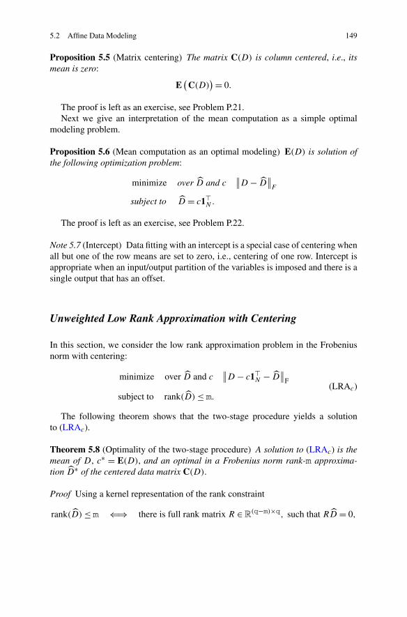
5.2 Affine Data Modeling 149
Proposition 5.5 (Matrix centering) The matrix C(D) is column centered, i.e., itsmean is zero:
E(
C(D))= 0.
The proof is left as an exercise, see Problem P.21.Next we give an interpretation of the mean computation as a simple optimal
modeling problem.
Proposition 5.6 (Mean computation as an optimal modeling) E(D) is solution ofthe following optimization problem:
minimize over D and c∥
∥D − D∥∥F
subject to D = c1�N.
The proof is left as an exercise, see Problem P.22.
Note 5.7 (Intercept) Data fitting with an intercept is a special case of centering whenall but one of the row means are set to zero, i.e., centering of one row. Intercept isappropriate when an input/output partition of the variables is imposed and there is asingle output that has an offset.
Unweighted Low Rank Approximation with Centering
In this section, we consider the low rank approximation problem in the Frobeniusnorm with centering:
minimize over D and c∥
∥D − c1�N − D∥∥F
subject to rank(D) ≤ m.(LRAc)
The following theorem shows that the two-stage procedure yields a solutionto (LRAc).
Theorem 5.8 (Optimality of the two-stage procedure) A solution to (LRAc) is themean of D, c∗ = E(D), and an optimal in a Frobenius norm rank-m approxima-tion D∗ of the centered data matrix C(D).
Proof Using a kernel representation of the rank constraint
rank(D) ≤ m ⇐⇒ there is full rank matrix R ∈R(q−m)×q, such that RD = 0,

150 5 Missing Data, Centering, and Constraints
we have the following equivalent problem to (LRAc)
minimize over D, c, and R ∈R(q−m)×q ∥
∥D − c1�N − D∥∥2
F
subject to RD = 0 and RR� = Iq−m.(LRAc,R)
The Lagrangian of (LRAc,R) is
L(
D,c,R,Λ,Ξ) :=
q∑
i=1
N∑
j=1
(
dij − ci −dij
)2
+ 2 trace(
RDΛ)+ trace
(
Ξ(
I − RR�)).
Setting the partial derivatives of L to zero, we obtain the necessary optimality con-ditions
∂L/∂D = 0 =⇒ D − c1�N − D = R�Λ�, (L1)
∂L/∂c = 0 =⇒ Nc = (D − D)1N, (L2)
∂L/∂R = 0 =⇒ DΛ = R�Ξ, (L3)
∂L/∂Λ = 0 =⇒ RD = 0, (L4)
∂L/∂Ξ = 0 =⇒ RR� = I. (L5)
The theorem follows from the system of (L1–L5). Next we list the derivation steps.From (L3), (L4), and (L5), it follows that Ξ = 0, and from (L1) we obtain
D − D = c1�N + R�Λ�.
Substituting the last identity in (L2), we have
Nc = (c1�N + R�Λ�)1N = Nc + R�Λ�1N =⇒ R�Λ�1N = 0
=⇒ Λ�1N = 0.
Multiplying (L1) from the left by R and using (L4) and (L5), we have
R(
D − c1�N
)= Λ�. (∗)
Now, multiplication of the last identity from the right by 1N and use of Λ�1N = 0,shows that c is the row mean of the data matrix D,
R(
D1N − Nc)= 0 =⇒ c = 1
ND1N.
Next, we show that D is an optimal in a Frobenius norm rank-m approximationof D − c1�
N . Multiplying (L1) from the right by Λ and using DΛ = 0, we have(
D − c1�N
)
Λ = R�Λ�Λ. (∗∗)

5.2 Affine Data Modeling 151
Defining
Σ :=√
Λ�Λ and V := ΛΣ−1,
(∗) and (∗∗) become
R(
D − c1�N
)= ΣV �, V �V = I
(
D − c1�N
)
V = R�Σ, RR� = I.
The above equations show that the rows of R and the columns of V span, respec-tively, left and right m-dimensional singular subspaces of the centered data matrixD − c1�
N . The optimization criterion is minimization of
∥
∥D − D − c1�N
∥
∥
F = ∥∥R�Λ�∥∥
F =√
trace(
ΛΛ�)= trace(Σ).
Therefore, a minimum is achieved when the rows of R and the columns of V spanthe, respectively, left and right m-dimensional singular subspaces of the centereddata matrix D − c1�
N , corresponding to the m smallest singular values. The solutionis unique if and only if the mth singular value is strictly bigger than the (m+ 1)stsingular value. Therefore, D is a Frobenius norm optimal rank-m approximation ofthe centered data matrix D − c1�
N , where c = D1N/N . �
Theorem 5.9 (Nonuniqueness) Let
D = PL, where P ∈ Rq×m and L ∈R
m×N
be a rank revealing factorization of an optimal in a Frobenius norm rank-m ap-proximation of the centered data matrix C(D). The solutions of (LRAc) are of theform
c∗(z) = E(D) + Pz
D∗(z) = P(
L − z1�N
) for z ∈Rm.
Proof
c1�N + D = c1�
N + PL
= c1�N + Pz1�
N + PL − Pz1�N
= (c + Pz)︸ ︷︷ ︸
c′1�N + P
(
L − z1�N
)
︸ ︷︷ ︸
L′
= c′1�N + D′.
Therefore, if (c, D) is a solution, then (c′, D′) is also a solution. From Theorem 5.8,it follows that c = E(D), D = PL is a solution. �
The same type of nonuniqueness appears in weighted and structured low rankapproximation problems with centering. This can cause problems in the optimiza-tion algorithms and implies that solutions produced by different methods cannot becompared directly.

152 5 Missing Data, Centering, and Constraints
Weighted Low Rank Approximation with Centering
Consider the weighted low rank approximation problem with centering:
minimize over D and c∥
∥D − D − c1�∥∥
W
subject to rank(D) ≤ m,(WLRAc)
where W is a symmetric positive definite matrix and ‖ · ‖W is the weighted norm,defined in (‖ · ‖W ). The two-stage procedure of computing the mean in a preprocess-ing step and then the weighted low rank approximation of the centered data matrix,in general, yields a suboptimal solution to (WLRAc). We present two algorithmsfor finding a locally optimal solution to (WLRAc). The first one is an alternatingprojections type method and the second one is a variable projections type method.First, however, we present a special case of (WLRAc) with analytic solution that ismore general than the case W = αI , with α �= 0.
Two-Sided Weighted Low Rank Approximation
Theorem 5.10 (Reduction to an unweighted problem) A solution to (WLRAc), inthe case
W = Wr ⊗ Wl, where Wl ∈ Rq×q and Wr ∈ R
N×N (Wr ⊗ Wl)
with Wr1N = λ1N , for some λ, is
c∗ =√
W−1l c∗
m/√
λ, D∗ =√
W−1lD∗
m
√
W−1r ,
where (c∗m, D∗
m) is a solution to the unweighted low rank approximation problemwith centering
minimize over Dm and cm∥
∥Dm − cm1�N − Dm
∥
∥
F
subject to rank(Dm) ≤ m.
for the modified data matrix Dm := √WlD
√Wr.
Proof Using the property Wr1N = λ1N of Wr, we have∥
∥D − D − c1�∥∥
W= ∥∥√Wl
(
D − D − c1�)√Wr∥
∥
F
= ∥∥Dm − Dm − cm1�∥∥
F
where
Dm =√WlD√
Wr, Dm =√WlD√
Wr, and cm =√Wlc√
λ.
Therefore, the considered problem is equivalent to the low rank approximation prob-lem (LRAc) for the modified data matrix Dm. �

5.2 Affine Data Modeling 153
Alternating Projections Algorithm
Using the image representation of the rank constraint
rank(D) ≤ m ⇐⇒ D = PL, where P ∈Rq×m and L ∈ R
m×N,
we obtain the following problem equivalent to (WLRAc)
minimize over P ∈ Rq×m, L ∈R
m×N , and c ∈ Rq∥
∥D − PL − c1�N
∥
∥
W.
(WLRAc,P )
The method is motivated by the fact that (WLRAc,P ) is linear in c and P as well asin c and L. Indeed,
∥
∥D − c1�N − PL
∥
∥
W=∥
∥
∥
∥
vec(D) − [IN ⊗ P 1N ⊗ Iq]
[
vec(L)
c
]∥
∥
∥
∥
W
=∥
∥
∥
∥
vec(D) − [L� ⊗ Iq 1N ⊗ Iq]
[
vec(P )
c
]∥
∥
∥
∥
W
.
This suggests an iterative algorithm alternating between minimization over c and P
with a fixed L and over c and L with a fixed P , see Algorithm 4. Each iteration stepis a weighted least squares problem, which can be solved globally and efficiently.The algorithm starts from an initial approximation c(0), P (0), L(0) and on each it-eration step updates the parameters with the newly computed values from the lastleast squares problem. Since on each iteration the cost function value is guaranteed
Algorithm 4 Alternating projections algorithm for weighted low rank approxima-tion with centering
Input: data matrix D ∈ Rq×N , rank constraint m, positive definite weight matrix W ∈ R
Nq×Nq,and relative convergence tolerance ε.
1: Initial approximation: compute the mean c(0) := E(D) and the rank-m approximation D(0) ofthe centered matrix D − c(0)1�
N . Let P (0) ∈ Rq×m and L(0) ∈ R
m×N are full rank matrices,such that D(0) = P (0)L(0).
2: k := 0.3: repeat4: Let P := [IN ⊗ P (k) 1N ⊗ Iq
]
and[
vec(L(k+1))
c(k+1)
]
:= (P�WP)−1P�W vec(D).
5: Let L := [L(k+1)� ⊗ Iq 1N ⊗ Iq]
and[
vec(P (k+1))
c(k+1)
]
:= (L�WL)−1L�W vec(D).
6: Let D(k+1) := P (k+1)L(k+1).7: k = k + 1.8: until ‖D(k) − D(k−1)‖W /‖D(k)‖W < ε.
Output: Locally optimal solution c := c(k) and D∗ = D(k) of (WLRAc,P ).

154 5 Missing Data, Centering, and Constraints
Fig. 5.1 Sequence of costfunction values, produced byAlgorithm 4
to be non-increasing and the cost function is bounded from below, the sequenceof cost function values, generated by the algorithm converges. Moreover, it can beshown that the sequence of parameter approximations c(k), P (k), L(k) converges toa locally optimal solution of (WLRAc,P ).
Example 5.11 Implementation of the methods for weighted and structured lowrank approximation with centering, presented in this section, are available from thebook’s web page. Figure 5.1 shows the sequence of the cost function values for arandomly generated weighted rank-1 approximation problem with q = 3 variablesand N = 6 data points. The mean of the data matrix and the approximation of themean, produced by the Algorithm 4 are, respectively
c(0) =⎡
⎣
0.50170.70680.3659
⎤
⎦ and c =⎡
⎣
0.43650.67380.2964
⎤
⎦ .
The weighted rank-1 approximation of the matrix D − c(0)1�N has approximation
error 0.1484, while the weighted rank-1 approximation of the matrix D − c1�N
has approximation error 0.1477. This proves the suboptimality of the two-stageprocedure—data centering, followed by weighted low rank approximation.
Variable Projections Algorithm
The variable projections approach is based on the observation that (WLRAc,P ) is adouble minimization problem
minimize over P ∈ Rq×m f (P )
where the inner minimization is a weighted least squares problem
f (P ) := minL∈Rm×N , c∈Rq
∥
∥D − PL − c1�N
∥
∥
W

5.2 Affine Data Modeling 155
and therefore can be solved analytically. This reduces the original problem to anonlinear least squares problem over P only. We have
f (P ) =√
vec�(D)WP(
P�WP)−1P�W vec(D),
where
P := [IN ⊗ P 1N ⊗ Iq]
.
For the outer minimization any standard unconstrained nonlinear (least squares)algorithm is used.
Example 5.12 For the same data, initial approximation, and convergence toleranceas in Example 5.11, the variable projections algorithm, using numerical approxima-tion of the derivatives in combination with quasi-Newton method converges to a lo-cally optimal solution with approximation error 0.1477—the same as the one foundby the alternating projections algorithm. The optimal parameters found by the twoalgorithms are equivalent up to the nonuniqueness of a solution (Theorem 5.9).
Hankel Low Rank Approximation with Centering
In the case of data centering we consider the following modified Hankel low rankapproximation problem:
minimize over w and c∥
∥w − c − w∥
∥
2
subject to rank(
Hn+1(w))≤ r.
(HLRAc)
Algorithm
Consider the kernel representation of the rank constraint
rank(
Hn+1(w))≤ r ⇐⇒ there is full rank matrix R ∈ R
p×(n+1)q
such that RHn+1(wd) = 0.
We have
RHn+1(w) = 0 ⇐⇒ T (R)w = 0,
where
T (R) =
⎡
⎢
⎢
⎢
⎣
R0 R1 · · · Rn
R0 R1 · · · Rn
. . .. . .
. . .
R0 R1 · · · Rn
⎤
⎥
⎥
⎥
⎦

156 5 Missing Data, Centering, and Constraints
(all missing elements are zeros). Let P be a full rank matrix, such that
(P ) = ker(
T (R))
.
Then the constraint of (HLRAc) can be replaced by
there is �, such that w = P�,
which leads to the following problem equivalent to (LRAc)
minimize over R f (R),
where
f (R) := minc,�
∥
∥
∥
∥
w − [1N ⊗ Iq P]
[
c
�
]∥
∥
∥
∥
2.
The latter is a standard least squares problem, so that the evaluation of f for agiven R can be done efficiently. Moreover, one can exploit the Toeplitz structureof the matrix T in the computation of P and in the solution of the least squaresproblem.
Example 5.13 The data sequence is
w(t) = 0.9t + 1, t = 1, . . . ,10.
The sequence (0.91, . . . ,0.910) satisfies a difference equation
σw = aw
(a first order autonomous linear time-invariant model), however, a shifted sequencew(t) = 0.9t + c, with c �= 0, does not satisfy such an equation. The mean of the datais E(w) = 1.5862, so that the centered data w(t) − E(D) are not a trajectory of afirst order autonomous linear time-invariant model. Solving the Hankel structuredlow rank approximation problem with centering (HLRAc), however, yields the exactsolution c = 1.
Preprocessing by centering the data is common in system identification. Exam-ple 5.13 shows that preprocessing can lead to suboptimal results. Therefore, thereis need for methods that combine data preprocessing with the existing identificationmethods. The algorithm derived in this section is such a method for identification inthe errors-in-variables setting. It can be modified for output error identification, i.e.,assuming that the input of the system is known exactly.
5.3 Complex Least Squares Problem with Constrained Phase
Problem Formulation
The problem considered in this section is defined as follows.

5.3 Complex Least Squares Problem with Constrained Phase 157
Problem 5.14 Given a complex valued m × n matrix A and an m × 1 vector b,find a real valued n × 1 vector x and a number φ, such that the equation’s error orresidual of the overdetermined system of linear equations
Axeiφ ≈ b (i is the imaginary unit),
is minimized in the least squares sense, i.e.,
minimize over x ∈Rn and φ ∈ (−π,π] ∥
∥Axeiφ − b∥
∥
2. (CLS)
Problem (CLS) is a complex linear least squares problem with constraint that allelements of the solution have the same phase.
As formulated, (CLS) is a nonlinear optimization problem. General purpose localoptimization methods can be used for solving it, however, this approach has theusual disadvantages of local optimization methods: need of initial approximation, noguarantee of global optimality, convergence issues, and no insight in the geometryof the solutions set. In Bydder (2010) the following closed-form solution of (CLS)is derived:
x = (�(AH A))+�(AH be−iφ), (SOL1 x)
φ = 1
2∠((
AH b)��(AH A
)+(AH b
))
, (SOL1 φ)
where �(A)/�(A) is the real/imaginary part, ∠(A) is the angle, AH is the com-plex conjugate transpose, and A+ is the pseudoinverse of A. Moreover, in the casewhen a solution of (CLS) is not unique, (SOL1 x, SOL1 φ) is a least norm ele-ment of the solution set, i.e., a solution (x,φ), such that ‖x‖2 is minimized. Ex-pression (SOL1 x) is the result of minimizing the cost function ‖Axeiφ − b‖2 withrespect to x, for a fixed φ. This is a linear least squares problems (with complexvalued data and real valued solution). Then minimization of the cost function withrespect to φ, for x fixed to its optimal value (SOL1 x), leads through a nontrivialchain of steps to (SOL1 φ).
Solution
Problem (CLS) is equivalent1 to the problem
minimize over x ∈Rn and φ′ ∈ (−π,π] ∥
∥Ax − beiφ′∥∥
2, (CLS’)
1Two optimization problems are equivalent if the solution of the first can be obtained from thesolution of the second by a one-to-one transformation. Of practical interest are equivalent problemsfor which the transformation is “simple”.

158 5 Missing Data, Centering, and Constraints
where φ′ = −φ. With
y1 := �(eiφ′)= cos(
φ′)= cos(φ) and y2 := �(eiφ′)= sin(
φ′)= − sin(φ),
we have[
�(beiφ′)
�(beiφ′)
]
=[�(b) −�(b)
�(b) �(b)
][
y1y2
]
.
Then, (CLS’) is furthermore equivalent to the problem
minimize over x ∈ Rn and y ∈ R
2∥
∥
∥
∥
[�(A)
�(A)
]
x −[�(b) −�(b)
�(b) �(b)
]
y
∥
∥
∥
∥
subject to ‖y‖2 = 1,
or
minimize over z ∈ Rn+2 z�C�Cz subject to z�D�Dz = 1, (CLS”)
with
C :=[�(A) �(b) −�(b)
�(A) �(b) �(b)
]
∈R2m×(n+2) and D :=
[
0 00 I2
]
∈R(n+2)×(n+2).
(C, D)It is well known that a solution of problem (CLS”) can be obtained from the general-ized eigenvalue decomposition of the pair of matrices (C�C,D). More specifically,the smallest generalized eigenvalue λmin of (C�C,D) is equal to the minimumvalue of (CLS”), i.e.,
λmin = ∥∥Axeiφ − b∥
∥
22.
If λmin is simple, a corresponding generalized eigenvector zmin is of the form
zmin = α
⎡
⎢
⎣
x
− cos(φ)
sin(φ)
⎤
⎥
⎦ ,
for some α ∈ R. We have the following result.
Theorem 5.15 Let λmin be the smallest generalized eigenvalue of the pair of ma-trices (C�C,D), defined in (C, D), and let zmin be a corresponding generalizedeigenvector. Assuming that λmin is a simple eigenvalue, problem (CLS) has uniquesolution, given by
x = 1
‖z2‖2z1, φ = ∠(−z2,1 + iz2,2), where zmin =:
[
z1z2
] }
n}
2. (SOL2)

5.3 Complex Least Squares Problem with Constrained Phase 159
Remarks
1. Generalized eigenvalue decomposition vs. generalized singular value decompo-sition Since the original data are the matrix A and the vector b, the generalizedsingular value decomposition of the pair (C,D) can be used instead of the gen-eralized eigenvalue decomposition of the pair (C�C,D). This avoids “squaring”the data and is recommended from a numerical point of view.
2. Link to low rank approximation and total least squares Problem (CLS”) isequivalent to the generalized low rank approximation problem
minimize over C ∈ R2m×(n+2)
∥
∥(C − C)D∥
∥
F
subject to rank(C) ≤ n + 1 and CD⊥ = CD⊥,(GLRA)
where
D⊥ =[
In 00 0
]
∈R(n+2)×(n+2)
and ‖ · ‖F is the Frobenius norm. Indeed, the constraints of (GLRA) imply that∥
∥
(
C − C)D∥∥F = ∥∥b −b∥∥2, whereb = Axeiφ.
The normalization (SOL2) is reminiscent to the generic solution of the total leastsquares problems. The solution of total least squares problems, however, involvesa normalization by scaling with the last element of a vector zmin in the approxi-mate kernel of the data matrix C, while the solution of (CLS) involves normal-ization by scaling with the norm of the last two elements of the vector zmin.
3. Uniqueness of the solution and minimum norm solutions A solution x of (CLS)is nonunique when A has nontrivial null space. This source of nonuniqueness isfixed in Bydder (2010) by choosing from the solutions set a least norm solution.A least norm solution of (CLS), however, may also be nonunique due to possiblenonuniquess of φ. Consider the following example,
A =[
1 i−i 1
]
, b =[
1−i
]
,
which has two least norm solutions
xeiφ1 =[
10
]
and x′eiφ2 =[
0−i
]
.
Moreover, there is a trivial source of nonuniqueness in x and φ due to
xeiφ = −xei(φ±π)
with both φ and one of the angles φ ± π in the interval (−π,π].

160 5 Missing Data, Centering, and Constraints
Computational Algorithms
Solution (SOL1 x, SOL1 φ) gives a straightforward procedure for computing a leastnorm solution of problem (CLS).
160a 〈Complex least squares, solution by (SOL1 x, SOL1 φ) 160a〉≡function cx = cls1(A, b)invM = pinv(real(A’ * A)); Atb = A’ * b;phi = 1 / 2 * angle((Atb).’ * invM * Atb);x = invM * real(Atb * exp(-i * phi));cx = x * exp(i * phi);
Defines:cls1, used in chunk 163b.
The corresponding computational cost is
cls1 — O(
n2m + n3).
Theorem 5.15 gives two alternative procedures—one based on the generalizedeigenvalue decomposition:
160b 〈Complex least squares, solution by generalized eigenvalue decomposition 160b〉≡function cx = cls2(A, b)〈define C, D, and n 160c〉[v, l] = eig(C’ * C, D); l = diag(l);l(find(l < 0)) = inf; % ignore nevative values[ml, mi] = min(l); z = v(:, mi);phi = angle(-z(end - 1) + i * z(end));x = z(1:(end - 2)) / norm(z((end - 1):end));cx = x * exp(i * phi);
Defines:cls2, used in chunk 163b.
160c 〈define C, D, and n 160c〉≡ (160 161)C = [real(A) real(b) -imag(b);
imag(A) imag(b) real(b)];n = size(A, 2); D = diag([zeros(1, n), 1, 1]);
and the other one based on the generalized singular value decomposition:
160d 〈Complex least squares, solution by generalized singular value decomposition 160d〉≡function cx = cls3(A, b)〈define C, D, and n 160c〉[u, v] = gsvd(C, D); z = v(:, 1);phi = angle(-z(end - 1) + i * z(end));x = pinv(C(:, 1:n)) * [real(b * exp(- i * phi));
imag(b * exp(- i * phi))];cx = x * exp(i * phi);
Defines:cls3, used in chunk 163b.

5.3 Complex Least Squares Problem with Constrained Phase 161
The computational costs are
cls2 — O(
(n + 2)2m + (n + 2)3)
and
cls3 — O(
m3 + (n + 2)2m2 + (n + 2)2m + (n + 2)3).
Note, however, that cls2 and cls3 compute the full generalized eigenvaluedecomposition and generalized singular value decomposition, respectively, whileonly the smallest generalized eigenvalue/eigenvector or singular value/singular vec-tor pair is needed for solving (CLS). This suggests a way of reducing the computa-tional complexity by a factor of magnitude.
The equivalence between problem (CLS) and the generalized low rank approxi-mation problem (GLRA), noted in remark 2 above, allows us to use the algorithmfrom Golub et al. (1987) for solving problem (CLS). The resulting Algorithm 5 isimplemented in the function cls4.
161 〈Complex least squares, solution by Algorithm 5 161〉≡function cx = cls4(A, b)〈define C, D, and n 160c〉R = triu(qr(C, 0));[u, s, v] = svd(R((n + 1):(n + 2), (n + 1):end));phi = angle(v(1, 2) - i * v(2, 2));x = R(1:n, 1:n)
\ (R(1:n, (n + 1):end) * [v(1, 2); v(2, 2)]);cx = x * exp(i * phi);
Defines:cls4, used in chunk 163b.
Its computational cost is
cls4 — O(
(n + 2)2m)
.
A summary of the computational costs for the methods, implemented in the func-tions cls1-4, is given in Table 5.5.
Algorithm 5 Solution of problem (CLS) using generalized low rank approximation
Input: A ∈ Cm×n, b ∈ C
m×1
1: QR factorization of C, QR = C.
2: Define R =:[
R11 R120 R22
]
}
n}
2, where R11 ∈ R
n×n.
3: Singular value decomposition of R22, UΣV � = R22.
4: Let φ := ∠(v12 − iv22) and x := R−111 R12
[
v12v22
]
.
Output: xeiφ

162 5 Missing Data, Centering, and Constraints
Table 5.5 Summary of methods for solving the complex least squares problem (CLS)
Function Method Computational cost
cls1 (SOL1 x, SOL1 φ) O(n2m + n3)
cls2 full generalized eigenvalue decomp. O((n + 2)2m + (n + 2)3)
cls3 full generalized singular value decomp. O(m3 + (n + 2)2m2 + (n + 2)2m + (n + 2)3)
cls4 Algorithm 5 O((n + 2)2m)
Fig. 5.2 Computation time for the four methods, implemented in the functions cls1, . . . , cls4
Numerical Examples
Generically, the four solution methods implemented in the functions cls1, . . . ,cls4 compute the same result, which is equal to the unique solution of prob-lem (CLS). As predicted by the theoretical computation costs, the method based onAlgorithm 5 is the fastest of the four methods when both the number of equationsand the number of unknowns is growing, see Fig. 5.2.
The figures are generated by using random test data
162a 〈Computation time for cls1-4 162a〉≡ 162b�〈initialize the random number generator 89e〉mm = 1000; nm = 1000; s = {’b-’ ’g-.’ ’r:’ ’c-’};Am = rand(mm, nm) + i * rand(mm, nm);bm = rand(mm, 1 ) + i * rand(mm, 1 );
Defines:test_cls, never used.
and solving problems with increasing number of equations m
162b 〈Computation time for cls1-4 162a〉+≡ �162a 163a�Nm = 10; M = round(linspace(500, 1000, Nm)); n = 200;for j = 1:Nm, m = M(j); 〈call cls1-4 163b〉 endk = 1; x = M; ax = [500 1000 0 0.5]; name = ’cls-f1’;〈plot cls results 163c〉

5.4 Approximate Low Rank Factorization with Structured Factors 163
as well as increasing number of unknowns n
163a 〈Computation time for cls1-4 162a〉+≡ �162bNn = 10; N = round(linspace(100, 700, Nn)); m = 700;for j = 1:Nn, n = N(j); 〈call cls1-4 163b〉 endk = 2; x = N; ax = [100 700 0 6]; name = ’cls-f2’;〈plot cls results 163c〉
163b 〈call cls1-4 163b〉≡ (162b 163a)A = Am(1:m, 1:n); b = bm(1:m);for i = 1:4 % cls1, cls2, cls3, cls4eval(sprintf(’tic, x = cls%d(A, b); t(%d) = toc;’, i, i))
endT(:, j) = t’;
Uses cls1 160a, cls2 160b, cls3 160d, and cls4 161.
163c 〈plot cls results 163c〉≡ (162b 163a)figure(k), hold onfor i = 1:4 plot(x, T(i, :), s{i}, ’linewidth’, 2), endlegend(’cls1’, ’cls2’, ’cls3’, ’cls4’)for i = 1:4, plot(x, T(i, :), [s{i}(1) ’o’]), endaxis(ax), print_fig(name)
Uses print_fig 25a.
5.4 Approximate Low Rank Factorization with StructuredFactors
Problem Formulation
Rank Estimation
Consider an q× N real matrix D0 with rank m0 < q and let
D0 = P0L0, where P0 ∈ Rq×m0 and L0 ∈R
m0×N
be a rank revealing factorization of D0. Suppose that instead of D0 a matrix
D := D0 + D
is observed, where D is a perturbation, e.g., D can represent rounding errors in afinite precision arithmetic or measurement errors in data acquisition. The rank ofthe perturbed matrix D may not be equal to m0. If D is random, generically, D isfull rank, so that from a practical point of view, a nonzero perturbation D makesthe matrix D full rank. If, however, D is “small”, in the sense that its Frobeniusnorm ‖D‖F is less than a constant ε (defining the perturbation size), then D will be

164 5 Missing Data, Centering, and Constraints
“close” to a rank-m0 matrix in the sense that the distance of D to the manifold ofrank-m0 matrices
dist(D,m0) := minD
∥
∥D − D∥∥F subject to rank(
D)= m0 (5.12)
is less than the perturbation size ε. Therefore, provided that the size ε of the pertur-bation D is known, the distance measure dist(D,m), for m= 1,2, . . . , can be usedto estimate the rank of the unperturbed matrix as follows
m= arg min{
m | dist(D,m) < ε}
.
Problem (5.12) has analytic solution in terms of the singular values σ1, . . . , σqof D
dist(D,m0) :=√
σ 2m0+1 + · · · + σ 2
q ,
and therefore the rank of D0 can be estimated from the decay of the singular valuesof D (find the largest singular value that is sufficiently small compared to the per-turbation size ε). This is the standard way for rank estimation in numerical linearalgebra, where the estimate m is called numerical rank of D, cf., p. 38. The questionoccurs:
Given a perturbed matrix D := D0 + D, is the numerical rank of D the “best”estimate for the rank of D0, and if so, in what sense?
The answer to the above question depends on the type of the perturbation D.If D is a random matrix with zero mean elements that are normally distributed,independent, and with equal variances, then the estimate D, defined by (5.12) isa maximum likelihood estimator of D0, i.e., it is statistically optimal. If, however,one or more of the above assumptions are not satisfied, D is not optimal and canbe improved by modifying problem (5.12). Our objective is to justify this statementin a particular case when there is prior information about the true matrix D0 in theform of structure in a normalized rank-revealing factorization and the elements ofthe perturbation D are independent but possibly with different variances.
Prior Knowledge in the Form of Structure
In applications often there is prior knowledge about the unperturbed matrix D0,apart from the basic one that D0 is rank deficient. Whenever available, suchprior knowledge is beneficial to use in the computation of the distance measuredist(D,m). Using the prior knowledge amounts to modification of problem (5.12).For example, common prior information in image and text classification is nonneg-ativity of the elements of D0. In this case, we require the approximation D to be

5.4 Approximate Low Rank Factorization with Structured Factors 165
nonnegative and in order to achieve this, we impose nonnegativity of the estimate Das an extra constraint in (5.12). Similarly, in signal processing and system theory thematrix D0 is Hankel or Toeplitz structured and the relevant modification of (5.12)is to constrain D to have the same structure. In chemometrics, the measurement er-rors dij may have different variances σ 2vij , which are known (up to a scaling factor)from the measurement setup or from repeated experiments. Such prior informationamounts to changing the cost function ‖D − D‖F to the weighted norm ‖D − D‖Σ
of the error matrix D − D, where the elements of the weight matrix Σ are up toa scaling factor equal to the inverse square root of the error variance σ 2V . In gen-eral, either the addition of constraints on D or the replacement of the Frobeniusnorm with a weighted norm, renders the modified distance problem (5.12) difficultto solve. A globally optimal solution can no longer be given in terms of the singularvalues of D and the resulting optimization problem is nonconvex.
A factorization D = PL is nonunique; for any r × r nonsingular matrix T , weobtain a new factorization D = P ′L′, where P ′ := PT −1 and L′ = T L. Obviously,this imposes a problem in estimating the factors P and L from the data D. In orderto resolve the nonuniqueness problem, we assume that
P =[
ImP ′]
.
Next, we present an algorithm for approximate low rank factorization with struc-tured factors and test its performance on synthetic data. We use the alternating pro-jections approach, because it is easier to modify for constrained optimization prob-lems. Certain constrained problems can be treated also using a modification of thevariable projections.
Statistical Model and Maximum Likelihood Estimation Problem
Consider the errors-in-variables model
D = D0 + D, where D0 = P0L0, with
P0 ∈Rq×m, L0 ∈ R
m×N, m< q
and vec(D) ∼ N(
0, σ 2 diag(v))
.
(EIV0)
The true data matrix D0 has rank equal to m and the measurement errors dij are zeromean, normal, and uncorrelated, with covariance σ 2vi+q(j−1). The vector v ∈ R
qN
specifies the element-wise variances of the measurement error matrix D up to anunknown factor σ 2.
In order to make the parameters P0 and L0 unique, we impose the normalizationconstraint (or assumption on the “true” parameter values)
P0 =[
ImP ′
0
]
. (A1)

166 5 Missing Data, Centering, and Constraints
In addition, the block P ′0 of P0 has elements (specified by a selector matrix S) equal
to zero
S vec(
P ′0
)= 0. (A2)
The parameter L0 is periodic with a period l ∈ Z+
L0 = 1�l ⊗ L′
0, (A3)
nonnegative
L′0 ≥ 0, (A4)
and with smooth rows in the sense that∥
∥L′0D∥
∥
2F ≤ δ, (A5)
where δ > 0 is a smoothness parameter and D is a finite difference matrix
D :=
⎡
⎢
⎢
⎢
⎣
1 −1−1 1
. . .. . .
−1 1
⎤
⎥
⎥
⎥
⎦
.
Define the q× N matrix
Σ = vec−1([
v−1/21 · · · v
−1/2qN
])
:=
⎡
⎢
⎢
⎢
⎢
⎢
⎢
⎣
v−1/21 v
−1/2q+1 · · · v
−1/2q(N−1)+1
v−1/22 v
−1/2q+2 · · · v
−1/2q(N−1)+2
......
. . ....
v−1/2q v
−1/22q · · · v
−1/2qN
⎤
⎥
⎥
⎥
⎥
⎥
⎥
⎦
. (Σ)
The maximum likelihood estimator for the parameters P0 and L0 in (EIV0) underassumptions (A1–A5), with known parameters m, v, S, and δ, is given by the fol-lowing optimization problem:
minimize over P ′, L′, and D∥
∥D − D∥∥2Σ
(cost function) (C0)
subject to D = CP (rank constraint)
P =[
ImP ′]
(normalization of P ) (C1)
S vec(
P ′)= 0 (zero elements of P ′) (C2)
L = 1�l ⊗ L′ (periodicity of L) (C3)
L′ ≥ 0 (nonnegativity of L) (C4)∥
∥L′D∥
∥
2F ≤ δ (smoothness of L) (C5)

5.4 Approximate Low Rank Factorization with Structured Factors 167
The rank and measurement errors assumptions in the model (EIV0) imply theweighted low rank approximation nature of the estimation problem (C0–C5) withweight matrix given by (Σ). Furthermore, the assumptions (A1–A5) about the truedata matrix D0 correspond to the constraints (C1–C5) in the estimation problem.
Computational Algorithm
Algorithm 6 Alternating projections algorithm for solving problem (C0–C5)
• Find an initial approximation (P ′(0),L′(0)).• For k = 0,1, . . . till convergence do
1. P ′(k+1) := arg minP ′ ‖D − PL‖2Σ subject to (C1–C2) with L′ = L′(k)
2. L′(k+1) := arg minL′ ‖D − PL‖2Σ subject to (C3–C5) with P ′ = P ′(k+1)
The alternating projections algorithm, see Algorithm 6, is based on the observa-tion that the cost function (C0) is quadratic and the constraints (C1–C5) are linearin either P or L. Therefore, for a fixed value of P , (C0–C5) is a nonnegativity con-strained least squares problem in L and vice verse, for a fixed value of L, (C0–C5)is a constrained least squares problem in P . These problems correspond to, respec-tively, steps 1 and 2 of the algorithm. Geometrically they are projections. In theunweighted (i.e., Σ = 1q1�
N ) and unconstrained case, the problem on step 1 is theorthogonal projection
D = DL�(LL�)−1L� = DΠL
of the row of D on the span of the rows of L, and problem on step 2 is the orthogonalprojection
D = P(
P �P)−1
P �D = ΠP D
of the columns of D on the span of the column of P . The algorithm iterates the twoprojections.
Note 5.16 (Rank deficient factors P and L) If the factor L is rank deficient, the in-dicated inverse in the computation of the projected matrix P ∗ does not exist. (Thishappens when the rank of the approximation D if less than m.) The projection P ∗,however, is still well defined by the optimization problem on step 1 of the algo-rithm and can be computed in closed form by replacing the inverse with the pseudoinverses. The same is true when the factor L is rank deficient.
Theorem 5.17 Algorithm 6 is globally and monotonically convergent in the ‖ · ‖Σ
norm, i.e., if
D(k) := P (k)L(k)

168 5 Missing Data, Centering, and Constraints
is the approximation on the kth step of the algorithm, then
f (k) := ∥∥D − D(k)∥
∥
2Σ
→ f ∗, as k → ∞. (f (k) → f ∗)
Assuming that there exists a solution to the problem (C0–C5) and any (locally op-timal) solution is unique (i.e., it is a strict minimum), the sequences D(k), P (k),and L(k) converge element-wise, i.e.,
D(k) → D∗, P (k) → P ∗, and L(k) → L∗, as k → ∞, (D(k) → D∗)
where D∗ := P ∗L∗ is a (locally optimal) solution of (C0–C5).
The proof is given in Appendix B.
Simulation Results
In this section, we show empirically that exploiting prior knowledge ((Σ ) and as-sumptions (A1–A5)) improves the performance of the estimator. The data matrix D
is generated according to the errors-in-variables model (EIV0) with parametersN = 100, q= 6, and m= 2. The true low rank matrix D0 = P0L0 is random and theparameters P0 and L0 are normalized according to assumption (A1) (so that theyare unique). For the purpose of validating the algorithm, the element p0,qN is set tozero but this prior knowledge is not used in the parameter estimation.
The estimation algorithm is applied on M = 100 independent noise realizationsof the data D. The estimated parameters on the ith repetition are denoted by P (i),L(i) and D(i) := P (i)L(i). The performance of the estimator is measured by thefollowing average relative estimation errors:
eD = 1
M
M∑
i=1
‖D0 − D(i)‖2F
‖D0‖2F
, eP = 1
M
M∑
i=1
‖P0 − P (i)‖2F
‖P0‖2F
,
eL = 1
M
M∑
i=1
‖L0 − L(i)‖2F
‖L0‖2F
, and ez = 1
M
M∑
i=1
∣
∣p(i)qN
∣
∣.
For comparison the estimation errors are reported for the low rank approximationalgorithm, using only the normalization constraint (A1), as well as for the proposedalgorithm, exploiting the available prior knowledge. The difference between the twoestimation errors is an indication of how important is the prior knowledge in theestimation.
Lack of prior knowledge is reflected by specific choice of the simulation param-eters as follows:

5.4 Approximate Low Rank Factorization with Structured Factors 169
Fig. 5.3 Effect of weighting ( —exploiting prior knowledge, —without ex-ploiting prior knowledge, vertical bars—standard deviations)
homogeneous errors ↔ Σ = ones(q,N)
no periodicity ↔ l = 1no zeros in P ′ ↔ S = []no sign constraint on L′ ↔ nonneg= 0
We perform the following experiments:
Σ l S = [] nonneg
rand(q,N) 1 yes 0ones(q,N) 3 yes 0ones(q,N) 1 no 0ones(q,N) 1 yes 1rand(q,N) 3 no 1
which test individually the effect of (Σ ), assumptions (A2), (A3), (A4), and theircombined effect on the estimation error. Figures 5.3–5.7 show the average rela-tive estimation errors ( is the estimator that exploits prior knowledge and
is the estimator that does not exploit prior knowledge) versus the mea-surement noise standard deviation σ , for the five experiments. The vertical bars on

170 5 Missing Data, Centering, and Constraints
Fig. 5.4 Effect of periodicity of L ( —exploiting prior knowledge, —withoutexploiting prior knowledge, vertical bars—standard deviations)
the plots visualize the standard deviation of the estimates. The results indicate thatmain factors for the improved performance of the estimator are:
1. assumption (A3)—known zeros in the P ′0 and
2. (Σ )—known covariance structure of the measurement noise.
Files reproducing the numerical results and figures presented are available from thebook’s web page.
Implementation of Algorithm 6
Initial Approximation
For initial approximation (P ′(0),L′(0)) we choose the normalized factors of a rankrevealing factorization of the solution D of (5.12). Let
D = UΣV �

5.4 Approximate Low Rank Factorization with Structured Factors 171
Fig. 5.5 Effect of zero elements in P ( —exploiting prior knowledge,—without exploiting prior knowledge, vertical bars—standard deviations)
be the singular value decomposition of D and define the partitioning
U =:m q− m[
U1 U2]
, Σ =:m q− m[
Σ1 00 Σ2
]
mq− m
, V =:m N − m[
V1 V2]
.
Furthermore, let[
U11U21
]
:= U, with U11 ∈ Rm×m.
Then
P ′(0) := U21U−111 and L(0) := U11ΣV �
define the Frobenius-norm optimal unweighted and unconstrained low rank approx-imation
D(0) :=[
I
P ′(0)
]
L(0).
More sophisticated choices for the initial approximation that take into account theweight matrix Σ are described in Sect. 2.4.

172 5 Missing Data, Centering, and Constraints
Fig. 5.6 Effect of nonnegativity of L ( —exploiting prior knowledge,—without exploiting prior knowledge, vertical bars—standard deviations)
Separable Least Squares Problem for P
In the weighted case, the projection on step 1 of the algorithm is computed sepa-rately for each row pi of P . Let di be the ith row of D and wi be the ith row of Σ .The problem
minimize over P ‖D − PL‖2Σ subject to (C1–C2)
is equivalent to the problem
minimize over pi∥
∥
(
di − piL)
diag(
wi)∥
∥
22
subject to (C1–C2), for i = 1, . . . ,m.(∗)
The projection on step 2 of the algorithm is not separable due to constraint (C5).
Taking into Account Constraint (C1)
Since the first m rows of P are fixed, we do not solve (∗) for i = 1, . . . ,m, but define
pi := e�i , for i = 1, . . . ,m,
where ei is the ith unit vector (the ith column of the identity matrix Im).

5.4 Approximate Low Rank Factorization with Structured Factors 173
Fig. 5.7 Effect of weighting, periodicity, and nonnegativity of L, and zero elements in P (—exploiting prior knowledge, —without exploiting prior knowledge, vertical
bars—standard deviations)
Taking into Account Constraint (C2)
Let Si be a selector matrix for the zeros in the ith row of P
S vec(P ′) = 0 ⇐⇒ piSi = 0, for i = m+ 1, . . . ,q.
(If there are no zeros in the ith row, then Si is skipped.) The ith problem in (∗)becomes
minimize over pi∥
∥
(
di − piL)
diag(
wi)∥
∥
22 subject to piSi = 0. (∗∗)
Let the rows of the matrix Ni form a basis for the left null space of Si . Then piSi = 0if and only if pi = ziNi , for certain zi , and problem (∗∗) becomes
minimize over zi
∥
∥
(
di − ziNiL)
diag(
wi)∥
∥
22.
Therefore, the solution of (∗) is
pi,∗ = diL�N�i
(
NiLL�N�i
)−1Ni.

174 5 Missing Data, Centering, and Constraints
Note 5.18 It is not necessary to explicitly construct the matrices Si and computebasis Ni for their left null spaces. Since Si is a selector matrix, it is a submatrix ofthe identity matrix Im. The rows of the complementary submatrix of Im form a basisfor the left null space of Si . This particular matrix Ni is also a selector matrix, sothat the product NiL need not be computed explicitly.
Taking into Account Constraint (C3)
We have,
D − PL = D − P(
1�l ⊗ L′)= [D1 · · · Dl
]− P[
L′ · · · L′]
=⎡
⎢
⎣
D1...
Dl
⎤
⎥
⎦−⎡
⎢
⎣
P...
P
⎤
⎥
⎦L′ =: D′ − (1l ⊗ P)︸ ︷︷ ︸
P ′L′ = D′ − P ′L′.
Let
Σ ′ :=⎡
⎢
⎣
Σ1...
Σl
⎤
⎥
⎦ , where Σ =: [Σ1 · · · ΣN
]
.
Then the problem
minimize over L ‖D − PL‖2Σ subject to (C3–C5)
is equivalent to the problem
minimize over L′ ‖D′ − P ′L′‖2Σ ′ subject to (C4–C5).
Taking into Account Constraint (C4)
Adding the nonnegativity constraint changes the least squares problem to a nonneg-ative least squares problem, which is a standard convex optimization problem forwhich robust and efficient methods and software exist.
Taking into Account Constraint (C5)
The problem
minimize over L ‖D − PL‖2Σ subject to ‖LD‖2
F ≤ δ
is equivalent to a regularized least squares problem
minimize over L ‖D − PL‖2Σ + γ ‖LD‖2
F

5.5 Notes 175
for certain regularization parameter γ . The latter problem is equivalent to the stan-dard least squares problem
minimize over L
∥
∥
∥
∥
[
diag(
vec(Σ))
vec(D)
0
]
−[
diag(
vec(Σ))
(I ⊗ P )√γ (D� ⊗ I )
]
vec(L)
∥
∥
∥
∥
2
2.
Stopping Criteria
The iteration is terminated when the following stopping criteria are satisfied∥
∥P (k+1)L(k+1) − P (k)L(k)∥
∥
Σ/∥
∥P (k+1)L(k+1)∥
∥
Σ< εD,
∥
∥
(
P (k+1) − P (k))
L(k+1)∥
∥
Σ/∥
∥P (k+1)L(k+1)∥
∥
Σ< εP , and
∥
∥L(k+1)(
L(k+1) − L(k))∥
∥
Σ/∥
∥P (k+1)L(k+1)∥
∥
Σ< εL.
Here εD , εP , and εL are user defined relative convergence tolerances for D, P ,and L, respectively.
5.5 Notes
Missing Data
Optimization methods for solving weighted low rank approximation problems withnonsingular weight matrix have been considered in the literature under differentnames:
• criss-cross multiple regression (Gabriel and Zamir 1979),• Riemannian singular value decomposition (De Moor 1993),• maximum likelihood principal component analysis (Wentzell et al. 1997),• weighted low rank approximation (Manton et al. 2003), and• weighted low rank approximation (Markovsky et al. 2005).
Gabriel and Zamir (1979) consider an element-wise weighted low rank approxi-mation problem with diagonal weight matrix W , and propose an iterative solutionmethod. Their method, however, does not necessarily converge to a minimum point,see the discussion in Gabriel and Zamir (1979, Sect. 6, p. 491). Gabriel and Zamir(1979) proposed an alternating projections algorithm for the case of unweighted ap-proximation with missing values, i.e., wij ∈ {0,1}. Their method was further gener-alized by Srebro (2004) for arbitrary weights.
The Riemannian singular value decomposition framework of De Moor (1993)includes the weighted low rank approximation problem with rank specificationr = min(m,n) − 1 and a diagonal weight matrix W as a special case. In De Moor(1993), an algorithm resembling the inverse power iteration algorithm is proposed.The method, however, has no proven convergence properties.

176 5 Missing Data, Centering, and Constraints
Manton et al. (2003) treat the problem as an optimization over a Grassman man-ifold and propose steepest decent and Newton type algorithms. The least squaresnature of the problem is not exploited in this work and the proposed algorithms arenot globally convergent.
The maximum likelihood principal component analysis method of Wentzell et al.(1997) is developed for applications in chemometrics, see also (Schuermans et al.2005). This method is an alternating projections algorithm. It applies to the generalweighted low rank approximation problems and is globally convergent. The conver-gence rate, however, is linear and the method could be rather slow when the r + 1stand the r th singular values of the data matrix D are close to each other. In the un-weighted case this situation corresponds to lack of uniqueness of the solution, cf.,Theorem 2.23. The convergence properties of alternating projections algorithms arestudied in Krijnen (2006), Kiers (2002).
An implementation of the singular value thresholding method in MATLAB isavailable at http://svt.caltech.edu/. Practical methods for solving the recommendersystem problem are given in Segaran (2007). The MovieLens data set is availablefrom GroupLens (2009).
Nonnegative Low Rank Approximation
The notation D ≥ 0 is used for a matrix D ∈Rq×N whose elements are nonnegative.
A low rank approximation problem with element-wise nonnegativity constraint
minimize over D∥
∥D − D∥∥subject to rank(D) ≤ m and D ≥ 0
(NNLRA)
arises in Markov chains (Vanluyten et al. 2006) and image mining (Lee and Seung1999). Using the image representation, we obtain the following problem
minimize over D, P ∈Rq×m, and L ∈ R
m×N ‖D − D‖subject to D = PL and P,L ≥ 0,
(NNLRAP )
which is a relaxation of problem (NNLRA). The minimal m, for which (NNLRAP )has a solution, is called the positive rank of D (Berman and Shaked-Monderer2003). In general, the positive rank is less than or equal to the rank.
Note that due to the nonnegativity constraint on D, the problem cannot be solvedusing the variable projections method. (There is no closed-form solution for theequivalent problem with D eliminated.) The alternating projections algorithm, how-ever, can be used almost without modification for the solution of the relaxed prob-lem (NNLRAP ). Let the norm ‖ · ‖ in (NNLRA) be the Frobenius norm. (In thecontext of Markov chains more adequate is the choice of the Kullback–Leibler di-vergence as a distance measure between D and D.) Then at each iteration step of thealgorithm two least squares problems with nonnegativity constraint (i.e., standard

References 177
optimization problems) are solved. The resulting alternating least squares algorithmis Algorithm 7.
Algorithm 7 Alternating projections algorithm for nonnegative low rank approxi-mationInput: Data matrix D, desired rank m, and convergence tolerance ε.1: Set k := 0 and compute an initial approximation D(0) := P (0)L(0) from the singular value
decomposition by setting all negative elements to zero.2: repeat3: k := k + 1.4: Solve: L(k) := arg minL ‖D − P (k−1)L‖ subject to L ≥ 0.5: Solve: P (k) := arg minP ‖D − PL(k)‖ subject to P ≥ 0.6: until ‖P (k−1)L(k−1) − P (k)L(k)‖ < ε
Output: A locally optimal solution D∗ := P (k)L(k) to problem (NNLRAP ).
References
Berman A, Shaked-Monderer N (2003) Completely positive matrices. World Scientific, SingaporeBydder M (2010) Solution of a complex least squares problem with constrained phase. Linear
Algebra Appl 433(11–12):1719–1721Cai JF, Candés E, Shen Z (2009) A singular value thresholding algorithm for matrix completion.
www-stat.stanford.edu/~candes/papers/SVT.pdfCandés E, Recht B (2009) Exact matrix completion via convex optimization. Found Comput Math
9:717–772De Moor B (1993) Structured total least squares and L2 approximation problems. Linear Algebra
Appl 188–189:163–207Gabriel K, Zamir S (1979) Lower rank approximation of matrices by least squares with any choice
of weights. Technometrics 21:489–498Golub G, Hoffman A, Stewart G (1987) A generalization of the Eckart–Young–Mirsky matrix
approximation theorem. Linear Algebra Appl 88/89:317–327GroupLens (2009) Movielens data sets. www.grouplens.org/node/73Kiers H (2002) Setting up alternating least squares and iterative majorization algorithms for solving
various matrix optimization problems. Comput Stat Data Anal 41:157–170Krijnen W (2006) Convergence of the sequence of parameters generated by alternating least
squares algorithms. Comput Stat Data Anal 51:481–489Lee D, Seung H (1999) Learning the parts of objects by non-negative matrix factorization. Nature
401:788–791Manton J, Mahony R, Hua Y (2003) The geometry of weighted low-rank approximations. IEEE
Trans Signal Process 51(2):500–514Markovsky I, Rastello ML, Premoli A, Kukush A, Van Huffel S (2005) The element-wise weighted
total least squares problem. Comput Stat Data Anal 50(1):181–209Schuermans M, Markovsky I, Wentzell P, Van Huffel S (2005) On the equivalence between total
least squares and maximum likelihood PCA. Anal Chim Acta 544:254–267Segaran T (2007) Programming collective intelligence: building smart Web 2.0 applications.
O’Reilly MediaSrebro N (2004) Learning with matrix factorizations. PhD thesis, MITVanluyten B, Willems JC, De Moor B (2006) Matrix factorization and stochastic state representa-
tions. In: Proc 45th IEEE conf on dec and control, San Diego, California, pp 4188–4193Wentzell P, Andrews D, Hamilton D, Faber K, Kowalski B (1997) Maximum likelihood principal
component analysis. J Chemom 11:339–366

Chapter 6Nonlinear Static Data Modeling
6.1 A Framework for Nonlinear Static Data Modeling
Introduction
Identifying a curve in a set of curves that best fits given data points is a commonproblem in computer vision, statistics, and coordinate metrology. More abstractly,approximation by Fourier series, wavelets, splines, and sum-of-exponentials are alsocurve-fitting problems. In the applications, the fitted curve is a model for the dataand, correspondingly, the set of candidate curves is a model class.
Data modeling problems are specified by choosing a model class and a fitting cri-terion. The fitting criterion is maximization of a measure for fit between the data anda model. Equivalently, the criterion can be formulated as minimization of a measurefor lack of fit (misfit) between the data and a model. Data modeling problems can beclassified according to the type of model and the type of fitting criterion as follows:
• linear/affine vs. nonlinear model class,• algebraic vs. geometric fitting criterion.
A model is a subset of the data space. The model is linear/affine if it is a sub-space/affine set. Otherwise, it is nonlinear. A geometric fitting criterion minimizesthe sum-of-squares of the Euclidean distances from the data points to a model. Analgebraic fitting criterion minimizes an equation error (residual) in a representationof the model. In general, the algebraic fitting criterion has no simple geometric in-terpretation. Problems using linear model classes and algebraic criteria are easierto solve numerically than problems using nonlinear model classes and geometriccriteria.
In this chapter, a nonlinear model class of bounded complexity, consisting ofaffine varieties, i.e., kernels of systems of multivariable polynomials is considered.The complexity of an affine variety is defined as the pair of the variety’s dimen-sion and the degree of its polynomial representation. In Sect. 6.2, an equivalenceis established between the data modeling problem and low rank approximation ofa polynomially structured matrix constructed from the data. Algorithms for solving
I. Markovsky, Low Rank Approximation, Communications and Control Engineering,DOI 10.1007/978-1-4471-2227-2_6, © Springer-Verlag London Limited 2012
179

180 6 Nonlinear Static Data Modeling
nonlinearly structured low rank approximation problems are presented in Sect. 6.3.As illustrated in Sect. 6.4, the low rank approximation setting makes it possible touse a single algorithm and a piece of software for solving a wide variety of curve-fitting problems.
Data, Model Class, and Model Complexity
We consider static multivariate modeling problems. The to-be-modeled data D area set of N observations (also called data points)
D = {d1, . . . , dN } ⊂ Rq.
The observations d1, . . . , dN are real q-dimensional vectors. A model for the data Dis a subset of the data space R
q and a model class M q for D is a set of subsets ofthe data space R
q, i.e., M q is an element of the powerset 2Rq. For example, the
linear model class in Rq consists of the subspaces of Rq. An example of a nonlinear
model class in R2 is the set of the conic sections. When the dimension q of the data
space is understood from the context, it is skipped from the notation of the modelclass.
In nonlinear data modeling problems, the model is usually represented by a func-tion y = f (u), where d = Π col(u, y), with Π a permutation matrix. The corre-sponding statistical estimation problem is regression. As in the linear case, we callthe functional relation y = f (u) among the variables u and y, an input/output rep-resentation of the model
B = {Π col(u, y) | y = f (u)
}(I/O)
that this relation defines. The input/output representation y = f (u) implies that thevariables u are inputs and the variables y are outputs of the model B.
Input-output representations are appealing because they are explicit functions,mapping some variables (inputs) to other variables (outputs) and thus display acausal relation among the variables (the inputs cause the outputs). The alternativekernel representation
B = ker(R) := {d ∈R
q | R(d) = 0}
(KER)
defines the model via an implicit function R(d) = 0, which does not a priori boundone set of variables as a cause and another set of variables as an effect.
A priori fixed causal relation, imposed on the model by an input/output represen-tation, is restrictive. Consider, for example, data fitting by a model that is a conicsection. Only parabolas and lines can be represented by functions. Hyperbolas, el-lipses, and the vertical line {(u, y) | u = 0} are not graphs of a function y = f (u)
and therefore cannot be modeled by an input/output representation.

6.1 A Framework for Nonlinear Static Data Modeling 181
The complexity of a linear static model B is defined as the dimension of B, i.e.,the smallest number m, such that there is a linear function P :Rm →R
q, for which
B = image(P ) := {P(�) | � ∈ R
m}. (IMAGE)
Similarly, the dimension of a nonlinear model B is defined as the smallest natu-ral number m, such that there is a (possibly nonlinear) function P : Rm → R
q, forwhich (IMAGE) holds. In the context of nonlinear models, however, the model di-mension alone is not sufficient to define the model complexity. For example, in R
2
both a linear model (a line passing through the origin) and an ellipse have dimen-sion equal to one, however, it is intuitively clear that the ellipse is a more “complex”model than the line.
The missing element in the definition of the model complexity in the nonlinearcase is the “complexity” of the function P . In what follows, we restrict to modelsthat can be represented as kernels of polynomial functions, i.e., we consider modelsthat are affine varieties. Complexity of an affine variety (IMAGE) is defined as thepair (m,d), where m is the dimension of B and d is the degree of R. This definitionallows us to distinguish a linear or affine model (d = 1) from a nonlinear model(d> 1) with the same dimension. For a model B with complexity (m,d), we call dthe degree of B.
The complexity of a model class is the maximal complexity (in a lexicographicordering of the pairs (m,d)) over all models in the class. The model class of com-plexity bounded by (m,d) is denoted by Pm,d.
Special Cases
The model class Pqm,d and the related exact and approximate modeling problems
(EM) and (AM) have as an important special case the linear model class and lineardata modeling problems.
1. Linear/affine model class of bounded complexity. An affine model B (i.e., anaffine set in R
q) is an affine variety, defined by a first order polynomial throughkernel or image representation. The dimension of the affine variety coincideswith the dimension of the affine set. Therefore, Pq
m,1 is an affine model classin R
q with complexity bounded by m. The linear model class in Rq, with dimen-
sion bounded by m, is a subset L qm,0 of Pq
m,1.2. Geometric fitting by a linear model. Approximate data modeling using the linear
model class L qm and the geometric fitting criterion (dist) is a low rank approxi-
mation problem
minimize over D∥∥Φ(D) − Φ(D)
∥∥F
subject to rank(Φ(D)
) ≤ m,(LRA)

182 6 Nonlinear Static Data Modeling
where
Φ(D) := [d1 · · · dN
].
The rank constraint in (LRA) is equivalent to the constraint that the data D areexact for a linear model of dimension bounded by m. This justifies the statementthat exact modeling is an ingredient of approximate modeling.
3. Algebraic curves. In the special case of a curve in the plane, we use the notation
x := first component d1· of d and y := second component d2· of d.
Note that w = col(x, y) is not necessarily an input/output partitioning of thevariables. An affine variety of dimension one is called an algebraic curve.
A second order algebraic curve
B = {d = col(x, y) | d�Ad + b�d + c = 0
},
where A = A�, b, and c are parameters, is a conic section. Examples of thirdorder algebraic curves, see Fig. 6.1, are the cissoid
B = {col(x, y) | y2(1 + x) − (1 − x)3 = 0
},
and the folium of Descartes
B = {col(x, y) | x3 + y3 − 3xy = 0
}.
Examples of 4rd order algebraic curves, see Fig. 6.2, are the eight curve
B = {col(x, y) | y2 − x2 + x4 = 0
}
and the limacon of Pascal
B = {col(x, y) | y2 + x2 − (
4x2 − 2x + 4y2)2 = 0}.
The four-leaved rose, see Fig. 6.3,
B = {col(x, y) | (x2 + y2)3 − 4x2y2 = 0
}
is a sixth order algebraic curve.
6.2 Nonlinear Low Rank Approximation
Parametrization of the Kernel Representations
Consider a kernel representation (KER) of an affine variety B ∈ Pqm,d, parametrized
by a p× 1 multivariable polynomial R. The number of monomials in q variables

6.2 Nonlinear Low Rank Approximation 183
Fig. 6.1 Examples of algebraic curves of third order
Fig. 6.2 Examples of algebraic curves of fourth order
Fig. 6.3 Example of analgebraic curve of sixth order
with degree d or less is
qext :=(q+ d
d
)= (q+ d)!
d!q! . (qext)

184 6 Nonlinear Static Data Modeling
Define the vector of all such monomials
φ(d) := [φ1(d) · · · φqext(d)
]�.
The polynomial R can be written as
RΘ(d) =qext∑
k=1
Θkφk(d) = Θφ(d), (RΘ )
where Θ is an p× qext parameter matrix.In what follows, we assume that the monomials are ordered in φ(d) in decreasing
degree according to the lexicographic ordering (with alphabet the indices of d). Forexample, with q= 2, d= 2, and d = col(x, y),
qext = 6 and φ�(x, y) = [φ1 φ2 φ3 φ4 φ5 φ6]= [x2 xy x y2 y 1].
In general,
φk(d) = ddk11· · · ·ddkq
q· , for k = 1, . . . ,qext, (φk)
where
• d1·, . . . , dq· ∈R are the elements of d ∈ Rq, and
• dki ∈ Z+, is the degree of the ith element of d in the kth monomial φk .
The matrix formed from the degrees dki
D= [dki
] ∈Rqext×q
uniquely defines the vector of monomials φ. The degrees matrix D depends only onthe number of variables q and the degree d. For example, with q= 2 and d= 2,
D� =[
2 1 1 0 0 00 1 0 2 1 0
].
The function monomials generates an implicit function phi that evaluates the2-variate vector of monomials φ, with degree d.
184a 〈Monomials constructor 184a〉≡ 184bfunction [Deg, phi] = monomials(deg)
Defines:monomials, used in chunks 190a and 192e.
First an extended degrees matrix Dext ∈ {0,1, . . . ,d}(d+1)2×2, corresponding to allmonomials xdx ydy with degrees at most d, is generated. It can be verified that
Dext = [rd ⊗ 1d+1 1d+1 ⊗ rd
], where rd := [
0 1 · · · d]�
is such a matrix; moreover, the monomials are ordered in decreasing degree.184b 〈Monomials constructor 184a〉+≡ �184a 185
Deg_ext = [kron([0:deg]’, ones(deg + 1, 1)), ...kron(ones(deg + 1, 1), [0:deg]’)];

6.2 Nonlinear Low Rank Approximation 185
Then the rows of Dext are scanned and those with degree less than or equal to d areselected to form a matrix D.
185 〈Monomials constructor 184a〉+≡ �184bstr = []; Deg = []; q = 2;for i = 1:size(Deg_ext, 1)
if (sum(Deg_ext(i, :)) <= deg)for k = q:-1:1,
str = sprintf(’.* d(%d,:) .^ %d %s’, ...k, Deg_ext(i, k), str);
endstr = sprintf(’; %s’, str(4:end));Deg = [Deg_ext(i, :); Deg];
endendeval(sprintf(’phi = @(d) [%s];’, str(2:end)))
Minimality of the kernel representation is equivalent to the condition that the pa-rameter Θ is full row rank. The nonuniqueness of RΘ corresponds to a nonunique-ness of Θ . The parameters Θ and QΘ , where Q is a nonsingular matrix, define thesame model. Therefore, without loss of generality, we can assume that the represen-tation is minimal and normalize it, so that
ΘΘ� = Ip.
Note that a p × qext full row rank matrix Θ defines via (RΘ ) a polynomialmatrix RΘ , which defines a minimal kernel representation (KER) of a model BΘ
in Pqm,d. Therefore, Θ defines a function
BΘ : Rp×qext → Pqm,d.
Vice verse, a model B in Pqm,d corresponds to a (nonunique) p×qext full row rank
matrix Θ , such that B = BΘ . For a given q, there are one-to-one mappings
qext ↔ d and p↔ m,
defined by (qext) and p= q− m, respectively.
Main Results
We show a relation of the approximate modeling problems (AM) and (EM) for themodel class Pm,d to low rank approximation problems.
Proposition 6.1 (Algebraic fit ⇐⇒ unstructured low rank approximation) Thealgebraic fitting problem for the model class of affine varieties with bounded com-

186 6 Nonlinear Static Data Modeling
plexity Pm,d
minimize over Θ ∈ Rp×qext
√√√√√N∑
j=1
∥∥RΘ(dj )
∥∥2
F
subject to ΘΘ� = Ip
(AM′Θ )
is equivalent to the unstructured low rank approximation problem
minimize over Φ ∈ Rq×p ∥
∥Φd(D) − Φ∥∥
F
subject to rank(Φ) ≤ qext − p.(LRA)
Proof Using the polynomial representation (RΘ ), the squared cost function of(AM′
Θ ) can be rewritten as a quadratic form:
N∑
j=1
∥∥RΘ(dj )∥∥2
F = ∥∥ΘΦd(D)∥∥2
F
= trace(ΘΦd(D)Φ�
d (D)Θ�) = trace(ΘΨd(D)Θ�)
.
Therefore, the algebraic fitting problem is equivalent to an eigenvalue problemfor Ψd(D) or, equivalently (see the Notes section of Chap. 2), to low rank approxi-mation problem for Φd(D). �
Proposition 6.2 (Geometric fit ⇐⇒ polynomial structured low rank approx) Thegeometric fitting problem for the model class of affine varieties with bounded com-plexity Pm,d
minimize over B ∈ Pm,d dist(D,B) (AM)
is equivalent to the polynomially structured low rank approximation problem
minimize over D ∈ Rq×N
∥∥D − D∥∥
F
subject to rank(Φd(D)
) ≤ qext − p.(PSLRA)
Proof Problem (AM) is equivalent to
minimize over D and B
√√√√√N∑
j=1
∥∥dj − dj
∥∥2
2
subject to D ⊂ B ∈ Pm,d.
(∗)
Using the condition
D ⊂ B ∈ Pm,d =⇒ rank(Φd(D)
) ≤ qext − p (MPUM)

6.3 Algorithms 187
to replace the constraint of (∗) with a rank constraint for the structured matrix
Φd(D) = Φd(D), this latter problem becomes a polynomially structured low rankapproximation problem (PSLRA). �
Propositions 6.1 and 6.2 show a relation between the algebraic and geometricfitting problems.
Corollary 6.3 The algebraic fitting problem (AM′Θ ) is a relaxation of the geometric
fitting problem (AM), obtained by removing the structure constraint of the approxi-mating matrix Φd(D).
6.3 Algorithms
In the linear case, the misfit computation problem is a linear least norm problem.This fact is effectively used in the variable projections method. In the nonlinearcase, the misfit computation problem is a nonconvex optimization problem. Thus theelimination step of the variable projections approach is not possible in the nonlinear
case. This requires the data approximation D = {d1, . . . , dN } to be treated as anextra optimization variable together with the model parameter Θ . As a result, thecomputational complexity and sensitivity to local minima increases in the nonlinearcase.
The above consideration makes critical the choice of the initial approximation.The default initial approximation is obtained from a direct method such as the alge-braic fitting method. Next, we present a modification of the algebraic fitting methodthat is motivated by the objective of obtaining an unbiased estimate in the errors-in-variables setup.
Bias Corrected Low Rank Approximation
Assume that the data D is generated according to the errors-in-variables model
dj = d0,j + dj , where d0,j ∈ B0 ∈ Pm,q and
vec([
d1 · · · dN
]) ∼ N(0, σ 2IqN
).
(EIV)
Here B0 is the to-be-estimated true model. The estimate B obtained by the alge-braic fitting method (AM′
Θ ) is biased, i.e., E(B) �= B0. In this section, we derive abias correction procedure. The correction depends on the noise variance σ 2, how-ever, the noise variance can be estimated from the data D together with the modelparameter Θ . The resulting bias corrected estimate Bc is invariant to rigid trans-formations. Simulation results show that Bc has smaller orthogonal distance to thedata than alternative direct methods.

188 6 Nonlinear Static Data Modeling
Table 6.1 Explicitexpressions of the Hermitepolynomials h2, . . . , h10
h2(x) = x2 − 1
h3(x) = x3 − 3x
h4(x) = x4 − 6x2 + 3
h5(x) = x5 − 10x3 + 15x
h6(x) = x6 − 15x4 + 45x2 − 15
h7(x) = x7 − 21x5 + 105x3 − 105x
h8(x) = x8 − 28x6 + 210x4 − 420x2 + 105
h9(x) = x9 − 36x7 + 378x5 − 1260x3 + 945x
h10(x) = x10 − 45x8 + 630x6 − 3150x4 + 4725x2 − 945
Define the matrices
Ψ := Φd(D)Φ�d (D) and Ψ0 := Φd(D0)Φ
�d (D0).
The algebraic fitting method computes the rows of parameter estimate Θ as eigen-vectors related to the p smallest eigenvalues of Ψ . We construct a “corrected” matrixΨc, such that
E(Ψc) = Ψ0. (∗)
This property ensures that the corrected estimate Θc, obtained from the eigenvectorsrelated to the p smallest eigenvalues of Ψc, is unbiased.
188a 〈Bias corrected low rank approximation 188a〉≡function [th, sh] = bclra(D, deg)[q, N] = size(D); qext = nchoosek(q + deg, deg);〈construct the corrected matrix Ψc 190a〉〈estimate σ 2 and θ 190c〉
Defines:bclra, used in chunk 192e.
The key tool to achieve bias correction is the sequence of the Hermite polynomi-als, defined by the recursion
h0(x) = 1, h1(x) = x, and
hk(x) = xhk−1(x) − (k − 2)hk−2(x), for k = 2,3, . . .
(See Table 6.1 for explicit expressions of h2, . . . , h10.) The Hermite polynomialshave the deconvolution property
E(hk(x0 + x)
) = xk0 , where x ∼ N(0,1). (∗∗)
The following code generates a cell array h of implicit function that evaluatethe sequence of Hermite polynomials: h{k+1}(d)= hk(d). (The difference in theindices of the h and h is due to MATLAB convention indices to be positive integers.)
188b 〈define the Hermite polynomials 188b〉≡ (190a)h{1} = @(x) 1; h{2} = @(x) x;

6.3 Algorithms 189
for k = 3:(2 * deg + 1)h{k} = @(x) [x * h{k - 1}(x) zeros(1, mod(k - 2, 2))] ...
- [0 (k - 2) * h{k - 2}(x)];end
We have,
Ψ =N∑
�=1
φ(d�)φ�(d�) =
N∑
�=1
[φi(d�)φj (d�)
],
and, from (φk), the (i, j)th element of Ψ is
ψij =N∑
�=1
ddi1+dj11� · · ·ddiq+djq
q� =N∑
�=1
q∏
k=1
(d0,k� + dk�
)diq+djq .
By the data generating assumption (EIV), dk� are independent, zero mean, normallydistributed. Then, using the deconvolution property (∗∗) of the Hermite polynomi-als, we have
ψc,ij :=N∑
�=1
q∏
k=1
hdiq+djq(dk�) (ψij )
has the unbiasedness property (∗), i.e.,
E(ψc,ij ) =N∑
�=1
q∏
k=1
ddiq+djq
0,k� =: ψ0,ij .
The elements ψc,ij of the corrected matrix are even polynomials of σ of degreeless than or equal to
dψ =⌈qd+ 1
2
⌉.
The following code constructs a 1 × (dψ + 1) vector of the coefficients of ψc,ijas a polynomial of σ 2. Note that the product of Hermite polynomials in (ψij ) is aconvolution of their coefficients.
189 〈construct ψc,ij 189〉≡ (190a)Deg_ij = Deg(i, :) + Deg(j, :);for l = 1:Npsi_ijl = 1;for k = 1:qpsi_ijl = conv(psi_ijl, h{Deg_ij(k) + 1}(D(k, l)));
endpsi_ijl = [psi_ijl zeros(1, dpsi - length(psi_ijl))];psi(i, j, :) = psi(i, j, :) + ...
reshape(psi_ijl(1:dpsi), 1, 1, dpsi);end

190 6 Nonlinear Static Data Modeling
The corrected matrix
Ψc(σ2) = Ψc,0 + σ 2Ψc,1 + · · · + σ 2dψ Ψc,dψ
is then obtained by computing its elements in the lower triangular part
190a 〈construct the corrected matrix Ψc 190a〉≡ (188a) 190b〈define the Hermite polynomials 188b〉Deg = monomials(deg);dpsi = ceil((q * deg + 1) / 2);psi = zeros(qext, qext, dpsi);for i = 1:qext
for j = 1:qextif i >= j
〈construct ψc,ij 189〉end
endend
Uses monomials 184a.
and using the symmetry property to fill in the upper triangular part
190b 〈construct the corrected matrix Ψc 190a〉+≡ (188a) �190afor k = 1:dpsi,
psi(:, :, k) = psi(:, :, k) + triu(psi(:, :, k)’, 1);end
The rows of the parameter Θ form a basis for the p-dimensional (approximate)null space of Ψc(σ
2)
ΘΨc(σ2) = 0.
Computing simultaneously σ and Θ is a polynomial eigenvalue problem: the noisevariance estimate is the minimum eigenvalue and the parameter estimate is a corre-sponding eigenvector.
190c 〈estimate σ 2 and θ 190c〉≡ (188a)[evec, ev] = polyeig_(psi); ev(find(ev < 0)) = inf;[sh2, min_ind] = min(ev);sh = sqrt(sh2); th = evec(:, min_ind);
(The function polyeig_ is a minor modification of the standard MATLAB func-tion polyeig. The input to polyeig_ is a 3-dimensional tensor while the inputto polyeig is a sequence of matrices—the slices of the tensor in the third dimen-sion.)
Method Based on Local Optimization
The nonlinearly structured low rank approximation problem (PSLRA) is solved nu-merically using Optimization Toolbox.

6.4 Examples 191
191a 〈Polynomially structured low rank approximation 191a〉≡ 191bfunction [th, Dh, info] = pslra(D, phi, r, xini)[q, N] = size(D); nt = size(phi(D), 1);
Defines:pslra, used in chunk 192e.
If not specified, the initial approximation is taken as the algebraic fit and the noisydata points.
191b 〈Polynomially structured low rank approximation 191a〉+≡ �191a 191cif (nargin < 4) | isempty(xini)
tini = lra(phi(D), r); xini = [D(:); tini(:)];end
Uses lra 64.
Anonymous functions that extract the data approximation D and the model param-eter θ from the optimization parameter x are defined next.
191c 〈Polynomially structured low rank approximation 191a〉+≡ �191b 191dDh = @(x) reshape(x(1:(q * N)), q, N);th = @(x) reshape(x((q * N + 1):end), nt - r, nt)’;
The optimization problem is set and solved, using the Optimization Toolbox:191d 〈Polynomially structured low rank approximation 191a〉+≡ �191c
〈set optimization solver and options 85a〉prob.objective = @(x) norm(D - Dh(x), ’fro’);prob.nonlcon = @(x) deal([], ...
[th(x)’ * phi(Dh(x)),th(x)’ * th(x) - eye(nt - r)]);
prob.x0 = xini;〈call optimization solver 85b〉 Dh = Dh(x); th = th(x);
6.4 Examples
In this section, we apply the algebraic and geometric fitting methods on a range ofalgebraic curve fitting problems. In all examples, except for the last one, the data Dare simulated in the errors-in-variables setup, see (EIV) on p. 187. The perturbationsdj , j = 1, . . . ,N are independent, zero mean, normally distributed 2 × 1 vectorswith covariance matrix σ 2I2. The true model B0 = ker(r0), the number of datapoints N , and the perturbation standard deviation σ are simulation parameters. Thetrue model is plotted by a solid line, the data points by circles, the algebraic fit bya dotted line, the bias corrected fit by , and the geometric fit by a
.
Test Function
The test script test_curve_fitting assumes that the simulation parameters:

192 6 Nonlinear Static Data Modeling
• polynomial r in x and y, defined as a symbolic object;• degree d of r ;• number of data points N ;• noise standard deviation σ ; and• coordinates ax of a rectangle for plotting the results
are already defined.
192a 〈Test curve fitting 192a〉≡〈initialize the random number generator 89e〉〈default parameters 192b〉〈generate data 192c〉〈fit data 192e〉〈plot results 192f〉
Defines:test_curve_fitting, used in chunks 193–95.
If not specified, q= 2, m= 1.
192b 〈default parameters 192b〉≡ (192a)if ~exist(’q’), q = 2; endif ~exist(’m’), m = 1; endif ~exist(’xini’), xini = []; end
The true (D0) and noisy (D) data points are generated by plotting the true model
192c 〈generate data 192c〉≡ (192a) 192dfigure,H = plot_model(r, ax, ’LineStyle’, ’-’, ’color’, ’k’);
Uses plot_model 193a.
and sampling N equidistant points on the curve
192d 〈generate data 192c〉+≡ (192a) �192cD0 = [];for h = H’,D0 = [D0 [get(h, ’XData’); get(h, ’YData’)]];
endD0 = D0(:, round(linspace(1, size(D0, 2), N)));D = D0 + s * randn(size(D0));
The data are fitted by the algebraic (lra), bias corrected (bclra), and geometric(pslra) fitting methods:
192e 〈fit data 192e〉≡ (192a 196)qext = nchoosek(q + deg, deg); p = q - m;[Deg, phi] = monomials(deg);th_exc = lra(phi(D), qext - p)’;th_ini = bclra(D, deg);[th, Dh] = pslra(D, phi, qext - p, xini);
Uses bclra 188a, lra 64, monomials 184a, and pslra 191a.
The noisy data and the fitted models are plotted on top of the true model:
192f 〈plot results 192f〉≡ (192a 196)hold on; plot(D(1,:), D(2,:), ’o’, ’markersize’, 7);

6.4 Examples 193
plot_model(th2poly(th_exc, phi), ax, ...’LineStyle’, ’:’, ’color’, ’k’);
plot_model(th2poly(th_ini, phi), ax, ...’LineStyle’, ’-.’, ’color’, ’r’);
plot_model(th2poly(th, phi), ax, ...’LineStyle’, ’-’, ’color’, ’b’);
axis(ax); print_fig(sprintf(’%s-est’, name))
Uses plot_model 193a, print_fig 25a, and th2poly 193b.
Plotting the algebraic curve
B = {d | φ(d)θ = 0
}
in a region, defined by the vector rect, is done with the function plot_model.
193a 〈Plot the model 193a〉≡function H = plot_model(r, rect, varargin)H = ezplot(r, rect);if nargin > 2, for h = H’, set(h, varargin{:}); end, end
Defines:plot_model, used in chunk 192.
The function th2poly converts a vector of polynomial coefficients to a functionthat evaluates that polynomial.
193b 〈Θ �→ RΘ 193b〉≡function r = th2poly(th, phi),
r = @(x, y) th’ * phi([x y]’);
Defines:th2poly, used in chunk 192f.
Fitting Algebraic Curves in R2
Simulation 1: ParabolaB = {col(x, y) | y = x2 + 1}
193c 〈Curve fitting examples 193c〉≡ 194aclear allname = ’parabola’;N = 20; s = 0.1;deg = 2; syms x y;r = x^2 - y + 1;ax = [-1 1 1 2.2];test_curve_fitting
Uses test_curve_fitting 192a.

194 6 Nonlinear Static Data Modeling
Simulation 2: HyperbolaB = {col(x, y) | x2 −y2 −1 = 0}
194a 〈Curve fitting examples 193c〉+≡ �193c 194bname = ’hyperbola’;N = 20; s = 0.3;deg = 2; syms x y;r = x^2 - y^2 - 1;ax = [-2 2 -2 2];test_curve_fitting
Uses test_curve_fitting 192a.
Simulation 3: CissoidB = {col(x, y) |
y2(1 + x) = (1 − x)3}194b 〈Curve fitting examples 193c〉+≡ �194a 194c
name = ’cissoid’;N = 25; s = 0.02;deg = 3; syms x y;r = y^2 * (1 + x) ...
- (1 - x)^3;ax = [-1 0 -10 10];test_curve_fitting
Defines:examples_curve_fitting,
never used.Uses test_curve_fitting 192a.
Simulation 4: Foliumof DescartesB = {col(x, y) |
x3 + y3 − 3xy = 0}194c 〈Curve fitting examples 193c〉+≡ �194b 195a
name = ’folium’;N = 25; s = 0.1;deg = 3; syms x y;r = x^3 + y^3
- 3 * x * y;ax = [-2 2 -2 2];test_curve_fitting
Uses test_curve_fitting 192a.

6.4 Examples 195
Simulation 5: Eight curveB = {col(x, y) |
y2 − x2 + x4 = 0}195a 〈Curve fitting examples 193c〉+≡ �194c 195b
name = ’eight’;N = 25; s = 0.01;deg = 4; syms x y;r = y^2 - x^2 + x^4;ax = [-1.1 1.1 -1 1];test_curve_fitting
Uses test_curve_fitting 192a.
Simulation 6: Limacon of Pas-calB = {col(x, y) | y2 + x2
−(4x2 − 2x + 4y2)2 = 0}195b 〈Curve fitting examples 193c〉+≡ �195a 195c
name = ’limacon’;N = 25; s = 0.002;deg = 4; syms x y;r = y^2 + x^2
- (4 * x^2 ...- 2 * x+ 4 * y^2)^2;
ax = [-.1 .8 -0.5 .5];test_curve_fitting
Uses test_curve_fitting 192a.
Simulation 7: Four-leaved roseB = { (x, y) | (x2 + y2)3
−4x2y2 = 0}195c 〈Curve fitting examples 193c〉+≡ �195b 196
name = ’rose’;N = 30; s = 0.002;deg = 6; syms x y;r = (x^2 + y^2)^3 ...
- 4 * x^2 * y^2;ax = [-1 1 -1 1];test_curve_fitting
Uses test_curve_fitting 192a.

196 6 Nonlinear Static Data Modeling
Simulation 8: “Special data”example from Gander et al.(1994)
196 〈Curve fitting examples 193c〉+≡ �195cname = ’special-data’;D = [1 2 5 7 9 3 6 8 ;
7 6 8 7 5 7 2 4 ];D0 = D; deg = 2;xini = [D(:)’ 1 0 0
1 0 -1]’;figure,
ax = [-4 10 -1 9];〈fit data 192e〉 〈plot results 192f〉
6.5 Notes
Fitting curves to data is a basic problem in coordinate metrology, see Van Huffel(1997, Part IV). In the computer vision literature, there is a large body of workon ellipsoid fitting (see, e.g., Bookstein 1979; Gander et al. 1994; Kanatani 1994;Fitzgibbon et al. 1999; Markovsky et al. 2004), which is a special case of the con-sidered in this chapter data fitting problem when the degree of the polynomial isequal to two.
In the systems and control literature, the geometric distance is called misfit andthe algebraic distance is called latency, see Lemmerling and De Moor (2001). Iden-tification of a linear time-invariant dynamical systems, using the latency criterionleads to the autoregressive moving average exogenous setting, see Ljung (1999) andSöderström and Stoica (1989). Identification of a linear time-invariant dynamicalsystems, using the misfit criterion leads to the errors-in-variables setting, see Söder-ström (2007).
State-of-the art image segmentation methods are based on the level set approach(Sethian 1999). Level set methods use implicit equations to represent a contour inthe same way we use kernel representations to represent a model in this chapter.The methods used for parameter estimation in the level set literature, however, arebased on solution of partial differential equations while we use classical parameterestimation/optimization methods.
Relaxation of the nonlinearly structured low rank approximation problem, basedon ignoring the nonlinear structure and thus solving the problem as unstructuredlow rank approximation (i.e., the algebraic fitting method) is known in the machinelearning literature as kernel principal component analysis (Schölkopf et al. 1999).The principal curves, introduced in Hastie and Stuetzle (1989), lead to a problemof minimizing the sum of squares of the distances from data points to a curve. Thisis a polynomially structured low rank approximation problem. More generally, di-mensionality reduction by manifold learning, see, e.g., Zhang and Zha (2005) is

References 197
related to the problem of fitting an affine variety to data, which is also polynomiallystructured low rank approximation.
Nonlinear (Vandermonde) structured total least squares problems are discussedin Lemmerling et al. (2002) and Rosen et al. (1998) and are applied to fitting a sumof damped exponentials model to data. Fitting a sum of damped exponentials to data,however, can be solved as a linear (Hankel) structured approximation problem. Incontrast, the geometric data fitting problem considered in this chapter in generalcannot be reduced to a linearly structured problem and is therefore a genuine appli-cation of nonlinearly structured low rank approximation.
The problem of passing from image to kernel representation of the model isknown as the implicialization problem (Cox et al. 2004, p. 96) in computer algebra.The reverse transformation—passing from a kernel to an image representation ofthe model, is a problem of solving a system of multivariable polynomial equations.
References
Bookstein FL (1979) Fitting conic sections to scattered data. Comput Graph Image Process 9:59–71
Cox D, Little J, O’Shea D (2004) Ideals, varieties, and algorithms. Springer, BerlinFitzgibbon A, Pilu M, Fisher R (1999) Direct least-squares fitting of ellipses. IEEE Trans Pattern
Anal Mach Intell 21(5):476–480Gander W, Golub G, Strebel R (1994) Fitting of circles and ellipses: least squares solution. BIT
Numer Math 34:558–578Hastie T, Stuetzle W (1989) Principal curves. J Am Stat Assoc 84:502–516Kanatani K (1994) Statistical bias of conic fitting and renormalization. IEEE Trans Pattern Anal
Mach Intell 16(3):320–326Lemmerling P, De Moor B (2001) Misfit versus latency. Automatica 37:2057–2067Lemmerling P, Van Huffel S, De Moor B (2002) The structured total least squares approach for
nonlinearly structured matrices. Numer Linear Algebra Appl 9(1–4):321–332Ljung L (1999) System identification: theory for the user. Prentice-Hall, Upper Saddle RiverMarkovsky I, Kukush A, Van Huffel S (2004) Consistent least squares fitting of ellipsoids. Numer
Math 98(1):177–194Rosen J, Park H, Glick J (1998) Structured total least norm for nonlinear problems. SIAM J Matrix
Anal Appl 20(1):14–30Schölkopf B, Smola A, Müller K (1999) Kernel principal component analysis. MIT Press, Cam-
bridge, pp 327–352Sethian J (1999) Level set methods and fast marching methods. Cambridge University Press, Cam-
bridgeSöderström T (2007) Errors-in-variables methods in system identification. Automatica 43:939–
958Söderström T, Stoica P (1989) System identification. Prentice Hall, New YorkVan Huffel S (ed) (1997) Recent advances in total least squares techniques and errors-in-variables
modeling. SIAM, PhiladelphiaZhang Z, Zha H (2005) Principal manifolds and nonlinear dimension reduction via local tangent
space alignment. SIAM J Sci Comput 26:313–338

Chapter 7Fast Measurements of Slow Processes
7.1 Introduction
The core idea developed in this chapter is expressed in the following problem fromLuenberger (1979, p. 53):
Problem 7.1 A thermometer reading 21°C, which has been inside a house for along time, is taken outside. After one minute the thermometer reads 15°C; after twominutes it reads 11°C. What is the outside temperature? (According to Newton’slaw of cooling, an object of higher temperature than its environment cools at a ratethat is proportional to the difference in temperature.)
The solution of the problem shows that measurement of a signal from a “slow”processes can be speeded up by data processing. The solution applies to the specialcase of exact data from a first order single input single output linear time-invariantsystem. Our purpose is to generalize Problem 7.1 and its solution to multi input multioutput processes with higher order linear time-invariant dynamics and to make thesolution a practical tool for improvement of the speed-accuracy characteristics ofmeasurement devices by signal processing.
A method for speeding up of measurement devices is of generic interest. Specificapplications can be found in process industry where the process, the measurementdevice, or both have slow dynamics, e.g., processes in biotechnology that involvechemical reactions and convection. Of course, the notion of “slow process” is rel-ative. There are applications, e.g., weight measurement, where the dynamics maybe fast according to the human perception but slow according to the state-of-the-arttechnological requirements.
The dynamics of the process is assumed to be linear time-invariant but otherwiseit need not be known. Knowledge of the process dynamics simplifies considerablythe problem. In some applications, however, such knowledge is not available a pri-ori. For example, in Problem 7.1 the heat exchange coefficient (cooling time con-stant) depends on unknown environmental factors, such as pressure and humidity.As another example, consider the dynamic weighing problem, where the unknown
I. Markovsky, Low Rank Approximation, Communications and Control Engineering,DOI 10.1007/978-1-4471-2227-2_7, © Springer-Verlag London Limited 2012
199

200 7 Fast Measurements of Slow Processes
mass of the measured object affects the dynamics of the weighting process. The lin-earity assumption is justifiable on the basis that nonlinear dynamical processes canbe approximated by linear models, and existence of an approximate linear model isoften sufficient for solving the problem to a desirable accuracy. The time-invarianceassumption can be relaxed in the recursive estimation algorithms proposed by us-ing windowing of the processed signal and forgetting factor in the recursive updateformula.
Although only the steady-state measurement value is of interest, the solution ofProblem 7.1 identifies explicitly the process dynamics as a byproduct. The pro-posed methods for dynamic weighing (see the notes and references section) are alsomodel-based and involve estimation of model parameters. Similarly, the generalizedproblem considered reduces to a system identification question—find a system fromstep response data. Off-line and recursive methods for solving this latter problem,under different noise assumptions, exist in the literature, so that these methods canbe readily used for input estimation.
In this chapter, a method for estimation of the parameter of interest—the inputstep value—without identifying a model of the measurement process is described.The key idea that makes model-free solution possible comes from work on data-driven estimation and control. The method proposed requires only a solution of asystem of linear equations and is computationally more efficient and less expensiveto implement in practice than the methods based on system identification. Modifi-cations of the model-free algorithm compute approximate solutions that are optimalfor different noise assumptions. The modifications are obtained by replacing ex-act solution of a system of linear equations with approximate solution by the leastsquares method or one of its variations. On-line versions of the data-driven method,using ordinary or weighted least squares approximation criterion, are obtained byusing a standard recursive least squares algorithms. Windowing of the processedsignal and forgetting factor in the recursive update allow us to make the algorithmadaptive to time-variation of the process dynamics.
The possibility of using theoretical results, algorithms, and software for differ-ent standard identification methods in the model based approach and approximationmethods in the data-driven approach lead to a range of new methods for speedupof measurement devices. These new methods inherit desirable properties (such asconsistency, statistical and computational efficiency) from the identification or ap-proximation methods being used.
The generalization of Problem 7.1 considered is defined in this section. InSect. 7.2, the simpler version of the problem when the measurement process dy-namics is known is solved by reducing the problem to an equivalent state estima-tion problem for an augmented autonomous system. Section 7.3 reduces the generalproblem without known model to standard identification problems—identificationfrom step response data as well as identification in a model class of autonomoussystem (sum-of-damped exponentials modeling). Then the data-driven method isderived as a modification of the method based on autonomous system identifica-tion. Examples and numerical results showing the performance of the methods arepresented in Sect. 7.4. The proofs of the statements are almost identical for the con-

7.1 Introduction 201
tinuous and discrete-time cases, so that only the proof for the discrete-time case isgiven.
Problem Formulation
Problem 7.1 can be restated more abstractly as follows.
Problem 7.2 A step input u = us, where u ∈ R, is applied to a first order stablelinear time-invariant system with unit dc gain.1 Find the input step level u from theoutput values y(0) = 21, y(1) = 15, and y(2) = 11.
The heat exchange dynamics in Problem 7.1 is indeed a first order stable lineartime-invariant system with unit dc gain and step input. The input step level u istherefore equal to the steady-state value of the output and is the quantity of interest.Stating Problem 7.1 in system theoretic terms opens a way to generalizations andmakes clear the link of the problem to system identification. The general problemconsidered is defined as follows.
Problem 7.3 Given output observations
y = (y(t1), . . . , y(tT )
), where y(t) ∈R
p
at given moments of time 0 ≤ t1 < · · · < tT , of a stable linear time-invariant systemB ∈ L p+m
m,n with known dc gain G ∈ Rp×m, generated by a step input u = us (but
not necessarily zero initial conditions), find the input step value u ∈ Rm.
The known dc gain assumption imposed in Problem 7.3 corresponds to calibra-tion of the measurement device in real-life metrological applications. Existence ofa dc gain, however, requires stability hence the process is assumed to be a stabledynamical system. By this assumption, in a steady-state regime, the output of thedevice is y = Gu, so that, provided G is a full column rank matrix, the value ofinterest is uniquely determined as u = G+y, where G+ is a left inverse of G. Obvi-ously, without prior knowledge of G and without G beginning full column rank, u
cannot be inferred from y. Therefore, we make the following standing assumption.
Assumption 7.4 The measurement process dynamics B is a stable linear time-invariant system with full column rank dc gain, i.e.,
rank(G) = m, where G := dcgain(B) ∈ Rp×m.
1The dc (or steady-state) gain of a linear time-invariant system, defined by an input/output repre-sentation with transfer function H , is G = H(0) in the continuous-time case and G = H(1) in thediscrete-time case. As the name suggest the dc gain G is the input-output amplification factor in asteady-state regime, i.e., constant input and output.

202 7 Fast Measurements of Slow Processes
Note 7.5 (Exact vs. noisy observations) Problem 7.3, aims to determine the exactinput value u. Correspondingly, the given observations y of the sensor are assumedto be exact. Apart from the problem of finding the exact value of u from exactdata y, the practically relevant estimation and approximation problems are consid-ered, where the observations are subject to measurement noise
y = y0 + y, where y0 ∈ B and y is white process with y(t) ∼ N(0,V ) (OE)
and/or the process dynamics is not finite dimensional linear time-invariant.
Despite the unrealistic assumption of exact observations, Problem 7.3 poses avalid theoretical question that needs to be answered before more realistic approxi-mate and stochastic versions are considered. In addition to its theoretical (and ped-agogical) value, the solution of Problem 7.3 leads to algorithms for computationof u that with small modifications (approximate rather than exact identification andapproximate solution of an overdetermined system of equations) produce approx-imations of u in the case of noisy data and/or process dynamics that is not lineartime-invariant.
We start in the next section by solving the simpler problem of speedup of a sensorwhen the measurement process dynamics B is known.
Problem 7.6 Given a linear time-invariant system B ∈ L m+pm,n and an output trajec-
tory y of B, obtained from a step input u = us, find the step level u ∈Rm.
7.2 Estimation with Known Measurement Process Dynamics
Proposition 7.7 Define the maps between an nth order linear time-invariant systemwith m inputs and an n + mth order autonomous system with m poles at 0 in thecontinuous-time case, or at 1 in the discrete-time case:
B �→ Baut by Baut := {y | there is u, such that (us, y) ∈ B
}
and
Baut �→ B by B := Bi/s/o(A,B,C,D), where Baut = Bi/s/o(Aaut,Baut),
with
Aaut :=[A B
0 Im
]and Caut := [
C D]. (∗)
Then
(us, y) ∈ B ∈ L m+pm,n ⇐⇒ y ∈ Baut ∈ L p
0,n+m and Baut has
m poles at 0 in the continuous-time case, or at 1 in the discrete-time case.

7.2 Estimation with Known Measurement Process Dynamics 203
The state vector x of Bi/s/o(A,B,C,D) and the state vector xaut of Bi/s/o(Aaut,Caut),are related by xaut = (x, u).
Proof
(us, y) ∈ B = Bi/s/o(A,B,C,D)
⇐⇒ σx = Ax + Bus, y = Cx + Dus, x(0) = xini
⇐⇒ σx = Ax + Bus, σ u = u, y = Cx + Dus, x(0) = xini
⇐⇒ σxaut = Aautxaut, y = Cautxaut, xaut(0) = (xini, u)
⇐⇒ y ∈ Baut = Bi/s/o(Aaut,Baut). �
Proposition 7.7 shows that Problem 7.6 can be solved as a state estimation prob-lem for the augmented system Bi/s/o(Aaut,Baut). In the case of discrete-time ex-act data y, a dead-beat observer computes the exact state vector in a finite (lessthan n + m) time steps. In the case of noisy observations (OE), the maximum-likelihood state estimator is the Kalman filter.
The algorithm for input estimation, resulting from Proposition 7.7 is203a 〈Algorithm for sensor speedup in the case of known dynamics 203a〉≡
function uh = stepid_kf(y, a, b, c, d, v, x0, p0)[p, m] = size(d); n = size(a, 1);if nargin == 6,x0 = zeros(n + m, 1); p0 = 1e8 * eye(n + m);
end〈model augmentation: B �→ Baut 203b〉〈state estimation: (y,Baut) �→ xaut = (x, u) 203c〉
Defines:stepid_kf, used in chunks 213 and 222a.
The obligatory inputs to the function stepid_kf are a T × p matrix y of uni-formly sampled outputs (y(t) =y(t,:)’), parameters a, b, c, d of a state spacerepresentation Bi/s/o(A,B,C,D) of the measurement process, and the output noisevariance v. The output uh is a T × m matrix of the sequence of parameter u esti-mates u(t) =uh(t,:)’. The first step B �→ Baut of the algorithm is implementedas follows, see (∗).
203b 〈model augmentation: B �→ Baut 203b〉≡ (203a)a_aut = [a b; zeros(m, n) eye(m)]; c_aut = [c d];
Using the function tvkf_oe, which implements the time-varying Kalman filterfor an autonomous system with output noise, the second step
(y,Baut) �→ xaut = (x, u)
of the algorithm is implemented as follows.203c 〈state estimation: (y,Baut) �→ xaut = (x, u) 203c〉≡ (203a)
xeh = tvkf_oe(y, a_aut, c_aut, v, x0, p0);uh = xeh((n + 1):end, :)’;
Uses tvkf_oe 222c.

204 7 Fast Measurements of Slow Processes
The optional parameters x0 and p0 of stepid_kf specify prior knowledge aboutmean and covariance of the initial state xaut(0). The default value is a highly uncer-tain initial condition.
Denote by nf the order of the Kalman filter. We have nf = n+ m. The computa-tional cost of processing the data by the time-varying Kalman filter is O(n2
f + nfp)
floating point operations per discrete-time step, provided the filter gain is precom-puted and stored off-line. Note, however, that in the solution of Problem 7.3, pre-sented in Sect. 7.3, the equivalent autonomous model has state dimension n + 1,independent of the value of m.
Note 7.8 (Comparison of other methods with stepid_kf) In the case of noisydata (OE), stepid_kf is a statistically optimal estimator for the parameter u.Therefore, the performance of stepid_kf is an upper bound for the achievableperformance with the methods described in the next section.
Although stepid_kf is theoretically optimal estimator of u, in practice it neednot be the method of choice even when an a priori given model for the measurementprocess and the noise covariance are available. The reason for this, perhaps paradox-ical statement, is that in practice the model of the process and the noise covarianceare not known exactly and the performance of the method may degrade significantlyas a result of the uncertainty in the given prior knowledge. The alternative methodsthat do not relay on a priori given model, may be more robust in case of large uncer-tainty. In specific cases, this claim can be justified theoretically on the basis of thesensitivity of the Kalman filter to the model parameters. In general cases, the claimcan be observed experimentally or by numerical simulation.
7.3 Estimation with Unknown Measurement Process Dynamics
Solution by Reduction to Identification from Step Response Data
Problem 7.3 resembles a classical identification problem of finding a linear time-invariant system from step response data, except that
• the input is unknown,• the dc gain of the system is constrained to be equal to the given matrix G, and• the goal of the problem is to find the input rather than the unknown system dy-
namics.
As shown next, the first two peculiarities of Problem 7.3 are easily dealt with. Thethird one is addressed by the data-driven algorithm.
The following proposition shows that Problem 7.3 can be solved equivalently asa standard system identification problem from step response data.

7.3 Estimation with Unknown Measurement Process Dynamics 205
Proposition 7.9 Let P ∈Rm×m be a nonsingular matrix and define the mappings
(P,B) �→ B′, by B′ := {(Pu,y) | (u, y) ∈ B
}
and
(P,B′) �→ B, by B := {(P −1u,y
) | (u, y) ∈ B′}.
Then, under Assumption 7.4, we have
(us, y) ∈ B ∈ L m+pm,n and dcgain(B) = G
⇐⇒ (1ms, y) ∈ B′ ∈ L m+pm,n and dcgain(B′) = G′, (∗)
where u = P 1m and GP = G′.
Proof Obviously, B ∈ L m+pm,n and dcgain(B) = G implies B′ ∈ L m+p
m,n and
dcgain(B′) = GP =: G′.
Vice verse, if B′ ∈ L m+pm,n and dcgain(B′) = G′, then B ∈ L m+p
m,n and
dcgain(B) = P −1G′ = G.
With y := limt→∞ y(t), we have
(1ms, y) ∈ B′ =⇒ G′1m = y and (us, y) ∈ B′ =⇒ Gu = y.
Therefore, G′1m = GP 1m = Gu. Finally, using Assumption 7.4, we obtainP 1m = u. �
Note 7.10 The input value 1m in (∗) is arbitrary. The equivalence holds for anynonzero vector u′, in which case u = P u′.
The importance of Proposition 7.9 stems from the fact that while in the left-handside of (∗) the input u is unknown and the gain G is known, in the right-hand sideof (∗), the input 1m is known and the gain G′ is unknown. Therefore, for the casep = m, the standard identification problem of finding B′ ∈ L p+m
m,n from the data(1ms, y) is equivalent to Problem 7.3, i.e., find u ∈ R
m and B ∈ L p+mm,n , such that
(1ms, y) ∈ B and dcgain(B) = G. (The p = m condition is required in order toensure that the system GP = G′ has a unique solution P for any p× m full columnrank matrices G and G′.)
Next, we present an algorithm for solving Problem 7.3 using Proposition 7.9.205 〈Algorithm for sensor speedup based on reduction to step response system identification 205〉≡
function [uh, sysh] = stepid_si(y, g, n)〈system identification: (1ms, y) �→ B′ 206a〉〈u := G−1G′1m, where G′ := dcgain(B′) 206b〉
Defines:stepid_si, never used.

206 7 Fast Measurements of Slow Processes
The input to the function stepid_si is a T × p matrix y of uniformly sampledoutput values (y(t) = y(t,:)’), a nonsingular p × m matrix g, and the systemorder n. For simplicity, in stepid_si as well as in the following algorithms, theorder n of the measurement process B is assumed known. In case of unknownsystem order, one of the many existing order estimation methods (see, Stoica andSelén 2004) can be used.
For exact data, the map (1ms, y) �→ B′ is the exact identification problem ofcomputing the most powerful unfalsified model of (1ms, y) in the model class oflinear-time-invariant systems. For noisy data, an approximation of the “true” sys-tem B′ is obtained by an approximate identification method. The approximationcriterion should reflect known properties of the noise, e.g., in the case of observa-tions corrupted by measurement noise (OE), an output error identification methodshould be selected.
Using the function ident_oe, the pseudo-code of stepid_si is completedas follows.
206a 〈system identification: (1ms, y) �→ B′ 206a〉≡ (205)sysh = ident_oe([y ones(size(y))], n);
Uses ident_oe 117a.
and
206b 〈u := G−1G′1m, where G′ := dcgain(B′) 206b〉≡ (205)[p, m] = size(g); uh = sum(g \ dcgain(sysh), 2);
Note 7.11 (Output error identification) The shown implementation of stepid_siis optimal (maximum likelihood) for data y generated according to (OE).
Note 7.12 (Recursive implementation) The function ident_oe is an off-line iden-tification method. Replacing it with the recursive identification methods results ina recursive algorithm for solution of Problem 7.3. The easy modification of thepseudo-code for different situations, such as different noise assumptions, differentmodel class, and batch vs. on-line implementation, is possible by the reduction ofProblem 7.3 to a standard problem in system identification, for which well devel-oped theory, algorithms, and software exist.
Solution by Identification of an Autonomous System
An alternative way of solving Problem 7.3 is to exploit its equivalence to au-tonomous system identification, stated in the following proposition.
Proposition 7.13 Define the maps
(B, u) �→ B′aut, by B′
aut := {y | (su, y) ∈ B
}

7.3 Estimation with Unknown Measurement Process Dynamics 207
and
(B′aut,G) �→ B, by B := Bi/s/o(A,B,C,D),
where B′aut = Bi/s/o
([A Bu
0 λ1
],[C Du
])
,
λ1 = 0 in the continuous-time case or λ1 = 1 in the discrete-time case.
We have
(su, y) ∈ B ∈ L m+pm,n and dcgain(B) = G ⇐⇒ y ∈ B′
aut ∈ L p0,n+1 and
B′aut has a pole at 0 in the continuous-time or 1 in the discrete-time. (∗)
Proof Let z1, . . . , zn be the poles of B, i.e.,
{z1, . . . , zn} := λ(B).
An output y of B to a step input u = us is of the form
y(t) =(
u +n∑
i=1
αipi(t)zti
)
s(t), for all t ,
where pi is a polynomial function (of degree equal to the multiplicity of zi minusone), and αi ∈ R
n. This shows that y is a response of an autonomous linear time-invariant system with poles 1 ∪ λ(B).
A system B′aut ∈ L p
0,n+1 with a pole at 1, admits a minimal state space represen-tation
Bi/s/o
([A b
0 1
],[C d
]).
The “⇒” implication in (∗) follows from the definition of the map (B, u) �→ B′aut.
The “⇐” implication in (∗) follows from
y ∈ B′aut = Bi/s/o
([A b
0 1
],[C d
])
=⇒ there exist initial conditions x(0) ∈Rn and z(0) = zini ∈R,
such that σx = Ax + bz, y = Cx + dz, σz = z
=⇒ there exist initial condition x(0) = xini ∈Rn and z ∈R,
such that σx = Ax + bz, y = Cx + dz
=⇒ (zs, y) ∈ B = Bi/s/o(A,b,C,d).
Using the prior knowledge about the dc gain of the system, we have
y := limt→∞y(t) = Gu.

208 7 Fast Measurements of Slow Processes
On the other hand, (zs, y) ∈ B = Bi/s/o(A,b,C,d) implies that
y := (C(I − A)−1b + d
)z.
These relations give us the system of linear equations for u
(C(I − A)−1b + d
)z = Gu. (∗∗)
By Assumption 7.4, u is uniquely determined from (∗∗). �
The significance of Proposition 7.13 is that Problem 7.3 can be solved equiva-lently as an autonomous system identification problem with a fixed pole at 0 in thecontinuous-time case or at 1 in the discrete-time case. The following propositionshows how a preprocessing step makes possible standard methods for autonomoussystem identification (or equivalently sum-of-damped exponential modeling) to beused for identification of a system with a fixed pole at 0 or 1.
Proposition 7.14
y ∈ Bi/s/o
([A b
0 0
],[C d
]) ⇐⇒ Δy := d
d ty ∈ ΔB := Bi/s/o(A,C)
in the continuous-time case
y ∈ Bi/s/o
([A b
0 1
],[C d
]) ⇐⇒ Δy := (1 − σ−1)y ∈ ΔB := Bi/s/o(A,C)
in the discrete-time case
Proof Let p be the characteristic polynomial of the matrix A.
y ∈ Bi/s/o(Ae,Ce) := Bi/s/o
([A b
0 1
],[C d
]) ⇐⇒ p(σ−1)(1 − σ−1)y = 0.
On the other hand, we have
Δy := (1 − σ−1)y ∈ ΔB := Bi/s/o(A,C) ⇐⇒ p
(σ−1)(1 − σ−1)y = 0.
The initial conditions (xini, u) of Bi/s/o(Ae,Ce) and Δxini of Bi/s/o(A,C) are re-lated by
(I − A)xini = Δxini.�
Once the model parameters A and C are determined via autonomous systemidentification from Δy, the parameter of interest u can be computed from the equa-tion
y = y + yaut, where y = Gu and yaut ∈ Bi/s/o(A,C) = ΔB. (AUT)

7.3 Estimation with Unknown Measurement Process Dynamics 209
Using the fact that the columns of the extended observability matrix OT (A,C) forma basis for ΔB|[1,T ], we obtain the following system of linear equations for theestimation of u:
[1T ⊗ G OT (A,C)
][u
xini
]= col
(y(ts), . . . , y(T ts)
). (SYS AUT)
Propositions 7.13 and 7.14, together with (SYS AUT), lead to the following al-gorithm for solving Problem 7.3.
209a 〈Algorithm for sensor speedup based on reduction to autonomous system identification 209a〉≡function [uh, sysh] = stepid_as(y, g, n)〈preprocessing by finite difference filter Δy := (1 − σ−1)y 209b〉〈autonomous system identification: Δy �→ ΔB 209c〉〈computation of u by solving (SYS AUT) 209d〉
Defines:stepid_as, never used.
where
209b 〈preprocessing by finite difference filter Δy := (1 − σ−1)y 209b〉≡ (209a 210)dy = diff(y);
and, using the function ident_aut
209c 〈autonomous system identification: Δy �→ ΔB 209c〉≡ (209a)sysh = ident_aut(dy, n);
Uses ident_aut 112a.
Notes 7.11 and 7.12 apply for stepid_as as well. Alternatives to the predictionerror method in the second step are methods for sum-of-damped exponential model-ing (e.g., the Prony, Yule-Walker, or forward-backward linear prediction methods)and approximate system realization methods (e.g., Kung’s method, implementedin the function h2ss). Theoretical results and numerical studies justify differentmethods as being effective for different noise assumptions. This allows us to pickthe “right” identification method, to be used in the algorithm for solving Problem 7.3under additional assumptions or prior knowledge about the measurement noise.
Finally, the third step of stepid_as is implemented as follows.
209d 〈computation of u by solving (SYS AUT) 209d〉≡ (209a)T = size(y, 1); [p, m] = size(g); yt = y’; O = sysh.c;for t = 2:T
O = [O; O(end - p + 1:end, :) * sysh.a];endxe = [kron(ones(T, 1), g) O] \ yt(:); uh = xe(1:m);
Data-Driven Solution
A signal w is persistently exciting of order l if the Hankel matrix Hl(w) has fullrow rank. By Lemma 4.11, a persistently exciting signals of order l cannot be fitted

210 7 Fast Measurements of Slow Processes
exactly by a system in the model class L0,l. Persistency of excitation of the inputis a necessary identifiability condition in exact system identification.
Assuming that Δy is persistently exciting of order n,
Bmpum(Δy) = ΔB.
Since
Bmpum(Δy) = span({
σ τΔy | τ ∈R})
,
we have
Bmpum(Δy)|[1,T −n] = span(HT −n(Δy)
).
Then, from (AUT), we obtain the system of linear equations for u
[1T −n ⊗ G HT −n(Δy)
]
︸ ︷︷ ︸H
[u
�
]= col
(y((n+ 1)ts
), . . . , y(T ts)
), (SYS DD)
which depends only on the given output data y and gain matrix G. The resultingmodel-free algorithm is
210 〈Data-driven algorithm for sensor speedup 210〉≡function uh = stepid_dd(y, g, n, ff)if nargin == 3, ff = 1; end〈preprocessing by finite difference filter Δy := (1 − σ−1)y 209b〉〈computation of u by solving (SYS DD) 211〉
Defines:stepid_dd, used in chunks 213 and 221.
As proved next, stepid_dd computes the correct parameter value u under lessrestrictive condition than identifiability of ΔB from Δy, i.e., persistency of excita-tion of Δy of order n is not required.
Proposition 7.15 Let
(u, y) := ((u, . . . , u︸ ︷︷ ︸T times
),(y(1), . . . , y(T )
)) ∈ B|[1,T ], (∗)
for some u ∈Rm. Then, if the number of samples T is larger than or equal to 2n+m,
where n is the order of the data generating system B, and Assumption 7.4 holds,the estimate computed by stepid_dd equals the true input value u.
Proof The derivation of (SYS DD) and the exact data assumption (∗) imply thatthere exists � ∈ R
n, such that (u, �) is a solution of (SYS DD). Our goal is to showthat all solutions of (SYS DD) are of this form.
By Assumption 7.4, B is a stable system, so that 1 /∈ λ(B). It follows that forany y ∈R
p,(y, . . . , y︸ ︷︷ ︸T times
)/∈ Baut|[1,T ] = ΔB|[1,T ].

7.3 Estimation with Unknown Measurement Process Dynamics 211
Therefore,
span(1T ⊗ G) ∩ Baut|[1,T ] = {0 }.By the assumption T ≥ 2n + m, the matrix H in (SYS DD) has at least as manyrows as columns. Then using the full row rank property of G (Assumption 7.4), itfollows that a solution u of (SYS DD) is unique. �
Note 7.16 (Nonuniqueness of a solution � of (SYS DD)) Under the assumptions ofProposition 7.15, the first m elements of a solution of (SYS DD) are unique. Thesolution for �, however, may be nonunique. This happens if and only if the orderof Bmpum(Δy) is less than n, i.e., Bmpum(Δy) ⊂ ΔB. A condition on the data forBmpum(Δy) ⊂ ΔB is that Δy is persistently exciting of order less than n. Indeed,
dim(Bmpum(Δy)
) = rank(HT −n(Δy)
).
It follows from Note 7.16 that if the order n is not specified a priori but is es-timated from the data by, e.g., computing the numerical rank of HT −n(Δy), thesystem of equations (SYS DD) has a unique solution.
Note 7.17 (Relaxed assumption) The methods stepid_si and stepid_as,based on a model computed from the data y using a system identification method,require identifiability conditions. By Proposition 7.15, however, stepid_dd doesnot require identifiability. The order specification in stepid_dd can be relaxed toan upper bound of the true system order, in which case any solution of (SYS DD)recovers u from its unique first m elements.
The data-driven algorithm can be implemented recursively and generalized toestimation under different noise assumptions. The following code chunk uses astandard recursive least squares algorithm, implemented in the function rls, forapproximate solution of (SYS DD).
211 〈computation of u by solving (SYS DD) 211〉≡ (210)T = size(y, 1); [p, m] = size(g);Tt = T - n; yt = y((n + 1):T, :)’;if n == 0, dy = [0; dy]; end
x = rls([kron(ones(Tt, 1), g), blkhank(dy, Tt)],yt(:), ff);
uh = x(1:m, p:p:end)’; uh = [NaN * ones(n, m); uh];
Uses blkhank 25b and rls 223b.
The first estimated parameter uh(1, :) is computed at time
Tmin =⌈n+ m
p
⌉+ n.
In rls, the first �(n + m)/p� − 1 samples are used for initialization, so that inorder to match the index of uh with the actual discrete-time when the estimate iscomputed, uh is padded with n additional rows.

212 7 Fast Measurements of Slow Processes
Using the recursive least squares algorithm rls, the computational cost ofstepid_dd is O((m+ n)2p). Therefore, its computational complexity comparesfavorably with the one of stepid_kf with precomputed filter gain (see Sect. 7.2).The fact that Problem 7.3 can be solved with the same order of computations withand without knowledge of the process dynamics is surprising and remarkable. Weconsider this fact as our main result.
In the next section, the performance of stepid_dd and stepid_kf is com-pared on test examples, where the data are generated according to the output errornoise model (OE).
Note 7.18 (Mixed least squares Hankel structured total least squares approximationmethod) In case of noisy data (OE), the ordinary least squares approximate solutionof (SYS DD) is not maximum likelihood. The reason for this is that the matrixin the left-hand-side of (SYS DD) depends on y, which is perturbed by the noise.A statistically better approach is to be used the mixed least squares total least squaresapproximation method that accounts for the fact that the block 1T ⊗G in H is exactbut the block HT −n(Δy) of H as well as the right-hand side of (SYS DD) are noisy.The least squares total least squares method, however, requires the more expensivesingular value decomposition of the matrix [H y] and is harder to implement as arecursive on-line method. In addition, although the mixed least squares total leastsquares approximation method improves on the standard least squares method it isalso not maximum likelihood either, because it does not take into account the Hankelstructure of the perturbations. A maximum-likelihood data-driven method requiresan algorithm for structured total least squares.
7.4 Examples and Real-Life Testing
Simulation Setup
In the simulations, we use the output error model (OE). The exact data y0 in the esti-mation problems is a uniformly sampled output trajectory y0 = (y0(ts), . . . , y0(T ts))
of a continuous-time system B = Bi/s/o(A,B,C,D), obtained with input u0 andinitial condition xini.
212a 〈Test sensor speedup 212a〉≡ 212b�〈initialize the random number generator 89e〉sys = c2d(ss(A, B, C, D), ts); G = dcgain(sys);[p, m] = size(G); n = size(sys, ’order’);y0 = lsim(sys, u0, [], xini);
Defines:test_sensor, used in chunks 215–20.
According to (OE), the exact trajectory y0 is perturbed with additive noise y, whichis modeled as a zero mean, white, stationary, Gaussian process with standard devi-ation �.
212b 〈Test sensor speedup 212a〉+≡ �212a 213a�y = y0 + randn(T, p) * s;

7.4 Examples and Real-Life Testing 213
Table 7.1 Legend for theline styles in figures showingsimulation results
Line style Corresponds to
dashed true parameter value u
solid true output trajectory y0
dotted naive estimate u = G+y
stepid_kf
stepid_dd
After the data y is simulated, the estimation methods stepid_kf and stepid_ddare applied
213a 〈Test sensor speedup 212a〉+≡ �212b 213b�uh_dd = stepid_dd(y, G, n, ff);uh_kf = stepid_kf(y, sys.a, sys.b, sys.c, sys.d, ...
s^2 * eye(size(D, 1)));
Uses stepid_dd 210 and stepid_kf 203a.
and the corresponding estimates are plotted as functions of time, together with the“naive estimator”
u := G+y, where G+ = (G�G)−1G�.
213b 〈Test sensor speedup 212a〉+≡ �213a 213c�figure(2 * (exm_n - 1) + 1), hold on,if n > 0, Tmin = 2 * n + 1; else Tmin = 2; end, t = Tmin:T;plot(t, y0(t, :) / G’, ’k-’), plot(t, y(t, :) / G’, ’k:’),plot(t, u0(t, :), ’k-’), plot(t, uh_dd(t, :), ’-b’),plot(t, uh_kf(t, :), ’-.r’), ax = axis;axis([Tmin T ax(3:4)]),print_fig([’example-’ int2str(exm_n)])
Uses print_fig 25a.
The plotted results are in the interval [2n+m, T ], because 2n+m is the minimumnumber of samples needed for estimation of u. The convention used to denote thedifferent estimates by different line styles is summarized in Table 7.1.
Let u(i)(t) be the estimate of u, using the data (y(1), . . . , y(t)) in an ith MonteCarlo repetition of the estimation experiment. In addition to the results for a specificnoise realization, the average estimation errors of the compared methods
e = 1
N
N∑
i=1
∥∥u − u(i)∥∥
1, where ‖x‖1 :=n∑
i=1
|xi |
are computed and plotted over n independent noise realizations.213c 〈Test sensor speedup 212a〉+≡ �213b
N = 100; clear e_dd e_kf e_nvfor i = 1:Ny = y0 + randn(T, p) * s;e_nv(:, i) = sum(abs(u0 - y / G’), 2);

214 7 Fast Measurements of Slow Processes
uh_dd = stepid_dd(y, G, n, ff);e_dd(:, i) = sum(abs(u0 - uh_dd), 2);uh_kf = stepid_kf(y, sys.a, sys.b, sys.c, sys.d, ...
s^2 * eye(size(D, 1)));e_kf(:, i) = sum(abs(u0 - uh_kf), 2);
endfigure(2 * (exm_n - 1) + 2), hold onplot(t, mean(e_dd(t, :), 2), ’-b’),plot(t, mean(e_kf(t, :), 2), ’-.r’),plot(t, mean(e_nv(t, :), 2), ’:k’),ax = axis; axis([Tmin T 0 ax(4)]),print_fig([’example-error-’ int2str(exm_n)])exm_n = exm_n + 1;
Uses print_fig 25a, stepid_dd 210, and stepid_kf 203a.
The script file examples_sensor_speedup.m, listed in the rest of this sec-tion, reproduces the simulation results. The variable exm_n is the currently exe-cuted example.
214a 〈Sensor speedup examples 214a〉≡ 215a�clear all, close all, exm_n = 1;
Defines:examples_sensor_speedup, never used.
Dynamic Cooling
The first example is the temperature measurement problem from the introduction.The heat transfer between the thermometer and its environment is governed byNewton’s law of cooling, i.e., the changes in the thermometer’s temperature y isproportional to the difference between the thermometer’s temperature and the en-vironment’s temperature u. We assume that the heat capacity of the environmentis much larger than the heat capacity of the thermometer, so that the heat transferbetween the thermometer and the environment does not change the environment’stemperature. Under this assumption, the dynamics of the measurement process isgiven by the differential equation
d
d ty = a
(us − y
),
where a is a positive constant that depends on the thermometer and the environment.The differential equation defines a first order linear time-invariant dynamical systemB = Bi/s/o(−a, a,1,0) with input u = us.
214b 〈cooling process 214b〉≡ (215 220)A = -a; B = a; C = 1; D = 0;
The dc gain of the system is equal to 1, so that it can be assumed known, inde-pendent of the process’s parameter a. This matches the setup of Problem 7.3, wherethe dc gain is assumed a priori known but the process dynamics is not.

7.4 Examples and Real-Life Testing 215
Simulation 1: Exact data215a 〈Sensor speedup examples 214a〉+≡ �214a 215b�
a = 0.5; 〈cooling process 214b〉 T = 15; ts = 1; s = 0.0;xini = 1; ff = 1; u0 = ones(T, 1) * (-1); test_sensor
Uses test_sensor 212a.
The average error for both stepid_kf and stepid_dd is zero (up to errorsincurred by the numerical computation). The purpose of showing simulation resultsof an experiment with exact data is verification of the theoretical results stating thatthe methods solve Problem 7.3.
In the case of output noise (OE), stepid_kf is statistically optimal estimator,while stepid_dd, implemented with the (recursive) least squares approximationmethod, is not statistically optimal (see Note 7.18). In the next simulation examplewe show how far from optimal is stepid_dd in the dynamic colling example withthe simulation parameters given below.
Simulation 2: Noisy data215b 〈Sensor speedup examples 214a〉+≡ �215a 216b�
a = 0.5; 〈cooling process 214b〉 T = 15; ts = 1; s = 0.02;xini = 1; ff = 1; u0 = ones(T, 1) * (-1); test_sensor
Uses test_sensor 212a.

216 7 Fast Measurements of Slow Processes
Temperature-Pressure Measurement
Consider ideal gas in a closed container with a fixed volume. We measure the tem-perature (as described in the previous section) by a slow but accurate thermometer,and the pressure by fast but inaccurate pressure sensor. By Gay-Lussac’s law, thetemperature (measured in Kelvin) is proportional to the pressure, so by proper cal-ibration, we can measure the temperature also with the pressure sensor. Since thepressure sensor is much faster than the thermometer, we model it as a static system.The measurement process in this example is a multivariable (one input, two outputs)system Bi/s/o(A,B,C,D), where
A = −a, B = a, C =[
10
], and D =
[01
].
216a 〈temperature-pressure process 216a〉≡ (216b)A = -a; B = a; C = [1; 0]; D = [0; 1];
Problem 7.3 in this example can be viewed as a problem of “blending” the mea-surements of two sensors in such a way that a faster and more accurate measurementdevice is obtained. The algorithms developed can be applied directly to process thevector values data sequence y, thus solving the “data fusion” problem.
Simulation 3: Using two sensors216b 〈Sensor speedup examples 214a〉+≡ �215b 217a�
a = 0.5; T = 15; ts = 1; 〈temperature-pressure process 216a〉 ff = 1;s = diag([0.02, 0.05]); xini = 1; u0 = ones(T, 1) * (-1);test_sensor
Uses test_sensor 212a.
Comparing the results of Simulation 3 with the ones of Simulation 2 (experimentwith the temperature sensor only), we see about two fold initial improvement of theaverage errors of all methods, however, in a long run the naive and stepid_ddmethods show smaller improvement. The result is consistent with the intuition thatthe benefit in having fast but inaccurate second sensor is to be expected mostly in

7.4 Examples and Real-Life Testing 217
the beginning when the estimate of the slow but accurate sensor is still far off thetrue value. This intuitive explanation is confirmed by the results of an experiment inwhich only the pressure sensor is used.
Simulation 4: Pressure sensor only217a 〈Sensor speedup examples 214a〉+≡ �216b 218b�
A = []; B = []; C = []; D = 1; T = 15; ts = 1; s = 0.05;xini = []; ff = 1; u0 = ones(T, 1) * (-1); test_sensor
Uses test_sensor 212a.
Dynamic Weighing
The third example is the dynamic weighing problem. An object with mass M isplaced on a weighting platform with mass m that is modeled as a mass, spring,damper system, see Fig. 7.1.
At the time of placing the object, the platform is in a specified (in generalnonzero) initial condition. The object placement has the effect of a step input aswell as a step change of the total mass of the system—platform and object. The goalis to measure the object’s mass while the platform is still in vibration.
We choose the origin of the coordinate system at the equilibrium position of theplatform when there is no object placed on it with positive direction being upwards,perpendicular to the ground. With y(t) being the platform’s position at time t , themeasurement process B is described by the differential equation
(M + m)d2
dt2y = −ky − d
d
d ty − Mg,
where g is the gravitational constant217b 〈define the gravitational constant 217b〉≡ (218a)
g = 9.81;
k is the elasticity constant of the spring, and d is the damping constant of the damper.Defining the state vector x = (y, d
d ty) and taking as an input u0 = Ms, we obtain

218 7 Fast Measurements of Slow Processes
Fig. 7.1 Dynamic weighingsetup
the following state space representation Bi/s/o(A,b, c,0) of B, where
A =[
0 1k
M+md
M+m
], B =
[0
− gM+m
], C = [
1 0], and D = 0.
218a 〈weighting process 218a〉≡ (218 219)〈define the gravitational constant 217b〉A = [0, 1; -k / (m + M), -d / (m + M)];B = [0; -g / (m + M)]; C = [1, 0]; D = 0;u0 = ones(T, 1) * M;
Note that the process parameters and, in particular, its poles depend on the unknownparameter M , however, the dc gain
dcgain(B) = −g
k
is independent of M . Therefore, the setup in Problem 7.3—prior knowledge of thedc gain but unknown process dynamics—matches the actual setup of the dynamicweighing problem.
Next, we test the methods stepid_kf and stepid_dd on dynamic weighingproblems with different object’s masses.
Simulation 5: M = 1
218b 〈Sensor speedup examples 214a〉+≡ �217a 219a�m = 1; M = 1; k = 1; d = 1; T = 12; 〈weighting process 218a〉ts = 1; s = 0.02; ff = 1; xini = 0.1 * [1; 1]; test_sensor
Uses test_sensor 212a.

7.4 Examples and Real-Life Testing 219
Simulation 6: M = 10
219a 〈Sensor speedup examples 214a〉+≡ �218b 219b�m = 1; M = 10; k = 1; d = 1; T = 15; 〈weighting process 218a〉ts = 1; s = 0.05; ff = 1; xini = 0.1 * [1; 1]; test_sensor
Uses test_sensor 212a.
Simulation 7: M = 100
219b 〈Sensor speedup examples 214a〉+≡ �219a 220�m = 1; M = 100; k = 1; d = 1; T = 70; 〈weighting process 218a〉ts = 1; s = 0.5; ff = 1; xini = 0.1 * [1; 1]; test_sensor
Uses test_sensor 212a.
Time-Varying Parameter
Finally, we show an example with a time-varying measured parameter u. The mea-surement setup is the cooling process with the parameter a changing from 1 to 2 attime t = 25. The performance of the estimates in the interval [1,25] (estimation ofthe initial value 1) was already observed in Simulations 1 and 2 for the exact andnoisy case, respectively. The performance of the estimates in the interval [26,50]

220 7 Fast Measurements of Slow Processes
(estimation of the new value u = 2) is new characteristic for the adaptive propertiesof the algorithms.
Simulation 8: Parameter jump220 〈Sensor speedup examples 214a〉+≡ �219b
a = 0.1; 〈cooling process 214b〉 T = 50; ts = 1; s = 0.001; ff = 0.5;u0 = [ones(T / 2, 1); 2 * ones(T / 2, 1)]; xini = 0;test_sensor
Uses test_sensor 212a.
The result shows that by choosing “properly” the forgetting factor f (f = 0.5in Simulation 8), stepid_dd tracks the changing parameter value. In contrast,stepid_kf which assumes constant parameter value is much slower in correctingthe old parameter estimate u ≈ 1.
Currently the choice of a the forgetting factor f is based on the heuristic rule that“slowly” varying parameter requires value of f “close” to 1 and “quickly” changingparameter requires value of f close to 0. A suitable value is fine tuned by trail anderror.
Another possibility for making stepid_dd adaptive is to include windowingof the data y by down-dating of the recursive least squares solution. In this case thetunable parameter (similar to the forgetting factor) is the window length. Again thereis an obvious heuristic for choosing the window length but no systematic procedure.Windowing and exponential weighting can be combined, resulting in a method withtwo tunable parameter.
Real-Life Testing
The data-driven algorithms for input estimation are tested also on real-life data ofthe “dynamic cooling” application. The experimental setup for the data collection isbased on the Lego NXT mindstorms digital signal processor and digital temperaturesensor, see Fig. 7.2.

7.4 Examples and Real-Life Testing 221
Fig. 7.2 Experimental setup: Lego NXT mindstorms brick (left) and temperature sensor (right)
Fig. 7.3 Left: model fit to the data (solid blue—measured data, dashed red—model fit). Right:parameter estimates (solid black—naive estimator, dashed blue—stepid_dd, dashed dottedred—stepid_kf)
As a true measured value u, we take the (approximate) steady-state temperaturey := y(40). In order to apply the model based stepid_kf method, the measureddata is fitted by a first order model and an output error standard deviation σ = 0.01is hypothesised. The fit of the model to the data is shown in Fig. 7.3, left. Thedata-driven algorithm stepid_dd is applied with forgetting factor f = 0.75. Therecursive estimation results are shown in Fig. 7.3, right. Although initially the modelbased estimation method is more accurate, after 15 sec. the data-driven method out-performs it.
First, we load the data and apply the data-driven algorithm
221 〈Test sensor speedup methods on measured data 221〉≡ 222a�load(’y-tea.mat’); ub = y(end);T = length(y); G = 1; n = 1; ff = .75; s = 0.01;uh_dd = stepid_dd(y, G, n, ff);
Defines:test_lego, never used.
Uses stepid_dd 210.

222 7 Fast Measurements of Slow Processes
Then the data are modeled by removing the steady-state value and fitting an expo-nential to the residual. The obtained model is a first order dynamical system, whichis used for the model based input estimation method.
222a 〈Test sensor speedup methods on measured data 221〉+≡ �221 222b�yc = y - ub; f = yc(1:end - 1) \ yc(2:end);yh = f .^ (0:(T - 1))’ * yc(1) + ub;sys = ss(f, 1 - f, 1, 0, t(2) - t(1));uh_kf = stepid_kf(y, sys.a, sys.b, sys.c, sys.d, s^2);
Uses stepid_kf 203a.
Finally, the estimation results for the naive, model-based, and data-driven meth-ods are plot for comparison.
222b 〈Test sensor speedup methods on measured data 221〉+≡ �222afigure(1), hold on, plot(t, y, ’b-’, t, yh, ’r-’)axis([1 t(end) y(1) y(end)]), print_fig(’lego-test-fit’)figure(2), hold on,plot(t, abs(ub - y / G’), ’k-’),plot(t, abs(ub - uh_dd), ’-b’),plot(t, abs(ub - uh_kf), ’-.r’),axis([t(10) t(end) 0 5]), print_fig(’lego-test-est’)
Uses print_fig 25a.
7.5 Auxiliary Functions
Time-Varying Kalman Filter
The function tvkf_oe implements the time-varying Kalman filter for the discrete-time autonomous stochastic system, described by the state space representation
σx = Ax, y = Cx + v,
where v is a stationary, zero mean, white, Gaussian noise with covariance V .
222c 〈Time-varying Kalman filter for autonomous output error model 222c〉≡ 223a�function x = tvkf_oe(y, a, c, v, x0, p)T = size(y, 1); y = y’;
Defines:tvkf_oe, used in chunk 203c.
The optional parameters x0 and p specify prior knowledge about the mean value ofthe initial state x(0) and its error covariance matrix P . The default value is highlyuncertain zero mean random vector.
The Kalman filter algorithm (see, Kailath et al. 2000, Theorem 9.2.1) is
K := APC�(V + CPC�)−1

7.5 Auxiliary Functions 223
σ x = Ax + K(y − Cx
), x(0) = xini
σP = APA� − K(V + CPC�)
K�, P (0) = Pini.
223a 〈Time-varying Kalman filter for autonomous output error model 222c〉+≡ �222cx = zeros(size(a, 1), T); x(:, 1) = x0;for t = 1:(T-1)
k = (a * p * c’) / (v + c * p * c’);x(:, t + 1) = a * x(:, t) + k * (y(:, t) - c * x(:, t));p = a * p * a’ - k * (v + c * p * c’) * k’;
end
Recursive Least Squares
The function rls implements an (exponentially weighted) recursive least squaresalgorithm (see, Kailath et al. 2000, Lemma 2.6.1 and Problem 2.6) for a system oflinear equations Ax ≈ b, where A ∈ R
m×n, i.e., rls computes the (exponentiallyweighted) least squares approximate solutions x(n), . . . , x(m) of the sequence ofproblems A1:i,:x(i) ≈ b1:i , for i = n, . . . ,m.
223b 〈Recursive least squares 223b〉≡ 223c�function x = rls(a, b, f)[m, n] = size(a); finv = 1 / f;
Defines:rls, used in chunk 211.
The input parameter f, f ∈ (0,1], is called forgetting factor and specifies an expo-nential weighting f iri of the residual r := Ax−b in the least squares approximationcriterion.
Let a(i) be the ith row of A and let b(i) := bi . The (exponentially weighted)recursive least squares algorithm is
K := Pa�(
1 + 1
faPa�
)−1
σ x = x + K(b − ax), x(0) = xini
σP = 1
f
(P − Pa�(
1 + aPa�)−1aP
), P (0) = Pini.
223c 〈Recursive least squares 223b〉+≡ �223b〈initialization 224〉for i = (n + 1):m
ai = a(i, :);k = finv * p * ai’ / (1 + finv * ai * p * ai’);x(:, i) = x(:, i - 1) + k * (b(i) - ai * x(:, i - 1));p = 1 / f * (p - k * ai * p);
end

224 7 Fast Measurements of Slow Processes
The algorithm is initialized with the solution of the system formed by the first nequations
x(0) := A−11:n,:b1:n, P (0) := (
A�1:n,:A1:n,:
)−1.
224 〈initialization 224〉≡ (223c)ai = a(1:n, 1:n); x = zeros(n, m);x(:, n) = ai \ b(1:n); p = inv(ai’ * ai);
7.6 Notes
In metrology, the problem considered in this chapter is called dynamic measurement.The methods proposed in the literature, see the survey (Eichstädt et al. 2010) and thereferences there in, pose and solve the problem as a compensator design problem,i.e., the input estimation problem is solved by:
1. designing off-line a dynamical system, called compensator, such that the seriesconnection of the measurement process with the compensator is an identity, and
2. processing on-line the measurements by the compensator.
Most authors aim at a linear time-invariant compensator and assume that a modelof the measurement process is a priori given. This is done presumably due to thesimplification that the linear time-invariant assumption of the compensator bringsin the design stage and the reduced computational cost in the on-line implementa-tion compared to alternative nonlinear compensators. In the case of known model,step 1 of the dynamic measurement problem reduces to the classical problem ofdesigning an inverse system (Sain and Massey 1969). In the presence of noise, how-ever, compensators that take into account the noise are needed. To the best of ourknowledge, there is no theoretically sound solution of the dynamic measurementproblem in the noisy case available in the literature although, as shown in Sect. 7.2,the problem reduces to a state estimation problem for a suitably defined autonomouslinear time-invariant system. As a consequence, under standard assumptions aboutthe measurement and process noises, the maximum-likelihood solution is given bythe Kalman filter, designed for the autonomous system.
More flexible is the approach of Shu (1993), where the compensator is tunedon-line by a parameter estimation algorithm. In this case, the compensator is a non-linear system and an a priori given model of the process is no longer required. Thesolutions proposed in Shu (1993) and Jafaripanah et al. (2005), however, are tai-lored to the dynamic weighing problem, where the measurement process dynamicsis a specific second order system.
Compared with the existing results on the dynamic measurement problem in theliterature the methods described in the chapter have the following advantages.
• The considered measurement process dynamics is a general linear multivariablesystem. This is a significant generalization of the previously considered dynamicmeasurement problems (single input single output, first and second order sys-tems).

References 225
• In the case of known measurement process dynamics, the problem is shown to beequivalent to a state estimation problem for an augmented system, which impliesthat the standard Kalman filter, designed for the augmented system is the optimalestimator in the case of Gaussian noise. Efficient filtering algorithms for systemswith m constant inputs that avoid the increase in the state dimension from theoriginal system’s order n to n+m are described in Willman (1969) and Friedland(1969).
• In the case of unknown measurement process dynamics, the problem is solved asan input estimation problem. The solution leads to recursive on-line algorithmsthat can be interpreted as nonlinear compensators, however, we do not a priorirestrict the solution to a special type of compensator, such as linear time-invariantsystem tuned by an adaptive filter of a specific type.
• The data-driven solution derived uses a recursive least squares algorithm, so thatit can be viewed as a nonlinear compensator, similar to the one of Shu (1993)derived for the case of a second order single input single output system. The data-driven solution proposed, however, applies to higher order multivariable systems.In addition, unlike the use of recursive least squares in Shu (1993) for model pa-rameter estimation, the data-driven algorithm estimates directly the parameter ofinterest. This leads to significant computational savings. The on-line computa-tional cost of the data-driven algorithm is comparable to the one of running a fullorder linear time-invariant compensator in the case of known process model.
The data-driven method for estimation of the input value is similar to the data-driven simulation and control methods of Markovsky and Rapisarda (2008) andMarkovsky (2010). The key link between the set of system’s trajectories andthe image of the Hankel matrix requiring persistency of excitation of the inputand controllability of the system is proven in Willems et al. (2005), see alsoMarkovsky et al. (2006, Sect. 8.4).
References
Eichstädt S, Elster C, Esward T, Hessling J (2010) Deconvolution filters for the analysis of dynamicmeasurement processes: a tutorial. Metrologia 47:522–533
Friedland B (1969) Treatment of bias in recursive filtering. IEEE Trans Autom Control 14(4):359–367
Jafaripanah M, Al-Hashimi B, White N (2005) Application of analog adaptive filters for dynamicsensor compensation. IEEE Trans Instrum Meas 54:245–251
Kailath T, Sayed AH, Hassibi B (2000) Linear estimation. Prentice Hall, New YorkLuenberger DG (1979) Introduction to dynamical systems: theory, models and applications. Wiley,
New YorkMarkovsky I (2010) Closed-loop data-driven simulation. Int J Control 83:2134–2139Markovsky I, Rapisarda P (2008) Data-driven simulation and control. Int J Control 81(12):1946–
1959Markovsky I, Willems JC, Van Huffel S, De Moor B (2006) Exact and approximate modeling of
linear systems: a behavioral approach. SIAM, PhiladelphiaSain M, Massey J (1969) Invertibility of linear time-invariant dynamical systems. IEEE Trans
Autom Control 14:141–149

226 7 Fast Measurements of Slow Processes
Shu W (1993) Dynamic weighing under nonzero initial conditions. IEEE Trans Instrum Meas42(4):806–811
Stoica P, Selén Y (2004) Model-order selection: a review of information criterion rules. IEEESignal Process Mag 21:36–47
Willems JC, Rapisarda P, Markovsky I, Moor BD (2005) A note on persistency of excitation.Control Lett 54(4):325–329
Willman W (1969) On the linear smoothing problem. IEEE Trans Autom Control 14(1):116–117

Appendix AApproximate Solution of an OverdeterminedSystem of Equations
Approximate solution of an overdetermined system of linear equations AX ≈ B isone of the main topics in (numerical) linear algebra and is covered in any linear alge-bra textbook, see, e.g., Strang (1976, Sect. 3.3), Meyer (2000, Sects. 4.6 and 5.14),and Trefethen and Bau (1997, Lecture 11). The classical approach is approximatesolution in the least squares sense:
minimize over B and X∥
∥B − B∥
∥
F subject to AX = B, (LS)
where the matrix B is modified as little as possible in the sense of minimizing thecorrection size ‖B − B‖F, so that the modified system of equations AX = B is com-patible. The classical least squares problem has an analytic solution: assuming thatthe matrix A is full column rank, the unique least squares approximate solution is
Xls = (
A�A)−1
A�B and Bls = A(
A�A)−1
A�B.
In the case when A is rank deficient, the solution is either nonunique or does notexist. Such least squares problems are solved numerically by regularization tech-niques, see, e.g., Björck (1996, Sect. 2.7).
There are many variations and generalizations of the least squares method forsolving approximately an overdetermined system of equations. Well known ones aremethods for recursive least squares approximation (Kailath et al. 2000, Sect. 2.6),regularized least squares (Hansen 1997), linear and quadratically constrained leastsquares problems (Golub and Van Loan 1996, Sect. 12.1).
Next, we list generalizations related to the class of the total least squares methodsbecause of their close connection to corresponding low rank approximation prob-lems. Total least squares methods are low rank approximation methods using aninput/output representation of the rank constraint. In all these problems the basicidea is to modify the given data as little as possible, so that the modified data definea consistent system of equations. In the different methods, however, the correction isdone and its size is measured in different ways. This results in different properties ofthe methods in a stochastic estimation setting and motivates the use of the methodsin different practical setups.
I. Markovsky, Low Rank Approximation, Communications and Control Engineering,DOI 10.1007/978-1-4471-2227-2, © Springer-Verlag London Limited 2012
227

228 A Approximate Solution of an Overdetermined System of Equations
• The data least squares (Degroat and Dowling 1991) method is the “reverse” of theleast squares method in the sense that the matrix A is modified and the matrix B
is not:
minimize over A and X∥
∥A − A∥
∥
F subject to AX = B. (DLS)
As in the least squares problem, the solution of the data least squares is com-putable in closed form.
• The classical total least squares (Golub and Reinsch 1970; Golub 1973; Goluband Van Loan 1980) method modifies symmetrically the matrices A and B:
minimize over A, B, and X∥
∥
[
A B] − [
A B]∥
∥
F
subject to AX = B.(TLS)
Conditions for existence and uniqueness of a total least squares approximate solu-tion are given in terms of the singular value decomposition of the augmented datamatrix [A B]. In the generic case when a unique solution exists, that solution isgiven in terms of the right singular vectors of [A B] corresponding to the smallestsingular values. In this case, the optimal total least squares approximation [A B]of the data matrix [A B] coincides with the Frobenius norm optimal low rankapproximation of [A B], i.e., in the generic case, the model obtained by the totalleast squares method coincides with the model obtained by the unstructured lowrank approximation in the Frobenius norm.
Theorem A.1 Let D∗ be a solution to the low rank approximation problem
minimize over D∥
∥D − D∥
∥
F subject to rank(D) ≤ m
and let B∗ = image(D∗) be the corresponding optimal linear static model. Theparameter X∗ of an input/output representation B∗ = Bi/o(X
∗) of the optimalmodel is a solution to the total least squares problem (TLS) with data matrices
m{
q− m{
[
A�B�
]
= D ∈ Rq×N.
A total least squares solution X∗ exists if and only if an input/output representa-tion Bi/o(X
∗) of B∗ exists and is unique if and only if an optimal model B∗ isunique. In the case of existence and uniqueness of a total least squares solution
D∗ = [
A∗B∗]� , where A∗
X∗ = B∗.
The theorem makes explicit the link between low rank approximation and totalleast squares. From a data modeling point of view,
total least squares is low rank approximation of the data matrix D =[A B]�, followed by input/output representation of the optimal model.

A Approximate Solution of an Overdetermined System of Equations 229
229a 〈Total least squares 229a〉≡function [x, ah, bh] = tls(a, b)n = size(a, 2); [r, p, dh] = lra([a b]’, n);〈low rank approximation �→ total least squares solution 229b〉
Defines:tls, never used.
Uses lra 64.
229b 〈low rank approximation �→ total least squares solution 229b〉≡ (229a 230)x = p2x(p); ah = dh(1:n, :); bh = dh((n + 1):end, :);
Lack of solution of the total least squares problem (TLS)—a case called non-generic total least squares problem—is caused by lack of existence of an in-put/output representation of the model. Nongeneric total least squares problemsare considered in Van Huffel and Vandewalle (1988, 1991) and Paige and Strakos(2005).
• The generalized total least squares (Van Huffel and Vandewalle 1989) methodmeasures the size of the data correction matrix
[
ΔA ΔB] := [
A B] − [
A B]
after row and column weighting:
minimize over A, B, and X∥
∥Wl([
A B] − [
A B])
Wr∥
∥
F
subject to AX = B.(GTLS)
Here the matrices are Wl and Wr are positive semidefinite weight matrices—Wlcorresponds to weighting of the rows and Wr to weighting of the columns of thecorrection [ΔA ΔB]. Similarly to the classical total least squares problem, theexistence and uniqueness of a generalized total least squares approximate solutionis determined from the singular value decomposition. The data least squares andtotal least squares problems are special cases of the generalized total least squaresproblem.
• The restricted total least squares (Van Huffel and Zha 1991) method constrainsthe correction to be in the form
[
ΔA ΔB] = PeELe, for some E,
i.e., the row and column span of the correction matrix are constrained to be withinthe given subspaces image(Pe) and image(L�
e ), respectively. The restricted totalleast squares problem is:
minimize over A, B, E, and X ‖E‖F
subject to[
A B] − [
A B] = PeELe and AX = B.
(RTLS)
The generalized total least squares problem is a special case of (RTLS).

230 A Approximate Solution of an Overdetermined System of Equations
• The Procrustes problem: given m × n real matrices A and B ,
minimize over X ‖B − AX‖F subject to X�X = In
is a least squares problem with a constraint that the unknown X is an orthogonalmatrix. The solution is given by X = UV �, where UΣV � is the singular valuedecomposition of AB�, see Golub and Van Loan (1996, p. 601).
• The weighted total least squares (De Moor 1993, Sect. 4.3) method generalizesthe classical total least squares problem by measuring the correction size by aweighted matrix norm ‖ · ‖W
minimize over A, B, and X∥
∥
[
A B] − [
A B]∥
∥
W
subject to AX = B.(WTLS)
Special weighted total least squares problems correspond to weight matrices W
with special structure, e.g., diagonal W corresponds to element-wise weighted to-tal least squares (Markovsky et al. 2005). In general, the weighted total leastsquares problem has no analytic solution in terms of the singular value de-composition, so that contrary to the above listed generalizations, weighted to-tal least squares problems, in general, cannot be solved globally and efficiently.Weighted low rank approximation problems, corresponding to the weighted to-tal least squares problem are considered in Wentzell et al. (1997), Manton et al.(2003) and Markovsky and Van Huffel (2007a).
230 〈Weighted total least squares 230〉≡function [x, ah, bh, info] =wtls(a, b, s, opt) n = size(a,2); [p, l, info] = wlra([a b]’,n, s, opt); dh = p * l;〈low rank approximation �→ total least squares solution 229b〉
Defines:wtls, never used.
Uses wlra 139.
• The regularized total least squares (Fierro et al. 1997; Golub et al. 1999; Simaet al. 2004; Beck and Ben-Tal 2006; Sima 2006) methods is defined as
minimize over A, B, and X∥
∥
[
A B] − [
A B]∥
∥
F + γ ‖DX‖F
subject to AX = B.(RegTLS)
Global and efficient solution methods for solving regularized total least squaresproblems are derived in Beck and Ben-Tal (2006).
• The structured total least squares method (De Moor 1993; Abatzoglou et al.1991) method is a total least squares method with the additional constraint thatthe correction should have certain specified structure
minimize over A, B, and X∥
∥
[
A B] − [
A B]∥
∥
F
subject to AX = B and[
A B]
has a specified structure.(STLS)
References 231
Hankel and Toeplitz structured total least squares problems are the most oftenstudied ones due to the their application in signal processing and system theory.
• The structured total least norm method (Rosen et al. 1996) is the same as thestructured total least squares method with a general matrix norm in the approxi-mation criterion instead of the Frobenius norm.
For generalizations and applications of the total least squares problem in theperiods 1990–1996, 1996–2001, and 2001–2006, see, respectively, the edited books(Van Huffel 1997; Van Huffel and Lemmerling 2002), and the special issues (VanHuffel et al. 2007a, 2007b). An overview of total least squares problems is givenin Van Huffel and Zha (1993), Markovsky and Van Huffel (2007b) and Markovskyet al. (2010).
References
Abatzoglou T, Mendel J, Harada G (1991) The constrained total least squares technique and itsapplication to harmonic superresolution. IEEE Trans Signal Process 39:1070–1087
Beck A, Ben-Tal A (2006) On the solution of the Tikhonov regularization of the total least squares.SIAM J Optim 17(1):98–118
Björck Å (1996) Numerical methods for least squares problems. SIAM, PhiladelphiaDe Moor B (1993) Structured total least squares and L2 approximation problems. Linear Algebra
Appl 188–189:163–207Degroat R, Dowling E (1991) The data least squares problem and channel equalization. IEEE Trans
Signal Process 41:407–411Fierro R, Golub G, Hansen P, O’Leary D (1997) Regularization by truncated total least squares.
SIAM J Sci Comput 18(1):1223–1241Golub G (1973) Some modified matrix eigenvalue problems. SIAM Rev 15:318–344Golub G, Reinsch C (1970) Singular value decomposition and least squares solutions. Numer Math
14:403–420Golub G, Van Loan C (1980) An analysis of the total least squares problem. SIAM J Numer Anal
17:883–893Golub G, Van Loan C (1996) Matrix computations, 3rd edn. Johns Hopkins University PressGolub G, Hansen P, O’Leary D (1999) Tikhonov regularization and total least squares. SIAM J
Matrix Anal Appl 21(1):185–194Hansen PC (1997) Rank-deficient and discrete ill-posed problems: numerical aspects of linear
inversion. SIAM, PhiladelphiaKailath T, Sayed AH, Hassibi B (2000) Linear estimation. Prentice Hall, New YorkManton J, Mahony R, Hua Y (2003) The geometry of weighted low-rank approximations. IEEE
Trans Signal Process 51(2):500–514Markovsky I, Van Huffel S (2007a) Left vs right representations for solving weighted low rank
approximation problems. Linear Algebra Appl 422:540–552Markovsky I, Van Huffel S (2007b) Overview of total least squares methods. Signal Process
87:2283–2302Markovsky I, Rastello ML, Premoli A, Kukush A, Van Huffel S (2005) The element-wise weighted
total least squares problem. Comput Stat Data Anal 50(1):181–209Markovsky I, Sima D, Van Huffel S (2010) Total least squares methods. Wiley Interdiscip Rev:
Comput Stat 2(2):212–217Meyer C (2000) Matrix analysis and applied linear algebra. SIAM, PhiladelphiaPaige C, Strakos Z (2005) Core problems in linear algebraic systems. SIAM J Matrix Anal Appl
27:861–875

232 A Approximate Solution of an Overdetermined System of Equations
Rosen J, Park H, Glick J (1996) Total least norm formulation and solution of structured problems.SIAM J Matrix Anal Appl 17:110–126
Sima D (2006) Regularization techniques in model fitting and parameter estimation. PhD thesis,ESAT, KU Leuven
Sima D, Van Huffel S, Golub G (2004) Regularized total least squares based on quadratic eigen-value problem solvers. BIT 44:793–812
Strang G (1976) Linear algebra and its applications. Academic Press, San DiegoTrefethen L, Bau D (1997) Numerical linear algebra. SIAM, PhiladelphiaVan Huffel S (ed) (1997) Recent advances in total least squares techniques and errors-in-variables
modeling. SIAM, PhiladelphiaVan Huffel S, Lemmerling P (eds) (2002) Total least squares and errors-in-variables modeling:
analysis, algorithms and applications. Kluwer, AmsterdamVan Huffel S, Vandewalle J (1988) Analysis and solution of the nongeneric total least squares
problem. SIAM J Matrix Anal Appl 9:360–372Van Huffel S, Vandewalle J (1989) Analysis and properties of the generalized total least squares
problem AX ≈ B when some or all columns in A are subject to error. SIAM J Matrix Anal10(3):294–315
Van Huffel S, Vandewalle J (1991) The total least squares problem: computational aspects andanalysis. SIAM, Philadelphia
Van Huffel S, Zha H (1991) The restricted total least squares problem: formulation, algorithm andproperties. SIAM J Matrix Anal Appl 12(2):292–309
Van Huffel S, Zha H (1993) The total least squares problem. In: Rao C (ed) Handbook of statistics:comput stat, vol 9. Elsevier, Amsterdam, pp 377–408
Van Huffel S, Cheng CL, Mastronardi N, Paige C, Kukush A (2007a) Editorial: Total least squaresand errors-in-variables modeling. Comput Stat Data Anal 52:1076–1079
Van Huffel S, Markovsky I, Vaccaro RJ, Söderström T (2007b) Guest editorial: Total least squaresand errors-in-variables modeling. Signal Proc 87:2281–2282
Wentzell P, Andrews D, Hamilton D, Faber K, Kowalski B (1997) Maximum likelihood principalcomponent analysis. J Chemometr 11:339–366

Appendix BProofs
. . . the ideas and the arguments with which the mathematician is concerned have physical,intuitive or geometrical reality long before they are recorded in the symbolism.The proof is meaningful when it answers the students doubts, when it proves what is notobvious. Intuition may fly the student to a conclusion but where doubt remains he may thenbe asked to call upon plodding logic to show the overland route to the same goal.
Kline (1974)
Proof of Proposition 2.23
The proof is given in Vanluyten et al. (2006). Let D∗ be a solution to
D∗ := arg minD
∥
∥D − D∥
∥
subject to rank(D) ≤ m. (LRA)
and let
D∗ := U∗Σ∗(V ∗)�
be a singular value decomposition of D∗. By the unitary invariance of the Frobeniusnorm, we have
∥
∥D − D∗∥∥
F = ∥
∥(U∗)�(
D − D∗)V ∗∥∥
F
= ∥
∥(U∗)�DV ∗︸ ︷︷ ︸
D
−Σ∗∥∥
F,
which shows that Σ∗ is an optimal approximation of D. Partition
D =:[
D11 D12D21 D22
]
I. Markovsky, Low Rank Approximation, Communications and Control Engineering,DOI 10.1007/978-1-4471-2227-2, © Springer-Verlag London Limited 2012
233

234 B Proofs
conformably with Σ∗ =: [ Σ∗1 0
0 0
]
and observe that
rank
([
Σ∗1
D120 0
])
≤ m and D12 = 0
=⇒∥
∥
∥
∥
D −[
Σ∗1
D120 0
]∥
∥
∥
∥
F<
∥
∥
∥
∥
D −[
Σ∗1 0
0 0
]∥
∥
∥
∥
F,
so that D12 = 0. Similarly D21 = 0. Observe also that
rank
([
D11 00 0
])
≤ m and D11 = Σ∗1
=⇒∥
∥
∥
∥
D −[
D11 00 0
]∥
∥
∥
∥
F<
∥
∥
∥
∥
D −[
Σ∗1 0
0 0
]∥
∥
∥
∥
F,
so that D11 = Σ∗1 . Therefore,
D =[
Σ∗1 0
0 D22
]
.
Let
D22 = U22Σ22V�22
be the singular value decomposition of D22. Then the matrix[
I 00 U�
22
]
D
[
I 00 V22
]
=[
Σ∗1 0
0 Σ22
]
has optimal rank-m approximation Σ∗ =: [ Σ∗1 0
0 0
]
, so that
min(
diag(
Σ∗1
))
> max(
diag(Σ22))
Therefore,
D = U∗[
I 00 U22
][
Σ∗1 0
0 Σ22
][
I 00 V �
22
]
(V ∗)�
is a singular value decomposition of D.Then, if σm > σm+1, the rank-m truncated singular value decomposition
D∗ = U∗[
Σ∗1 0
0 0
]
(V ∗)� = U∗[
I 00 U22
][
Σ∗1 0
0 0
][
I 00 V �
22
]
(V ∗)�
is unique and D∗ is the unique solution of (LRA). Moreover, D∗ is simultaneouslyoptimal in any unitarily invariant norm.

Proof of Proposition 2.32 235
Proof of Proposition 2.32
The probability density function of the observation vector vec(D) is
pB,D
(
vec(D)) =
⎧
⎪
⎨
⎪
⎩
const · exp(− 1
2σ 2 ‖vec(D) − vec(D)‖2V −1
)
,
if image(D) ⊂ B and dim( B) ≤ m
0, otherwise,
where “const” is a term that does not depend on D and B. The log-likelihood func-tion is
�(
B, D) =
⎧
⎪
⎨
⎪
⎩
− const · 12σ 2 ‖vec(D) − vec(D)‖2
V −1,
if image(D) ⊂ B and dim( B) ≤ m
−∞, otherwise,
and the maximum likelihood estimation problem is
minimize over B and D1
2σ 2
∥
∥vec(D) − vec(D)∥
∥
2V −1
subject to image(D) ⊂ B and dim( B) ≤ m,
which is an equivalent problem to Problem 2.31 with ‖ · ‖ = ‖ · ‖V −1 .
Note B.1 (Weight matrix in the norm specification) The weight matrix W in thenorm specification is the inverse of the measurement noise covariance matrix V . Incase of singular covariance matrix (e.g., missing data) the method needs modifica-tion.
Proof of Theorem 3.16
The polynomial equations (GCD) are equivalent to the following systems of alge-braic equations
⎡
⎢
⎢
⎢
⎣
p0p1...
pn
⎤
⎥
⎥
⎥
⎦
= T �d+1(u)
⎡
⎢
⎢
⎢
⎣
c0c1...
cd
⎤
⎥
⎥
⎥
⎦
,
⎡
⎢
⎢
⎢
⎣
q0q1...
qn
⎤
⎥
⎥
⎥
⎦
= T �d+1(v)
⎡
⎢
⎢
⎢
⎣
c0c1...
cd
⎤
⎥
⎥
⎥
⎦
,
where the Toeplitz matrix constructor T is defined in (T ) on p. 86. Rewriting andcombining the above equations, we find that a polynomial c is a common factor of

236 B Proofs
p and q with degree(c) ≤ d if and only if the system of equations⎡
⎢
⎢
⎢
⎣
p0 q0p1 q1...
...
pn qn
⎤
⎥
⎥
⎥
⎦
= T �n−d+1(c)
⎡
⎢
⎢
⎢
⎣
u0 v0u1 v1...
...
un−d vn−d
⎤
⎥
⎥
⎥
⎦
has a solution.The condition degree(c) = d implies that the highest power coefficient cd of c
is different from 0. Since c is determined up to a scaling factor, we can impose thenormalization cd = 1. Conversely, imposing the constraint cd = 1 in the optimiza-tion problem to be solved ensures that degree(c) = d. Therefore, Problem 3.13 isequivalent to
minimize over p, q ∈Rn+1, u, v ∈R
n−d+1, and c0, . . . , cd−1 ∈R
trace(([
p q] − [
p q])�([
p q] − [
p q]))
subject to[
p q] = T �
n−d+1(c)[
u v]
.
Substituting [p q] in the cost function and minimizing with respect to [u v] bysolving a least squares problem gives the equivalent problem (AGCD’).
Proof of Theorem 5.17
First, we show that the sequence D(1), D(1), . . . , D(k), . . . converges monotonicallyin the Σ -weighted norm ‖ · ‖Σ . On each iteration, Algorithm 6 solves two opti-mization problems (steps 1 and 2), which cost functions and constraints coincidewith the ones of problem (C0–C5). Therefore, the cost function ‖D − D(k)‖2
Σ ismonotonically nonincreasing. The cost function is bounded from below, so that thesequence
∥
∥D − D(1)∥
∥
2Σ
,∥
∥D − D(2)∥
∥
2Σ
, . . .
is convergent. This proves (f (k) → f ∗).Although, D(k) converges in norm, it may not converge element-wise. A suffi-
cient condition for element-wise convergence is that the underlying optimizationproblem has a solution and this solution is unique, see Kiers (2002, Theorem 5).The element-wise convergence of D(k) and the uniqueness (due to the normaliza-tion condition (A1)) of the factors P (k) and L(k), implies element-wise convergenceof the factor sequences P (k) and L(k) as well. This proves (D(k) → D∗).
In order to show that the algorithm convergence to a minimum point of (C0–C5),we need to verify that the first order optimality conditions for (C0–C5) are satisfiedat a cluster point of the algorithm. The algorithm converges to a cluster point if and

References 237
only if the union of the first order optimality conditions for the problems on steps 1and 2 are satisfied. Then
P ′(k−1) = P ′(k) =: P ′∗ and L′(k−1) = L′(k) =: L′∗.
From the above conditions for a stationary point and the Lagrangians of the prob-lems of steps 1 and 2 and (C0–C5), it is easy to see that the union of the first orderoptimality conditions for the problems on steps 1 and 2 coincides with the first orderoptimality conditions of (C0–C5).
References
Kiers H (2002) Setting up alternating least squares and iterative majorization algorithms for solvingvarious matrix optimization problems. Comput Stat Data Anal 41:157–170
Kline M (1974) Why Johnny can’t add: the failure of the new math. Random House IncVanluyten B, Willems JC, De Moor B (2006) Matrix factorization and stochastic state representa-
tions. In: Proc 45th IEEE conf on dec and control, San Diego, California, pp 4188–4193

Appendix PProblems
Problem P.1 (Least squares data fitting) Verify that the least squares fits, shown inFig. 1.1 on p. 4, minimize the sums of squares of horizontal and vertical distances.The data points are:
d1 =[−2
1
]
, d2 =[−1
4
]
, d3 =[
06
]
, d4 =[
14
]
, d5 =[
21
]
,
d6 =[
2−1
]
, d7 =[
1−4
]
, d8 =[
0−6
]
, d9 =[−1−4
]
, d10 =[−2−1
]
Problem P.2 (Distance from a data point to a linear model) The 2-norm distancefrom a point d ∈R
q to a linear static model B ⊂Rq is defined as
dist(d,B) := mind∈B
∥
∥d − d∥
∥
2, (dist)
i.e., dist(d,B) is the shortest distance from d to a point d in B. A vector d∗ thatachieves the minimum of (dist) is a point in B that is closest to d .
Next we consider the special case when B is a linear static model.
1. Let
B = image(a) = {αa | α ∈ R}.Explain how to find dist(d, image(a)). Find
dist(
col(1,0), image(
col(1,1)))
.
Note that the best approximation d∗ of d in image(a) is the orthogonal projectionof d onto image(a).
2. Let B = image(P ), where P is a given full column rank matrix. Explain how tofind dist(d,B).
3. Let B = ker(R), where R is a given full row rank matrix. Explain how to finddist(d,B).
I. Markovsky, Low Rank Approximation, Communications and Control Engineering,DOI 10.1007/978-1-4471-2227-2, © Springer-Verlag London Limited 2012
239

240 P Problems
4. Prove that in the linear static case, a solution d∗ of (dist) is always unique?5. Prove that in the linear static case, the approximation error Δd∗ := d − d∗ is
orthogonal to B. Is the converse true, i.e., is it true that if for some d , d − d isorthogonal to B, then d = d∗?
Problem P.3 (Distance from a data point to an affine model) Consider again thedistance dist(d,B) defined in (dist). In this problem, B is an affine static model,i.e.,
B = B′ + a,
where B′ is a linear static model and a is a fixed vector.
1. Explain how to reduce the problem of computing the distance from a point to anaffine static model to an equivalent problem of computing the distance from apoint to a linear static model (Problem P.2).
2. Find
dist
([
00
]
,ker([
1 1]) +
[
12
])
.
Problem P.4 (Geometric interpretation of the total least squares problem) Showthat the total least squares problem
minimize over x ∈R, a ∈RN , and b ∈ R
NN
∑
j=1
∥
∥
∥
∥
∥
dj −[
aj
bj
]∥
∥
∥
∥
∥
2
2
subject to aj x =bj , for j = 1, . . . ,N
(tls)
minimizes the sum of the squared orthogonal distances from the data pointsd1, . . . , dN to the fitting line
B = {
col(a, b) | xa = b}
over all lines passing through the origin, except for the vertical line.
Problem P.5 (Unconstrained problem, equivalent to the total least squares problem)A total least squares approximate solution xtls of the linear system of equationsAx ≈ b is a solution to the following optimization problem
minimize over x, A, and b∥
∥
[
A b] − [
A b]∥
∥
2F subject to Ax =b. (TLS)
Show that (TLS) is equivalent to the unconstrained optimization problem
minimize ftls(x), where ftls(x) := ‖Ax − b‖22
‖x‖22 + 1
. (TLS’)
Give an interpretation of the function ftls.

P Problems 241
Problem P.6 (Lack of total least squares solution) Using the formulation (TLS’),derived in Problem P.5, show that the total least squares line fitting problem (tls) hasno solution for the data in Problem P.1.
Problem P.7 (Geometric interpretation of rank-1 approximation) Show that therank-1 approximation problems
minimize over R ∈R1×2, R = 0, and D ∈R
2×N∥
∥D − D∥
∥
2F
subject to RD = 0.(lraR)
and
minimize over P ∈ R2×1 and L ∈R
1×N∥
∥D − D∥
∥
2F
subject to D = PL.(lraP )
minimize the sum of the squared orthogonal distances from the data pointsd1, . . . , dN to the fitting line B = ker(P ) = image(P ) over all lines passing throughthe origin. Compare and contrast with the similar statement in Problem P.4.
Problem P.8 (Quadratically constrained problem, equivalent to rank-1 approxima-tion) Show that ((lraP )) is equivalent to the quadratically constrained optimizationproblem
minimize flra(P ) subject to P �P = 1, (lra′P )
where
flra(P ) = trace(
D�(
I − PP �)
D)
.
Explain how to find all solutions of ((lraP )) from a solution of ((lra′P )). Assuming
that a solution to ((lra′P )) exists, is it unique?
Problem P.9 (Line fitting by rank-1 approximation) Plot the cost function flra(P )
for the data in Problem P.1 over all P such that P �P = 1. Find from the graphof flra the minimum points. Using the link between ((lra′
P )) and ((lraP )), establishedin Problem P.7, interpret the minimum points of flra in terms of the line fitting prob-lem for the data in Problem P.1. Compare and contrast with the total least squaresapproach, used in Problem P.6.
Problem P.10 (Analytic solution of a rank-1 approximation problem) Show that forthe data in Problem P.1,
flra(P ) = P �[
140 00 20
]
P.
Using geometric or analytic arguments, conclude that the minimum of flra for a P
on the unit circle is 20 and is achieved for
P ∗,1 = col(0,1) and P ∗,2 = col(0,−1).
Compare the results with those obtained in Problem P.9.

242 P Problems
Problem P.11 (Analytic solution of two-variate rank-1 approximation problem)Find an analytic solution of the Frobenius norm rank-1 approximation of a 2 × N
matrix.
Problem P.12 (Analytic solution of scalar total least squares) Find an analytic ex-pression for the total least squares solution of the system ax ≈ b, where a, b ∈ R
m.
Problem P.13 (Alternating projections algorithm for low-rank approximation) Inthis problem, we consider a numerical method for rank-r approximation:
minimize over D∥
∥D − D∥
∥
2F
subject to rank(D) ≤ m.(LRA)
The alternating projections algorithm, outlined next, is based on an image represen-tation D = PL, where P ∈R
q×m and L ∈ Rm×N , of the rank constraint.
1. Implement the algorithm and test it on random data matrices D of different di-mensions with different rank specifications and initial approximations. Plot theapproximation errors
ek := ‖D − D(k)‖2F, for k = 0,1, . . .
as a function of the iteration step k and comment on the results.* 2. Give a proof or a counter example for the conjecture that the sequence of approx-
imation errors e := (e0, e1, . . .) is well defined, independent of the data and theinitial approximation.
* 3. Assuming that e is well defined. Give a proof or a counter example for the con-jecture that e converges monotonically to a limit point e∞.
* 4. Assuming that e∞ exists, give proofs or counter examples for the conjecturesthat e∞ is a local minimum of (LRA) and e∞ is a global minimum of (LRA).
Algorithm 8 Alternating projections algorithm for low rank approximation
Input: A matrix D ∈ Rq×N , with q≤ N , an initial approximation D(0) = P (0)L(0), P (0) ∈ R
q×m,L(0) ∈ R
m×N , with m≤ q, and a convergence tolerance ε > 0.1: Set k := 0.2: repeat3: k := k + 1.4: Solve: P (k+1) := arg minP ‖D − PL(k)‖2
F5: Solve: L(k+1) := arg minL ‖D − P (k+1)L‖2
F6: D(k+1) := P (k+1)L(k+1)
7: until ‖D(k) − D(k+1)‖F < ε
Output: Output the matrix D(k+1).

P Problems 243
Problem P.14 (Two-sided weighted low rank approximation) Prove Theorem 2.29on p. 65.
Problem P.15 (Most poweful unfalsified model for autonomous models) Given atrajectory
y = (
y(1), y(2), . . . , y(T ))
of an autonomous linear time-invariant system B of order n, find a state spacerepresentation Bi/s/o(A,C) of B. Modify your procedure, so that it does not requireprior knowledge of the system order n but only an upper bound nmax for it.
Problem P.16 (Algorithm for exact system identification) Develop an algorithm forexact system identification that computes a kernel representation of the model, i.e.,implement the mapping
wd �→ R(z), where B := ker(
R(z))
is the identified model.
Consider separately the cases of known and unknown model order. You can assumethat the system is single input single output and its order is known.
Problem P.17 (A simple method for approximate system identification) Modifythe algorithm developed in Problem P.16, so that it can be used as an approximateidentification method. You can assume that the system is single input single outputand the order is known.
* Problem P.18 (When is Bmpum(wd) equal to the data generating system?)Choose a (random) linear time-invariant system B0 (the “true data generating sys-tem”) and a trajectory wd = (ud, yd) of B0. The aim is to recover the data generatingsystem B0 back from the data wd. Conjecture that this can be done by computingthe most powerful unfalsified model Bmpum(wd). Verify whether and when in sim-ulation Bmpum(wd) coincides with B0. Find counter examples when the conjectureis not true and based on this experience revise the conjecture. Find sufficient condi-tions for Bmpum(wd) = B0.
Problem P.19 (Algorithms for approximate system identification)
1. Download the file [[flutter.dat]] from a Database for System Identification (DeMoor 1999).
2. Apply the function developed in Problem P.17 on the flutter data using modelorder n= 3.
3. Compute the misfit between the flutter data and the model obtained in step 1.4. Compute a locally optimal model of order n= 3 and compare the misfit with the
one obtained in step 3.5. Repeat steps 2–4 for different partitions of the data into identification and vali-
dation parts (e.g., first 60% for identification and remaining 40% for validation).More specifically, use only the identification part of the data to find the modelsand compute the misfit on the unused validation part of the data.

244 P Problems
Problem P.20 (Computing approximate common divisor with slra) Given poly-nomials p and q of degree n or less and an integer d < n, use slra to solve theSylvester structured low rank approximation problem
minimize over p, q ∈ Rn+1
∥
∥
[
p q] − [
p q]∥
∥
F
subject to rank(
Rd(
p, q)) ≤ 2n − 2d+ 1
in order to compute an approximate common divisor c of p and q with degree atleast d. Verify the answer with the alternative approach developed in Sect. 3.2.
Problem P.21 (Matrix centering) Prove Proposition 5.5.
Problem P.22 (Mean computation as an optimal modeling) Prove Proposition 5.6.
Problem P.23 (Nonnegative low rank approximation) Implement and test the algo-rithm for nonnegative low rank approximation (Algorithm 7 on p. 177).
Problem P.24 (Luenberger 1979, p. 53) A thermometer reading 21°C, which hasbeen inside a house for a long time, is taken outside. After one minute the thermome-ter reads 15°C; after two minutes it reads 11°C. What is the outside temperature?(According to Newton’s law of cooling, an object of higher temperature than itsenvironment cools at a rate that is proportional to the difference in temperature.)
Problem P.25 Solve first Problem P.24. Consider the system of equations
[
1T −n ⊗ G HT −n(Δy)]
[
u
�
]
= col(
y(
(n+ 1)ts)
, · · · , y(
T ts))
, (SYS DD)
(the data-driven algorithm for input estimation on p. 210) in the case of a first ordersingle input single output system and three data points. Show that the solution of thesystem (SYS DD) coincides with the one obtained in Problem P.24.
Problem P.26 Consider the system of equations (SYS DD) in the case of a firstorder single input single output system and N data points. Derive an explicit for-mula for the least squares approximate solution of (SYS DD). Propose a recursivealgorithm that updates the current solution when new data point is obtained.
Problem P.27 Solve first Problem P.26. Implement the solution obtained in Prob-lem P.26 and validate it against the function stepid_dd.
References
De Moor B (1999) DaISy: database for the identification of systems. www.esat.kuleuven.be/sista/daisy/
Luenberger DG (1979) Introduction to dynamical systems: theory, models and applications. Wiley,New York

Notation
Symbolism can serve three purposes. It can communicate ideas effectively; it can concealideas; and it can conceal the absence of ideas.
M. Kline, Why Johnny Can’t Add: The Failure of the New Math
Sets of numbers
R the set of real numbersZ, Z+ the sets of integers and positive integers (natural numbers)
Norms and extreme eigen/singular values
‖x‖ = ‖x‖2, x ∈ Rn vector 2-norm
‖w‖, w ∈ (Rq)T signal 2-norm‖A‖, A ∈ R
m×n matrix induced 2-norm‖A‖F, A ∈R
m×n matrix Frobenius norm‖A‖W , W ≥ 0 matrix weighted norm‖A‖∗ nuclear normλ(A), A ∈ R
m×m spectrum (set of eigenvalues)λmin(A), λmax(A) minimum, maximum eigenvalue of a symmetric matrixσmin(A), σmax(A) minimum, maximum singular value of a matrix
Matrix operations
A+, A� pseudoinverse, transposevec(A) column-wise vectorizationvec−1 operator reconstructing the matrix A back from vec(A)
col(a, b) the column vector[ a
b
]
col dim(A) the number of block columns of A
row dim(A) the number of block rows of A
image(A) the span of the columns of A (the image or range of A)ker(A) the null space of A (kernel of the function defined by A)diag(v), v ∈R
n the diagonal matrix diag(v1, . . . , vn)
⊗ Kronecker product A ⊗ B := [aijB]� element-wise (Hadamard) product A � B := [aij bij ]
I. Markovsky, Low Rank Approximation, Communications and Control Engineering,DOI 10.1007/978-1-4471-2227-2, © Springer-Verlag London Limited 2012
245

246 Notation
Expectation, covariance, and normal distribution
E, cov expectation, covariance operatorx ∼ N(m,V ) x is normally distributed with mean m and covariance V
Fixed symbols
B, M model, model classS structure specificationHi (w) Hankel matrix with i block rows, see (Hi) on p. 10Ti (c) upper triangular Toeplitz matrix with i block rows, see (T ) on p. 86R(p, q) Sylvester matrix for the pair of polynomials p and q, see (R) on p. 11Oi (A,C) extended observability matrix with i block-rows, see (O) on p. 51Ci (A,B) extended controllability matrix with i block-columns, see (C ) on p. 51
Linear time-invariant model class
m(B), p(B) number of inputs, outputs of Bl(B), n(B) lag, order of Bw|[1,T ], B|[1,T ] restriction of w, B to the interval [1, T ], see (B|[1,T ]) on p. 52
L q,nm,l := {
B ⊂ (
Rq)Z | B is linear time-invariant with
m(B) ≤ m, l(B) ≤ l, and n(B) ≤ n}
If m, l, or n are not specified, the corresponding invariants are not bounded.
Miscellaneous
:= / =: left (right) hand side is defined by the right (left) hand side: ⇐⇒ left-hand side is defined by the right-hand side⇐⇒ : right-hand side is defined by the left-hand sideστ the shift operator (σ τ f )(t) = f (t + τ)
i imaginary unitδ Kronecker delta, δ0 = 1 and δt = 0 for all t = 0
1n =[
1...1
]
vector with n elements that are all ones
W � 0 W is positive definite�a� rounding to the nearest integer greater than or equal to a
With some abuse of notation, the discrete-time signal, vector, and polynomial
(
w(1), . . . ,w(T )) ↔ col
(
w(1), . . . ,w(T )) ↔ z1w(1) + · · · + zT w(T )
are all denoted by w. The intended meaning is understood from the context.

List of Code Chunks
〈(S0,S, p) �→ D = S (p) 83a〉〈(S0,S, p) �→ D = S (p) 82〉〈u := G−1G′1m, where G′ :=
dcgain(B′) 206b〉〈 H �→ B 109d〉〈p �→ H 109c〉〈S �→ S 83d〉〈S �→ (m,n,np) 83b〉〈S �→ S 83c〉〈π �→ Π 37a〉〈P �→ R 89c〉〈P �→ (TF) 88d〉〈R �→ (TF) 89b〉〈R �→ P 89a〉〈2-norm optimal approximate realiza-
tion 108b〉〈(R,Π) �→ X 42a〉〈(X,Π) �→ P 40a〉〈(X,Π) �→ R 39〉〈dist(D,B) (weighted low rank approx-
imation) 142a〉〈dist(wd,B) 87b〉〈Γ,Δ) �→ (A,B,C) 74a〉〈Θ �→ RΘ 193b〉〈H �→ Bi/s/o(A,B,C,D) 76d〉〈P �→ R 40c〉〈R �→ minimal R 41〉〈R �→ P 40b〉〈R �→ Π 43a〉〈w �→ H 80b〉
〈(TF) �→ P 88e〉〈(TF) �→ R 89d〉〈Algorithm for sensor speedup based
on reduction to autonomous systemidentification 209a〉
〈Algorithm for sensor speedup basedon reduction to step response systemidentification 205〉
〈Algorithm for sensor speedup in thecase of known dynamics 203a〉
〈alternating projections method 140b〉〈approximate realization structure 109a〉〈autonomous system identification:
Δy �→ ΔB 209c〉〈Bias corrected low rank approxima-
tion 188a〉〈bisection on γ 99b〉〈call cls1-4 163b〉〈call optimization solver 85b〉〈check n< min
(
pi − 1,mj)
75b〉〈check exit condition 141b〉〈Compare h2ss and h2ss_opt 110c〉〈Compare ident_siso andident_eiv 90b〉
〈Compare w2h2ss andident_eiv 116d〉
〈Complex least squares, solution by(SOL1 x, SOL1 φ) 160a〉
〈Complex least squares, solution by Al-gorithm 5 161〉
I. Markovsky, Low Rank Approximation, Communications and Control Engineering,DOI 10.1007/978-1-4471-2227-2, © Springer-Verlag London Limited 2012
247

248 List of Code Chunks
〈Complex least squares, solution bygeneralized eigenvalue decomposi-tion 160b〉
〈Complex least squares, solution by gen-eralized singular value decomposi-tion 160d〉
〈computation of u by solv-ing (SYS AUT) 209d〉
〈computation of u by solv-ing (SYS DD) 211〉
〈Computation time for cls1-4 162a〉〈compute L, given P 140c〉〈compute P, given L 141a〉〈construct ψc,ij 189〉〈construct the corrected matrix Ψc 190a〉〈cooling process 214b〉〈Curve fitting examples 193c〉〈data compression 137〉〈data driven computation of the impulse
response 80a〉〈Data-driven algorithm for sensor
speedup 210〉〈default s0 83e〉〈default initial approximation 85d〉〈default input/output partition 37b〉〈default parameters 192b〉〈default parameters opt 140a〉〈default tolerance tol 38b〉〈default weight matrix 83f〉〈define Δ and Γ 76c〉〈define Hp, Hf,u, and Hf,y 79〉〈define C, D, and n 160c〉〈define l1 109b〉〈define the gravitational constant 217b〉〈define the Hermite polynomials 188b〉〈dimension of the Hankel matrix 75a〉〈Errors-in-variables finite impulse re-
sponse identification 120a〉〈Errors-in-variables identification 115b〉〈errors-in-variables identification struc-
ture 116a〉〈estimate σ 2 and θ 190c〉〈exact identification: w �→ B 116b〉〈Example of finite impulse response
identification 121c〉
〈Example of harmonic retrieval 115a〉〈Example of output error identifica-
tion 119a〉〈Finite impulse response identification
structure 120b〉〈Finite time H2 model reduction 111〉〈fit data 192e〉〈form G(R) and h(R) 84a〉〈generate data 192c〉〈Hankel matrix constructor 25b〉〈Harmonic retrieval 113〉〈harmonic retrieval structure 114a〉〈impulse response realization �→ au-
tonomous system realization 112b〉〈initialization 224〉〈initialize the random number genera-
tor 89e〉〈inverse permutation 38a〉〈Low rank approximation 64〉〈low rank approximation �→ total least
squares solution 229b〉〈Low rank approximation with missing
data 136a〉〈matrix approximation 136b〉〈matrix valued trajectory w 26b〉〈misfit minimization 88b〉〈Missing data experiment 1: small spar-
sity, exact data 144c〉〈Missing data experiment 2: small spar-
sity, noisy data 145a〉〈Missing data experiment 3: bigger
sparsity, noisy data 145b〉〈model augmentation: B �→ Baut 203b〉〈Monomials constructor 184a〉〈Most powerful unfalsified model in
L q,nm 80c〉
〈nonlinear optimization over R 85c〉〈optional number of (block)
columns 25c〉〈order selection 76b〉〈Output error finite impulse response
identification 119b〉〈Output error identification 117a〉〈output error identification struc-
ture 117b〉

List of Code Chunks 249
〈Output only identification 112a〉〈parameters of the bisection algo-
rithm 99c〉〈plot cls results 163c〉〈plot results 192f〉〈Plot the model 193a〉〈Polynomially structured low rank ap-
proximation 191a〉〈preprocessing by finite difference filter
Δy := (1 − σ−1)y 209b〉〈Print a figure 25a〉〈print progress information 141c〉〈Recursive least squares 223b〉〈Regularized nuclear norm minimiza-
tion 97〉〈reshape H and define m, p, T 77〉〈reshape w and define q, T 26d〉〈Sensor speedup examples 214a〉〈set optimization solver and options 85a〉〈Single input single output system iden-
tification 88a〉〈singular value decomposition of
Hi,j (σH) 76a〉〈solve Problem SLRA 108a〉〈solve the convex relaxation (RLRA’) for
given γ parameter 98d〉〈solve the least-norm problem 84b〉〈state estimation: (y,Baut) �→ xaut =
(x, u) 203c〉〈Structured low rank approximation 85e〉〈Structured low rank approximation
misfit 84c〉〈Structured low rank approximation us-
ing the nuclear norm 98c〉〈suboptimal approximate single in-
put single output system identifica-tion 88c〉
〈system identification: (1ms, y) �→B′ 206a〉
〈temperature-pressure process 216a〉
〈Test h2ss_opt 110a〉〈Test harmonic_retrieval 114b〉〈Test ident_eiv 116c〉〈Test ident_fir 121a〉〈Test ident_oe 118〉〈Test ident_siso 89f〉〈Test r2io 43d〉〈Test slra_nn 100a〉〈Test slra_nn on Hankel structured
problem 102b〉〈Test slra_nn on small problem with
missing data 104e〉〈Test slra_nn on unstructured prob-
lem 102a〉〈Test curve fitting 192a〉〈Test missing data 103a〉〈Test missing data 2 142c〉〈Test model reduction 125a〉〈Test model transitions 44〉〈Test sensor speedup 212a〉〈Test sensor speedup methods on mea-
sured data 221〉〈Test structured low rank approxima-
tion methods on a model reductionproblem 126b〉
〈Test structured low rank approximationmethods on system identification 128〉
〈Test system identification 127a〉〈Time-varying Kalman filter for au-
tonomous output error model 222c〉〈Toeplitz matrix constructor 87a〉〈Total least squares 229a〉〈trade-off curve 101b〉〈variable projections method 141d〉〈vector valued trajectory w 26e〉〈Weighted low rank approximation 139〉〈Weighted low rank approximation cor-
rection matrix 142b〉〈Weighted total least squares 230〉〈weighting process 218a〉

Functions and Scripts Index
Here is a list of the defined functions and where they appear. Underlined entriesindicate the place of definition. This index is generated automatically by noweb.
bclra: 188a, 192eblkhank: 25b, 76a, 79, 88c, 109a,
114a, 116a, 117b, 120b, 125b, 127b,211
blktoep: 87a, 87bcls1: 160a, 163bcls2: 160b, 163bcls3: 160d, 163bcls4: 161, 163bexamples_curve_fitting: 194bexamples_sensor_speedup:
214ah2ss: 76d, 81, 100e, 101b, 109d,
110b, 113, 125ch2ss_opt: 108b, 110b, 111, 112aharmonic_retrieval: 113, 114bident_aut: 112a, 209cident_eiv: 90a, 115b, 116cident_fir_eiv: 120a, 121bident_fir_oe: 119b, 121bident_oe: 117a, 118, 206aident_siso: 88a, 89g, 127dlra: 64, 85d, 88c, 101a, 101b, 191b,
192e, 229alra_md: 136a, 140a, 143eminr: 41, 42b, 43cmisfit_siso: 87b, 88b, 116c, 118,
127c
misfit_slra: 84c, 85c, 85emod_red: 111, 125dmonomials: 184a, 190a, 192emwlra: 141d, 142amwlra2: 141d, 142bnucnrm: 97, 98d, 104a, 104bp2r: 40c, 45aplot_model: 192c, 192f, 193aprint_fig: 25a, 101b, 114b, 126b,
128, 163c, 192f, 213b, 213c, 222bpslra: 191a, 192er2io: 43a, 43dr2p: 40b, 44, 45ario2x: 42a, 43c, 45a, 45brls: 211, 223bslra: 85e, 100e, 108aslra_nn: 98c, 100d, 101b, 125b,
127bstepid_as: 209astepid_dd: 210, 213a, 213c, 221stepid_kf: 203a, 213a, 213c, 222astepid_si: 205test_cls: 162atest_curve_fitting: 192a,
193c, 194a, 194b, 194c, 195a, 195b,195c
test_h2ss_opt: 110a, 110c
I. Markovsky, Low Rank Approximation, Communications and Control Engineering,DOI 10.1007/978-1-4471-2227-2, © Springer-Verlag London Limited 2012
251

252 Functions and Scripts Index
test_harmonic_retrieval:114b, 115a
test_ident_eiv: 116c, 116dtest_ident_fir: 121a, 121ctest_ident_oe: 118, 119atest_ident_siso: 89f, 90btest_lego: 221test_missing_data: 103a, 104etest_missing_data2: 142c,
144c, 145a, 145btest_mod_red: 125a, 126btest_sensor: 212a, 215a, 215b,
216b, 217a, 218b, 219a, 219b, 220
test_slra_nn: 100a, 102a, 102b
test_sysid: 127a, 128
th2poly: 192f, 193b
tls: 229a
tvkf_oe: 203c, 222c
w2h: 80b, 81
w2h2ss: 80c, 116b, 116c, 118
wlra: 139, 143e, 230
wtls: 230
xio2p: 40a, 45a
xio2r: 39, 45a

Index
Symbols2U , 53Bi/s/o(A,B,C,D,Π), 47Bmpum(D), 54Bi/o(X,Π), 35
B⊥, 36c(B), 53Cj (A,B), 51
Lqm,0, 36
Oi (A,C), 51n(B), 46⊗, 65R(p, q), 11dist(D,B), 55Hi,j (w), 25ker(R), 35λ(A), 29‖ · ‖∗, 96‖ · ‖W , 61
(Rq)Z, 45στ w, 46TT (P ), 86∧, 50
AAdaptive
beamforming, 11, 28filter, 225
Adjusted least squares, 187Affine model, 147, 240Affine variety, 181Algebraic curve, 182Algebraic fitting, 179Algorithm
bisection, 99Kung, 76, 77, 128
Levenberg–Marquardt, seeLevenberg–Marquardt
variable projections, see variableprojections
Alternating projections, 23, 136, 137, 153,167, 176, 242
convergence, 167Analysis problem, 2, 37Analytic solution, 62, 68, 152, 241, 242Annihilator, 36Antipalindromic, 113Approximate
common divisor, 11deconvolution, 121model, 54rank revealing factorization, 76realization, 9, 77
Array signal processing, 11Autocorrelation, 9Autonomous model, 47
BBalanced
approximation, 76model reduction, 73
Bias correction, 187Bilinear constraint, 82Biotechnology, 199Bisection, 99
CCalibration, 201Causal dependence, 6Centering, 147Chemometrics, 13, 165, 176Cholesky factorization, 82Circulant matrix, 23, 68Cissoid, 194
I. Markovsky, Low Rank Approximation, Communications and Control Engineering,DOI 10.1007/978-1-4471-2227-2, © Springer-Verlag London Limited 2012
253

254 Index
Classification, vi, 164Compensated least squares, 187Complex valued data, 156Complexity–accuracy trade-off, 59Computational complexity, 82, 93, 160, 204,
212Computer algebra, vi, 28Condition number, 29Conditioning of numerical problem, 2Conic section, 182Conic section fitting, 18Controllability
gramian, 76matrix, 51
Controllable system, 48Convex optimization, 16, 97Convex relaxation, 23, 73, 144Convolution, 48Coordinate metrology, 179Curve fitting, 57CVX, 97
DData clustering, 28Data fusion, 216Data modeling
behavioral paradigm, 1classical paradigm, 1
Data-driven methods, 78, 200Dead-beat observer, 203Deterministic identification, 10Dimensionality reduction, viDiophantine equation, 124Direction of arrival, 11, 28Distance
algebraic, 56geometric, 55horizontal, 3orthogonal, 4problem, 28to uncontrollability, 90, 122vertical, 3
Dynamicmeasurement, 224weighing, 199, 217
EEckart–Young–Mirsky theorem, 23Epipolar constraint, 20Errors-in-variables, 29, 57, 115ESPRIT, 73Exact identification, 9Exact model, 54Expectation maximization, 24Explicit representation, 180
FFactor analysis, 13Feature map, 18Fitting
algebraic, 179criterion, 4geometric, 20, 179
Folium of Descartes, 194Forgetting factor, 200, 220Forward-backward linear prediction, 209Fourier transform, 23, 68, 93Frobenius norm, 5Fundamental matrix, 20
GGauss-Markov, 58Generalized eigenvalue decomposition, 159Generator, 36Geometric fitting, 20, 179Grassman manifold, 176Greatest common divisor, 10
HHadamard product, 60Halmos, P., 14Hankel matrix, 10Hankel structured low rank approximation, see
low rank approximationHarmonic retrieval, 112Hermite polynomials, 188Horizontal distance, 3
IIdentifiability, 54Identification, 27, 126
autonomous system, 111errors-in-variables, 115finite impulse response, 119output error, 116output only, 111
Ill-posed problem, 2Image mining, 176Image representation, 2image(P ), 35Implicialization problem, 197Implicit representation, 180Infinite Hankel matrix, 8Information retrieval, viInput/output partition, 1Intercept, 149Inverse system, 224
KKalman filter, 203, 222Kalman smoothing, 87

Index 255
Kernel methods, 18Kernel principal component analysis, 196Kernel representation, 2Kronecker product, 65Kullback–Leibler divergence, 176Kung’s algorithm, 76, 77, 128
LLagrangian, 150Latency, 57, 196Latent semantic analysis, 14Least squares
methods, 228recursive, 223regularized, 1robust, 1
Lego NXT mindstorms, 220Level set method, 196Levenberg–Marquardt, 105Lexicographic ordering, 53, 181Limacon of Pascal, 195Line fitting, 3, 241Linear prediction, 111Literate programming, 24Loadings, 13Localization, 17Low rank approximation
circulant structured, 23generalized, 23Hankel structured, 9nonnegative, 176restricted, 23Sylvester structured, 11two-sided weighted, 65weighted, 61
MMachine learning, vi, 14, 28Manifold learning, 196Markov chains, 176Markov parameter, 50Matrix
Hurwitz, 29observability, 209Schur, 29
Maximum likelihood, 67, 70Measurement errors, 29Metrology, 224Microarray data analysis, 18, 28MINPACK, 105Misfit, 57, 196Missing data, 15, 103, 135Mixed least squares total least squares, 212Model
approximate, 54autonomous, 47class, 53exact, 54finite dimensional, 46finite impulse response, 119invariants, 36linear dynamic, 45linear static, 35
complexity, 45linear time-invariant
complexity, 51most powerful unfalsified, 54reduction, 8, 110, 125representation, 21shift-invariant, 46static
affine, 147stochastic, 9structure, 18sum-of-damped exponentials, 111, 197,
208trajectory, 45
Model-free, 200Most powerful unfalsified model, 54MovieLens data set, 146Multidimensional scaling, 17Multivariate calibration, 13MUSIC, 73
NNorm
Frobenius, 5nuclear, 16, 96unitarily invariant, 62weighted, 59, 61
noweb, 24Numerical rank, 99, 102, 164
OObservability
gramian, 76matrix, 51
Occam’s razor, 45Occlusions, 135Optimization Toolbox, 141, 190Order selection, 126, 206Orthogonal regression, 29
PPalindromic, 113Pareto optimal solutions, 60Persistency of excitation, 10, 210Pole placement, 122Polynomial eigenvalue problem, 190

256 Index
Positive rank, 176Power set, 53, 180Pre-processing, 148Prediction error, 117Principal component analysis, vi, 28, 70
kernel, 28Principal curves, 196Procrustes problem, 230Projection, 55Prony’s method, 209Proper orthogonal decomposition, 128Pseudo spectra, 29Psychometrics, 13
RRank
estimation, 163minimization, 16, 59, 60, 73numerical, 75revealing factorization, 8
Rank one, 12, 241, 242Realizability, 50Realization
approximate, 9, 108Ho-Kalman’s algorithm, 128Kung’s algorithm, 128theory, 49–51
Recommender system, 15, 146Recursive least squares, 223, 227Reflection, 56Regression, 58, 180Regression model, 58Regularization, 1, 6, 227Representation
convolution, 48explicit, 180image, 2
minimal, 36implicit, 19, 180kernel, 2
minimal, 36problem, 9
Reproducible research, 24Residual, 56Riccati equation, 29, 57Riccati recursion, 87Rigid transformation, 17, 56, 187Robust least squares, 1Rotation, 56
SSchur algorithm, 87, 92Semidefinite optimization, 96Separable least squares, 171Shape from motion, 28Shift
operator, 46structure, 74
Singular problem, 135Singular value decompositions
generalized, 23restricted, 23
Singular value thresholding, 144, 176SLICOT library, 87, 104Smoothing, 57Stability radius, 29Stereo vision, 20Stochastic system, 9Stopping criteria, 175Structure
bilinear, 21polynomial, 179quadratic, 20shift, 74
Structured linear algebra, 29Structured total least norm, 231Subspace
identification, 7methods, 23, 73
Sum-of-damped exponentials, 111, 197, 200,208
Sum-of-exponentials modeling, 112Sylvester matrix, 11System
lag, 46order, 46
System identification, see identificationapproximate, 10
System realization, see realizationstochastic, 9
TTime-varying system, 219Total least squares, 4, 240
element-wise weighted, 230generalized, 229regularized, 230restricted, 229structured, 230weighted, 230with exact columns, 212
Trade-off curve, 101Trajectory, 45Translation, 56
VVandermonde matrix, 197Variable projections, 23, 81, 137, 154
YYule-Walker’s method, 209