Dividing the Costs and Returns to General Training

May 1995

Mark A. Loewenstein James R. SpletzerBureau of Labor Statistics Bureau of Labor Statistics2 Massachusetts Ave NE, Room 4130 2 Massachusetts Ave NE, Room 4945Washington D.C. 20212 Washington D.C. 20212

Phone: 202-606-7385 Phone: 202-606-7393Fax: 202-606-7421

E-Mail: LoewensM@ORE.PSB.BLS.GOV E-Mail: SpletzeJ@ORE.PSB.BLS.GOV

The views expressed here are those of the authors and do not necessarily reflect the views of theU.S. Department of Labor or the Bureau of Labor Statistics. We have received helpful commentsfrom Tony Barkhume, Dan Black, and Lisa Lynch.

Abstract

Unlike other data sets, recent interviews from the National Longitudinal Survey of Youth

obtain information on who bears the explicit costs of training. The data indicate that the employer

almost always pays the explicit cost of training that the worker receives on the employer's premises

and often pays for the explicit costs of what appears to be off site general training. Furthermore,

our wage regressions indicate that completed spells of general training paid for by previous

employers have a larger effect on the wage than completed spells of general training paid for by

the current employer. While these results are contrary to the conventional human capital model,

we present a model that demonstrates how contract enforcement considerations can lead to

employers paying for purely general training. An employer in our model offers a future wage

guarantee in order to provide an assurance that he will not extract excessive rents from workers

who demonstrate by not quitting that they place a relatively high valuation on the employer's job.

When this wage guarantee is binding, a small increase in a worker's productivity caused by an

increase in his stock of human capital will not cause the employer to pay a higher wage. This

sharing of the returns to general training makes the worker less willling to pay for the training by

himeself but provides the employer with an incentive to share the cost.

I. Introduction

In a seminal paper, Becker (1962) originally pointed out that the division of the costs and

returns to training between an employer and a worker can have important effects on labor turnover.

Hashimoto (1981) followed up Becker's discussion by formally determining the division of costs

and returns that maximizes the expected value of an employer-worker match. Interestingly, the

existing empirical evidence suggests that employers realize an inordinate share of the returns to

training. For example, Barron, Berger, and Black (1993), Barron, Black and Loewenstein (1989)

and Bishop (1988) find that the impact of an hour of training on productivity growth is about five

times as large as the effect on wage growth.

Given that employers seem to realize most of the returns to training, we would also expect that

employers incur most of the costs. Workers can bear the costs of training either explicitly or

indirectly in the form of a lower wage. Earlier researchers have not had information on workers'

explicit training costs, and thus have limited their attention to workers' implicit costs during the

training period. Their findings indicate that workers bear little, if any, of the costs of training in

the form of a lower starting wage: see Barron, Black, and Loewenstein (1989), Barron, Berger, and

Black (1993), Lynch (1992), and Parsons (1989). Unlike other data sets, recent data from the

National Longitudinal Survey of Youth have information on who bears the explicit costs of

training. This paper looks at this new information. It also uses the new data to re-examine the

relationship between wages and training, both during and after the training period.

Not surprisingly, the National Longitudinal Survey of Youth data indicate that the employer

almost always pays the explicit cost of training that the worker receives on the employer's

premises. Much more surprisingly, the employer often pays for the explicit costs of what appears

to be general training: seminars or training programs outside of work and training that a worker

receives in business school, an apprenticeship program, a vocational or technical institute, or a

correspondence course. Furthermore, our wage regressions indicate that completed spells of this

general training paid for by previous employers have a larger effect on the wage than completed

2

spells of general training paid for by the current employer.1 These latter two observations are both

at odds with the standard human capital model, which predicts that workers should pay for all the

costs and realize all the returns to general training investments.

In the next section of this paper, we present a model that demonstrates how contract

enforcement considerations can lead to employers paying for purely general training. Our model

follows up on the initial suggestion by Kuhn (1994) and Black and Loewenstein (1995) that

employers' inability to make certain long-term wage commitments may be important in

determining how the costs of and returns to training are shared between them and their workers.

The key to our explanation as to why employers share the returns and costs to general training is

the suggestion by Black and Loewenstein that a wage guarantee can be helpful in preventing

employers from extracting excessive rents from workers who demonstrate by not quitting that they

place a relatively high valuation on the employer's job. When this wage guarantee is binding, a

small increase in a worker's productivity caused by an increase in his stock of human capital will

not cause the employer to pay a higher wage. This sharing of the returns to general training makes

the worker less willing to pay for the training alone but provides the employer with an incentive to

share the cost.

Section three of the paper describes the new training information in the National Longitudinal

Survey of Youth. Section 4 then examines the evidence on the sharing of the costs and returns to

training. Possible alternative explanations for our results are discussed in the concluding section.

II. A Simple Model of Rent Extraction

1 Using earlier NLSY data, Lynch also finds that off-the-job training acquired before currentemployment has a significant and positive effect on a worker's wage, but prior off-the-job trainingat the current employer does not. Lynch notes that her finding may reflect either the fact thatyoung workers are acquiring the training in order to "move to another employer or career track orthe ... sharing of the costs of training with the current employer through lower wages... (but)unfortunately, it is difficult to identify from the (earlier) NLSY data who is paying for the directcosts of off-the-job training."

3

Consider a match between an employer and worker that begins in period 0. Suppose the

employer and worker both have an infinite time horizon and discount factor β. The worker's value

of marginal product in period t, Pt , depends on T^t, the total amount of training he has received in

the past and on a random disturbance vt.2 Specifically, letting Tτ denote the training that the

worker received in period τ, we have

(1a) T̂t = Tt

ττ=

−∑

0

1

(1b) Pt = ψ( T̂t) + vt.

We will assume that ψ' > 0 and ψ'' < 0; that is, past training raises the worker's current

productivity, but there are diminishing returns.

As first pointed out by Johnson (1978), workers differ in their valuation ε of the non-pecuniary

attributes of the employer's job. We will treat ε as a random variable with density function g and

cumulative distribution function G and we will let Vt(ε) denote the value of the employer's job at

time t to a worker whose realized non-pecuniary valuation is ε. Knowledge about ε is the private

information of the worker, but the functions g and G are common knowledge.

Workers are able to engage in on the job search. Letting yt be a random variable denoting the

value of an alternative job located at the beginning of period t, a worker with non-pecuniary

valuation ε quits the employer's job if yt > Vt(ε). Assuming that yt is distributed with density

function ft and cumulative distribution function Ft, the probability that the worker quits is simply

(2) Qt(ε) = 1-Ft(Vt(ε)).

Using Bellman's principle, the value of the employer's job to the worker at the beginning of period

t is given by

2 The disturbance vt may reflect either a demand shock or the fact that the employer only learnsabout a worker's productivity over time.

4

(3) Vt(ε)= wt + ε - ktTt + β[V t+1(ε)Ft+1(Vt+1(ε)) + y f y dyt t t tVt

+ + + +

∞

+

z 1 1 1 11

( )( )ε

],

where wt denotes the wage the employer offers at time t and kt denotes the (direct) cost to the

worker of a unit of training.

Provided that training is not purely specific, the worker's past training raises his productivity

elsewhere as well as at his current employer. More precisely, a worker's past training T^t raises the

value of an alternative job in period t by the amount αψ( T̂t), where α is a parameter between 0

and 1 that represents the generality of the employer's training (note that α = 1 corresponds to

purely general training and α = 0 corresponds to purely specific training). The density of yt is thus

given by

(4) ft(yt) = f(yt -αψ(T̂t)),

where in the absence of training the value of an alternative job is distributed with density function

f and cumulative distribution function F. In interpreting (4), note that past training shifts the

worker's initial distribution of alternatives to the right by the amount αψ(T̂t). Making use of (4),

equation (3) can be rewritten as

(5) Vt(ε) = wt + ε - ktTt + β[V t+1(ε)F(V̂t+1(ε)) + ( ( $ )) ( )$ ( )

x T f x dxtVt

+z +

∞

+

αψε

11

],

where V̂t(ε) ≡ Vt(ε) - αψ( T̂t).

From equations (2), (4), and (5), we obtain

(6a) ∂Qt(ε)/∂wt = -f(V̂t(ε)) < 0

(6b) ∂Qt(ε)/∂ε = -f(V̂t(ε))[1 + β(1-Qt(ε)) + β2(1-Qt+1(ε))2 + ... ] < 0

(6c) ∂Qt(ε)/∂T̂t = f(V̂t(ε))αψ'( T̂t) > 0.

5

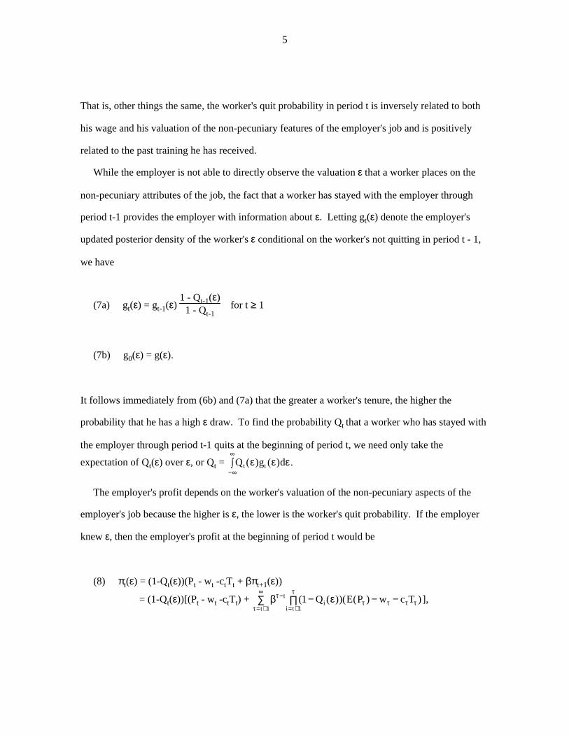
That is, other things the same, the worker's quit probability in period t is inversely related to both

his wage and his valuation of the non-pecuniary features of the employer's job and is positively

related to the past training he has received.

While the employer is not able to directly observe the valuation ε that a worker places on the

non-pecuniary attributes of the job, the fact that a worker has stayed with the employer through

period t-1 provides the employer with information about ε. Letting gt(ε) denote the employer's

updated posterior density of the worker's ε conditional on the worker's not quitting in period t - 1,

we have

(7a) gt(ε) = gt-1(ε) 1 - Qt-1(ε)1 - Qt-1

for t ≥ 1

(7b) g0(ε) = g(ε).

It follows immediately from (6b) and (7a) that the greater a worker's tenure, the higher the

probability that he has a high ε draw. To find the probability Qt that a worker who has stayed with

the employer through period t-1 quits at the beginning of period t, we need only take the

expectation of Qt(ε) over ε, or Qt = Q g dt t−∞

∞

z ( ) ( )ε ε ε.

The employer's profit depends on the worker's valuation of the non-pecuniary aspects of the

employer's job because the higher is ε, the lower is the worker's quit probability. If the employer

knew ε, then the employer's profit at the beginning of period t would be

(8) πt(ε) = (1-Qt(ε))(Pt - wt -ctTt + βπt+1(ε))

= (1-Qt(ε))[(Pt - wt -ctTt) + β ετ τ

ττ τ τ τ

−

= += +

∞−∏∑ − −t

ii tt

Q E P w c T( ( ))( ( ) )111

],

6

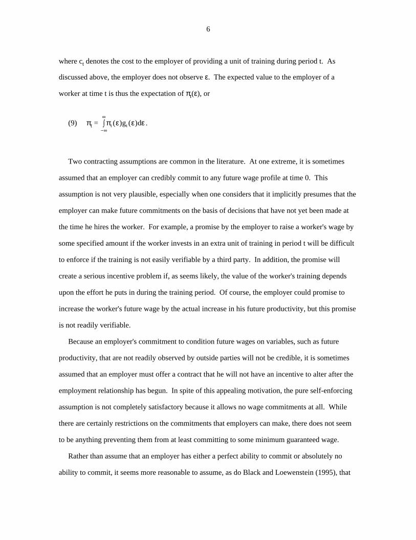
where ct denotes the cost to the employer of providing a unit of training during period t. As

discussed above, the employer does not observe ε. The expected value to the employer of a

worker at time t is thus the expectation of πt(ε), or

(9) πt = π ε ε εt tg d−∞

∞

z ( ) ( ) .

Two contracting assumptions are common in the literature. At one extreme, it is sometimes

assumed that an employer can credibly commit to any future wage profile at time 0. This

assumption is not very plausible, especially when one considers that it implicitly presumes that the

employer can make future commitments on the basis of decisions that have not yet been made at

the time he hires the worker. For example, a promise by the employer to raise a worker's wage by

some specified amount if the worker invests in an extra unit of training in period t will be difficult

to enforce if the training is not easily verifiable by a third party. In addition, the promise will

create a serious incentive problem if, as seems likely, the value of the worker's training depends

upon the effort he puts in during the training period. Of course, the employer could promise to

increase the worker's future wage by the actual increase in his future productivity, but this promise

is not readily verifiable.

Because an employer's commitment to condition future wages on variables, such as future

productivity, that are not readily observed by outside parties will not be credible, it is sometimes

assumed that an employer must offer a contract that he will not have an incentive to alter after the

employment relationship has begun. In spite of this appealing motivation, the pure self-enforcing

assumption is not completely satisfactory because it allows no wage commitments at all. While

there are certainly restrictions on the commitments that employers can make, there does not seem

to be anything preventing them from at least committing to some minimum guaranteed wage.

Rather than assume that an employer has either a perfect ability to commit or absolutely no

ability to commit, it seems more reasonable to assume, as do Black and Loewenstein (1995), that

7

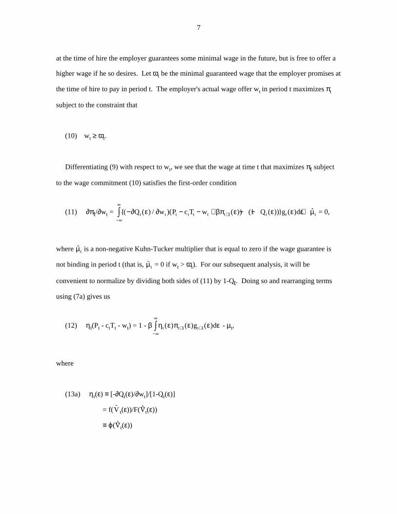
at the time of hire the employer guarantees some minimal wage in the future, but is free to offer a

higher wage if he so desires. Let ωt be the minimal guaranteed wage that the employer promises at

the time of hire to pay in period t. The employer's actual wage offer wt in period t maximizes πt

subject to the constraint that

(10) wt ≥ ωt.

Differentiating (9) with respect to wt, we see that the wage at time t that maximizes πt subject

to the wage commitment (10) satisfies the first-order condition

(11) ∂πt/∂wt = {( ( ) / )( ( )) ( ( ))} ( ) $− − − + − − +−∞

∞

+z ∂ ε ∂ βπ ε ε ε ε µQ w P c T w Q g dt t t t t t t t t t1 1 = 0,

where $µ t is a non-negative Kuhn-Tucker multiplier that is equal to zero if the wage guarantee is

not binding in period t (that is, $µ t = 0 if wt > ωt). For our subsequent analysis, it will be

convenient to normalize by dividing both sides of (11) by 1-Qt. Doing so and rearranging terms

using (7a) gives us

(12) ηt(Pt - ctTt - wt) = 1 - β η ε π ε ε εt t tg d( ) ( ) ( )+−∞

∞

+z 1 1 - µt,

where

(13a) ηt(ε) ≡ [-∂Qt(ε)/∂wt]/[1-Qt(ε)]

= f($V t(ε))/F(V̂t(ε))

≡ ϕ(V̂t(ε))

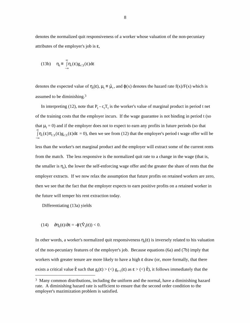
8

denotes the normalized quit responsiveness of a worker whose valuation of the non-pecuniary

attributes of the employer's job is ε,

(13b) ηt ≡ η ε ε εt tg d−∞

∞

+z ( ) ( )1

denotes the expected value of ηt(ε), µt ≡ $µ t , and ϕ(x) denotes the hazard rate f(x)/F(x) which is

assumed to be diminishing.3

In interpreting (12), note that Pt - ctTt is the worker's value of marginal product in period t net

of the training costs that the employer incurs. If the wage guarantee is not binding in period t (so

that µt = 0) and if the employer does not to expect to earn any profits in future periods (so that

η ε π ε ε εt t tg d( ) ( ) ( )+−∞

∞

+z 1 1 = 0), then we see from (12) that the employer's period t wage offer will be

less than the worker's net marginal product and the employer will extract some of the current rents

from the match. The less responsive is the normalized quit rate to a change in the wage (that is,

the smaller is ηt), the lower the self-enforcing wage offer and the greater the share of rents that the

employer extracts. If we now relax the assumption that future profits on retained workers are zero,

then we see that the fact that the employer expects to earn positive profits on a retained worker in

the future will temper his rent extraction today.

Differentiating (13a) yields

(14) ∂ηt(ε)/∂ε = -ϕ'(V̂t(ε)) < 0.

In other words, a worker's normalized quit responsiveness ηt(ε) is inversely related to his valuation

of the non-pecuniary features of the employer's job. Because equations (6a) and (7b) imply that

workers with greater tenure are more likely to have a high ε draw (or, more formally, that there

exists a critical value ε̂ such that gt(ε) > (<) gt+1(ε) as ε > (<) ε̂), it follows immediately that the 3 Many common distributions, including the uniform and the normal, have a diminishing hazardrate. A diminishing hazard rate is sufficient to ensure that the second order condition to theemployer's mazimization problem is satisfied.

9

greater is a worker's tenure t, the lower is his expected quit responsiveness ηt. As discussed

above, a falling ηt provides the employer with an incentive to reduce his wage offer over time.

Thus, if training and productivity growth are not sufficiently high, the self-enforcing wage will fall

with tenure.4 Of course, a sufficiently high rate of productivity growth will cause the self-

enforcing wage to rise, although at a lower rate than productivity.

By offering a wage guarantee at the time the worker is hired, the employer in effect promises to

limit the amount of rents that he will attempt to extract in the future. Because the employer's

future attempts to extract rents lead to quits that are not jointly optimal, it will generally be

efficient to offer a positive wage guarantee. Of course, although a higher wage guarantee has the

advantage of reducing quits, it also induces dismissals when there is a negative value of marginal

product shock vt. As discussed by Black and Loewenstein, the optimal wage guarantee just

balances these two competing considerations.

In our current multiperiod setting, it might be most natural that the wage commitment take the

form of a promise never to cut the wage of any retained worker in the future, so that the guaranteed

wage in period t simply equals the wage offer in the previous period, or ωt = wt-1. Besides being

intuitively plausible, this form of the wage guarantee can be justified on efficiency grounds

because the resulting contract is easy to implement and prevents the employer from making low

future wage offers that induce inefficient turnover. From our discussion above, we know that this

constraint will be binding when training and productivity growth are relatively low. Given

diminishing returns to training (i.e., ψ'' < 0), the wage guarantee will generally be binding once a

worker's tenure becomes sufficiently high.

4 The observant reader may note the presence of an additional effect: a worker with a higher ε ismore valuable to the employer because he has a lower quit rate (in equation (12), this effect works

through the fact that β ( ( ) / ) ( ) ( )η ε η π ε ε εt t t tg d+−∞

∞

+z 1 1 tends to rise over time). This effect in and of

itself would cause the self-enforcing wage to increase, but is generally dominated by the effectfrom the falling ηt. For example, when f(y) and g(ε) are normal densities and β is not extremelyclose to 1, one can show using numerical methods that the self-enforcing wage will fall with tenureif there is no productivity growth over time.

10

We might also note that there are other possible justifications of a wage guarantee besides its

potential use as a means of preventing employers from extracting excessive rents from workers. In

accordance with the suggestion by Shapiro and Stiglitz (1984) and the efficiency wage literature,

the guaranteed wage may be the lowest wage that the employer can offer and still deter workers

from shirking. Alternatively, the constraint may perhaps be justified as representing a "social

norm" that the employer must adhere to if he does not want to hurt the morale of his workers. In

any case, what is crucial for our current analysis is not the exact nature and level of the wage

guarantee, but simply the fact that a wage guarantee exists and may be binding. We have thus

chosen to simplify the ensuing discussion by taking the actual wage guarantee as being determined

exogenously to our model.5

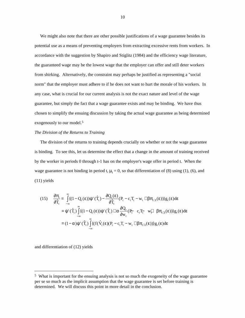
The Division of the Returns to Training

The division of the returns to training depends crucially on whether or not the wage guarantee

is binding. To see this, let us determine the effect that a change in the amount of training received

by the worker in periods 0 through t-1 has on the employer's wage offer in period t. When the

wage guarantee is not binding in period t, µt = 0, so that differentiation of (8) using (1), (6), and

(11) yields

(15) ∂π∂

t

tT$= {( ( )) ' ( $ )

( )$

( ( ))} ( )1 1− − − − +−∞

∞

+z Q TQ

TP c T w g dt t

t

tt t t t t tε ψ ∂ ε

∂βπ ε ε ε

= − + − − +−∞

∞

+zψ ε ψ α ∂∂

βπ ε ε ε' ( $ ) {( ( )) ' ( $ ) ( ( ))} ( )T Q TQ

wP c T w g dt t t

t

tt t t t t t1 1

= − − − +−∞

∞

+z( ) ' ( $ ) {( ( $ ( )( ( ))} ( )1 1α ψ ε βπ ε ε εT f V P c T w g dt t t t t t t t

and differentiation of (12) yields

5 What is important for the ensuing analysis is not so much the exogeneity of the wage guaranteeper se so much as the implicit assumption that the wage guarantee is set before training isdetermined. We will discuss this point in more detail in the conclusion.

11

(16) ∂wt∂T̂t

=

ψ η α φ ε βπ ε ε ε

η φ ε βπ ε ε ε

' ( $ )[ ' ( $ ( ))( ( )) ( ) ]

' ( $ ( ))( ( )) ( ) ]

T V P c T w g d

V P c T w g d

t t t t t t t t t

t t t t t t t t

− − − +

− − − +

+ +−∞

∞

+ +−∞

∞

z

z

1 1

1 1

> 0.

When training is purely specific, α = 0 and equations (15) and (16) reduce to

∂π∂

ψ ε βπ ε ε εt

tt t t t t t t tT

T f V P c T w g d$

' ( $ ) {( ( $ ( )( ( ))} ( )= − − +−∞

∞

+z 1 ,

∂∂wt

t$T

= ψ

η φ ε βπ ε ε ε

' ( $ )

( / ) ' ( $ ( ))( ( )) ( ) ]

T

V P c T w g d

t

t t t t t t t t1 1 1 1− − − + + +−∞

∞

z .

Thus, in periods where the wage guarantee is not binding, the employer shares part, but not all, of

the returns to the past investments in specific training with the worker. Naturally, this implies that

the worker will share the cost of the training investment in the form of a lower wage at the time of

the investment.

In contrast, when α = 1, (15) and (16) reduce to ∂πt/∂T̂t = 0 and ∂wt/∂T̂t = ψ'(T̂t), which is the

standard result that the worker receives all the returns to past investments in general training.

Because a general training investment in period τ does not raise the employer's future profits, the

employer will not be willing to incur any of the costs of general training. Thus, training will occur

only if the worker bears the full cost of training, either directly or indirectly in the form of a lower

wage.

The result that the worker realizes all the returns and incurs the entire cost of general training

depends crucially on the assumption that the employer's promised wage guarantee (10) is never

binding. To see this, note that if the wage guarantee is binding at time t, then the Kuhn-Tucker

multiplier µt is positive and wt = ωt. Differentiation of (11) then yields

12

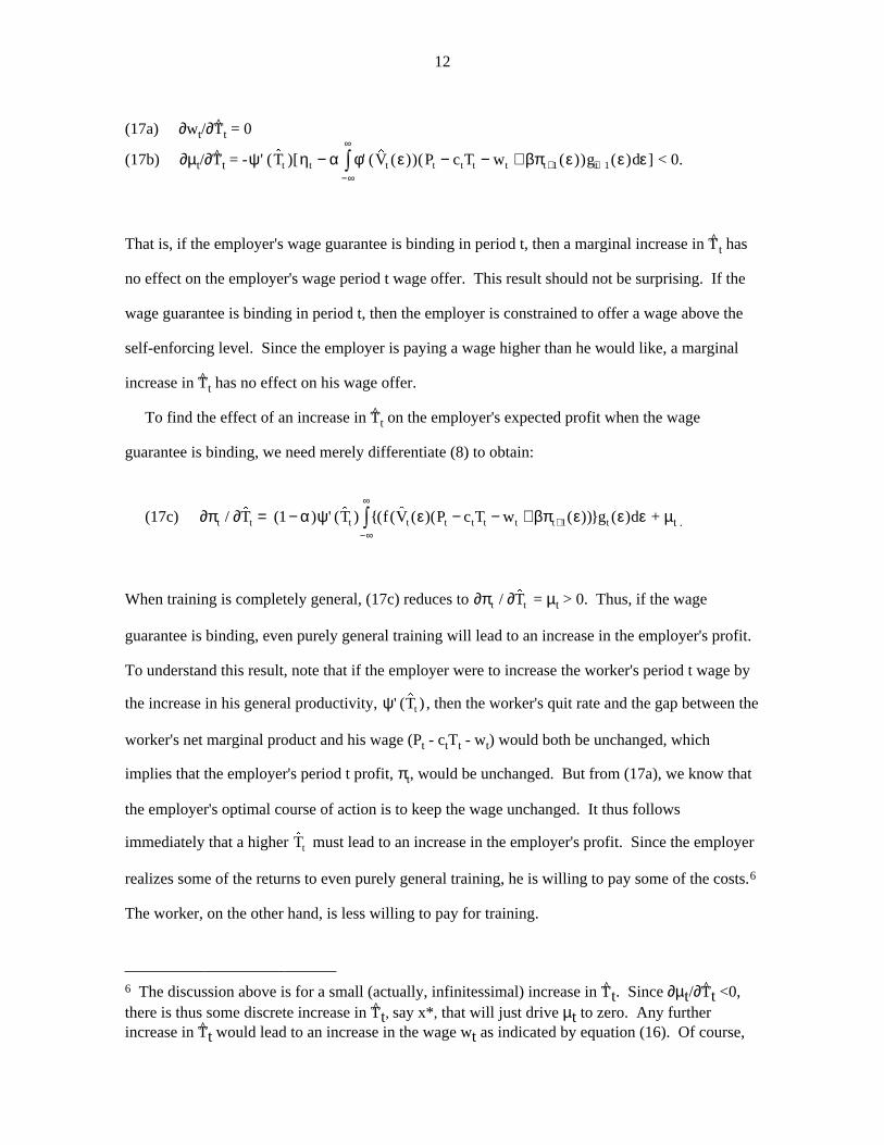
(17a) ∂wt/∂T̂t = 0

(17b) ∂µt/∂T̂t = -ψ η α φ ε βπ ε ε ε' ( $ )[ ' ( $ ( ))( ( )) ( ) ]T V P c T w g dt t t t t t t t t− − − + + +−∞

∞

z 1 1 < 0.

That is, if the employer's wage guarantee is binding in period t, then a marginal increase in T^t has

no effect on the employer's wage period t wage offer. This result should not be surprising. If the

wage guarantee is binding in period t, then the employer is constrained to offer a wage above the

self-enforcing level. Since the employer is paying a wage higher than he would like, a marginal

increase in T^t has no effect on his wage offer.

To find the effect of an increase in T^t on the employer's expected profit when the wage

guarantee is binding, we need merely differentiate (8) to obtain:

(17c) ∂π ∂ α ψ ε βπ ε ε εt t t t t t t t t tT T f V P c T w g d/ $ ( ) ' ( $ ) {( ( $ ( )( ( ))} ( )= − − − +−∞

∞

+z1 1 + µt .

When training is completely general, (17c) reduces to ∂π ∂t tT/ $ = µt > 0. Thus, if the wage

guarantee is binding, even purely general training will lead to an increase in the employer's profit.

To understand this result, note that if the employer were to increase the worker's period t wage by

the increase in his general productivity, ψ' ( $ )Tt , then the worker's quit rate and the gap between the

worker's net marginal product and his wage (Pt - ctTt - wt) would both be unchanged, which

implies that the employer's period t profit, πt, would be unchanged. But from (17a), we know that

the employer's optimal course of action is to keep the wage unchanged. It thus follows

immediately that a higher $Tt must lead to an increase in the employer's profit. Since the employer

realizes some of the returns to even purely general training, he is willing to pay some of the costs.6

The worker, on the other hand, is less willing to pay for training.

6 The discussion above is for a small (actually, infinitessimal) increase in T^t. Since ∂µt/∂T̂t <0,there is thus some discrete increase in T^t, say x*, that will just drive µt to zero. Any furtherincrease in T^t would lead to an increase in the wage wt as indicated by equation (16). Of course,

13

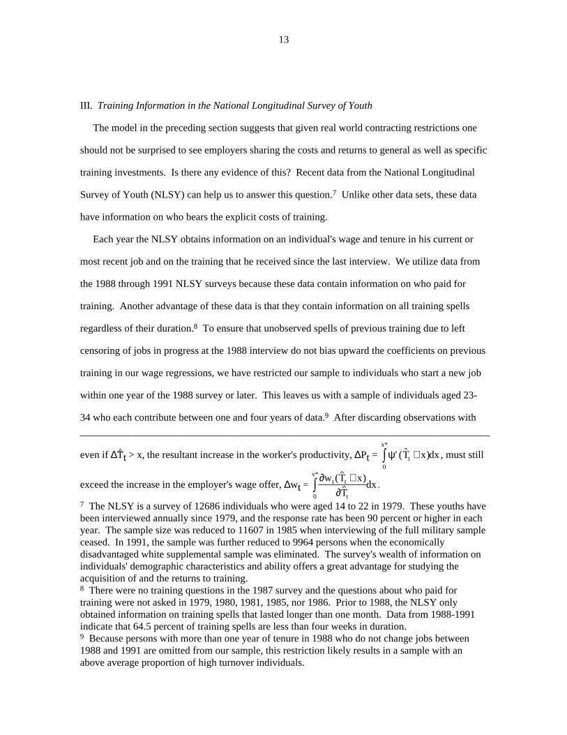
III. Training Information in the National Longitudinal Survey of Youth

The model in the preceding section suggests that given real world contracting restrictions one

should not be surprised to see employers sharing the costs and returns to general as well as specific

training investments. Is there any evidence of this? Recent data from the National Longitudinal

Survey of Youth (NLSY) can help us to answer this question.7 Unlike other data sets, these data

have information on who bears the explicit costs of training.

Each year the NLSY obtains information on an individual's wage and tenure in his current or

most recent job and on the training that he received since the last interview. We utilize data from

the 1988 through 1991 NLSY surveys because these data contain information on who paid for

training. Another advantage of these data is that they contain information on all training spells

regardless of their duration.8 To ensure that unobserved spells of previous training due to left

censoring of jobs in progress at the 1988 interview do not bias upward the coefficients on previous

training in our wage regressions, we have restricted our sample to individuals who start a new job

within one year of the 1988 survey or later. This leaves us with a sample of individuals aged 23-

34 who each contribute between one and four years of data.9 After discarding observations with

even if ∆T̂t > x, the resultant increase in the worker's productivity, ∆Pt = ψ' ( $ )*

T x dxt

x

+z0

, must still

exceed the increase in the employer's wage offer, ∆wt = ∂

∂w T x

Tdxt t

t

x ( $ )$

* +z0

.

7 The NLSY is a survey of 12686 individuals who were aged 14 to 22 in 1979. These youths havebeen interviewed annually since 1979, and the response rate has been 90 percent or higher in eachyear. The sample size was reduced to 11607 in 1985 when interviewing of the full military sampleceased. In 1991, the sample was further reduced to 9964 persons when the economicallydisadvantaged white supplemental sample was eliminated. The survey's wealth of information onindividuals' demographic characteristics and ability offers a great advantage for studying theacquisition of and the returns to training.8 There were no training questions in the 1987 survey and the questions about who paid fortraining were not asked in 1979, 1980, 1981, 1985, nor 1986. Prior to 1988, the NLSY onlyobtained information on training spells that lasted longer than one month. Data from 1988-1991indicate that 64.5 percent of training spells are less than four weeks in duration.9 Because persons with more than one year of tenure in 1988 who do not change jobs between1988 and 1991 are omitted from our sample, this restriction likely results in a sample with anabove average proportion of high turnover individuals.

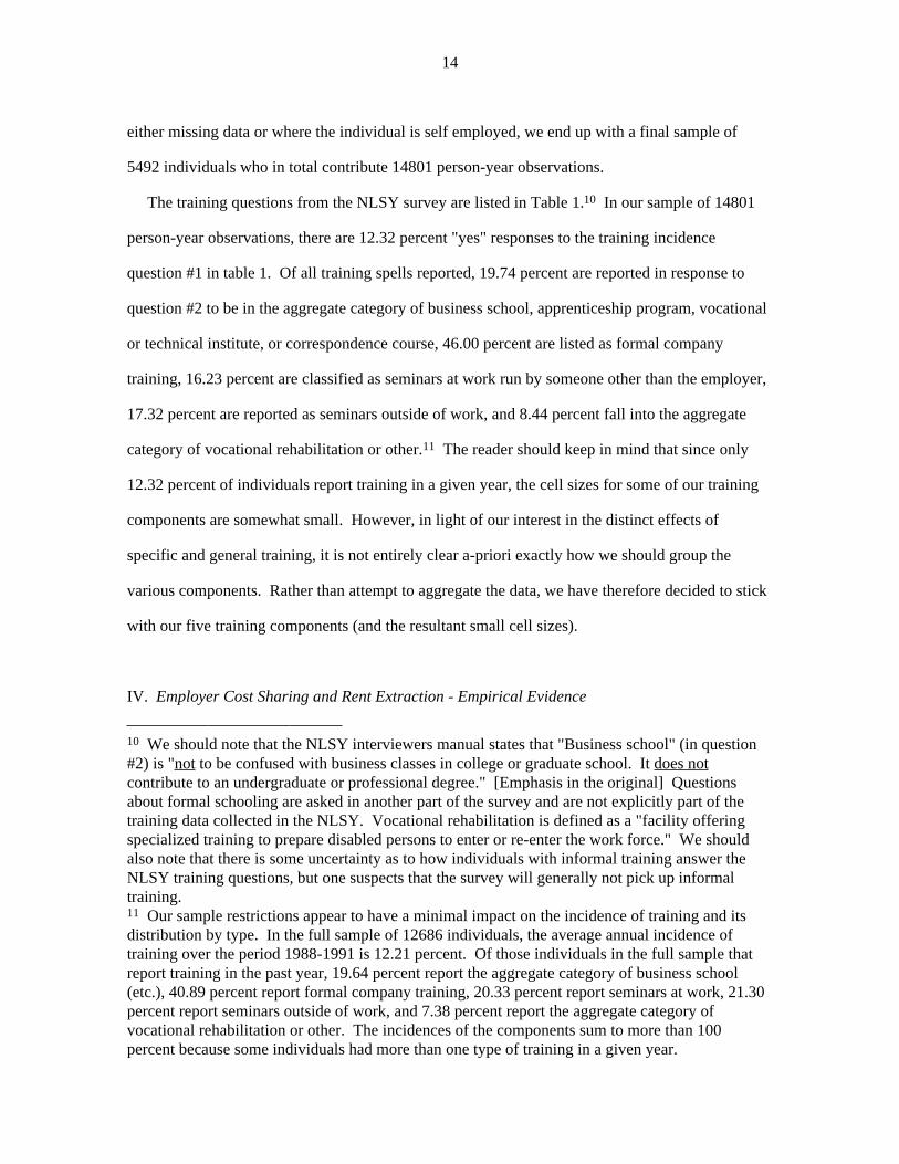
14

either missing data or where the individual is self employed, we end up with a final sample of

5492 individuals who in total contribute 14801 person-year observations.

The training questions from the NLSY survey are listed in Table 1.10 In our sample of 14801

person-year observations, there are 12.32 percent "yes" responses to the training incidence

question #1 in table 1. Of all training spells reported, 19.74 percent are reported in response to

question #2 to be in the aggregate category of business school, apprenticeship program, vocational

or technical institute, or correspondence course, 46.00 percent are listed as formal company

training, 16.23 percent are classified as seminars at work run by someone other than the employer,

17.32 percent are reported as seminars outside of work, and 8.44 percent fall into the aggregate

category of vocational rehabilitation or other.11 The reader should keep in mind that since only

12.32 percent of individuals report training in a given year, the cell sizes for some of our training

components are somewhat small. However, in light of our interest in the distinct effects of

specific and general training, it is not entirely clear a-priori exactly how we should group the

various components. Rather than attempt to aggregate the data, we have therefore decided to stick

with our five training components (and the resultant small cell sizes).

IV. Employer Cost Sharing and Rent Extraction - Empirical Evidence

10 We should note that the NLSY interviewers manual states that "Business school" (in question#2) is "not to be confused with business classes in college or graduate school. It does notcontribute to an undergraduate or professional degree." [Emphasis in the original] Questionsabout formal schooling are asked in another part of the survey and are not explicitly part of thetraining data collected in the NLSY. Vocational rehabilitation is defined as a "facility offeringspecialized training to prepare disabled persons to enter or re-enter the work force." We shouldalso note that there is some uncertainty as to how individuals with informal training answer theNLSY training questions, but one suspects that the survey will generally not pick up informaltraining.11 Our sample restrictions appear to have a minimal impact on the incidence of training and itsdistribution by type. In the full sample of 12686 individuals, the average annual incidence oftraining over the period 1988-1991 is 12.21 percent. Of those individuals in the full sample thatreport training in the past year, 19.64 percent report the aggregate category of business school(etc.), 40.89 percent report formal company training, 20.33 percent report seminars at work, 21.30percent report seminars outside of work, and 7.38 percent report the aggregate category ofvocational rehabilitation or other. The incidences of the components sum to more than 100percent because some individuals had more than one type of training in a given year.

15

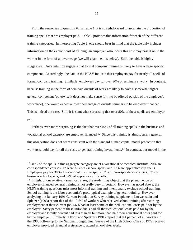
From the responses to question #3 in Table 1, it is straightforward to ascertain the proportion of

training spells that are employer paid. Table 2 provides this information for each of the different

training categories. In interpreting Table 2, one should bear in mind that the table only includes

information on the explicit cost of training; an employer who incurs this cost may pass it on to the

worker in the form of a lower wage (we will examine this below). Still, the table is highly

suggestive. One's intuition suggests that formal company training is likely to have a large specific

component. Accordingly, the data in the NLSY indicate that employers pay for nearly all spells of

formal company training. Similarly, employers pay for over 90% of seminars at work. In contrast,

because training in the form of seminars outside of work are likely to have a somewhat higher

general component (otherwise it does not make sense for it to be offered outside of the employer's

workplace), one would expect a lower percentage of outside seminars to be employer financed.

This is indeed the case. Still, it is somewhat surprising that over 80% of these spells are employer

paid.

Perhaps even more surprising is the fact that over 40% of all training spells in the business and

vocational school category are employer financed.12 Since this training is almost surely general,

this observation does not seem consistent with the standard human capital model prediction that

workers should pay for all the costs to general training investments.13 In contrast, our model in the

12 46% of the spells in this aggregate category are at a vocational or technical institute, 20% arecorrespondence courses, 17% are business school spells, and 17% are apprenticeship spells.Employers pay for 30% of vocational institute spells, 57% of correspondence courses, 37% ofbusiness school spells, and 67% of apprenticeship spells.13 In light of our relatively small cell sizes, the reader may object that the phenomenon ofemployer-financed general training is not really very important. However, as noted above, theNLSY training questions miss most informal training and intentionally exclude school training.School training is the labor economist's prototypical example of general training. However,analyzing the January 1991 Current Population Survey training supplement, Loewenstein andSpletzer (1993) report that of the 13.6% of workers who received school training after startingemployment at their current job, 56% had at least some of their educational costs paid for by theemployer. Sixty percent of these individuals had all their educational costs paid for by theemployer and twenty percent had less than all but more than half their educational costs paid forby the employer. Similarly, Altonji and Spletzer (1991) report that 9.4 percent of all workers inthe 1986 follow-up to the National Longitudinal Survey of the High School Class of 1972 receivedemployer provided financial assistance to attend school after work.

16

previous section suggests that contracting rigidities make it possible for employers to obtain some

of the returns to general training investments, which in turn means that they are willing to incur

some of the costs.

We can use wage regressions to analyze whether employers are able to obtain some of the

returns to general training. The regression equation in column 1 of Table 3 has a worker's log

wage as its dependent variable. As independent variables in the equation, we have included

variables indicating whether the worker has received each of the different types of training in the

current year, whether or not this training is employer financed, and whether or not this training is

completed. Also included are variables indicating whether the worker has received training in

previous years from the current employer and whether the worker has received training in previous

years from a previous employer.

In addition to the various training variables, the regression contains individual and job

characteristics in order to control for the heterogeneity that may exist between those who receive

training and those who do not. Individual characteristics include not only the worker's age, sex,

race, education, job tenure, and labor market experience, but also his score on the armed forces

qualifying test (which serves an indicator of the worker's ability). Job characteristics include

industry and occupation, whether the worker is in a union, whether the worker's job is part-time,

the size of the employer's establishment, and whether the employer has more than one

establishment.

As expected, the wage regression in column 1 of Table 3 indicates that there is a positive wage

return to completed spells of employer financed training. Nearly all the coefficients on completed

spells of employer financed training are positive and quite a few of these coefficients are

significantly different from zero. In contrast to employer financed training, completed spells of

most types of non-employer financed training [not reported in the table] do not yield a positive

wage return. One possible explanation for this is that individual workers are not particularly adept

on their own in choosing training activities that have a high positive return. Another possible

explanation is that individuals answering the survey may be misreporting some primarily self-

17

financed leisure time activities as training. At any rate, the rest of our discussion will focus on

employer financed training, which is more germane given our current concerns.14

As discussed above, the NLSY data indicate that besides nearly always bearing the explicit

costs of specific training, employers also frequently incur the explicit costs of what appears to be

general training. The question that naturally arises is whether these costs are partially passed on to

workers in the form of lower wages during the training period. Interestingly, the wage regression

in column 1 of Table 3 does not provide much evidence of this. The coefficients labeled "marginal

effects of uncompleted spells" indicate the differential wage returns between uncompleted and

completed spells of employer financed training in the current year. As expected, most of these

coefficients are negative, and the ones that are positive are small in magnitude. However, none of

the coefficients are statistically different from zero. The returns to uncompleted spells of training

(as compared to no training) can be obtained by adding the returns to completed spells of training

to the marginal effects of uncompleted spells. While the estimated returns to uncompleted spells

of formal company training and outside seminars are negative, these estimated returns are both

statistically insignificant and economically small (-.014 and -.012). Of course, our finding that

uncompleted spells of training do not have a negative effect on wages should be viewed with some

caution since the number of uncompleted training spells in our sample is quite small. However, as

alluded to in the introduction, a host of other studies have obtained the same result.15

14 We also will not have anything to say about "other training" except to note that analysis of"other training" responses in the full sample 1993 Computer Assisted Personal Interview revealsthat this training variable is quite a hodgepodge. Four of the individuals responding "other" in1993 indicated that they had received informal on the job training, 14 indicated that they received"on the job training", 14 indicated that they attended seminars or vocational-technical programs(training which should have been placed in a preceding category), 22 indicated that they receivedsome form of schooling such as adult education or classroom training, 17 indicated some form ofgovernment training, 10 indicated that training occurred in prison, and 40 responses could not beclassified.15 We might note that the NLSY does not provide information on a worker's wage at the beginningof a training period. It is possible that training lowers a worker's wage at the beginning of thetraining period, but that the wage is increased through the training period as a worker becomesmore productive. However, Barron, Black, and Loewenstein (1989) find that the amount of on-the-job training in the first three months has no statistically significant effect on the starting wage.And Barron, Berger, and Black's (1993) results indicate that the estimated effect of training on the

18

Employers should only be willing to pay the costs of training if they are able to realize some of

the returns. Is there any evidence to suggest that employers extract any of the returns to general

training? While the costs of a training spell occur contemporaneously, the returns occur in the

future. To determine the worker's return to training, we thus look at the effect of completed spells

of past training on the current wage. While we do not have a direct measure of the employer's

return, we can make some inferences about employers' rent extraction by comparing the wage

return to training when a worker remains at the employer providing the training with the return

when he moves to a new employer.

When one examines the returns to employer financed training, one sees that the coefficient on

previous spells of formal company training at the current employer is .0654, but the coefficient on

previous spells of formal company training at a previous employer is only .0087. Thus, while a

spell of employer financed formal company training in a previous year has a positive and

significant effect on a worker's current wage if the worker obtained the training at his current

employer, it has essentially no effect on his wage if it was obtained at a previous employer. This is

consistent with our hypothesis that formal company training is primarily specific. By way of

contrast, the coefficient on business or vocational school training at a previous employer is .1410

and significantly different from zero, which is consistent with the fact that a substantial component

of this training is likely to be general. Similarly, the statistically significant positive coefficients

on outside and inside seminars at a previous employer (the coefficients are .2599, and .0802,

respectively) suggest that a substantial part of this training is general as well.

Unlike business and vocational school training at a previous employer, previous employer

financed training in business and vocational schools at the current employer does not appear to

starting wage may be somewhat sensitive to the exact specification of the starting wage equation,but if it is negative, it is certainly very small. Barron, Black, and Loewenstein suggest that theirinability to obtain compensating differentials may stem in part from unmeasured differences inworker ability. This is less of a problem in the National Longitudinal Survey of Youth, whichcontains richer individual data. Using the NLSY data through 1983, Lynch (1992) also fails toobtain a significant negative effect of uncompleted training on the wage. And using NLSY datafrom 1979 to 1982, Parsons (1989) does not find any evidence of a compensating differential forjobs with greater learning opportunities.

19

have a positive effect on the current wage (the coefficient is an insignificant -.0673). A similar

result holds for outside and, to a lesser extent, inside seminars: while previous employer financed

outside seminars at the current employer have a significantly positive effect on the current log

wage, the returns (.1463) are smaller than those associated with employer financed outside

seminars while at a previous employer. This result is consistent with our hypothesis that

employers extract some of the return to general training.

The coefficients in column 1 of table 3 indicate that the differential return between employer

financed formal company training at a previous and current employer is -.057, which is statistically

different from zero at the 10% confidence level. For inside and outside seminars, the differential

returns are .049 and .114, respectively. And the differential return for business and vocational

school is .208, which is statistically different from zero at the 5% confidence level. These

estimated differential returns are listed in table 4. As one would expect, the difference between

the return to training at a previous and current employer is smaller the more specific is the training.

However, it is difficult for the conventional model to explain the large positive differential for

general training. Indeed, the only convincing explanation we can find is that employers are

extracting some of the returns to general training.

At first glance, one might suspect that the estimated positive differential for general training

might be due to a bias introduced by individuals' endogenous separation decisions. It is indeed

true that the returns to previous training at previous employers are estimated from the sample of

individuals who switch jobs. Because persons switch jobs when they find an alternative that is

more attractive than their previous job, our estimated returns to training in previous jobs may

overstate the return that a worker who does not switch jobs can expect. However, we should

expect a similar bias in the estimated returns to previous training at the current employer because

these returns are estimated from the sample of individuals who do not switch jobs and these

individuals will on average be in an unusually good job match. In short, our estimated returns to

previous training at the current employer and previous training at past employers are both

20

confounded by individuals' endogenous separation decisions, but there is no reason a priori to

expect the estimated differential to be biased in any particular direction.

As initially pointed out by Barron, Black, and Loewenstein (1989), individuals who are more

able may be more likely to receive training. While our regression equation includes a host of

individual and job characteristics in an attempt to control for heterogeneity that may exist between

those who receive training and those who do not, it is still possible that the training coefficients

may be biased upward because of unmeasured heterogeneity. Although it is difficult to imagine

how this would bias the differential return between training at a current and previous employer, we

can provide an additional check on our results by estimating a fixed effects wage equation.

While a fixed effects wage equation will obviously eliminate any bias introduced by

unobserved personal characteristics, it is not so apparent how a fixed effects equation controls for

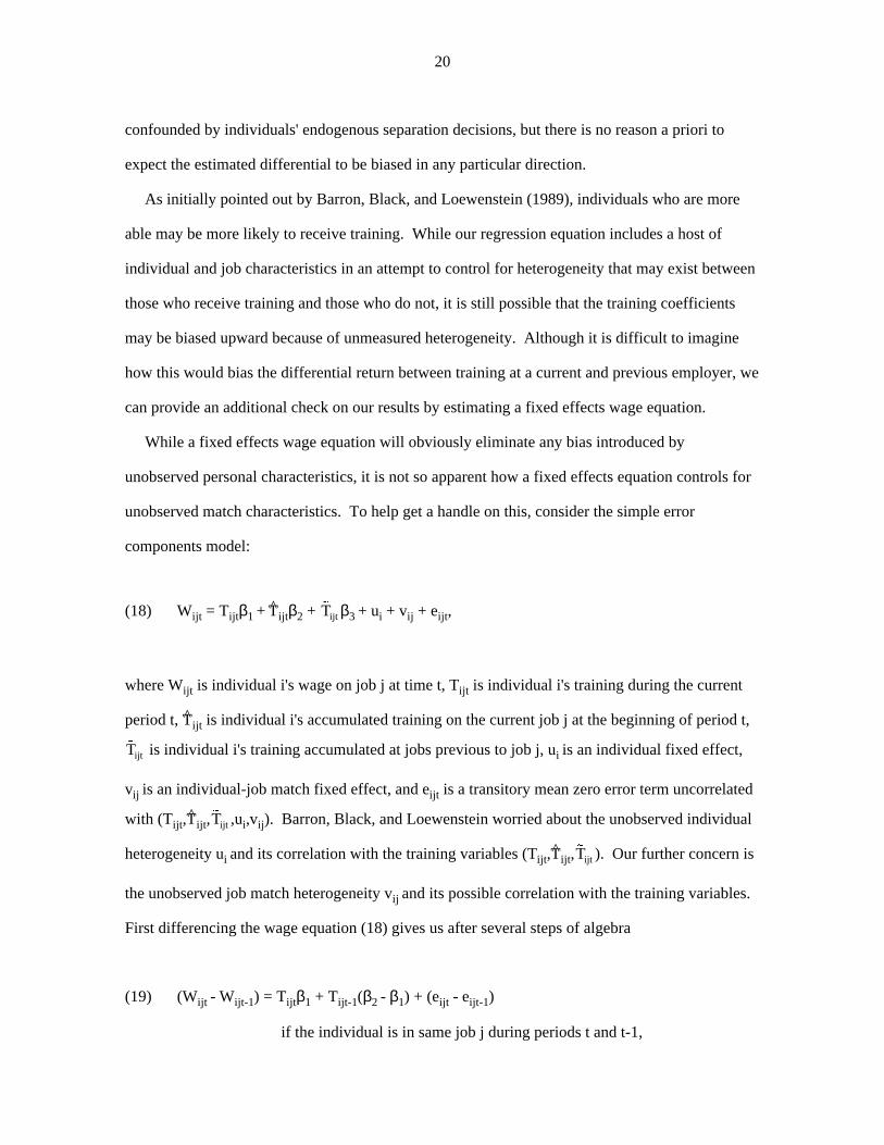
unobserved match characteristics. To help get a handle on this, consider the simple error

components model:

(18) Wijt = Tijtβ1 + T̂ijtβ2 + %Tijt β3 + ui + vij + eijt ,

where Wijt is individual i's wage on job j at time t, Tijt is individual i's training during the current

period t, T̂ijt is individual i's accumulated training on the current job j at the beginning of period t,

%Tijt is individual i's training accumulated at jobs previous to job j, ui is an individual fixed effect,

vij is an individual-job match fixed effect, and eijt is a transitory mean zero error term uncorrelated

with (Tijt ,T̂ijt , %Tijt ,ui,vij). Barron, Black, and Loewenstein worried about the unobserved individual

heterogeneity ui and its correlation with the training variables (Tijt ,T̂ijt , %Tijt ). Our further concern is

the unobserved job match heterogeneity vij and its possible correlation with the training variables.

First differencing the wage equation (18) gives us after several steps of algebra

(19) (Wijt - Wijt-1) = Tijtβ1 + Tijt-1(β2 - β1) + (eijt - eijt-1)

if the individual is in same job j during periods t and t-1,

21

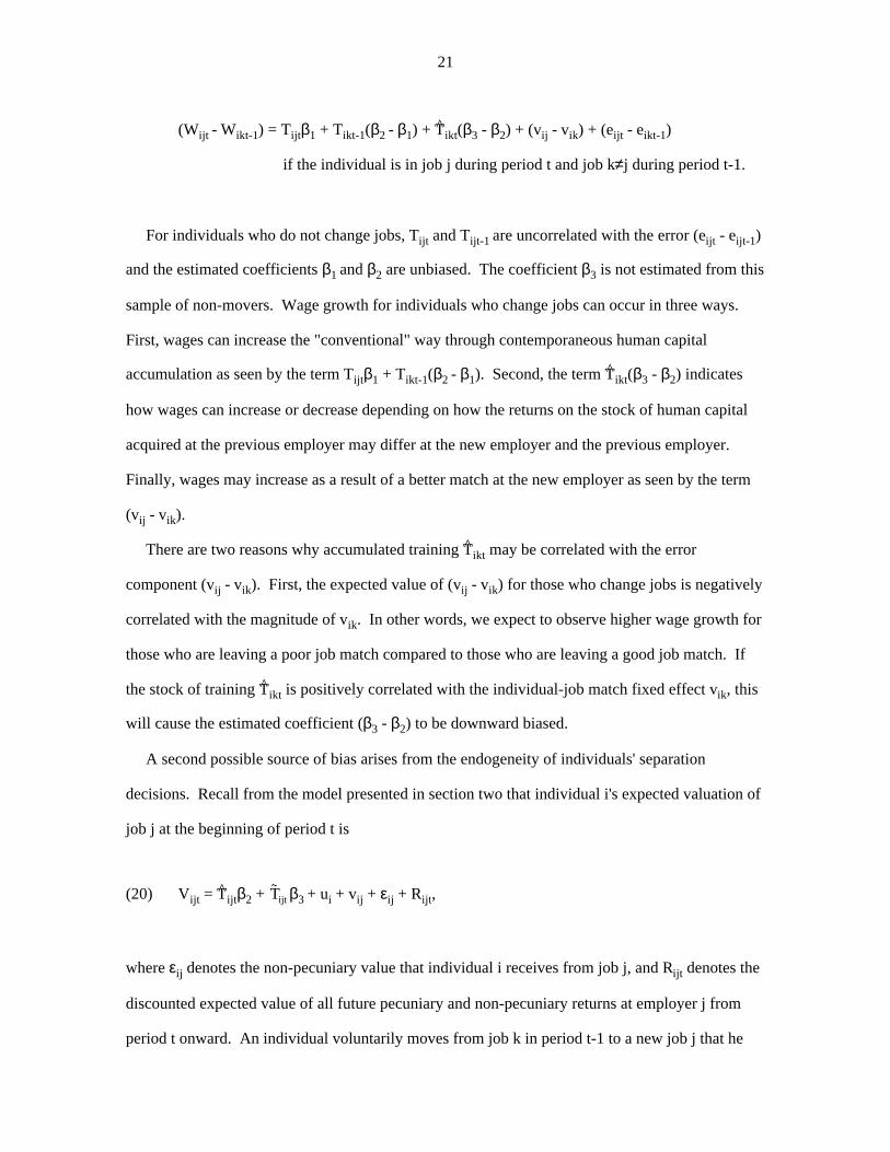
(Wijt - Wikt-1) = Tijtβ1 + Tikt-1(β2 - β1) + T̂ikt(β3 - β2) + (vij - vik) + (eijt - eikt-1)

if the individual is in job j during period t and job k≠j during period t-1.

For individuals who do not change jobs, Tijt and Tijt-1 are uncorrelated with the error (eijt - eijt-1)

and the estimated coefficients β1 and β2 are unbiased. The coefficient β3 is not estimated from this

sample of non-movers. Wage growth for individuals who change jobs can occur in three ways.

First, wages can increase the "conventional" way through contemporaneous human capital

accumulation as seen by the term Tijtβ1 + Tikt-1(β2 - β1). Second, the term T^ikt(β3 - β2) indicates

how wages can increase or decrease depending on how the returns on the stock of human capital

acquired at the previous employer may differ at the new employer and the previous employer.

Finally, wages may increase as a result of a better match at the new employer as seen by the term

(vij - vik).

There are two reasons why accumulated training T^ikt may be correlated with the error

component (vij - vik). First, the expected value of (vij - vik) for those who change jobs is negatively

correlated with the magnitude of vik. In other words, we expect to observe higher wage growth for

those who are leaving a poor job match compared to those who are leaving a good job match. If

the stock of training T^ikt is positively correlated with the individual-job match fixed effect vik, this

will cause the estimated coefficient (β3 - β2) to be downward biased.

A second possible source of bias arises from the endogeneity of individuals' separation

decisions. Recall from the model presented in section two that individual i's expected valuation of

job j at the beginning of period t is

(20) Vijt = T̂ijtβ2 + %Tijt β3 + ui + vij + εij + Rijt ,

where εij denotes the non-pecuniary value that individual i receives from job j, and Rijt denotes the

discounted expected value of all future pecuniary and non-pecuniary returns at employer j from

period t onward. An individual voluntarily moves from job k in period t-1 to a new job j that he

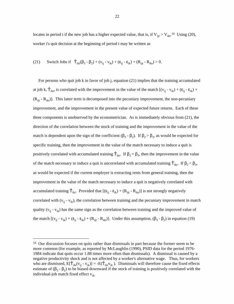
22

locates in period t if the new job has a higher expected value, that is, if Vijt > Vikt.16 Using (20),

worker i's quit decision at the beginning of period t may be written as

(21) Switch Jobs if T^ikt(β3 - β2) + (vij - vik) + (εij - εik) + (Rijt - Rikt) > 0.

For persons who quit job k in favor of job j, equation (21) implies that the training accumulated

at job k, T̂ikt, is correlated with the improvement in the value of the match [(vij - vik) + (εij - εik) +

(Rijt - Rikt)]. This latter term is decomposed into the pecuniary improvement, the non-pecuniary

improvement, and the improvement in the present value of expected future returns. Each of these

three components is unobserved by the econometrician. As is immediately obvious from (21), the

direction of the correlation between the stock of training and the improvement in the value of the

match is dependent upon the sign of the coefficient (β3 - β2). If β2 > β3, as would be expected for

specific training, then the improvement in the value of the match necessary to induce a quit is

positively correlated with accumulated training T^ikt. If β2 = β3, then the improvement in the value

of the match necessary to induce a quit is uncorrelated with accumulated training T^ikt. If β2 < β3,

as would be expected if the current employer is extracting rents from general training, then the

improvement in the value of the match necessary to induce a quit is negatively correlated with

accumulated training T^ikt. Provided that [(εij - εik) + (Rijt - Rikt)] is not strongly negatively

correlated with (vij - vik), the correlation between training and the pecuniary improvement in match

quality (vij - vik) has the same sign as the correlation between training and the improved value of

the match [(vij - vik) + (εij - εik) + (Rijt - Rikt)]. Under this assumption, (β3 - β2) in equation (19)

16 Our discussion focuses on quits rather than dismissals in part because the former seem to bemore common (for example, as reported by McLaughlin (1990), PSID data for the period 1976-1984 indicate that quits occur 1.88 times more often than dismissals). A dismissal is caused by anegative productivity shock and is not affected by a worker's alternative wage. Thus, for workerswho are dismissed, E[T^

ikt(vij - vik)] = -E(T̂iktvik ). Dismissals will therefore cause the fixed effectsestimate of (β3 - β2) to be biased downward if the stock of training is positively correlated with theindividual-job match fixed effect vik.

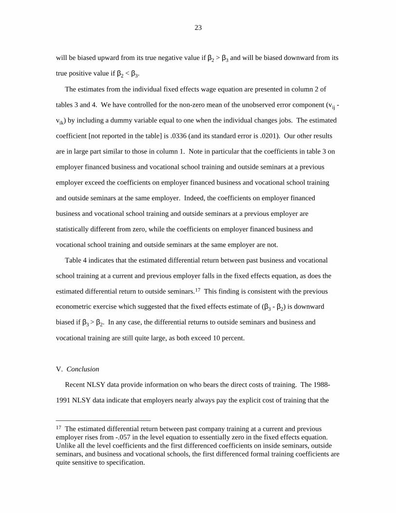
23

will be biased upward from its true negative value if β2 > β3 and will be biased downward from its

true positive value if β2 < β3.

The estimates from the individual fixed effects wage equation are presented in column 2 of

tables 3 and 4. We have controlled for the non-zero mean of the unobserved error component (vij -

vik) by including a dummy variable equal to one when the individual changes jobs. The estimated

coefficient [not reported in the table] is .0336 (and its standard error is .0201). Our other results

are in large part similar to those in column 1. Note in particular that the coefficients in table 3 on

employer financed business and vocational school training and outside seminars at a previous

employer exceed the coefficients on employer financed business and vocational school training

and outside seminars at the same employer. Indeed, the coefficients on employer financed

business and vocational school training and outside seminars at a previous employer are

statistically different from zero, while the coefficients on employer financed business and

vocational school training and outside seminars at the same employer are not.

Table 4 indicates that the estimated differential return between past business and vocational

school training at a current and previous employer falls in the fixed effects equation, as does the

estimated differential return to outside seminars.17 This finding is consistent with the previous

econometric exercise which suggested that the fixed effects estimate of (β3 - β2) is downward

biased if β3 > β2. In any case, the differential returns to outside seminars and business and

vocational training are still quite large, as both exceed 10 percent.

V. Conclusion

Recent NLSY data provide information on who bears the direct costs of training. The 1988-

1991 NLSY data indicate that employers nearly always pay the explicit cost of training that the

17 The estimated differential return between past company training at a current and previousemployer rises from -.057 in the level equation to essentially zero in the fixed effects equation.Unlike all the level coefficients and the first differenced coefficients on inside seminars, outsideseminars, and business and vocational schools, the first differenced formal training coefficients arequite sensitive to specification.

24

worker receives on the employer's premises. Even more strikingly, the employer often pays for the

explicit costs of what appears to be general training: seminars or training programs outside of work

and training that a worker receives in business school, an apprenticeship program, a vocational or

technical institute, or a correspondence course. Evidence from at least two other data sets also

indicates that employers pay for general training, an observation that is contrary to the

conventional human capital model.

We have argued that employers pay for general training because they are able to obtain some of

the returns. This hypothesis is supported by our wage regressions which indicate that completed

spells of general training paid for by previous employers have a larger effect on the wage than

completed spells of general training paid for by the current employer. Given the small cell sizes of

our five training components, the evidence is not entirely conclusive. Although we could have

reduced the variances of our parameter estimates by aggregating the data, we were unsure of the

appropriate way to aggregate. We chose to work with the disaggregated training components in

order to minimize possible differences in specificity within a given category of training.18

Worker mobility costs are an important feature of the theoretical model that we presented in

Section II. As suggested by Bishop (1988) and Parsons (1990), a liquidity constraint facing

workers is another factor that may affect the division of the returns and costs to training.

However, we may note that mobility costs and a high worker discount rate are not sufficient to

induce employers to incur any of the costs of general training. Employers will be willing to incur

some of the costs of general training only if they realize some of the returns. But in the absence of

a binding wage guarantee, the first-order condition for the employer's post-training wage offer

already takes mobility costs and discount factors into account and thus implies that all the returns

18 General training spells are likely both to have a higher wage return than specific training spellsand to be associated with higher subsequent turnover. Thus, including specific and generaltraining spells in the same training category could by itself cause us to estimate a higher wagereturn for training received at a previous employer than for training received at a curent employer.For this reason, we have attempted to ensure that our general training categories really includeonly general training. (For example, it is hard to imagine how business school training couldpossibly be specific).

25

to general human capital will be passed on to workers in the form of higher future wages. This

result is quite robust and holds in both the full commitment and the self-enforcing model. The

prediction that employers pay for all general training is also not affected by tax considerations. If

employers are better able than workers to write off the costs of general training investments, then

we should see employers bearing the explicit costs of training and passing these costs entirely onto

workers in the form of lower wages during the training period; workers should still receive all the

returns to general training. However, as is the case with other data sets, there is no evidence in the

NLSY that workers bear the costs of training in the form of a lower wage.19

One can obtain the prediction that employers share in the returns and costs to general training

investments only by expanding on the set of contracts that employers are allowed to offer.20 Two

contracting assumptions are common in the literature. At one extreme, it is often assumed that an

employer can credibly commit to any future wage profile and at the other extreme, it is sometimes

assumed that an employer must offer a contract that he will not have an incentive to alter after the

employment relationship has begun. We find it more reasonable to assume that at the time of hire

the employer guarantees some minimal future wage (or rate of wage growth), but is free to offer a

higher wage if he so desires. The future wage guarantee serves the purpose of assuring a newly

hired worker that the employer will not extract excessive rents from him should it turn out that he

places a relatively high valuation on the employer's job. When the wage guarantee is binding, an

increase in the worker's productivity caused by an increase in his stock of human capital will not

cause the employer to pay a higher wage. The employer will thus share in the returns to general as

well as specific training.

19 In the self-enforcing model, the result that workers realize all the returns to general training isalso not affected by a legal minimum wage during the training period. In any case, most of theworkers in our sample earn a starting wage that exceeds the legal minimum wage.20 Katz and Ziderman (1990) argue that an employer can realize some of the return to a generaltraining investment if competing firms have imperfect information about generality of thisinvestment and Pichler (1993) points out that a worker will stay with a firm paying a wage belowhis alternative if the prospect of future wage growth from continued general training outweighs theshort-run gain from quitting.

26

Our analysis implicitly assumes that the wage guarantee is set before training is determined. If

training is entirely determined before the wage guarantee is set, then this information will be

incorporated in the optimal wage guarantee; as discussed above, this would likely result in workers

realizing all the returns to general training. The justification for our assumption that training is not

known with certainty before the wage guarantee is set is that the returns and costs to training

investments vary among workers. If information about the returns and costs to training a worker

comes out belatedly over time, some training decisions will likely be postponed until after the

match has started. As we discuss in a recent paper (Loewenstein and Spletzer (1995)), this

hypothesis is supported by the NLSY data. Analysis of the data indicates that a substantial amount

of training is belated.

Besides its potential use as a means of preventing employers from extracting excessive rents

from workers, there are other possible reasons for a future wage guarantee. In accordance with the

efficiency wage literature, a wage guarantee might arise from employers' efforts to deter shirking

by workers. Alternatively, the constraint may reflect a "social norm" that the employer must

adhere to if he does not want to hurt the morale of his workers. No matter what its cause, a

binding wage guarantee breaks the link between a worker's future productivity and wage rate,

which in turn implies that employers will extract some of the returns to general training.

27

References

Altonji, Joseph G. and James R. Spletzer. 1991. "Worker Characteristics, Job Characteristics, and the Receipt of On-the-Job Training." Industrial and Labor Relations Review, pp. 58-79.

Barron, John M., Mark C. Berger, and Dan A. Black. 1993. "Do Workers Pay for On-the-Job Training?" University of Kentucky Working Paper #E-169-93.

Barron, John M., Dan A. Black, and Mark A. Loewenstein. 1989. "Job Matching and On-the- Job Training." Journal of Labor Economics, pp. 1-19.

Becker, Gary S. 1962. "Investment in Human Capital: A Theoretical Analysis." Journal of Political Economy, pp. 9-49.

Bishop, John. 1988. "Do Employers Share the Costs and Benefits of General Training?" Mimeo, Center for Advanced Human Resource Studies, Cornell University.

Black, Dan A. and Mark A. Loewenstein. 1995. "Dismissals and Match-Specific Rents." Bureau of Labor Statistics Working Paper #247 (revised).

Hashimoto, Masanori. 1981. "Firm-Specific Investment as a Shared Investment." American Economic Review, pp. 475-482.

Johnson, William R. 1978 "A Theory of Job Shopping." Quarterly Journal of Economics, pp. 261-78.

Kuhn, Peter. 1994. "Demographic Groups and Personnel Policy." Labour Economics, pp. 49-70.

Katz, Eliakim and Adrian Ziderman. 1990. "Investment in General Training: The Role of Information and Labour Mobility." The Economic Journal, pp. 1147-58.

Loewenstein, Mark A. and James R. Spletzer. 1993. "Training, Tenure, and Cost-Sharing: Evidence from the CPS." Unpublished paper presented at the 1993 Western Economic Meetings.

Loewenstein, Mark A. and James R. Spletzer. 1995. "Belated Training: The Relationship Between Training, Tenure, and Wages." Unpublished paper, Bureau of Labor Statistics.

Lynch, Lisa M. 1992. "Private Sector Training and the Earnings of Young Workers." American Economic Review, pp. 299-312.

McLaughlin, Kenneth J. 1990. "General Productivity in a Theory of Quits and Layoffs." Journal of Labor Economics, pp. 75-98.

Parsons, Donald O. 1989. "On-the-Job Learning and Wage Growth." Mimeo, Ohio State University.

Parsons, Donald O. 1990. "The Firm's Decision to Train." Research in Labor Economics, pp. 53-75.

28

Pichler, Eva. 1993. "Cost-sharing of General and Specific Training with Depreciation of Human Capital." Economics of Education Review, pp. 117-24.

Shapiro, Carl and Joseph E. Stiglitz. 1984. "Equilibrium Unemployment as a Worker Discipline Device." American Economic Review, pp. 433-44.

Table 1: NLSY Training Questions_ _1) Since [date of the last interview], did you attend any training program or any on-the-job training designed to help people find a job, improve job skills, or learn a new job?2) Which category best describes where you received this training?

Business schoolApprenticeship programA vocational or technical instituteA correspondence courseFormal company training run by employer or military trainingSeminars or training programs at work run by someone other

than employerSeminars or training programs outside of workVocational rehabilitation centerOther (specify)

3) Who paid for this training program? [Check all that apply]Self or familyEmployerJob Training Partnership ActTrade Adjustment ActJob Corps ProgramWork Incentive ProgramVeteran's AdministrationVocational RehabilitationOther (specify)

_ _

Table 2: The Probability that a Training Spell is Employer Paid

Type of Training Percentage of Spellsthat are Employer Paid

Formal Company Training 95.71%Seminars at Work 91.22%Seminars Outside of Work 81.96%Business School, Vocational Institute, etc. 42.22%Other 45.45%

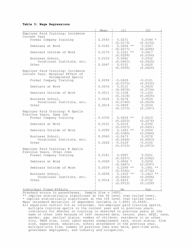
Table 3: Wage Regressions

| Mean | (1) (2) |Employer Paid Training: Incidence | | |Current Year | | | Formal Company Training | 0.0543 | 0.0271 0.0346 * | | | (0.0173) (0.0193) | Seminars at Work | 0.0182 | 0.0656 ** 0.0367 | | | (0.0277) (0.0286) | Seminars Outside of Work | 0.0175 | 0.1221 ** 0.0417 | | | (0.0289) (0.0304) | Business School, | 0.0103 | 0.0081 0.0532 | Vocational Institute, etc. | | (0.0401) (0.0424) | Other | 0.0047 | 0.0151 0.0620 | | | (0.0595) (0.0620) |Employer Paid Training: Incidence | | |Current Year, Marginal Effect of | | | Uncompleted Spells | | | Formal Company Training | 0.0094 | -0.0409 -0.0101 | | | (0.0372) (0.0332) | Seminars at Work | 0.0016 | 0.0131 0.0624 | | | (0.0874) (0.0734) | Seminars Outside of Work | 0.0011 | -0.1338 -0.1324 | | | (0.1018) (0.0835) | Business School, | 0.0026 | 0.0274 0.0524 | Vocational Institute, etc. | | (0.0740) (0.0639) | Other | 0.0014 | -0.0849 0.0224 | | | (0.1073) (0.1067) |Employer Paid Training: # Spells | | |Previous Years, Same Job | | | Formal Company Training | 0.0330 | 0.0654 ** 0.0419 | | | (0.0203) (0.0276) | Seminars at Work | 0.0101 | 0.0316 0.0350 | | | (0.0357) (0.0451) | Seminars Outside of Work | 0.0090 | 0.1463 ** 0.0454 | | | (0.0380) (0.0484) | Business School, | 0.0060 | -0.0673 0.0278 | Vocational Institute, etc. | | (0.0446) (0.0603) | Other | 0.0028 | -0.0129 -0.0150 | | | (0.0723) (0.0973) |Employer Paid Training: # Spells | | |Previous Years, Other Jobs | | | Formal Company Training | 0.0181 | 0.0087 0.0521 | | | (0.0257) (0.0342) | Seminars at Work | 0.0049 | 0.0802 * 0.0256 | | | (0.0487) (0.0597) | Seminars Outside of Work | 0.0039 | 0.2599 ** 0.1481 ** | | | (0.0562) (0.0736) | Business School, | 0.0058 | 0.1410 ** 0.1423 ** | Vocational Institute, etc. | | (0.0463) (0.0694) | Other | 0.0014 | -0.0433 -0.0732 | | | (0.0912) (0.1228) | | | |Individual Fixed Effects | | No Yes |Standard errors in parentheses. Sample Size = 14801.** implies statistically significant at the 5% level (two tailed test).* implies statistically significant at the 10% level (two tailed test).Mean (standard deviation) of dependent variable is 1.8851 (0.4945).All equations control for an intercept, non-employer paid training spells, multiple training spells in the current year and in previous years, indicators for whether no training is observed in previous years at the same or other jobs because of left censored data, tenure, year, AFQT, race, gender, age, marital status, number of children, residence in an urban city, SMSA size, local labor market unemployment rate, union status, firm size, experience, education, school attendance in the previous year, multiple-site firm, number of previous jobs ever held, part-time work, government employment, and industry and occupation.

Table 4: Differential Returns to Training at Current and Previous Employers (Calculated from Coefficients in Table 3)

| (1) (2) |Employer Paid Training | |Previous Years, Other Jobs - Same Job | | Formal Company Training | -0.0566 * 0.0102 | | (0.0325) (0.0338) | Seminars at Work | 0.0486 -0.0094 | | (0.0602) (0.0599) | Seminars Outside of Work | 0.1136 * 0.1027 | | (0.0688) (0.0783) | Business School, | 0.2083 ** 0.1145 * | Vocational Institute, etc. | (0.0637) (0.0688) | Other | -0.0304 -0.0581 | | (0.1133) (0.1273) | | |Individual Fixed Effects | No Yes |See notes to table 3.