John R. SpletzerCamillo J. TaylorGRASP LaboratoryUniversity of PennsylvaniaPhiladelphia, PA 19104, USAspletzer@grasp.cis.upenn.educjtaylor@grasp.cis.upenn.edu

Dynamic SensorPlanning and Controlfor Optimally TrackingTargets

Abstract

In this paper, we present an approach to the problem of actively con-trolling the configuration of a team of mobile agents equipped withcameras so as to optimize the quality of the estimates derived fromtheir measurements. The issue of optimizing the robots’ configura-tion is particularly important in the context of teams equipped withvision sensors, since most estimation schemes of interest will involvesome form of triangulation.

We provide a theoretical framework for tackling the sensor plan-ning problem, and a practical computational strategy inspired bywork on particle filtering for implementing the approach. We thenextend our framework by showing how modeled system dynamicsand configuration space obstacles can be handled. These ideas havebeen applied to a target tracking task, and demonstrated both insimulation and with actual robot platforms. The results indicate thatthe framework is able to solve fairly difficult sensor planning prob-lems online without requiring excessive amounts of computationalresources.

KEY WORDS—optimal target tracking, sensor fusion, par-ticle filtering

1. Introduction

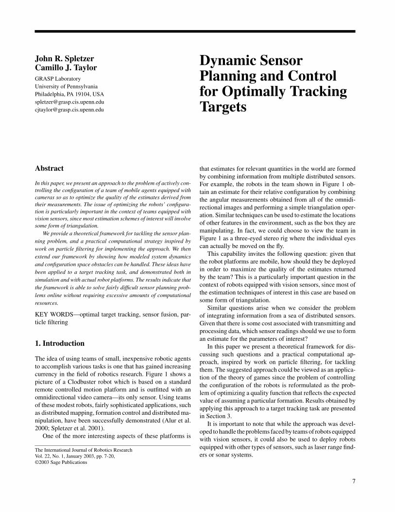
The idea of using teams of small, inexpensive robotic agentsto accomplish various tasks is one that has gained increasingcurrency in the field of robotics research. Figure 1 shows apicture of a Clodbuster robot which is based on a standardremote controlled motion platform and is outfitted with anomnidirectional video camera—its only sensor. Using teamsof these modest robots, fairly sophisticated applications, suchas distributed mapping, formation control and distributed ma-nipulation, have been successfully demonstrated (Alur et al.2000; Spletzer et al. 2001).

One of the more interesting aspects of these platforms is

The International Journal of Robotics ResearchVol. 22, No. 1, January 2003, pp. 7-20,©2003 Sage Publications

that estimates for relevant quantities in the world are formedby combining information from multiple distributed sensors.For example, the robots in the team shown in Figure 1 ob-tain an estimate for their relative configuration by combiningthe angular measurements obtained from all of the omnidi-rectional images and performing a simple triangulation oper-ation. Similar techniques can be used to estimate the locationsof other features in the environment, such as the box they aremanipulating. In fact, we could choose to view the team inFigure 1 as a three-eyed stereo rig where the individual eyescan actually be moved on the fly.

This capability invites the following question: given thatthe robot platforms are mobile, how should they be deployedin order to maximize the quality of the estimates returnedby the team? This is a particularly important question in thecontext of robots equipped with vision sensors, since most ofthe estimation techniques of interest in this case are based onsome form of triangulation.

Similar questions arise when we consider the problemof integrating information from a sea of distributed sensors.Given that there is some cost associated with transmitting andprocessing data, which sensor readings should we use to forman estimate for the parameters of interest?

In this paper we present a theoretical framework for dis-cussing such questions and a practical computational ap-proach, inspired by work on particle filtering, for tacklingthem. The suggested approach could be viewed as an applica-tion of the theory of games since the problem of controllingthe configuration of the robots is reformulated as the prob-lem of optimizing a quality function that reflects the expectedvalue of assuming a particular formation. Results obtained byapplying this approach to a target tracking task are presentedin Section 3.

It is important to note that while the approach was devel-oped to handle the problems faced by teams of robots equippedwith vision sensors, it could also be used to deploy robotsequipped with other types of sensors, such as laser range find-ers or sonar systems.

7

8 THE INTERNATIONAL JOURNAL OF ROBOTICS RESEARCH / January 2003

Fig. 1. A single Clodbuster robot (left) and the team performing a distributed manipulation task.

1.1. Related Work

The focus of this research is a probabilistic framework whichexploits the degrees of freedom afforded by robot mobilityto actively manage sensor positions for improved state esti-mation. We demonstrate its effectiveness in an optimal targettracking task. “Optimal tracking” can be defined using variousmetrics. We choose to minimize the expected error in trackingtarget positions. Since the measurements of multiple robotsare combined to estimate target pose, this relates strongly towork in sensor fusion.

In our target tracking task, robots rely on omnidirectionalcameras for tracking groups of targets. Merging measure-ments from multiple vision sensors for improved state estima-tion was considered by Bajcsy and others under the headingof Active Perception. Improvements were seen in various per-formance metrics, including ranging accuracy (Bajcsy 1988;Krotkov and Bajcsy 1993). Our framework can be viewed asan extension of this paradigm to distributed mobile robotics.

Durrant-Whyte and co-workers pioneered work in sensorfusion and robot localization. This yielded significant im-provements to methods used in mobile robot navigation, lo-calization and mapping (Majumder, Scheding, and Durrant-Whyte 2001; Dissanayake et al. 2001). Thrun and co-workershave also contributed significant research to these areas(Thrun 2001; Thrun et al. 2000). The work of both groups hasemphasized probabilistic techniques for data fusion—with arecent focus on particle filtering methods. Our approach isalso probabilistic, and it too leverages particle filtering meth-ods. However, our work distinguishes itself from traditionaldata fusion techniques in that the sensors themselves are ac-tively managed to improve the quality of the measurementsobtained prior to the data fusion phase, resulting in corre-sponding improvements in state estimation.

Since the sensors are actively managed, our work relatesto research in on-line sensor planning as well. Relevant to ourapproach was a methodology for distributed control proposed

by Parker (1999). This framework—Cooperative Multi-RobotObservation of Multiple Moving Targets (CMOMMT)—attempted to maximize the collective time that each targetwas being observed by at least one robot.

The theory of games has also provided inspiration for sim-ilar research in target tracking. The pursuit-evasion problemwas investigated by LaValle et al. (1997) and Fabiani et al.(2001). Both examined the task of maintaining target visibil-ity in a cluttered environment known a priori to the pursuer.LaValle’s approach generated trajectories that minimized aloss function which grew when the target became occluded.Fabiani’s motion strategy was based on the expected maxi-mum value of a corresponding utility function U . Of the two,Fabiani’s work is more relevant. The value of U was affectedby uncertainty in the target’s position, which was indirectlyaffected by uncertainty in the pursuer’s position. As a result,the pursuer trajectory was influenced not just by target posi-tion, but also by known landmark positions in the environmentwhich could be used to reduce uncertainty in target pose.

In all three of these cases, the optimization criterion wasbased on maintaining target observability, rather than the qual-ity of the observation. Additionally, the work of LaValle andFabiani was limited to the case of a single pursuer/evader. Intheory, both could be extended to multiple agents. However,in practice the resulting explosion in computational complex-ity would be prohibitive. In contrast, the complexity of ourframework is implementation-dependent, and may be tunedby the user to scale very efficiently in terms of the number ofrobots and targets.

In the next best view (NBV) problem, sensor placementis of primary concern (Pito 1999; Stamos and Allen 1998).Given, for example, previous range scans of an object, anNBV system attempts to determine the next best position ofthe scanner for acquiring the object’s complete surface geom-etry. As in our framework, the emphasis is optimizing sensorplacement. However, NBV is intended for use in a static en-vironment. Inherent in our approach is the ability to handle

Spletzer and Taylor / Dynamic Sensor Planning and Control 9

dynamic scenes which makes it more akin to a control law fordistributed sensors.

2. Developing the Framework

2.1. A Theoretical Approach

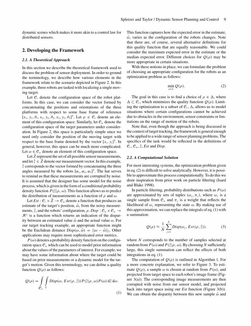
In this section we describe the theoretical framework used todiscuss the problem of sensor deployment. In order to groundthe terminology, we describe how various elements in theframework relate to the scenario depicted in Figure 2. In thisexample, three robots are tasked with localizing a single mov-ing target.

Let Cr denote the configuration space of the robot plat-forms. In this case, we can consider the vector formed byconcatenating the positions and orientations of the threeplatforms with respect to some base frame of reference[x1, y1, θ1, x2, y2, θ2, x3, y3, θ3]T. Let ρ ∈ Cr denote an ele-ment of this configuration space. Similarly, let Cw denote theconfiguration space of the target parameters under consider-ation. In Figure 2, this space is particularly simple since weneed only consider the position of the moving target withrespect to the base frame denoted by the vector [xt , yt ]T. Ingeneral, however, this space can be much more complicated.Let ω ∈ Cw denote an element of this configuration space.

Let Z represent the set of all possible sensor measurements,and let z ∈ Z denote our measurement vector. In this example,z corresponds to the vector formed by concatenating the threeangles measured by the robots [α1, α2, α3]T. The hat servesto remind us that these measurements are corrupted by noise.It is assumed that the designer has some model for the noiseprocess, which is given in the form of a conditional probabilitydensity function P(z|ρ, ω). This function allows us to predictthe distribution of measurements as a function of ρ and ω.

Let Est : Cr × Z → Cw denote a function that produces anestimate of the target’s position, ω, from the noisy measure-ments, z, and the robots’ configuration, ρ. Disp : Cw ×Cw →R+ is a function which returns an indication of the dispar-ity between an estimated value ω and the actual value ω. Forour target tracking example, an appropriate function mightbe the Euclidean distance Disp(ω, ω) = ||ω − ω||2. Otherapplications may require more sophisticated error metrics.P(ω)denotes a probability density function on the configu-

ration space Cw which can be used to model prior informationabout the values of the parameters of interest. For example, wemay have some information about where the target could bebased on prior measurements or a dynamic model for the tar-get’s motion. Given this terminology, we can define a qualityfunction Q(ρ) as follows:

Q(ρ) =∫

Cw

∫

Z

Disp(ω,Est (ρ, z))P (z|ρ, ω)P (ω) dz dω.

(1)

This function captures how the expected error in the estimate,ω, varies as the configuration of the robots changes. Notethat there are, of course, several alternative definitions forthis quality function that are equally reasonable. We couldconsider the maximum expected error in the estimate or themedian expected error. Different choices for Q(ρ) may bemore appropriate in certain situations.

With these notions in place, we can formulate the problemof choosing an appropriate configuration for the robots as anoptimization problem as follows:

minρ∈�

Q(ρ). (2)

The goal in this case is to find a choice of ρ ∈ �, where� ⊂ Cr , which minimizes the quality function Q(ρ). Limit-ing the optimization to a subset of Cr , �, allows us to modelsituations where certain configurations cannot be achieveddue to obstacles in the environment, sensor constraints or lim-itations on the range of motion of the robots.

Note that, even though the approach is being discussed inthe context of target tracking, the framework is general enoughto be applied to a wide range of sensor planning problems. Thespecifics of the task would be reflected in the definitions ofCr , Cw, z, Est and Disp.

2.2. A Computational Solution

For most interesting systems, the optimization problem givenin eq. (2) is difficult to solve analytically. However, it is possi-ble to approximate this process computationally. To do this wedraw inspiration from prior work on particle filtering (Isardand Blake 1998).

In particle filtering, probability distributions such as P(ω)are approximated by sets of tuples (ωj , πj ), where ωj is asingle sample from Cw and πj is a weight that reflects thelikelihood of ωj representing the state ω. By making use ofthis approximation, we can replace the integrals of eq. (1) witha summation:

Q(ρ) ≈ 1

N

N∑j=1

Disp(ωj , Est (ρ, z)). (3)

where N corresponds to the number of samples selected atrandom fromP(ω) andP(z|ρ, ω). By choosingN sufficientlylarge, this single summation can reflect the effects of bothintegrations in eq. (1).

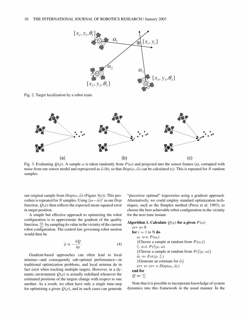
The computation of Q(ρ) is outlined in Algorithm 1. Fora more concrete explanation, we refer to Figure 3. To esti-mate Q(ρ), a sample ω is chosen at random from P(ω), andprojected from target space to each robot’s image frame (Fig-ure 3(a)). The corresponding image measurements are thencorrupted with noise from our sensor model, and projectedback into target space using our Est function (Figure 3(b)).We can obtain the disparity between this new sample ω and

10 THE INTERNATIONAL JOURNAL OF ROBOTICS RESEARCH / January 2003

T ],[ tt yx

],,[ 333 θyx],,[ 222 θyx

],,[ 111 θyx1α

2α3α

12

3

Fig. 2. Target localization by a robot team.

(a) (b) (c)Fig. 3. Evaluating Q(ρ). A sample ω is taken randomly from P(ω) and projected into the sensor frames (a), corrupted withnoise from our sensor model and reprojected as ω (b), so that Disp(ω, ω) can be calculated (c). This is repeated for N randomsamples.

our original sample from Disp(ω, ω) (Figure 3(c)). This pro-cedure is repeated forN samples. Using ||ω−ω||2 as our Dispfunction, Q(ρ) then reflects the expected mean-squared errorin target position.

A simple but effective approach to optimizing the robotconfiguration is to approximate the gradient of the qualityfunction, ∂Q

∂ρ, by sampling its value in the vicinity of the current

robot configuration. The control law governing robot motionwould then be

ρ ∝ −∂Q

∂ρ. (4)

Gradient-based approaches can often lead to localminima—and consequently sub-optimal performance—intraditional optimization problems, and local minima do infact exist when tracking multiple targets. However, in a dy-namic environment Q(ρ) is actually redefined whenever theestimated positions of the targets change with respect to oneanother. As a result, we often have only a single time-stepfor optimizing a given Q(ρ), and in such cases can generate

“piecewise optimal” trajectories using a gradient approach.Alternatively, we could employ standard optimization tech-niques, such as the Simplex method (Press et al. 1993), tochoose the best achievable robot configuration in the vicinityfor the next time instant.

Algorithm 1. Calculate Q(ρ) for a given P(ω)err ⇐ 0for i = 1 to N doωi ⇐∈ P(ωi)

{Choose a sample at random from P(ωi)}zi ⇐∈ P(z|ρ, ω){Choose a sample at random from P(z|ρ, ω)}ωi ⇐ Est(ρ, zi)

{Generate an estimate for ω}err ⇐ err + Disp(ωi, ωi)

end forQ ⇐ err

N

Note that it is possible to incorporate knowledge of systemdynamics into this framework in the usual manner. In the

Spletzer and Taylor / Dynamic Sensor Planning and Control 11

CONDENSATION algorithm described by Isard and Blake(1998), a particle distributionP(ω) is propagated at each time-step according to a known dynamic model. This same P(ω)serves as the assumed input for our framework, and establishesa complementary relationship between sensing and control,as the same particle sets used for tracking targets are alsoused to control the robot team for improving future trackingestimates.

3. Experimental Results

3.1. Simulation Experiments

In order to demonstrate the utility of the proposed framework,we first apply it to three sensor planning problems in simu-lation: tracking a single point target; tracking multiple pointtargets; and tracking a box. We then extend the point targettracking problem by incorporating a dynamical model for thetarget. Finally, we integrate motion planning techniques forlocal obstacle avoidance and we demonstrate target trackingin a cluttered workspace. Each of these scenarios is explainedin more detail below.

We have assumed in all of these scenarios that the robotscan accurately measure their positions and orientations withrespect to one another, since it is the robot positions relativeto the targets that are of interest. Note that we could considerthe error in the positioning of the robots within this frame-work by adding extra noise terms to the measurements or byincluding the configuration of the robots as part of the stateto be estimated.

3.1.1. Tracking a Single Point Target

For the first scenario, we consider two robots equipped withomnidirectional cameras, and tasked with tracking a singletarget. Cr represents the concatenation of the robot positions,Cw the target position, and z the two angles to the target mea-sured by the members of the robot team. We assume z tobe corrupted with random noise generated from our sensormodel. Est(ρ, z) returns an estimate for the target position,ω, which minimizes the squared disparity with the measure-ments, z, and Disp(ω, ω) simply returns the Euclidean dis-tance between the estimated target position and the actualvalue.

In our simulations, robot motions are constrained by themaximum robot velocity and the robot positions are limited bymandating a minimum standoff distance to the target. Theseserve to define the valid configuration space for the robots,�.Below, we provide results from Matlab simulations for tworobots with both static and dynamic targets. For these trials,100 exemplars were used to approximateP(ω), and the sensormodel (for all trials) was assumed to be Gaussian noise withσ = 1◦.

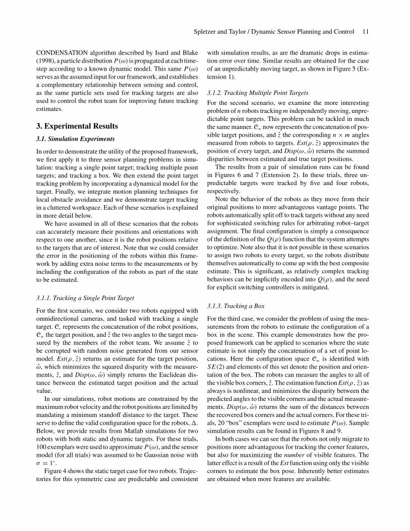
Figure 4 shows the static target case for two robots. Trajec-tories for this symmetric case are predictable and consistent

with simulation results, as are the dramatic drops in estima-tion error over time. Similar results are obtained for the caseof an unpredictably moving target, as shown in Figure 5 (Ex-tension 1).

3.1.2. Tracking Multiple Point Targets

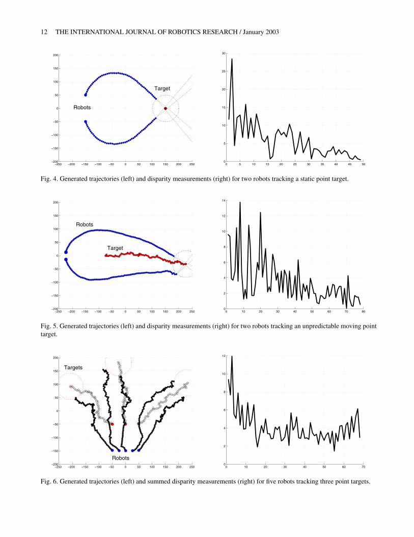
For the second scenario, we examine the more interestingproblem of n robots trackingm independently moving, unpre-dictable point targets. This problem can be tackled in muchthe same manner. Cw now represents the concatenation of pos-sible target positions, and z the corresponding n × m anglesmeasured from robots to targets. Est(ρ, z) approximates theposition of every target, and Disp(ω, ω) returns the summeddisparities between estimated and true target positions.

The results from a pair of simulation runs can be foundin Figures 6 and 7 (Extension 2). In these trials, three un-predictable targets were tracked by five and four robots,respectively.

Note the behavior of the robots as they move from theiroriginal positions to more advantageous vantage points. Therobots automatically split off to track targets without any needfor sophisticated switching rules for arbitrating robot–targetassignment. The final configuration is simply a consequenceof the definition of theQ(ρ) function that the system attemptsto optimize. Note also that it is not possible in these scenariosto assign two robots to every target, so the robots distributethemselves automatically to come up with the best compositeestimate. This is significant, as relatively complex trackingbehaviors can be implicitly encoded into Q(ρ), and the needfor explicit switching controllers is mitigated.

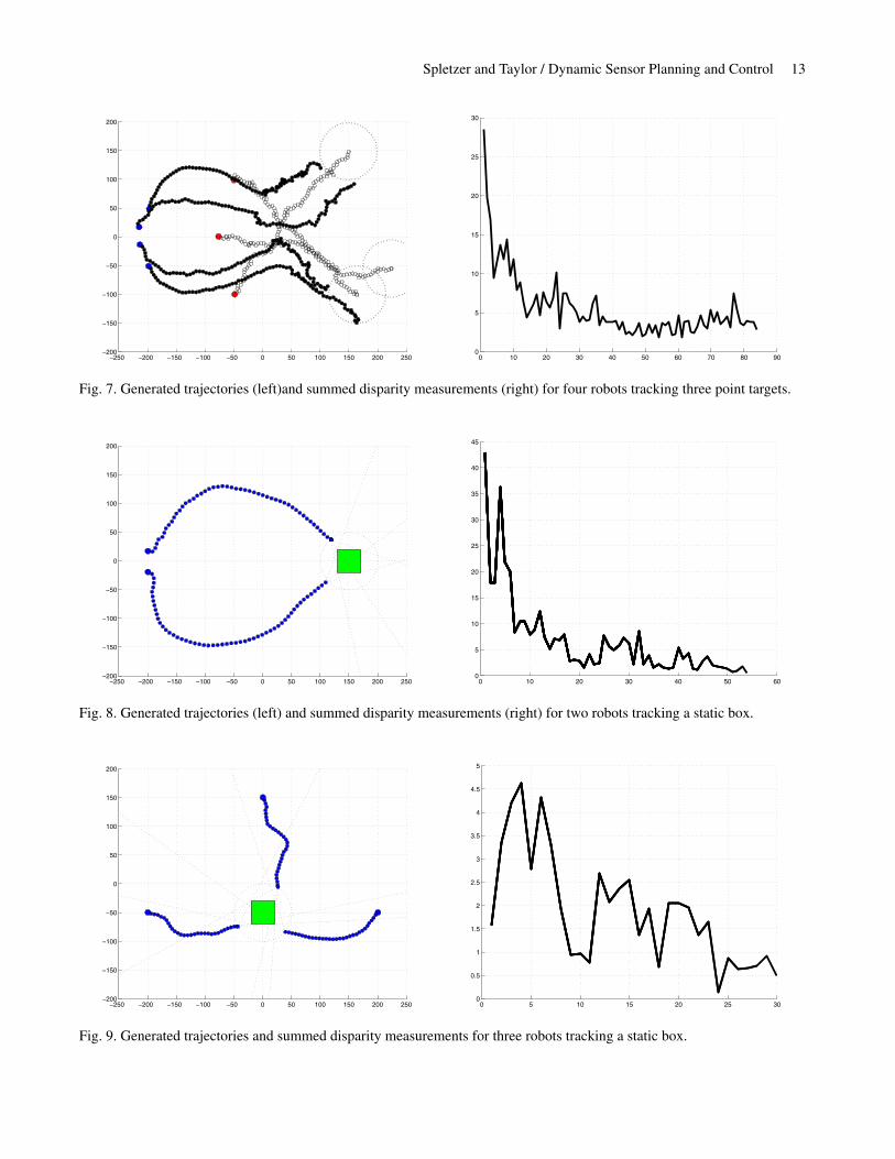
3.1.3. Tracking a Box

For the third case, we consider the problem of using the mea-surements from the robots to estimate the configuration of abox in the scene. This example demonstrates how the pro-posed framework can be applied to scenarios where the stateestimate is not simply the concatenation of a set of point lo-cations. Here the configuration space Cw is identified withSE(2) and elements of this set denote the position and orien-tation of the box. The robots can measure the angles to all ofthe visible box corners, z. The estimation function Est(ρ, z) asalways is nonlinear, and minimizes the disparity between thepredicted angles to the visible corners and the actual measure-ments. Disp(ω, ω) returns the sum of the distances betweenthe recovered box corners and the actual corners. For these tri-als, 20 “box” exemplars were used to estimate P(ω). Samplesimulation results can be found in Figures 8 and 9.

In both cases we can see that the robots not only migrate topositions more advantageous for tracking the corner features,but also for maximizing the number of visible features. Thelatter effect is a result of the Est function using only the visiblecorners to estimate the box pose. Inherently better estimatesare obtained when more features are available.

12 THE INTERNATIONAL JOURNAL OF ROBOTICS RESEARCH / January 2003

−250 −200 −150 −100 −50 0 50 100 150 200 250−200

−150

−100

−50

0

50

100

150

200

Robots

Target

0 5 10 15 20 25 30 35 40 45 500

5

10

15

20

25

30

Fig. 4. Generated trajectories (left) and disparity measurements (right) for two robots tracking a static point target.

−250 −200 −150 −100 −50 0 50 100 150 200 250−200

−150

−100

−50

0

50

100

150

200

Robots

Target

0 10 20 30 40 50 60 70 800

2

4

6

8

10

12

14

Fig. 5. Generated trajectories (left) and disparity measurements (right) for two robots tracking an unpredictable moving pointtarget.

−250 −200 −150 −100 −50 0 50 100 150 200 250−200

−150

−100

−50

0

50

100

150

200

Robots

Targets

0 10 20 30 40 50 60 700

2

4

6

8

10

12

Fig. 6. Generated trajectories (left) and summed disparity measurements (right) for five robots tracking three point targets.

Spletzer and Taylor / Dynamic Sensor Planning and Control 13

−250 −200 −150 −100 −50 0 50 100 150 200 250−200

−150

−100

−50

0

50

100

150

200

0 10 20 30 40 50 60 70 80 900

5

10

15

20

25

30

Fig. 7. Generated trajectories (left)and summed disparity measurements (right) for four robots tracking three point targets.

−250 −200 −150 −100 −50 0 50 100 150 200 250−200

−150

−100

−50

0

50

100

150

200

0 10 20 30 40 50 600

5

10

15

20

25

30

35

40

45

Fig. 8. Generated trajectories (left) and summed disparity measurements (right) for two robots tracking a static box.

−250 −200 −150 −100 −50 0 50 100 150 200 250−200

−150

−100

−50

0

50

100

150

200

0 5 10 15 20 25 300

0.5

1

1.5

2

2.5

3

3.5

4

4.5

5

Fig. 9. Generated trajectories and summed disparity measurements for three robots tracking a static box.

14 THE INTERNATIONAL JOURNAL OF ROBOTICS RESEARCH / January 2003

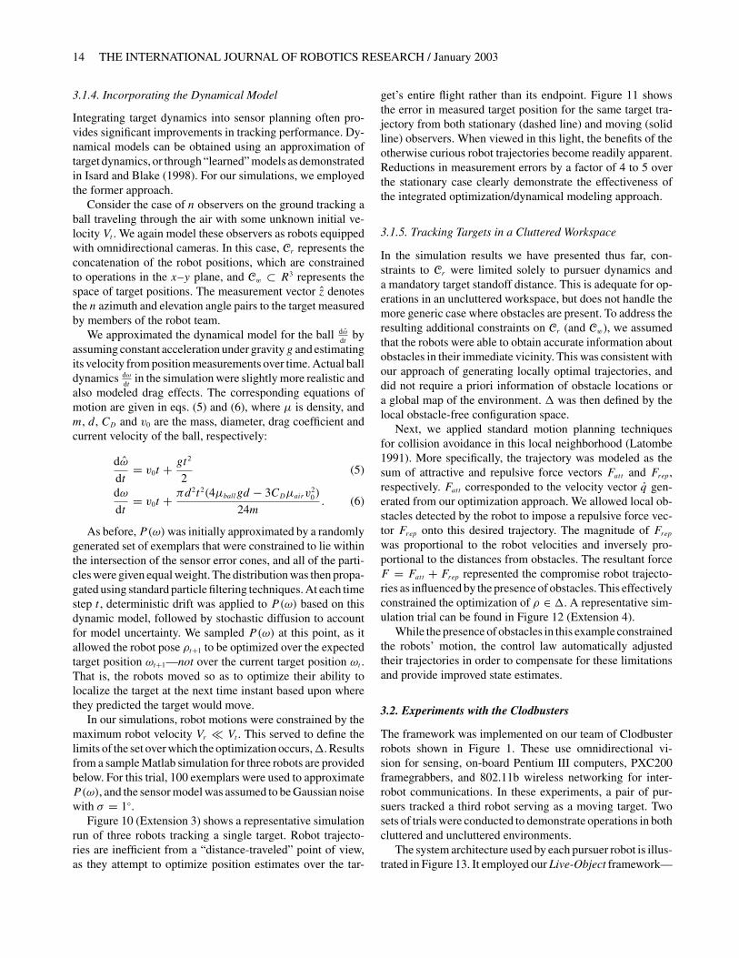
3.1.4. Incorporating the Dynamical Model

Integrating target dynamics into sensor planning often pro-vides significant improvements in tracking performance. Dy-namical models can be obtained using an approximation oftarget dynamics, or through “learned” models as demonstratedin Isard and Blake (1998). For our simulations, we employedthe former approach.

Consider the case of n observers on the ground tracking aball traveling through the air with some unknown initial ve-locity Vt . We again model these observers as robots equippedwith omnidirectional cameras. In this case, Cr represents theconcatenation of the robot positions, which are constrainedto operations in the x–y plane, and Cw ⊂ R3 represents thespace of target positions. The measurement vector z denotesthe n azimuth and elevation angle pairs to the target measuredby members of the robot team.

We approximated the dynamical model for the ball dωdt

byassuming constant acceleration under gravityg and estimatingits velocity from position measurements over time. Actual balldynamics dω

dtin the simulation were slightly more realistic and

also modeled drag effects. The corresponding equations ofmotion are given in eqs. (5) and (6), where µ is density, andm, d, CD and v0 are the mass, diameter, drag coefficient andcurrent velocity of the ball, respectively:

dω

dt= v0t + gt 2

2(5)

dω

dt= v0t + πd2t2(4µballgd − 3CDµairv

20)

24m. (6)

As before,P(ω)was initially approximated by a randomlygenerated set of exemplars that were constrained to lie withinthe intersection of the sensor error cones, and all of the parti-cles were given equal weight. The distribution was then propa-gated using standard particle filtering techniques. At each timestep t , deterministic drift was applied to P(ω) based on thisdynamic model, followed by stochastic diffusion to accountfor model uncertainty. We sampled P(ω) at this point, as itallowed the robot pose ρt+1 to be optimized over the expectedtarget position ωt+1—not over the current target position ωt .That is, the robots moved so as to optimize their ability tolocalize the target at the next time instant based upon wherethey predicted the target would move.

In our simulations, robot motions were constrained by themaximum robot velocity Vr � Vt . This served to define thelimits of the set over which the optimization occurs,�. Resultsfrom a sample Matlab simulation for three robots are providedbelow. For this trial, 100 exemplars were used to approximateP(ω), and the sensor model was assumed to be Gaussian noisewith σ = 1◦.

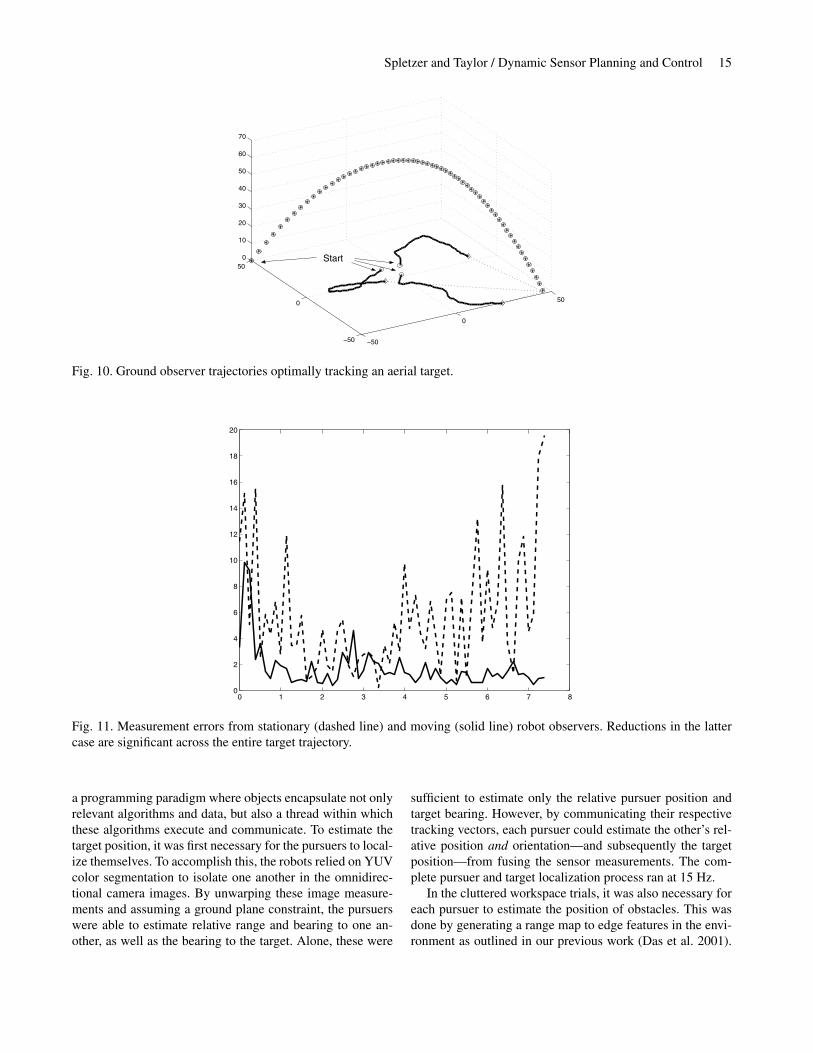
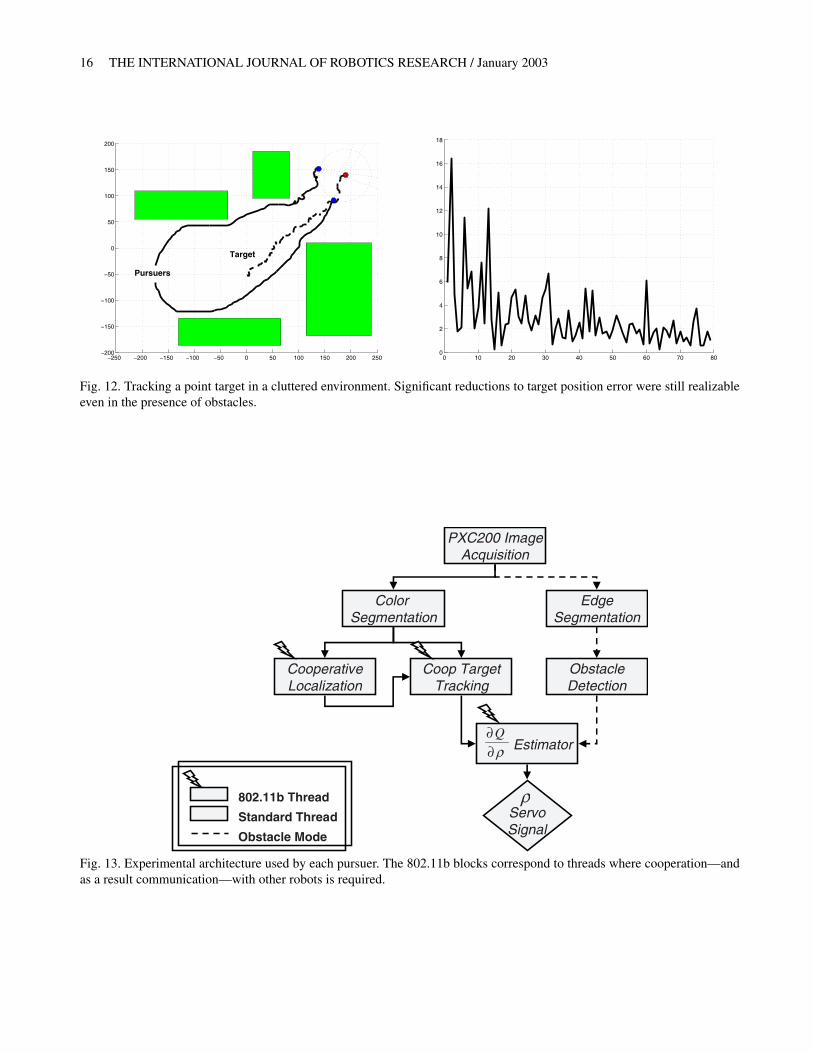
Figure 10 (Extension 3) shows a representative simulationrun of three robots tracking a single target. Robot trajecto-ries are inefficient from a “distance-traveled” point of view,as they attempt to optimize position estimates over the tar-

get’s entire flight rather than its endpoint. Figure 11 showsthe error in measured target position for the same target tra-jectory from both stationary (dashed line) and moving (solidline) observers. When viewed in this light, the benefits of theotherwise curious robot trajectories become readily apparent.Reductions in measurement errors by a factor of 4 to 5 overthe stationary case clearly demonstrate the effectiveness ofthe integrated optimization/dynamical modeling approach.

3.1.5. Tracking Targets in a Cluttered Workspace

In the simulation results we have presented thus far, con-straints to Cr were limited solely to pursuer dynamics anda mandatory target standoff distance. This is adequate for op-erations in an uncluttered workspace, but does not handle themore generic case where obstacles are present. To address theresulting additional constraints on Cr (and Cw), we assumedthat the robots were able to obtain accurate information aboutobstacles in their immediate vicinity. This was consistent withour approach of generating locally optimal trajectories, anddid not require a priori information of obstacle locations ora global map of the environment. � was then defined by thelocal obstacle-free configuration space.

Next, we applied standard motion planning techniquesfor collision avoidance in this local neighborhood (Latombe1991). More specifically, the trajectory was modeled as thesum of attractive and repulsive force vectors Fatt and Frep,respectively. Fatt corresponded to the velocity vector q gen-erated from our optimization approach. We allowed local ob-stacles detected by the robot to impose a repulsive force vec-tor Frep onto this desired trajectory. The magnitude of Frep

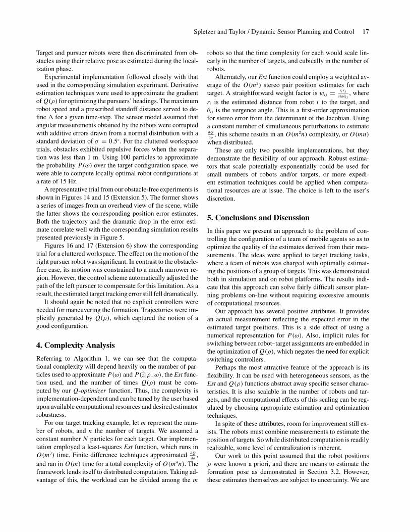
was proportional to the robot velocities and inversely pro-portional to the distances from obstacles. The resultant forceF = Fatt + Frep represented the compromise robot trajecto-ries as influenced by the presence of obstacles. This effectivelyconstrained the optimization of ρ ∈ �. A representative sim-ulation trial can be found in Figure 12 (Extension 4).

While the presence of obstacles in this example constrainedthe robots’ motion, the control law automatically adjustedtheir trajectories in order to compensate for these limitationsand provide improved state estimates.

3.2. Experiments with the Clodbusters

The framework was implemented on our team of Clodbusterrobots shown in Figure 1. These use omnidirectional vi-sion for sensing, on-board Pentium III computers, PXC200framegrabbers, and 802.11b wireless networking for inter-robot communications. In these experiments, a pair of pur-suers tracked a third robot serving as a moving target. Twosets of trials were conducted to demonstrate operations in bothcluttered and uncluttered environments.

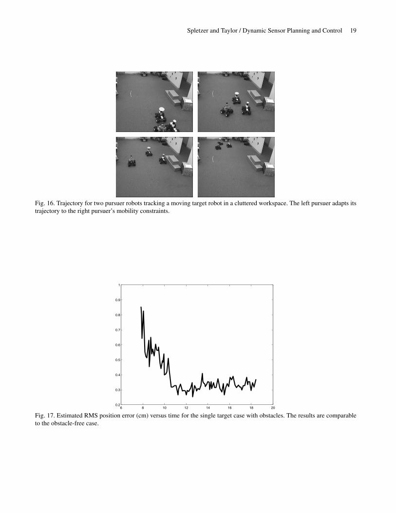
The system architecture used by each pursuer robot is illus-trated in Figure 13. It employed our Live-Object framework—

Spletzer and Taylor / Dynamic Sensor Planning and Control 15

−50

0

50

−50

0

500

10

20

30

40

50

60

70

Start

Fig. 10. Ground observer trajectories optimally tracking an aerial target.

0 1 2 3 4 5 6 7 80

2

4

6

8

10

12

14

16

18

20

Fig. 11. Measurement errors from stationary (dashed line) and moving (solid line) robot observers. Reductions in the lattercase are significant across the entire target trajectory.

a programming paradigm where objects encapsulate not onlyrelevant algorithms and data, but also a thread within whichthese algorithms execute and communicate. To estimate thetarget position, it was first necessary for the pursuers to local-ize themselves. To accomplish this, the robots relied on YUVcolor segmentation to isolate one another in the omnidirec-tional camera images. By unwarping these image measure-ments and assuming a ground plane constraint, the pursuerswere able to estimate relative range and bearing to one an-other, as well as the bearing to the target. Alone, these were

sufficient to estimate only the relative pursuer position andtarget bearing. However, by communicating their respectivetracking vectors, each pursuer could estimate the other’s rel-ative position and orientation—and subsequently the targetposition—from fusing the sensor measurements. The com-plete pursuer and target localization process ran at 15 Hz.

In the cluttered workspace trials, it was also necessary foreach pursuer to estimate the position of obstacles. This wasdone by generating a range map to edge features in the envi-ronment as outlined in our previous work (Das et al. 2001).

16 THE INTERNATIONAL JOURNAL OF ROBOTICS RESEARCH / January 2003

−250 −200 −150 −100 −50 0 50 100 150 200 250−200

−150

−100

−50

0

50

100

150

200

Target

Pursuers

0 10 20 30 40 50 60 70 800

2

4

6

8

10

12

14

16

18

Fig. 12. Tracking a point target in a cluttered environment. Significant reductions to target position error were still realizableeven in the presence of obstacles.

PXC200 ImageAcquisition

Color Segmentation

EdgeSegmentation

CooperativeLocalization

ObstacleDetection

Coop TargetTracking

Standard Thread

802.11b Thread

Obstacle Mode

ρ∂∂Q

Estimator

ρ ServoSignal

Fig. 13. Experimental architecture used by each pursuer. The 802.11b blocks correspond to threads where cooperation—andas a result communication—with other robots is required.

Spletzer and Taylor / Dynamic Sensor Planning and Control 17

Target and pursuer robots were then discriminated from ob-stacles using their relative pose as estimated during the local-ization phase.

Experimental implementation followed closely with thatused in the corresponding simulation experiment. Derivativeestimation techniques were used to approximate the gradientofQ(ρ) for optimizing the pursuers’ headings. The maximumrobot speed and a prescribed standoff distance served to de-fine � for a given time-step. The sensor model assumed thatangular measurements obtained by the robots were corruptedwith additive errors drawn from a normal distribution with astandard deviation of σ = 0.5◦. For the cluttered workspacetrials, obstacles exhibited repulsive forces when the separa-tion was less than 1 m. Using 100 particles to approximatethe probability P(ω) over the target configuration space, wewere able to compute locally optimal robot configurations ata rate of 15 Hz.

A representative trial from our obstacle-free experiments isshown in Figures 14 and 15 (Extension 5). The former showsa series of images from an overhead view of the scene, whilethe latter shows the corresponding position error estimates.Both the trajectory and the dramatic drop in the error esti-mate correlate well with the corresponding simulation resultspresented previously in Figure 5.

Figures 16 and 17 (Extension 6) show the correspondingtrial for a cluttered workspace. The effect on the motion of theright pursuer robot was significant. In contrast to the obstacle-free case, its motion was constrained to a much narrower re-gion. However, the control scheme automatically adjusted thepath of the left pursuer to compensate for this limitation. As aresult, the estimated target tracking error still fell dramatically.

It should again be noted that no explicit controllers wereneeded for maneuvering the formation. Trajectories were im-plicitly generated by Q(ρ), which captured the notion of agood configuration.

4. Complexity Analysis

Referring to Algorithm 1, we can see that the computa-tional complexity will depend heavily on the number of par-ticles used to approximate P(ω) and P(z|ρ, ω), the Est func-tion used, and the number of times Q(ρ) must be com-puted by our Q-optimizer function. Thus, the complexity isimplementation-dependent and can be tuned by the user basedupon available computational resources and desired estimatorrobustness.

For our target tracking example, let m represent the num-ber of robots, and n the number of targets. We assumed aconstant number N particles for each target. Our implemen-tation employed a least-squares Est function, which runs inO(m3) time. Finite difference techniques approximated ∂Q

∂ρ,

and ran in O(m) time for a total complexity of O(m4n). Theframework lends itself to distributed computation. Taking ad-vantage of this, the workload can be divided among the m

robots so that the time complexity for each would scale lin-early in the number of targets, and cubically in the number ofrobots.

Alternately, our Est function could employ a weighted av-erage of the O(m2) stereo pair position estimates for eachtarget. A straightforward weight factor is wij = ri rj

sinθij, where

ri is the estimated distance from robot i to the target, andθij is the vergence angle. This is a first-order approximationfor stereo error from the determinant of the Jacobian. Usinga constant number of simultaneous perturbations to estimate∂Q

∂ρ, this scheme results in an O(m2n) complexity, or O(mn)

when distributed.These are only two possible implementations, but they

demonstrate the flexibility of our approach. Robust estima-tors that scale potentially exponentially could be used forsmall numbers of robots and/or targets, or more expedi-ent estimation techniques could be applied when computa-tional resources are at issue. The choice is left to the user’sdiscretion.

5. Conclusions and Discussion

In this paper we present an approach to the problem of con-trolling the configuration of a team of mobile agents so as tooptimize the quality of the estimates derived from their mea-surements. The ideas were applied to target tracking tasks,where a team of robots was charged with optimally estimat-ing the positions of a group of targets. This was demonstratedboth in simulation and on robot platforms. The results indi-cate that this approach can solve fairly difficult sensor plan-ning problems on-line without requiring excessive amountsof computational resources.

Our approach has several positive attributes. It providesan actual measurement reflecting the expected error in theestimated target positions. This is a side effect of using anumerical representation for P(ω). Also, implicit rules forswitching between robot–target assignments are embedded inthe optimization of Q(ρ), which negates the need for explicitswitching controllers.

Perhaps the most attractive feature of the approach is itsflexibility. It can be used with heterogeneous sensors, as theEst and Q(ρ) functions abstract away specific sensor charac-teristics. It is also scalable in the number of robots and tar-gets, and the computational effects of this scaling can be reg-ulated by choosing appropriate estimation and optimizationtechniques.

In spite of these attributes, room for improvement still ex-ists. The robots must combine measurements to estimate theposition of targets. So while distributed computation is readilyrealizable, some level of centralization is inherent.

Our work to this point assumed that the robot positionsρ were known a priori, and there are means to estimate theformation pose as demonstrated in Section 3.2. However,these estimates themselves are subject to uncertainty. We are

18 THE INTERNATIONAL JOURNAL OF ROBOTICS RESEARCH / January 2003

Fig. 14. Trajectory for two pursuer robots tracking a moving target robot in an obstacle-free environment.

12 14 16 18 20 22 24 26 280.2

0.3

0.4

0.5

0.6

0.7

0.8

0.9

1

Fig. 15. Estimated RMS position error (cm) versus time for the single target case.

Spletzer and Taylor / Dynamic Sensor Planning and Control 19

Fig. 16. Trajectory for two pursuer robots tracking a moving target robot in a cluttered workspace. The left pursuer adapts itstrajectory to the right pursuer’s mobility constraints.

6 8 10 12 14 16 18 200.2

0.3

0.4

0.5

0.6

0.7

0.8

0.9

1

Fig. 17. Estimated RMS position error (cm) versus time for the single target case with obstacles. The results are comparableto the obstacle-free case.

20 THE INTERNATIONAL JOURNAL OF ROBOTICS RESEARCH / January 2003

currently reposing the problem within our framework as a si-multaneous localization and target tracking task to addressthis.

The approach was applied to target tracking tasks in bothopen and cluttered workspaces. However, the latter was ac-complished by merging with traditional motion planning tech-niques. As a result, it was subject to similar shortcomings (e.g.,becoming trapped in local minima). Additionally, our work incluttered environments only addressed issues relating to mo-tion planning and not occluding obstacles. The latter topic isthe subject of ongoing research.

Lastly, to this point we have assumed a sensor model withan omnidirectional field of view (FOV). Adapting our ap-proach to limited FOV sensors involves assimilating optimalassignment techniques with trajectory generation. This is alsothe topic of ongoing work.

Appendix: Index to Multimedia Extensions

The multimedia extension page is found at http://www.ijrr.org.

Table of Multimedia ExtensionsExtension Type Description

1 Video Simulation of two robots op-timally tracking an unpre-dictable point target

2 Video Simulation of four robots op-timally tracking three unpre-dictable point targets

3 Video Simulation of three groundobservers using a dynamicalmodel to optimally track anaerial target

4 Video Simulation of tracking a pointtarget in a cluttered workspace

5 Video Experimental trial with twopursuer robots tracking a thirdtarget robot in an obstacle-freeworkspace

6 Video Experimental trial with twopursuer robots tracking a thirdtarget robot in a clutteredworkspace

Acknowledgments

This material is based upon work supported by the Na-tional Science Foundation under a CAREER Grant (GrantNo 9875867) and by DARPA under the MARS program.

ReferencesAlur, R. et al. December 2000. A framework and architec-

ture for multi-robot coordination. In Proceedings of the

7th International Symposium on Experimental Robotics,Honolulu, Hawaii.

Bajcsy, R. August 1988. Active perception. In Proceedingsof the IEEE, Special Issue on Computer Vision 76(8):996–1005.

Das, A. et al. May 2001. Real-time vision based control ofa non-holonomic robot. In Proceedings of the IEEE Inter-national Conference on Robotics and Automation, Seoul,Korea. pp. 1714–1719.

Dissanayake, G., Newman, P., Durrant-Whyte, H., andCsorba, M. 2001. A solution to the simultaneous local-ization and map building. IEEE Transactions on Roboticsand Automation 17(3):229–241.

Fabiani, P., Gonzalez-Banos, H., Latombe, J., and Lin, D.2001. Tracking a partially predictable object with uncer-tainties and visibility constraints. Journal of AutonomousRobots 38(1):31–48.

Isard, M., and Blake, A. 1998. Condensation–conditional den-sity propagation for visual tracking. International Journalof Computer Vision 29(1):5–28.

Krotkov, E., and Bajcsy, R. 1993. Active vision for reliableranging: Cooperating focus, stereo, and vergence. Interna-tional Journal of Computer Vision 11(2):187–203.

Latombe, J. 1991. Robot Motion Planning. Kluwer Academic,Dordrecht.

LaValle, S., Gonzalez-Banos, H., Becker, C., and Latombe,J. April 1997. Motion strategies for maintaining visibil-ity of a moving target. In Proceeding of the IEEE Inter-national Conference on Robotics and Automation, Albu-querque, NM. pp. 731–736.

Majumder, S., Scheding, S., and Durrant-Whyte, H. 2001.Multi-sensor data fusion for underwater navigation.Robotics and Autonomous Systems 35(1):97–108.

Parker, L. 1999. Cooperative robotics for multi-target obser-vation. Intelligent Automation and Soft Computing 5(1):5–19.

Pito, R. 1999. A solution to the next best view problem for au-tomated surface acquisition. IEEE Transactions on PatternAnalysis and Machine Intelligence 21(10):1016–1030.

Press, W., Teukolsky, S., Vetterling, W., and Flannery, B.1993. Numerical Recipes in C. Cambridge UniversityPress, Cambridge.

Spletzer, J. et al. October 2001. Cooperative localizationand control for multi-robot manipulation. In InternationalConference on Intelligent Robots and Systems, Maui,Hawaii.

Stamos, I., and Allen, P. June 1998. Interactive sensor plan-ning. In Computer Vision and Pattern Recognition Confer-ence, Santa Barbara, CA. pp. 489–495.

Thrun, S. 2001. A probabilistic online mapping algorithm forteams of mobile robots. International Journal of RoboticsResearch 20(5):335–363.

Thrun, S., Fox, D., Burgard, W., and Dellaert, F. 2000. Ro-bust Monte Carlo localization for mobile robots. ArtificialIntelligence 128(1–2):99–141.