Divide and Conquer Spot Noise

Wim de LeeuwRobert van Liere

Center for Mathematics and Computer Science CWI,P.O. Box 94097, 1090 GB Amsterdam, Netherlands

Abstract

The design and implementation of an interactive spot noise algorithm ispresented. Spot noise is a technique which utilizes texture for the visual-ization of flow fields. Various design tradeoffs are discussed that allow anoptimal implementation on a range of high end graphical workstations.

Two applications are given: the steering of a smog prediction simulationand browsing a very large data set resulting from a direct numerical simula-tion of turbulence. These applications provide the motivation for the need ofinteractive visualization techniques.Keywords: interactive scientific visualization, flow visualization, high per-formance computing, atmospheric simulation, direct numerical simulation.

1 Introduction.

During the last decade the need for flow visualization techniques for representingvector fields has grown substantially. The reason for this isthat increasingly com-plex phenomena are simulated and that the resulting data sets are becoming moredifficult to interpret. The visualization community has developed many accurateand robust flow visualization methods to display these data sets [1]. Simultane-ously, there is also a growing demand for interactive computing in which users cancontrol various aspects of the application [2]. The role of computational steeringand browsing of very large scientific data bases are two examples of this demand.Both examples require highly interactive visualization toaccommodate the require-ments for adequate animation and feedback rates.

Spot noise is a texture synthesis technique which can be usedto visualize flowfields [3]. Rather than mapping the underlying vector field toproduce colored ge-ometric objects, spot noise uses texture. The primary advantage over other flow

1

visualization techniques is that texture can give a continuous view of a 2D field op-posed to visualization at only discrete positions, as with arrow plots or streamlines.The basic idea is that if many particles are used to representthe flow, the individualparticles can no longer be discerned and texture is perceived instead. Spot noisegenerates texture by adding a large number of randomly positioned spots with arandom intensity. A spot is defined to be any geometric shape,but usually a smallcircle is used. Properties of the spot directly control the properties of the texture.Therefore, by modifying the shape of the spot as a function ofthe data, the data arevisualized by texture.

The downside of spot noise is that it is very computationallyexpensive. A largenumber of particle paths and particle positions must be calculated, spots must betransformed, scan converted, textured and blended. Previously, spot noise textureswere generated as a preprocessing step and the resulting sequence of images wereanimated. In this paper we discuss the implementation of an interactive spot noisealgorithm. Textures are generated on the fly so that spot noise can be used ininteractive applications.

Many graphical operations are needed during texture synthesis. Graphics sub-systems are designed to handle these operations efficiently. On the other hand, par-ticle position calculations are best computed on general purpose processors. Thisresults in many design software vs. hardware tradeoffs. We discuss these tradeoffs.

The paper is organized as follows: first, the underlying ideas of spot noise arereviewed. We then present and discuss the divide and conquerspot noise algorithmand its implementation. Finally, we apply the algorithm to two applications: thesteering of a smog prediction simulation and browsing a verylarge data set result-ing from a direct numerical simulation of turbulence. Theseapplications provideour motivation for an interactive implementation of the spot noise algorithm.

2 Spot noise overview.

We give a brief overview of the spot noise texture synthesis technique. A texturecan be characterized by a scalar functionf of positionx. A spot noise texture [3]is defined as f(x) =X aih(x� xi)in which h(x) is called the spot function. It is a function everywhere zeroexceptfor an area that is small compared to the texture size.ai is a random scaling factorwith a zero mean,xi is a random position. In non-mathematical terms: spots of

2

random intensity are drawn and blended together on random positions on a plane(figure 1).

Figure 1: Principle of spot noise: single spot (left) resulting texture (right)

The use of a spot as a basis texture synthesis has a number of convenient, usercontrollable, properties. First, the shape of a spot determines the characteristicsof the texture. By local variation of the spot shape, presentation of data becomespossible; in this way vector fields can be effectively visualized. Second, dynamicphenomena can be displayed via an animated sequence of spot noise images. Aspot noise animation of a flow field can be realized by associating a particle witheach spot position. A new frame in the animation sequence is determined by ad-vecting all particles over a small distance through the flow field.

Figure 2 is an example of how spot noise can be used to study theseparationof a wind field impinging on the front of a block (see section 5.2 for details).The question was to find regions where the flow passes over or under the block

Figure 2: Two views of the separation line of a wind field impinging on a block;default spot noise (top) using advected spot positions (bottom).

respectively. The top image shows the skin friction field on the block using the spotnoise algorithm with default parameters. By adjusting parameters related to spotposition and spot life cycle, the lower image is generated. Adjusting parameters

3

in this way provides the user with a mechanism to highlight certain aspects of theflow which may otherwise stay hidden.

In [4], enhancements to the original spot noise algorithm are given. Bent spotsallow spot noise to be used in highly irregular flows, such as in areas where cur-vature of the vector field is high. Instead of using a single textured polygon withfour vertices, bent spots use a textured mesh to represent the spot. The mesh isgenerated by tiling a surface generated by advecting a stream line in the flow. Thisis a computationally demanding technique because stream lines must be generatedand the mesh must be rendered for each spot. Other enhancements include spotfiltering and use of spot noise for non-uniform data grids.

Spot noise pipeline. Algorithmically, spot noise synthesis performs four steps(figure 3):

1. Read a data set of a vector field. For interactive scientificvisualization, thisstep may typically occur anywhere between 5 and 15 times a second.

2. Particle advection. The position of each particle is updated by advecting itby the flow field.

3. Texture synthesis. A spot is generated for each particle position. Each spotis transformed and assigned an intensity according to properties of the flowfield. All spots are scan converted and blended together to form a texturemap, after which additional spot filtering operations may beapplied to themap.

4. An image is rendered by mapping the texture onto a geometric surface. Othervisualization techniques may also be superimposed on the texture mappedobject.

render scene

generatetexture

a d v e c tpaticles

read data

0.8088 -0.041 0.003 4.7985 -10.634 16.7040.8088 -0.041 0.003 5.0153 -11.114 12.570

Figure 3: Spot noise pipeline; logical steps (top) and iconic representations (bot-tom).

4

Utilizing graphics hardware. The synthesis of spot noise texture can be con-sidered as rendering and blending of a large number of textured polygons. Thisfunctionality is provided by dedicated graphics hardware on most modern work-stations. In [4], it was shown how graphics hardware can be exploited to speed upthe texture synthesis. The motivation for using graphics hardware is based on thehigh performance that can be achieved for spot rendering andthe higher bandwidthavailable when manipulating textures. Considerable speedups can be realized whengraphics hardware is applied to the last two steps of the pipeline.

In the following sections we use a simplified model of a graphics workstation,as shown in figure 4, to discuss design tradeoffs when implementing the spot noisealgorithm. A workstation consists of a number of general processors connected viaa bus to the graphics subsystem. Processors have direct access to local caches andmemories. The graphics subsystem consists of one or more graphics pipes withvery high speed data paths to texture and frame buffers. The graphics subsystemis viewed as a coprocessor, in which the tasks executed on theprocessors can beperformed concurrently with the tasks executed on the graphics subsystem. Eachgraphics pipe is viewed as an OpenGL state machine which can be set and queryedthrough the OpenGL API and its extensions [5]. The OpenGL APIprovides accessto a rich set of graphics capabilities, including geometry transformations, lighting,texturing, hidden surface removal, blending, and pixel processing.

cpuscachesmemory

g−pipesbusesfbuffers

bus

Figure 4: A simplified model of a graphics workstation.

The total time spent to generateN spots is approximated by the equation :T = max( NXi=1 genPi; NXi=1 genTi) (1)

in which :genPi = processor time to calculate position and shape of spotigenTi = time to blend spoti into the texture

The blending step (which is done by the graphics subsystem) overlaps with theposition and shape calculation step (done on the processor). The step which takeslongest determines the total generation time.

5

Equation 1 is based on two assumptions. First, in order to move the raw ge-ometric data, there is sufficient bandwidth between the processors and graphicssubsystem. Second, in order to avoid under utilization, thedata generated by theprocessors can be streamed to the graphics subsystem. In thefollowing sectionswe show that both assumptions can be met.

3 Divide and conquer spot noise.

The primary design goal of the divide and conquer spot noise algorithm is to mini-mize the time needed for texture synthesis. We also identifythree secondary designgoals: First, to use the capabilities provided by the graphics subsystem; Second,to benefit from multiple processors and multiple graphics pipes; Thirdly, to utilizethe high bandwidth in the graphics subsystem effectively.

The basic idea of the divide and conquer method is based on theobservationsthat spots are independent and that the amount of work to be performed on a spotis constant. This allowed us to develop a parallel algorithmin which the work ispartitioned evenly between processors and graphics pipes.

The divide and conquer spot noise pipeline is illustrated infigure 5. The col-lection of particles is partitioned into a number of disjunct sets. Each particle setis processed by one or more processors and exactly one graphics pipe. The pro-cessing of a particle set results in an texture. After completion, these textures aregathered and blended to form the final spot noise texture.

renderscene

readdata set

a d v e c tparticles

generatetexture

a d v e c tparticles

generatetexture

a d v e c tparticles

generatetexture

...

...

Figure 5: Divide and conquer spot noise pipeline.

Ideally, the total time spent by the divide and conquer algorithm modifies equa-

6

tion 1 into: T = max( NXi=1 genPi=nP ; NXi=1 genTi=nG) + c (2)

in which : nP = number of processorsnG = number of graphics pipesc = overhead costs due to additional texture blending

Careful consideration is needed when mapping the divide andconquer pipelineonto an underlying machine architecture. The following, configuration dependent,tradeoffs should be taken into account :� balanced resource allocation.There is a relation between the number of

processors and the performance of the graphics pipe assigned to a particleset. This relation can be deduced from equation 2:T will approach a min-imum if and only if bothnP andnG increase. For example, assigning toomany processors to generate particle positions may well saturate the graph-ics pipe. Alternatively, assigning too few processors willcause starvation,since the processors cannot produce sufficient spots.� vertex and texture movement.Sufficient bandwidth from processors to thegraphics subsystem (for vertices) and bandwidth within thegraphics subsys-tem (for textures) is instrumental if optimal performance is to be realized.The number of vertices needed to generate one texture is proportional to thenumber of vertices per spot times the number of spots. Standard spots consistof four vertices, bent spots are typically defined by about 60vertices. Aftereach graphics pipe generates a part of the texture, these parts must be com-bined into the final texture. The final texture size is usuallyset to 512x512pixels.� OpenGL state machine overhead.The overhead of setting the OpenGLstate machine may be quite substantial. Setting OpenGL in a new state mayresult in synchronization latencies within the graphics pipe. 1 The tradeoffhere is the overhead involved in setting the OpenGL state machine vs. theperformance gain of the graphics pipe.1For example, SGI’s InfiniteReality has four geometry processors which must be synchronized

each time a transformation matrix is set.

7

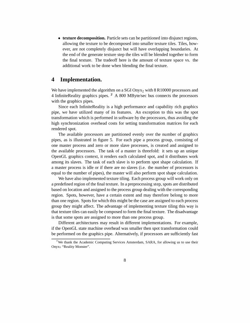
� texture decomposition.Particle sets can be partitioned into disjunct regions,allowing the texture to be decomposed into smaller texture tiles. Tiles, how-ever, are not completely disjunct but will have overlappingboundaries. Atthe end of the generate texture step the tiles will be blendedtogether to formthe final texture. The tradeoff here is the amount of texture space vs. theadditional work to be done when blending the final texture.

4 Implementation.

We have implemented the algorithm on a SGI Onyx2 with 8 R10000 processors and4 InfiniteReality graphics pipes.2 A 800 MByte/sec bus connects the processorswith the graphics pipes.

Since each InfiniteReality is a high performance and capability rich graphicspipe, we have utilized many of its features. An exception to this was the spottransformation which is performed in software by the processors, thus avoiding thehigh synchronization overhead costs for setting transformation matrices for eachrendered spot.

The available processors are partitioned evenly over the number of graphicspipes, as is illustrated in figure 5. For each pipe a process group, consisting ofone master process and zero or more slave processes, is created and assigned tothe available processors. The task of a master is threefold:it sets up an uniqueOpenGL graphics context, it renders each calculated spot, and it distributes workamong its slaves. The task of each slave is to perform spot shape calculation. Ifa master process is idle or if there are no slaves (i.e. the number of processors isequal to the number of pipes), the master will also perform spot shape calculation.

We have also implemented texture tiling. Each process groupwill work only ona predefined region of the final texture. In a preprocessing step, spots are distributedbased on location and assigned to the process group dealing with the correspondingregion. Spots, however, have a certain extent and may therefore belong to morethan one region. Spots for which this might be the case are assigned to each processgroup they might affect. The advantage of implementing texture tiling this way isthat texture tiles can easily be composed to form the final texture. The disadvantageis that some spots are assigned to more than one process group.

Different architectures may result in different implementations. For example,if the OpenGL state machine overhead was smaller then spot transformation couldbe performed on the graphics pipe. Alternatively, if processors are sufficiently fast2We thank the Academic Computing Services Amsterdam, SARA, for allowing us to use theirOnyx2 “Reality Monster”.

8

and the caches are large enough then the texture tiles may be competely generatedby the processor, bypassing the graphics subsystem altogether.

5 Applications.

Using the described implementation, two applications wereselected for perfor-mance measurements: an atmospheric pollution model and a direct numerical sim-ulation of a turbulent flow.

5.1 Atmospheric pollution

In [6], computational steering of an atmospheric pollutionmodel is described. Thegoal is to monitor the evolution of pollutant concentrations while the user can con-trol emission, meteorological and geographical parameters. The output is shown asan animated sequence of images. In [6] arrow plots were used to display the windfields, which we have now replaced with spot noise textures. During animation,the user can now very clearly see the evolution of a pollutantand how it relates tothe flow of the wind field. This relation was much less obvious when using arrowplots.

Figure 6 is a snapshot of the resulting animation, showing a spot noise repre-sentation of the wind field and the pollutantO3 superimposed on it. A rainbowcolormap is used for assigning colors to the pollutant. A mapof Europe is alsodrawn.

The data used is a slice from the three dimensional data set. The data is definedon a regular grid of 53x55 cells. Each texture has a resolution of 512x512 pixelsand consists of 2500 spots. Bent spots were used because of the strong fluctuationsin the wind field. Each spot is represented as a 32x17 mesh deformed by the flowusing stream line integration. The net result is that each texture is generated byapproximately 1.3 million quadrilaterals; i.e. 2500x32x17 vertices.

Discussion. Table 1 shows the results of various hardware configurations. Thetimes stated in the table denote the number of spot noise textures that can be gen-erated per second. Only the time for texture synthesis is given; i.e. steps 2 and3 of the spot noise pipeline. Rows of the table denote 1, 2, 4 and 8 number ofprocessors, respectively. Columns denote 1, 2 and 4 number of graphics pipes.

The following observations can be made:� As suggested in equation 2, using more processors does indeed improve thetexture generation rate, with a maximum of approximately 4 processors per

9

Figure 6: PollutantO3 superimposed on the wind field.

1 2 41 1.02 2.0 2.04 2.8 3.6 3.98 2.7 4.9 5.6

Table 1: Textures per second for atmospheric pollution simulation. Columns de-note the number of graphics pipes. Rows denote the number of processors.

graphics pipe. Using more than 4 processors per pipe does notincreaseperformance.� Increasing the number of graphics pipes will also improve the texture gen-eration rate if and only if there are a sufficient number of processors to keepthe graphics pipes busy.� We would expect a near linear performance speedup in the cases that4nprocessors andn graphics pipes are used.3 However this is not so, due to3We expect, but have not verified, that when using 4 graphics pipes an optimal performance will

be achieved by using 16 processors.

10

the additional overhead caused by blending step (termc equation 2). Thisblending step is done sequentially.� The bandwidth from processor to graphics subsystem is not the limiting fac-tor. At 5.6 textures per second the total bandwidth needed isapproximately116 MBytes/sec for just the raw geometric data, which is wellbelow themaximum of 800 MBytes/sec.� Using a 32x17 mesh to represent each spot will result in very accurate ren-derings. Lower resolution meshes will result in less accurate renderings, butcan increase performance substantially.

5.2 Direct numerical simulation of a turbulent flow

In [7], methods are discussed for direct numerical simulation of turbulent flow. Thegoal of this application is to study the evolution of the vortex shedding behind ablock, the transition from laminar to turbulent flow, and howthese relate to otherphysical phenomena, such as pressure or helicity. The computation and the size ofthe resulting data base is impressive: a few weeks of computing can easily producea few terabytes of data. A data browser is being developed to analyse such scientificdata bases. In contrast to prerecorded video sequences, thedata browser allows theuser to first select visualization mappings and then play through any part of thedata base.

Figure 7 is a snapshot of a slice of the data set. The flow is fromleft to rightand impinges a block placed in the field. One can clearly see the transition fromlaminar to turbulent flow behind the block. Only if the numberof frames per secondexceeds a threshold can the user monitor how the vortices behave over time.

The data used is a slice from the three dimensional data set. The data is definedon a rectilinear grid with a resolution of 278x208 cells. Each texture has a reso-lution of 512x512 pixels and uses 40,000 spots. Bent spots were used because ofthe turbulent nature of the flow in which strong fluctuations for the flow magnitudeand direction occur. Each spot is represented as a mesh with aresolution of 16x3vertices; i.e. resulting in approximately 1.9 million quadrilaterals per texture.

Discussion. Table 2 shows the results of various hardware configurations. Thetimes stated in the table denote the number of spot noise textures that can be gener-ated per second. The numbers given in table 1 are somewhat higher. Although themesh resolution of each spot is higher in the atmospheric example, we have usedmany more spots in this example.

The following observations can be made:

11

Figure 7: Direct numerical simulation of the wake behind a block showing vortexshedding and transition from laminar to turbulent flow.

1 2 41 0.72 1.3 1.34 2.1 2.1 2.48 2.5 3.2 3.5

Table 2: Textures per second for turbulent flow.� The structure of table 2 is very similar to that of table 1. Thenumbers suggestthat optimal performance can be achieved if 4 processors areused to drive agraphics pipe. Using more graphics pipes, without increasing the number ofprocessors, will not improve the texture generation rate.� The amount of data being transported from processors to the graphics pipesis approximately 31.0 megabyte per texture.� 40,000 spots per texture will result in very accurate renderings. Using lessspots will result in less accurate renderings, but can increase performancesubstantially.

12

6 Conclusion

In this paper we described how fast generation of spot noise textures can be achievedfor the visualization of flow fields. By dividing the collection of spots over a num-ber of processors and graphics pipes, near interactive speeds can be achieved. Be-cause spot noise allows variation of parameters, speed can be traded for quality andhigher speeds than presented in the paper are possible.

Visualization algorithms should be designed to utilize thecapabilities of thegraphics subsystem. Different software vs. hardware tradeoffs may arise as theperformance of processors, memory systems, busses and graphics subsystems in-crease.

References

[1] L. Hesselink and T. Delmarcelle. Visualization of vector and tensor data sets.In L.J. Rosenblum et al., editors,Scientific Visualization: Advances and Chal-lenges, pages 419–433. Academic press, 1994.

[2] L. Tucker and P. Woodward. Visualization methods. In P. Messina and T. Ster-ling, editors,System Software and Tools for High Performance Computing En-vironments, pages 109–113. SIAM, 1993.

[3] J.J. van Wijk. Spot noise – texture synthesis for data visualization. InThomas W. Sederberg, editor,Computer Graphics (SIGGRAPH ’91 Proceed-ings), volume 25, pages 263–272, July 1991.

[4] W.C. de Leeuw and J.J. van Wijk. Enhanced spot noise for vector field visual-ization. In G.M. Nielson and D. Silver, editors,Proceedings Visualization ’95,pages 233–239. IEEE Computer Society Press, 1995.

[5] J. Neider, T. Davis, and M. Woo.OpenGL Programming Guide. Addison-Wesley, 1993.

[6] R. van Liere and J.J. van Wijk. Steering smog prediction.In B. Hertzbergerand P. Sloot, editors,Proceedings HPCN ’97, pages 241–252. Springer-Verlag,1997.

[7] R.W.C.P. Verstappen and A.E.P. Veldman. Direct numerical simulation atlower costs.Journal of Mathematical Engineering, June 1997 (to appear).

13