Displaying Satellite Imagery - SSEC

McIDAS-V Tutorial Displaying Satellite Imagery

updated September 2013 (software version 1.4)

McIDAS-V is a free, open source, visualization and data analysis software package that is the next generation in

SSEC's 40-year history of sophisticated McIDAS software packages. McIDAS-V displays weather satellite

(including hyperspectral) and other geophysical data in 2- and 3-dimensions. McIDAS-V can also analyze and

manipulate the data with its powerful mathematical functions. McIDAS-V is built on SSEC's VisAD and

Unidata's IDV libraries, and contains "Bridge" software that enables McIDAS-X users to run their commands

and tasks in the McIDAS-V environment. The functionality of SSEC's HYDRA software package is also being

integrated into McIDAS-V for viewing and analyzing hyperspectral satellite data.

More training materials are available on the McIDAS-V webpage and in the Getting Started chapter of the

McIDAS-V User’s Guide, which is available from the Help menu within McIDAS-V. You will be notified at

the startup of McIDAS-V when new versions are available on the McIDAS-V webpage -

http://www.ssec.wisc.edu/mcidas/software/v/ .

If you encounter an error or would like to request an enhancement, please post it to the McIDAS-V Support

Forums - http://www.ssec.wisc.edu/mcidas/forums/. The forums also provide the opportunity to share

information with other users.

In this McIDAS-V Tutorial, some exercises will be explained using different methods of data access: local data

files, pre-loaded data bundles and real-time access to default remote servers. If you have access to your own

real-time ADDE servers, you may also use those, but be aware that different server configurations may make the

explanations in this document not quite applicable to all data that you may load.

This tutorial assumes that you have McIDAS-V installed on your machine, and that you know how to start

McIDAS-V. If you cannot start McIDAS-V on your machine, you should follow the instructions in the

document entitled McIDAS-V Tutorial – Installation and Introduction.

Terminology

There are two windows displayed when McIDAS-V first starts, the McIDAS-V Main Display (hereafter

Main Display) and the McIDAS-V Data Explorer (hereafter Data Explorer).

The Data Explorer contains three tabs that appear in bold italics throughout this document: Data Sources,

Field Selector, and Layer Controls. Data is selected in the Data Sources tab, loaded into the Field

Selector, displayed in the Main Display, and output is formatted in the Layer Controls.

Menu trees will be listed as a series (e.g. Edit -> Remove -> All Layers and Data Sources).

Mouse clicks will be listed as combinations (e.g. Shift+Left Click+Drag).

http://www.ssec.wisc.edu/mcidas/software/v/

http://www.ssec.wisc.edu/mcidas/forums/

http://www.ssec.wisc.edu/mcidas/forums/

of 16

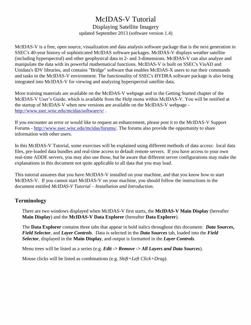
McIDAS-V Tutorial – Displaying Satellite Imagery September 2013 – McIDAS-V version 1.4

Loading Geostationary Satellite Images and Loops

1. Create a local dataset to access the imagery files on your local machine. If you want to load real-time data,

skip to step 3.

a. In the Main Menu Bar in the Main Display window of McIDAS-V, select Tools -> Manage ADDE

Datasets.

b. In the ADDE Data Manager, select File -> New Local Dataset. Enter the following parameters to set

up a dataset with the AREA files provided with this tutorial:

Dataset – MTSAT

Image Type – MTSAT satellite data

Format – McIDAS AREA

Directory – select the <local path>/Data/Satellite/mtsat_dust directory

c. Click Add Dataset. Close the ADDE Data Manager by clicking Ok or select File -> Close.

2. To load the data in this local dataset, follow these steps.

a. Click on the button in the main toolbar to

go to the Data Explorer.

b. From the Data Sources tab, select the Satellite

-> Imagery chooser.

c. Select <LOCAL-DATA> for Server, select

MTSAT for Dataset, click Connect.

d. Choose the MTSAT satellite data Image Type

and select an absolute time of 04:30 UTC.

e. Click Add Source to show the Field Selector.

f. Select 0.73 um VIS Cloud and Surface

Features -> Brightness.

g. Click Create Display. The 04:30 UTC 0.73 μm image is displayed in the Main Display window.

of 16


3. To load real-time data, follow these steps. If you have already loaded the data in step one and two, proceed

to step 4.

a. Click on the button in the Main Toolbar to go to the Data Explorer.

b. Select the Satellite -> Imagery chooser from the Data Sources tab.

c. If you’re using the default servers in McIDAS-V, you can connect to the adde.ucar.edu Server with the

RTIMAGES Dataset.

d. Choose the GE-VIS - GOES-East 0.65 µm Visible Image Type and select an absolute time of 17:45

UTC from the previous day. (This step may be slow, because when choosing absolute times, McIDAS-

V needs to query the ADDE server for all available times.)

e. Click Add Source to show the Field Selector.

f. Select 0.65 um VIS Cloud and Surface Features -> Brightness.

g. Click Create Display. The 17:45 UTC 0.65 μm image is displayed in the Map Display window.

4. Use the zooming and panning controls in the left toolbar to inspect the image.

a. Reset the display projection by clicking on the icon below the zooming buttons on the left toolbar.

b. Turn off the Auto-set Projection option under the Projections menu of the Main Display. When this

option is checked, the projection will automatically change to the native projection of the new layer.

When this option is unchecked, all new layers will be reprojected into the current projection.

5. Edit the maps in the display by using the options in the Layer Controls.

a. Click on Default Background Maps in the Legend to go to the Layer Controls. The map controls will

have two tabs. The first Maps tab lists the available maps, and the second Lat/Lon tab allows the user to

control latitude and longitude lines and labels. At the bottom of both tabs, there is a Position slider that

allows you to control the vertical positioning of the maps in the Main Display.

b. In the Maps tab, you can remove a map, change its visibility, line width, style and color. Use these

options to create your own map display.

c. If you choose, also add latitude and longitude lines and labels in the Lat/Lon tab.

d. To save a map configuration as the default, in the Layer Controls select File -> Default Maps -> Save

as the Default Map Set. The next time you open a new tab, window, or start McIDAS-V, the defaults

will reflect what you selected.

6. Return to the Field Selector to load an infrared image. To load real-time data skip to step 7.

a. Select 10.8 um IR Surface/Cloud-top Temp -> Temperature.

b. Click Create Display.

of 16


7. If you are using real-time data, follow the steps below.

a. Go to the Data Sources tab of the Data Explorer, and using the Satellite -> Imagery chooser with

adde.ucar.edu/RTIMAGES, select the GE-IR – GOES-East 10.7 µm IR Image Type and an absolute

time of 17:45 UTC from the previous day.

b. Click Add Source to show the Field Selector.

c. Select 10.7 um IR Surface/Cloud-top Features -> Temperature. Click Create Display.

8. The 10.8 µm temperature image is overlaid on top of the visible image. To see the visible image, turn off

the top MTSAT Satellite Data (All Bands...) checkbox in the Legend. Turn the image back on and click and

drag the middle mouse button to activate the Cursor/Data Readout option. This option brings up a

latitude, longitude, and data value readout below the display. Since there are two layers in the main display,

there are two different readouts with the appropriate values and units.

9. Change the font and color of the labels on the Main Display.

a. In the Main Display window, choose Edit -> Preferences. Click on Display Window.

b. In the right column under Layer List Properties, change Font to Arial/Plain/14. Change the Color to a

yellow hue. Click OK. Return to the Main Display to see the changes.

10. Notice the labels are the same in the Legend and on the Main Display. This can be customized.

a. Right Click on the top Legend

label, MTSAT satellite data (All

Bands...). (Note: the label will be

different when using real-time

data.)

b. Choose Edit -> Properties... Enter

the following for the Legend

Label and Layer Label:

Legend Label – MTSAT data

– 10.8 um

Layer Label -

%datasourcename% - 10.8 um

%timestamp%

c. Click OK.

11. In the Layer Controls, you can view a histogram of the displayed imagery. Go to the Layer Controls and

click on the Histogram tab for the 10.8 µm image. You can zoom in on a range of data and the display

window will correspondingly change. Left Click+Drag on the histogram to create a box of data to inspect

closer. Note the range of the data in the image display changes to match the range on your histogram. Click

Reset if you wish to return to the original histogram and to the original image.

of 16


12. Create a local dataset to access the FY2E Visible imagery files. To load real-time data skip to step 18.

a. In the Main Display window, select the Tools -> Manage ADDE Datasets menu item.

b. In the ADDE Data Manager, select File -> New Local Dataset, and enter the following parameters:

Dataset – MEGI_VIS

Image Type – FY2E VIS satellite data

Format – McIDAS AREA

Directory – select the <local path>/Data/Satellite/fy2e_vis_megi directory

c. Click Add Dataset.

13. Create a local dataset to access the FY2E Infrared imagery files on your machine.

a. In the ADDE Data Manager, select File -> New Local Dataset, and enter the following parameters:

Dataset – MEGI_IR

Image Type – FY2E IR

Format – McIDAS-AREA

Directory – select the <local path>/Data/Satellite/fy2e_ir_megi directory

b. Click Add Dataset.

14. Close the ADDE Data Manager by clicking Ok or select File -> Close.

a. If using real-time data, skip to step 18.

of 16


15. Create a 4 panel display and change the name of the tab.

a. Select Edit -> Remove -> All Layers and Data Sources.

b. Select File -> New Display Tab -> Map Display -> Four Panels from the main menu to create a 4 panel

tab.

c. Double Click on the “untitled” tab name and enter “FY2E 4-panel” in the entry box and click OK to

change the tab name.

16. Display the FY2E Visible image in the top left panel.

a. By default, the last panel created will be the active panel. The lower right panel will be highlighted with

a default color of blue. Click on the top left panel to activate this panel for the next data load.

b. From the Satellite -> Imagery chooser in the Data Sources tab of the Data Explorer, select <LOCAL-

DATA> for Server, select MEGI_VIS for Dataset, click Connect.

c. Choose the FY2E VIS satellite data Image Type and select a relative time of five most recent images.

Check the Create Preview Image box. This checkbox allows the satellite data to display in the Region

tab of the Field Selector instead of just a map of where the data will be once displayed. Click Add

Source to show the Field Selector.

d. In the Fields panel, select 0.73 um VIS Cloud and Surface Features -> Brightness.

e. Change the centering of the image as well as the image size. The screenshot represents the values to

enter in the Advanced tab.

Under Displays, click on the Advanced tab.

Change the Lat: to 20 and Lon: to 124.

Change the Image Size: to 700 X 1100.

Change the Magnification to -5 X -5.

Click Create Display.

The Magnification of -5 X -5 will reduce the amount of

data downloaded. The data is sampled with every fifth

line and fifth element being sent from the server. Also

note that the number of lines and elements chosen may

not fit into the display window. Zoom out to display all

the pixels requested.

of 16


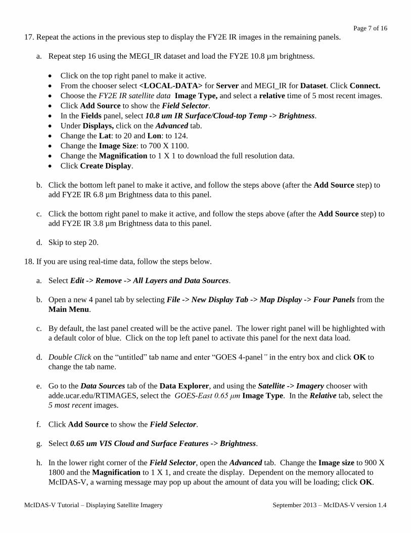
17. Repeat the actions in the previous step to display the FY2E IR images in the remaining panels.

a. Repeat step 16 using the MEGI_IR dataset and load the FY2E 10.8 µm brightness.

Click on the top right panel to make it active.

From the chooser select <LOCAL-DATA> for Server and MEGI_IR for Dataset. Click Connect.

Choose the FY2E IR satellite data Image Type, and select a relative time of 5 most recent images.

Click Add Source to show the Field Selector.

In the Fields panel, select 10.8 um IR Surface/Cloud-top Temp -> Brightness.

Under Displays, click on the Advanced tab.

Change the Lat: to 20 and Lon: to 124.

Change the Image Size: to 700 X 1100.

Change the Magnification to 1 X 1 to download the full resolution data.

Click Create Display.

b. Click the bottom left panel to make it active, and follow the steps above (after the Add Source step) to

add FY2E IR 6.8 µm Brightness data to this panel.

c. Click the bottom right panel to make it active, and follow the steps above (after the Add Source step) to

add FY2E IR 3.8 µm Brightness data to this panel.

d. Skip to step 20.

18. If you are using real-time data, follow the steps below.

a. Select Edit -> Remove -> All Layers and Data Sources.

b. Open a new 4 panel tab by selecting File -> New Display Tab -> Map Display -> Four Panels from the

Main Menu.

c. By default, the last panel created will be the active panel. The lower right panel will be highlighted with

a default color of blue. Click on the top left panel to activate this panel for the next data load.

d. Double Click on the “untitled” tab name and enter “GOES 4-panel” in the entry box and click OK to

change the tab name.

e. Go to the Data Sources tab of the Data Explorer, and using the Satellite -> Imagery chooser with

adde.ucar.edu/RTIMAGES, select the GOES-East 0.65 μm Image Type. In the Relative tab, select the

5 most recent images.

f. Click Add Source to show the Field Selector.

g. Select 0.65 um VIS Cloud and Surface Features -> Brightness.

h. In the lower right corner of the Field Selector, open the Advanced tab. Change the Image size to 900 X

1800 and the Magnification to 1 X 1, and create the display. Dependent on the memory allocated to

McIDAS-V, a warning message may pop up about the amount of data you will be loading; click OK.

of 16


19. Click on the top right panel to make it the active tab. Repeat step 18 using GOES-East 3.9 µm in the top

right panel, GOES-East 10.7 µm in the bottom left panel, and GOES-East 13.3 µm in the bottom right panel.

20. Because the four tabs all have shared views, using the animation controls and zooming and panning in one

panel will make the corresponding changes in the other panels. Observe that this is the case, and then turn

off the share views option in one of the panels.

a. In one of the panels, animate the image loop and zoom in on an interesting weather feature. The other

panels should also begin looping and zoom in on the same geographical location.

b. You may remove one of the panels from updating with the other panels by selecting Projections ->

Share Views in that panels Projections menu.

21. Another feature for real-time data is data polling which allows the data and display to be updated when a

new image exists. Make polling active for all four data sources, have they automatically reload, and check

for new data every 10 minutes.

a. In the Field Selector tab, Right Click on the GOES-East 0.65 µm data source and select Properties.

(Note: The option would function for local datasets if files are updated in the local dataset’s directory.)

b. Under Polling click on the Automatically Reload: Active checkbox. Click on the Reload Displays

checkbox at the bottom of the window.

c. Click Apply and OK. Every 10 minutes (the default polling time) a check will be made for a new image

and if one exists, the satellite loop will be automatically updated in your display.

d. Repeat this step for the remaining three datasets.

Creating RGB images using formulas

22. Create an RGB display from NASA’s high resolution Earth imagery, the Big Blue Marble (BBM) red, green

and blue channels.

a. In the Main Display window, select File -> Open File… and select the

<local path>/Data/Satellite/Sat-RGB-BBM.mcvz file to open. Select Replace session when prompted.

b. Create a new tab via File -> New Display Tab -> Map Display -> One Panel.

23. Define the Red, Green, and Blue channels for your image display.

a. Click on Formulas under the Data Sources listed in the Field Selector.

b. Select Imagery -> Three Color (RGB) Image, and click Create Display.

c. In the Field Selector window, select Big Blue Marble red -> Band 1 as red, Big Blue Marble green ->

Band 1 as green, Big Blue Marble blue -> Band 1 as blue, and click OK.

of 16


24. Save this as a favorite bundle in the toolbar.

a. In the Main Display window, select the File -> Save Favorite… menu item.

b. Under Category select Toolbar and under Name enter in BBM.

c. Make sure the Save as zipped data bundle option is checked and click OK.

d. In the Save Data window choose the Save All Displayed Data option. Click OK. To the right of the

toolbar buttons in the Main Display, there should now be a BBM button.

25. Remove All Layers and Data Sources, and click on the BBM button to see the bundle load. Select Merge

with active tab(s) when prompted.

Problem Sets

The previous examples were intended to give you a general knowledge of how to load and display satellite data.

The problem sets below are intended to introduce you to new topics related to the data, as well as challenge your

knowledge of McIDAS-V. We recommend that you attempt to complete each problem set before looking at the

solutions, which are provided below the problem set.

1. Create a new local dataset for the mudslide files contained in <local path>/Data/Satellite/

fy2e_ir_zhouqu. Load the five most recent FY2E 10.8 µm IR Temperature images from the Zhou Qu

mudslide event and change the enhancement to System -> Inverse Grayscale. Change the range to

enhance the colder clouds, create a color enhancement that has values from 190 to 273 interpolated

between blue and green, and values greater than 273 interpolated to yellow, add a color bar to the image

display window, and save the loop as an animated gif.

2. Create a Parameter default for temperature images so all FY2E Temperature images use the same

enhancement and range as in Problem 1. Then, load several different bands of temperature (10.8 µm, 3.8

µm, etc.) and loop through the different bands.

3. Display a masked loop of FY2E 10.8 µm brightness images from the Zhou Qu mudslide event and

overlay a masked range of 6.8 µm brightness images. Load a data transect for each image and sync them

together. Load a data probe/time series for the 10.8 µm temperature values with the 6.8 µm

temperatures on the same graph. Create a new projection to center the display over China, and change

the display to use this projection.

of 16


Problem Set #1 – Solution

Create a new local dataset for the mudslide files contained in <local path>/Data/Satellite/fy2e_ir_zhouqu.

Load the five most recent FY2E 10.8 µm IR Temperature images from the Zhou Qu mudslide event and change

the enhancement to System -> Inverse Grayscale. Change the range to enhance the colder clouds, create a color

enhancement that has values from 190 to 273 interpolated between blue and green, and values greater than 273

interpolated to yellow, add a color bar to the image display window, and save the loop as an animated gif.

1. Create a local dataset for the mudslide event data and display the 10.8µm temperature data at full resolution.

a. In the ADDE Data Manager, select File -> New Local Dataset. To set up a dataset with the Infrared

AREA files provided with this tutorial enter the following parameters: Dataset: ZQ_IR Image Type:

FY2E IR satellite data Format: McIDAS AREA. Under Directory:, select the

<local path>/Data/Satellite/fy2e_ir_zhouqu. Close the ADDE Data Manager.

b. Select Edit -> Remove -> All Layers and Data Sources.

c. Return to the Data Explorer by clicking on the button in the Main Toolbar.

d. From the Satellite -> Imagery chooser select <LOCAL-DATA> for Server:, select ZQ_IR for

Dataset:, click Connect.

e. Choose the FY2E IR satellite data Image Type and the 5 most recent times. Click Add Source to show

the Field Selector.

f. Select 10.8 µm IR Surface/Cloud-top Temp -> Temperature.

g. Under Displays go to the Advanced tab. Move the magnification sliders to 1x1. Click in the Region

tab. Shift+Left Click in the map display to choose China as the selected display region. Click Create

Display.

2. Right Click on the color table in the Legend and select Change Range.... Edit the values to focus on the

colder clouds. Change the range to 180 to 290 K and click OK.

3. To create a color enhancement, Right Click on the color table and select Edit Color Table. The inverse

gray scale color table will be loaded in with the 180 to 290 K range.

The editor uses “breakpoints” which are used for a number of things: showing the data value at a point along

the color table and changing the colors (fill, interpolation or transparency) directly below the breakpoint.

Breakpoints are indicated along the top of the color legend bar with little triangles and a number.

a. Create a new breakpoint at 273 K by Right Clicking on or near the color table and selecting Add

Breakpoint -> At Data Point. Enter in 273 and click OK. By default, this breakpoint will be active.

The active breakpoint will have a yellow outline around the triangle above the color table.

b. The Color Chooser in the lower half of the editor window allows you to select any possible color. Use

the slider bar to choose a green hue. Once you have chosen a hue, Left Click in the color display to

choose a specific color, which should also update the color of the breakpoint.

of 16


c. Click on the 180 breakpoint to make it active and use the same method to select a dark blue color.

d. Interpolate the colors from 180 to 273 by Right Clicking on the 180 breakpoint and selecting Edit Colors

-> Interpolate -> Right. The enhancement on the images will automatically update.

e. Click on the 290 breakpoint, select a yellow color, and interpolate left to interpolate between 273 and

290.

f. Save the color table as IR Temps in the Satellite category.

i. At the top right of the editor, select Satellite from the Category pull down list.

ii. Select File -> Save As..., enter in IR Temps and click OK. This color table will now show up in the

list of color tables as Satellite -> IR Temps. Close the Color Table Editor.

4. Add a color bar to the top of the image.

a. In the Legend, Right Click on the FY2E IR satellite data and select Edit -> Properties….

b. In the Properties window chose the Color Scale tab. Click the Visible checkbox. Click the Visible and

Show Unit checkboxes for Labels. Change the Font size to 18. Click OK.

5. In the Main Display select View -> Capture -> Movie to bring up the Movie Capture window.

a. Make sure that the Main Display window is not obscured by any other window, including the Data

Explorer and the Movie Capture window.

b. Click the Time Animation button. Each time in the loop will be automatically captured.

c. When the capture is complete, a Save window will pop up. Select “Animated GIF” from the Files of

Type pull down menu, enter in a file name, and click Save.

6. Click Close to close the Movie Capture window.

7. View the movie file in a browser window or movie application.

of 16



Create a Parameter default for temperature images so all FY2E Temperature images use the same enhancement

and range as in Problem 1. Then, load several different bands of temperature (10.8 µm, 3.8 µm, etc.) and loop

through the different bands.

1. From the Main Display window, select Tools -> Parameters -> Defaults from the Main Display to bring

up the Parameter Defaults Editor.

a. Select File -> New Row from the editor menu.

b. Click the double down arrows to the right of the Parameter entry box and select Current Fields ->

FY2E IR (All Bands) -> 37_Band2_TEMP.

c. Modify the Parameter name and replace “37” and “2” with an asterick followed by a period “*.”. The

final result should be: *._Band*._TEMP. These *. symbols act as wildcards, allowing any value to be

in its place.

d. Check the Color Table option and select Satellite -> IR Temps.

e. Check the Range option and enter in a range of 180 to 290.

f. Click OK.

g. Click Close in the Parameter Defaults Editor.

2. Remove All Layers and Data Sources, and from the Satellite -> Imagery chooser select <LOCAL-DATA>

for Server:, select MEGI_IR for Dataset:, click Connect.

a. Choose the FY2E IR satellite data Image Type and select the most recent time. Click Add Source.

b. Select 10.8 µm IR Surface/Cloud-top Temp -> Temperature.

c. Click Create Display. The Typhoon Megi image should have the same range and enhancement as the

Zhou Qu loop did in the previous problem.

3. Repeat using other FY2E Infrared bands with Temperature Data Types with the saved parameter default.

a. Load the 12.0 µm, 6.8 µm and 3.8 µm images in the same display

b. Use the View -> Bring to Front menu option in the Layer Controls for each band to bring the display to

the front.

4. To loop through the different bands, in the Main Display use the View -> Displays -> Visibility Animation

-> On option.

of 16



Display a masked loop of FY2E 10.8 µm temperature images from the Zhou Qu mudslide event and overlay a

masked range of 6.8 µm temperature images. Load a data transect for each image and sync them together. Load

a data probe/time series for the 10.8 µm temperature values with the 6.8 µm temperatures on the same graph.

Create a new projection to center the display over China, and change the display to use this projection.

1. Remove All Layers and Data Sources.

2. Display the FY2E IR data.

a. In the Data Sources tab of the Data Explorer, navigate to the Satellite -> Imagery chooser. Select

<LOCAL-DATA> for the Server, select ZQ_IR for the Dataset, and click Connect.

b. Choose the FY2E IR satellite data Image Type and select the 5 most recent times. Click Add Source.

c. In the Field Selector tab, select Formulas under Data Sources. Under Fields, open the Imagery tree

and select Mask Function. Click Create Display.

d. In the Select Input window, enter the following parameters, then click OK:

comparison – <

cutoff – 240

useNaN – 1

e. In the new Field Selector window, select:

For Field: inputFieldForMask, open and select the ZQ_IR(All Bands)-> 10.8 µm IR

Surface/Cloud-top Temp -> Temperature, and in the Region tab select a region over China.

For Field: displayFieldToBeMasked, open and select the ZQ_IR(All Bands)-> 10.8 µm IR

Surface/Cloud-top Temp -> Temperature , and click OK.

f. Right Click on the color table in the Legend and select Change Range... Edit the values to match the

range of values masked. Change the range to 240 to 180 K and click OK.

g. In the Field Selector tab, select Formulas under Data Sources. Under Fields, open the Imagery tree

and select Mask Within Range. Click Create Display.

h. In the Select Input window, enter the following parameters, then click OK:

minValue – 240

maxValue – 258

useNaN – 1

i. In the new Field Selector window, select:

of 16


For Field: inputFieldForMask, open and select the ZQ_IR(All Bands)-> 6.8 µm IR Mid-level

Water Vapor -> Temperature, and in the Region tab select a region over China (should be selected

from previous step).

For Field: displayFieldToBeMasked, open and select the ZQ_IR(All Bands)-> 6.8 µm IR Mid-

level Water Vapor -> Temperature , and click OK.

j. Right Click on the color table in the Legend and select Change Range... Edit the values to match the

range of values masked. Change the range to 258 to 240 K and click OK. To differentiate from the

other layer, change the color enhancement. Right Click on the color table in the Legend and select

Satellite -> IR Temps.

3. Go back to the Field Selector and select ZQ_IR (All Bands) under Data Sources. Under Fields, select

10.8 µm IR Surface/Cloud-top Temp -> Temperature. Under Displays, select the Data Transect display

type and click Create Display.

4. Repeat the data transect for the 6.8 µm -> Temperature image.

5. Move the red and cyan data transects in the Main Display. Left Click+Drag on the triangle in the center to

move the whole transect. Left Click+Drag on the “+” or “box” to move the endpoints of the transects. The

transect will update in the Layer Controls.

6. In the Legend, Right Click on both transects (under “Cross sections”) and select Edit -> Sharing -> Sharing

On.

7. In the Layer Controls, click on each transect layer and select View -> Undock from Data Explorer to

remove the transects from the Data Explorer.

8. Turn off the FY2E imagery by clicking off the Imagery checkbox in the Legend.

9. Move the WV transect line, keeping it within the bounds of the image. Once you move one of the transects

in the Main Display window, both transects will align and move to the same points.

10. Create a Data Probe/Time Series display of 10.8 µm and 6.8 µm Temperatures.

a. Return to the Field Selector and select the 10.8 µm IR Surface/Cloud-top Temp -> Temperature field.

b. In the Displays panel, select Data Probe/Time Series and click Create Display. The data probe

appears in the Main Display and the time series is in the Layer Controls. Animate the display to see the

data probe time indicator (small black triangle at the top of the graph) and the values in the table below

the graph changing with time.

c. Turn on the FY2E imagery by clicking on the Imagery checkbox in the Legend.

d. In the Main Display move the probe over a cloud with a Left Click+Drag. In the Layer Controls for the

Data Probe, Right Click on the parameter name 37_Band2_TEMP, choose Add Parameter….

of 16


e. In the new Field Selector window choose 6.8 µm IR Mid-level Water Vapor -> Temperature. Click

OK. The cyan 6.8 µm values are added to the graph.

11. China is not a default projection included with McIDAS-V. Create a new projection to center the display

over China.

a. In the Main Display window, select the Tools -> Projections -> Edit Map Projections menu item. This

will open a Projection Manager window.

b. In the Projection Manager window, click the New button to create a new projection.

c. In the Define/Edit Projection window, create a projection over China.

In the Name field, enter China

In the Type field, select Lat/Lon

In the Map panel, Left Click+Drag the black squares to create a bounding box over China.

Click Save

d. Click OK to close the Projection Manager window.

12. Apply your newly-created projection to the display. In the Main Display window, select the Projections ->

Predefined -> China menu item at the bottom of the list.

The display is now centered over China, using the projection created in step 9. This projection will be saved

and can be used in subsequent sessions of McIDAS-V.

of 16


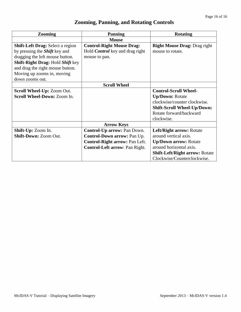
Zooming, Panning, and Rotating Controls

Zooming Panning Rotating

Mouse

Shift-Left Drag: Select a region

by pressing the Shift key and

dragging the left mouse button.

Shift-Right Drag: Hold Shift key

and drag the right mouse button.

Moving up zooms in, moving

down zooms out.

Control-Right Mouse Drag:

Hold Control key and drag right

mouse to pan.

Right Mouse Drag: Drag right

mouse to rotate.

Scroll Wheel

Scroll Wheel-Up: Zoom Out.

Scroll Wheel-Down: Zoom In.

Control-Scroll Wheel-

Up/Down: Rotate

clockwise/counter clockwise.

Shift-Scroll Wheel-Up/Down:

Rotate forward/backward

clockwise.

Arrow Keys

Shift-Up: Zoom In.

Shift-Down: Zoom Out.

Control-Up arrow: Pan Down.

Control-Down arrow: Pan Up.

Control-Right arrow: Pan Left.

Control-Left arrow: Pan Right.

Left/Right arrow: Rotate

around vertical axis.

Up/Down arrow: Rotate

around horizontal axis.

Shift-Left/Right arrow: Rotate

Clockwise/Counterclockwise.

Displaying Satellite Imagery - SSEC

Documents

Transcript of Displaying Satellite Imagery - SSEC