
Dispersants for Crude Oil Spills: Dispersant Behavior Studies
122
Faculty Code: JIB Project Sequence: 1016 Dispersants for Crude Oil Spills: Dispersant Behavior Studies A Major Qualifying Project Report submitted to the faculty of Worcester Polytechnic Institute in partial fulfillment of the requirements for the degree of Bachelor of Science Submitted to: Project Advisor: John Bergendahl, WPI Professor Project Advisor: Nikolaos Kazantzis, WPI Professor Submitted by: Rebecca Diemand Kareem Francis Date: 28 April, 2011 This report represents work of WPI undergraduate students submitted to the faculty as evidence of a degree requirement. WPI routinely publishes these reports on its web site without editorial or peer review. For more information about the projects program at WPI, see http://www.wpi.edu/Academics/Projects.
Transcript of Dispersants for Crude Oil Spills: Dispersant Behavior Studies
Faculty Code: JIB
Project Sequence: 1016
Dispersants for Crude Oil Spills: Dispersant Behavior Studies
A Major Qualifying Project Report submitted to the faculty of Worcester Polytechnic Institute
in partial fulfillment of the requirements for the degree of Bachelor of Science
Submitted to:
Project Advisor: John Bergendahl, WPI Professor
Project Advisor: Nikolaos Kazantzis, WPI Professor
Submitted by:
Rebecca Diemand
Kareem Francis
Date: 28 April, 2011
This report represents work of WPI undergraduate students submitted to the faculty as evidence of a degree requirement. WPI routinely publishes these reports
on its web site without editorial or peer review. For more information about the projects program at WPI, see http://www.wpi.edu/Academics/Projects.

Abstract
The purpose of this study was to experimentally investigate the behavior of the dispersant employed in clean-up efforts to
the Gulf of Mexico affected by the Deepwater Horizon oil spill, namely COREXIT 9500A®. Laboratory results provided
insight into the characteristics of the dispersant and shed light onto some unexpected observations. Analysis of the data
and observations formed several conclusions pertaining to the properties of the dispersant itself as well as the methods of
application involved in the clean-up efforts.

Acknowledgements
This project would not have been possible without the assistance of our advisors Professor John
Bergendahl and Professor Nikolaos Kazantzis as well as the samples of dispersant provided by Marco
Kaltofen.
1
Contents
Abstract…………………………………………………..…………………………….……………i Acknowledgements……………………………………...…………………………………….……..ii Contents……………………………………………………………………………………………..1 List of Tables…………………………………………………………………………………...……3 List of Figures………………………………………………………………………….………....….4 Abbreviations…………………………………………………………………………………….….7 Executive Summary………………………………………………………………………….………8 Chapter 1: Introduction………………………………………………………...……………………11
1.1 Oil Spills……………………………………………………..…………………11 1.1.1 Effects of Oil Spills……………………………..……………….….13 1.1.2 The Exxon Valdez Oil Spill (EVOS)……………..…………………13 1.1.3 Effect of Oil Spills on Plants and Habitats………………………….14 1.1.4 Clean-up Methods for Oil Spills………………………………....…15
1.2 Dispersants……………………………………………..…………………….…20 1.2.1 The Use of COREXIT 9500A & 9527®…………………………....22 1.2.2 Dispersant Influence on Oil………………………………………..22 1.2.3 Existence of Underwater Plumes……………………………….…...23
Chapter 2: Background………………………………………………………………………………25
2.1 Surfactants…………………………...…………………………………….…....26 2.2 Micelle Characterization………………………………………………….……..28
2.2.1 Surface Interactions & Electrical Properties………………….……...28 2.2.2 DLVO Theory………………………………………………..……..29 2.2.3 Ionizable Surface-Group Model…………………………………….29 2.2.4 Van der Waals Forces………………………………………….……29 2.2.5 Double-Layer……………………………………………………….30
2.3 Emulsion Characterization……………………………………………………...31 Chapter 3: Objectives………………………………………………………….……….……………33 Chapter 4: Experimental……………………………………………………………………..………34
4.1 Artificial Sea Water……………………………………………………….……..34 4.2 Turbidity Testing………………………………………………………….…….36 4.3 Light Spectroscopy Testing……………………….……….………………...…..38 4.4 Component Testing………………………………………….……………….…40
4.4.1 2-Butylethanol………………………………….…………………...40 4.4.2 Sodium bis(2-ethylhexyl) Sulfosuccinate………………………….…41
4.5 Disturbing the System with Natural Permutations…………….………………...42 4.5.1 Testing with Sand Particles……………………………………….…42 4.5.2 Testing with Salinity……………………………………….…….….44 4.5.3 Addition of Air Bubbles…………………………………………….45 4.5.4 Testing with Humic Acid…………………………………………...46
4.5.4.1 Humic Acid with Bubble Addition………………………….49 4.5.5 Temperature Adjustment…………………………………………....49 4.5.6 Oil Addition…………………………………………………….…..51
Chapter 5: Results and Analysis……………………...………………………………………………54
5.1 Initial Determinations……………………………………………………….…..54 5.1.1 COREXIT 9500A Concentration……………………………….…..55 5.1.2 Component Analysis…………………………………………….….55
5.1.2.1 2-Butylethanol Addition…………………………………….55
2
5.1.2.2 Sodium bis(2-ethylhexyl) Sulfosuccinate Addition…….…….57 5.2 Salinity Variation Results………………………………………………….…….62
5.2.1 Fifty Percent Sea Water by Volume…………………………….…...62 5.2.2 Seventy-Five Percent Sea Water by Volume………………….……..63 5.2.3 One Hundred Percent Sea Water by Volume………………….……64
5.3 Sand Addition Results…………………………………………….……….……65 5.4 Addition of Air Bubbles……………………………………………..….………72
5.4.1 Salt Water & Deionized Water…………………………..………….72 5.4.2 Salt Water & Humic Acid…………………………….………….….72
5.5 Temperature Variation…………………………………………….……………74 5.5.1 Room Temperature…………………………………..……………..74 5.5.2 Temperature Decrease……………………………………….……...75 5.5.3 Temperature Increase……………………………………….………76 5.5.4 Temperature & COREXIT Volume Comparison………….………..78
5.6 Oil Addition…………………………………………………………….………80 5.6.1 Variation of COREXIT Volume……………………………………80 5.6.2 Variation of Oil Volume………………………………….…………82
Chapter 6: Conclusions………………………………………………………………………………85 Chapter 7: Recommendations………………………………………………………………………..87 References……………………………………………..…………………………………………….89 Appendix A: Experimental Images……………….………………………….………………………93 A.1 Salinity…………………………..…………………………………….…………….…..93 A.2 Sand Addition…….………………………………………………………………...…..96 A.3 Temperature Variation .……………………………………………………………….102 A.4 Oil Additon …………..……………………………………………………………….108 Appendix B: Raw Data Collection ...……………………………………………………………….112

3
List of Tables
Table 1.1 Oil marine pollution from maritime transport procedures……..............................................16
Table 1.2 Fiscal and operational analysis of the Exxon Valdez spill ……………..................................16
Table 1.3 Detailed operational data for dispersants ……...........................................................................18
Table 1.4 List of components of the Dispersant used in the Gulf of Mexico……................................21
Table 2.1 A list of surfactant classifications ……........................................................................................27
Table 4.1 Table of Salts required to make Artificial Seawater……...........................................................34
Table 4.2 Mass of Salt required for synthesis of 2000L of sea water……...............................................35
Table 4.3 Sample of Making Artificial Seawater in 2000L Portions…….................................................35
Table 4.4 Table representing the volume of seawater ratios to pure water ……....................................44
Table 5.1 Comparison of bubbled solutions to initial readings with stirring …….................................72
4
List of Figures Figure 1.1 General location and extent of 2010 Gulf of Mexico oil spill in June. .................................. 11
Figure 1.2 The Site of the Gulf Spill: Closed Areas as of October 22, 2010 ......................................... 12
Figure 1.3 Decaying coral in the Gulf of Mexico, 2010, From the National Oceanic and Atmospheric
Administration ................................................................................................................................................... 14
Figure 1.4 Cleanup of a beach that the Gulf of Mexico contaminated. .................................................. 155
Figure 1.5 Containment boom used during the Gulf of Mexico Oil Spill, 2010 ..................................... 19
Figure 1.6 C-130 Airplane delivering dispersant to the Oil Spill in the Gulf of Mexico, 2010, .......... 200
Figure 1.7 Picture of Kemp’s Ridley turtles in the Gulf of Mexico. ........................................................ 211
Figure 1.8 Mapping of an oil plume in the Gulf of Mexico ........................................................................ 24
Figure 2.1 Plot of oil recoveries versus process aid addition level from the hot water flotation
processing of an oil sand in a continuous pilot plant. Also shown is the correspondence with the zeta
potentials, measured on-line, of emulsified bitumen droplets in the extraction solution .................... 265
Figure 2.2 A graph showing the surface tension trends and micelle formation from monomers as the
dilute surfactant concentration is increased slightly. .................................................................................... 27
Figure 2.3 Various behavioral properties of emulsion droplets before and after CMC ....................... 288
Figure 2.4 Energy diagrams for bitumen-in-water emulsions in the presence of NaCl and CaCl2 ...... 30
Figure 2.5 An illustration of the dynamics and formation of the electric double layer surrounding a
micelle ................................................................................................................................................................ 311
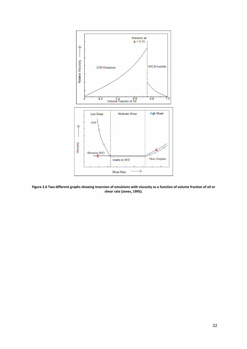
Figure 2.6 Two different graphs showing inversion of emulsions with viscosity as a function of
volume fraction of oil or shear rate. ............................................................................................................... 32
Figure 4.1 Showing Hach 2100N Turbidimeter ........................................................................................ 377
Figure 4.2 Illustrates Empty and fill vials used to test for Turbidity in Hach 2100N Turbidimeter .... 37
Figure 4.3 Side view of 500mL of seawater mixed with 0.5mL and 1.0mL of COREXIT 9500A ...... 37
Figure 4.4 Side and top view of 500mL of Seawater mixed with 1.5mL of COREXIT 9500A ........... 38
Figure 4.5 Side view of 500mL of seawater mixed with 2.0mL of COREXIT 9500A .......................... 38
Figure 4.6 Side view of 500mL of pure water mixed with 1.0mL and 1.5mL of COREXIT 9500A .. 38
Figure 4.7 Side View of 500mL of seawater mixed with 2.0mL and 4.0mL of COREXIT 9500A ..... 38
Figure 4.8 Picture of graph used to evaluate wavelength of greatest absorbance ................................... 39
Figure 4.9 The Cuvette used for the light spectroscopy of the bottom reading of 500mL Seawater
and COREXIT 9500A (1.0mL) ....................................................................................................................... 39
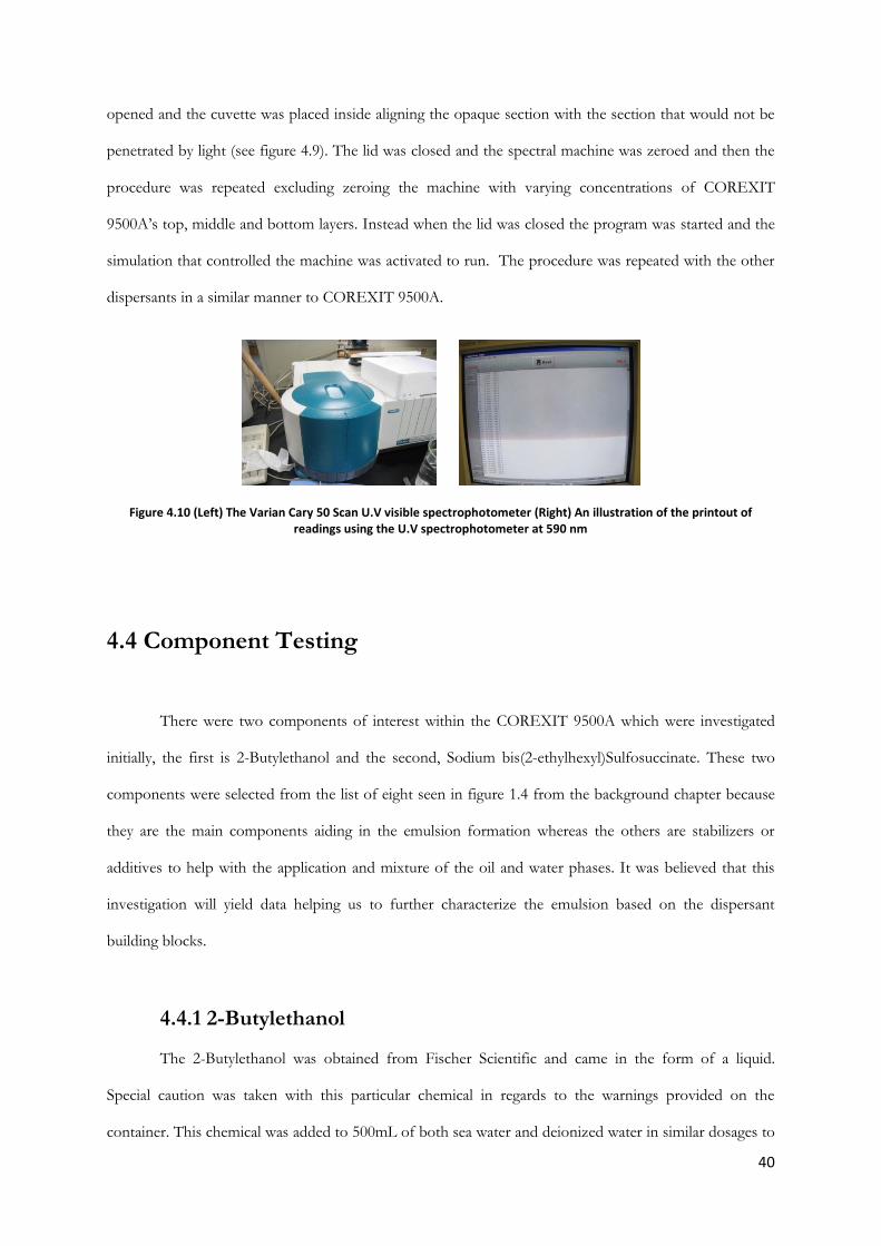
Figure 4.10 (Left) The Varian Cary 50 Scan U.V visible spectrophotometer (Right) An illustration of
the printout of readings using the U.V spectrophotometer at 590 nm ..................................................... 40
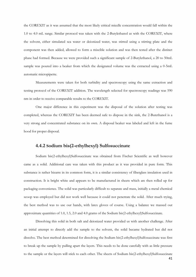
Figure 4.11 Sand used in experiments ordered in decreasing size from left to right and include 0.187
inches, 0.0394, 0.0117 inches, inches and 0.0029 inches. ............................................................................ 43
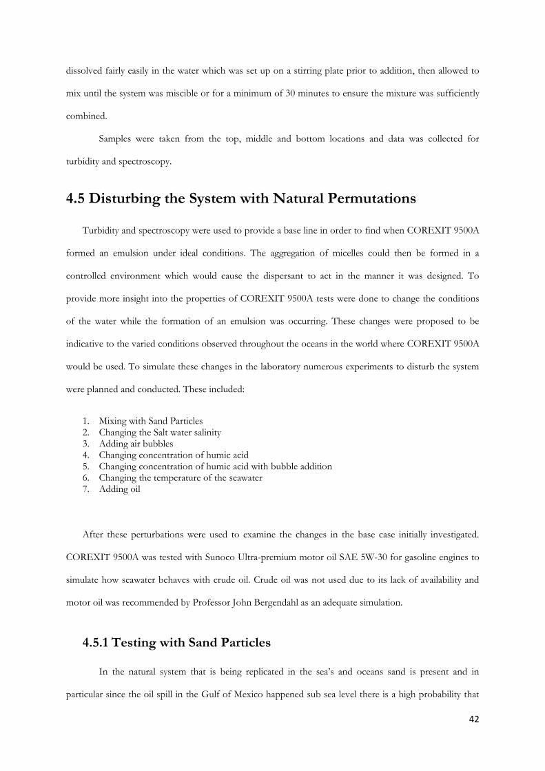
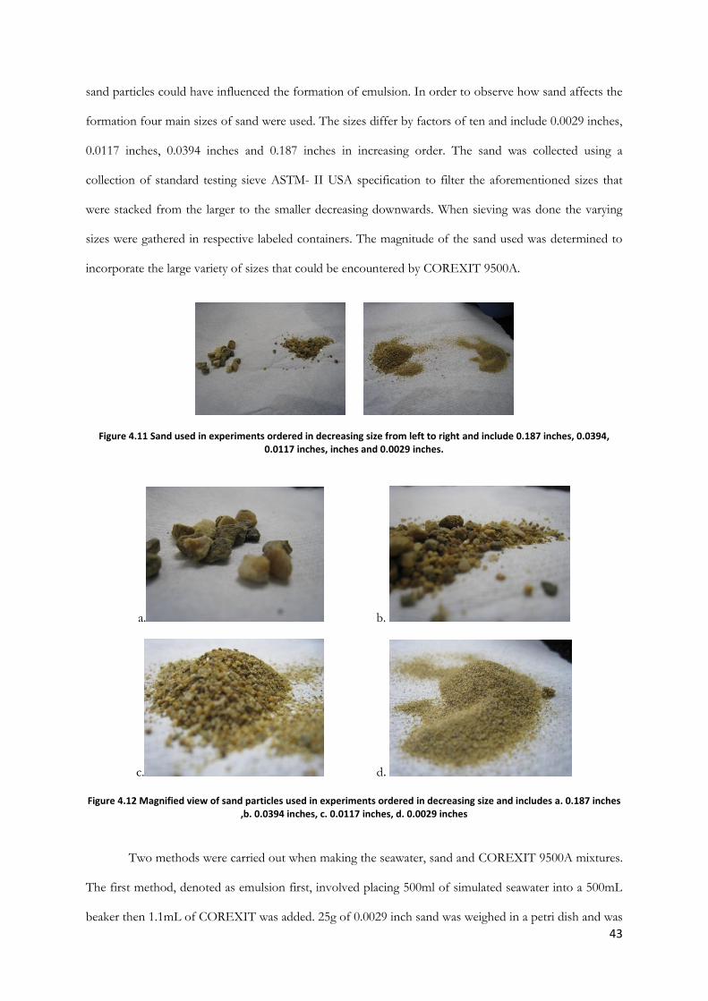
Figure 4.12 Magnified view of sand particles used in experiments ordered in decreasing size and
includesa. 0.187 inches ,b. 0.0394 inches, c. 0.0117 inches, d. 0.0029 inches .......................................... 43
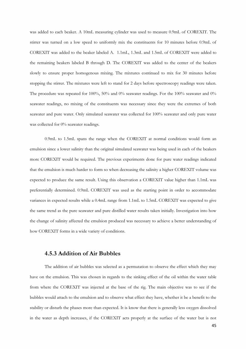
Figure 4.13 Bubbling set up ............................................................................................................................. 46
Figure 4.14 Example of humic acid influence on proton binding in 0.01M of sodium nitrate ............ 47
Figure 4.15 Humic Acid .................................................................................................................................... 48
Figure 4.16 Humic acid at in decreasing concentrations from left to right .............................................. 48
Figure 4.17 (Left) – The COREXIT 9500A in a 50mL beaker (Right) - Sunoco Ultra-premium motor
oil SAE 5W-30 .................................................................................................................................................... 52
Figure 5.1 Increasing volumes of COREXIT 9500A in 500mL of sea water showing CMC ............... 54
5
Figure 5.2 Turbidity results for addition and increase of 2-Butylethanol to 500mL of deionized water
............................................................................................................................................................................... 56
Figure 5.3 Turbidity results for addition and increase of 2-Butylethanol to 500mL of sea water ........ 56
Figure 5.4 Turbidity results for addition and increase of sodium bis(2-ethylhexyl) sulfosuccinate to
500mL of deionized water ................................................................................................................................ 58
Figure 5.5 Turbidity results for addition and increase of sodium bis(2-ethylhexyl) sulfosuccinate to
500mL of sea water............................................................................................................................................ 59
Figure 5.6a Spectroscopy results for addition and increase of sodium bis(2-ethylhexyl) sulfosuccinate
to 500mL of deionized water ........................................................................................................................... 60
Figure 5.6b Magnified view of top and middle layers from figure 5.6a .................................................... 60
Figure 5.7: Spectroscopy results for addition and increase of sodium bis(2-ethylhexyl) sulfosuccinate
to 500mL of sea water ....................................................................................................................................... 61
Figure 5.8 Diagram of absorbance at 590nm of a 50% seawater and 50% pure water mixture as the
volume of COREXIT increases. ..................................................................................................................... 62
Figure 5.9 Diagram of absorbance at 590nm of a 75% seawater and 25% pure water mixture as the
volume of COREXIT increases. ..................................................................................................................... 63
Figure 5.10 Diagram of absorbance at 590nm of a 100% Seawater as the volume of COREXIT
increases. .............................................................................................................................................................. 64
Figure 5.11 Graph of spectroscopy comparing the formation of emulsion when sand added before
and after emulsion formed for top layer. ....................................................................................................... 65
Figure 5.12 Graph of spectroscopy comparing the formation of emulsion when sand added before
and after emulsion formed for middle layer. ................................................................................................. 66
Figure 5.13Graph of spectroscopy comparing the formation of emulsion when sand added before
and after emulsion formed for bottom layer. ................................................................................................ 67
Figure 5.14 Graph of spectroscopy readings varying the size of sand particles for 1.5mL COREXIT
............................................................................................................................................................................... 68
Figure 5.15 Graph of spectroscopy readings varying the size of sand particles for 2.0mL COREXIT.
............................................................................................................................................................................... 69
Figure 5.16 Graph of spectroscopy readings varying the size of sand particles for 2.5mL COREXIT.
............................................................................................................................................................................... 70
Figure 5.17 1.2mL COREXIT in sea water with increasing concentration of humic acid (bubbles &
stirring) ................................................................................................................................................................. 73
Figure 5.18 Graph of Spectroscopy readings for 1.5mL COREXIT 9500A in 500mL of Seawater at
room temperature .............................................................................................................................................. 74
Figure 5.21 Graph of Spectroscopy readings for 2.0mL COREXIT 9500A in 500mL of Seawater at
increased temperature (36 degrees Celsius) ................................................................................................... 77
Figure 5.22 Graph of spectroscopy readings comparing the top layer of emulsions at various
temperatures over time ..................................................................................................................................... 78
Figure 5.23 Graph of spectroscopy readings comparing the middle layer of emulsions at various
temperatures over time ..................................................................................................................................... 79
Figure 5.24 Graph of spectroscopy readings comparing the bottom layer of emulsions at various
temperatures over time ..................................................................................................................................... 79
Figure 5.26 Diagram of turbidity in seawater layer when increasing volumes of COREXIT 9500A is
added to 500mL oil and 450mL Seawater...................................................................................................... 81

6
Figure 5.27 Diagram of absorbance in oil layer when increasing volumes of COREXIT 9500A is
added to 50mL oil and 450mL Seawater ........................................................................................................ 82
Figure 5.28 Diagram of absorbance in seawater layer when increasing volumes of oil is added to
2.0mL COREXIT 9500A and decreasing volumes of Seawater ................................................................ 83

7
List of Abbreviations
ASTM American Society for Testing and Materials CCC Critical Coagulation Concentration
CMC Critical Micelle Concentrations
DLVO Derjaguin, Landau, Verwey and Overbeek
EVOS Exxon Valdez Oil Spill
8
Executive Summary
Background
In April of 2010 the Deepwater Horizon oil rig exploded releasing an estimated 4.9 million barrels
of crude oil into the Gulf of Mexico. The main technique employed to minimize the damage inflicted was
the use of dispersants, mainly COREXIT 9500A®. Dispersants similar to this product have been used in
several other oil spill disasters however little information has been released on the properties and
behavior of these chemicals. Even after observing some of the adverse effects of using this product, no
significant research appears to have been done in the way of investigating why this may be occurring.
Objectives
Our goals for the project include an initial classification and investigation of the emulsion formed
by the dispersant and its apparent properties, specifically focusing on stability. From this point we
furthered our study by experimentally investigating what may adversely affect the stability and relate
observations from the laboratory to those occurring in the environment.
Methodology
A prolonged period of time was spent designing and executing experiments which would reveal
different aspects of the dispersant behavior. Primarily the focus was on creating a consistent and realistic
environment which would appropriately model the natural environment to which the dispersant is
applied. This included the creation of a sea water solution and diagnosing the appropriate volume of
COREXIT necessary to form an emulsion of significant sample size to measure turbidity and absorbance.
Following the familiarization the with dispersant and the emulsion formed, we were able to then advance
to applying permutations to the system in efforts to obtain information on how the dispersant functions
when more variables are introduced which are likely present in the Gulf of Mexico. Measurements to
evaluate the extent of the emulsion development were taken using a turbidimeter and a
9
spectrophotometer. These variations include a decrease in salinity, the addition of particulates including
sand and humic acid, introducing air bubbles to the system, taking data readings from different
temperatures settings and finally the addition of motor oil to the solution. With these influences on the
system we were able to acquire valuable data readings in addition to several observations which will be
explained qualitatively in the proceeding document.
Results and Analysis
Through the experimentation discussed above we were able to determine that temperature has the
most significant impact on the stability of the emulsion. The salinity of the solution appears to have a
significant impact on the micellular formation of the emulsion droplets, allowing for increased
emulsification with increasing salinity. Humic additives, on the other hand, appear to have a negative
effect on the dispersants ability to form an emulsion with sea water; the effect is also magnified when
more gas is dissolved in the system.
Conclusion & Recommendations
Conclusions which arose from the various permutations include the negative effects which both
temperature increase and decrease have on the stability of the emulsion. These results deviate from the
expected behavior of the dispersant and are possibly an explanation to some of the observations made in
the oil contaminated waters. This leads to the belief that the dispersant may not have been formulated for
appropriate use at sub sea level conditions. The second most significant result is the affects the
adjustment of salinity has on the stability of the emulsion phase, this is very telling about the
complications which may ensue when the ocean meets the Mississippi River and the salinity decreases.
Other results are included on the kinetics of the emulsion formation which were not included in our
initial experimental intentions but provided interesting information on how time may affect the
properties of the dispersant under various additions to the solution.
Further recommendations pertain to the extent of experimentation which were available to us.
Our most important recommendation is to create a more realistic simulation of the oil spill environment,
this includes obtaining samples of the waters affected by the oil spill and the addition of crude oil rather

10
than modeling the system with motor oil. Further investigation should be conducted with different and
more advanced technologies to explore other aspects of the dispersant such as surface properties and
bonding abilities.

11
Chapter 1: Introduction
1.1 Oil Spills
The Gulf of Mexico was the site of a massive oil leak that occurred on April 20, 2010 called the
Deepwater Horizon oil spill for the British Petroleum (BP) platform that exploded. The explosion was
the reason for a large fire and released an estimated 780,000m3 (206 million gallons, or 4.9 million barrels)
of oil into the Gulf, (Jackson, J. B. C., et al, 1989).
The area of the spill increased over time to several hundred square kilometers and has since been
reported to have decreased in size. The result of the oil spill caused a ban on fishing in 1180,000 km2 of
the Gulf in May 2010 by the US government, (Jackson, J. B. C., et al, 1989 and Kerr et al., 2010). Many
researchers have since tried to assess the impact of the spill and its future consequences.
Figure 1.1 General location and extent of 2010 Gulf of Mexico oil spill in June.
(Jackson, J. B. C., et al, 1989)
As of November 2010, the amount of oil still in the Gulf is unknown but from studies conducted
by experts in the field an estimated 13%-39% is still present in the Gulf that would hopefully be removed
by evaporation or microbial decomposition. The COREXIT dispersants being used could have
potentially formed oil plumes at 1 km depths that have high concentrations between 1-2 ppm of oil
12
(Jackson, J. B. C., et al, 1989 and Kerr, 2010). The discrepancy of how much oil is currently in the Gulf is
uncertain due to the oil that has gone underwater.
The actual amount of oil in the Gulf is an issue of immense concern because of the effects that
crude product has on the surrounding beaches and marshes. Currently, there are no adequate models to
determine the consequent effects on plant and animal life, residing in both land and sea, the effect on the
local fishing economies in these areas and the general health and well-being of sea food being consumed
by the masses in that area, (Jackson, J. B. C., et al, 1989).
The oil continuously flowed into the Gulf for three months after the initial explosion while
remediation efforts to stop the oil spill were considered. In disasters that occurred around the world, such
as the Chernobyl Ukraine nuclear reactor explosion in 1986, it has been suggested that more negative
effects have resulted from remediation efforts put forth by man-kind, (Davydchuk, 1997 and Cronk et al,
1990) and this may be the case in terms of the Deepwater Horizon oil spill as well. In the case of the
affected waters within the Gulf of Mexico, the nutrients found in the Mississippi River coupled with the
warm water temperatures in the Gulf could improve conditions for the natural “oil eating microbes” that
breakdown oil of low molecular weight, and thus improving the dissipation of oil.
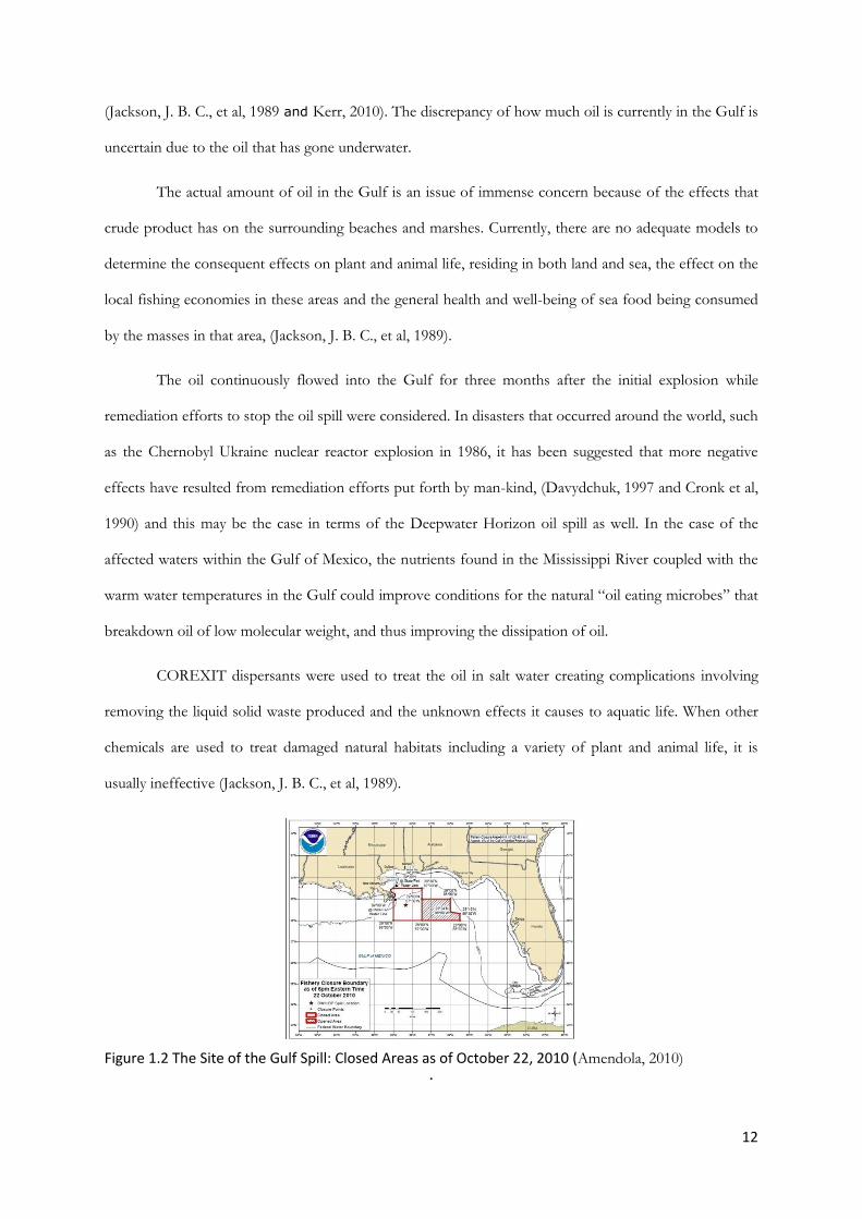
COREXIT dispersants were used to treat the oil in salt water creating complications involving
removing the liquid solid waste produced and the unknown effects it causes to aquatic life. When other
chemicals are used to treat damaged natural habitats including a variety of plant and animal life, it is
usually ineffective (Jackson, J. B. C., et al, 1989).
Figure 1.2 The Site of the Gulf Spill: Closed Areas as of October 22, 2010 (Amendola, 2010) .
13
1.1.1 Effect of Oil Spills
Oil spill occurrences are one of the most environmentally devastating accidents that gain
attention around the world. There have been many accidents reported in places such as India, Norway,
America, England, Spain and Japan, (Campbell et al., 1993, Lyons et al., 1999, Qiao et al., 2002, Chiau,
2005, Balseiro et al., 2005 and Sultan Ayoub Meo et al, 2008).
One example of an oil spill is when the Tasman Spirit Greek oil tanker in 2003 cracked and an
estimated 28,000 tons of crude oil flowed into the sea. When the air pollution was measured after the oil
started to appear onshore it was discovered that 11,000 tons of volatile organic compounds had been
released into the atmosphere, (Sultan Ayoub Meo et al, 2008).
When oil washes onto shore lines it creates a poisonous atmosphere for the people who live
nearby in cities and surrounding areas, (Tasman Spirit oil spill assessment report, 2005). When there is a
crude oil spill in sea water, land effects are sometimes unavoidable and cause coughing, sore throat,
shortness of breath, asthmatic attacks and runny nose. Wildlife such as marine mammals, fish and
seabirds have died as a result of oil spills, (Lyons et al., 1999, Moritam et al., 1999, Carrasco et al., 2006,
and Sultan Ayoub Meo et al, 2008)
1.1.2 The Exxon Valdez Spill (EVOS)
Another glaring example of an oil spill occurred on March 24, 1989, when the Exxon Valdez, a
super tanker, hit Bligh Reef close to Prince William Sound, Alaska, USA. The accident caused 39,000
metric tons of crude oil to come in contact with 3,500 km of shoreline from Kenai, Southwestern
Alaskan peninsulas and Kodiak Island Archipelago’s. The spill started very close to Nearshore, a system
renowned for its aquatic life, (Bowyer, R. Terry, et al. 2003).
Seven years later research conducted at these shorelines indicated that increased numbers of
microbes were still present in areas where the oil remained in sediments, (Braddock et al. 1996). The
trapped oil is still dangerous as potential tidal action and storm could cause the oil to be released back
into the sea. (Braddock et al. 1996). A general trend showing the decline in oil concentration has been
14
found, (Short et al, 1996). “Numerous marine organism were harmed as a result of (EVOS)”, (Bowyer, R.
Terry, et al, 2003).
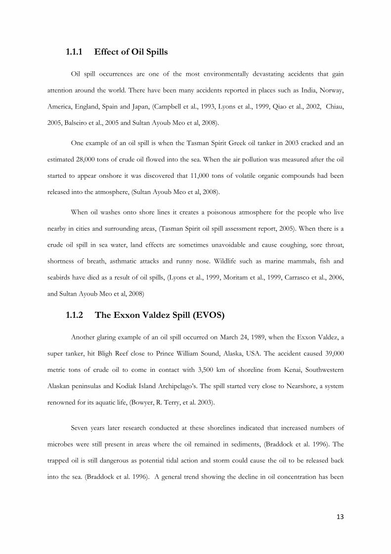
1.1.3 Effect of Oil Spills on Plants and Habitats
Oil Spills also affect coastal marshes that provide a home for numerous wildlife inhabitants and
act as safeguards to the shoreline from intense wave action. Although many experiments have been done,
experts still cannot categorize the various effects that can occur in marsh vegetation. Unknowns about
the effects on vegetation stem from a lack of understanding when oil interacts at the cellular level, (Webb,
1977).
The discharged oil or oil dispersion mixture may reduce habitat use and cause migration patterns
to change, alter the food availability and cause increase deaths among animal populations. The possibility
of oiled plants dying is increased and if this happens the roots would die leading to a higher tendency for
erosion to take place with the loose soil.
Figure 1.3 Decaying coral in the Gulf of Mexico, 2010, From the National Oceanic and Atmospheric Administration (Deeper Insights, 2010)
15
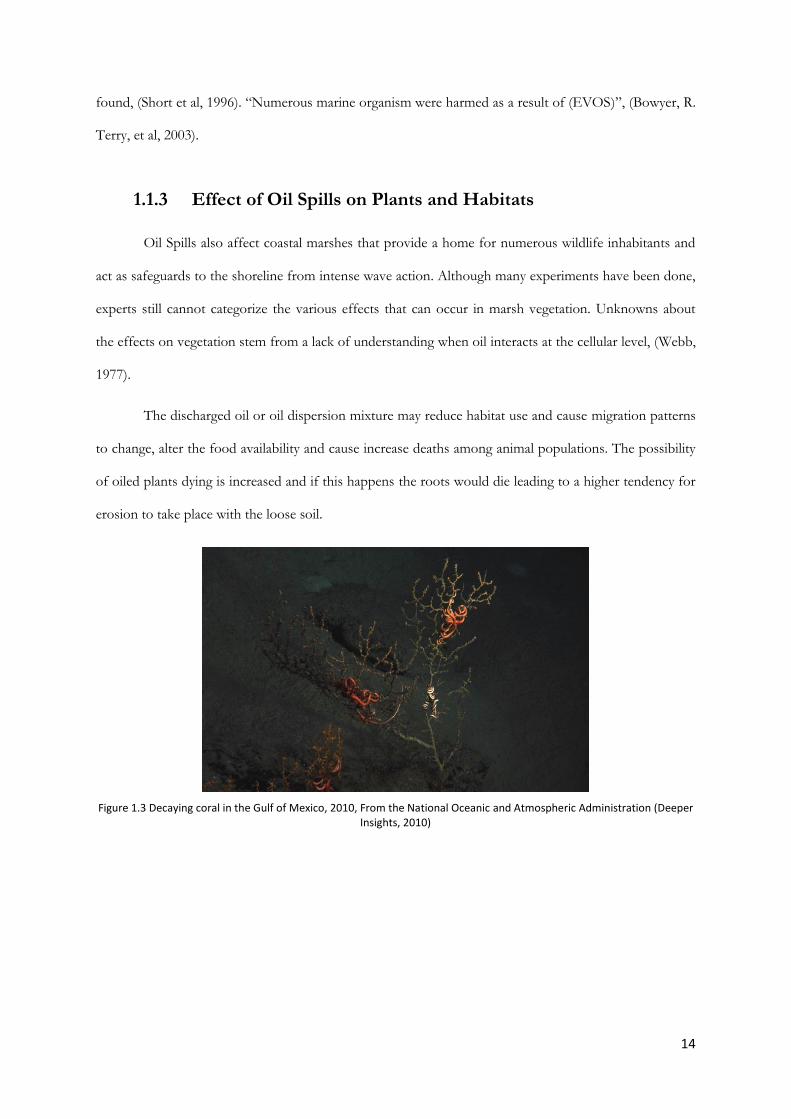
Figure 1.4 Cleanup of a beach that the Gulf of Mexico contaminated (Amazing Images, 2010).
1.1.4 Clean-up Methods for Oil Spills
Cleaning up oil spills is a major issue but terms such as “cleanup” and “countermeasure” are
frequently used and have modified meanings when applied to oil spill cases. The cleanup operation
usually means cleaning up an area that can be accessed and is visible. Examples usually show that the
penetration of oil is much deeper than the corresponding cleanup, as is seen with shore cleanup. Clean up
operations should be well thought out and planned because the operations may cause more damage than
the oil itself. Many large oil spills are caused by marine transport collision, grounding and shipping
operations such as bunkering and loading/unloading. Examples of large cleanups that have taken place
can be seen in disasters such as the “grounding of the Amoco Cadiz (1978), the explosion of Irenes
Serenade (1980), the grounding of the Exxon Valdez (1989) and the grounding of the Sea Empresss
(1996)”, (Nikolaos P. Ventikos et al, 2004).
In the last couple of decades, there have been many advancements and this can be seen in the oil
pollution cases in 1981 compared to 1989.
16
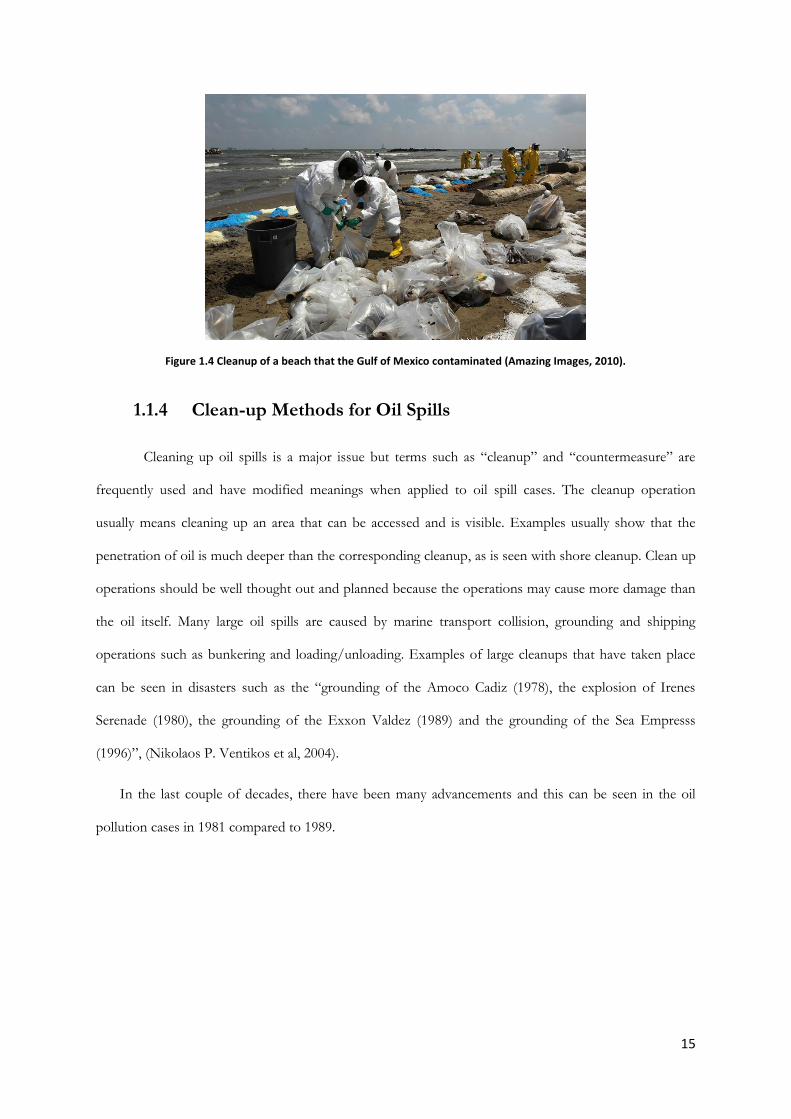
Table 1.1 Oil marine pollution from maritime transport procedures (1981 and 1989), (Nikolaos P. Ventikos et al, 2004).
The response to an oil spill depends mainly on the availability of money which is why proactive
initiatives usually produce the best result. The Exxon Valdez incident caused about $145,000,000,000 in
damages to the environment, leading to the mobilization of 85 aircrafts and 1400 vessels in clean up
efforts. The breakdown of the cost of the Exxon Valdez incident can be seen below, (Nikolaos P.
Ventikos et al, 2004).
Table 1.2 Fiscal and operational analysis of the Exxon Valdez spill (1989)
17
When an oil spill occurs, containing the pollution at the source is the first step. A combination of
recovery, disposal and the containment of oil is performed thereafter. The two main countermeasures
used in oil spills are marine and shore operations, (E. A. Tsocalis et al, 1994). Oil spills have dreadful
implications for people who use the sea as a livelihood, or animal and plant life in the ecosystems
surrounding areas of the spill.
The conventional methods to remove oil from the sea include mechanical clean up, chemical clean
up and natural degradation. Mechanical clean up usually involves containment and recovery of oil
techniques which are synonymous with high economic investment. Chemical methods are focused on
aiding the mechanical process by making the separation easier and natural degradation focuses on
observing nature take its course through wave action.
Some common mechanical cleanup methods are barriers, also known as booms (mechanical barrier),
skimmers which are devices that recover oil and oil and water mixtures from the sea surface. Heavy oil
skimmers are also employed (skimmers that remove high viscosity oils), skimmer vessels (remove oil
from surface) and sorbent materials (recover oil through adhesion), (Nikolaos P. Ventikos et al, 2004).
Chemicals are used to change the characteristic features of the oil, (E. Vergetis, 2004). Dispersants
are the main chemicals used that reduce the interfacial tension between water and oil so that it breaks
down the oil into droplets and quickly disperses into the water. The use of dispersants is a topic of
immense concern because of its potential ecological effects and its relatively short use in real aquatic
environments.
Other chemicals include a mixture of additives such as emulsion breakers (separates water and oil
mixtures), gelling agents, burning agents, neutralizing agents, sinking agents, bioremediation chemicals
(accelerate oil’s natural degradation), viscoelastic additives and herders.
There are several advanced techniques for the removal of oil in sea water that are still considered
experimental. Bioremediation, in-situ burning and cleanmag are examples of these techniques.
Bioremediation uses many different additives to increase natural biodegradation. In-situ burning uses
controlled ignition of an area of oil spilled. It is recommended for large spills and for pollution in the
18
Artic. Cleanmag is a material that has magnetic properties that show a large capacity to absorb oil and
prevent it from polluting a larger area.
The usage of equipment to deliver and to be useful to respond to oil spills depends on variables such
as:
i. Current velocity
ii. Wave height
iii. Viscosity of spilled oil
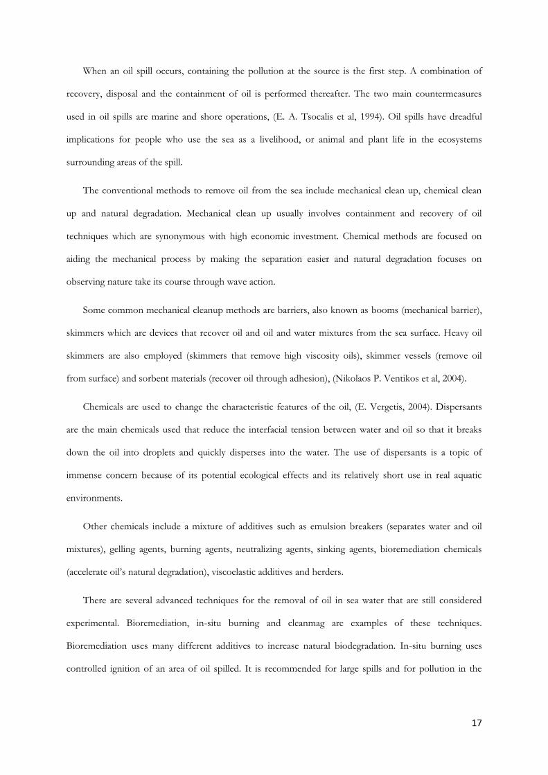
So, depending on criteria such as the current velocity, sea state and the type and weathering
phase of the oil spilled it changes what method can be applied to the oil spill to be effective or even
feasible. The table below shows a preview of what factors are judged for dispersant use to be considered
to be used in the event of an oil spill.
Table 1.3 Detailed operational data for dispersants (K. Lee, 1985)

19
Many different combinations of techniques such as mechanical booms and chemical dispersants
can be used in conjunction if the parameters for both overlap. Therefore both can be used without
concern for one limiting the effectiveness of the other.
Hence, the steps that are followed before choosing a method to apply on an oil spill are as
follows:
i. The state of the sea is recorded (wind velocity, wave height, spilled oil viscosity and
current velocity.
ii. Check what methods of oil spill removal can be used based on the current state of
the sea. Also check what methods can be used in conjunction with each other for
greater removal.
iii. Make a decision on the method to be used at the oil spill site. This decisions should
consider factors such as availability, the capability of the proposed equipment, the
volume of the oil spill, the quality of the available personnel and if there is any
constraints such as non-ideal debris in the oil polluted water.
The most frequently used removal method is mechanical if the conditions permit. The success of the
method selected varies with the deployment time and the type of equipment used to deliver the chosen
method. Some of the methods can damage the coast for example the mechanical use of heavy trucks and
intense vacuums; therefore care has to be taken when choosing the best method. The removal of the oil
from seawater should be beneficial to the environment and not destroy it in the process, (E. Vergetis,
2004).
Figure 1.5 Containment boom used during the Gulf of Mexico Oil Spill (Nichols, 2010).
20
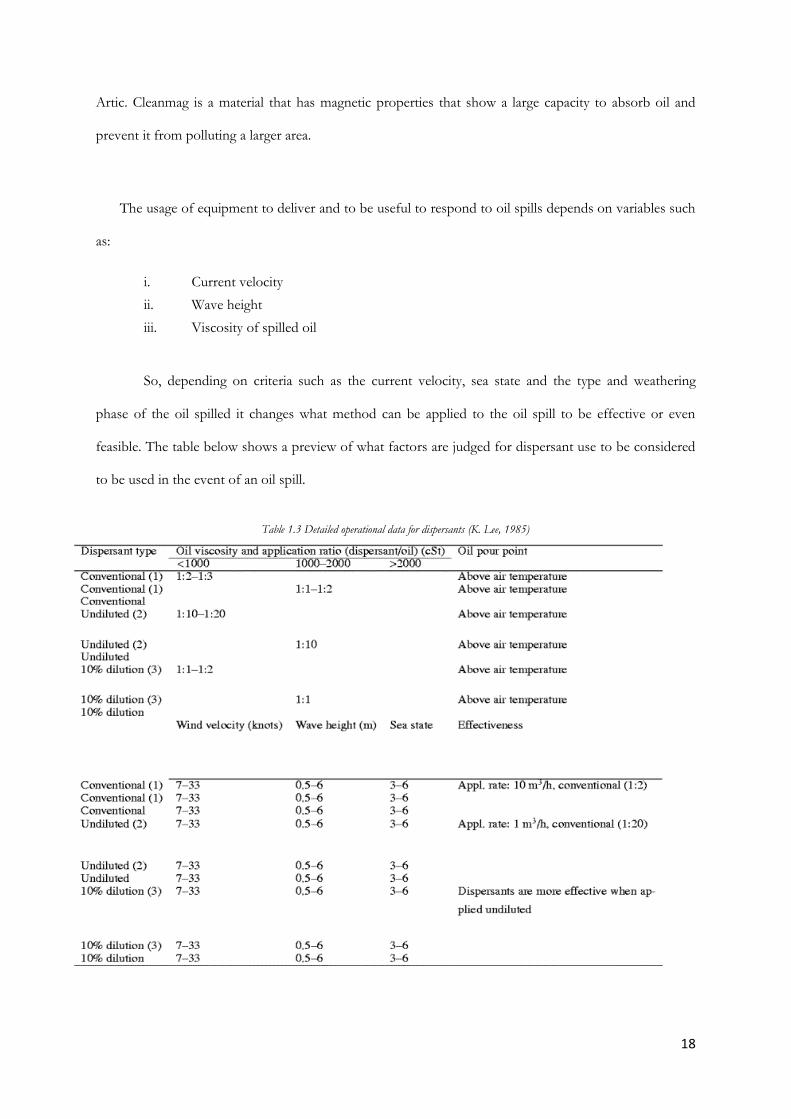
Figure 1.6 C-130 Airplane delivering dispersant to the Oil Spill in the Gulf of Mexico, 2010 (Lehmann, 2010).
1.2 Dispersants
Dispersants started being used in the 1960’s. In the 1970’s and 1980’s, many countries were
reluctant to use dispersants, most likely, due to the negative effects and media coverage that occurred
from the Torrey Canyon spill. Dispersants that were used in the Torrey Canyon spill caused conclusive
environmental damage which perpetuated that the use of dispersants were unsafe. Current dispersants are
said to be much safer by experts, (Etkin, 1999, p. 77), (R. R. Lessard et al, 2000).
A dispersant is similar to a detergent that is used on clothes, instead of removing dirt from a
fabric; it removes oil from sea water surface. It is applied by spraying usually using airplanes onto the site
of the oil slick and this causes the oil to immerse into water column at low concentrations. Dispersants
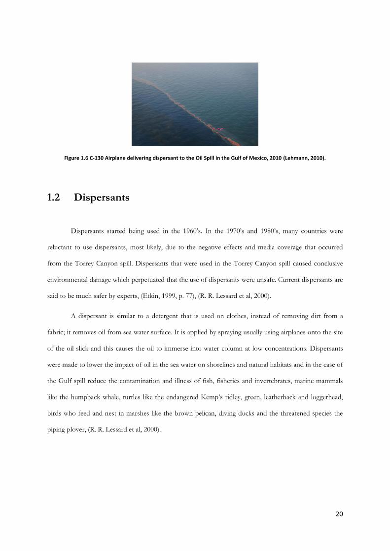
were made to lower the impact of oil in the sea water on shorelines and natural habitats and in the case of
the Gulf spill reduce the contamination and illness of fish, fisheries and invertebrates, marine mammals
like the humpback whale, turtles like the endangered Kemp’s ridley, green, leatherback and loggerhead,
birds who feed and nest in marshes like the brown pelican, diving ducks and the threatened species the
piping plover, (R. R. Lessard et al, 2000).
21
Figure 1.7 Picture of Kemp’s Ridley turtles in the Gulf of Mexico (Witherington, 2010).
“Dispersants are made of surface active agents that are dissolved in one or many solvents”, (R.
R. Lessard et al, 2000). Dispersants are attracted to both oil (lipophilic) and water (hydrophilic) and
dispersants work by decreasing the surface tension between the layers to achieve the alignment of both
the lipophilic and hydrophilic end. Dispersants cause the two immiscible liquids to mix. Dispersants have
to be mixed and the wave action from sea water is what provides this energy when applied to a body of
water. The sea currents cause the oil droplets to disperse into the water column which enables more
aquatic life to survive these disasters, (R. R. Lessard et al, 2000).
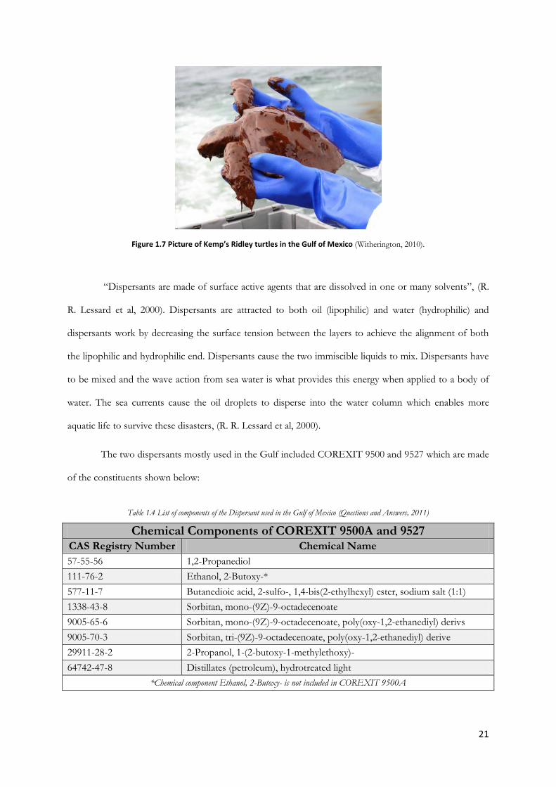
The two dispersants mostly used in the Gulf included COREXIT 9500 and 9527 which are made
of the constituents shown below:
Table 1.4 List of components of the Dispersant used in the Gulf of Mexico (Questions and Answers, 2011)
Chemical Components of COREXIT 9500A and 9527 CAS Registry Number Chemical Name
57-55-56 1,2-Propanediol
111-76-2 Ethanol, 2-Butoxy-*
577-11-7 Butanedioic acid, 2-sulfo-, 1,4-bis(2-ethylhexyl) ester, sodium salt (1:1)
1338-43-8 Sorbitan, mono-(9Z)-9-octadecenoate
9005-65-6 Sorbitan, mono-(9Z)-9-octadecenoate, poly(oxy-1,2-ethanediyl) derivs
9005-70-3 Sorbitan, tri-(9Z)-9-octadecenoate, poly(oxy-1,2-ethanediyl) derive
29911-28-2 2-Propanol, 1-(2-butoxy-1-methylethoxy)-
64742-47-8 Distillates (petroleum), hydrotreated light
*Chemical component Ethanol, 2-Butoxy- is not included in COREXIT 9500A
22
The constituents of the dispersants include two surfactants and an alcohol. The rest of the
additives were included to improve stability of the dispersant or increase the function of the dispersant.
1.2.1 The Use of COREXIT 9500A & 9527®
COREXIT 9527 is a newer dispersant but it has the same low to moderate toxicity and general
effects of COREXIT 9500A, (A. George-Ares et al, 2000) and (Michael M. Singer et al, 1996).
COREXIT 9527 is made by Exxon Production Research Company and it is marketed as a “self-
mixing” concentrate dispersant. It has 3 nonionic and 1 ionic surfactant in a solvent of glycol ether, (K.
Lee, et al, 1985). Field studies have shown that COREXIT 9527 can be distributed using an aircraft.
While COREXIT 9527 is considered a newer dispersant, research has shown that COREXIT
9527 has negative effects on the development and fertilization of sea urchin. There is also research to
suggest that the dispersant also disrupts the formation of marine photo plankton and other bacterivores,
(K. Lee, et al, 1985).
1.2.2 Dispersant Influence on Oil
When a dispersant is added to water it disperses the oil into smaller slicks and eventually sinks
into the water column within hours. The reason for the destabilization of oil in water emulsion is caused
by thermodynamic instability. The dispersant plays a key role in increasing the rate at which the oil is
separated from the water, (Fingas, Merv, 2007)
Processes such as “gravitational forces, surfactant loss to water, and subsequent loss of surfactant
to the water column, creaming, coalescence, flocculation, Ostwald ripening, and sedimentation” result in
the destabilization and resurfacing of oil in water emulsions, (Fingas, Merv, 2007). The application of a
dispersant is pivotal in optimizing its effectiveness to minimize how the oil affects shorelines, mammals
and birds on the water surface and to improve the biodegradation of the oil in the water column.
Currently, research conducted shows no “concrete” data about how effective dispersants added to huge
bodies of water have reduced the shoreline impact, mammal and bird welfare, and improved
biodegradation, (Fingas, Merv, 2007).

23
There is a current debate that exists about the function of some dispersants which cause
inhibition of biodegradation rather than the opposite. No clear correlation of dispersant use being
effective has been produced in modern studies. There are many factors that define how effective a
dispersant can be in the sea and these include the energy of the sea (force of breaking waves),
composition of the oil, the type of oil, the amount, type and temperature of dispersant used, the salinity
and temperature of the water. Though all the previous factors are important, the most essential attributes
in the formation of the emulsions made by the dispersant include the composition of the oil and the sea
energy.
In terms of toxicity, recent tests conclude that the dispersed oil is more toxic than the dispersants
but it was found that the chemically dispersed oil was more toxic than that of physically dispersed oil.
Chemically dispersed oil was found to contain between five to ten times more polycyclic aromatic
hydrocarbons (PAHs) when the water column was tested after using a typical dispersant, (Fingas, Merv,
2007).
Other influences on oil in water dispersion include the way in which the dispersed droplets
especially chemically dispersed interact with high concentrations of sediment. The formation of some oil
with sediment aggregates called oil mineral aggregates (OMAs) have been stable and fallen further into
the depths of the water column, (Fingas, Merv, 2007).
1.2.3 Existence of Underwater Plumes
The dispersant mixed with oil underwater poses a problem as seen in the New York Times article
Gulf of Mexico Oil Spill 2010. The problem occurs because it is unknown, how a large quantity of
dispersant that has been ingested by the water column affects aquatic life. The warm waters of the Gulf
of Mexico and the sea currents moving away from the shore have helped to quell some of the destruction
that could have taken place but as Samantha Joye, a professor of marine sciences from the University of
Georgia highlighted that there is a layer, many centimeters thick on the sea floor about 16 miles from the
point of the leak at the wellhead. Many other independent researchers have also lamented that a large
portion of the oil stays buried on the seafloor. Since these claims have been identified by respected
24
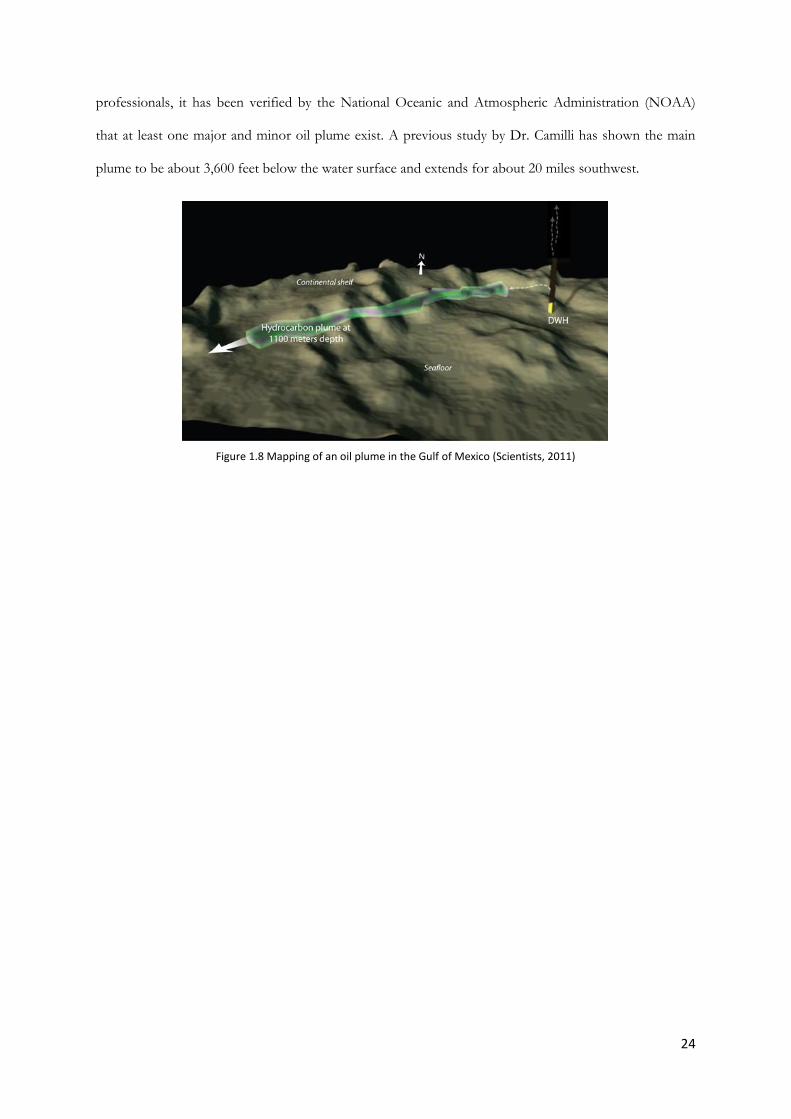
professionals, it has been verified by the National Oceanic and Atmospheric Administration (NOAA)
that at least one major and minor oil plume exist. A previous study by Dr. Camilli has shown the main
plume to be about 3,600 feet below the water surface and extends for about 20 miles southwest.
Figure 1.8 Mapping of an oil plume in the Gulf of Mexico (Scientists, 2011)
25
Chapter 2: Background
There are several topics that were covered in preparation to investigating our project goal. Our
background research was divided into several main areas of interest including characterizing micelles and
emulsions through surface properties, the influence of surfactants and the influences of various additives
to an emulsion surfactant system. This chapter will mostly consist of information which helps to
understand how emulsions are formed on a microscopic level, how these emulsions stabilize and what we
will be able to do test and influence this stability.
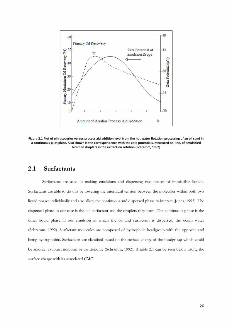
In regards to this project these properties and characteristics are significant because, with
investigation, they may reveal why the dispersant used in the Gulf is not behaving as was expected and
what impact the environment may face as a result. One theory previously used for Enhanced Oil
Recovery (EOR) involved zeta potential of a water-crude-surfactant system. As can be seen in figure 2.1
below, the maximal oil recovery, as a result of the ability for the oil to float, occurs at the same height of
the maximum zeta potential as the concentration of surfactant increases in a bitumen pilot. By observing
the trends seen below, the appropriate amount of surfactant can be estimated based on the zeta potential
of the oil droplets (Schramm, 1992). As we can see, adding infinitely more surfactant will not necessarily
result in more oil recovery and there is no need for excess in the environment, consequences of which
have not been fully investigated.
26
Figure 2.1 Plot of oil recoveries versus process aid addition level from the hot water flotation processing of an oil sand in a continuous pilot plant. Also shown is the correspondence with the zeta potentials, measured on-line, of emulsified
bitumen droplets in the extraction solution (Schramm, 1992)
2.1 Surfactants
Surfactants are used in making emulsions and dispersing two phases of immiscible liquids.
Surfactants are able to do this by lowering the interfacial tension between the molecules within both two
liquid phases individually and also allow the continuous and dispersed phase to interact (Jones, 1995). The
dispersed phase in our case is the oil, surfactant and the droplets they form. The continuous phase is the
other liquid phase in our emulsion in which the oil and surfactant is dispersed, the ocean water
(Schramm, 1992). Surfactant molecules are composed of hydrophilic headgroup with the opposite end
being hydrophobic. Surfactants are classified based on the surface charge of the headgroup which could
be anionic, cationic, nonionic or zwitterionic (Schramm, 1992). A table 2.1 can be seen below listing the
surface charge with its associated CMC.
27
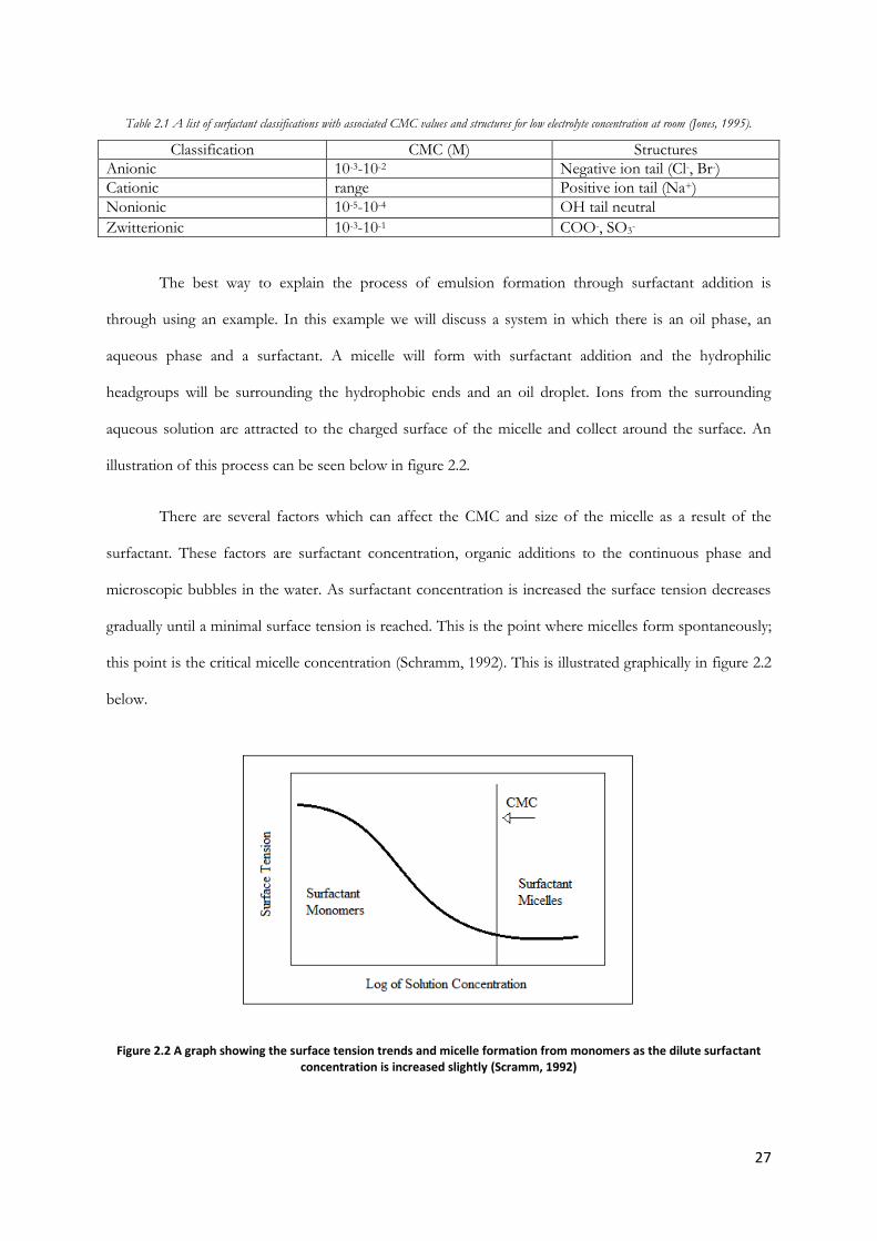
Table 2.1 A list of surfactant classifications with associated CMC values and structures for low electrolyte concentration at room (Jones, 1995).
Classification CMC (M) Structures
Anionic 10-3-10-2 Negative ion tail (Cl-, Br-)
Cationic range Positive ion tail (Na+)
Nonionic 10-5-10-4 OH tail neutral
Zwitterionic 10-3-10-1 COO-, SO3-
The best way to explain the process of emulsion formation through surfactant addition is
through using an example. In this example we will discuss a system in which there is an oil phase, an
aqueous phase and a surfactant. A micelle will form with surfactant addition and the hydrophilic
headgroups will be surrounding the hydrophobic ends and an oil droplet. Ions from the surrounding
aqueous solution are attracted to the charged surface of the micelle and collect around the surface. An
illustration of this process can be seen below in figure 2.2.
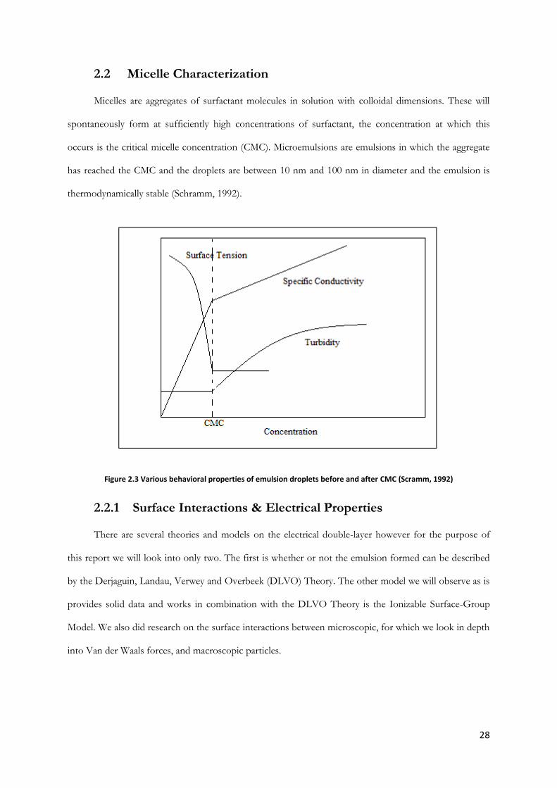
There are several factors which can affect the CMC and size of the micelle as a result of the
surfactant. These factors are surfactant concentration, organic additions to the continuous phase and
microscopic bubbles in the water. As surfactant concentration is increased the surface tension decreases
gradually until a minimal surface tension is reached. This is the point where micelles form spontaneously;
this point is the critical micelle concentration (Schramm, 1992). This is illustrated graphically in figure 2.2
below.
Figure 2.2 A graph showing the surface tension trends and micelle formation from monomers as the dilute surfactant concentration is increased slightly (Scramm, 1992)
28
2.2 Micelle Characterization
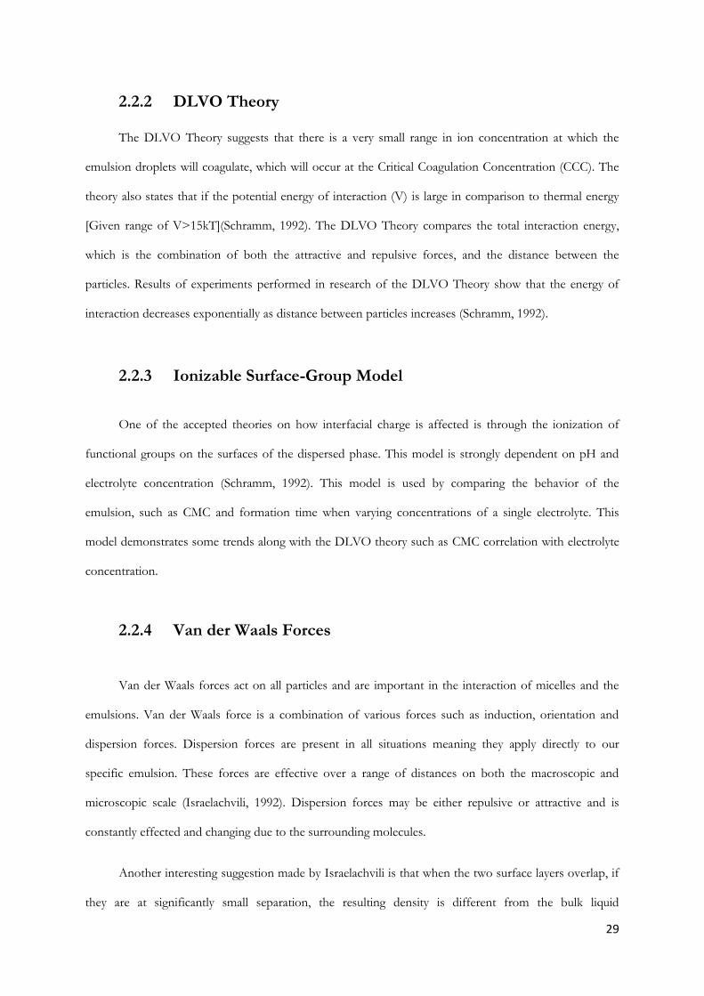
Micelles are aggregates of surfactant molecules in solution with colloidal dimensions. These will
spontaneously form at sufficiently high concentrations of surfactant, the concentration at which this
occurs is the critical micelle concentration (CMC). Microemulsions are emulsions in which the aggregate
has reached the CMC and the droplets are between 10 nm and 100 nm in diameter and the emulsion is
thermodynamically stable (Schramm, 1992).
Figure 2.3 Various behavioral properties of emulsion droplets before and after CMC (Scramm, 1992)
2.2.1 Surface Interactions & Electrical Properties
There are several theories and models on the electrical double-layer however for the purpose of
this report we will look into only two. The first is whether or not the emulsion formed can be described
by the Derjaguin, Landau, Verwey and Overbeek (DLVO) Theory. The other model we will observe as is
provides solid data and works in combination with the DLVO Theory is the Ionizable Surface-Group
Model. We also did research on the surface interactions between microscopic, for which we look in depth
into Van der Waals forces, and macroscopic particles.
29
2.2.2 DLVO Theory The DLVO Theory suggests that there is a very small range in ion concentration at which the
emulsion droplets will coagulate, which will occur at the Critical Coagulation Concentration (CCC). The
theory also states that if the potential energy of interaction (V) is large in comparison to thermal energy
[Given range of V>15kT](Schramm, 1992). The DLVO Theory compares the total interaction energy,
which is the combination of both the attractive and repulsive forces, and the distance between the
particles. Results of experiments performed in research of the DLVO Theory show that the energy of
interaction decreases exponentially as distance between particles increases (Schramm, 1992).
2.2.3 Ionizable Surface-Group Model
One of the accepted theories on how interfacial charge is affected is through the ionization of
functional groups on the surfaces of the dispersed phase. This model is strongly dependent on pH and
electrolyte concentration (Schramm, 1992). This model is used by comparing the behavior of the
emulsion, such as CMC and formation time when varying concentrations of a single electrolyte. This
model demonstrates some trends along with the DLVO theory such as CMC correlation with electrolyte
concentration.
2.2.4 Van der Waals Forces Van der Waals forces act on all particles and are important in the interaction of micelles and the
emulsions. Van der Waals force is a combination of various forces such as induction, orientation and
dispersion forces. Dispersion forces are present in all situations meaning they apply directly to our
specific emulsion. These forces are effective over a range of distances on both the macroscopic and
microscopic scale (Israelachvili, 1992). Dispersion forces may be either repulsive or attractive and is
constantly effected and changing due to the surrounding molecules.
Another interesting suggestion made by Israelachvili is that when the two surface layers overlap, if
they are at significantly small separation, the resulting density is different from the bulk liquid
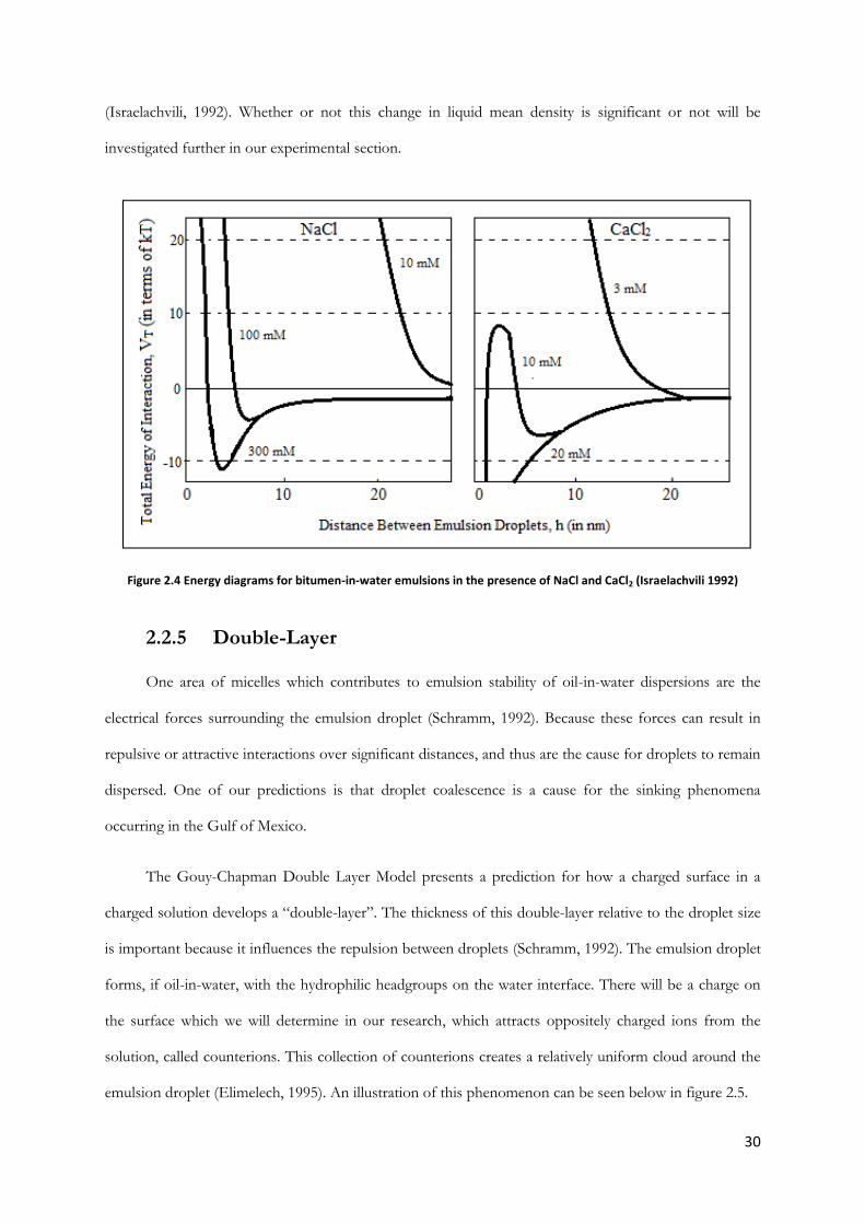
30
(Israelachvili, 1992). Whether or not this change in liquid mean density is significant or not will be
investigated further in our experimental section.
Figure 2.4 Energy diagrams for bitumen-in-water emulsions in the presence of NaCl and CaCl2 (Israelachvili 1992)
2.2.5 Double-Layer
One area of micelles which contributes to emulsion stability of oil-in-water dispersions are the
electrical forces surrounding the emulsion droplet (Schramm, 1992). Because these forces can result in
repulsive or attractive interactions over significant distances, and thus are the cause for droplets to remain
dispersed. One of our predictions is that droplet coalescence is a cause for the sinking phenomena
occurring in the Gulf of Mexico.
The Gouy-Chapman Double Layer Model presents a prediction for how a charged surface in a
charged solution develops a “double-layer”. The thickness of this double-layer relative to the droplet size
is important because it influences the repulsion between droplets (Schramm, 1992). The emulsion droplet
forms, if oil-in-water, with the hydrophilic headgroups on the water interface. There will be a charge on
the surface which we will determine in our research, which attracts oppositely charged ions from the
solution, called counterions. This collection of counterions creates a relatively uniform cloud around the
emulsion droplet (Elimelech, 1995). An illustration of this phenomenon can be seen below in figure 2.5.

31
Figure 2.5 An illustration of the dynamics and formation of the electric double layer surrounding a micelle (Jones, 1995).
2.3 Emulsion Characterization
There are several different sizes of emulsions can form, based on droplet size. There is usually a
range in sizes of emulsion droplets, this distribution can be observed, plotted and skewed to compensate
for changes in stability (Schramm, 1992). In this work, the emulsion had significantly small micelles to be
classified as a microemulsion. In an ideal situation involving an oil, water and surfactant system there are
several different things which occur simultaneously. There will be individual surfactant molecules,
surfactant molecules which have gathered into a micelle and some surfactant molecules will be attached
to an oil droplet with the hydrophobic tail.
Stability has been previously touched on in various sections but here we will discuss how to
create and maintain the stability of an emulsion. The electric double-layer prevents coalescence, high
viscosity of either phase can lead to decreasing the rates of coalescence and creaming. The volume of the
dispersed phase is also an important factor on stability; less of the dispersed phase will reduce collisions
and maintain stability (Schramm, 1992).
32
Figure 2.6 Two different graphs showing inversion of emulsions with viscosity as a function of volume fraction of oil or shear rate (Jones, 1995).
33
Chapter 3: Objectives
The objectives and intentions of experimenting with the COREXIT dispersant are as follows. Each
objective will be investigated with the intentions of determining the basic properties of this emulsion and
to observe emulsion stability along with how it may be negatively influencing the effectiveness of
COREXIT as a dispersant.
1. Characterize the micelles and emulsion as a whole of the COREXIT 9500A emulsion through
experiments such as determining the critical micelle concentration (CMC) and surface properties
which could negatively affect the stability of the emulsion.
2. Create stability experiments on what could adhere to the emulsion and cause it behave differently
than expected. Some of these additions include sand, and other organic particles of various sizes
based on what is found in nature, also observing the effects of adding air bubbles as would be
common in turbulent ocean conditions.
3. Investigate possible ways which the “sinking” phenomena currently seen in the Gulf could be
replicated, based on predictions of what could be occurring based on background knowledge.
34
Chapter 4: Experimental
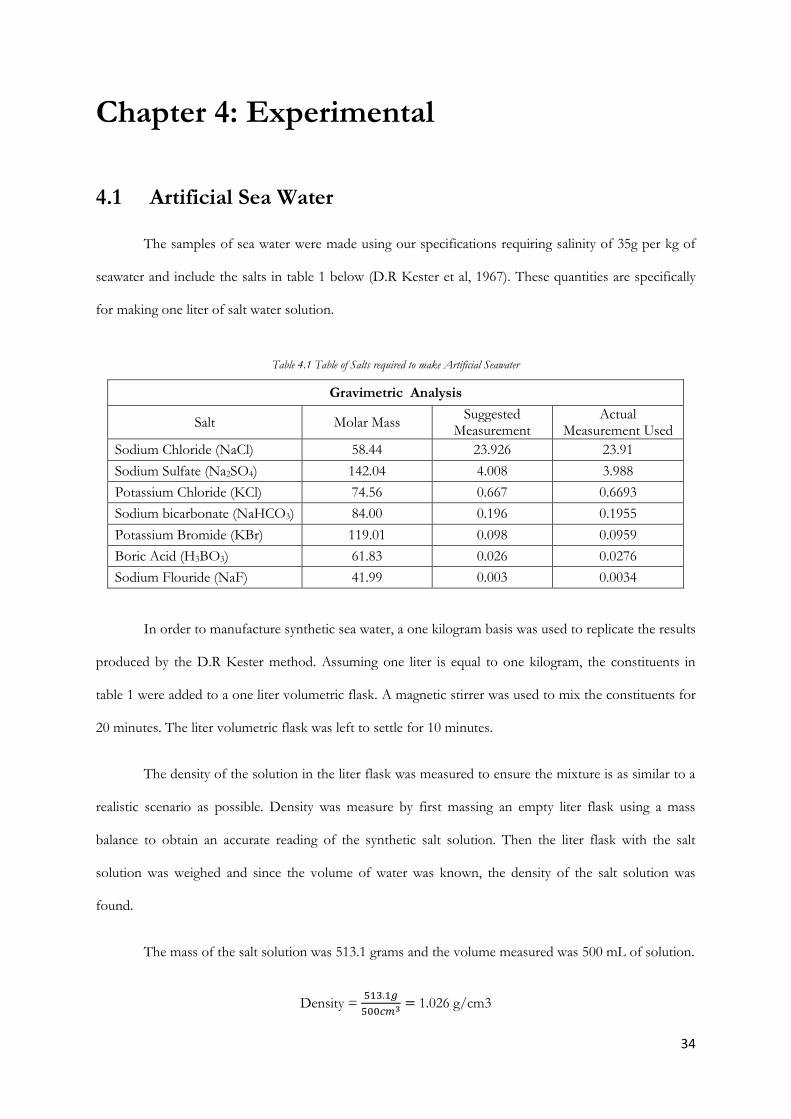
4.1 Artificial Sea Water
The samples of sea water were made using our specifications requiring salinity of 35g per kg of
seawater and include the salts in table 1 below (D.R Kester et al, 1967). These quantities are specifically
for making one liter of salt water solution.
Table 4.1 Table of Salts required to make Artificial Seawater
Gravimetric Analysis
Salt Molar Mass Suggested
Measurement Actual
Measurement Used
Sodium Chloride (NaCl) 58.44 23.926 23.91
Sodium Sulfate (Na2SO4) 142.04 4.008 3.988
Potassium Chloride (KCl) 74.56 0.667 0.6693
Sodium bicarbonate (NaHCO3) 84.00 0.196 0.1955
Potassium Bromide (KBr) 119.01 0.098 0.0959
Boric Acid (H3BO3) 61.83 0.026 0.0276
Sodium Flouride (NaF) 41.99 0.003 0.0034
In order to manufacture synthetic sea water, a one kilogram basis was used to replicate the results
produced by the D.R Kester method. Assuming one liter is equal to one kilogram, the constituents in
table 1 were added to a one liter volumetric flask. A magnetic stirrer was used to mix the constituents for
20 minutes. The liter volumetric flask was left to settle for 10 minutes.
The density of the solution in the liter flask was measured to ensure the mixture is as similar to a
realistic scenario as possible. Density was measure by first massing an empty liter flask using a mass
balance to obtain an accurate reading of the synthetic salt solution. Then the liter flask with the salt
solution was weighed and since the volume of water was known, the density of the salt solution was
found.
The mass of the salt solution was 513.1 grams and the volume measured was 500 mL of solution.
Density =
1.026 g/cm3
35
This was to ensure that the synthetic sea water was the same or close to actual sea water which density is
1.026 grams per cm3 .The density of seawater increases with depth to about 1.028 grams per cm3 and on
the surface it is 1.025 grams per cm3 (D.R Kester et al., 1967).
After the density was confirmed to produce accurate results similar to that of seawater, the mass
of salts needed to make 20 Liters of solution was calculated for further experiments. Then calculated how
much could be made each time using two liter flasks because those were the largest flasks available.
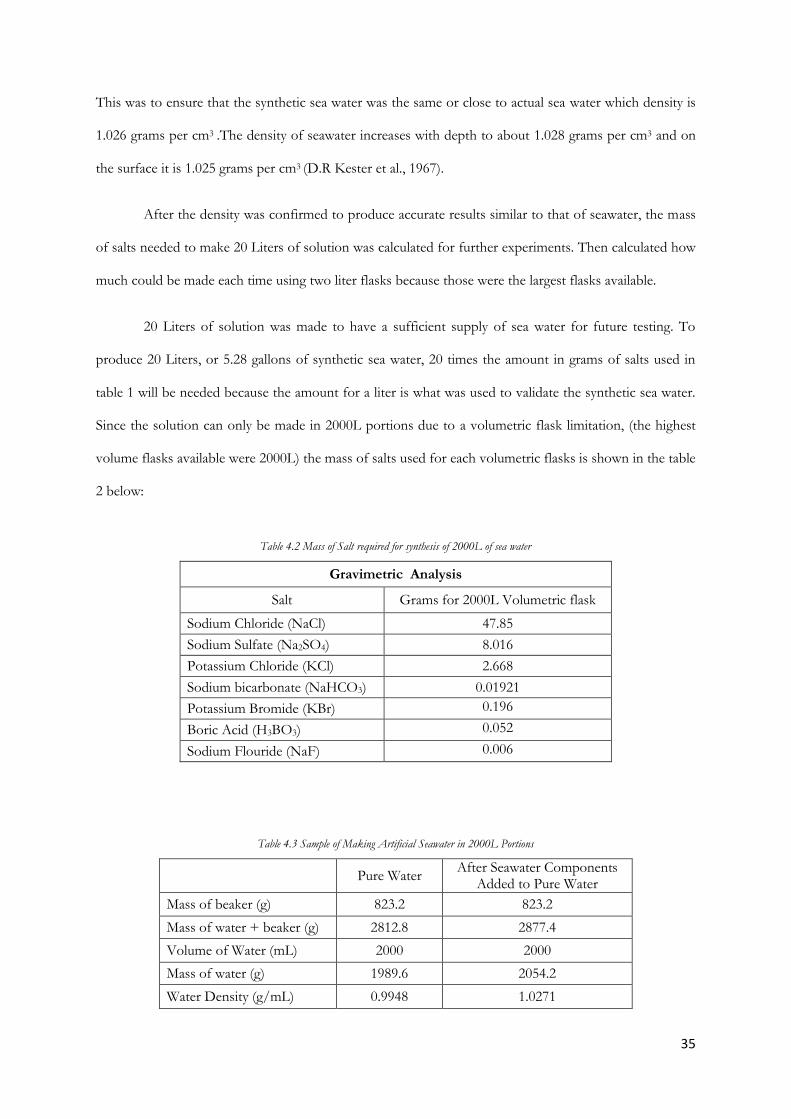
20 Liters of solution was made to have a sufficient supply of sea water for future testing. To
produce 20 Liters, or 5.28 gallons of synthetic sea water, 20 times the amount in grams of salts used in
table 1 will be needed because the amount for a liter is what was used to validate the synthetic sea water.
Since the solution can only be made in 2000L portions due to a volumetric flask limitation, (the highest
volume flasks available were 2000L) the mass of salts used for each volumetric flasks is shown in the table
2 below:
Table 4.2 Mass of Salt required for synthesis of 2000L of sea water
Gravimetric Analysis
Salt Grams for 2000L Volumetric flask
Sodium Chloride (NaCl) 47.85
Sodium Sulfate (Na2SO4) 8.016
Potassium Chloride (KCl) 2.668
Sodium bicarbonate (NaHCO3) 0.01921
Potassium Bromide (KBr) 0.196
Boric Acid (H3BO3) 0.052
Sodium Flouride (NaF) 0.006
Table 4.3 Sample of Making Artificial Seawater in 2000L Portions
Pure Water
After Seawater Components Added to Pure Water
Mass of beaker (g) 823.2 823.2
Mass of water + beaker (g) 2812.8 2877.4
Volume of Water (mL) 2000 2000
Mass of water (g) 1989.6 2054.2
Water Density (g/mL) 0.9948 1.0271
36
In order to manufacture 20L, the procedure for the 2L volumetric flask was done ten times. The
manufactured seawater was collected in a large 20L Nalgene container.
4.2 Turbidity Testing
To test the turbidity of the dispersant and selected surfactant components, COREXIT 9500A, 2-
Butylethanol and sodium bis(2-ethylhexyl) sulfosuccinate in both fresh and simulated sea water. Three
500ml samples of both fresh and sea water were made and each of the three chemicals were added to
both the fresh and sea water. The dispersants were added in a ratio of 1to 50 of oil used to dispersant
used. The ratio was used because it was suggested as the optimum ratio by NALCO© Energy Services in
2006, the creators of the dispersants. See the calculation below for the amount of dispersant added:
Volume of water for sample = 500ml and since ratio is 1:50 oil to dispersant.
We estimated that a thickness of 10% of the volume of water would be the volume of oil,
so in accordance the volume of dispersant was calculated using the following equation
of dispersant.
To produce a range in values of turbidity, varying concentrations of the dispersant and
components were used. Initially four different volumes of 1.0mL, 1.5mL, 2.0mL and 4.0mL of each
chemical was used in order to determine the critical micelle concentration (CMC) which causes an
emulsion to be formed. For an explanation, see Chapter 2: Background.
Steps using the turbidimeter:
1. 1mL of each dispersant or component was added.
2. Each was mixed using a measuring cylinder with a magnetic stirrer to ensure uniformity.
3. The solution was allowed to settle for 20 minutes.
4. The Turbidimeter was turned on, the reading was taken with nothing in the nephlometer, and the
vials were washed with distilled water.
5. Pure water was used to get a baseline reading for the pure water and dispersant mixtures.
Artificial seawater was also used to produce a baseline for the artificial seawater and dispersant
mixtures.
Additional steps:
In each case the seawater samples were tested first then the pure water samples. To test the
seawater and COREXIT 9500A some of the sample from the 500mL measuring cylinder was transferred
37
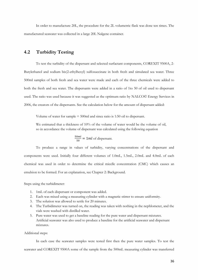
to the turbidimeter vials using a 10mL pipette from the top layer of the vial. The mixture was added to
the turbidimeter vial until the white fill line was reached (see figure 4.2). Opened the turbidimeter lid (see
figure 4.1) and placed the turbidimeter vial inside the turbidimeter and closed the lid. Waited three minute
s for the readings to stabilize before the results were noted. This was repeated for the middle and bottom
layers of the measuring cylinders. The results are shown below in figure 4.1. To ensure validity, identical
turbidity tests were re- performed 24 hours after the initial mixing. The same vial was used to maintain
consistency between readings. The entire procedure was also repeated using 1.5mL, 2.0mL and 4.0mL.
Figure 4.1 Showing Hach 2100N Turbidimeter
Figure 4.2 Illustrates Empty and fill vials used to test for Turbidity in Hach 2100N Turbidimeter
Figure 4.3 Side view of 500mL of seawater mixed with 0.5mL and 1.0mL of COREXIT 9500A
38
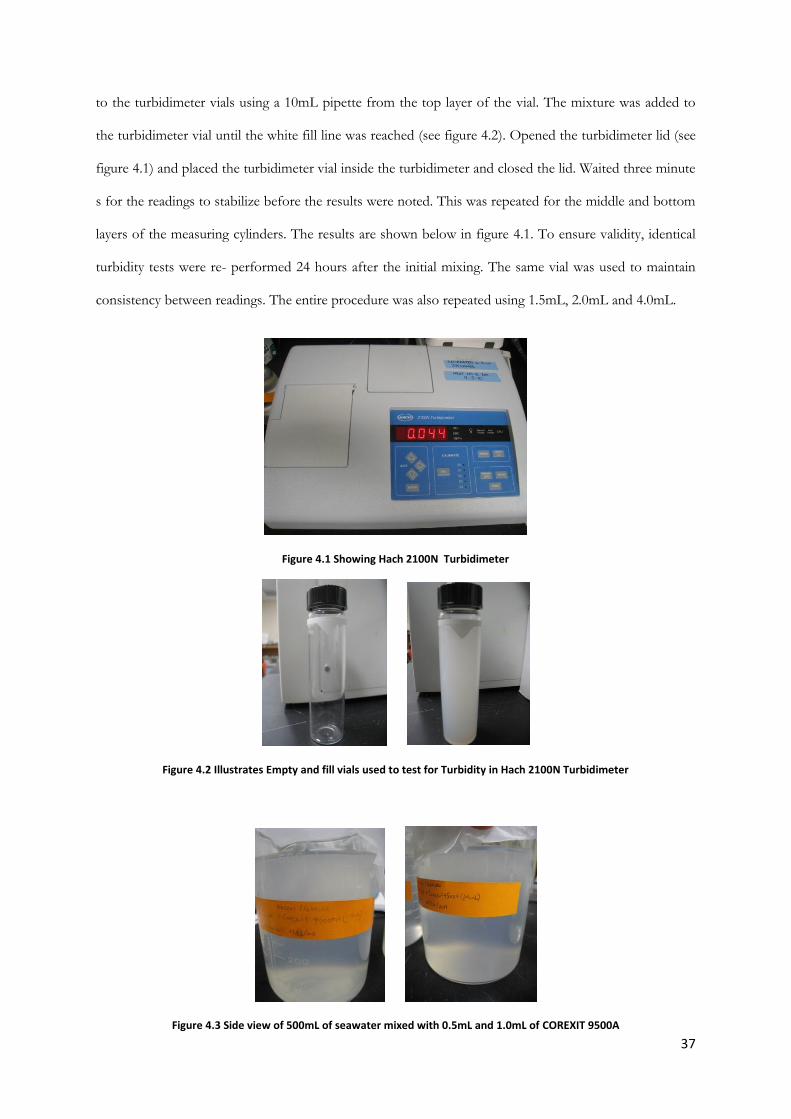
Figure 4.4 Side and top view of 500mL of Seawater mixed with 1.5mL of COREXIT 9500A
Figure 4.5 Side view of 500mL of seawater mixed with 2.0mL of COREXIT 9500A
Figure 4.6 Side view of 500mL of pure water mixed with 1.0mL and 1.5mL of COREXIT 9500A
Figure 4.7 Side View of 500mL of seawater mixed with 2.0mL and 4.0mL of COREXIT 9500A
4.3 Light Spectroscopy Testing
Visible light spectroscopy was also another method that was used to help determine the critical
micelle concentration of the COREXIT 9500A and the other components used.
39
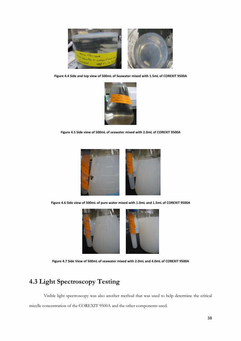
Spectroscopy readings were performed at 590nm because this was the wavelength that had the
most distinct absorbance peak after performing a spectral analysis with the entire spectrum of light using
2.0mL seawater and COREXIT 9500A sample. An example of the entire spectrum of absorbance is
shown in figure 4.8 below. The range of the axes was changed to fit the graphical data represented.
Figure 4.8 Picture of graph used to evaluate wavelength of greatest absorbance
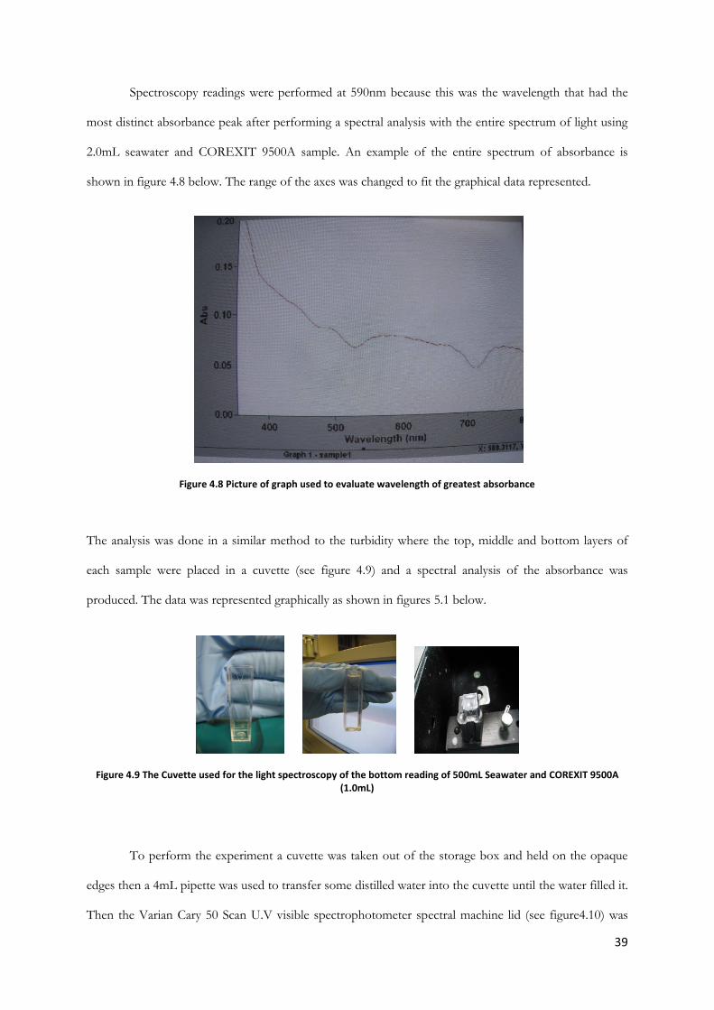
The analysis was done in a similar method to the turbidity where the top, middle and bottom layers of
each sample were placed in a cuvette (see figure 4.9) and a spectral analysis of the absorbance was
produced. The data was represented graphically as shown in figures 5.1 below.
Figure 4.9 The Cuvette used for the light spectroscopy of the bottom reading of 500mL Seawater and COREXIT 9500A (1.0mL)
To perform the experiment a cuvette was taken out of the storage box and held on the opaque
edges then a 4mL pipette was used to transfer some distilled water into the cuvette until the water filled it.
Then the Varian Cary 50 Scan U.V visible spectrophotometer spectral machine lid (see figure4.10) was
40
opened and the cuvette was placed inside aligning the opaque section with the section that would not be
penetrated by light (see figure 4.9). The lid was closed and the spectral machine was zeroed and then the
procedure was repeated excluding zeroing the machine with varying concentrations of COREXIT
9500A’s top, middle and bottom layers. Instead when the lid was closed the program was started and the
simulation that controlled the machine was activated to run. The procedure was repeated with the other
dispersants in a similar manner to COREXIT 9500A.
Figure 4.10 (Left) The Varian Cary 50 Scan U.V visible spectrophotometer (Right) An illustration of the printout of readings using the U.V spectrophotometer at 590 nm
4.4 Component Testing
There were two components of interest within the COREXIT 9500A which were investigated
initially, the first is 2-Butylethanol and the second, Sodium bis(2-ethylhexyl)Sulfosuccinate. These two
components were selected from the list of eight seen in figure 1.4 from the background chapter because
they are the main components aiding in the emulsion formation whereas the others are stabilizers or
additives to help with the application and mixture of the oil and water phases. It was believed that this
investigation will yield data helping us to further characterize the emulsion based on the dispersant
building blocks.
4.4.1 2-Butylethanol The 2-Butylethanol was obtained from Fischer Scientific and came in the form of a liquid.
Special caution was taken with this particular chemical in regards to the warnings provided on the
container. This chemical was added to 500mL of both sea water and deionized water in similar dosages to
41
the COREXIT as it was assumed that the most likely critical micelle concentration would fall within the
1.0 to 4.0 mL range. Similar protocol was taken with the 2-Butylethanol as with the COREXIT, where
the solvent, either simulated sea water or deionized water, was stirred using a stirring plate and the
component was then added, allowed to form a miscible solution and was then tested after the distinct
phase had formed. Because we were provided such a significant sample of 2-Butylethanol, a 20 to 50mL
sample was poured into a beaker from which the designated volume was the extracted using a 0-5mL
automatic micropipette.
Measurements were taken for both turbidity and spectroscopy using the same extraction and
testing protocol of the COREXIT addition. The wavelength selected for spectroscopy readings was 590
nm in order to receive comparable results to the COREXIT.
One major difference in this experiment was the disposal of the solution after testing was
completed, whereas the COREXIT has been deemed safe to dispose in the sink, the 2-Butethanol is a
very strong and concentrated substance on its own. A disposal beaker was labeled and left in the fume
hood for proper disposal.
4.4.2 Sodium bis(2-ethylhexyl) Sulfosuccinate
Sodium bis(2-ethylhexyl)Sulfosuccinate was obtained from Fischer Scientific as well however
came as a solid. Additional care was taken with this product as it was provided in pure form. This
substance is rather bizarre in its common form, it is a similar consistency of fiberglass insulation used in
construction. It is bright white and appears to be manufactured in sheets which are then rolled up for
packaging convenience. The solid was particularly difficult to separate and mass, initially a metal chemical
scoop was employed but did not work well because it could not penetrate the solid. After much trying,
the best method was to use our hands, with latex gloves of course. Using a balance we massed out
approximate quantities of 1.0, 1.5, 2.0 and 4.0 grams of the Sodium bis(2-ethylhexyl)Sulfosuccinate.
Dissolving this solid in both salt and deionized water provided us with another challenge. After
an initial attempt to directly add the sample to the solvent, the solid became hydrated but did not
dissolve. The best method determined for dissolving the Sodium bis(2-ethylhexyl)Sulfosuccinate was first
to break up the sample by pulling apart the layers. This needs to be done carefully with as little pressure
to the sample or the layers will stick to each other. The sheets of Sodium bis(2-ethylhexyl)Sulfosuccinate
42
dissolved fairly easily in the water which was set up on a stirring plate prior to addition, then allowed to
mix until the system was miscible or for a minimum of 30 minutes to ensure the mixture was sufficiently
combined.
Samples were taken from the top, middle and bottom locations and data was collected for
turbidity and spectroscopy.
4.5 Disturbing the System with Natural Permutations
Turbidity and spectroscopy were used to provide a base line in order to find when COREXIT 9500A
formed an emulsion under ideal conditions. The aggregation of micelles could then be formed in a
controlled environment which would cause the dispersant to act in the manner it was designed. To
provide more insight into the properties of COREXIT 9500A tests were done to change the conditions
of the water while the formation of an emulsion was occurring. These changes were proposed to be
indicative to the varied conditions observed throughout the oceans in the world where COREXIT 9500A
would be used. To simulate these changes in the laboratory numerous experiments to disturb the system
were planned and conducted. These included:
1. Mixing with Sand Particles 2. Changing the Salt water salinity 3. Adding air bubbles 4. Changing concentration of humic acid 5. Changing concentration of humic acid with bubble addition 6. Changing the temperature of the seawater 7. Adding oil
After these perturbations were used to examine the changes in the base case initially investigated.
COREXIT 9500A was tested with Sunoco Ultra-premium motor oil SAE 5W-30 for gasoline engines to
simulate how seawater behaves with crude oil. Crude oil was not used due to its lack of availability and
motor oil was recommended by Professor John Bergendahl as an adequate simulation.
4.5.1 Testing with Sand Particles
In the natural system that is being replicated in the sea’s and oceans sand is present and in
particular since the oil spill in the Gulf of Mexico happened sub sea level there is a high probability that
43
sand particles could have influenced the formation of emulsion. In order to observe how sand affects the
formation four main sizes of sand were used. The sizes differ by factors of ten and include 0.0029 inches,
0.0117 inches, 0.0394 inches and 0.187 inches in increasing order. The sand was collected using a
collection of standard testing sieve ASTM- II USA specification to filter the aforementioned sizes that
were stacked from the larger to the smaller decreasing downwards. When sieving was done the varying
sizes were gathered in respective labeled containers. The magnitude of the sand used was determined to
incorporate the large variety of sizes that could be encountered by COREXIT 9500A.
Figure 4.11 Sand used in experiments ordered in decreasing size from left to right and include 0.187 inches, 0.0394, 0.0117 inches, inches and 0.0029 inches.
a. b.
c. d.
Figure 4.12 Magnified view of sand particles used in experiments ordered in decreasing size and includes a. 0.187 inches ,b. 0.0394 inches, c. 0.0117 inches, d. 0.0029 inches
Two methods were carried out when making the seawater, sand and COREXIT 9500A mixtures.
The first method, denoted as emulsion first, involved placing 500ml of simulated seawater into a 500mL
beaker then 1.1mL of COREXIT was added. 25g of 0.0029 inch sand was weighed in a petri dish and was

44
added to the beaker. Paraffin was cut with scissors and placed over the top of the beaker and the beaker
was inverted 10 times then allowed to rest. The sand mixed with the emulsion did not form clearly
enough to make easy observations so the procedure was repeated with 1.5mL, 2.0mL and 2.5mL of
COREXIT for the 0.0029 inch sand. Spectroscopy readings were done after allowing the mixture to settle
for two days. In the second method, denoted as sand first, the main difference is that the sand was added
first to the seawater and then the COREXIT 9500A is added afterwards. The second method follows all
the same steps as the first after the COREXIT 9500A is added and for 0.0029 inches of sand this method
was performed. The procedures for both methods were repeated for 0.0117 inches, 0.0394 inches and
0.187 inches of sand. Turbidity readings were not done because the layer produced for the emulsion
layers were not enough to attain accurate turbidity readings since the volume needed for the
corresponding vials is 30mL.
4.5.2 Testing with Salinity
In natural systems such as the sea and ocean, many lower salinity bodies of water coexist, in
particular estuaries and rivers that are habitats for many different plants and organisms. To replicate how
COREXIT 9500A behaves with these lower salinity conditions, a mixture of pure water and simulated
seawater was combined in varying proportions that included 100% seawater, 75% seawater, 50% seawater
and 0% seawater. Covering this range gives a proper representation of all the bodies of water that have
salinity between these two extremes.
Table 4.4 Table representing the volume of seawater ratios to volume of pure water ratios for the change in salinity experiments
Ratio Volume of Salt Water in
500mL Beaker Volume of Pure water in
500mL Beaker
100% seawater, 0% pure water 500 * 1 = 500mL 500*0 = 0mL
75% seawater, 25% pure water 500 * 0.75 = 375mL 500 * 0.25 = 125mL
50% seawater, 50% pure water 500 * 0.50 = 250mL 500 * 0.50 = 250mL
25% seawater, 75% pure water 500 * 0.25 = 125mL 500 * 0.75 = 375mL
0% seawater, 100% pure water 500 * 0 = 0mL 500 * 1 = 500mL
Four 500mL beakers were labeled A through D. 375mL of simulated seawater was collected four
times in four separate 500mL beakers then 125mL of pure water was added to the beakers for the 75%
seawater ratio experiments. The 500mL beakers were put on magnetic stirrers and a magnetic stirrer bar
45
was added to each beaker. A 10mL measuring cylinder was used to measure 0.9mL of COREXIT. The
stirrer was turned on a low speed to uniformly mix the constituents for 10 minutes before 0.9mL of
COREXIT was added to the beaker labeled A. 1.1mL, 1.3mL and 1.5mL of COREXIT were added to
the remaining beakers labeled B through D. The COREXIT was added to the center of the beakers
slowly to ensure proper homogenous mixing. The mixtures continued to mix for 30 minutes before
stopping the stirrer. The mixtures were left to stand for 2 days before spectroscopy readings were taken.
The procedure was repeated for 100%, 50% and 0% seawater readings. For the 100% seawater and 0%
seawater readings, no mixing of the constituents was necessary since they were the extremes of both
seawater and pure water. Only simulated seawater was collected for 100% seawater and only pure water
was collected for 0% seawater readings.
0.9mL to 1.5mL spans the range when the COREXIT at normal conditions would form an
emulsion since a lower salinity than the original simulated seawater was being used in each of the beakers
more COREXIT would be required. The previous experiments done for pure water readings indicated
that the emulsion is much harder to form so when decreasing the salinity a higher COREXIT volume was
expected to produce the same result. Using this observation a COREXIT value higher than 1.1mL was
preferentially determined. 0.9mL COREXIT was used as the starting point in order to accommodate
variances in expected results while a 0.4mL range from 1.1mL to 1.5mL COREXIT was expected to give
the same trend as the pure seawater and pure distilled water results taken initially. Investigation into how
the change of salinity affected the emulsion produced was necessary to achieve a better understanding of
how COREXIT forms in a wide variety of conditions.
4.5.3 Addition of Air Bubbles The addition of air bubbles was selected as a permutation to observe the effect which they may
have on the emulsion. This was chosen in regards to the sinking effect of the oil within the water table
from where the COREXIT was injected at the base of the rig. The main objective was to see if the
bubbles would attach to the emulsion and to observe what effect they have, whether it be a benefit to the
stability or disturb the phases more than expected. It is know that there is generally less oxygen dissolved
in the water as depth increases, if the COREXIT acts properly at the surface of the water but is not
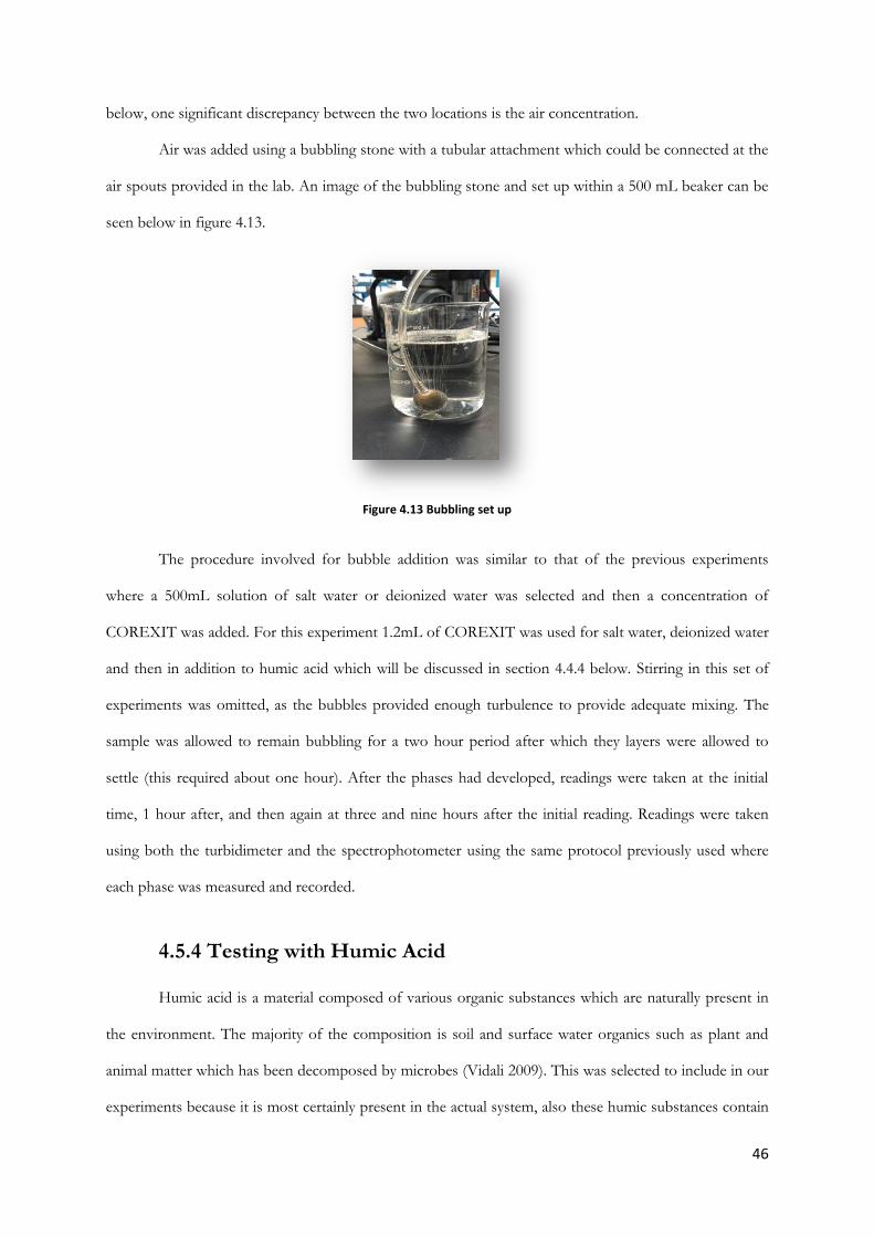
46
below, one significant discrepancy between the two locations is the air concentration.
Air was added using a bubbling stone with a tubular attachment which could be connected at the
air spouts provided in the lab. An image of the bubbling stone and set up within a 500 mL beaker can be
seen below in figure 4.13.
Figure 4.13 Bubbling set up
The procedure involved for bubble addition was similar to that of the previous experiments
where a 500mL solution of salt water or deionized water was selected and then a concentration of
COREXIT was added. For this experiment 1.2mL of COREXIT was used for salt water, deionized water
and then in addition to humic acid which will be discussed in section 4.4.4 below. Stirring in this set of
experiments was omitted, as the bubbles provided enough turbulence to provide adequate mixing. The
sample was allowed to remain bubbling for a two hour period after which they layers were allowed to
settle (this required about one hour). After the phases had developed, readings were taken at the initial
time, 1 hour after, and then again at three and nine hours after the initial reading. Readings were taken
using both the turbidimeter and the spectrophotometer using the same protocol previously used where
each phase was measured and recorded.
4.5.4 Testing with Humic Acid Humic acid is a material composed of various organic substances which are naturally present in
the environment. The majority of the composition is soil and surface water organics such as plant and
animal matter which has been decomposed by microbes (Vidali 2009). This was selected to include in our
experiments because it is most certainly present in the actual system, also these humic substances contain
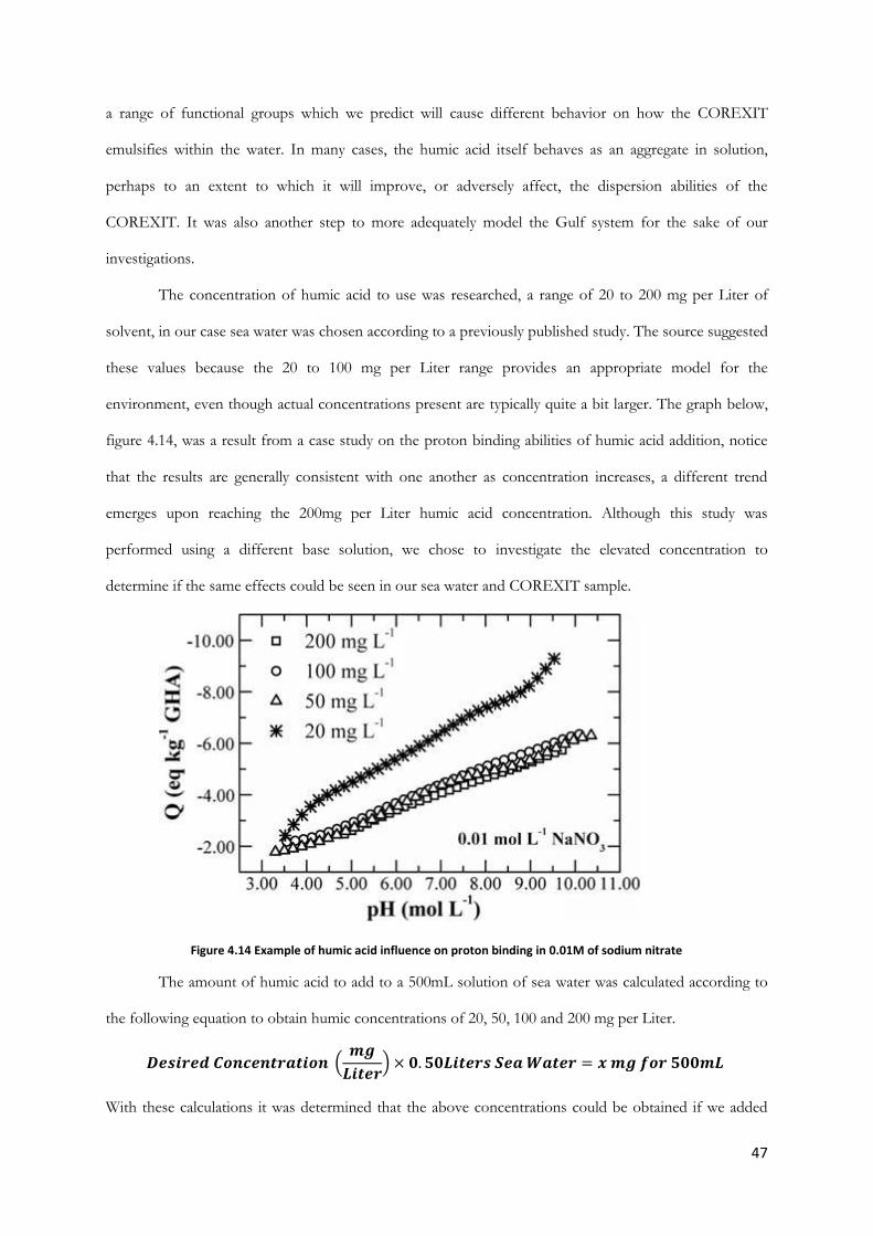
47
a range of functional groups which we predict will cause different behavior on how the COREXIT
emulsifies within the water. In many cases, the humic acid itself behaves as an aggregate in solution,
perhaps to an extent to which it will improve, or adversely affect, the dispersion abilities of the
COREXIT. It was also another step to more adequately model the Gulf system for the sake of our
investigations.
The concentration of humic acid to use was researched, a range of 20 to 200 mg per Liter of
solvent, in our case sea water was chosen according to a previously published study. The source suggested
these values because the 20 to 100 mg per Liter range provides an appropriate model for the
environment, even though actual concentrations present are typically quite a bit larger. The graph below,
figure 4.14, was a result from a case study on the proton binding abilities of humic acid addition, notice
that the results are generally consistent with one another as concentration increases, a different trend
emerges upon reaching the 200mg per Liter humic acid concentration. Although this study was
performed using a different base solution, we chose to investigate the elevated concentration to
determine if the same effects could be seen in our sea water and COREXIT sample.
Figure 4.14 Example of humic acid influence on proton binding in 0.01M of sodium nitrate
The amount of humic acid to add to a 500mL solution of sea water was calculated according to
the following equation to obtain humic concentrations of 20, 50, 100 and 200 mg per Liter.
(
)
With these calculations it was determined that the above concentrations could be obtained if we added
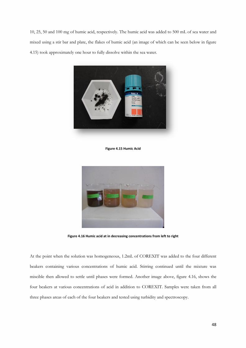
48
10, 25, 50 and 100 mg of humic acid, respectively. The humic acid was added to 500 mL of sea water and
mixed using a stir bar and plate, the flakes of humic acid (an image of which can be seen below in figure
4.15) took approximately one hour to fully dissolve within the sea water.
Figure 4.15 Humic Acid
Figure 4.16 Humic acid at in decreasing concentrations from left to right
At the point when the solution was homogeneous, 1.2mL of COREXIT was added to the four different
beakers containing various concentrations of humic acid. Stirring continued until the mixture was
miscible then allowed to settle until phases were formed. Another image above, figure 4.16, shows the
four beakers at various concentrations of acid in addition to COREXIT. Samples were taken from all
three phases areas of each of the four beakers and tested using turbidity and spectroscopy.
49
4.5.4.1 Humic Acid with Bubble Addition This experiment was performed after observing the results of the bubbles with the standard sea
water and deionized water. The resulting readings were very similar to the initial values but further
investigation was taken to rule out whether or not bubbles indeed did or did not have an effect on the
mixture.
The same solutions formed for the humic acid initial experiment were used for this second set.
Using the same procedure as was used for the system without humic acid, where the bubbles themselves
provided significant mixture, the solution was allowed to bubble for 2 hours after which it rested for
approximately 1 hour until the phases formed. Samples were taken from each level of the solution and
tested using the turbidimeter and spectrophotometer.
4.5.5 Temperature Adjustment
The change in temperature of the body of water that a dispersant is applied to is of vital
importance. To characterize how the change in temperature affects the emulsion formed when
COREXIT 9500A in added to seawater was investigated. In April, in the Gulf of Mexico when the
Deepwater Horizon oil spill took place the temperature was between the ranges of 15°C to 30°C. Since
the conditions in the Gulf of Mexico changes over time examining how COREXIT 9500A changes with
these conditions will be important for future use of this dispersant to inform the user of features that they
may be unaware of.
The experiment created tested how COREXIT 9500A formed an emulsion with the simulated
seawater at three temperatures that was indicative of three of the broadest ranges. A refrigerated
temperature of 10 °C, room temperature at 26 °C and an increased temperature at 36 °C were used as a
template to illustrate the three main changes that are possible in the Gulf of Mexico. The temperatures

50
provide a standard room temperature that increased and decreased from its original temperature so that
the effect of both of those changes could be quantified and analyzed. These temperature ranges were
chosen to give a qualitative outlook on how the change in temperature affects emulsion formation.
Using three temperatures that were easily attainable in the laboratory was of significant
importance. It was important to ensure that multiple experiments could be done at the same temperatures
and there was uniformity between the conditions used. Room temperature was used as the median
between the two other temperatures because it was the easiest to perform because no heating or cooling
source was necessary. Due to the lack of isolated cooling units a preset refrigerator temperature had to be
used for the lower temperature range. Since heating units were easily found in the lab, the temperature of
36 degrees was chosen for several reasons. A 10 degree increase was used for the increased temperature
because increasing the temperature by 10 degrees should double the reaction rate as denoted by reaction
kinetics principles. It was also easy to maintain the heating unit at that elevated temperature for a
prolonged period of time without straining the unit or wasting excessive energy.
The procedure for temperature readings – room temp
Four beakers were labeled A, B C and D. (A) represented refrigerated temperature, (B) denoted
room temperature, (C) represented increased temperature and (D) denoted increased temperature with
increased COREXIT volume. Four portions of 500mL of simulated seawater were added to four 500mL
beakers. A stirrer bar was added to each beaker and then the beakers were placed on stirrers. The stirrers
were turned on to a low setting to create a uniform mixture. A 10mL measuring cylinder was used to
measure 1.5mL of COREXIT 9500A three times and 2.0mL of COREXIT 9500A. The three 1.5mL of
COREXIT was poured gently into the center of the beakers labeled A, B and C while the 2.0mL of
COREXIT was poured gently into the center of the beaker labeled D. The mixture were allowed to mix
for 30 minutes before the stirrer was turned off and covered with paraffin. The time was noted and the
beakers were left to sit at room temperature for 4 hours before spectroscopy readings were done and then
spectroscopy readings were subsequently repeated for kinetic data at the 8, 24 and the 48 hour mark. The
procedure was repeated for the refrigerated and heated temperatures.

51
For the mixtures that were used for the refrigerated temperatures after the stirrer was stopped
the mixtures were transferred to closed cap bottles with the same labels. They were put immediately in
the refrigerator and after 4 hours they were taken out for spectroscopy readings. The readings at the time
intervals mentioned above were also carried out. After the 96 hour spectroscopy readings were done the
bottles were transferred to room temperature and left to settle for 2 days in order to see if the emulsion
formed was affected by a change in temperature. After the mixture was settled spectroscopy readings
were taken and noted. For the heated mixtures instead of being placed in the refrigerator they were placed
in an oven at 36°C but they followed the same procedure as the mixtures in the refrigerator.
1.5mL of COREXIT was used because it was higher than the critical micelle concentration
(CMC) volume of 1.1mL. To ensure that a large, observable emulsion layer was formed 1.5mL of
COREXIT was used as opposed to 1.2mL which would have just been over the estimated value observed
from previous experiments.
4.5.6 Oil Addition
To this point the actual system in the Gulf of Mexico was not being represented accurately
instead the COREXIT 9500A was being characterized for its properties independently from the
COREXIT and oil mixture. The emulsion was being formed in a mixture solely consisting of COREXIT
and simulated seawater. Experimenting how COREXIT emulsion formed with a seawater system only
will help to characterize what should happen if the same condition changes were to occur in an oil and
seawater system. Therefore examining the COREXIT, seawater and oil system provided valuable insight
into what changes could possibly occur with variances in the mixing ratio of the three components.
Two sets of experiments were undertaken; the first involved using a fixed volume of oil and
increasing the volume of COREXIT. On the other hand, the second experiments involved using a fixed
volume of COREXIT and increasing the volume of oil in the system. The first experiment covered the
span of what happens as the COREXIT 9500A is increased in volume and the oil to seawater ratio stays
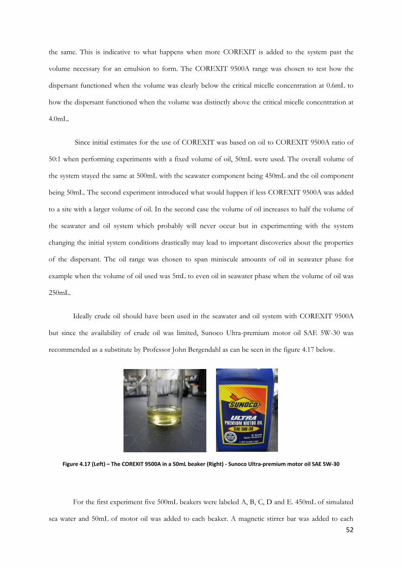
52
the same. This is indicative to what happens when more COREXIT is added to the system past the
volume necessary for an emulsion to form. The COREXIT 9500A range was chosen to test how the
dispersant functioned when the volume was clearly below the critical micelle concentration at 0.6mL to
how the dispersant functioned when the volume was distinctly above the critical micelle concentration at
4.0mL.
Since initial estimates for the use of COREXIT was based on oil to COREXIT 9500A ratio of
50:1 when performing experiments with a fixed volume of oil, 50mL were used. The overall volume of
the system stayed the same at 500mL with the seawater component being 450mL and the oil component
being 50mL. The second experiment introduced what would happen if less COREXIT 9500A was added
to a site with a larger volume of oil. In the second case the volume of oil increases to half the volume of
the seawater and oil system which probably will never occur but in experimenting with the system
changing the initial system conditions drastically may lead to important discoveries about the properties
of the dispersant. The oil range was chosen to span miniscule amounts of oil in seawater phase for
example when the volume of oil used was 5mL to even oil in seawater phase when the volume of oil was
250mL.
Ideally crude oil should have been used in the seawater and oil system with COREXIT 9500A
but since the availability of crude oil was limited, Sunoco Ultra-premium motor oil SAE 5W-30 was
recommended as a substitute by Professor John Bergendahl as can be seen in the figure 4.17 below.
Figure 4.17 (Left) – The COREXIT 9500A in a 50mL beaker (Right) - Sunoco Ultra-premium motor oil SAE 5W-30
For the first experiment five 500mL beakers were labeled A, B, C, D and E. 450mL of simulated
sea water and 50mL of motor oil was added to each beaker. A magnetic stirrer bar was added to each
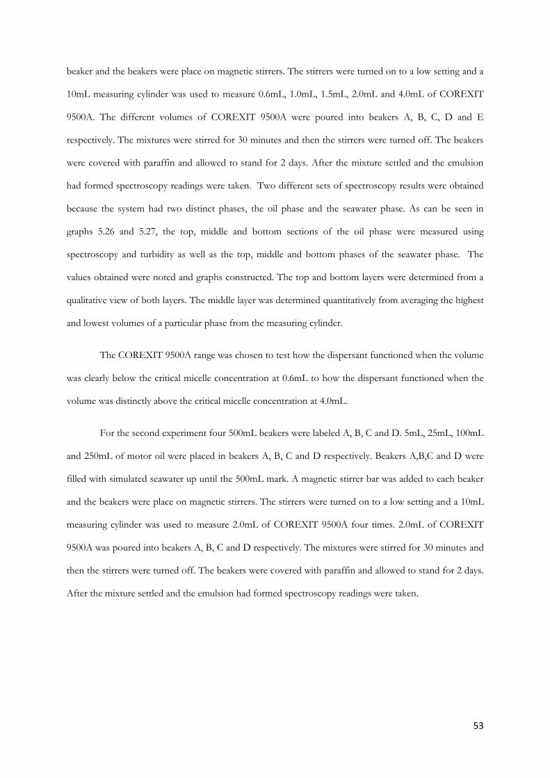
53
beaker and the beakers were place on magnetic stirrers. The stirrers were turned on to a low setting and a
10mL measuring cylinder was used to measure 0.6mL, 1.0mL, 1.5mL, 2.0mL and 4.0mL of COREXIT
9500A. The different volumes of COREXIT 9500A were poured into beakers A, B, C, D and E
respectively. The mixtures were stirred for 30 minutes and then the stirrers were turned off. The beakers
were covered with paraffin and allowed to stand for 2 days. After the mixture settled and the emulsion
had formed spectroscopy readings were taken. Two different sets of spectroscopy results were obtained
because the system had two distinct phases, the oil phase and the seawater phase. As can be seen in
graphs 5.26 and 5.27, the top, middle and bottom sections of the oil phase were measured using
spectroscopy and turbidity as well as the top, middle and bottom phases of the seawater phase. The
values obtained were noted and graphs constructed. The top and bottom layers were determined from a
qualitative view of both layers. The middle layer was determined quantitatively from averaging the highest
and lowest volumes of a particular phase from the measuring cylinder.
The COREXIT 9500A range was chosen to test how the dispersant functioned when the volume
was clearly below the critical micelle concentration at 0.6mL to how the dispersant functioned when the
volume was distinctly above the critical micelle concentration at 4.0mL.
For the second experiment four 500mL beakers were labeled A, B, C and D. 5mL, 25mL, 100mL
and 250mL of motor oil were placed in beakers A, B, C and D respectively. Beakers A,B,C and D were
filled with simulated seawater up until the 500mL mark. A magnetic stirrer bar was added to each beaker
and the beakers were place on magnetic stirrers. The stirrers were turned on to a low setting and a 10mL
measuring cylinder was used to measure 2.0mL of COREXIT 9500A four times. 2.0mL of COREXIT
9500A was poured into beakers A, B, C and D respectively. The mixtures were stirred for 30 minutes and
then the stirrers were turned off. The beakers were covered with paraffin and allowed to stand for 2 days.
After the mixture settled and the emulsion had formed spectroscopy readings were taken.
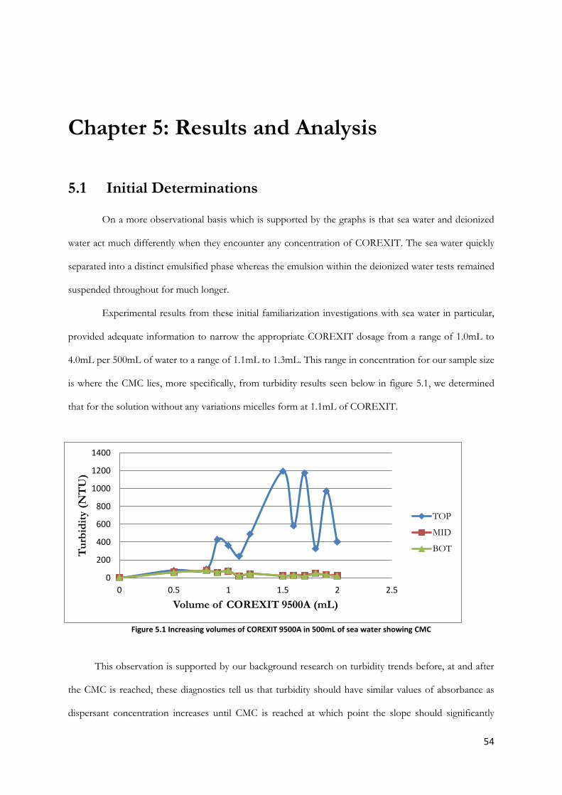
54
0
200
400
600
800
1000
1200
1400
0 0.5 1 1.5 2 2.5
Tu
rbid
ity (
NT
U)
Volume of COREXIT 9500A (mL)
TOP
MID
BOT
Chapter 5: Results and Analysis
5.1 Initial Determinations
On a more observational basis which is supported by the graphs is that sea water and deionized
water act much differently when they encounter any concentration of COREXIT. The sea water quickly
separated into a distinct emulsified phase whereas the emulsion within the deionized water tests remained
suspended throughout for much longer.
Experimental results from these initial familiarization investigations with sea water in particular,
provided adequate information to narrow the appropriate COREXIT dosage from a range of 1.0mL to
4.0mL per 500mL of water to a range of 1.1mL to 1.3mL. This range in concentration for our sample size
is where the CMC lies, more specifically, from turbidity results seen below in figure 5.1, we determined
that for the solution without any variations micelles form at 1.1mL of COREXIT.
Figure 5.1 Increasing volumes of COREXIT 9500A in 500mL of sea water showing CMC
This observation is supported by our background research on turbidity trends before, at and after
the CMC is reached, these diagnostics tell us that turbidity should have similar values of absorbance as
dispersant concentration increases until CMC is reached at which point the slope should significantly
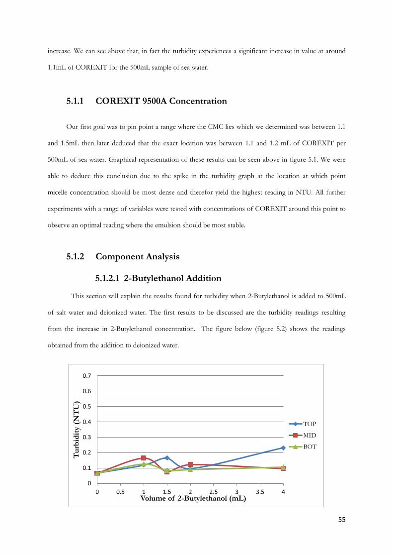
55
increase. We can see above that, in fact the turbidity experiences a significant increase in value at around
1.1mL of COREXIT for the 500mL sample of sea water.
5.1.1 COREXIT 9500A Concentration
Our first goal was to pin point a range where the CMC lies which we determined was between 1.1
and 1.5mL then later deduced that the exact location was between 1.1 and 1.2 mL of COREXIT per
500mL of sea water. Graphical representation of these results can be seen above in figure 5.1. We were
able to deduce this conclusion due to the spike in the turbidity graph at the location at which point
micelle concentration should be most dense and therefor yield the highest reading in NTU. All further
experiments with a range of variables were tested with concentrations of COREXIT around this point to
observe an optimal reading where the emulsion should be most stable.
5.1.2 Component Analysis
5.1.2.1 2-Butylethanol Addition
This section will explain the results found for turbidity when 2-Butylethanol is added to 500mL
of salt water and deionized water. The first results to be discussed are the turbidity readings resulting
from the increase in 2-Butylethanol concentration. The figure below (figure 5.2) shows the readings
obtained from the addition to deionized water.
0
0.1
0.2
0.3
0.4
0.5
0.6
0.7
0 0.5 1 1.5 2 2.5 3 3.5 4
Tu
rbid
ity (
NT
U)
Volume of 2-Butylethanol (mL)
TOP
MID
BOT
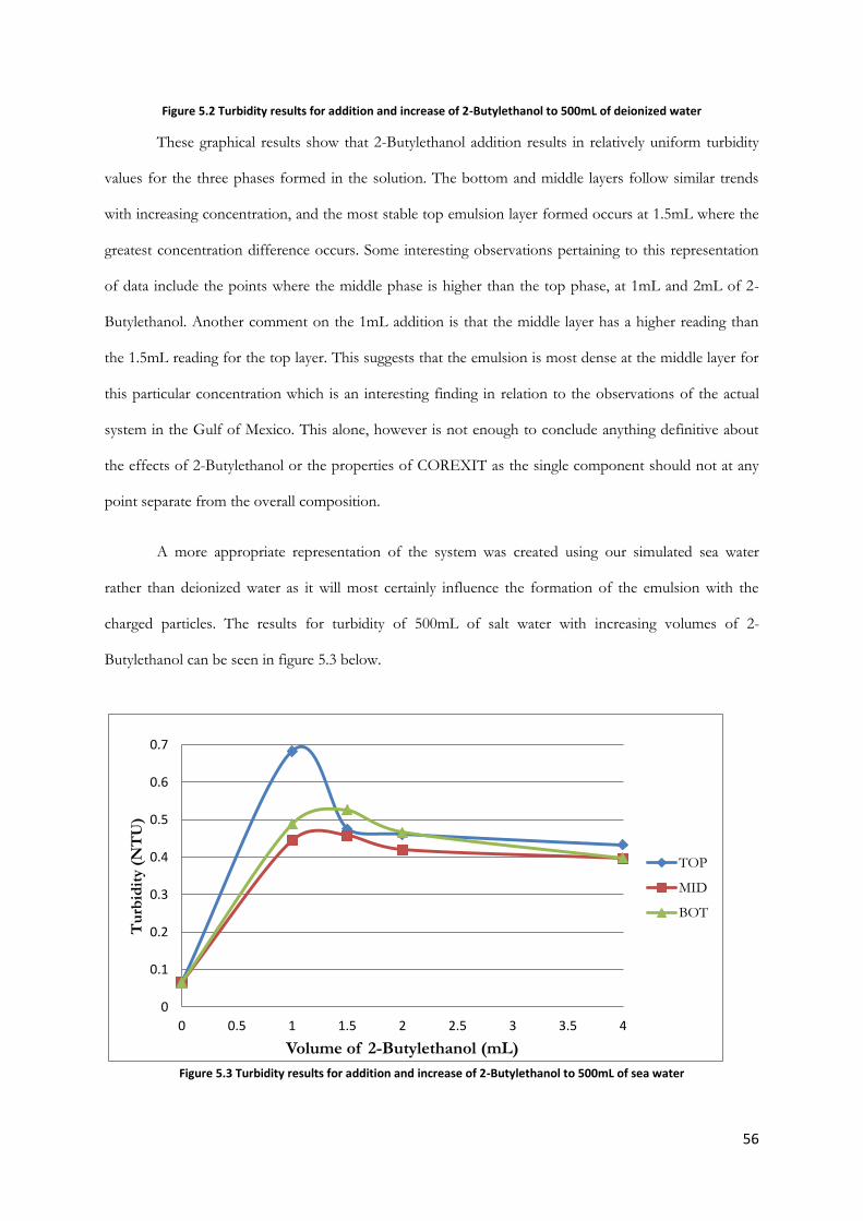
56
Figure 5.2 Turbidity results for addition and increase of 2-Butylethanol to 500mL of deionized water
These graphical results show that 2-Butylethanol addition results in relatively uniform turbidity
values for the three phases formed in the solution. The bottom and middle layers follow similar trends
with increasing concentration, and the most stable top emulsion layer formed occurs at 1.5mL where the
greatest concentration difference occurs. Some interesting observations pertaining to this representation
of data include the points where the middle phase is higher than the top phase, at 1mL and 2mL of 2-
Butylethanol. Another comment on the 1mL addition is that the middle layer has a higher reading than
the 1.5mL reading for the top layer. This suggests that the emulsion is most dense at the middle layer for
this particular concentration which is an interesting finding in relation to the observations of the actual
system in the Gulf of Mexico. This alone, however is not enough to conclude anything definitive about
the effects of 2-Butylethanol or the properties of COREXIT as the single component should not at any
point separate from the overall composition.
A more appropriate representation of the system was created using our simulated sea water
rather than deionized water as it will most certainly influence the formation of the emulsion with the
charged particles. The results for turbidity of 500mL of salt water with increasing volumes of 2-
Butylethanol can be seen in figure 5.3 below.
Figure 5.3 Turbidity results for addition and increase of 2-Butylethanol to 500mL of sea water
0
0.1
0.2
0.3
0.4
0.5
0.6
0.7
0 0.5 1 1.5 2 2.5 3 3.5 4
Tu
rbid
ity (
NT
U)
Volume of 2-Butylethanol (mL)
TOP
MID
BOT

57
The results from the plotted turbidity measurements display a consistent shape trend in turbidity as
the volume of 2-Butylethanol increases. All three phases display a large slope from the basis reading
where no 2-Butylethanol was added, to the 1mL addition of the top layer and 1.5mL addition for the
middle and bottom samples. For increasing concentrations past this point the turbidity measurements
decrease gradually and level after 2mL of 2-Butylethanol.
A significant deviation from the predictions on the phase formation behavior is that the bottom
phase has consistently higher readings than the middle layer; this suggests that there is a larger emulsion
concentration on the lowest sampling point within the system. The greatest difference between the top
reading and the middle and bottom layers occurs at around 1.1mL of 2-Butylethanol which agrees with
the determination that the CMC lies at relatively the same volume of COREXIT.
A major comparison between the use of deionized water and sea water is that the readings of the
latter are much larger in comparison. Similarly, the range in values for the sea water is greater than the
deionized water with values ranging within 0.1 NTU of each other. More distinct phase formations occur
in the salt water experiments, meaning more stable emulsion formation.
5.1.2.2 Sodium bis(2-ethylhexyl) Sulfosuccinate Addition
The proceeding section will present and discuss the results found for the addition of sodium
bis(2-ethylhexyl)sulfosuccinate to deionized and sea water solutions. Turbidity and spectroscopy
collections were executed for this component addition. First turbidity results will be discussed and
compared followed by an evaluation of the spectroscopy experiments. Figures 5.4 through 5.7 below
graphically display the experimental findings, beginning with sodium bis(2-ethylhexyl)sulfosuccinate
addition to deionized water.
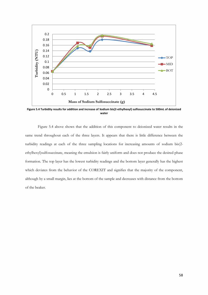
58
Figure 5.4 Turbidity results for addition and increase of sodium bis(2-ethylhexyl) sulfosuccinate to 500mL of deionized
water
Figure 5.4 above shows that the addition of this component to deionized water results in the
same trend throughout each of the three layers. It appears that there is little difference between the
turbidity readings at each of the three sampling locations for increasing amounts of sodium bis(2-
ethylhexyl)sulfosuccinate, meaning the emulsion is fairly uniform and does not produce the desired phase
formation. The top layer has the lowest turbidity readings and the bottom layer generally has the highest
which deviates from the behavior of the COREXIT and signifies that the majority of the component,
although by a small margin, lies at the bottom of the sample and decreases with distance from the bottom
of the beaker.
0
0.02
0.04
0.06
0.08
0.1
0.12
0.14
0.16
0.18
0.2
0 0.5 1 1.5 2 2.5 3 3.5 4 4.5
Tu
rbid
ity (
NT
U)
Mass of Sodium Sulfosuccinate (g)
TOP
MID
BOT
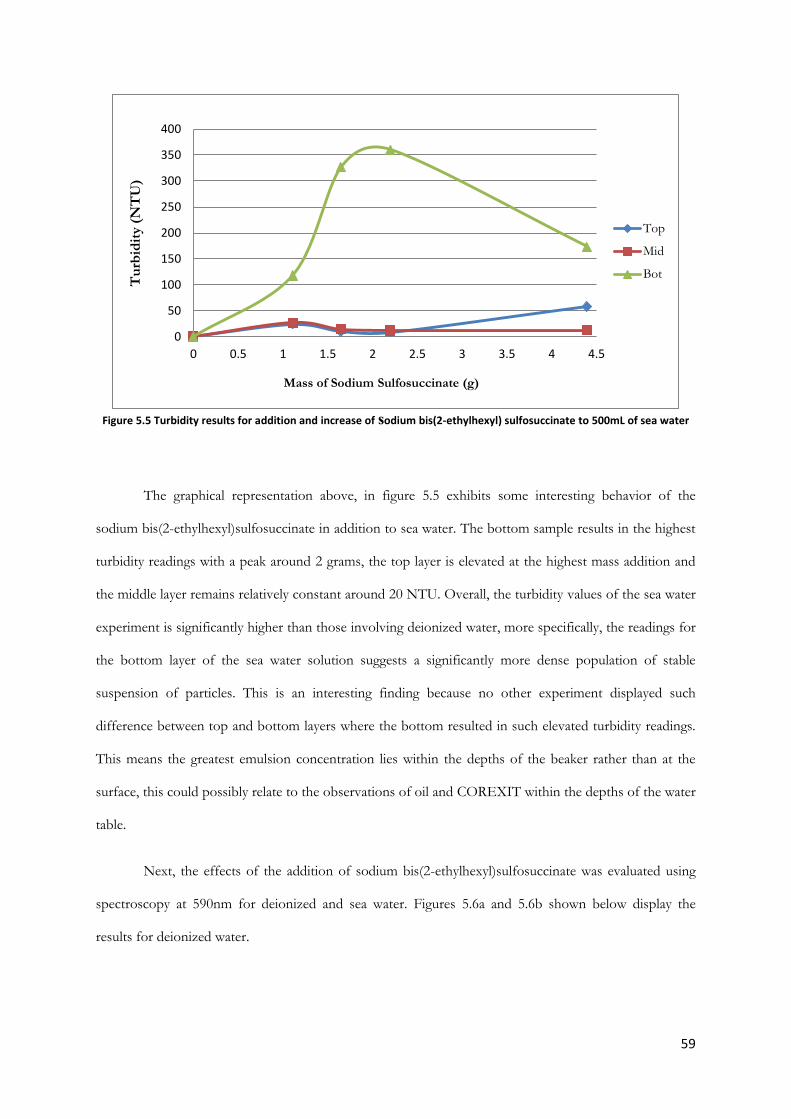
59
Figure 5.5 Turbidity results for addition and increase of sodium bis(2-ethylhexyl) sulfosuccinate to 500mL of sea water
The graphical representation above, in figure 5.5 exhibits some interesting behavior of the
sodium bis(2-ethylhexyl)sulfosuccinate in addition to sea water. The bottom sample results in the highest
turbidity readings with a peak around 2 grams, the top layer is elevated at the highest mass addition and
the middle layer remains relatively constant around 20 NTU. Overall, the turbidity values of the sea water
experiment is significantly higher than those involving deionized water, more specifically, the readings for
the bottom layer of the sea water solution suggests a significantly more dense population of stable
suspension of particles. This is an interesting finding because no other experiment displayed such
difference between top and bottom layers where the bottom resulted in such elevated turbidity readings.
This means the greatest emulsion concentration lies within the depths of the beaker rather than at the
surface, this could possibly relate to the observations of oil and COREXIT within the depths of the water
table.
Next, the effects of the addition of sodium bis(2-ethylhexyl)sulfosuccinate was evaluated using
spectroscopy at 590nm for deionized and sea water. Figures 5.6a and 5.6b shown below display the
results for deionized water.
0
50
100
150
200
250
300
350
400
0 0.5 1 1.5 2 2.5 3 3.5 4 4.5
Tu
rbid
ity (
NT
U)
Mass of Sodium Sulfosuccinate (g)
Top
Mid
Bot
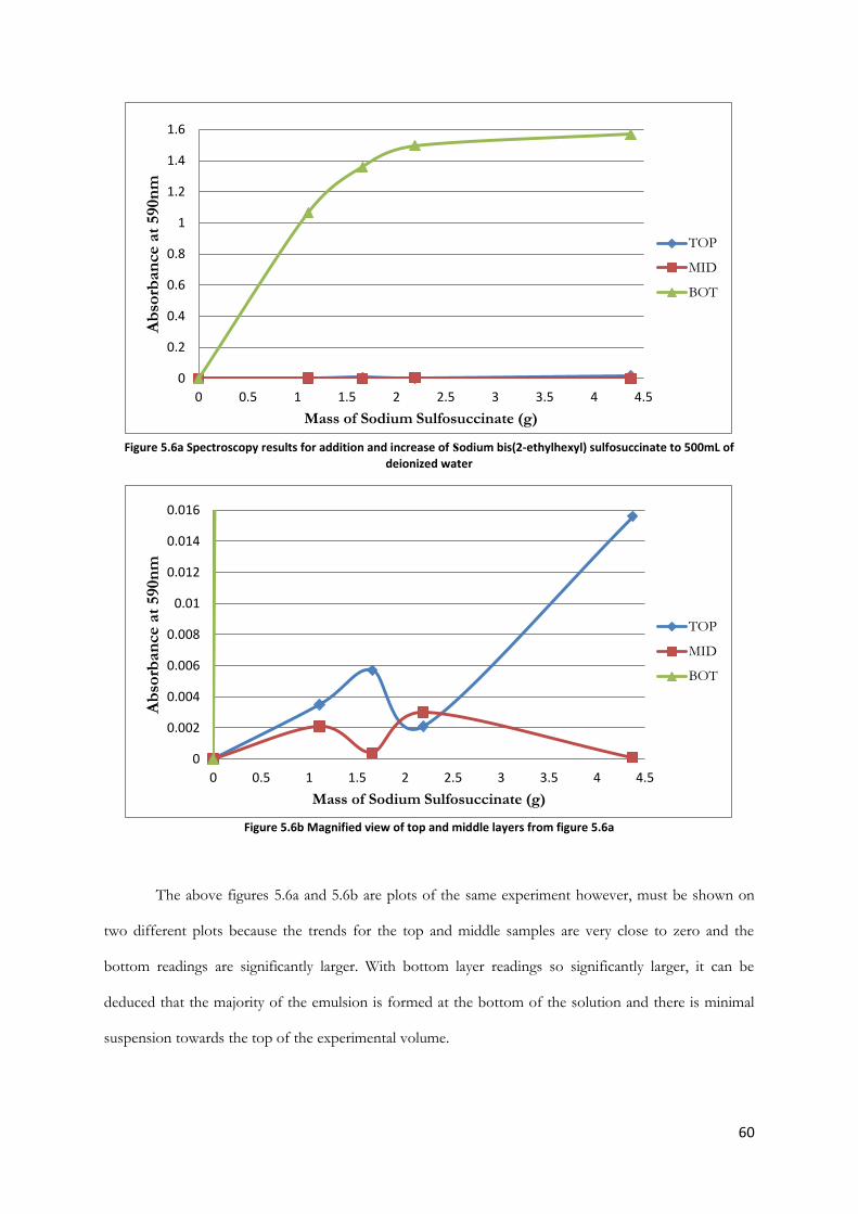
60
Figure 5.6a Spectroscopy results for addition and increase of sodium bis(2-ethylhexyl) sulfosuccinate to 500mL of
deionized water
Figure 5.6b Magnified view of top and middle layers from figure 5.6a
The above figures 5.6a and 5.6b are plots of the same experiment however, must be shown on
two different plots because the trends for the top and middle samples are very close to zero and the
bottom readings are significantly larger. With bottom layer readings so significantly larger, it can be
deduced that the majority of the emulsion is formed at the bottom of the solution and there is minimal
suspension towards the top of the experimental volume.
0
0.2
0.4
0.6
0.8
1
1.2
1.4
1.6
0 0.5 1 1.5 2 2.5 3 3.5 4 4.5
Ab
sorb
an
ce a
t 590n
m
Mass of Sodium Sulfosuccinate (g)
TOP
MID
BOT
0
0.002
0.004
0.006
0.008
0.01
0.012
0.014
0.016
0 0.5 1 1.5 2 2.5 3 3.5 4 4.5
Ab
sorb
an
ce a
t 590n
m
Mass of Sodium Sulfosuccinate (g)
TOP
MID
BOT
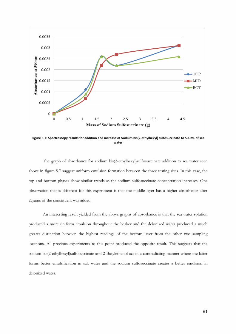
61
Figure 5.7: Spectroscopy results for addition and increase of sodium bis(2-ethylhexyl) sulfosuccinate to 500mL of sea
water
The graph of absorbance for sodium bis(2-ethylhexyl)sulfosuccinate addition to sea water seen
above in figure 5.7 suggest uniform emulsion formation between the three testing sites. In this case, the
top and bottom phases show similar trends as the sodium sulfosuccinate concentration increases. One
observation that is different for this experiment is that the middle layer has a higher absorbance after
2grams of the constituent was added.
An interesting result yielded from the above graphs of absorbance is that the sea water solution
produced a more uniform emulsion throughout the beaker and the deionized water produced a much
greater distinction between the highest readings of the bottom layer from the other two sampling
locations. All previous experiments to this point produced the opposite result. This suggests that the
sodium bis(2-ethylhexyl)sulfosuccinate and 2-Butylethanol act in a contradicting manner where the latter
forms better emulsification in salt water and the sodium sulfosuccinate creates a better emulsion in
deionized water.
0
0.0005
0.001
0.0015
0.002
0.0025
0.003
0.0035
0 0.5 1 1.5 2 2.5 3 3.5 4 4.5
Ab
sorb
an
ce a
t 590n
m
Mass of Sodium Sulfosuccinate (g)
TOP
MID
BOT
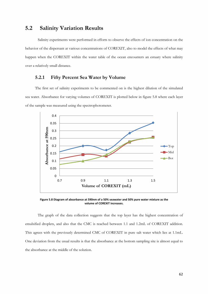
62
5.2 Salinity Variation Results
Salinity experiments were performed in efforts to observe the effects of ion concentration on the
behavior of the dispersant at various concentrations of COREXIT, also to model the effects of what may
happen when the COREXIT within the water table of the ocean encounters an estuary where salinity
over a relatively small distance.
5.2.1 Fifty Percent Sea Water by Volume The first set of salinity experiments to be commented on is the highest dilution of the simulated
sea water. Absorbance for varying volumes of COREXIT is plotted below in figure 5.8 where each layer
of the sample was measured using the spectrophotometer.
Figure 5.8 Diagram of absorbance at 590nm of a 50% seawater and 50% pure water mixture as the volume of COREXIT increases.
The graph of the data collection suggests that the top layer has the highest concentration of
emulsified droplets, and also that the CMC is reached between 1.1 and 1.2mL of COREXIT addition.
This agrees with the previously determined CMC of COREXIT in pure salt water which lies at 1.1mL.
One deviation from the usual results is that the absorbance at the bottom sampling site is almost equal to
the absorbance at the middle of the solution.
0
0.05
0.1
0.15
0.2
0.25
0.3
0.35
0.4
0.7 0.9 1.1 1.3 1.5
Ab
sorb
an
ce a
t 590n
m
Volume of COREXIT (mL)
Top
Mid
Bot
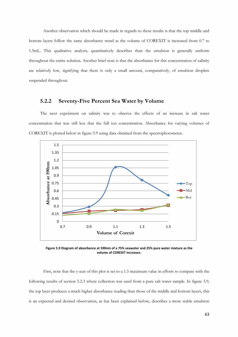
63
Another observation which should be made in regards to these results is that the top middle and
bottom layers follow the same absorbance trend as the volume of COREXIT is increased from 0.7 to
1.5mL. This qualitative analysis, quantitatively describes than the emulsion is generally uniform
throughout the entire solution. Another brief note is that the absorbance for this concentration of salinity
are relatively low, signifying that there is only a small amount, comparatively, of emulsion droplets
suspended throughout.
5.2.2 Seventy-Five Percent Sea Water by Volume
The next experiment on salinity was to observe the effects of an increase in salt water
concentration that was still less that the full ion concentration. Absorbance for varying volumes of
COREXIT is plotted below in figure 5.9 using data obtained from the spectrophotometer.
Figure 5.9 Diagram of absorbance at 590nm of a 75% seawater and 25% pure water mixture as the volume of COREXIT increases.
First, note that the y-axis of this plot is set to a 1.5 maximum value in efforts to compare with the
following results of section 5.2.3 where collection was used from a pure salt water sample. In figure 5.9,
the top layer produces a much higher absorbance reading than those of the middle and bottom layers, this
is an expected and desired observation, as has been explained before, describes a more stable emulsion
0
0.15
0.3
0.45
0.6
0.75
0.9
1.05
1.2
1.35
1.5
0.7 0.9 1.1 1.3 1.5
Ab
sorb
an
ce a
t 590n
m
Volume of Corexit
Top
Mid
Bot
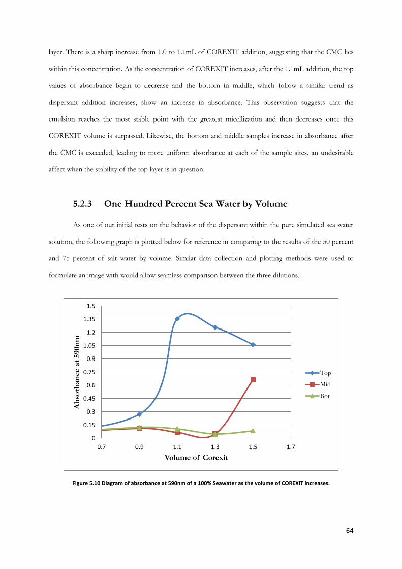
64
layer. There is a sharp increase from 1.0 to 1.1mL of COREXIT addition, suggesting that the CMC lies
within this concentration. As the concentration of COREXIT increases, after the 1.1mL addition, the top
values of absorbance begin to decrease and the bottom in middle, which follow a similar trend as
dispersant addition increases, show an increase in absorbance. This observation suggests that the
emulsion reaches the most stable point with the greatest micellization and then decreases once this
COREXIT volume is surpassed. Likewise, the bottom and middle samples increase in absorbance after
the CMC is exceeded, leading to more uniform absorbance at each of the sample sites, an undesirable
affect when the stability of the top layer is in question.
5.2.3 One Hundred Percent Sea Water by Volume As one of our initial tests on the behavior of the dispersant within the pure simulated sea water
solution, the following graph is plotted below for reference in comparing to the results of the 50 percent
and 75 percent of salt water by volume. Similar data collection and plotting methods were used to
formulate an image with would allow seamless comparison between the three dilutions.
Figure 5.10 Diagram of absorbance at 590nm of a 100% Seawater as the volume of COREXIT increases.
0
0.15
0.3
0.45
0.6
0.75
0.9
1.05
1.2
1.35
1.5
0.7 0.9 1.1 1.3 1.5 1.7
Ab
sorb
an
ce a
t 590n
m
Volume of Corexit
Top
Mid
Bot
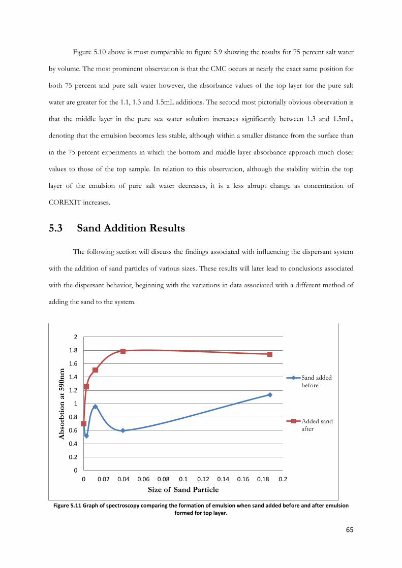
65
Figure 5.10 above is most comparable to figure 5.9 showing the results for 75 percent salt water
by volume. The most prominent observation is that the CMC occurs at nearly the exact same position for
both 75 percent and pure salt water however, the absorbance values of the top layer for the pure salt
water are greater for the 1.1, 1.3 and 1.5mL additions. The second most pictorially obvious observation is
that the middle layer in the pure sea water solution increases significantly between 1.3 and 1.5mL,
denoting that the emulsion becomes less stable, although within a smaller distance from the surface than
in the 75 percent experiments in which the bottom and middle layer absorbance approach much closer
values to those of the top sample. In relation to this observation, although the stability within the top
layer of the emulsion of pure salt water decreases, it is a less abrupt change as concentration of
COREXIT increases.
5.3 Sand Addition Results The following section will discuss the findings associated with influencing the dispersant system
with the addition of sand particles of various sizes. These results will later lead to conclusions associated
with the dispersant behavior, beginning with the variations in data associated with a different method of
adding the sand to the system.
Figure 5.11 Graph of spectroscopy comparing the formation of emulsion when sand added before and after emulsion
formed for top layer.
0
0.2
0.4
0.6
0.8
1
1.2
1.4
1.6
1.8
2
0 0.02 0.04 0.06 0.08 0.1 0.12 0.14 0.16 0.18 0.2
Ab
sorb
tio
n a
t 590n
m
Size of Sand Particle
Sand addedbefore
Added sandafter
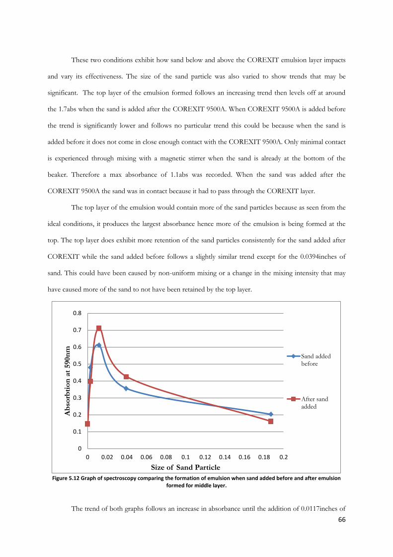
66
These two conditions exhibit how sand below and above the COREXIT emulsion layer impacts
and vary its effectiveness. The size of the sand particle was also varied to show trends that may be
significant. The top layer of the emulsion formed follows an increasing trend then levels off at around
the 1.7abs when the sand is added after the COREXIT 9500A. When COREXIT 9500A is added before
the trend is significantly lower and follows no particular trend this could be because when the sand is
added before it does not come in close enough contact with the COREXIT 9500A. Only minimal contact
is experienced through mixing with a magnetic stirrer when the sand is already at the bottom of the
beaker. Therefore a max absorbance of 1.1abs was recorded. When the sand was added after the
COREXIT 9500A the sand was in contact because it had to pass through the COREXIT layer.
The top layer of the emulsion would contain more of the sand particles because as seen from the
ideal conditions, it produces the largest absorbance hence more of the emulsion is being formed at the
top. The top layer does exhibit more retention of the sand particles consistently for the sand added after
COREXIT while the sand added before follows a slightly similar trend except for the 0.0394inches of
sand. This could have been caused by non-uniform mixing or a change in the mixing intensity that may
have caused more of the sand to not have been retained by the top layer.
Figure 5.12 Graph of spectroscopy comparing the formation of emulsion when sand added before and after emulsion
formed for middle layer.
The trend of both graphs follows an increase in absorbance until the addition of 0.0117inches of
0
0.1
0.2
0.3
0.4
0.5
0.6
0.7
0.8
0 0.02 0.04 0.06 0.08 0.1 0.12 0.14 0.16 0.18 0.2
Ab
sorb
tio
n a
t 590n
m
Size of Sand Particle
Sand addedbefore
After sandadded
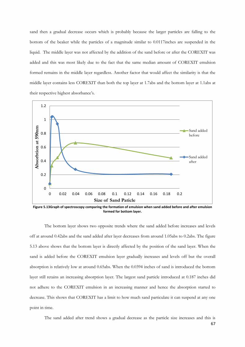
67
sand then a gradual decrease occurs which is probably because the larger particles are falling to the
bottom of the beaker while the particles of a magnitude similar to 0.0117inches are suspended in the
liquid. The middle layer was not affected by the addition of the sand before or after the COREXIT was
added and this was most likely due to the fact that the same median amount of COREXIT emulsion
formed remains in the middle layer regardless. Another factor that would affect the similarity is that the
middle layer contains less COREXIT than both the top layer at 1.7abs and the bottom layer at 1.1abs at
their respective highest absorbance’s.
Figure 5.13Graph of spectroscopy comparing the formation of emulsion when sand added before and after emulsion
formed for bottom layer.
The bottom layer shows two opposite trends where the sand added before increases and levels
off at around 0.42abs and the sand added after layer decreases from around 1.05abs to 0.2abs. The figure
5.13 above shows that the bottom layer is directly affected by the position of the sand layer. When the
sand is added before the COREXIT emulsion layer gradually increases and levels off but the overall
absorption is relatively low at around 0.65abs. When the 0.0394 inches of sand is introduced the bottom
layer still retains an increasing absorption layer. The largest sand particle introduced at 0.187 inches did
not adhere to the COREXIT emulsion in an increasing manner and hence the absorption started to
decrease. This shows that COREXIT has a limit to how much sand particulate it can suspend at any one
point in time.
The sand added after trend shows a gradual decrease as the particle size increases and this is
0
0.2
0.4
0.6
0.8
1
1.2
0 0.02 0.04 0.06 0.08 0.1 0.12 0.14 0.16 0.18 0.2
Ab
sorb
tio
n a
t 590n
m
Size of Sand Paticle
Sand addedbefore
Sand addedafter
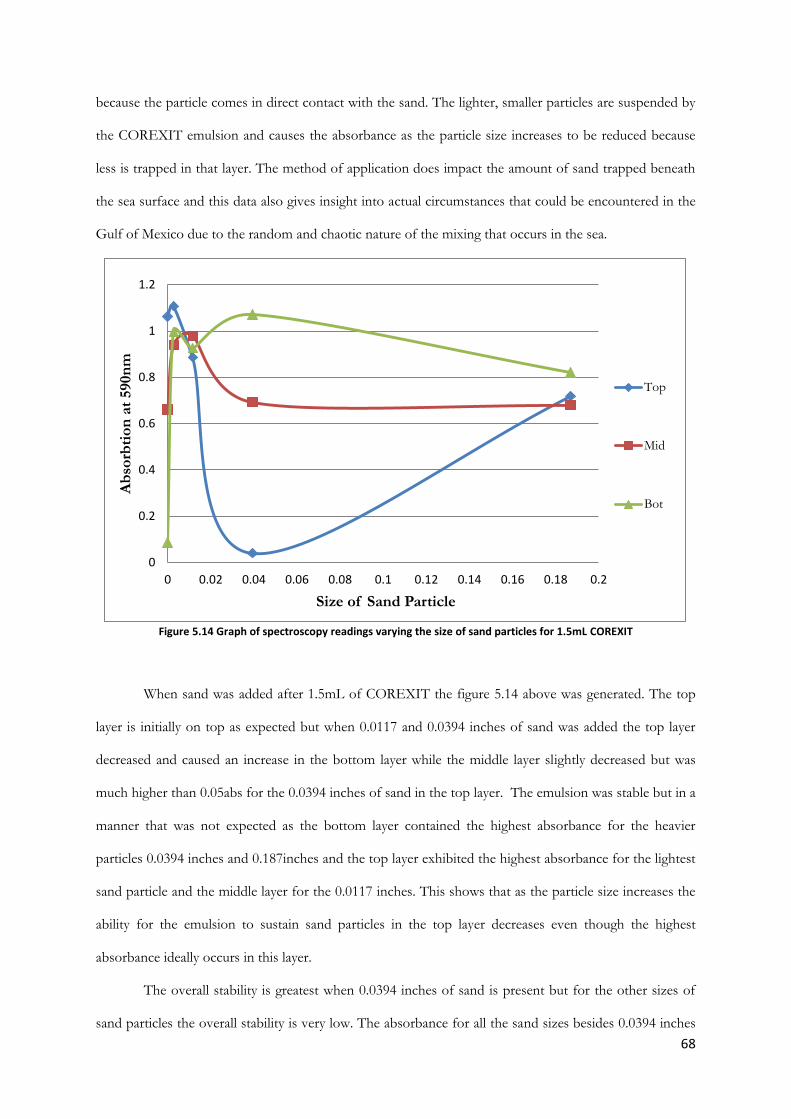
68
because the particle comes in direct contact with the sand. The lighter, smaller particles are suspended by
the COREXIT emulsion and causes the absorbance as the particle size increases to be reduced because
less is trapped in that layer. The method of application does impact the amount of sand trapped beneath
the sea surface and this data also gives insight into actual circumstances that could be encountered in the
Gulf of Mexico due to the random and chaotic nature of the mixing that occurs in the sea.
Figure 5.14 Graph of spectroscopy readings varying the size of sand particles for 1.5mL COREXIT
When sand was added after 1.5mL of COREXIT the figure 5.14 above was generated. The top
layer is initially on top as expected but when 0.0117 and 0.0394 inches of sand was added the top layer
decreased and caused an increase in the bottom layer while the middle layer slightly decreased but was
much higher than 0.05abs for the 0.0394 inches of sand in the top layer. The emulsion was stable but in a
manner that was not expected as the bottom layer contained the highest absorbance for the heavier
particles 0.0394 inches and 0.187inches and the top layer exhibited the highest absorbance for the lightest
sand particle and the middle layer for the 0.0117 inches. This shows that as the particle size increases the
ability for the emulsion to sustain sand particles in the top layer decreases even though the highest
absorbance ideally occurs in this layer.
The overall stability is greatest when 0.0394 inches of sand is present but for the other sizes of
sand particles the overall stability is very low. The absorbance for all the sand sizes besides 0.0394 inches
0
0.2
0.4
0.6
0.8
1
1.2
0 0.02 0.04 0.06 0.08 0.1 0.12 0.14 0.16 0.18 0.2
Ab
sorb
tio
n a
t 590n
m
Size of Sand Particle
Top
Mid
Bot
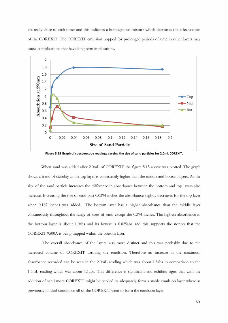
69
are really close to each other and this indicates a homogenous mixture which decreases the effectiveness
of the COREXIT. The COREXIT emulsion trapped for prolonged periods of time in other layers may
cause complications that have long term implications.
Figure 5.15 Graph of spectroscopy readings varying the size of sand particles for 2.0mL COREXIT.
When sand was added after 2.0mL of COREXIT the figure 5.15 above was plotted. The graph
shows a trend of stability as the top layer is consistently higher than the middle and bottom layers. As the
size of the sand particle increases the difference in absorbance between the bottom and top layers also
increase. Increasing the size of sand past 0.0394 inches the absorbance slightly decreases for the top layer
when 0.187 inches was added. The bottom layer has a higher absorbance than the middle layer
continuously throughout the range of sizes of sand except the 0.394 inches. The highest absorbance in
the bottom layer is about 1.0abs and its lowest is 0.025abs and this supports the notion that the
COREXIT 9500A is being trapped within the bottom layer.
The overall absorbance of the layers was more distinct and this was probably due to the
increased volume of COREXIT forming the emulsion. Therefore an increase in the maximum
absorbance recorded can be seen in the 2.0mL reading which was about 1.8abs in comparison to the
1.5mL reading which was about 1.1abs. This difference is significant and exhibits signs that with the
addition of sand more COREXIT might be needed to adequately form a stable emulsion layer where as
previously in ideal conditions all of the COREXIT went to form the emulsion layer.
0
0.2
0.4
0.6
0.8
1
1.2
1.4
1.6
1.8
2
0 0.02 0.04 0.06 0.08 0.1 0.12 0.14 0.16 0.18 0.2
Ab
sorb
tio
n a
t 590n
m
Size of Sand Particle
Top
Mid
Bot
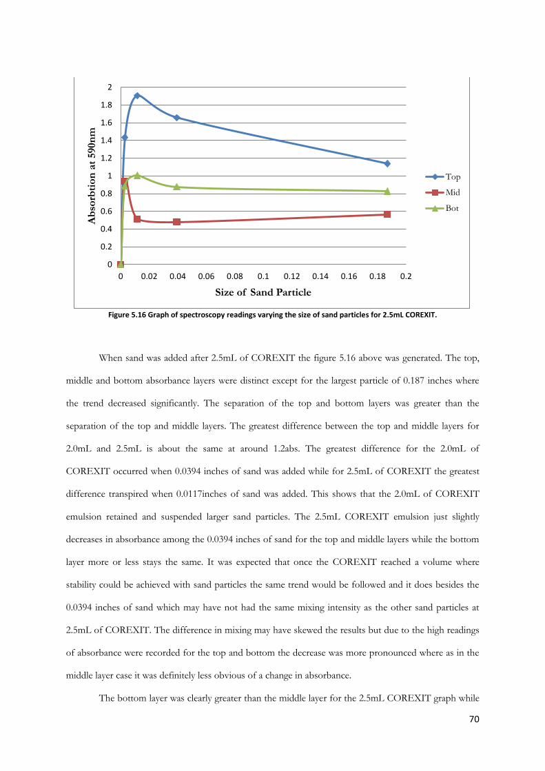
70
Figure 5.16 Graph of spectroscopy readings varying the size of sand particles for 2.5mL COREXIT.
When sand was added after 2.5mL of COREXIT the figure 5.16 above was generated. The top,
middle and bottom absorbance layers were distinct except for the largest particle of 0.187 inches where
the trend decreased significantly. The separation of the top and bottom layers was greater than the
separation of the top and middle layers. The greatest difference between the top and middle layers for
2.0mL and 2.5mL is about the same at around 1.2abs. The greatest difference for the 2.0mL of
COREXIT occurred when 0.0394 inches of sand was added while for 2.5mL of COREXIT the greatest
difference transpired when 0.0117inches of sand was added. This shows that the 2.0mL of COREXIT
emulsion retained and suspended larger sand particles. The 2.5mL COREXIT emulsion just slightly
decreases in absorbance among the 0.0394 inches of sand for the top and middle layers while the bottom
layer more or less stays the same. It was expected that once the COREXIT reached a volume where
stability could be achieved with sand particles the same trend would be followed and it does besides the
0.0394 inches of sand which may have not had the same mixing intensity as the other sand particles at
2.5mL of COREXIT. The difference in mixing may have skewed the results but due to the high readings
of absorbance were recorded for the top and bottom the decrease was more pronounced where as in the
middle layer case it was definitely less obvious of a change in absorbance.
The bottom layer was clearly greater than the middle layer for the 2.5mL COREXIT graph while
0
0.2
0.4
0.6
0.8
1
1.2
1.4
1.6
1.8
2
0 0.02 0.04 0.06 0.08 0.1 0.12 0.14 0.16 0.18 0.2
Ab
sorb
tio
n a
t 590n
m
Size of Sand Particle
Top
Mid
Bot
71
the 2.0mL bottom layer was less distinct. This shows that as the COREXIT is being increasingly trapped
when the volume of COREXIT increases. The absorbance of the 2.5mL of COREXIT is very similar to
the 1.5mL of COREXIT readings at around 1.0abs. However, since the bottom, middle and top layers
were inverted for the two larger sizes of sand for the 1.5mL COREXIT readings the emulsion may not
have been stable but when 2.0mL of COREXIT was added the stability of the predicted layers were
formed. Hence from this initial stability the increase in COREXIT volume to 2.5mL is representative of
an addition to the stable layer which causes more COREXIT to be trapped underneath the middle layer.
For the top layer of both the 2.0mL and 2.5mL volume of COREXIT graphs absorbance decreased when
the larger 0.187 inch sand was added.
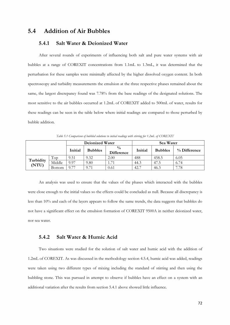
72
5.4 Addition of Air Bubbles
5.4.1 Salt Water & Deionized Water After several rounds of experiments of influencing both salt and pure water systems with air
bubbles at a range of COREXIT concentrations from 1.1mL to 1.3mL, it was determined that the
perturbation for these samples were minimally affected by the higher dissolved oxygen content. In both
spectroscopy and turbidity measurements the emulsion at the three respective phases remained about the
same, the largest discrepancy found was 7.78% from the base readings of the designated solutions. The
most sensitive to the air bubbles occurred at 1.2mL of COREXIT added to 500mL of water, results for
these readings can be seen in the table below where initial readings are compared to those perturbed by
bubble addition.
Table 5.1 Comparison of bubbled solutions to initial readings with stirring for 1.2mL of COREXIT
Deionized Water Sea Water
Initial Bubbles %
Difference Initial Bubbles % Difference
Turbidity (NTU)
Top 9.51 9.32 2.00 488 458.5 6.05
Middle 9.97 9.80 1.71 44.3 47.5 6.74
Bottom 9.77 9.71 0.61 42.7 46.3 7.78
An analysis was used to ensure that the values of the phases which interacted with the bubbles
were close enough to the initial values so the effects could be concluded as null. Because all discrepancy is
less than 10% and each of the layers appears to follow the same trends, the data suggests that bubbles do
not have a significant effect on the emulsion formation of COREXIT 9500A in neither deionized water,
nor sea water.
5.4.2 Salt Water & Humic Acid Two situations were studied for the solution of salt water and humic acid with the addition of
1.2mL of COREXIT. As was discussed in the methodology section 4.5.4, humic acid was added, readings
were taken using two different types of mixing including the standard of stirring and then using the
bubbling stone. This was pursued in attempt to observe if bubbles have an effect on a system with an
additional variation after the results from section 5.4.1 above showed little influence.
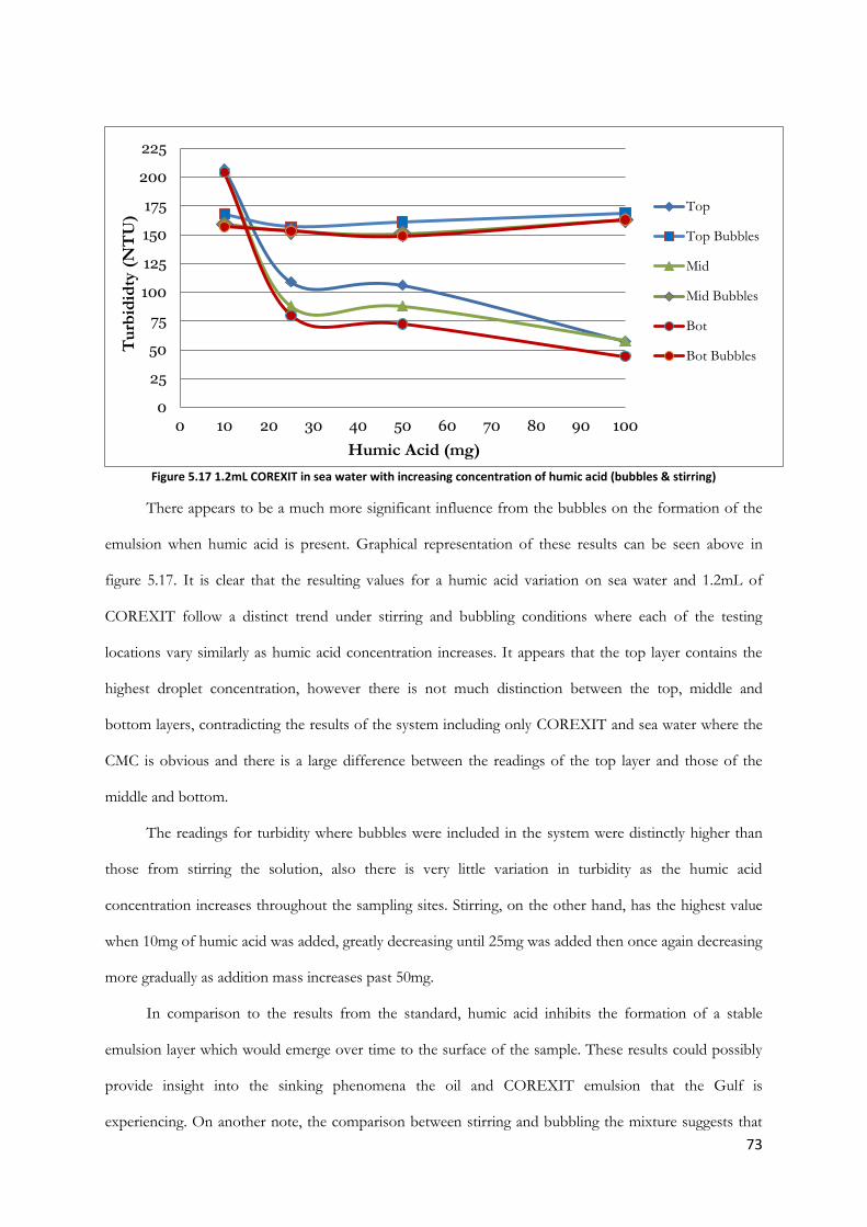
73
Figure 5.17 1.2mL COREXIT in sea water with increasing concentration of humic acid (bubbles & stirring)
There appears to be a much more significant influence from the bubbles on the formation of the
emulsion when humic acid is present. Graphical representation of these results can be seen above in
figure 5.17. It is clear that the resulting values for a humic acid variation on sea water and 1.2mL of
COREXIT follow a distinct trend under stirring and bubbling conditions where each of the testing
locations vary similarly as humic acid concentration increases. It appears that the top layer contains the
highest droplet concentration, however there is not much distinction between the top, middle and
bottom layers, contradicting the results of the system including only COREXIT and sea water where the
CMC is obvious and there is a large difference between the readings of the top layer and those of the
middle and bottom.
The readings for turbidity where bubbles were included in the system were distinctly higher than
those from stirring the solution, also there is very little variation in turbidity as the humic acid
concentration increases throughout the sampling sites. Stirring, on the other hand, has the highest value
when 10mg of humic acid was added, greatly decreasing until 25mg was added then once again decreasing
more gradually as addition mass increases past 50mg.
In comparison to the results from the standard, humic acid inhibits the formation of a stable
emulsion layer which would emerge over time to the surface of the sample. These results could possibly
provide insight into the sinking phenomena the oil and COREXIT emulsion that the Gulf is
experiencing. On another note, the comparison between stirring and bubbling the mixture suggests that
0
25
50
75
100
125
150
175
200
225
0 10 20 30 40 50 60 70 80 90 100
Tu
rbid
idty
(N
TU
)
Humic Acid (mg)
Top
Top Bubbles
Mid
Mid Bubbles
Bot
Bot Bubbles
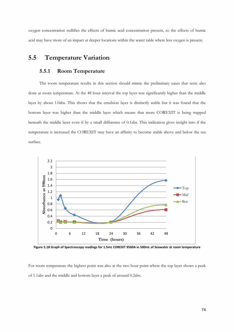
74
oxygen concentration nullifies the effects of humic acid concentration present, so the effects of humic
acid may have more of an impact at deeper locations within the water table where less oxygen is present.
5.5 Temperature Variation 5.5.1 Room Temperature The room temperature results in this section should mimic the preliminary cases that were also
done at room temperature. At the 48 hour interval the top layer was significantly higher than the middle
layer by about 1.0abs. This shows that the emulsion layer is distinctly stable but it was found that the
bottom layer was higher than the middle layer which means that more COREXIT is being trapped
beneath the middle layer even if by a small difference of 0.1abs. This indication gives insight into if the
temperature is increased the COREXIT may have an affinity to become stable above and below the sea
surface.
Figure 5.18 Graph of Spectroscopy readings for 1.5mL COREXIT 9500A in 500mL of Seawater at room temperature
For room temperature the highest point was also at the two hour point where the top layer shows a peak
of 1.1abs and the middle and bottom layer a peak of around 0.2abs.
0
0.2
0.4
0.6
0.8
1
1.2
1.4
1.6
1.8
2
2.2
0 6 12 18 24 30 36 42 48
Ab
sorb
an
ce a
t 590n
m
Time (hours)
Top
Mid
Bot
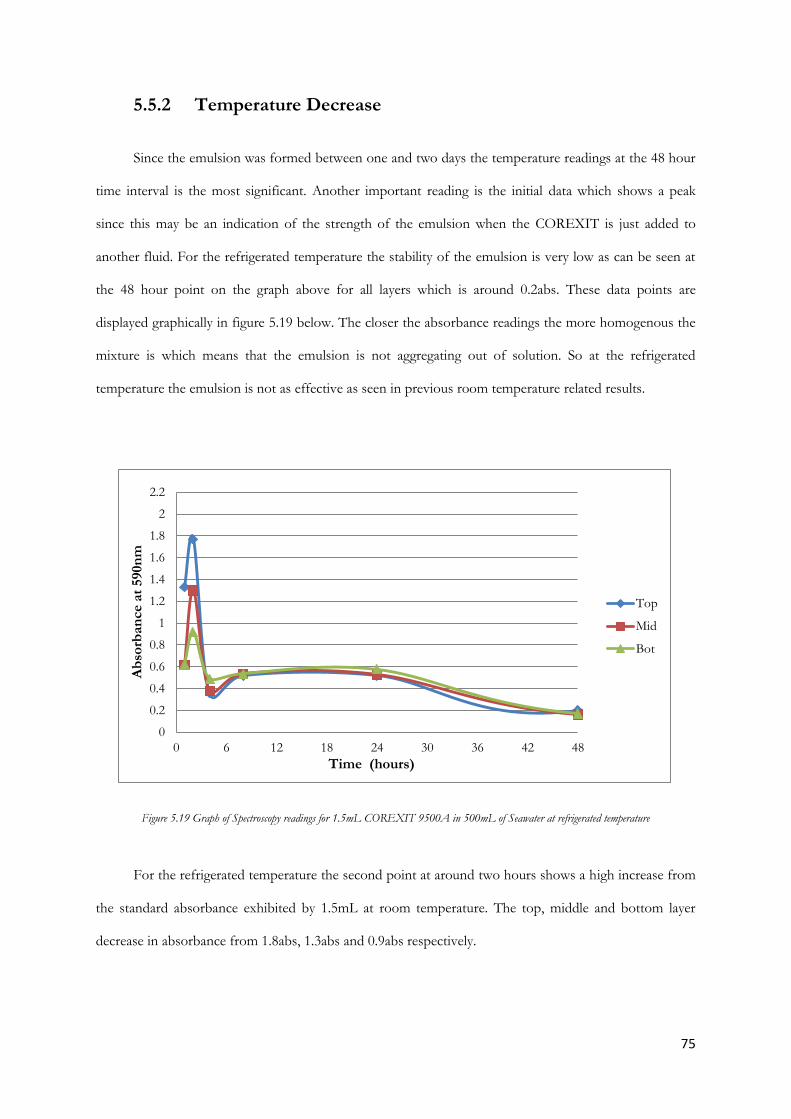
75
5.5.2 Temperature Decrease
Since the emulsion was formed between one and two days the temperature readings at the 48 hour
time interval is the most significant. Another important reading is the initial data which shows a peak
since this may be an indication of the strength of the emulsion when the COREXIT is just added to
another fluid. For the refrigerated temperature the stability of the emulsion is very low as can be seen at
the 48 hour point on the graph above for all layers which is around 0.2abs. These data points are
displayed graphically in figure 5.19 below. The closer the absorbance readings the more homogenous the
mixture is which means that the emulsion is not aggregating out of solution. So at the refrigerated
temperature the emulsion is not as effective as seen in previous room temperature related results.
Figure 5.19 Graph of Spectroscopy readings for 1.5mL COREXIT 9500A in 500mL of Seawater at refrigerated temperature
For the refrigerated temperature the second point at around two hours shows a high increase from
the standard absorbance exhibited by 1.5mL at room temperature. The top, middle and bottom layer
decrease in absorbance from 1.8abs, 1.3abs and 0.9abs respectively.
0
0.2
0.4
0.6
0.8
1
1.2
1.4
1.6
1.8
2
2.2
0 6 12 18 24 30 36 42 48
Ab
sorb
an
ce a
t 590n
m
Time (hours)
Top
Mid
Bot
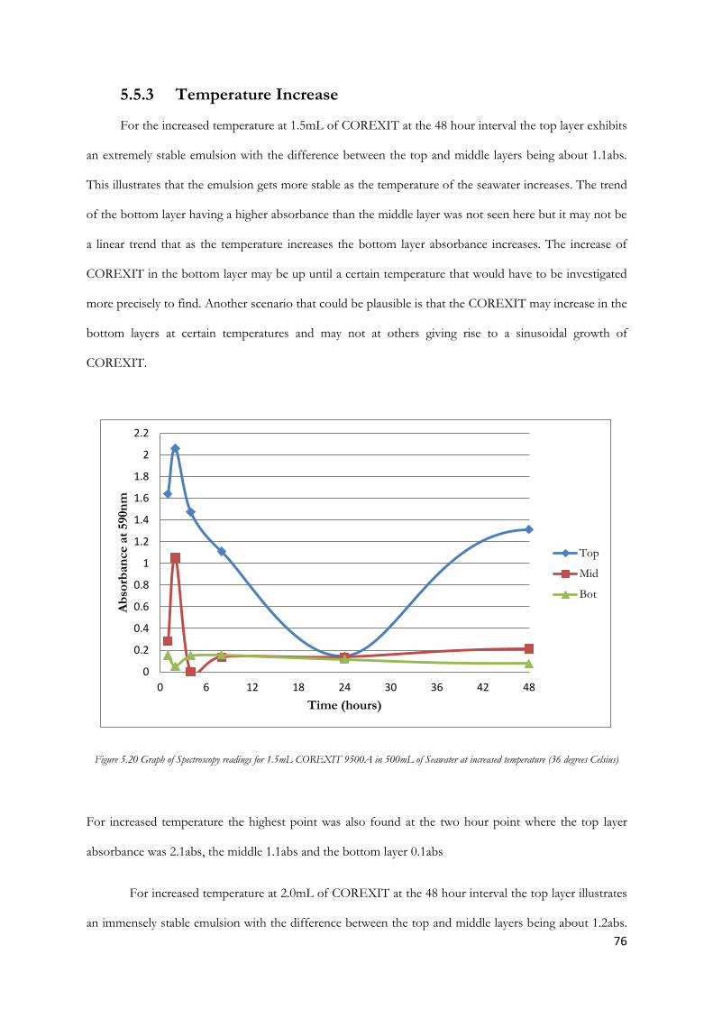
76
5.5.3 Temperature Increase
For the increased temperature at 1.5mL of COREXIT at the 48 hour interval the top layer exhibits
an extremely stable emulsion with the difference between the top and middle layers being about 1.1abs.
This illustrates that the emulsion gets more stable as the temperature of the seawater increases. The trend
of the bottom layer having a higher absorbance than the middle layer was not seen here but it may not be
a linear trend that as the temperature increases the bottom layer absorbance increases. The increase of
COREXIT in the bottom layer may be up until a certain temperature that would have to be investigated
more precisely to find. Another scenario that could be plausible is that the COREXIT may increase in the
bottom layers at certain temperatures and may not at others giving rise to a sinusoidal growth of
COREXIT.
Figure 5.20 Graph of Spectroscopy readings for 1.5mL COREXIT 9500A in 500mL of Seawater at increased temperature (36 degrees Celsius)
For increased temperature the highest point was also found at the two hour point where the top layer
absorbance was 2.1abs, the middle 1.1abs and the bottom layer 0.1abs
For increased temperature at 2.0mL of COREXIT at the 48 hour interval the top layer illustrates
an immensely stable emulsion with the difference between the top and middle layers being about 1.2abs.
0
0.2
0.4
0.6
0.8
1
1.2
1.4
1.6
1.8
2
2.2
0 6 12 18 24 30 36 42 48
Ab
sorb
an
ce a
t 590n
m
Time (hours)
Top
Mid
Bot

77
The increase in COREXIT at increased temperature increased the stability of the emulsion but this
cannot be assumed to be true as only one increase was done at increased temperature by a difference of
0.5mL of COREXIT. However the results do validate that the bottom layer does not have a higher
absorbance than the middle layer because the difference between the two layers is increased from 0.1abs
at 1.5mL at increased temperature to 0.3abs at 2.0mL at increased temperature.
Figure 5.21 Graph of Spectroscopy readings for 2.0mL COREXIT 9500A in 500mL of Seawater at increased temperature (36 degrees Celsius)
For increased temperature at 2.0mL of COREXIT the highest point is shown by the 48 hour point but
for the initial readings the two hour point was once again the highest with the top layer absorbance being
1.6abs and the middle and bottom layer being 0.2abs.
If the max absorbance does indicate the strength of emulsion when it is initially added to another
fluid then the increased temperature environment may be the best atmosphere to apply the COREXIT to
generate the best outcome. Since it does have the highest initial absorbance level recorded it may cause
the fluid’s surface tension to lessen faster causing easier dispersion.
0
0.2
0.4
0.6
0.8
1
1.2
1.4
1.6
1.8
2
2.2
0 6 12 18 24 30 36 42 48
Ab
sorb
an
ce a
t 590n
m
Time (hours)
Top
Mid
Bot
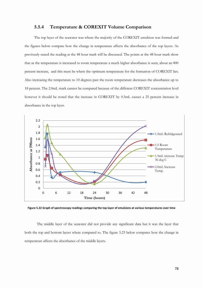
78
5.5.4 Temperature & COREXIT Volume Comparison The top layer of the seawater was where the majority of the COREXIT emulsion was formed and
the figures below compare how the change in temperature affects the absorbance of the top layers. As
previously stated the reading at the 48 hour mark will be discussed. The points at the 48 hour mark show
that as the temperature is increased to room temperature a much higher absorbance is seen, about an 800
percent increase, and this must be where the optimum temperature for the formation of COREXIT lies.
Also increasing the temperature to 10 degrees past the room temperature decreases the absorbance up to
18 percent. The 2.0mL mark cannot be compared because of the different COREXIT concentration level
however it should be noted that the increase in COREXIT by 0.5mL causes a 25 percent increase in
absorbance in the top layer.
Figure 5.22 Graph of spectroscopy readings comparing the top layer of emulsions at various temperatures over time
The middle layer of the seawater did not provide any significant data but it was the layer that
both the top and bottom layers where compared to. The figure 5.23 below compares how the change in
temperature affects the absorbance of the middle layers.
0
0.2
0.4
0.6
0.8
1
1.2
1.4
1.6
1.8
2
2.2
0 6 12 18 24 30 36 42 48
Ab
sorb
an
ce a
t 590n
m
Time (hours)
1.5mL Refridgerated
1.5 RoomTemperature
1.5mL increase Temp36 deg C
2.0mL IncreaseTemp.
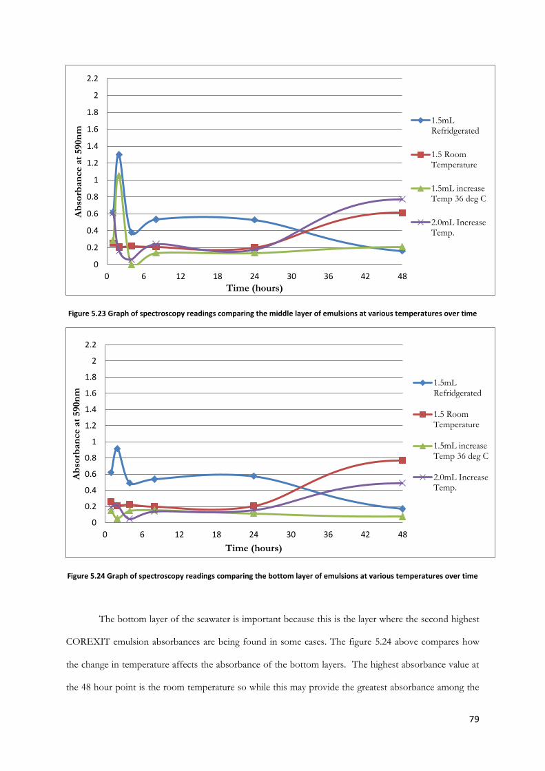
79
Figure 5.23 Graph of spectroscopy readings comparing the middle layer of emulsions at various temperatures over time
Figure 5.24 Graph of spectroscopy readings comparing the bottom layer of emulsions at various temperatures over time
The bottom layer of the seawater is important because this is the layer where the second highest
COREXIT emulsion absorbances are being found in some cases. The figure 5.24 above compares how
the change in temperature affects the absorbance of the bottom layers. The highest absorbance value at
the 48 hour point is the room temperature so while this may provide the greatest absorbance among the
0
0.2
0.4
0.6
0.8
1
1.2
1.4
1.6
1.8
2
2.2
0 6 12 18 24 30 36 42 48
Ab
sorb
an
ce a
t 590n
m
Time (hours)
1.5mLRefridgerated
1.5 RoomTemperature
1.5mL increaseTemp 36 deg C
2.0mL IncreaseTemp.
0
0.2
0.4
0.6
0.8
1
1.2
1.4
1.6
1.8
2
2.2
0 6 12 18 24 30 36 42 48
Ab
sorb
an
ce a
t 590n
m
Time (hours)
1.5mLRefridgerated
1.5 RoomTemperature
1.5mL increaseTemp 36 deg C
2.0mL IncreaseTemp.
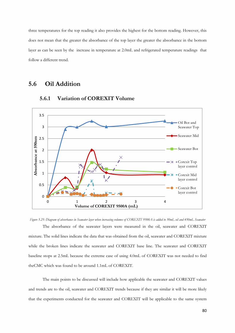
80
three temperatures for the top reading it also provides the highest for the bottom reading. However, this
does not mean that the greater the absorbance of the top layer the greater the absorbance in the bottom
layer as can be seen by the increase in temperature at 2.0mL and refrigerated temperature readings that
follow a different trend.
5.6 Oil Addition
5.6.1 Variation of COREXIT Volume
Figure 5.25: Diagram of absorbance in Seawater layer when increasing volumes of COREXIT 9500A is added to 50mL oil and 450mL Seawater
The absorbance of the seawater layers were measured in the oil, seawater and COREXIT
mixture. The solid lines indicate the data that was obtained from the oil, seawater and COREXIT mixture
while the broken lines indicate the seawater and COREXIT base line. The seawater and COREXIT
baseline stops at 2.5mL because the extreme case of using 4.0mL of COREXIT was not needed to find
theCMC which was found to be around 1.1mL of COREXIT.
The main points to be discussed will include how applicable the seawater and COREXIT values
and trends are to the oil, seawater and COREXIT trends because if they are similar it will be more likely
that the experiments conducted for the seawater and COREXIT will be applicable to the same system
0
0.5
1
1.5
2
2.5
3
3.5
0 1 2 3 4
Ab
sorb
an
ce a
t 590n
m
Volume of COREXIT 9500A (mL)
Oil Bot andSeawater Top
Seawater Mid
Seawater Bot
Corexit Toplayer control
Corexit Midlayer control
Corexit Botlayer control
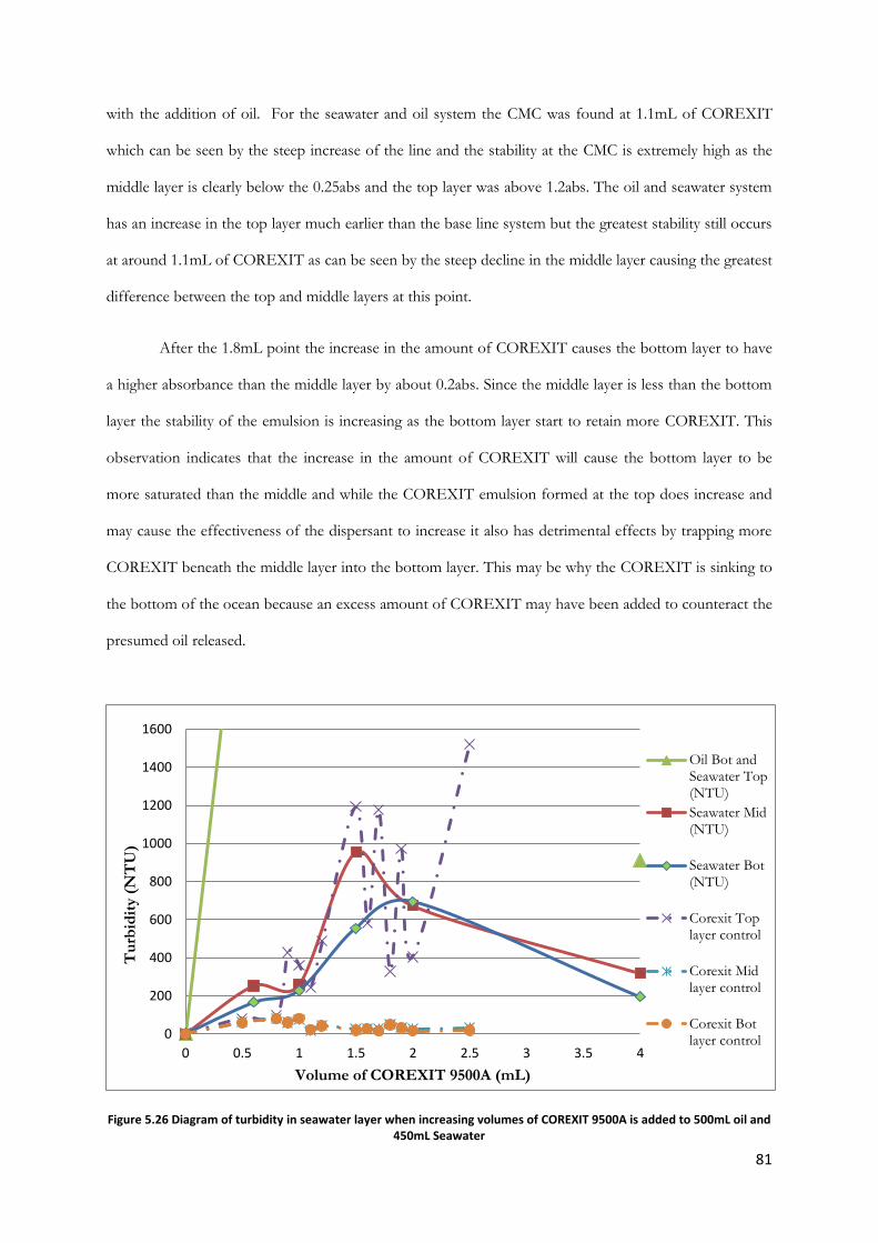
81
with the addition of oil. For the seawater and oil system the CMC was found at 1.1mL of COREXIT
which can be seen by the steep increase of the line and the stability at the CMC is extremely high as the
middle layer is clearly below the 0.25abs and the top layer was above 1.2abs. The oil and seawater system
has an increase in the top layer much earlier than the base line system but the greatest stability still occurs
at around 1.1mL of COREXIT as can be seen by the steep decline in the middle layer causing the greatest
difference between the top and middle layers at this point.
After the 1.8mL point the increase in the amount of COREXIT causes the bottom layer to have
a higher absorbance than the middle layer by about 0.2abs. Since the middle layer is less than the bottom
layer the stability of the emulsion is increasing as the bottom layer start to retain more COREXIT. This
observation indicates that the increase in the amount of COREXIT will cause the bottom layer to be
more saturated than the middle and while the COREXIT emulsion formed at the top does increase and
may cause the effectiveness of the dispersant to increase it also has detrimental effects by trapping more
COREXIT beneath the middle layer into the bottom layer. This may be why the COREXIT is sinking to
the bottom of the ocean because an excess amount of COREXIT may have been added to counteract the
presumed oil released.
Figure 5.26 Diagram of turbidity in seawater layer when increasing volumes of COREXIT 9500A is added to 500mL oil and 450mL Seawater
0
200
400
600
800
1000
1200
1400
1600
0 0.5 1 1.5 2 2.5 3 3.5 4
Tu
rbid
ity (
NT
U)
Volume of COREXIT 9500A (mL)
Oil Bot andSeawater Top(NTU)
Seawater Mid(NTU)
Seawater Bot(NTU)
Corexit Toplayer control
Corexit Midlayer control
Corexit Botlayer control
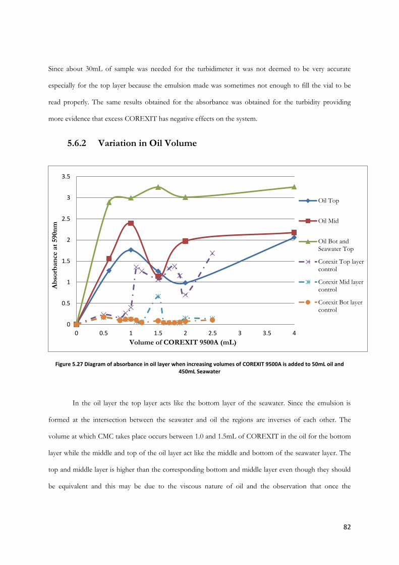
82
Since about 30mL of sample was needed for the turbidimeter it was not deemed to be very accurate
especially for the top layer because the emulsion made was sometimes not enough to fill the vial to be
read properly. The same results obtained for the absorbance was obtained for the turbidity providing
more evidence that excess COREXIT has negative effects on the system.
5.6.2 Variation in Oil Volume
Figure 5.27 Diagram of absorbance in oil layer when increasing volumes of COREXIT 9500A is added to 50mL oil and 450mL Seawater
In the oil layer the top layer acts like the bottom layer of the seawater. Since the emulsion is
formed at the intersection between the seawater and oil the regions are inverses of each other. The
volume at which CMC takes place occurs between 1.0 and 1.5mL of COREXIT in the oil for the bottom
layer while the middle and top of the oil layer act like the middle and bottom of the seawater layer. The
top and middle layer is higher than the corresponding bottom and middle layer even though they should
be equivalent and this may be due to the viscous nature of oil and the observation that once the
0
0.5
1
1.5
2
2.5
3
3.5
0 0.5 1 1.5 2 2.5 3 3.5 4
Ab
sorb
an
ce a
t 590n
m
Volume of COREXIT 9500A (mL)
Oil Top
Oil Mid
Oil Bot andSeawater Top
Corexit Top layercontrol
Corexit Mid layercontrol
Corexit Bot layercontrol
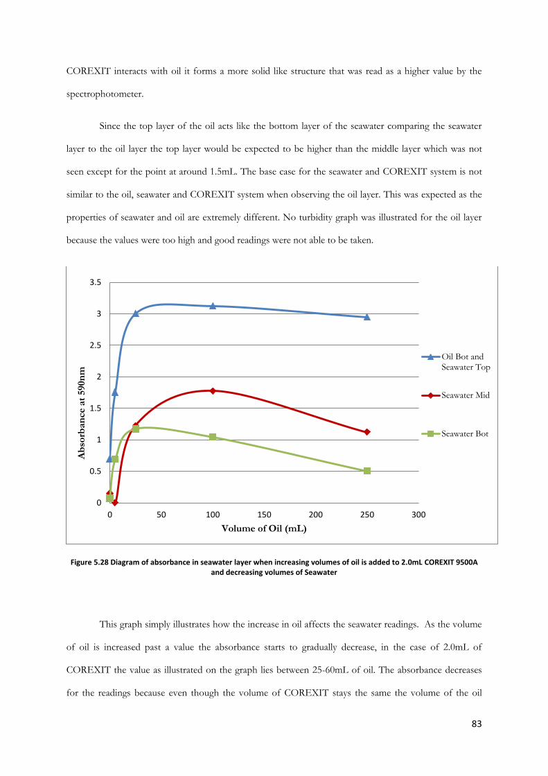
83
COREXIT interacts with oil it forms a more solid like structure that was read as a higher value by the
spectrophotometer.
Since the top layer of the oil acts like the bottom layer of the seawater comparing the seawater
layer to the oil layer the top layer would be expected to be higher than the middle layer which was not
seen except for the point at around 1.5mL. The base case for the seawater and COREXIT system is not
similar to the oil, seawater and COREXIT system when observing the oil layer. This was expected as the
properties of seawater and oil are extremely different. No turbidity graph was illustrated for the oil layer
because the values were too high and good readings were not able to be taken.
Figure 5.28 Diagram of absorbance in seawater layer when increasing volumes of oil is added to 2.0mL COREXIT 9500A and decreasing volumes of Seawater
This graph simply illustrates how the increase in oil affects the seawater readings. As the volume
of oil is increased past a value the absorbance starts to gradually decrease, in the case of 2.0mL of
COREXIT the value as illustrated on the graph lies between 25-60mL of oil. The absorbance decreases
for the readings because even though the volume of COREXIT stays the same the volume of the oil
0
0.5
1
1.5
2
2.5
3
3.5
0 50 100 150 200 250 300
Ab
sorb
an
ce a
t 590n
m
Volume of Oil (mL)
Oil Bot andSeawater Top
Seawater Mid
Seawater Bot

84
which is denser than the emulsion increases and this causes the volume of the COREXIT layer within the
oil to be stretched throughout a larger volume of oil decreasing the amount at the interface which
decreases the absorbance that can read in the seawater layer.
85
Chapter 6: Conclusions
Micellization occurs at the CMC at the same concentration of COREXIT 9500A when salt water
is more than 50 percent by volume. As salinity increases the extent of micelle formation increases which
is supported by the findings in section 5.2 above where absorbance increases as salt water concentration
increases. This determination proves that the emulsion formed at higher salinity is more stable than that
where the solution is diluted by deionized water.
As the concentration of the COREXIT is increased the ability for the COREXIT to form a
stable emulsion also increases. As the volume of COREXIT increases the absorbance of COREXIT in
the bottom layer also increases. This means that more of the COREXIT emulsion is being trapped in the
bottom layer which may be one of the main reasons why COREXIT is descending in the Gulf of Mexico
instead of dispersing the oil and performing ideally.
Sand added before and after the COREXIT was added simulates sand above and below the
emulsion layer and showed that for the emulsion at the top layer adding the sand after the COREXIT
yielded higher absorbance. For the bottom layer higher absorbance were recorded for adding the sand
before the COREXIT.
Results from the humic acid experiments suggest that organic matter limits the formation of an
emulsion, particularly as the concentration of these particulates increases. The addition of humic material
produced results of a more uniform emulsion throughout the beaker which leads to the conclusion that
the extent of micelle formation is limited.
The addition of air bubbles in the samples of deionized and sea water with COREXIT proved
insignificant, producing similar reading to the control. Alternatively, the bubbles produced more of an
effect on a salt water solution containing humic acid and COREXIT. The air within the humic acid
solution appears to further inhibit the separation of the emulsion phase resulting in a uniform mixture
and minimal, if any, micelle formation.
86
The increase in temperature increases the stability of the emulsion due to the increasing
difference between the middle and top layers. This shows that increasing the temperature causes the
COREXIT to perform more effectively. Therefore depending on what the temperature was in the Gulf
of Mexico when the COREXIT was added determines how well it acted as a surfactant. Since the
application of COREXIT was done at sea level and sub-sea level, varying degree of effectiveness can be
expected especially since the deeper the COREXIT was applied the colder the mixing conditions.
At lower temperatures micellization does not seem to occur and this could have increased the
COREXIT concentration being found throughout the depths of the sea. If the conditions were cold
upon application of COREXIT the emulsion would not form and the COREXIT would be dispersed
homogenously as seen at the refrigerated temperature results. Room Temperature also produced the most
significant increase in top layer absorbance and therefore could potentially be the optimum temperature
at which COREXIT was meant to be applied.
The addition of oil to the seawater and COREXIT system produces similar trends for the CMC
as the seawater and COREXIT alone in the seawater layer. In the oil layer of the oil, seawater and
COREXIT mixture the inverse trend is observed for the CMC. The bottom layer of the seawater in the
oil, seawater and COREXIT mixture is greater than the middle layer at COREXIT values past 1.8mL
which means that adding excessive volumes of COREXIT actually causes more COREXIT to be trapped
within the bottom layer of the seawater. This means that applying a large quantity of COREXIT to
disperse an unknown large quantity of oil may have led to the sinking of COREXIT to the bottom of the
Gulf of Mexico.
Overall many factors affected how the COREXIT emulsion was formed and the overall stability
of the COREXIT emulsion is directly dependent on some of the factors tested in this experiment. The
factors that strongly affect the formation of the COREXIT emulsion include if oil or another viscous
fluid is added and the volume of that viscous fluid added, temperature, salinity, humic acid, the addition
of smaller sand particles. Other minor factors include the amount of air bubbles that comes in contact
with the COREXIT emulsion layer and the addition of large sand particles.
87
Chapter 7: Recommendations
Our first recommendation relates to the use of COREXIT 9500A in the Gulf of Mexico in
regards to proper use of the material, which includes methods to introduce the COREXIT to an
area contaminated by an oil spill as well as validating that the dispersant is the proper material for
optimal results. Throughout our research it has become apparent that the underwater injection
of the COREXIT at the base of the Deepwater Horizon oil rig resulted in unexpected emulsion
behavior due to several factors including temperature and dissolved particles. Surface application
truly appears to be the best option as the conditions at this point are optimal for droplet
breakup.
Further experimentation is suggested to explore different properties of the COREXIT with
similar permutations as to the ones we chose for the project. Specifically, more surface chemistry
of the emulsion formed should be investigated in relation to electrical potential and possible
functional groups which are expelled with chemicals during an oil spill. More advanced
technology would be necessary for these experiments but would provide valuable insight on the
microscopic workings of the emulsion which is formed by the COREXIT. On another note,
other dispersants could also be investigated and compared to COREXIT in regards to how they
may behave similarly or contrary when our selected variables are present in the system. This
could provide interesting findings on whether one dispersant is more appropriate than another
and why.
In regards to our specific experiments, more investigation into the kinetics of the formation
and decomposition of the microemusion resulting from the addition of COREXIT would be
valuable to the study of the stability of the sample. Similarly, replications should be performed to
validate the results we have explained above, although we were able to replicate some initial
experiments, time did not permit replication of each.
Finally, experimentation on a more appropriate model of the Gulf conditions should be
pursued. This would consist of working with actual samples of sea water from the Gulf of
Mexico, and with the proper technology, temperature could be held constant to more

88
appropriately simulate the conditions of the water affected by the Deepwater Horizon oil spill.
Another potentially interesting group of experiments could be performed to simulate the surface
of the ocean waters where there is constant, turbid movement and other factors come into play
such as weather and mechanical disturbances. In addition, a larger scale model would be more
helpful in simulating the actual occurrences within an ocean system, and also provide a larger
testing sample which could inevitably simplify removing the samples from the various locations
within the solution.
89
References A. George-Ares, J. R. Clark, Aquatic toxicity of two COREXIT(R) dispersants, Chemosphere, Volume
40, Issue 8, April 2000, Pages 897-906 (http://www.sciencedirect.com/science/article/B6V74-
3YGDD0T-28/2/8cf0ec1576d4b7347ff4cc88aa006abc)
"Amazing Images Capture Tragedy of Gulf Oil Spill." limewedge. N.p., 23 May 2010. Web. 27 May 2011.
<limewedge.net/amazing-images-capture-tragedy-of-gulf-oil-spill>.
Amendola, Kim. "Coastal Conservation Association." Coastal Conservation Association (CCA). United States
Department of Commerce, 22 Oct. 2010. Web. 28 Apr. 2011.
<http://www.joincca.org/media%20room/Gulf/oil_opening102210.htm
Bowyer, R. Terry, et al. "Effects of the Exxon Valdez Oil Spill on River Otters: Injury and Recovery of a
Sentinel Species." Wildlife Monographs.153, Effects of the Exxon Valdez Oil Spill on River Otters:
Injury and Recovery of a Sentinel Species (2003): pp. 1-53. Web.
Braddock, JF. . J. E. Lindstroamn, DE . J. Brown1. 995. Distribution of hydrocarbon degrading
microorganisms in sediments from Prince William Sound, Alaska, following the Exxon Valdez oil
spill. Marine Pollution Bulletin, Volume 30, Issue 2, February 1995, Pages 125-132,
(http://www.sciencedirect.com/science/article/B6V6N-3YMFRFM-
3F/2/6bcfc8bd02daa9abbb10658f29ac0546)
Campbell, D., Cox, D., Crum, J., Foster, F., Christie, P., Brewster, D.1993. Initial effects of the grounding
of the tanker Braer on health in shetland. Br. Med. J. 307, 1251–1255
"COREXIT Ingredients." Essential Expertise for Water, Energy and Air - Nalco Company Homepage. Web. 28
Apr. 2011. <http://www.nalco.com/applications/4297.htm>.
"Deeper Insights: Researching the Spill Under the Sea : NOAA Gulf Spill Restoration." NOAA Gulf
Spill Restoration. NOAA Gulf Spill Restoration, 3 Nov. 2010. Web. 28 Apr. 2011.
<http://www.gulfspillrestoration.noaa.gov/2010/11/deeper-insights-researching-the-spill-under-
the-sea/>.
E. A. Tsocalis, T. Kowenhoven, A. Perakis, Mar. Technol. Sname, News 31 (1994) 79–93.
90
E. Vergetis, Oil pollution in Greek seas and spillconfrontation means-methods, National Technical
University of Athens, Greece, 2002.
Elimelech, M., et. al; Particle Deposition & Aggregation: Measurement, Modelling and Simulation Published by
Butterworth-Heinemann Ltd. 1995, Oxford.
Etkin, D.S., 1999. Oil Spill Dispersants: From Technology to Policy. Cutter Information Corp.,
Arlington, MA
Fingas, Merv. "Oil Spill Dispersion Stability and." Oil Spill Dispersion Stability and - (2007): 6. Print.
Gillis, Justin, and John Rudolf. "Gulf Oil Plume Is Not Breaking Down Fast, Study Says -
NYTimes.com." The New York Times - Breaking News, World News & Multimedia. N.p., 19 Aug. 2010.
Web. 28 Apr. 2011.
<http://www.nytimes.com/2010/08/20/science/earth/20plume.html_r=1&ref=gulf_of_mexico_
2010>.
Guard, U.S. Coast. "Pollution Response unit deploys containment boom | Flickr - Photo Sharing!." Flickr
- Photo Sharing. U.S Navy, 4 May 2010. Web. 29 Apr. 2011. <http://www.flickr.com/photos/coast
"Gulf of Mexico Deepwater Horizon Oil Spill (2010) - The New York Times." Times Topics. The New
York Times, 25 Apr. 2011. Web. 28 Apr. 2011. <http://topics.nytimes.com/top/
Israelachvili, Jacob Inetermolecular & Surface Forces 2nd Edition Achademic Press, San Diego, California 1992
Jackson, J. B. C., et al. "Ecological Effects of a Major Oil Spill on Panamanian Coastal Marine
Communities." Science 243.4887 (1989): pp. 37-44. Web.
Jones, Malcolm N. Micelles, Monolayers, and Biomembranes A John Wiley & Sons, Inc. Publication, New
York, NY 1995.
Kester, Dana R., et al. "Preparation of Artificial Seawater." Limnology and Oceanography 12.1 (1967): pp.
176-179. Web.
Laurd, Andl . Haldorson, 1996 Coastal habitat studies: the effect of the Exxon Valdez Oil spill on
shallow subtidal fishes in Prince William Sound.American Fisheries Society Symposia1 8:659-670.
Lee, K., et al. "Microbial Response to Crude Oil and COREXIT 9527: SEAFLUXES Enclosure Study."
Microbial ecology 11.4 (1985): pp. 337-351. Web.
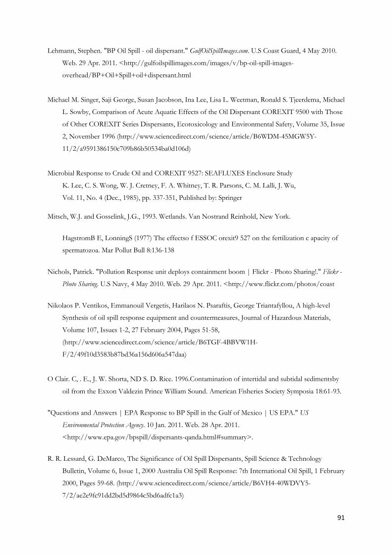
91
Lehmann, Stephen. "BP Oil Spill - oil dispersant." GulfOilSpillImages.com. U.S Coast Guard, 4 May 2010.
Web. 29 Apr. 2011. <http://gulfoilspillimages.com/images/v/bp-oil-spill-images-
overhead/BP+Oil+Spill+oil+dispersant.html
Michael M. Singer, Saji George, Susan Jacobson, Ina Lee, Lisa L. Weetman, Ronald S. Tjeerdema, Michael
L. Sowby, Comparison of Acute Aquatic Effects of the Oil Dispersant COREXIT 9500 with Those
of Other COREXIT Series Dispersants, Ecotoxicology and Environmental Safety, Volume 35, Issue
2, November 1996 (http://www.sciencedirect.com/science/article/B6WDM-45MGW5Y-
11/2/a9591386150c709b86b50534ba0d106d)
Microbial Response to Crude Oil and COREXIT 9527: SEAFLUXES Enclosure Study
K. Lee, C. S. Wong, W. J. Cretney, F. A. Whitney, T. R. Parsons, C. M. Lalli, J. Wu,
Vol. 11, No. 4 (Dec., 1985), pp. 337-351, Published by: Springer
Mitsch, W.J. and Gosselink, J.G., 1993. Wetlands. Van Nostrand Reinhold, New York.
HagstromB E, LonningS (1977) The effectso f ESSOC orexit9 527 on the fertilization c apacity of
spermatozoa. Mar Pollut Bull 8:136-138
Nichols, Patrick. "Pollution Response unit deploys containment boom | Flickr - Photo Sharing!." Flickr -
Photo Sharing. U.S Navy, 4 May 2010. Web. 29 Apr. 2011. <http://www.flickr.com/photos/coast
Nikolaos P. Ventikos, Emmanouil Vergetis, Harilaos N. Psaraftis, George Triantafyllou, A high-level
Synthesis of oil spill response equipment and countermeasures, Journal of Hazardous Materials,
Volume 107, Issues 1-2, 27 February 2004, Pages 51-58,
(http://www.sciencedirect.com/science/article/B6TGF-4BBVW1H-
F/2/49f10d3583b87bd36a156d606a547daa)
O Clair. C, . E., J. W. Shorta, ND S. D. Rice. 1996.Contamination of intertidal and subtidal sedimentsby
oil from the Exxon Valdezin Prince William Sound. American Fisheries Society Symposia 18:61-93.
"Questions and Answers | EPA Response to BP Spill in the Gulf of Mexico | US EPA." US
Environmental Protection Agency. 10 Jan. 2011. Web. 28 Apr. 2011.
<http://www.epa.gov/bpspill/dispersants-qanda.html#summary>.
R. R. Lessard, G. DeMarco, The Significance of Oil Spill Dispersants, Spill Science & Technology
Bulletin, Volume 6, Issue 1, 2000 Australia Oil Spill Response: 7th International Oil Spill, 1 February
2000, Pages 59-68. (http://www.sciencedirect.com/science/article/B6VH4-40WDVY5-
7/2/ae2e9fc91dd2bd5d9864c5bd6adfc1a3)

92
Scientists, Woods Hole. "Image : WHOI Scientists Map and Confirm Origin of Large, Underwater
Hydrocarbon Plume in Gulf : Deepwater Horizon Oil Spill Response." Woods Hole Oceanographic
Institute. Woods Hole Oceanographic Institute, 23 Feb. 2011. Web. 29 Apr. 2011.
<http://www.whoi.edu/dwhresponse/page.do?pid=43720&tid=441&cid=116978
Schramm, Laurier L. Emulsions: Fundamentals and Applications in the Petroleum Industry American Chemical
Society, Washington, DC 1992.
Sultan Ayoub Meo, Abdul Majeed Al-Drees, Imran M.U. Meo, Muslim M. Al-Saadi, Muhammad Abdul
Azeem, Lung function in subjects exposed to crude oil spill into sea water, Marine Pollution
Bulletin, Volume 56, Issue 1, January 2008, Pages 88-94,
(http://www.sciencedirect.com/science/article/B6V6N-4R70C2X-
1/2/9fe2891e1c1bc8c1b76a30ebfc947d22)
Venosa, A. D., and E. L. Holder. "Biodegradability of Dispersed Crude Oil at Two Different
Temperatures." Marine pollution bulletin 54.5 (2007): 545-53. Web.
Venosa, Albert D., Dennis W. King, and George A. Sorial. "The Baffled Flask Test for Dispersant
Effectiveness: A Round Robin Evaluation of Reproducibility and Repeatability." Spill Science &
Technology Bulletin 7.5-6 (2002): 299-308. Web.
Ventikos, Nikolaos P., et al. "A High-Level Synthesis of Oil Spill Response Equipment and
Countermeasures." Journal of hazardous materials 107.1-2 (2004): 51-8. Web.
Vidali, Roza et. all An Experimental and modeling study of humic acid concentration effect on H+Binding: Application
of the NICA-Donnan Model Journal of Colloid and Interface Science 2009
Witherington, Blair. "Gulf of Mexico oil spill turtle rescue | Photos | Chron.com - Houston Chronicle."
Houston news, entertainment, search and shopping | chron.com - Houston Chronicle. Florida Fish and Wildlife
Conservation Commission, 18 June 2010. Web. 29 Apr. 2011. <http://www.chron.com/business
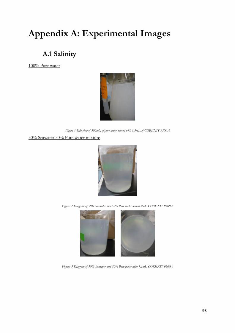
93
Appendix A: Experimental Images
A.1 Salinity
100% Pure water
Figure 1 Side view of 500mL of pure water mixed with 1.5mL of COREXIT 9500A
50% Seawater 50% Pure water mixture
Figure: 2 Diagram of 50% Seawater and 50% Pure water with 0.9mL COREXIT 9500A
Figure: 3 Diagram of 50% Seawater and 50% Pure water with 1.1mL COREXIT 9500A
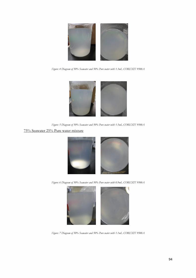
94
Figure: 4 Diagram of 50% Seawater and 50% Pure water with 1.3mL COREXIT 9500A
Figure: 5 Diagram of 50% Seawater and 50% Pure water with 1.5mL COREXIT 9500A
75% Seawater 25% Pure water mixture
Figure: 6 Diagram of 50% Seawater and 50% Pure water with 0.9mL COREXIT 9500A
Figure: 7 Diagram of 50% Seawater and 50% Pure water with 1.1mL COREXIT 9500A
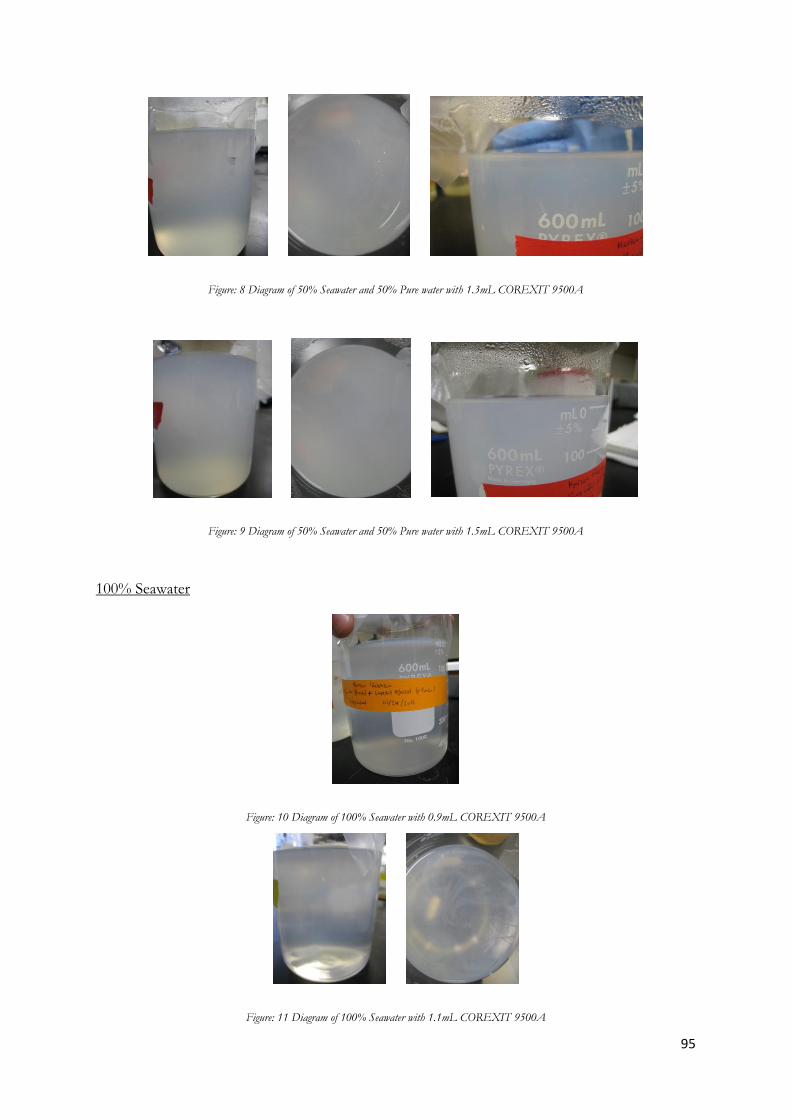
95
Figure: 8 Diagram of 50% Seawater and 50% Pure water with 1.3mL COREXIT 9500A
Figure: 9 Diagram of 50% Seawater and 50% Pure water with 1.5mL COREXIT 9500A
100% Seawater
Figure: 10 Diagram of 100% Seawater with 0.9mL COREXIT 9500A
Figure: 11 Diagram of 100% Seawater with 1.1mL COREXIT 9500A
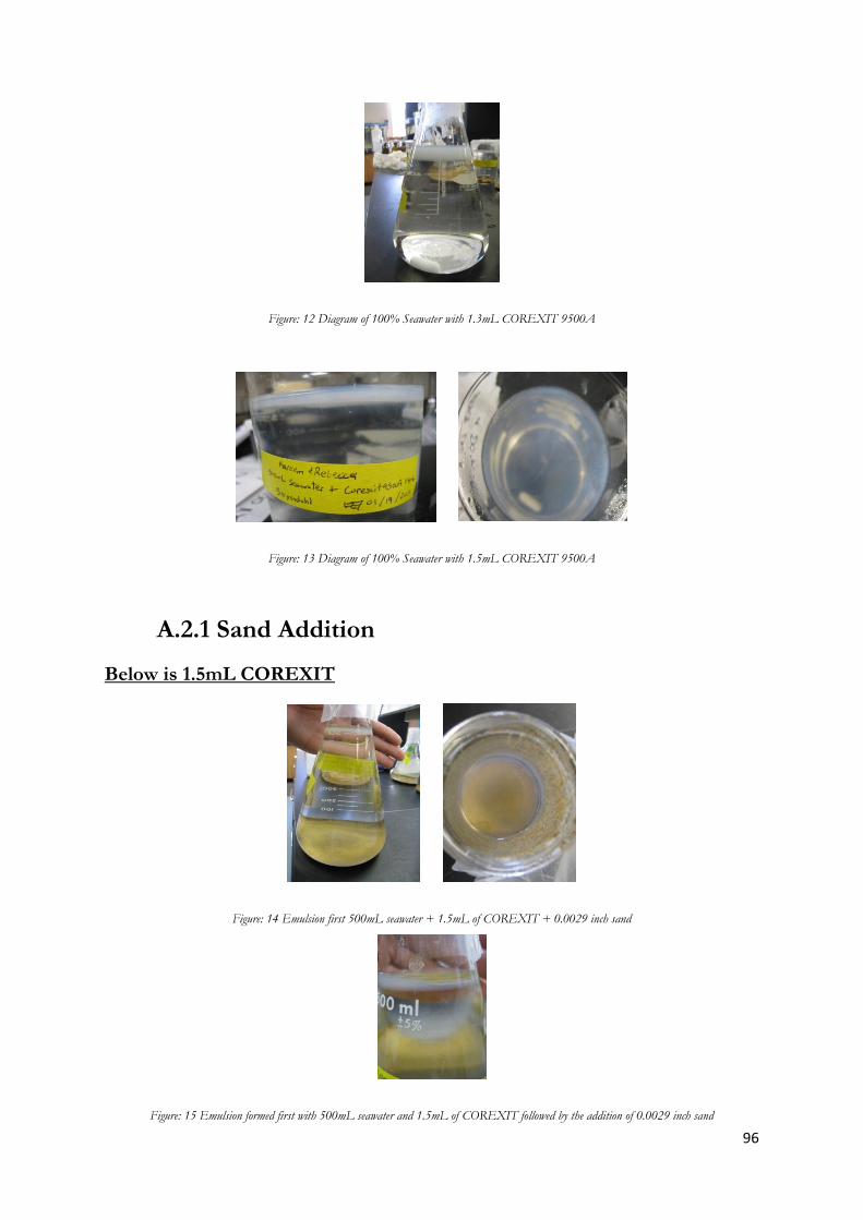
96
Figure: 12 Diagram of 100% Seawater with 1.3mL COREXIT 9500A
Figure: 13 Diagram of 100% Seawater with 1.5mL COREXIT 9500A
A.2.1 Sand Addition
Below is 1.5mL COREXIT
Figure: 14 Emulsion first 500mL seawater + 1.5mL of COREXIT + 0.0029 inch sand
Figure: 15 Emulsion formed first with 500mL seawater and 1.5mL of COREXIT followed by the addition of 0.0029 inch sand
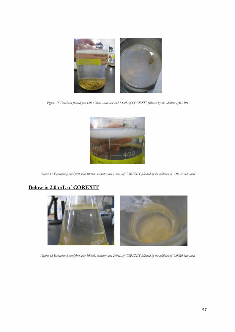
97
Figure: 16 Emulsion formed first with 500mL seawater and 1.5mL of COREXIT followed by the addition of 0.0394
Figure: 17 Emulsion formed first with 500mL seawater and 1.5mL of COREXIT followed by the addition of 0.0394 inch sand
Below is 2.0 mL of COREXIT
Figure: 18 Emulsion formed first with 500mL seawater and 2.0mL of COREXIT followed by the addition of 0.0029 inch sand
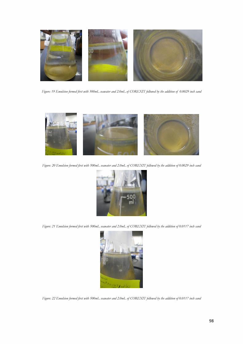
98
Figure: 19 Emulsion formed first with 500mL seawater and 2.0mL of COREXIT followed by the addition of 0.0029 inch sand
Figure: 20 Emulsion formed first with 500mL seawater and 2.0mL of COREXIT followed by the addition of 0.0029 inch sand
Figure: 21 Emulsion formed first with 500mL seawater and 2.0mL of COREXIT followed by the addition of 0.0117 inch sand
Figure: 22 Emulsion formed first with 500mL seawater and 2.0mL of COREXIT followed by the addition of 0.0117 inch sand
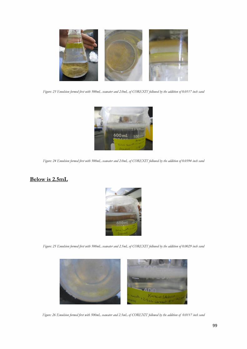
99
Figure: 23 Emulsion formed first with 500mL seawater and 2.0mL of COREXIT followed by the addition of 0.0117 inch sand
Figure: 24 Emulsion formed first with 500mL seawater and 2.0mL of COREXIT followed by the addition of 0.0394 inch sand
Below is 2.5mL
Figure: 25 Emulsion formed first with 500mL seawater and 2.5mL of COREXIT followed by the addition of 0.0029 inch sand
Figure: 26 Emulsion formed first with 500mL seawater and 2.5mL of COREXIT followed by the addition of 0.0117 inch sand
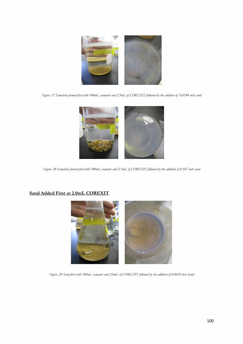
100
Figure: 27 Emulsion formed first with 500mL seawater and 2.5mL of COREXIT followed by the addition of 0.0394 inch sand
Figure: 28 Emulsion formed first with 500mL seawater and 2.5mL of COREXIT followed by the addition of 0.187 inch sand
Sand Added First at 2.0mL COREXIT
Figure: 29 Sand first with 500mL seawater and 2.0mL of COREXIT followed by the addition of 0.0029 inch Sand
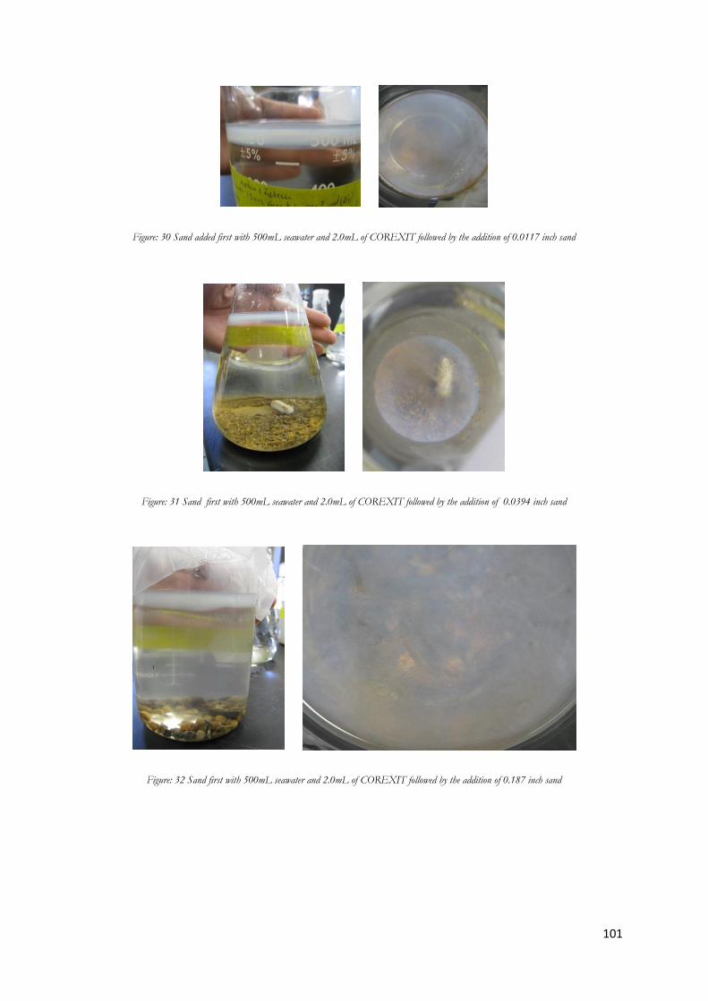
101
Figure: 30 Sand added first with 500mL seawater and 2.0mL of COREXIT followed by the addition of 0.0117 inch sand
Figure: 31 Sand first with 500mL seawater and 2.0mL of COREXIT followed by the addition of 0.0394 inch sand
Figure: 32 Sand first with 500mL seawater and 2.0mL of COREXIT followed by the addition of 0.187 inch sand
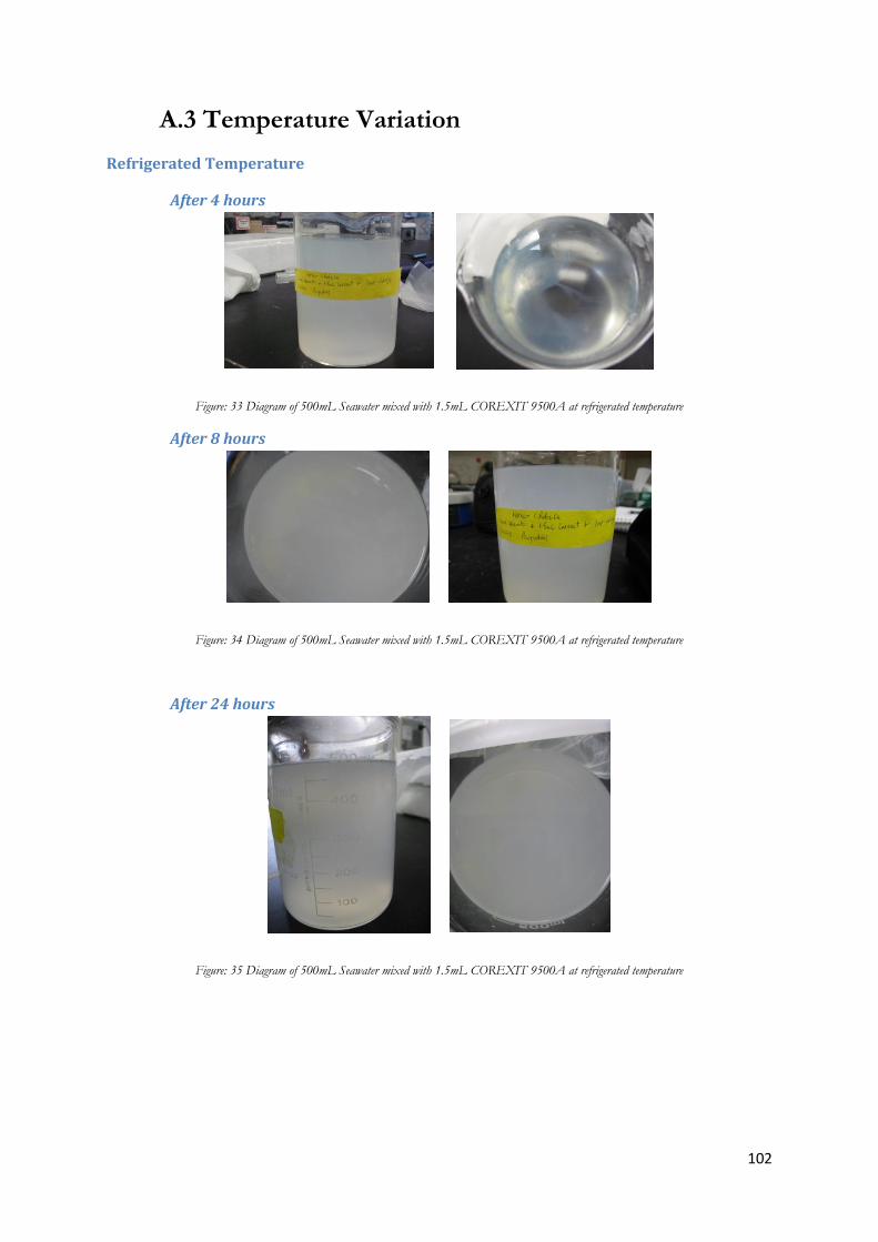
102
A.3 Temperature Variation
Refrigerated Temperature
After 4 hours
Figure: 33 Diagram of 500mL Seawater mixed with 1.5mL COREXIT 9500A at refrigerated temperature
After 8 hours
Figure: 34 Diagram of 500mL Seawater mixed with 1.5mL COREXIT 9500A at refrigerated temperature
After 24 hours
Figure: 35 Diagram of 500mL Seawater mixed with 1.5mL COREXIT 9500A at refrigerated temperature
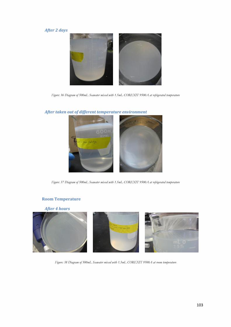
103
After 2 days
Figure: 36 Diagram of 500mL Seawater mixed with 1.5mL COREXIT 9500A at refrigerated temperature
After taken out of different temperature environment
Figure: 37 Diagram of 500mL Seawater mixed with 1.5mL COREXIT 9500A at refrigerated temperature
Room Temperature
After 4 hours
Figure: 38 Diagram of 500mL Seawater mixed with 1.5mL COREXIT 9500A at room temperature
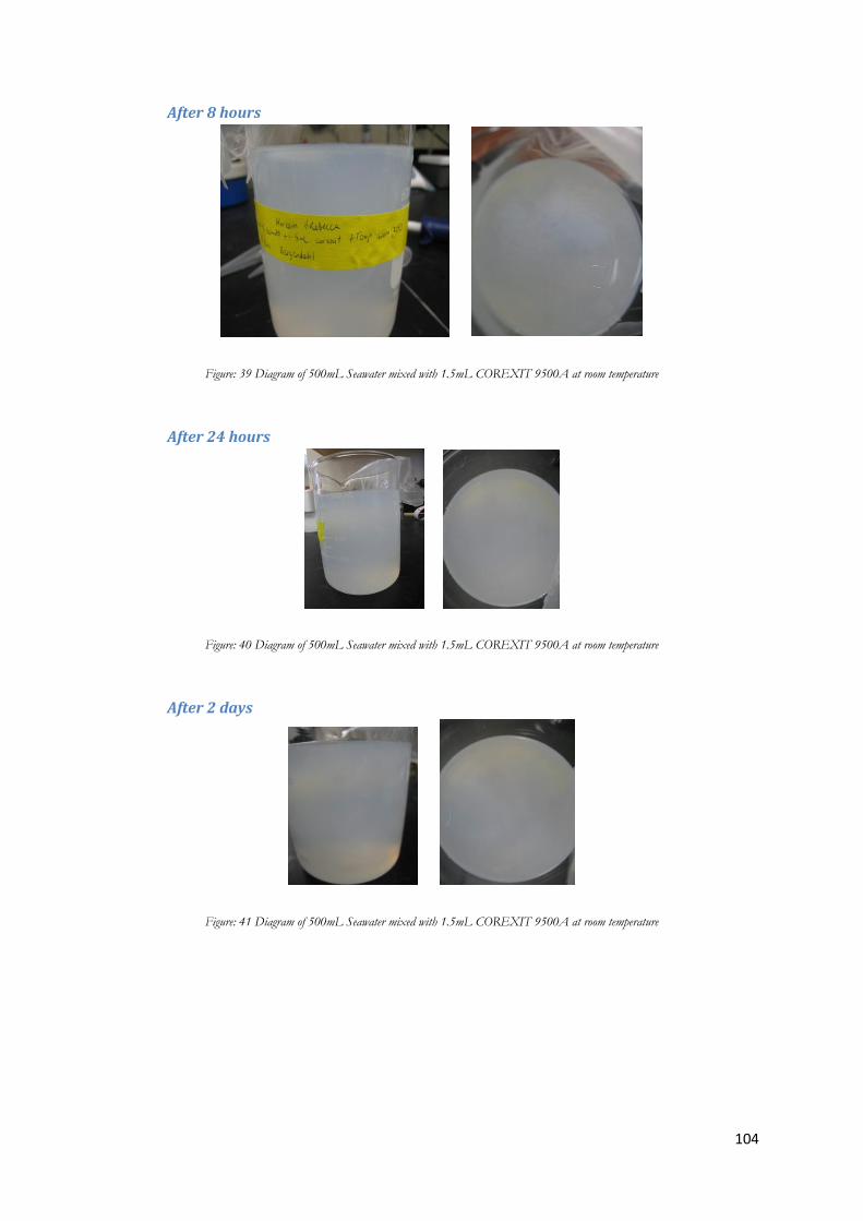
104
After 8 hours
Figure: 39 Diagram of 500mL Seawater mixed with 1.5mL COREXIT 9500A at room temperature
After 24 hours
Figure: 40 Diagram of 500mL Seawater mixed with 1.5mL COREXIT 9500A at room temperature
After 2 days
Figure: 41 Diagram of 500mL Seawater mixed with 1.5mL COREXIT 9500A at room temperature
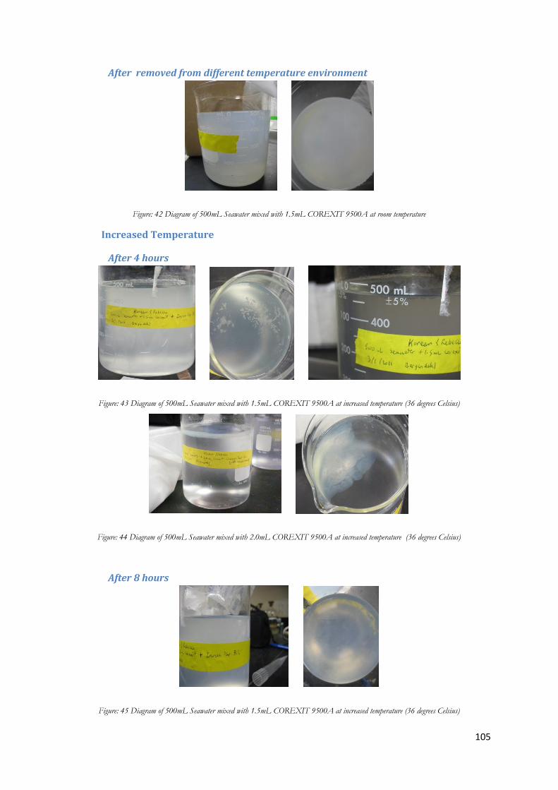
105
After removed from different temperature environment
Figure: 42 Diagram of 500mL Seawater mixed with 1.5mL COREXIT 9500A at room temperature
Increased Temperature
After 4 hours
Figure: 43 Diagram of 500mL Seawater mixed with 1.5mL COREXIT 9500A at increased temperature (36 degrees Celsius)
Figure: 44 Diagram of 500mL Seawater mixed with 2.0mL COREXIT 9500A at increased temperature (36 degrees Celsius)
After 8 hours
Figure: 45 Diagram of 500mL Seawater mixed with 1.5mL COREXIT 9500A at increased temperature (36 degrees Celsius)
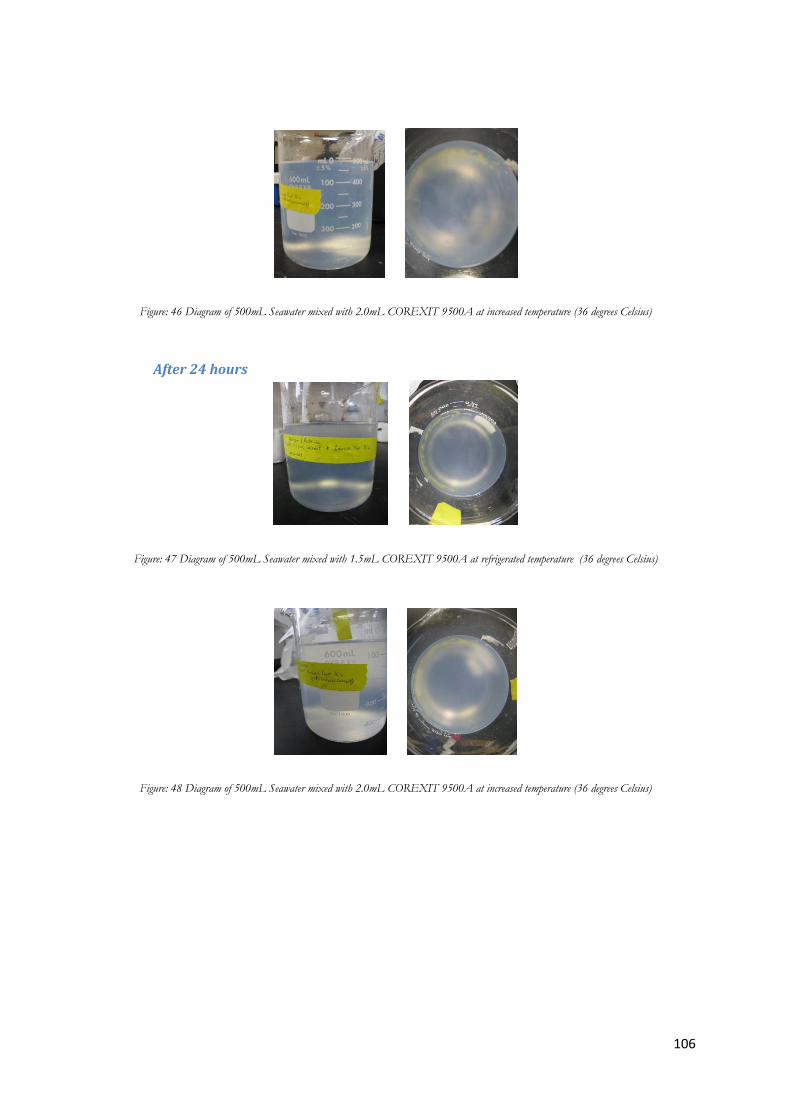
106
Figure: 46 Diagram of 500mL Seawater mixed with 2.0mL COREXIT 9500A at increased temperature (36 degrees Celsius)
After 24 hours
Figure: 47 Diagram of 500mL Seawater mixed with 1.5mL COREXIT 9500A at refrigerated temperature (36 degrees Celsius)
Figure: 48 Diagram of 500mL Seawater mixed with 2.0mL COREXIT 9500A at increased temperature (36 degrees Celsius)
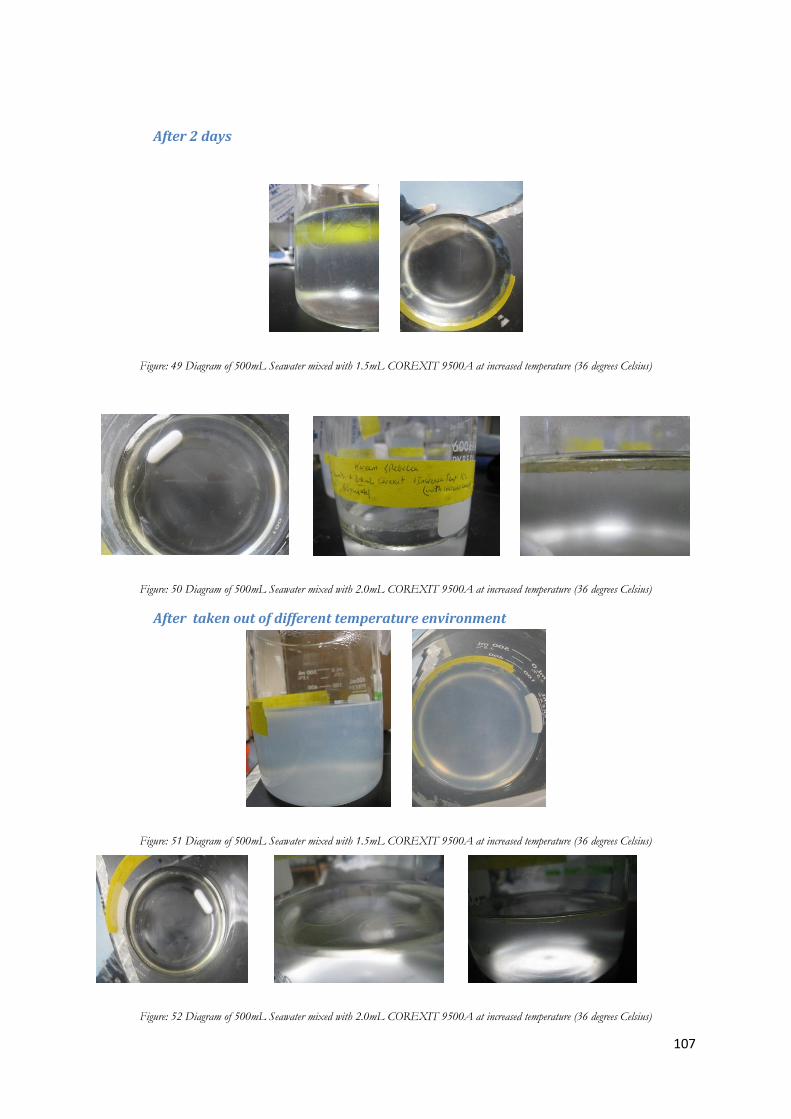
107
After 2 days
Figure: 49 Diagram of 500mL Seawater mixed with 1.5mL COREXIT 9500A at increased temperature (36 degrees Celsius)
Figure: 50 Diagram of 500mL Seawater mixed with 2.0mL COREXIT 9500A at increased temperature (36 degrees Celsius)
After taken out of different temperature environment
Figure: 51 Diagram of 500mL Seawater mixed with 1.5mL COREXIT 9500A at increased temperature (36 degrees Celsius)
Figure: 52 Diagram of 500mL Seawater mixed with 2.0mL COREXIT 9500A at increased temperature (36 degrees Celsius)
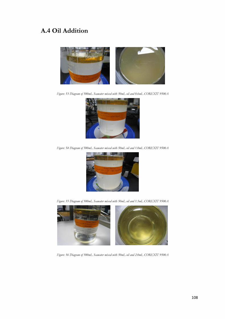
108
A.4 Oil Addition
Figure: 53 Diagram of 500mL Seawater mixed with 50mL oil and 0.6mL COREXIT 9500A
Figure: 54 Diagram of 500mL Seawater mixed with 50mL oil and 1.0mL COREXIT 9500A
Figure: 55 Diagram of 500mL Seawater mixed with 50mL oil and 1.5mL COREXIT 9500A
Figure: 56 Diagram of 500mL Seawater mixed with 50mL oil and 2.0mL COREXIT 9500A
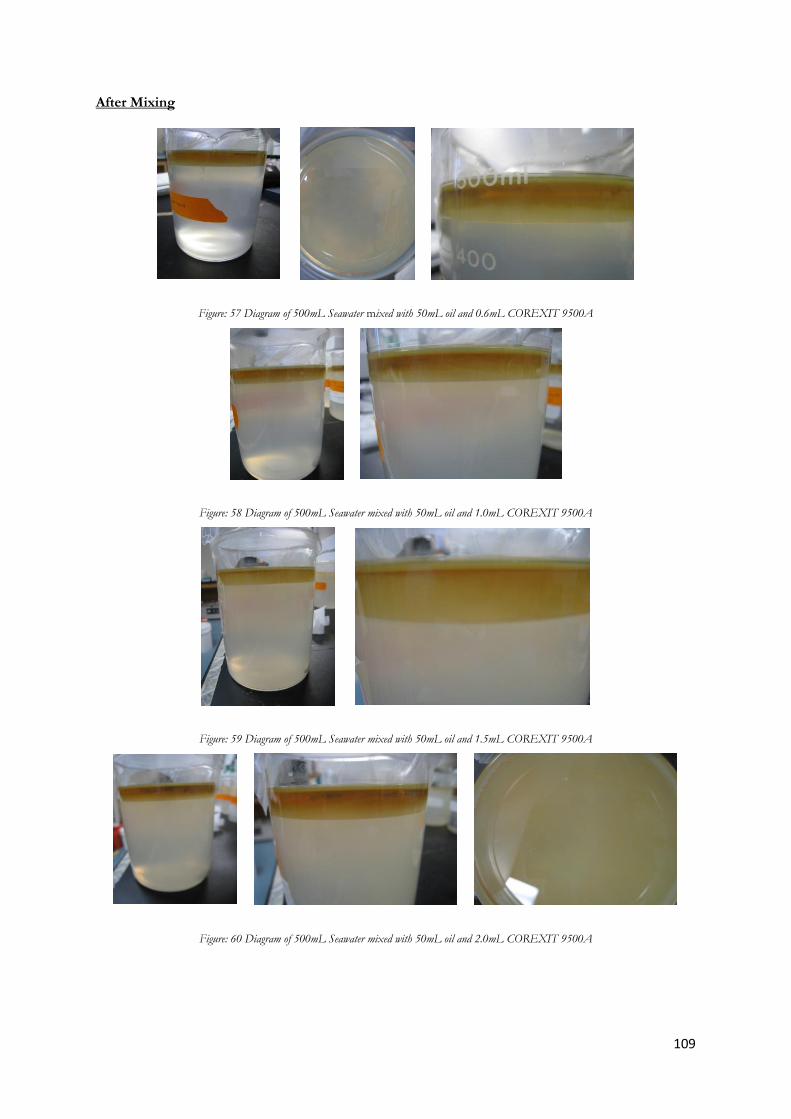
109
After Mixing
Figure: 57 Diagram of 500mL Seawater mixed with 50mL oil and 0.6mL COREXIT 9500A
Figure: 58 Diagram of 500mL Seawater mixed with 50mL oil and 1.0mL COREXIT 9500A
Figure: 59 Diagram of 500mL Seawater mixed with 50mL oil and 1.5mL COREXIT 9500A
Figure: 60 Diagram of 500mL Seawater mixed with 50mL oil and 2.0mL COREXIT 9500A
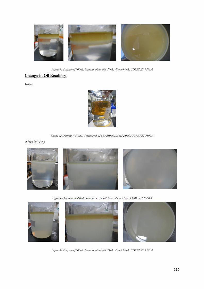
110
Figure: 61 Diagram of 500mL Seawater mixed with 50mL oil and 4.0mL COREXIT 9500A
Change in Oil Readings
Initial
Figure: 62 Diagram of 500mL Seawater mixed with 250mL oil and 2.0mL COREXIT 9500A
After Mixing
Figure: 63 Diagram of 500mL Seawater mixed with 5mL oil and 2.0mL COREXIT 9500A
Figure: 64 Diagram of 500mL Seawater mixed with 25mL oil and 2.0mL COREXIT 9500A
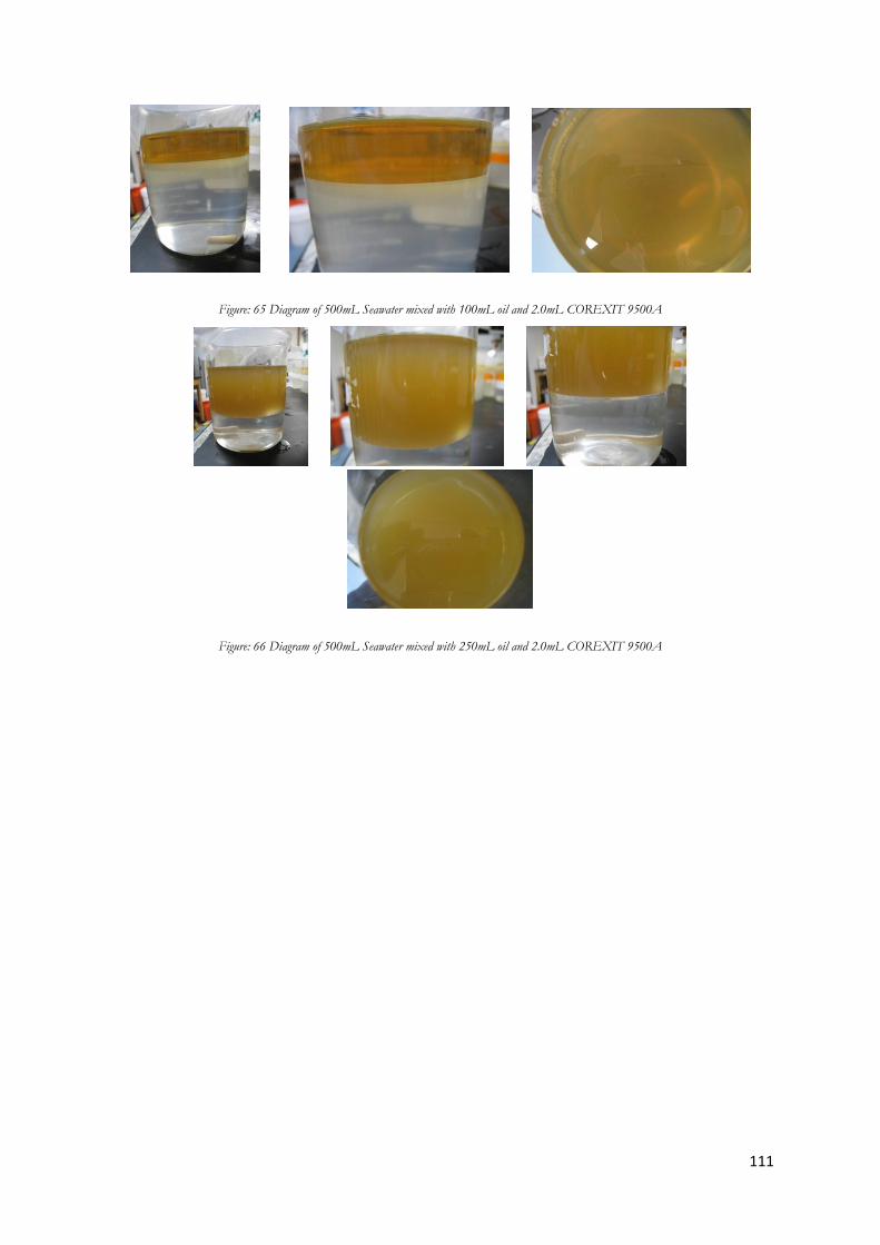
111
Figure: 65 Diagram of 500mL Seawater mixed with 100mL oil and 2.0mL COREXIT 9500A
Figure: 66 Diagram of 500mL Seawater mixed with 250mL oil and 2.0mL COREXIT 9500A
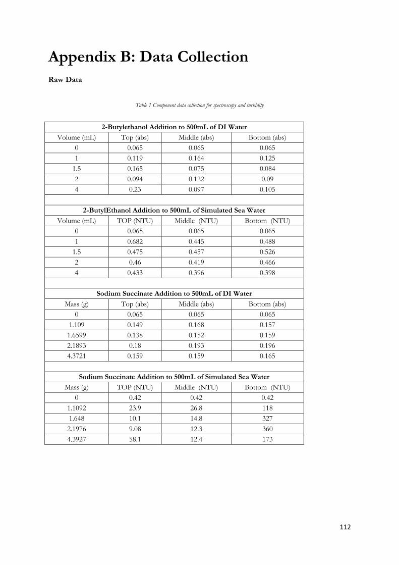
112
Appendix B: Data Collection Raw Data
Table 1 Component data collection for spectroscopy and turbidity
2-Butylethanol Addition to 500mL of DI Water
Volume (mL) Top (abs) Middle (abs) Bottom (abs)
0 0.065 0.065 0.065
1 0.119 0.164 0.125
1.5 0.165 0.075 0.084
2 0.094 0.122 0.09
4 0.23 0.097 0.105
2-ButylEthanol Addition to 500mL of Simulated Sea Water
Volume (mL) TOP (NTU) Middle (NTU) Bottom (NTU)
0 0.065 0.065 0.065
1 0.682 0.445 0.488
1.5 0.475 0.457 0.526
2 0.46 0.419 0.466
4 0.433 0.396 0.398
Sodium Succinate Addition to 500mL of DI Water
Mass (g) Top (abs) Middle (abs) Bottom (abs)
0 0.065 0.065 0.065
1.109 0.149 0.168 0.157
1.6599 0.138 0.152 0.159
2.1893 0.18 0.193 0.196
4.3721 0.159 0.159 0.165
Sodium Succinate Addition to 500mL of Simulated Sea Water
Mass (g) TOP (NTU) Middle (NTU) Bottom (NTU)
0 0.42 0.42 0.42
1.1092 23.9 26.8 118
1.648 10.1 14.8 327
2.1976 9.08 12.3 360
4.3927 58.1 12.4 173
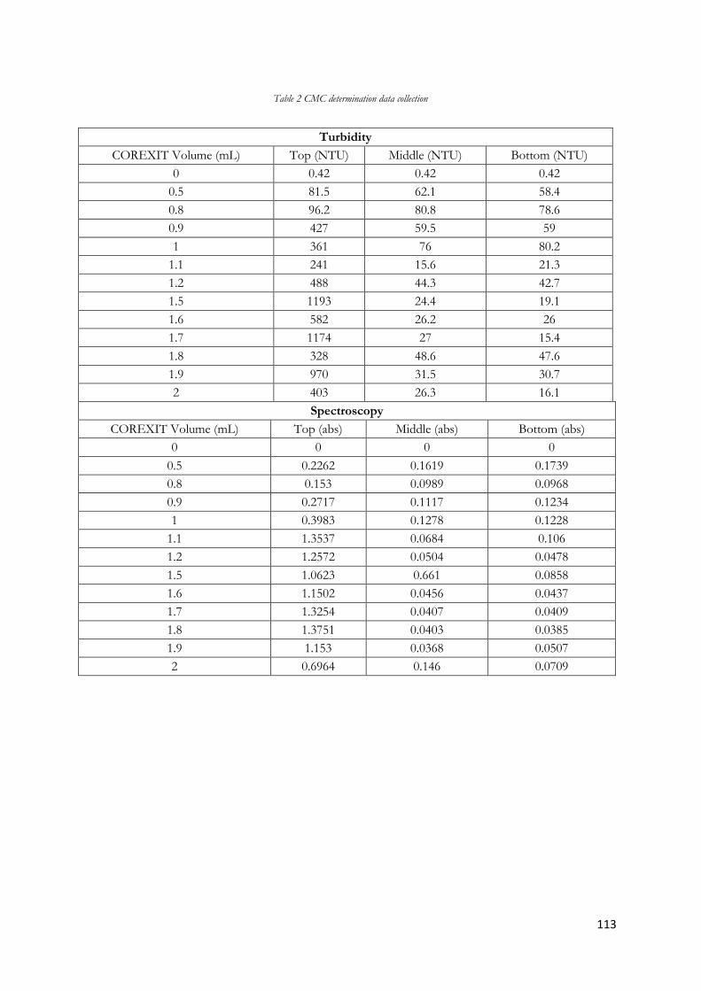
113
Table 2 CMC determination data collection
Turbidity
COREXIT Volume (mL) Top (NTU) Middle (NTU) Bottom (NTU)
0 0.42 0.42 0.42
0.5 81.5 62.1 58.4
0.8 96.2 80.8 78.6
0.9 427 59.5 59
1 361 76 80.2
1.1 241 15.6 21.3
1.2 488 44.3 42.7
1.5 1193 24.4 19.1
1.6 582 26.2 26
1.7 1174 27 15.4
1.8 328 48.6 47.6
1.9 970 31.5 30.7
2 403 26.3 16.1
Spectroscopy
COREXIT Volume (mL) Top (abs) Middle (abs) Bottom (abs)
0 0 0 0
0.5 0.2262 0.1619 0.1739
0.8 0.153 0.0989 0.0968
0.9 0.2717 0.1117 0.1234
1 0.3983 0.1278 0.1228
1.1 1.3537 0.0684 0.106
1.2 1.2572 0.0504 0.0478
1.5 1.0623 0.661 0.0858
1.6 1.1502 0.0456 0.0437
1.7 1.3254 0.0407 0.0409
1.8 1.3751 0.0403 0.0385
1.9 1.153 0.0368 0.0507
2 0.6964 0.146 0.0709
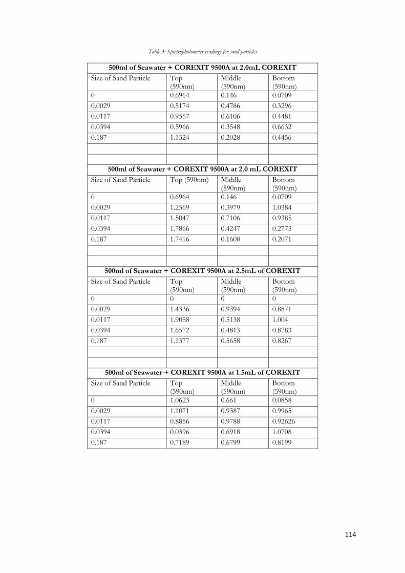
114
Table 3: Spectrophotometer readings for sand particles
500ml of Seawater + COREXIT 9500A at 2.0mL COREXIT
Size of Sand Particle Top (590nm)
Middle (590nm)
Bottom (590nm)
0 0.6964 0.146 0.0709
0.0029 0.5174 0.4786 0.3296
0.0117 0.9557 0.6106 0.4481
0.0394 0.5966 0.3548 0.6632
0.187 1.1324 0.2028 0.4456
500ml of Seawater + COREXIT 9500A at 2.0 mL COREXIT
Size of Sand Particle Top (590nm) Middle (590nm)
Bottom (590nm)
0 0.6964 0.146 0.0709
0.0029 1.2569 0.3979 1.0384
0.0117 1.5047 0.7106 0.9385
0.0394 1.7866 0.4247 0.2773
0.187 1.7416 0.1608 0.2071
500ml of Seawater + COREXIT 9500A at 2.5mL of COREXIT
Size of Sand Particle Top (590nm)
Middle (590nm)
Bottom (590nm)
0 0 0 0
0.0029 1.4336 0.9394 0.8871
0.0117 1.9058 0.5138 1.004
0.0394 1.6572 0.4813 0.8783
0.187 1.1377 0.5658 0.8267
500ml of Seawater + COREXIT 9500A at 1.5mL of COREXIT
Size of Sand Particle Top (590nm)
Middle (590nm)
Bottom (590nm)
0 1.0623 0.661 0.0858
0.0029 1.1071 0.9387 0.9965
0.0117 0.8856 0.9788 0.92626
0.0394 0.0396 0.6918 1.0708
0.187 0.7189 0.6799 0.8199
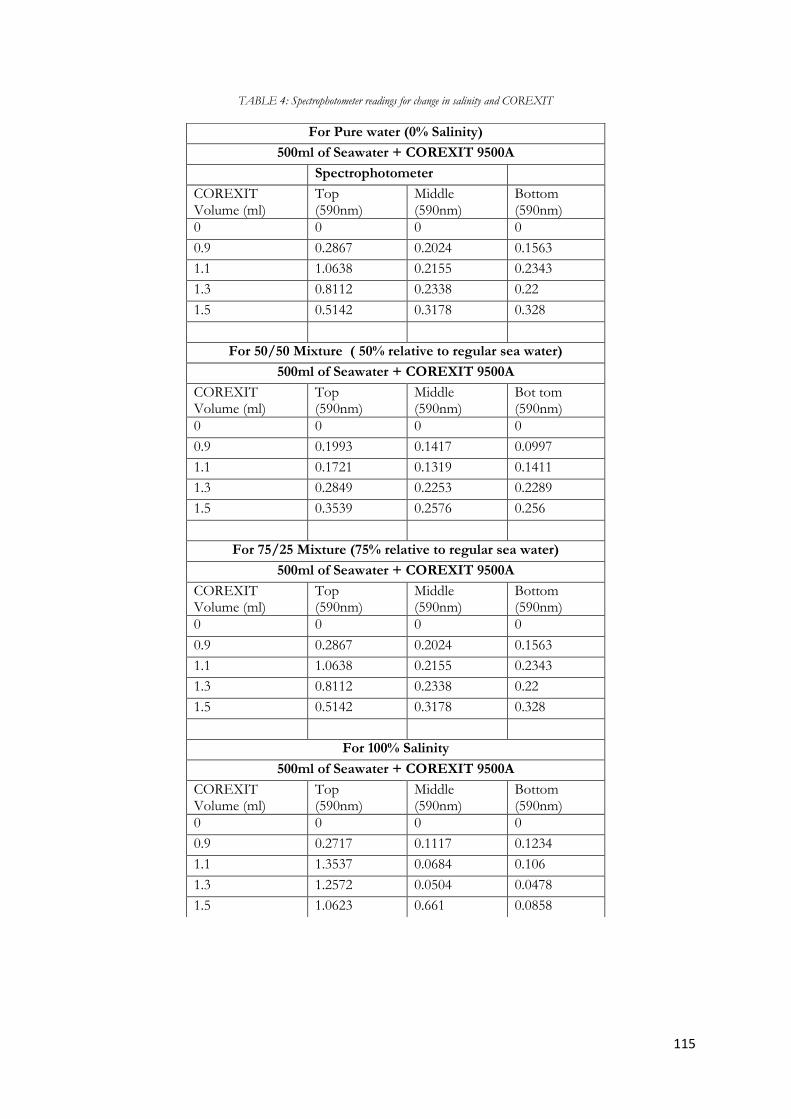
115
TABLE 4: Spectrophotometer readings for change in salinity and COREXIT
For Pure water (0% Salinity)
500ml of Seawater + COREXIT 9500A
Spectrophotometer
COREXIT Volume (ml)
Top (590nm)
Middle (590nm)
Bottom (590nm)
0 0 0 0
0.9 0.2867 0.2024 0.1563
1.1 1.0638 0.2155 0.2343
1.3 0.8112 0.2338 0.22
1.5 0.5142 0.3178 0.328
For 50/50 Mixture ( 50% relative to regular sea water)
500ml of Seawater + COREXIT 9500A
COREXIT Volume (ml)
Top (590nm)
Middle (590nm)
Bot tom (590nm)
0 0 0 0
0.9 0.1993 0.1417 0.0997
1.1 0.1721 0.1319 0.1411
1.3 0.2849 0.2253 0.2289
1.5 0.3539 0.2576 0.256
For 75/25 Mixture (75% relative to regular sea water)
500ml of Seawater + COREXIT 9500A
COREXIT Volume (ml)
Top (590nm)
Middle (590nm)
Bottom (590nm)
0 0 0 0
0.9 0.2867 0.2024 0.1563
1.1 1.0638 0.2155 0.2343
1.3 0.8112 0.2338 0.22
1.5 0.5142 0.3178 0.328
For 100% Salinity
500ml of Seawater + COREXIT 9500A
COREXIT Volume (ml)
Top (590nm)
Middle (590nm)
Bottom (590nm)
0 0 0 0
0.9 0.2717 0.1117 0.1234
1.1 1.3537 0.0684 0.106
1.3 1.2572 0.0504 0.0478
1.5 1.0623 0.661 0.0858
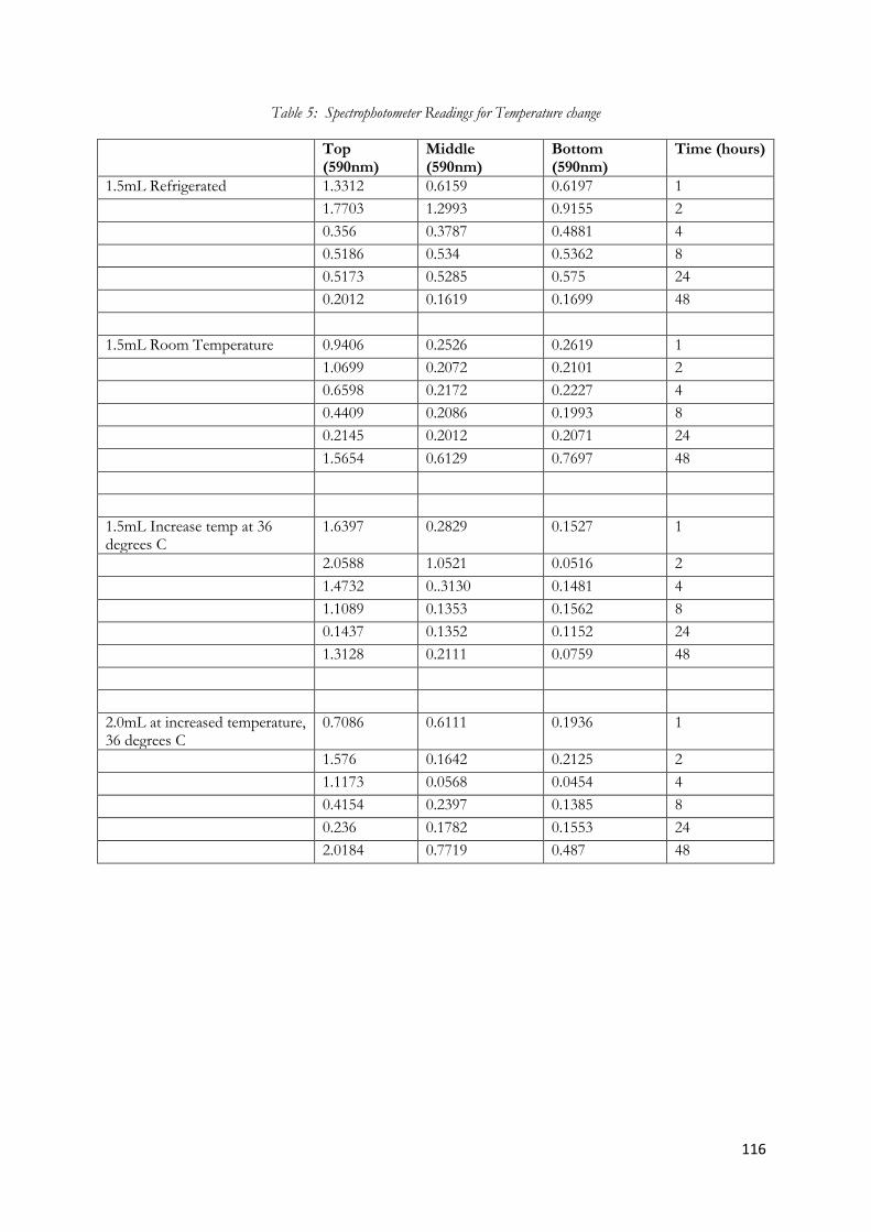
116
Table 5: Spectrophotometer Readings for Temperature change
Top (590nm)
Middle (590nm)
Bottom (590nm)
Time (hours)
1.5mL Refrigerated 1.3312 0.6159 0.6197 1
1.7703 1.2993 0.9155 2
0.356 0.3787 0.4881 4
0.5186 0.534 0.5362 8
0.5173 0.5285 0.575 24
0.2012 0.1619 0.1699 48
1.5mL Room Temperature 0.9406 0.2526 0.2619 1
1.0699 0.2072 0.2101 2
0.6598 0.2172 0.2227 4
0.4409 0.2086 0.1993 8
0.2145 0.2012 0.2071 24
1.5654 0.6129 0.7697 48
1.5mL Increase temp at 36 degrees C
1.6397 0.2829 0.1527 1
2.0588 1.0521 0.0516 2
1.4732 0..3130 0.1481 4
1.1089 0.1353 0.1562 8
0.1437 0.1352 0.1152 24
1.3128 0.2111 0.0759 48
2.0mL at increased temperature, 36 degrees C
0.7086 0.6111 0.1936 1
1.576 0.1642 0.2125 2
1.1173 0.0568 0.0454 4
0.4154 0.2397 0.1385 8
0.236 0.1782 0.1553 24
2.0184 0.7719 0.487 48
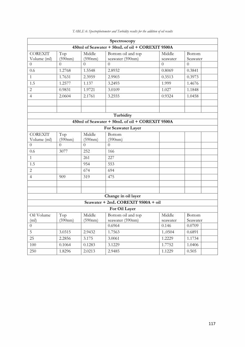
117
TABLE 6: Spectrophotometer and Turbidity results for the addition of oil results
Spectroscopy
450ml of Seawater + 50mL of oil + COREXIT 9500A
COREXIT Volume (ml)
Top (590nm)
Middle (590nm)
Bottom oil and top seawater (590nm)
Middle seawater
Bottom Seawater
0 0 0 0 0 0
0.6 1.2768 1.5548 2.8932 0.8069 0.3841
1 1.7631 2.3959 2.9903 0.3513 0.3973
1.5 1.2577 1.137 3.2493 1.999 1.4676
2 0.9831 1.9721 3.0109 1.027 1.1848
4 2.0604 2.1761 3.2555 0.9324 1.0458
Turbidity
450ml of Seawater + 50mL of oil + COREXIT 9500A
For Seawater Layer
COREXIT Volume (ml)
Top (590nm)
Middle (590nm)
Bottom (590nm)
0 0 0 0
0.6 3077 252 166
1 261 227
1.5 954 553
2 674 694
4 909 319 475
Change in oil layer
Seawater + 2mL COREXIT 9500A + oil
For Oil Layer
Oil Volume (ml)
Top (590nm)
Middle (590nm)
Bottom oil and top seawater (590nm)
Middle seawater
Bottom Seawater
0 0.6964 0.146 0.0709
5 3.0315 2.9432 1.7563 1..0504 0.6891
25 2.2856 3.175 3.0061 1.2229 1.1734
100 0.1064 0.1283 3.1229 1.7752 1.0406
250 1.8296 2.0213 2.9485 1.1229 0.505
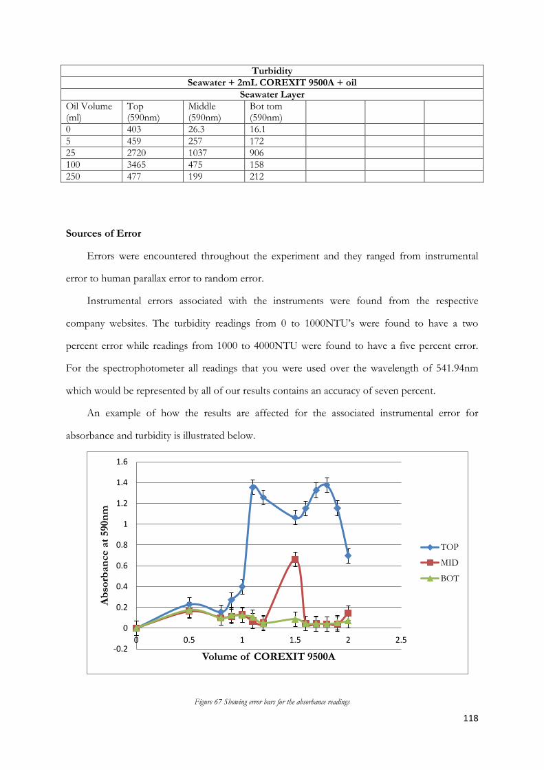
118
Turbidity
Seawater + 2mL COREXIT 9500A + oil
Seawater Layer
Oil Volume (ml)
Top (590nm)
Middle (590nm)
Bot tom (590nm)
0 403 26.3 16.1
5 459 257 172
25 2720 1037 906
100 3465 475 158
250 477 199 212
Sources of Error
Errors were encountered throughout the experiment and they ranged from instrumental
error to human parallax error to random error.
Instrumental errors associated with the instruments were found from the respective
company websites. The turbidity readings from 0 to 1000NTU’s were found to have a two
percent error while readings from 1000 to 4000NTU were found to have a five percent error.
For the spectrophotometer all readings that you were used over the wavelength of 541.94nm
which would be represented by all of our results contains an accuracy of seven percent.
An example of how the results are affected for the associated instrumental error for
absorbance and turbidity is illustrated below.
Figure 67 Showing error bars for the absorbance readings
-0.2
0
0.2
0.4
0.6
0.8
1
1.2
1.4
1.6
0 0.5 1 1.5 2 2.5
Ab
sorb
an
ce a
t 590n
m
Volume of COREXIT 9500A
TOP
MID
BOT
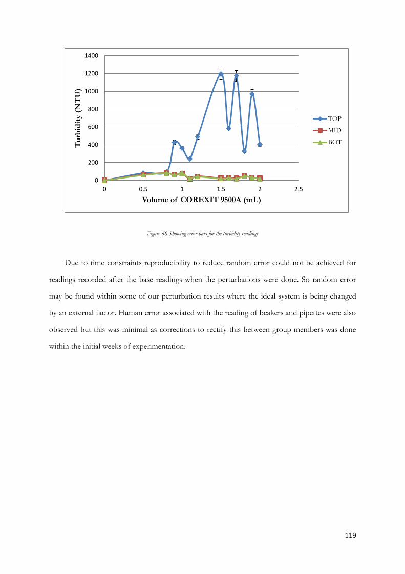
119
Figure 68 Showing error bars for the turbidity readings
Due to time constraints reproducibility to reduce random error could not be achieved for
readings recorded after the base readings when the perturbations were done. So random error
may be found within some of our perturbation results where the ideal system is being changed
by an external factor. Human error associated with the reading of beakers and pipettes were also
observed but this was minimal as corrections to rectify this between group members was done
within the initial weeks of experimentation.
0
200
400
600
800
1000
1200
1400
0 0.5 1 1.5 2 2.5
Tu
rbid
ity (
NT
U)
Volume of COREXIT 9500A (mL)
TOP
MID
BOT
![Controlled polymers for pigment dispersants€¦ · pigment dispersants [6]. In this contribution acrylic block copolymer type "controlled pigment dispersants" are presented based](https://static.fdocuments.us/doc/165x107/5ea9e9ef0447ea48144fa6b6/controlled-polymers-for-pigment-pigment-dispersants-6-in-this-contribution-acrylic.jpg)