Disentangling a Deep Learned Volume Formula

Jessica Cravena , Vishnu Jejjalaa , Arjun Karb

aMandelstam Institute for Theoretical Physics, School of Physics, NITheP, and CoE-MaSS,

University of the Witwatersrand, Johannesburg, WITS 2050, South AfricabDepartment of Physics and Astronomy, University of British Columbia,

6224 Agricultural Road, Vancouver, BC V6T 1Z1, Canada

E-mail: jessica.craven1@students.wits.ac.za,

vishnu@neo.phys.wits.ac.za, arjunkar@phas.ubc.ca

Abstract: We present a simple phenomenological formula which approximates the hyper-

bolic volume of a knot using only a single evaluation of its Jones polynomial at a root of

unity. The average error is just 2.86% on the first 1.7 million knots, which represents a large

improvement over previous formulas of this kind. To find the approximation formula, we

use layer-wise relevance propagation to reverse engineer a black box neural network which

achieves a similar average error for the same approximation task when trained on 10% of the

total dataset. The particular roots of unity which appear in our analysis cannot be written as

e2πi/(k+2) with integer k; therefore, the relevant Jones polynomial evaluations are not given

by unknot-normalized expectation values of Wilson loop operators in conventional SU(2)

Chern–Simons theory with level k. Instead, they correspond to an analytic continuation of

such expectation values to fractional level. We briefly review the continuation procedure and

comment on the presence of certain Lefschetz thimbles, to which our approximation formula

is sensitive, in the analytically continued Chern–Simons integration cycle.

arX

iv:2

012.

0395

5v2

[he

p-th

] 7

Jun

202

1

Contents

1 Introduction 2

2 Chern–Simons theory 5

2.1 Knot invariants 5

2.2 Analytic continuation 8

3 Machine learning 11

3.1 Neural networks 12

3.2 Layer-wise relevance propagation 13

3.3 Strategies for analyzing the network 14

4 An approximation formula for the hyperbolic volume 15

4.1 Interpretable deep learning 15

4.2 Implications in Chern–Simons theory 21

5 Discussion 24

A Basic neural network setup 27

B Khovanov homology, Jones coefficients, and volume 29

B.1 Khovanov homology 29

B.2 Power law behavior of coefficients 30

C Normalizations, orientation, and framing 31

D t-distributed stochastic neighbor embedding of knot invariants 35

D.1 t-distributed stochastic neighbor embedding 35

D.2 Volume and Chern–Simons invariant 36

E Other experiments 37

E.1 The HOMFLY-PT and Khovanov polynomials 38

E.2 Representations of J2(K; q) 38

E.3 Small networks 40

E.4 Symbolic regression 41

– 1 –

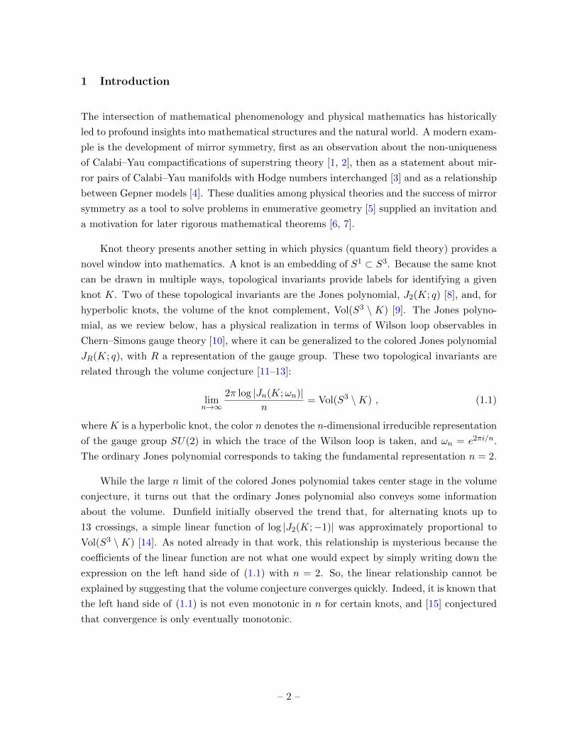
1 Introduction

The intersection of mathematical phenomenology and physical mathematics has historically

led to profound insights into mathematical structures and the natural world. A modern exam-

ple is the development of mirror symmetry, first as an observation about the non-uniqueness

of Calabi–Yau compactifications of superstring theory [1, 2], then as a statement about mir-

ror pairs of Calabi–Yau manifolds with Hodge numbers interchanged [3] and as a relationship

between Gepner models [4]. These dualities among physical theories and the success of mirror

symmetry as a tool to solve problems in enumerative geometry [5] supplied an invitation and

a motivation for later rigorous mathematical theorems [6, 7].

Knot theory presents another setting in which physics (quantum field theory) provides a

novel window into mathematics. A knot is an embedding of S1 ⊂ S3. Because the same knot

can be drawn in multiple ways, topological invariants provide labels for identifying a given

knot K. Two of these topological invariants are the Jones polynomial, J2(K; q) [8], and, for

hyperbolic knots, the volume of the knot complement, Vol(S3 \ K) [9]. The Jones polyno-

mial, as we review below, has a physical realization in terms of Wilson loop observables in

Chern–Simons gauge theory [10], where it can be generalized to the colored Jones polynomial

JR(K; q), with R a representation of the gauge group. These two topological invariants are

related through the volume conjecture [11–13]:

limn→∞

2π log |Jn(K;ωn)|n

= Vol(S3 \K) , (1.1)

where K is a hyperbolic knot, the color n denotes the n-dimensional irreducible representation

of the gauge group SU(2) in which the trace of the Wilson loop is taken, and ωn = e2πi/n.

The ordinary Jones polynomial corresponds to taking the fundamental representation n = 2.

While the large n limit of the colored Jones polynomial takes center stage in the volume

conjecture, it turns out that the ordinary Jones polynomial also conveys some information

about the volume. Dunfield initially observed the trend that, for alternating knots up to

13 crossings, a simple linear function of log |J2(K;−1)| was approximately proportional to

Vol(S3 \K) [14]. As noted already in that work, this relationship is mysterious because the

coefficients of the linear function are not what one would expect by simply writing down the

expression on the left hand side of (1.1) with n = 2. So, the linear relationship cannot be

explained by suggesting that the volume conjecture converges quickly. Indeed, it is known that

the left hand side of (1.1) is not even monotonic in n for certain knots, and [15] conjectured

that convergence is only eventually monotonic.

– 2 –

Subsequently, a neural network predicted the hyperbolic volume from the Jones poly-

nomial with 97.55 ± 0.10% accuracy for all hyperbolic knots up to 15 crossings using only

10% of the dataset of 313, 209 knots for training [16]. The input to the network was a vector

consisting of the maximum and minimum degrees of the Jones polynomial along with its

integer coefficients. The network’s accuracy is essentially optimal for the following reason:

knots with different hyperbolic volumes can have the same Jones polynomial, and when this

happens, the volumes typically differ by about 3%. This represented a large improvement

over the approximation formula using J2(K;−1), but introduced many more free parameters

(the weights and biases of the neural network) and completely obscured the true functional

dependence on J2(K; q).

This work in experimental mathematics established that there is more information about

the volume contained in the full Jones polynomial than in the single evaluation J2(K;−1).1

Indeed, training on only 319 knots (0.1% of the dataset) is sufficient to extract this additional

information. Moreover, the predictions apply to all hyperbolic knots, not just the alternating

ones. The neural network, however, is a black box that learns semantics without knowing

any syntax. While machine learning successfully identifies relationships between topological

invariants of hyperbolic knots, we do not have an analytic understanding of why this occurs or

how the machine learns the relationship in the first place. The aim of this paper is to determine

which aspects of the input are most important for the neural network’s considerations and

to use this to deduce a simpler functional relationship between the Jones polynomial and

the hyperbolic volume that depends on only an O(1) number of free parameters. In other

words, we seek an approximation formula which similarly outperforms the formula based on

J2(K;−1), but which does not rely on the complicated structure of a neural network.

The main result obtained in this work is an approximation formula for the hyperbolic

volume of a knot in terms of a single evaluation of its Jones polynomial.

V3/4(K) = 6.20 log (|J2(K; e3πi/4)|+ 6.77)− 0.94 . (1.2)

This formula is numerical in nature, and we have no sharp error bounds, but it achieves

an accuracy of more than 97% on the first 1.7 million hyperbolic knots. The phase e3πi/4

can be adjusted to some degree to obtain similar formulas which perform almost as well;

we explore these alternatives. We obtain (1.2) and its analogues by reverse engineering the

behavior of the aforementioned neural network, a task which is generally considered difficult

in the machine learning community. In our case, it is possible due to the simplicity of the

1We refer loosely to the information contained in certain invariants, as all of our results are numerical and

therefore “probably approximately correct” [17].

– 3 –

underlying neural network architecture and the power of layer-wise relevance propagation, a

network analysis technique which we review.

Since the phase e3πi/4 cannot be written as e2πi/(k+2) for integer k, (1.2) suggests that we

should consider analytically continued Chern–Simons theory, which was previously explored

as a possible route to understand the volume conjecture [18]. Specifically, the evaluations of

the Jones polynomial that are relevant for us correspond to fractional Chern–Simons levels

k = 23 and k = 1

2 , which must be understood in the context of the analytically continued

theory due to the integer level restriction normally enforced by gauge invariance. We provide

a review of the main points of the analytically continued theory, as our results have some

speculative bearing on which Lefschetz thimbles should contribute to the path integral at

various values of n and k. Our interpretations pass several sanity checks when compared with

the main lessons of [18], and we use our results to formulate an alternative version of the

volume conjecture.

Though we do not have a complete explanation for why (1.2) predicts the volume so well,

its implications are intriguing. It points to the existence of a sort of quantum/semiclassical

duality between SU(2) and SL(2,C) Chern–Simons theory, since some simple numerical co-

efficients are enough to transform a strong coupling object (the Jones polynomial at small k)

into a weak coupling one (the hyperbolic volume). This is reminiscent of the shift k → k + 2

induced by the one-loop correction in the SU(2) Chern–Simons path integral [10], which trans-

forms a semiclassical approximation into a more quantum result via a single O(1) parameter.

We can explore this phenomenon in a preliminary way by checking whether J2 contains any

information about Jn for n > 2 and some O(1) phases like the ones appearing in the volume

conjecture. Computing 11, 921 colored Jones polynomials in the adjoint representation of

SU(2), we notice from Figure 1 that

|J3(K;ω3)| ∼ J2(K;ω2)2 . (1.3)

Comparing to the volume conjecture (1.1), this suggests that the ordinary Jones polynomial

has some knowledge of the behavior of higher colors and in particular the n→∞ limit.2

The organization of this paper is as follows. In Section 2, we review relevant aspects

of Chern–Simons theory, including its relationship to knot invariants and its analytic con-

tinuation. In Section 3, we describe the machine learning methods we employ, particularly

neural networks and layer-wise relevance propagation. In Section 4, we analyze the struc-

ture of the neural network and, using layer-wise relevance propagation, deduce a relationship

between evaluations of the Jones polynomial of a hyperbolic knot and the volume of its

2This analysis was performed in collaboration with Onkar Parrikar.

– 4 –

-600 -400 -200 200 400 600

5000

10000

15000

20000

Figure 1: The n = 2 and n = 3 colored Jones polynomials evaluated at roots of unity show

a quadratic relation.

knot complement. We also comment on the implications of our numerics for the presence

of certain integration cycles in the analytically continued Chern–Simons path integral as a

function of coupling. In Section 5, we discuss the results we obtain and propose some future

directions. We also provide several appendices which outline details about the implemen-

tation of our machine learning algorithms (Appendix A), results relating the scaling of the

Jones polynomial coefficients with the hyperbolic volume (Appendix B), details concerning

the various normalizations of the Jones polynomial in the mathematics and physics litera-

ture (Appendix C), a data analysis of knot invariants using t-distributed stochastic neighbor

embedding (Appendix D), and finally, an overview of related experiments (Appendix E).

2 Chern–Simons theory

We review several aspects of Chern–Simons theory, its relation to the colored Jones poly-

nomials and hyperbolic volumes of knots, and its analytic continuation away from integer

level.

2.1 Knot invariants

Chern–Simons theory is a three-dimensional topological quantum field theory which provides

a unifying language for the knot invariants with which we will be concerned [10, 13]. The

Chern–Simons function is defined, using a connection (or gauge field) A on an SU(2)-bundle

– 5 –

E over a three manifold M , as

W (A) =1

4π

∫M

Tr

[A ∧ dA+

2

3A ∧A ∧A

]. (2.1)

The trace is taken in the fundamental representation. The path integral of Chern–Simons

gauge theory is then given in the compact case by

Z(M) =

∫U

[DA] exp(ikW (A)) , (2.2)

where U is the space of SU(2) gauge fields modulo gauge transformations. The coupling k

is integer-quantized, k ∈ Z, to ensure gauge invariance. For SU(2) Chern–Simons theory on

M = S3, it was shown in [10] that the expectation value of a Wilson loop operator along the

knot, defined by

UR(K) = TrR P exp

(−∮KA

), (2.3)

is related to the colored Jones polynomials JR(K; q) of a knot K ⊂ S3 evaluated at q =

e2πi/(k+2). In our work, we will be interested in evaluations of the Jones polynomial (where

the representation R is the fundamental one) away from this particular root of unity, and

indeed away from all roots expressible as e2πi/(k+2) for some k ∈ Z. Strictly speaking, these

evaluations of the Jones polynomial are not provided by the usual formulation using the path

integral of Chern–Simons theory. However, evaluation at arbitrary phases e2πi/(k+2) for k ∈ Rcan be achieved by making use of the analytic continuation machinery developed in [18].

We will also be interested in a complex-valued Chern–Simons function W (A) obtained

from an SL(2,C)-bundle EC over M with connection A. In the non-compact SL(2,C) case,

there are two couplings, and the path integral is

Z(M) =

∫UC

[DA][DA] exp

[it

2W (A) +

it

2W (A)

], (2.4)

where UC is the space of SL(2,C) gauge fields modulo gauge transformations, and the complex

couplings t = ` + is and t = ` − is obey s ∈ C and ` ∈ Z. The coupling `, which multiplies

the real part Re(W ), is integer-quantized for the same reason as k was in the compact case.

On the other hand, Im(W ) is a well-defined complex number even under arbitrary gauge

transformations, so s can (in principle) take any complex value.3 There is a particularly

interesting saddle point (flat connection) which contributes to Z(M) in the case where M

admits a complete hyperbolic metric. Such manifolds are relevant for us because, as explained

by Thurston [19], most knots K admit a complete hyperbolic metric on their complements

3Usually one takes s ∈ R to ensure that the argument of the path integral is bounded, but via analytic

continuation one can obtain something sensible for more general s [18].

– 6 –

S3 \K. The knot complement S3 \K is the three manifold obtained by drilling out a tubular

neighborhood around the knot K ⊂ S3. This complement is topologically distinct from S3,

and the knot shrinks to a torus cusp in the complete hyperbolic metric.4 For such hyperbolic

M , there exists a “geometric” flat SL(2,C) connection A−5 for which Im(W (A−)) is related

to the volume of the hyperbolic metric on M via Im(W (A−)) = Vol(M)/2π.6 Thus, SL(2,C)

Chern–Simons theory is intimately related to the hyperbolic volumes of three manifolds, as

this quantity makes a saddle point contribution to the path integral.

One of the primary motivations for both this work and the work of [18] was the so-

called volume conjecture [11], which relates the colored Jones invariants and the hyperbolic

volume of three manifolds (which, by the Mostow–Prasad rigidity theorem, is a topological

invariant of any hyperbolic M). As written in the introduction and reproduced here, the

volume conjecture states [11–13]

limn→∞

2π log |Jn(K; e2πi/n)|n

= Vol(S3 \K) , (2.5)

where n is the n-dimensional irreducible representation of SU(2). Thus, the natural unifying

language for the volume conjecture is SU(2) and SL(2,C) Chern–Simons theory, because the

knot invariants appearing on both the left and right hand sides are quantities which appear

in the calculation of the Chern–Simons path integral.7

In writing the above relationship, we must be careful to specify precisely what we mean

by the colored Jones invariants Jn(K; q). We choose a normalization of the colored Jones

invariants so that they are Laurent polynomials in the variable q, and that the unknot 01

obeys Jn(01; q) = 1. As explained clearly in Section 2.5.3 of [18], this choice implies that the

colored Jones polynomials are reproduced by the ratio of two Chern–Simons path integrals.

The numerator of this ratio has a single Wilson loop insertion along the knot K ⊂ S3, and

the denominator has a Wilson loop along an unknot 01 ⊂ S3. Explicitly, we have

Jn(K; q = e2πi/(k+2)) =

∫U [DA] Un(K) exp(ikW (A))∫U [DA] Un(01) exp(ikW (A))

, (2.6)

and the manifold implicit in W (A) is M = S3. It is for this reason that the statement of

the volume conjecture only involves evaluation of the n-colored Jones polynomial at integer

4We emphasize that this complete hyperbolic metric on S3 \K does not descend somehow from a metric on

S3. It exists due to an ideal tetrahedral decomposition of S3 \K, where each tetrahedron has an embedding

in H3, and the embeddings can be glued together in a consistent way.5We choose this notation to match (5.61) of [18], and comment further in footnote 20.6The real part Re(W (A−)) of the geometric connection is proportional to a number which is often called

the “Chern–Simons invariant” of M .7This combination of invariants, the colored Jones polynomial and hyperbolic volume, was explored in the

context of entanglement entropy of Euclidean path integral states in [20, 21].

– 7 –

k = n − 2, whereas to understand the conjecture in Chern–Simons theory it is necessary to

analytically continue the path integral away from integer values of k. Without normalization,

the path integral yields an expression which vanishes at q = e2πi/n, and this vanishing is

removed by dividing by the unknot expectation. In short, we can either measure how fast

the path integral vanishes by computing a derivative with respect to k (which relies on the

analytic structure of the function), or we can explicitly divide by a function which vanishes

equally as fast to obtain a finite ratio.8

2.2 Analytic continuation

With these conventions in hand, we will provide a brief review of the main results in [18],

essentially to introduce the language, as we will make some speculative comments on the

relationship between our numerical results and the analytic techniques in [18]. To analytically

continue SU(2) Chern–Simons theory on S3\K away from integer values of k, [18] instructs us

to first rewrite the SU(2) path integral over A as an SL(2,C) path integral over A restricted

to a real integration cycle CR in the space of complex-valued connections modulo gauge

transformations UC. Analytic continuation occurs then by lifting CR to a cycle C in the

universal cover UC,9 where the Chern–Simons function W (A) is well-defined as a complex-

valued function. (Recall that large gauge transformations can modify the real part of W (A)

by a multiple of 2π.) In the presence of a Wilson loop along a knot, the relevant path integral

looks like ∫C⊂UC

[DA]

∫[Dρ] exp(I) , I = ikW (A) + iIn(ρ,A) . (2.7)

We have added an additional term that depends on a field ρ, which is associated with the

knot itself. The introduction of this field along with its action In is a way to absorb the

Wilson loop Un(K) into the exponential, and makes use of the Borel–Weil–Bott theorem. We

will not provide a discussion of this point, and simply refer interested readers to [18]; we will

only refer to the total exponential argument I from now on. We will just make one important

remark concerning In: when evaluated on a flat connection, In is proportional to n− 1 [18].

Therefore, up to an overall rescaling, I depends only on the combination

γ ≡ n− 1

k, (2.8)

8This subtle point, while discussed in this language in [22], is implicit throughout [18] (also see footnote 7

in [22], and note that our Jn(K; q) would be written as Jn(K; q)/Jn(01; q) in the notation of [22]).9This space can also be thought of as the space of complex-valued gauge fields modulo topologically trivial,

or “small,” gauge transformations.

– 8 –

when evaluated on a flat connection.10 If we wish to understand the volume conjecture, γ = 1

is held fixed in the semiclassical limit n, k →∞. When quoting values for γ, we have in mind

the ratio (2.6); in the bare path integral setup of [18], we would need to move slightly away

from γ = 1.11

The cycle C must be extended using the machinery of Morse theory; this extension

guarantees that the Ward identities will hold. Morse theory on UC, specifically with Re(I) as

a Morse function, plays a key role in this extension and in the definition of other integration

cycles. Analytic continuation away from a discrete set of points (integer values of k, in this

case) is not unique, and this corresponds to an ambiguity in lifting CR to C. The relatively

natural resolution in this situation is to ask that the path integral should have no exponentially

growing contributions as k →∞ with fixed n.12 This is equivalent to requiring that the colored

Jones polynomials, as defined in the mathematical literature, and the ratio of Chern–Simons

path integrals (2.6) should hold for more general q after replacing the path integrals with

their analytic continuations.13

Once the cycle C has been defined, we must vary the value of γ from zero to our desired

point. We begin at zero since we have defined a sort of boundary condition on C at k → ∞with fixed n by selecting the relatively natural analytic continuation just described. As we

vary γ, we must track the behavior of C. It may seem like there is nothing to keep track of,

but in fact there are subtle Stokes phenomena which must be taken into account, as we will

now briefly explain. The cycle C has a decomposition in terms of so-called Lefschetz thimbles

Jσ, which are cycles defined using Morse theory that each pass through precisely one critical

point σ of I, and are defined so that the path integral along them always converges:

C =∑σ

nσJσ . (2.9)

10This differs from the definition of γ in [18], where n/k was used instead. In that discussion, the semiclassical

limit was of much greater importance, and in that limit our definition becomes equal to n/k. However, as we

are working at n and k of O(1), we will keep the exact ratio implied by the value of I on a flat connection.11Actually, even with the ratio of path integrals, we need to move away from exactly γ = 1. We will continue

to write γ = 1 as the relevant point for the volume conjecture in the semiclassical limit, but the true value for

integer n and k is more like γ = n−1n−2

> 1.12As mentioned in [18], it is not quite clear how to enforce this condition on C for general knots, but we will

not need the details.13Conventions are not uniform across the mathematical literature, and the relevance of framing is often

unmentioned. See Appendix C for further discussion of the alignment between the path integral ratio (2.6)

and the mathematical definitions of J2.

– 9 –

These thimbles can intuitively be visualized as downward flow lines coming from a critical

point. Since our Morse function is Re(I), the path integral decreases exponentially when

following a downward flow line: it is for this reason that convergence is guaranteed.14

When crossing certain loci in the complex γ plane, known as Stokes lines, the decompo-

sition of C in terms of Lefschetz thimbles may be required to change in order to both preserve

the cycle C locally and ensure convergence of the path integral. Functionally, the coefficients

nσ change in exactly the right way to compensate for a similar jumping in the Lefschetz thim-

bles Jσ themselves. This jumping occurs for a cycle Jσ when there is a downward flow from

σ that ends at another critical point rather than flowing to −∞. Thus, recalling that critical

points σ of I on UC are flat SL(2,C) connections on S3 \K with a prescribed monodromy

around K due to the Wilson loop, Stokes phenomena can lead to the addition of complex

SL(2,C) connections to the analytically continued SU(2) path integral, even though we begin

with an integration contour that includes only real SU(2)-valued connections.

As γ is varied, two flat connections can become coincident, which leads to a singularity in

the moduli space of flat connections. Studying such singularities is necessary to understand

the Stokes phenomena involved, as there is a trivial solution of the Morse theory flow equations

when two flat connections are coincident. Indeed, the existence of finite-dimensional local

models of such singularities allows one to understand some Stokes phenomena in Chern–

Simons theory without dealing with the full geometry of UC. The point we emphasize here is

that, at least for these Stokes phenomena in particular, we may analyze Stokes curves purely

as a function of γ rather than some more complicated parameter, since the flow is trivial and

the only relevant evaluations of I are on flat connections.

As an explanation for the volume conjecture, we should find that Stokes phenomena in

Chern–Simons theory can lead to exponential growth of the path integral. The final crucial

detail which leads to exponentially growing contributions is as follows. When passing from

the space of SL(2,C) gauge fields modulo gauge transformations to its universal cover, each

flat connection in UC is lifted to an infinite family of flat connections in UC which differ only

in the real parts of their Chern–Simons functions W by a multiple of 2π.15 As γ is varied,

degenerate pairs of these lifted critical points can separate (say at γ1), and subsequently

14The downward flow equations of Morse theory on the space of complex-valued gauge fields, which define the

Lefschetz thimbles in the infinite-dimensional path integral setting, behave similarly to the finite-dimensional

case due to their elliptic nature.15There is actually a similar issue which arises for the field ρ appearing in the action In, if we wish to

analytically continue in n as well as k. If we do not continue in n, this issue modifies the way that downward

flow conserves Im(I). But again, we refer interested readers to [18].

– 10 –

recombine (at γ2) into new degenerate pairs of two critical points which were not paired

initially.

If the Lefschetz thimbles associated to such a pair of critical points are added to the

integration cycle due to Stokes phenomena at or before γ1, their contributions will have

changed drastically by the time γ2 is reached. Namely, the thimbles are now associated with

one critical point each from two newly recombined pairs, and this gives in the path integral

a difference of phases which vanishes only for k ∈ Z. The prefactor of this phase difference

can be exponentially large in k, and so the total contribution may diverge exponentially for

non-integer k. Indeed, schematically the path integral will have a semiclassical term of the

form

eikW (A)(1− e2πik), (2.10)

so the pair of critical points will exactly cancel for k ∈ Z, and diverge exponentially in k for

Im(W (A)) < 0 and non-integer real k > 0. Therefore, it is the combination of the lifting

of critical points to UC, their splitting and recombination as a function of γ, and Stokes

phenomena which can lead to the situation predicted by the volume conjecture: an SL(2,C)

flat connection contributes an exponentially growing term to the asymptotic behavior (γ → 1,

k →∞) of an SU(2) Chern–Simons path integral.

We return to these ideas in Section 4.2, where they become relevant in light of our

approximation formula (1.2) and generalizations thereof.

3 Machine learning

In this work, we build upon the findings of [16], often by employing deep learning [23] (and

other machine learning techniques) to decipher the relationships between knot invariants.

Neural networks have been recently employed in knot theory to calculate invariants like

the slice genus [24] and to solve computationally complex problems like unknot recogni-

tion [25]. Indeed, it is known that a neural network of suitable size can approximate any

function [26, 27]. Our dataset (which matches that of [16]) consists of the Jones polynomial,

hyperbolic volume, and other knot invariants for all 1, 701, 913 hyperbolic knots with 16 or

fewer crossings [28], tabulated using a combination of the Knot Atlas database [29] and the

SnapPy program [30].

In [16], a neural network was used to demonstrate that there is a relationship between

the Jones polynomial and the hyperbolic volume of a knot. This was initially achieved with a

fully connected two hidden layer network with 100 neurons in each layer. Experiments with

– 11 –

the Jones polynomial evaluations (see Section 4) were initially performed with a network

with two hidden layers 50 neurons wide. Later experiments (see Appendix E for details)

found that the network could predict the volumes with roughly 96% accuracy with a two

hidden layer network only 5 neurons wide. 10 The robust performance of these small neural

networks is compelling evidence that a simple approximate function exists which maps the

Jones polynomial to the hyperbolic volume. Ideally, we would like to go beyond demonstrating

the existence of a relationship and actually write down a function that faithfully models the

relationship. Unfortunately, the neural network is not much help here. Though it essentially

optimizes a function that fits the data, the function is computed via the multiplication and

addition of matrices; even in the case of a small network, the multiplication of 5× 5 matrices

still produces functions which are difficult to interpret.

Before describing our strategies for extracting simpler expressions for the relevant corre-

lations learned by the neural networks, we review the deep learning ideas involved.

3.1 Neural networks

A neural network is a function fθ which approximates the relationship between a vector of

input features vin and some output vout. The network fθ is an approximation of the true

relationship A : vin → vout. In our case, the input vectors are (vectors based on) the Jones

polynomials and the outputs are the corresponding hyperbolic volumes. The dataset is divided

into training and testing sets. The network uses the training data to adjust the parameters

θ (the weights and biases) to approximate the relationship A as closely as possible. To do

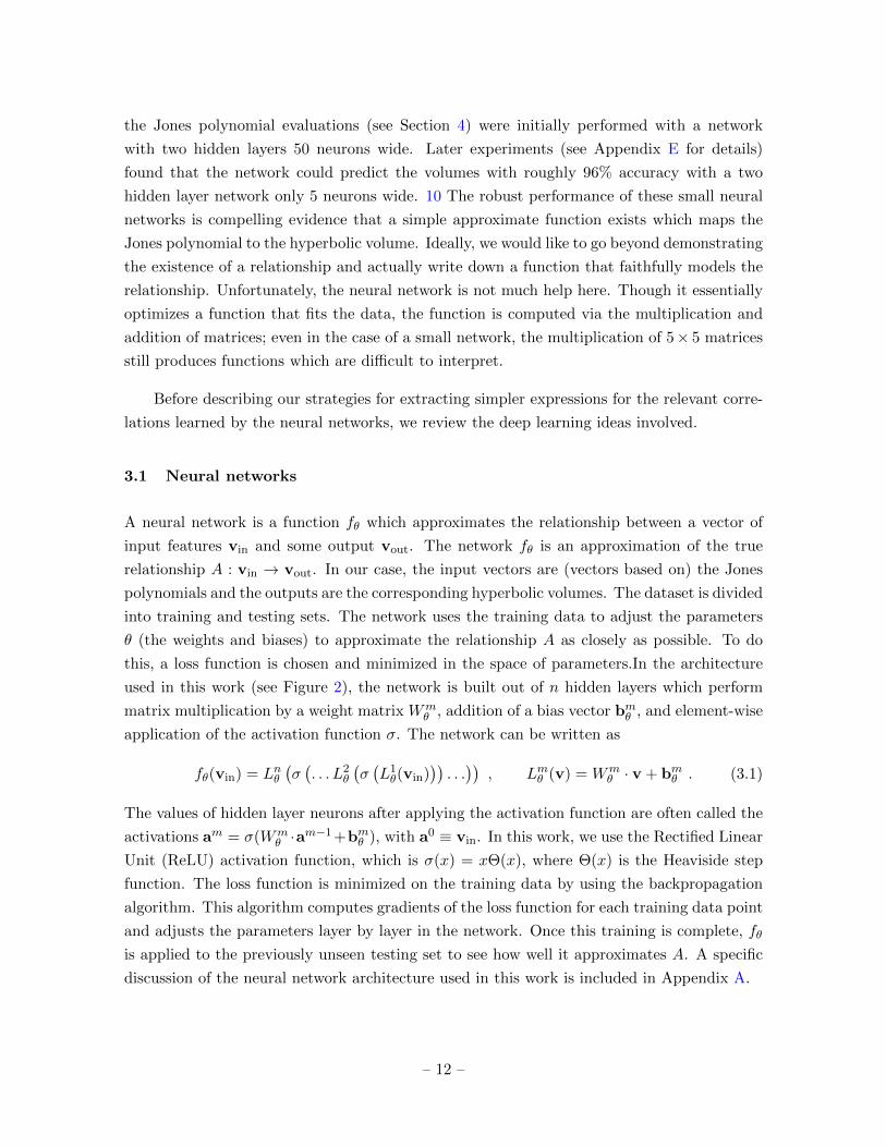
this, a loss function is chosen and minimized in the space of parameters.In the architecture

used in this work (see Figure 2), the network is built out of n hidden layers which perform

matrix multiplication by a weight matrix Wmθ , addition of a bias vector bmθ , and element-wise

application of the activation function σ. The network can be written as

fθ(vin) = Lnθ(σ(. . . L2

θ

(σ(L1θ(vin)

)). . .))

, Lmθ (v) = Wmθ · v + bmθ . (3.1)

The values of hidden layer neurons after applying the activation function are often called the

activations am = σ(Wmθ ·am−1+bmθ ), with a0 ≡ vin. In this work, we use the Rectified Linear

Unit (ReLU) activation function, which is σ(x) = xΘ(x), where Θ(x) is the Heaviside step

function. The loss function is minimized on the training data by using the backpropagation

algorithm. This algorithm computes gradients of the loss function for each training data point

and adjusts the parameters layer by layer in the network. Once this training is complete, fθ

is applied to the previously unseen testing set to see how well it approximates A. A specific

discussion of the neural network architecture used in this work is included in Appendix A.

– 12 –

Figure 2: An example of a two hidden layer fully connected neural network architecture. Each

hidden layer represents matrix multiplication by a weight vector, the addition of a bias vector, and the

element-wise application of an activation function, which introduces non-linearity into the function.

In this work we used the Rectified Linear Unit (ReLU) activation function.

3.2 Layer-wise relevance propagation

Layer-wise relevance propagation (LRP) is a technique which attempts to explain neural

network predictions by calculating a relevance score for each input feature [31]. This is a

useful tool when attempting to derive an analytic function: we can determine which input

variables typically carry the most importance when predicting the output. This allows us to

hypothesize how to weight input variables in our function and perhaps reduce the complexity

of the problem by eliminating redundant variables.

LRP propagates backwards through a neural network, starting at the output layer. The

LRP algorithm redistributes the relevance scores from the current layer into the previous

layer, employing a conservation property. Denote the activation of a neuron i in layer m by

ami . Suppose we have all the relevance scores for the current layer, and want to determine

the scores Rm−1j in the previous layer. The most basic LRP rule calculates these relevance

scores using the formula [32]

Rm−1j =∑k

am−1j Wmjk +N−1m−1b

mk∑

l am−1l Wm

lk + bmkRmk , (3.2)

where the mth layer has Nm neurons. The subscripts on the weights W and biases b here

denote matrix and vector indices. The numerator is the activation of the jth neuron in layer

m− 1, multiplied by the weight matrix element connecting that neuron to neuron k in layer

m to model how much neuron j contributes to the relevance of neuron k. This fraction is

then multiplied by the relevance of neuron k in the layer m. Once the input layer (layer zero)

is reached, the propagation is terminated, and the result is a list of relevance scores for the

– 13 –

input variables. The sum in the denominator runs over all of the neurons in layer m− 1, plus

the bias in layer m: it imposes the conservation property because we begin with Rn = 1 at

the output layer and always preserve ∑k

Rmk = 1 . (3.3)

This methodology was originally proposed in a classifier problem; we have adapted it to the

case of regression.

3.3 Strategies for analyzing the network

Armed with the evidence that our function exists, how do we proceed? The input is too

complicated for educated guesswork or traditional curve fitting techniques, as our encoding of

the Jones polynomial is a 16-vector.16 Our approach involves performing experiments through

which we can probe how the neural network makes its predictions. As stated previously, a

neural network’s inner workings are largely inaccessible. Despite this, by studying a network’s

success when faced with a transformed or truncated form of the Jones polynomial, we can

begin to update our idea of what the eventual function might look like. There are three main

ways that we accomplish this.

The first type of experiment is training a neural network on some truncated or mutated

form of the input data. For instance, inspired by the volume-ish theorem [33], we could

create a new input vector containing just the degrees of the polynomial and the first and

last coefficients: (pmin, pmax, c1, c−1). If the neural network was then still able to learn the

volume, with comparable accuracy to the original experiment, then perhaps our function

could be built from these four numbers. It turns out that the neural network did not perform

well with this input. Another example of this method is detailed in Section 4.

The second strategy is taking a neural network which has already been trained and

feeding it altered input data. For instance, if we train a network on our original 16-vectors

and give it an input vector where certain elements have been zeroed out or shifted by some

constant, can it still predict the volume? This allows us to probe our function for, among other

things, redundant variables and invariance under translations. We could, for example, shift

pairs of input variables by a constant and record the network’s ability to predict the volume.

16In [16], we provided the degrees of the Jones polynomial as inputs. As we explicate in Appendix E.2, the

neural network performs just as well with the coefficients alone. This is the 16-vector to which we refer.

– 14 –

These experiments are inspired by [34], where symbolic regression and machine learning are

approached with a physicist’s methodology.17

Together with these two experiments, we use LRP to understand the relevance of the

various input features in making a prediction. As we reviewed above, LRP is an algorithm

which uses the neuron activations, along with the weight and bias matrices, to map the

activations in the final network layer back onto the input layer. This technique is successfully

implemented in Section 4 to further reduce the number of input variables needed to predict

the volume, eventually yielding formulas with just a handful of numerical parameters and a

single nonlinearity.

4 An approximation formula for the hyperbolic volume

Our goal is to employ the machine learning techniques reviewed in Section 3 to determine what

particular property of the Jones polynomial was exploited by the neural network in [16] to

compute the hyperbolic volume. Inspired by the observations of [18] concerning the analytic

continuation of Chern–Simons theory that we briefly summarized in Section 2, we approach

this task by evaluating the Jones polynomial at various roots of unity. Indeed, the Jones

polynomial is determined by its values at roots of unity, so we lose no essential information

if we include enough such evaluations. We use techniques from interpretable deep learning

to reverse engineer neural networks in Section 4.1 and comment on the implications for the

path integral of analytically continued Chern–Simons theory in Section 4.2.

4.1 Interpretable deep learning

We begin by training a neural network composed of two fully connected hidden layers with

50 neurons each on the Jones polynomial evaluated at e2πip/(r+2), for integers r ∈ [3, 20]

and p ∈ [0, r + 2]. Complex conjugates are omitted from this tabulation since Laurent

polynomials obey J2(K; q) = J2(K; q). The input data (which includes all hyperbolic knots

up to and including 15 crossings) is represented as a vector where the entries at position 2p

and 2p+1 correspond to the real and complex parts of the pth evaluation. Layer-wise relevance

propagation (LRP) [31, 32] is used to identify which evaluations of the Jones polynomial are

important in calculating the volume.18

17We explore symbolic regression techniques further in Appendix E.4. We obtain 96.56% accuracy, but the

formulæ are not obviously interpretable.18Layer-wise relevance propagation has not been widely applied in the physics context, but see [35] for an

example.

– 15 –

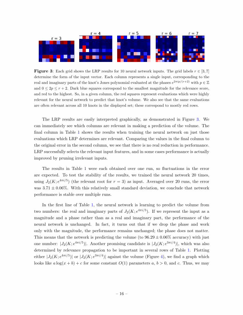
Figure 3: Each grid shows the LRP results for 10 neural network inputs. The grid labels r ∈ [3, 7]

determine the form of the input vector. Each column represents a single input, corresponding to the

real and imaginary parts of the knot’s Jones polynomial evaluated at the phases e2πip/(r+2) with p ∈ Zand 0 ≤ 2p ≤ r + 2. Dark blue squares correspond to the smallest magnitude for the relevance score,

and red to the highest. So, in a given column, the red squares represent evaluations which were highly

relevant for the neural network to predict that knot’s volume. We also see that the same evaluations

are often relevant across all 10 knots in the displayed set; these correspond to mostly red rows.

The LRP results are easily interpreted graphically, as demonstrated in Figure 3. We

can immediately see which columns are relevant in making a prediction of the volume. The

final column in Table 1 shows the results when training the neural network on just those

evaluations which LRP determines are relevant. Comparing the values in the final column to

the original error in the second column, we see that there is no real reduction in performance.

LRP successfully selects the relevant input features, and in some cases performance is actually

improved by pruning irrelevant inputs.

The results in Table 1 were each obtained over one run, so fluctuations in the error

are expected. To test the stability of the results, we trained the neural network 20 times,

using J2(K; e4πi/5) (the relevant root for r = 3) as input. Averaged over 20 runs, the error

was 3.71 ± 0.06%. With this relatively small standard deviation, we conclude that network

performance is stable over multiple runs.

In the first line of Table 1, the neural network is learning to predict the volume from

two numbers: the real and imaginary parts of J2(K; e4πi/5). If we represent the input as a

magnitude and a phase rather than as a real and imaginary part, the performance of the

neural network is unchanged. In fact, it turns out that if we drop the phase and work

only with the magnitude, the performance remains unchanged; the phase does not matter.

This means that the network is predicting the volume (to 96.29± 0.06% accuracy) with just

one number: |J2(K; e4πi/5)|. Another promising candidate is |J2(K; e3πi/4)|, which was also

determined by relevance propagation to be important in several rows of Table 1. Plotting

either |J2(K; e4πi/5)| or |J2(K; e3πi/4)| against the volume (Figure 4), we find a graph which

looks like a log(x+ b) + c for some constant O(1) parameters a, b > 0, and c. Thus, we may

– 16 –

r Error Relevant roots Fractional levels Error (relevant roots)

3 3.48% e4πi/5 12 3.8%

4 6.66% −1 0 6.78%

5 3.48% e6πi/7 13 3.38%

6 2.94% e3πi/4, −1 23 , 0 3%

7 5.37% e8πi/9 14 5.32%

8 2.50% e3πi/5, e4πi/5, −1 43 , 1

2 , 0 2.5%

9 2.74% e8πi/11, e10πi/11 34 , 1

5 2.85%

10 3.51% e2πi/3,e5πi/6, −1 1, 25 , 0 4.39%

11 2.51% e8πi/13, e10πi/13, e12πi/13 54 , 3

5 , 16 2.44%

12 2.39% e5πi/7, e6πi/7, −1 45 , 1

3 , 0 2.75%

13 2.52% e2πi/3, e4πi/5, e14πi/15 1, 12 , 1

7 2.43%

14 2.58% e3πi/4, e7πi/8, −1 23 , 2

7 , 0 2.55%

15 2.38% e12πi/17, e14πi/17, e16πi/17 56 , 3

7 , 18 2.4%

16 2.57% e2πi/3, e7πi/9, e8πi/9, −1 1, 47 , 1

4 , 0 2.45%

17 2.65% e14πi/19, e16πi/19, e18πi/19, 57 , 3

8 , 19 2.46%

18 2.49% e4πi/5, e9πi/10, −1 12 , 2

9 , 0 2.52%

19 2.45% e2πi/3, e16πi/21, e6πi/7, e20πi/21 1, 58 , 1

3 , 110 2.43%

20 2.79% e8πi/11, e9πi/11, e10πi/11, −1 34 , 4

9 , 15 , 0 2.4%

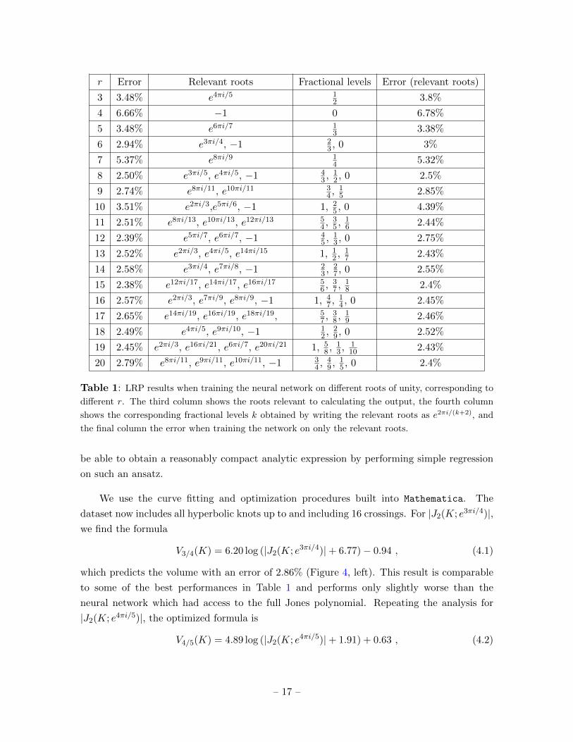
Table 1: LRP results when training the neural network on different roots of unity, corresponding to

different r. The third column shows the roots relevant to calculating the output, the fourth column

shows the corresponding fractional levels k obtained by writing the relevant roots as e2πi/(k+2), and

the final column the error when training the network on only the relevant roots.

be able to obtain a reasonably compact analytic expression by performing simple regression

on such an ansatz.

We use the curve fitting and optimization procedures built into Mathematica. The

dataset now includes all hyperbolic knots up to and including 16 crossings. For |J2(K; e3πi/4)|,we find the formula

V3/4(K) = 6.20 log (|J2(K; e3πi/4)|+ 6.77)− 0.94 , (4.1)

which predicts the volume with an error of 2.86% (Figure 4, left). This result is comparable

to some of the best performances in Table 1 and performs only slightly worse than the

neural network which had access to the full Jones polynomial. Repeating the analysis for

|J2(K; e4πi/5)|, the optimized formula is

V4/5(K) = 4.89 log (|J2(K; e4πi/5)|+ 1.91) + 0.63 , (4.2)

– 17 –

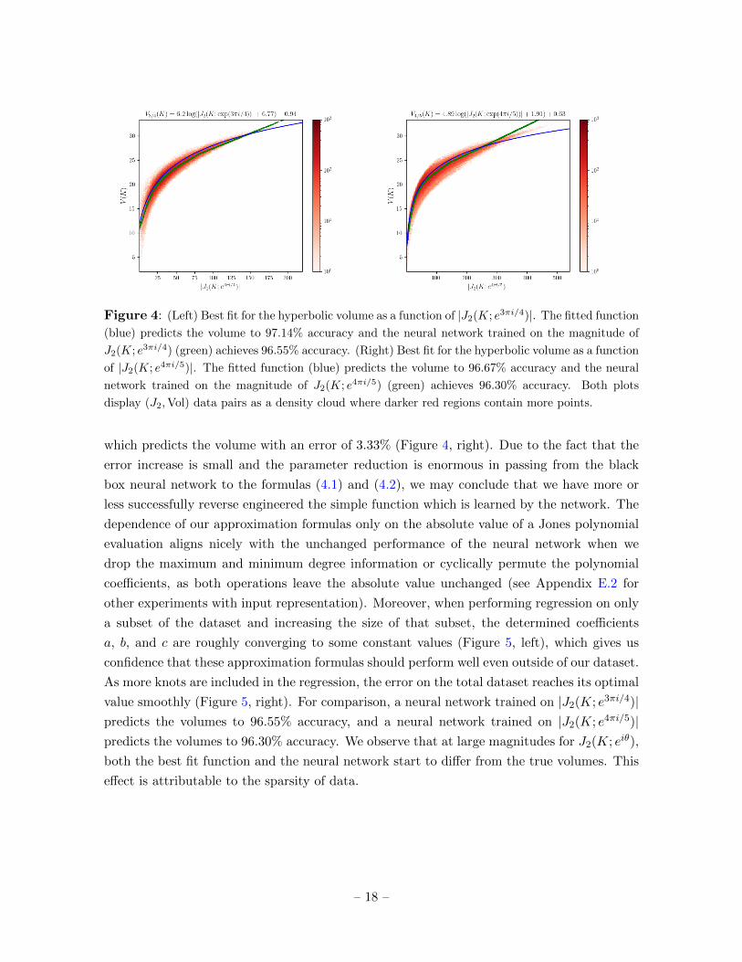
Figure 4: (Left) Best fit for the hyperbolic volume as a function of |J2(K; e3πi/4)|. The fitted function

(blue) predicts the volume to 97.14% accuracy and the neural network trained on the magnitude of

J2(K; e3πi/4) (green) achieves 96.55% accuracy. (Right) Best fit for the hyperbolic volume as a function

of |J2(K; e4πi/5)|. The fitted function (blue) predicts the volume to 96.67% accuracy and the neural

network trained on the magnitude of J2(K; e4πi/5) (green) achieves 96.30% accuracy. Both plots

display (J2,Vol) data pairs as a density cloud where darker red regions contain more points.

which predicts the volume with an error of 3.33% (Figure 4, right). Due to the fact that the

error increase is small and the parameter reduction is enormous in passing from the black

box neural network to the formulas (4.1) and (4.2), we may conclude that we have more or

less successfully reverse engineered the simple function which is learned by the network. The

dependence of our approximation formulas only on the absolute value of a Jones polynomial

evaluation aligns nicely with the unchanged performance of the neural network when we

drop the maximum and minimum degree information or cyclically permute the polynomial

coefficients, as both operations leave the absolute value unchanged (see Appendix E.2 for

other experiments with input representation). Moreover, when performing regression on only

a subset of the dataset and increasing the size of that subset, the determined coefficients

a, b, and c are roughly converging to some constant values (Figure 5, left), which gives us

confidence that these approximation formulas should perform well even outside of our dataset.

As more knots are included in the regression, the error on the total dataset reaches its optimal

value smoothly (Figure 5, right). For comparison, a neural network trained on |J2(K; e3πi/4)|predicts the volumes to 96.55% accuracy, and a neural network trained on |J2(K; e4πi/5)|predicts the volumes to 96.30% accuracy. We observe that at large magnitudes for J2(K; eiθ),

both the best fit function and the neural network start to differ from the true volumes. This

effect is attributable to the sparsity of data.

– 18 –

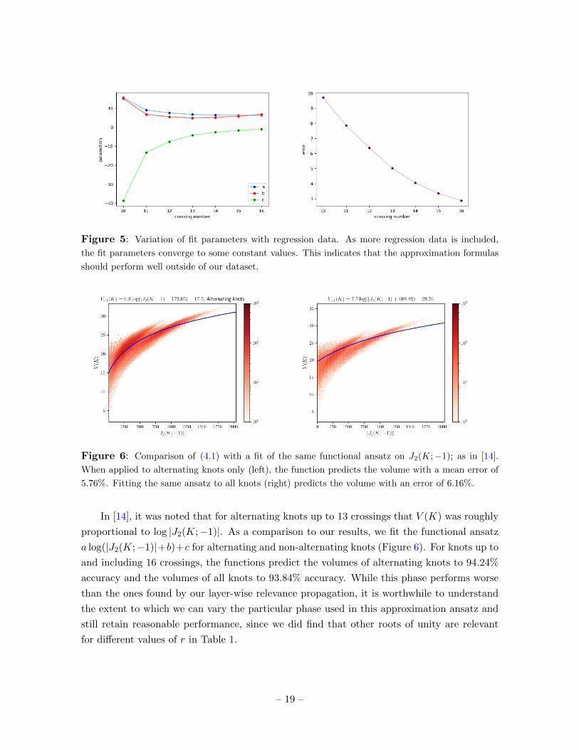
Figure 5: Variation of fit parameters with regression data. As more regression data is included,

the fit parameters converge to some constant values. This indicates that the approximation formulas

should perform well outside of our dataset.

Figure 6: Comparison of (4.1) with a fit of the same functional ansatz on J2(K;−1); as in [14].

When applied to alternating knots only (left), the function predicts the volume with a mean error of

5.76%. Fitting the same ansatz to all knots (right) predicts the volume with an error of 6.16%.

In [14], it was noted that for alternating knots up to 13 crossings that V (K) was roughly

proportional to log |J2(K;−1)|. As a comparison to our results, we fit the functional ansatz

a log(|J2(K;−1)|+b)+c for alternating and non-alternating knots (Figure 6). For knots up to

and including 16 crossings, the functions predict the volumes of alternating knots to 94.24%

accuracy and the volumes of all knots to 93.84% accuracy. While this phase performs worse

than the ones found by our layer-wise relevance propagation, it is worthwhile to understand

the extent to which we can vary the particular phase used in this approximation ansatz and

still retain reasonable performance, since we did find that other roots of unity are relevant

for different values of r in Table 1.

– 19 –

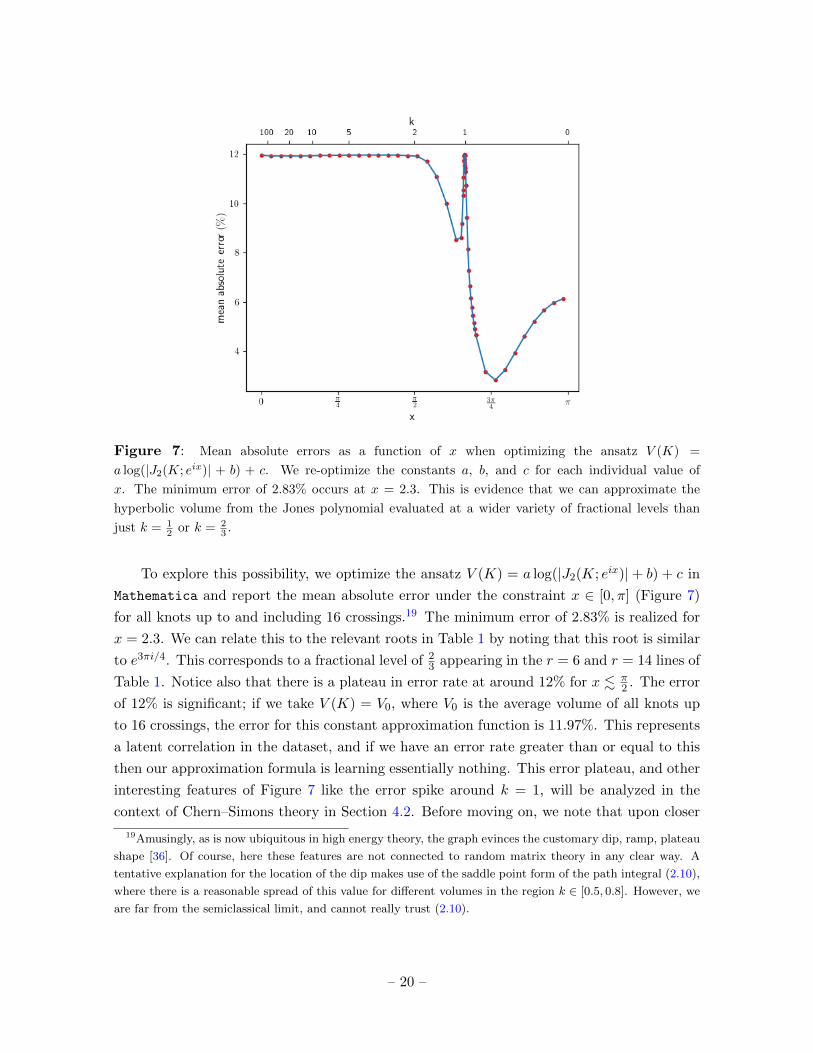
Figure 7: Mean absolute errors as a function of x when optimizing the ansatz V (K) =

a log(|J2(K; eix)| + b) + c. We re-optimize the constants a, b, and c for each individual value of

x. The minimum error of 2.83% occurs at x = 2.3. This is evidence that we can approximate the

hyperbolic volume from the Jones polynomial evaluated at a wider variety of fractional levels than

just k = 12 or k = 2

3 .

To explore this possibility, we optimize the ansatz V (K) = a log(|J2(K; eix)|+ b) + c in

Mathematica and report the mean absolute error under the constraint x ∈ [0, π] (Figure 7)

for all knots up to and including 16 crossings.19 The minimum error of 2.83% is realized for

x = 2.3. We can relate this to the relevant roots in Table 1 by noting that this root is similar

to e3πi/4. This corresponds to a fractional level of 23 appearing in the r = 6 and r = 14 lines of

Table 1. Notice also that there is a plateau in error rate at around 12% for x . π2 . The error

of 12% is significant; if we take V (K) = V0, where V0 is the average volume of all knots up

to 16 crossings, the error for this constant approximation function is 11.97%. This represents

a latent correlation in the dataset, and if we have an error rate greater than or equal to this

then our approximation formula is learning essentially nothing. This error plateau, and other

interesting features of Figure 7 like the error spike around k = 1, will be analyzed in the

context of Chern–Simons theory in Section 4.2. Before moving on, we note that upon closer

19Amusingly, as is now ubiquitous in high energy theory, the graph evinces the customary dip, ramp, plateau

shape [36]. Of course, here these features are not connected to random matrix theory in any clear way. A

tentative explanation for the location of the dip makes use of the saddle point form of the path integral (2.10),

where there is a reasonable spread of this value for different volumes in the region k ∈ [0.5, 0.8]. However, we

are far from the semiclassical limit, and cannot really trust (2.10).

– 20 –

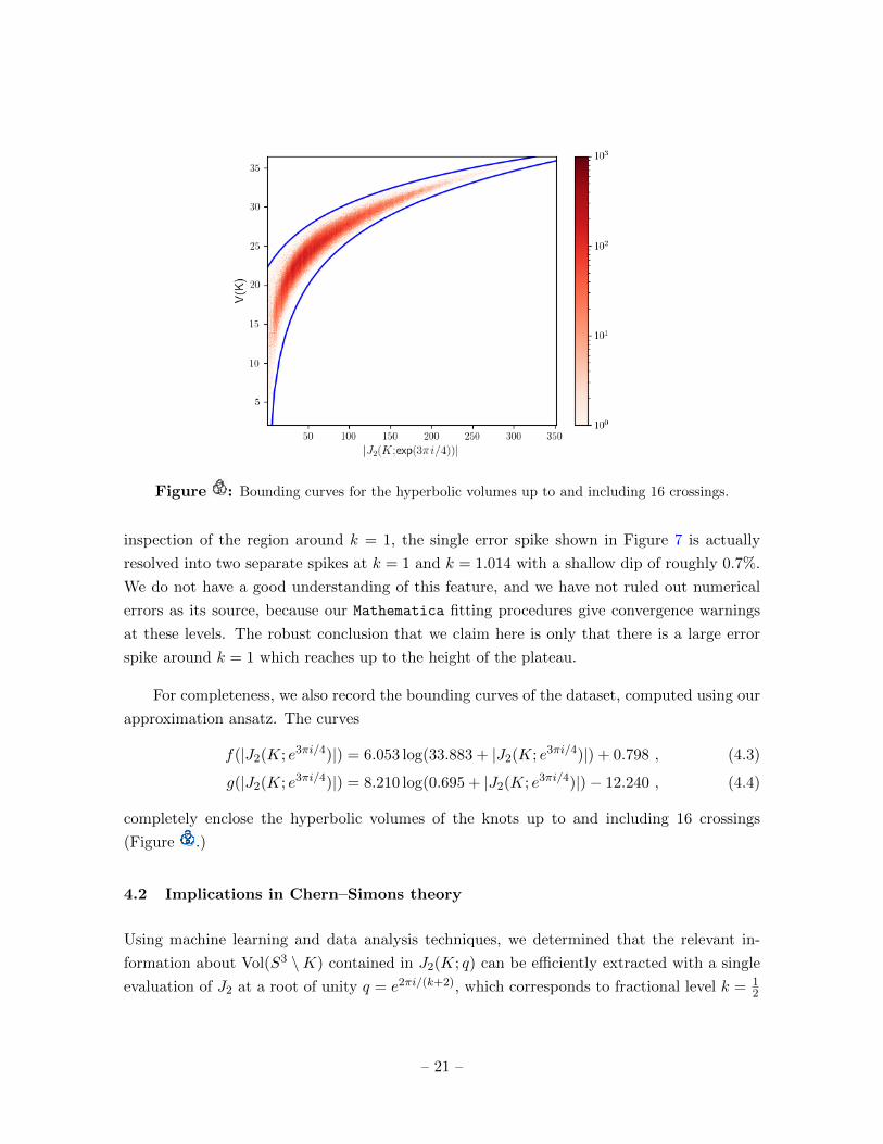
Figure : Bounding curves for the hyperbolic volumes up to and including 16 crossings.

inspection of the region around k = 1, the single error spike shown in Figure 7 is actually

resolved into two separate spikes at k = 1 and k = 1.014 with a shallow dip of roughly 0.7%.

We do not have a good understanding of this feature, and we have not ruled out numerical

errors as its source, because our Mathematica fitting procedures give convergence warnings

at these levels. The robust conclusion that we claim here is only that there is a large error

spike around k = 1 which reaches up to the height of the plateau.

For completeness, we also record the bounding curves of the dataset, computed using our

approximation ansatz. The curves

f(|J2(K; e3πi/4)|) = 6.053 log(33.883 + |J2(K; e3πi/4)|) + 0.798 , (4.3)

g(|J2(K; e3πi/4)|) = 8.210 log(0.695 + |J2(K; e3πi/4)|)− 12.240 , (4.4)

completely enclose the hyperbolic volumes of the knots up to and including 16 crossings

(Figure .)

4.2 Implications in Chern–Simons theory

Using machine learning and data analysis techniques, we determined that the relevant in-

formation about Vol(S3 \K) contained in J2(K; q) can be efficiently extracted with a single

evaluation of J2 at a root of unity q = e2πi/(k+2), which corresponds to fractional level k = 12

– 21 –

or k = 23 . At k = 2

3 , for example, we have q = e3πi/4, and we find that the simple function (1.2)

reproduces the hyperbolic volume of K with almost no loss of accuracy compared to the full

neural network of [16]. The fractional level k = 12 has been studied in the context of Abelian

Chern–Simons theory [37], but has not played a significant role in the non-Abelian theory we

study here, and level k = 23 (to our knowledge) has hardly been studied at all. Of course, due

to gauge invariance, non-Abelian Chern–Simons theory cannot be defined in the naıve way

at fractional level, and it is for this reason that the analytic continuation techniques of [18]

have an intriguing bearing on our observations.

Our numerical results suggest the Lefschetz thimbles involved in the analytically contin-

ued path integral at γ = 2 or γ = 32 are somehow related to the set of thimbles which appear

semiclassically at γ = 1. Perhaps the set of relevant thimbles around γ ∈ (32 , 2) contains

the geometric conjugate SL(2,C) connection that we expect semiclassically at γ = 1.20 This

interpretation suggests that the geometric conjugate connection contributes to the path in-

tegral for the maximum number of knots in our dataset around γ = 32 , or k = 2

3 , since that

is where the approximation formula performs optimally. This location coincides with the

bottom of the dip in Figure 7. Similarly, the ramp between 23 < k < 2 (ignoring the spike at

k = 1) is consistent with the interpretation that large fractions of knots are beginning to lose

the geometric conjugate connection for k > 23 . That the dip begins at k = 0 with an error

rate which is already fairly low may signal that many knots retain the geometric conjugate

connection even as γ becomes large.

We must emphasize that we are not working in the semiclassical limit of large n and

k. Instead, we are actually in the opposite limit where both quantities are O(1). Therefore,

quantum effects in the path integral are strong, and it is not clear how to isolate the con-

tribution of the critical points. Nevertheless, it seems that our machine learning techniques

suggest this is approximately possible with some simple processing of the path integral result.

This phenomenon is a bit reminiscent of the ease with which one-loop quantum corrections

are incorporated in Chern–Simons theory, through a simple shift k → k+ 2 and n→ n+ 1 in

the semiclassical formulas. Here, we have an effect at the level of the analytically continued

path integral, where a simple multiplication and shift can absorb quantum corrections to a

reasonable degree. It would be interesting to try to make this precise.

20The geometric conjugate connection is a flat SL(2,C) connection which has Im(W ) = −Vol(M)/2π, which

is necessary for the factors of i to cancel and yield ekVol(M)/2π in a saddle point approximation of |Z(M)| or the

analytic continuation of |Z(M)|. It is simply the complex conjugate of the geometric connection we mentioned

previously. To prevent any ambiguity, we remark that the object called A+ in (5.61) of [18] is an instance of

what we are calling the geometric conjugate connection.

– 22 –

It is also instructive to study the error spike at k = 1 in Figure 7. Readers familiar with

the main message of [18] will understand why this feature is in fact expected: at integer values

of the Chern–Simons level with k+ 1 ≥ n, the path integral ratio (2.6) receives contributions

only from SU(2)-valued critical points, and can be analyzed using the original techniques

in [10]. In other words, the SU(2)k current algebra has an integrable representation of

dimension n = k+ 1, and so the techniques of [10] are sufficient and no analytic continuation

is necessary. Of course, at n = k + 2, there is a vanishing of the bare path integral, but the

ratio (2.6) remains finite and is sensitive to the volume like the analytically continued bare

path integral. That this occurs only at the special value n = k+ 2 and not for any n < k+ 2

essentially follows from the fact that the bare expectation value of the unknot does not vanish

for 0 < n < k + 2 with integer k.

This observation supports our interpretation that the presence of the geometric conjugate

connection is responsible for the approximation formula’s success. In this case, we cannot

expect to learn anything about the hyperbolic volume at k = 1 and n = 2 beyond latent

correlations in the dataset because the geometric conjugate connection does not contribute

to the path integral there. Even if it is present in the numerator of (2.6), it will cancel with

another contribution for integer k > n − 2, and so our approximation formula performs as

poorly as possible at k = 1. However, there are sharp improvements to the approximation

formula just below or above this value, where k again becomes fractional and we may find a

contribution from the geometric conjugate connection.

Intriguingly, there seems to be a transition around γ = 23 (equivalently, k = 3

2) where the

approximation formulas begin to improve over the maximum error, and [18] found that the

geometric conjugate connection for the figure-eight knot is added to the path integral by a

Stokes phenomenon precisely at this value. The appearance of this maximum error plateau,

which roughly matches the error of taking a constant approximation function equal to the

average volume in the dataset, is consistent with the interpretation that the approximation

formula with k > 32 fails to convey anything useful because the geometric conjugate connection

is completely absent from the numerator of (2.6), rather than being present and canceling for

integer k. Perhaps there is a larger class of knots with a Stokes phenomenon at γ = 23 which

adds the geometric conjugate connection to the path integral, and there are only a few knots

(or perhaps none at all) which receive such a contribution for k > 32 .

If we follow the suggestion that the success of our approximation formula is signalling

the presence of the geometric conjugate connection for most knots in the dataset, we are led

to an interesting observation concerning the volume conjecture. As discussed previously, it is

well known that the volume conjecture does not converge monotonically in n [15]. Perhaps

– 23 –

the reason for this is that the geometric conjugate connection is missing for early terms in the

sequence, and appears at a certain point, after which convergence is monotonic. For example,

the first term in the sequence involves |J2(K;−1)|, which corresponds to k = 0 and therefore

γ = ∞. While it may be that some knots acquire the geometric conjugate contribution by

γ = 1 and never lose it for any γ > 1, this may not be the case for all knots. If the geometric

conjugate connection is lost by Stokes phenomena at some γ > 1, the first term in the volume

conjecture sequence cannot be expected to be a good approximation. We comment further

on this in Section 5.

5 Discussion

In this work, we have utilized neural networks and layer-wise relevance propagation to extract

a very simple function V (K) which predicts with better than 97% accuracy the volume of a

hyperbolic knot using only a single evaluation of the Jones polynomial at a root of unity. The

existence of such a function was predicted in [16], and prior related observations had also been

suggestive [14, 38]. The main problem described at the end of [16] was to determine what

simple function was being computed by a neural network, and the roughly equal accuracy

of our simple function and the neural network is strong evidence that we have succeeded.

We also found excellent alignment between the form of the approximation ansatz and the

operations on the inputs (dropping degree information, cyclic coefficient permutations) which

left the network performance unchanged.

We commented briefly on the implications of this result for analytically continued Chern–

Simons theory in Section 4.2. It is clear that there is at least some connection, because the

root of unity involved in the calculation is not accessible by the standard definition of the

path integral: it corresponds to fractional level k. However, precisely what is gained by

studying the path integral far from the semiclassical limit around γ = 32 or γ = 2, and why

this should be related to the semiclassical limit near γ = 1, is not at all clear. Our usual

intuition from quantum field theory suggests that the strong quantum effects at small k ought

to completely mask the particular value of the action at the geometric conjugate connection.

Mysteriously, this does not happen, and (at least, e.g., for large |J2(K; e3πi/4)|) there is

an essentially universal way to extract the saddle point value of this particular connection

with high accuracy for any hyperbolic knot. We have found some supporting evidence for

our interpretation that the success of the approximation formula signals the presence of the

geometric conjugate connection in most knots in our dataset. This evidence involved the

spike in error near the integer k = 1 as well as the rough matching between the location of

– 24 –

the relevant Stokes phenomenon for the figure-eight knot and the critical value of γ where

the approximation formula begins to perform well.

An interesting future direction would be to try to derive an inequality, along the lines

of the volume-ish theorem [33], using analytically continued Chern–Simons theory. Indeed,

the volume-ish theorem should generalize to higher colors, with the upper and lower bounds

converging in the infinite n-limit. Deducing an inequality seems quite difficult, as the analysis

is very involved for each individual knot [18]. Nevertheless, we may hope to find some unifying

theme now that we have a specific location of interest (further along the real γ axis than

previously suspected). As a very first step, one would have to understand how to evaluate

the full path integral on the relevant Lefschetz thimbles in order to bound the contributions

of other critical points.

We observed in Section 4.2 that there could be large discrepancies between the value of

γ for the early terms in the volume conjecture and the value of γ at which the geometric

conjugate connection is added to the path integral. This motivates a new style of volume

conjecture which could be engineered to be immediately monotonic. We simply keep γ ≈ 1

throughout the limit, though this must be done to carefully avoid integer level. By avoiding

integer level, we mean that, e.g., for n = 2, if we simply solve γ = 1 we find k = 1, and we

already argued why this evaluation should yield no nontrivial information about the volume.

So we must instead begin at some value like γ = 2, which would correspond to k = 12 .

Moreover, we should tune this value with n so that we approach γ = 1 in the semiclassical

limit. All these constraints lead to a version of the volume conjecture where we evaluate the

relevant path integrals at a candidate value of γ such as

γ =n

n− 1. (5.1)

This corresponds to level

k =(n− 1)2

n, (5.2)

which is certainly always fractional for integer n ≥ 2 since the parities of the numerator and

denominator do not match. With this choice, a monotonic version of the volume conjecture

would be (recalling that the prefactor 2πn in the usual volume conjecture is really 2π

k from the

Chern–Simons perspective)

limn→∞

2πn log |Jn(K; e2πin/(n2+1))|

(n− 1)2= Vol(S3 \K) . (5.3)

This conjecture repairs the non-monotonicity in the volume conjecture sequence for the figure-

eight knot (Figure 9). Of course, we are not guaranteed that all knots still receive a con-

tribution from the geometric conjugate connection at γ = 2. Indeed, unfortunately, (5.3)

– 25 –

5 10 15 20

2

4

6

8

10

12

14

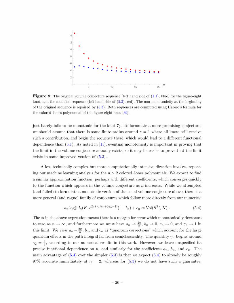
Figure 9: The original volume conjecture sequence (left hand side of (1.1), blue) for the figure-eight

knot, and the modified sequence (left hand side of (5.3), red). The non-monotonicity at the beginning

of the original sequence is repaired by (5.3). Both sequences are computed using Habiro’s formula for

the colored Jones polynomial of the figure-eight knot [39].

just barely fails to be monotonic for the knot 72. To formulate a more promising conjecture,

we should assume that there is some finite radius around γ = 1 where all knots still receive

such a contribution, and begin the sequence there, which would lead to a different functional

dependence than (5.1). As noted in [15], eventual monotonicity is important in proving that

the limit in the volume conjecture actually exists, so it may be easier to prove that the limit

exists in some improved version of (5.3).

A less technically complex but more computationally intensive direction involves repeat-

ing our machine learning analysis for the n > 2 colored Jones polynomials. We expect to find

a similar approximation function, perhaps with different coefficients, which converges quickly

to the function which appears in the volume conjecture as n increases. While we attempted

(and failed) to formulate a monotonic version of the usual volume conjecture above, there is a

more general (and vague) family of conjectures which follow more directly from our numerics:

an log(|Jn(K; e2πiγn/(n+2γn−1))|+ bn) + cn ≈ Vol(S3 \K) . (5.4)

The ≈ in the above expression means there is a margin for error which monotonically decreases

to zero as n → ∞, and furthermore we must have an → 2πn , bn → 0, cn → 0, and γn → 1 in

this limit. We view an− 2πn , bn, and cn as “quantum corrections” which account for the large

quantum effects in the path integral far from semiclassicality. The quantity γn begins around

γ2 = 32 , according to our numerical results in this work. However, we leave unspecified its

precise functional dependence on n, and similarly for the coefficients an, bn, and cn. The

main advantage of (5.4) over the simpler (5.3) is that we expect (5.4) to already be roughly

97% accurate immediately at n = 2, whereas for (5.3) we do not have such a guarantee.

– 26 –

Indeed, we expect that the error in (5.4) is actually bounded, whereas (5.3) can be arbitrarily

wrong at small n, though an improved version of (5.3) would still converge monotonically in

n. Of course, the price we pay for this immediate accuracy is the introduction of many free

parameters in the conjecture.

Acknowledgments

We are grateful to Onkar Parrikar for prior collaboration in machine learning aspects of

knot theory. Figure 1 was obtained in this joint work. We thank Nathan Dunfield, Sergei

Gukov, Yang-Hui He, Onkar Parrikar, and Edward Witten for discussions and comments on

the manuscript. We thank Dror Bar-Natan for computing HOMFLY-PT polynomials at 15

crossings and for the dbnsymb LATEX symbol package [40]. JC and VJ are supported by the

South African Research Chairs Initiative of the Department of Science and Technology and

the National Research Foundation and VJ by a Simons Foundation Mathematics and Physical

Sciences Targeted Grant, 509116. AK is supported by the Simons Foundation through the

It from Qubit Collaboration and thanks the University of Pennsylvania, where this work was

initiated.

A Basic neural network setup

The neural networks used in these experiments were built in Python 3, using GPU-Tensorflow

with a Keras wrapper [41]. The neural network has two hidden layers, 100 neurons wide,

with ReLU activation functions. The training used an Adam optimizer and a mean squared

loss function. There were typically 100 training epochs. The network was trained on 10% of

the 313, 209 knots up to (and including) 15 crossings and tested on the remaining 90%. The

code snippet below summarizes the key steps of building and training the neural network.

import numpy as np

import t en s o r f l ow as t f

from s k l e a rn . m o d e l s e l e c t i o n import t r a i n t e s t s p l i t

t r a i n j o n e s , t e s t j o n e s , t r a i n v o l s , t e s t v o l s =

t r a i n t e s t s p l i t ( jones , vo l s , t e s t s i z e =0.9)

model = t f . keras . models . Sequent i a l ( [

t f . ke ras . l a y e r s . Dense (100 , a c t i v a t i o n=’ r e l u ’ ,

– 27 –

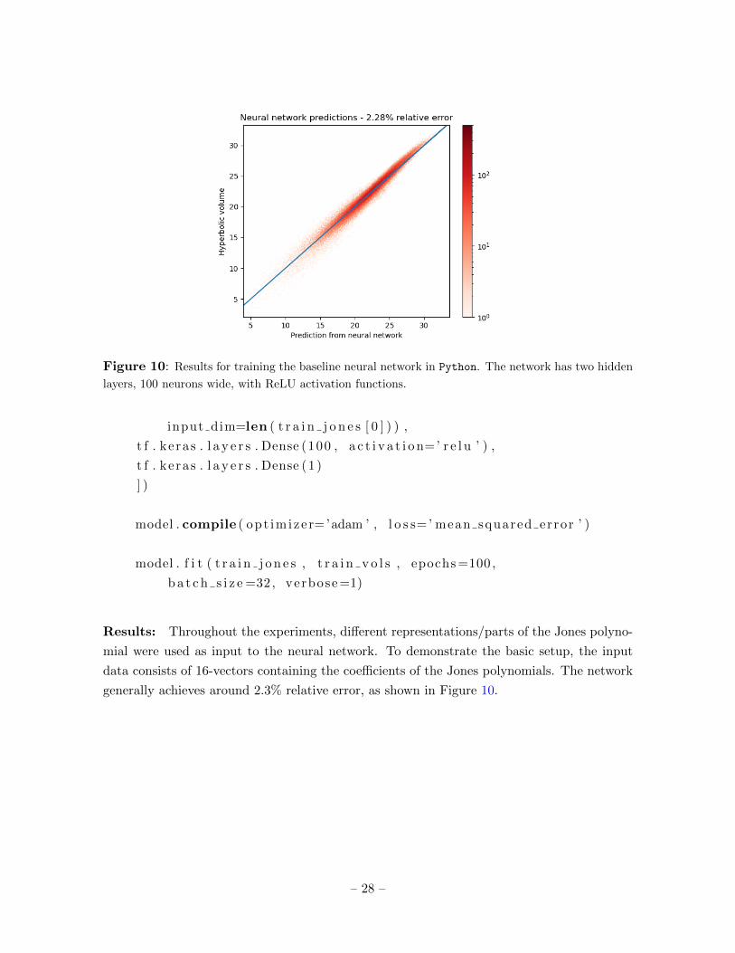
Figure 10: Results for training the baseline neural network in Python. The network has two hidden

layers, 100 neurons wide, with ReLU activation functions.

input dim=len ( t r a i n j o n e s [ 0 ] ) ) ,

t f . ke ras . l a y e r s . Dense (100 , a c t i v a t i o n=’ r e l u ’ ) ,

t f . ke ras . l a y e r s . Dense (1 )

] )

model . compile ( opt imize r=’adam ’ , l o s s=’ mean squared error ’ )

model . f i t ( t r a i n j o n e s , t r a i n v o l s , epochs =100 ,

b a t c h s i z e =32, verbose =1)

Results: Throughout the experiments, different representations/parts of the Jones polyno-

mial were used as input to the neural network. To demonstrate the basic setup, the input

data consists of 16-vectors containing the coefficients of the Jones polynomials. The network

generally achieves around 2.3% relative error, as shown in Figure 10.

– 28 –

B Khovanov homology, Jones coefficients, and volume

B.1 Khovanov homology

Machine learning has been applied to string theory for a variety of purposes, beginning in [42–

45]. Many instances in which machine learning has been successfully applied to mathematical

physics involve an underlying homological structure [46–49].21 In certain cases, analytic for-

mulas inspired by machine learning results have been obtained [55–57]. Knot theory appears

to be no exception to this pattern, as there is an underlying homology theory related to

the Jones polynomial known as Khovanov homology [58]. As we will make reference to the

homological nature of the Jones polynomial at several points in this supplemental discussion,

here we provide a brief explanation of Khovanov homology following the compact treatment

in [59].

The Jones polynomial, in its form more familiar to mathematicians, is a Laurent poly-

nomial in a variable q defined by a skein relation22

(B.1)

where 〈K〉 is known as the Kauffman bracket [60] of the knot K, and n± are the number of

right- and left-handed crossings in a diagram of K. The quantity n+ − n− is often called the

writhe of the knot diagram. We have used the notation J because this object is not quite

equivalent to our J2(K; q). It is unnormalized in the following sense:

J(K; q) = (q + q−1)J2(K; q2) . (B.2)

The skein relation for the Kauffman bracket involves two “smoothings” of a given crossing.

Of course, in each of these smoothings, the total number of crossings is reduced by one. The

recursion terminates when all crossings have been smoothed, so the set of binary strings of

length c, {0, 1}c, is the set of total smoothings for a knot diagram with c crossings.

Khovanov’s homology, roughly speaking, begins by assigning a vector space Vα(K) to

each string α ∈ {0, 1}c. If V is the two-dimensional graded vector space with basis elements

v± and deg(v±) = ±1, then Vα(K) ≡ V ⊗k{r} where the total smoothing α of K results in

21Such structures appear in string theory fairly often, and more sophisticated machine learning (beyond

simple feed-forward network architecture) has also been applied fruitfully to the study of the string landscape.

For a small sample, see [45, 50–53], and also see the review [54] for more complete references in this area.22Knot theorists will notice that this is a rather non-standard skein relation. We will comment on this, and

related normalization issues, in Appendix C.

– 29 –

k closed loops, and {r} is the degree shift by r.23 The height of a string α is defined as

the number of ones, |α| =∑

i αi. The strings with equal height r can be grouped together,

and (through some more work) the corresponding vector spaces can be assembled into a

doubly-graded homology theory Hr(K), with Poincare polynomial

Kh(K; t, q) ≡∑r

trq dimHr(K) . (B.3)

Khovanov proved that this homology theory is a knot invariant, and that its graded Euler

characteristic is the unnormalized Jones polynomial

χq(K) = Kh(K;−1, q) = J(K; q) . (B.4)

Another useful quantity associated with Khovanov homology is the Khovanov rank, given by

rank(H•(K)) =∑r

q dimHr(K) . (B.5)

The Khovanov rank is correlated with the hyperbolic volume, as noticed in [38], and was

compared to neural network prediction techniques in [16].

The main point we wish to convey with this brief summary is that the coefficients of

the Jones polynomial are related to dimensions of homology groups, and therefore any suc-

cess of our machine learning techniques represents another piece of evidence that underly-

ing homological structure is relevant for characterizing physics and mathematics which is

machine-learnable.

B.2 Power law behavior of coefficients

In this appendix, we study how the coefficients in the Jones polynomial may be individually

related to the hyperbolic volume. Through Khovanov homology, we know that each coefficient

is measuring the dimension of a certain homology group. Thus, this numerical study is in

some sense a generalization of Khovanov’s study of patterns in his homology [38], and his

observation that coarser properties of his homology are related to the volume (see [16] for

more explanation and analysis of this point). Patterns in Jones polynomial coefficients were

also studied in [61, 62].

The vectors of coefficients is represented as J = (c1, . . . , c8, c−8, . . . , c−1), where padding

with zeros is done from the center so that, say, c1 is always the first nonzero coefficient in the

23Recall that a graded vector space W = ⊕mWm has graded dimension q dimW =∑m q

m dimWm.

Furthermore, the degree shift produces another graded vector space W{r} with homogeneous subspaces

W{r}m ≡Wm−r, so q dimW{r} =∑m q

m+r dimWm.

– 30 –

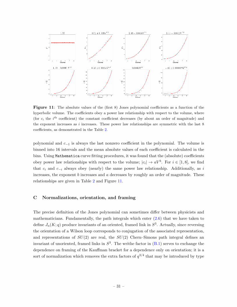
Figure 11: The absolute values of the (first 8) Jones polynomial coefficients as a function of the

hyperbolic volume. The coefficients obey a power law relationship with respect to the volume, where

(for ci the ith coefficient) the constant coefficient decreases (by about an order of magnitude) and

the exponent increases as i increases. These power law relationships are symmetric with the last 8

coefficients, as demonstrated in the Table 2.

polynomial and c−1 is always the last nonzero coefficient in the polynomial. The volume is

binned into 16 intervals and the mean absolute values of each coefficient is calculated in the

bins. Using Mathematica curve fitting procedures, it was found that the (absolute) coefficients

obey power law relationships with respect to the volume; |ci| → aV b. For i ∈ [1, 8], we find

that ci and c−i always obey (nearly) the same power law relationship. Additionally, as i

increases, the exponent b increases and a decreases by roughly an order of magnitude. These

relationships are given in Table 2 and Figure 11.

C Normalizations, orientation, and framing

The precise definition of the Jones polynomial can sometimes differ between physicists and

mathematicians. Fundamentally, the path integrals which enter (2.6) that we have taken to

define Jn(K; q) produce invariants of an oriented, framed link in S3. Actually, since reversing

the orientation of a Wilson loop corresponds to conjugation of the associated representation,

and representations of SU(2) are real, the SU(2) Chern–Simons path integral defines an

invariant of unoriented, framed links in S3. The writhe factor in (B.1) serves to exchange the

dependence on framing of the Kauffman bracket for a dependence only on orientation; it is a

sort of normalization which removes the extra factors of q3/4 that may be introduced by type

– 31 –

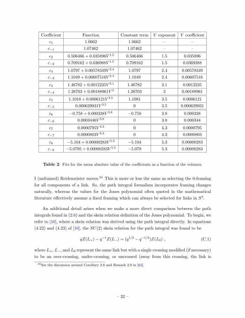
Coefficient Function Constant term V exponent V coefficient

c1 1.0662 1.0662 – –

c−1 1.07462 1.07462 – –

c2 0.506466 + 0.035896V 1.5 0.506466 1.5 0.035896

c−2 0.709162 + 0.036988V 1.5 0.709162 1.5 0.0369388

c3 1.0797 + 0.00578349V 2.4 1.0797 2.4 0.00578349

c−3 1.1049 + 0.00607516V 2.4 1.1049 2.4 0.00607516

c4 1.46782 + 0.0012235V 3.1 1.46782 3.1 0.0012235

c−4 1.26703 + 0.00188961V 3 1.26703 3 0.00188961

c5 1.1018 + 0.0006121V 3.5 1.1081 3.5 0.0006121

c−5 0.000629931V 3.5 0 3.5 0.000629931

c6 −0.758 + 0.000338V 3.8 −0.758 3.8 0.000338

c−6 0.0003446V 3.8 0 3.8 0.000344

c7 0.0000795V 4.3 0 4.3 0.0000795

c−7 0.0000803V 4.3 0 4.3 0.0000803

c8 −5.104 + 0.00000283V 5.3 −5.104 5.3 0.00000283

c−8 −5.0795 + 0.00000283V 5.3 −5.079 5.3 0.00000283

Table 2: Fits for the mean absolute value of the coefficients as a function of the volumes.

I (unframed) Reidemeister moves.24 This is more or less the same as selecting the 0-framing

for all components of a link. So, the path integral formalism incorporates framing changes

naturally, whereas the values for the Jones polynomial often quoted in the mathematical

literature effectively assume a fixed framing which can always be selected for links in S3.

An additional detail arises when we make a more direct comparison between the path

integrals found in (2.6) and the skein relation definition of the Jones polynomial. To begin, we

refer to [10], where a skein relation was derived using the path integral directly. In equations

(4.22) and (4.23) of [10], the SU(2) skein relation for the path integral was found to be

qZ(L+)− q−1Z(L−) = (q1/2 − q−1/2)Z(L0) , (C.1)

where L+, L−, and L0 represent the same link but with a single crossing modified (if necessary)

to be an over-crossing, under-crossing, or uncrossed (away from this crossing, the link is

24See the discussion around Corollary 2.8 and Remark 2.9 in [63].

– 32 –

unchanged). Pictorially, (C.1) is

(C.2)

Other than this relation, the only other piece of information needed to determine the Jones

polynomial (as defined in (2.6)) is the expectation of the unknot. If we normalize the path

integral as in (2.6), the unknot has expectation 1.

J2(01; q) = 1 . (C.3)

This is equivalent to requiring that the Jones invariants should be multiplicative under con-

nected sum of links, J2(L1#L2; q) = J2(L1; q)J2(L2; q). The skein relation (C.1) actually

matches exactly with the one written above Remark 2.9 in [63] for the writhe-normalized

Jones polynomial◦V L (in the notation of [63]).25 Thus, the ratio in (2.6) and

◦V L/

◦V 01 from [63]

will be equivalent up to a power of q3/4 associated with a change of framing in the numerator

of (2.6).

However, other formulations of the skein relation favored by some mathematicians, such

as the one used in [64, 65], differ from (C.1). The skein relation in [64] is

q−1VL+ − qVL− = (q1/2 − q−1/2)VL0 . (C.4)

It is clear that (C.4) is not equivalent to (C.1), so which of these determines the “true” Jones

polynomial?26 This difference is not a question of normalization, because the skein relations

are all linear, so any normalization obeys the same relation. We will see that the two skein

relations are related by a simple, but non-obvious, transformation. Let L′ be the mirror of

L; in other words, L with all over-crossings changed to under-crossings and vice-versa. Also,

let |L| be the number of disjoint circles in L. Then, we have

VL′(q) = (−1)|L|+1J2(L; q) . (C.5)

We begin by noting that VL′ obeys a skein relation which is derived by simply switching L+

and L− in (C.4), since this is the effect of the mirroring operation on a given crossing.

q−1VL′− − qVL′+ = (q1/2 − q−1/2)VL′0 . (C.6)

25There is a typo in equation (6) of [63]. The coefficient on◦V L− should be q−1. The correct expression

can be derived by multiplying equation (3) of [63] by q−(3/4)w(L0) and rewriting the coefficients of VL+ and

VL− in terms of q−(3/4)w(L+) and q−(3/4)w(L−), respectively. To do so, observe that the writhe obeys w(L±) =

w(L0)± 1.26The relationship between these two skein relations is likely well-known to knot theorists, but we have not

been able to find a discussion in the literature, so we provide a self-contained treatment in what follows.

– 33 –

We now observe a few relationships among |L+|, |L−|, and |L0|. Since moving one strand

through another does not change the number of components, |L+| = |L−|. Furthermore, if

the crossing in L± is between two different components, then |L±| = |L0|+ 1, as in L0 these

two components are joined. Similarly, if the crossing in L± is only one component crossing

itself, then |L±| = |L0| − 1, as in L0 this component is split into two. The upshot is that |L0|always has opposite parity from |L±|, so

(−1)|L+| = (−1)|L−| = (−1)|L0|+1 . (C.7)

Dividing (C.1) by Z(01; k) produces an identical skein relation for J2, and multiplying by

(−1)|L+|+1 and using (C.7) yields

q(−1)|L+|+1J2(L+)− q−1(−1)|L−|+1J2(L−) = −(q1/2 − q−1/2)(−1)|L0|+1J2(L0) . (C.8)

Interpreted as a skein relation for (−1)|L|+1J2(L), this equation is equivalent to (C.6). There-

fore, the quantity (−1)|L|+1J2(L) obeys the same skein relation as VL′ , and since they take

the same initial value on the unknot, they are equal, proving (C.5).

The Jones polynomial is not invariant under the mirroring operation. However, it changes

in a predictable way. Since the transformation q → q−1 changes (C.4) into (C.6), we have

VL′(q) = VL(q−1) . (C.9)

For the purposes of the volume conjecture, however, it does not matter whether we work with

L or L′. This is because S3 \L is homeomorphic to S3 \L′, and since the hyperbolic volume

is a topological invariant by the Mostow–Prasad rigidity theorem, their volumes are equal.

Furthermore, the evaluations of the colored Jones invariants which appear in the volume

conjecture are simply complex conjugated under q → q−1 because q is a root of unity, which

leaves unchanged the magnitude |Jn(e2πi/n)|. That being said, when we write numerical

results for (2.6), we ought to keep in mind that (for example) the right-handed trefoil knot

(three over-crossings) obeys

J2(31; q) = q−1 + q−3 − q−4 = V31(q−1) . (C.10)

So, if our dataset consists of left-handed knots with polynomials derived using (C.4), we will

write explicit evaluations of (2.6) for the corresponding right-handed knots. Interestingly,

certain generalizations of the basic volume conjecture (1.1) (including the “complex volume

conjecture” which involves the Chern–Simons invariant CS(S3 \K)) are not invariant under

an exchange of handedness on one side, which means that whenever one writes something

like the complex volume conjecture [66]

limn→∞

2π log Jn(K; e2πi/n)

n= Vol(S3 \K) + 2π2iCS(S3 \K) , (C.11)

– 34 –

there is actually a unique skein relation which defines Jn in such a way that (C.11) could be

true. We have not seen a discussion in the literature of this point, and it would be interesting

to determine which of (C.4) and (C.1) is the correct choice. We suspect the correct relation is

the one which comes from Chern–Simons theory, (C.1). If we were instead to use the alternate

skein relation, we would need to take the complex conjugate of the right hand side in (C.11)

to have a chance of being correct.

We will explain one final issue related to normalizations. The q2 in the argument of J2 on

the right hand side of (B.2) arises because the skein relation we have written in (B.1) matches

the rather non-standard choice in [59], which in turn matches [58]. Unlike the more standard

relations discussed in [63, 64] that we addressed above, (B.1) has the advantage of generating

a Laurent polynomial J(K; q) on links with any number of components. Therefore, it differs

in detail from the path integral ratio (2.6), which may require a change of framing to produce

a Laurent polynomial. As a consequence of these details, the relationship (B.2) should be

understood up to a change of framing of the right hand side. Since we will always consider

Laurent polynomials in this work, we assume a framing where the left hand side of (2.6) is a

Laurent polynomial that matches the output of the skein relation in [64].

D t-distributed stochastic neighbor embedding of knot invariants

D.1 t-distributed stochastic neighbor embedding

t-distributed stochastic neighbor embedding (t-SNE) is a method used to visualize higher-

dimensional data in two or three dimensions [67]. It allows one to get a visual understanding

of the underlying structure of the data. t-SNE works by preserving the distances between

the data points. By centering a Gaussian over the point xi and measuring the density of all

the points j under that Gaussian, the quantity pj|i is calculated. This can be viewed as the

conditional probability that i would pick j as a nearest neighbor. In the lower-dimensional

space, the analogous quantity qj|i is calculated. Both of these values are symmetrized (pij =12(pi|j + pj|i)). To ensure that qij accurately represents pij , the sum of Kullback–Leibler

divergences (relative entropies) over all data points,

DKL(p‖q) =∑i

∑j 6=i

pij logpijqij

, (D.1)

is minimized. Thus, the minimization of this quantity with respect to q determines a map from

the high dimensional space to the lower dimensional space, which can then be used to project

the input. An important parameter which we vary in our application is the perplexity, which

– 35 –

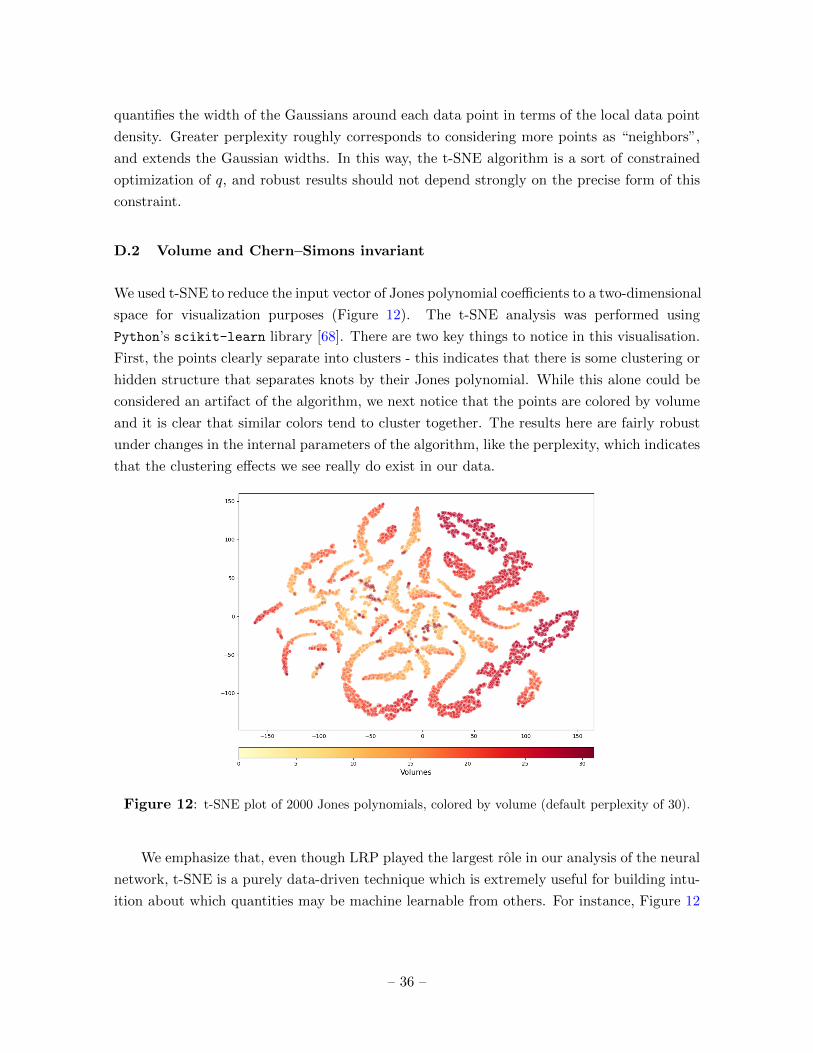
quantifies the width of the Gaussians around each data point in terms of the local data point

density. Greater perplexity roughly corresponds to considering more points as “neighbors”,

and extends the Gaussian widths. In this way, the t-SNE algorithm is a sort of constrained

optimization of q, and robust results should not depend strongly on the precise form of this

constraint.

D.2 Volume and Chern–Simons invariant

We used t-SNE to reduce the input vector of Jones polynomial coefficients to a two-dimensional

space for visualization purposes (Figure 12). The t-SNE analysis was performed using

Python’s scikit-learn library [68]. There are two key things to notice in this visualisation.

First, the points clearly separate into clusters - this indicates that there is some clustering or

hidden structure that separates knots by their Jones polynomial. While this alone could be

considered an artifact of the algorithm, we next notice that the points are colored by volume

and it is clear that similar colors tend to cluster together. The results here are fairly robust

under changes in the internal parameters of the algorithm, like the perplexity, which indicates

that the clustering effects we see really do exist in our data.

Figure 12: t-SNE plot of 2000 Jones polynomials, colored by volume (default perplexity of 30).

We emphasize that, even though LRP played the largest role in our analysis of the neural

network, t-SNE is a purely data-driven technique which is extremely useful for building intu-

ition about which quantities may be machine learnable from others. For instance, Figure 12

– 36 –

Figure 13: t-SNE plot of 2000 Jones polynomials, colored by Chern–Simons invariant (default

perplexity of 30).

demonstrates noticeable clustering, while Figure 13 does not. This is evidence that the hyper-

bolic volume may be machine learnable from the Jones polynomials, while the Chern–Simons

invariant may not be. Indeed, this intuition is confirmed in our experiments: none of the

neural networks we employed in this work were able to reliably predict the Chern–Simons

invariant of a knot from its Jones polynomial.

As a more general lesson, through the creation of plots like Figures 12 and 13, we can

visualize data without any choice of learning framework. This technique may have promising

applications in other areas of experimental mathematics or physics-inspired data science where

machine learning sometimes involves prohibitively large computational resources. In those

cases, t-SNE could be used to quickly iterate through hypotheses about correlations in the

dataset without running a full learning algorithm.

E Other experiments

In this appendix, we state the results of a number of mathematical experiments. In applying

artificial intelligence to problems in theoretical physics and mathematics, there is no a priori

understanding of what features are machine learnable. The problems for which machine

learning provides a useful prediction are often discovered by trial and error. Having isolated

– 37 –

such an instance in connecting the Jones polynomial with the hyperbolic volume, we believe

it is useful to publicize variations on this central theme.

We as well note some of the less successful experiments among our investigations. When

reverse engineering a neural network to obtain analytic results, we expect failed experiments

to also guide us. As reported in [16] and in Appendix D.2, the fact that the volume of the knot

complement and the Chern–Simons invariant appear on an equal footing in the generalized

volume conjecture (C.11) but only the former is machine learnable from J2(K; q) using a

simple neural network architecture is particularly striking and perhaps worth highlighting

again. It should also be noted that using evaluations of J2(K; q) at complex phases, we were

unable to predict the Chern–Simons invariant.

E.1 The HOMFLY-PT and Khovanov polynomials

The HOMFLY-PT polynomial P (K; a, z) [69, 70] is a two variable knot invariant that gen-

eralizes both the Alexander polynomial ∆(K; q) [71] and the Jones polynomial J2(K; q). In

particular,

∆(K; q) = P (K; 1, q1/2 − q−1/2) , J2(K; q) = P (K; q−1, q1/2 − q−1/2) . (E.1)

We have seen in Appendix B.1 that the Khovanov polynomial Kh(K; t, q) [58, 59] is another

such two variable polynomial invariant with the property that

J2(K; q2) =Kh(K;−1, q)

q + q−1. (E.2)

Using a similar architecture to what is quoted in Appendix A, we machine learn the volume

from the HOMFLY-PT polynomial to an accuracy of 93.9% from the full dataset of knots

up to 15 crossings. The Khovanov polynomial predicts the volume of the knot complement

to an accuracy of 97.2% from a partial dataset of 196, 002 knots up to 15 crossings. In both

experiments, we use 10% of the dataset for training. The input is a flattened matrix of

coefficients appearing in the polynomials where the dimensions of the matrix are determined

by the difference between the maximum and minimum degrees of the polynomials in each

of the two variables. We notice that though the HOMFLY-PT polynomial contains more

information about the knot than the Jones polynomial, it performs significantly worse when

used as the input in a two hidden layer neural network.

E.2 Representations of J2(K; q)

In [16], the Jones polynomial was faithfully represented as a vector. The first two terms of the

input vector are the minimum and maximum degree of the polynomial, and the subsequent

– 38 –

entries are the coefficients in the polynomial, padded to the right with zeros to form an

18-vector for knots up to 15 crossings and a 19-vector for knots up to 16 crossings. If we

represent the Jones polynomial, again faithfully, as a sparse vector in a long representation

whose length is determined by the difference between the maximum and minimum degrees of

all polynomials in the dataset, the performance is unchanged.

Surprisingly, unfaithful representations of the Jones polynomial perform almost as well.

If we eliminate the degrees from the vector and simply train on the coefficients (that is to

say, dimensions of particular Khovonov homology groups that differ for the various inputs),

the mean absolute error increases only slightly, from 2.65% to 2.75%. If the input vector

sorts the coefficients from smallest to largest, the results remain largely unchanged, but if

the ordering of the elements in each vector is randomized, then the mean absolute error is

6.44%, a significant loss of accuracy. While the ordering of the coefficients does matter (or

else the randomized vectors would perform just as well), the sorted vectors provide reasonable

accuracy, so some rearrangements are allowed. Linear combinations of the coefficients also

give an error less than 3%.

Let us drop the degrees but preserve the ordering of coefficients. This yields 16-vector

inputs for knots up to 15 crossings. In Appendix D, t-SNE was used to reduce the data to

two dimensions for visualization purposes: it allowed us to see the clustering of the inputs

according to volumes. Dimensional reduction may also be useful in determining how the

neural network learns the volume. Principal component analysis (PCA) is used as a method

to reduce the dimension of the data (length 16 to length 4). With this reduced input, the

error grows to 2.80%.

Extending Dunfield’s initial observation [14] that for alternating knots log |J2(K;−1)| ∝Vol(S3 \K), we consider the Taylor expansion of J2(K; eiπ(1−x)). For instance, for the figure-

eight knot 41, we have

J2(41; q) = q−2 − q−1 + 1− q + q2 , (E.3)

J2(41; eiπ(1−x)) = 5− 10π2

2!x2 +

34π4

4!x4 + . . . . (E.4)

We adopt the convention of dropping factors of i and π and write the first five coefficients as

a vector; this is (5, 0,−5, 0, 1.417) in the example 41. Using a dataset of 10, 000 alternating

knots between 11 and 15 crossings, the error in the neural network prediction of the volume

was 6.5%, and the performance was particularly poor at low volumes. Interesting, training

on the first coefficient alone, i.e., training on just J2(K;−1) yields superior performance.

– 39 –

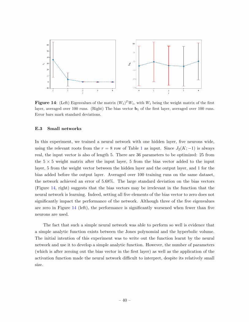
Figure 14: (Left) Eigenvalues of the matrix (W1)TW1, with W1 being the weight matrix of the first

layer, averaged over 100 runs. (Right) The bias vector b1 of the first layer, averaged over 100 runs.

Error bars mark standard deviations.

E.3 Small networks

In this experiment, we trained a neural network with one hidden layer, five neurons wide,

using the relevant roots from the r = 8 row of Table 1 as input. Since J2(K;−1) is always

real, the input vector is also of length 5. There are 36 parameters to be optimized: 25 from

the 5 × 5 weight matrix after the input layer, 5 from the bias vector added to the input

layer, 5 from the weight vector between the hidden layer and the output layer, and 1 for the

bias added before the output layer. Averaged over 100 training runs on the same dataset,

the network achieved an error of 5.68%. The large standard deviation on the bias vectors

(Figure 14, right) suggests that the bias vectors may be irrelevant in the function that the

neural network is learning. Indeed, setting all five elements of the bias vector to zero does not

significantly impact the performance of the network. Although three of the five eigenvalues

are zero in Figure 14 (left), the performance is significantly worsened when fewer than five

neurons are used.

The fact that such a simple neural network was able to perform so well is evidence that

a simple analytic function exists between the Jones polynomial and the hyperbolic volume.

The initial intention of this experiment was to write out the function learnt by the neural

network and use it to develop a simple analytic function. However, the number of parameters

(which is after zeroing out the bias vector in the first layer) as well as the application of the

activation function made the neural network difficult to interpret, despite its relatively small

size.

– 40 –

E.4 Symbolic regression

In [72], a combination of deep learning and symbolic regression is used to discover analytic

expressions. A deep learning model, such as a Graph Neural Network, is trained on available

data. Symbolic expressions are then fitted to the functions learned by the model. The software

PySR [73] automates this process. We used PySR to look for functions of the form V (K) =

f(|J2(K; e3πi/4)|), allowing the search to use all functions provided in the package. The best

fit predicts the volumes to 96.56% accuracy. While the precise formula is unenlightening, it

does include a logarithm of J2(K; e3πi/4), which reassures us that the formulas proposed in

Section 4 are reasonable ansatze.

References

[1] L. J. Dixon, Some worldsheet properties of superstring compactifications, on orbifolds and

otherwise, in Summer Workshop in High-energy Physics and Cosmology, 10, 1987.

[2] W. Lerche, C. Vafa and N. P. Warner, Chiral Rings in N=2 Superconformal Theories, Nucl.

Phys. B 324 (1989) 427–474.

[3] P. Candelas, M. Lynker and R. Schimmrigk, Calabi-Yau Manifolds in Weighted P(4), Nucl.

Phys. B 341 (1990) 383–402.

[4] B. R. Greene and M. Plesser, Duality in {Calabi-Yau} Moduli Space, Nucl. Phys. B 338 (1990)

15–37.

[5] P. Candelas, X. C. De La Ossa, P. S. Green and L. Parkes, A Pair of Calabi-Yau manifolds as

an exactly soluble superconformal theory, AMS/IP Stud. Adv. Math. 9 (1998) 31–95.

[6] A. Givental, Topological field theory, primitive forms and related topics, ch. A mirror theorem

for toric complete intersections, pp. 141–175. Springer, 1998.

[7] B. Lian, K. Liu and S.-T. Yau, Mirror principle. 1., Asian J. Math. 1 (1997) 729–763.

[8] V. F. R. Jones, Hecke algebra representations of braid groups and link polynomials, The Annals

of Mathematics 126 (Sep, 1987) 335.

[9] W. Thurston, The Geometry and Topology of 3-Manifolds, Lecture Notes, Princeton University

(1978) .

[10] E. Witten, Quantum Field Theory and the Jones Polynomial, Commun. Math. Phys. 121

(1989) 351–399.

[11] R. M. Kashaev, The hyperbolic volume of knots from quantum dilogarithm, Letters in

Mathematical Physics 39 (1997) 269–275, [arXiv:q-alg/9601025].

[12] H. Murakami and J. Murakami, The colored Jones polynomials and the simplicial volume of a

knot, Acta Math. 186 (2001) 85–104, [arXiv:math/9905075].

– 41 –

[13] S. Gukov, Three-dimensional quantum gravity, Chern-Simons theory, and the A polynomial,

Commun. Math. Phys. 255 (2005) 577–627, [hep-th/0306165].

[14] N. Dunfield, An interesting relationship between the Jones polynomial and hyperbolic volume,

Online (2000) .

[15] S. Garoufalidis and Y. Lan, Experimental evidence for the volume conjecture for the simplest

hyperbolic non-2–bridge knot, Algebraic & Geometric Topology 5 (May, 2005) 379–403,

[math/0412331].

[16] V. Jejjala, A. Kar and O. Parrikar, Deep Learning the Hyperbolic Volume of a Knot, Phys. Lett.

B 799 (2019) 135033, [1902.05547].

[17] L. G. Valiant, A theory of the learnable, Commun. ACM 27 (1984) 1134–1142.

[18] E. Witten, Analytic Continuation Of Chern-Simons Theory, AMS/IP Stud. Adv. Math. 50

(2011) 347–446, [1001.2933].

[19] W. P. Thurston, Three-Dimensional Geometry and Topology. Princeton University Press, 1997.

[20] V. Balasubramanian, J. R. Fliss, R. G. Leigh and O. Parrikar, Multi-Boundary Entanglement in

Chern-Simons Theory and Link Invariants, JHEP 04 (2017) 061, [1611.05460].

[21] V. Balasubramanian, M. DeCross, J. Fliss, A. Kar, R. G. Leigh and O. Parrikar, Entanglement

Entropy and the Colored Jones Polynomial, JHEP 05 (2018) 038, [1801.01131].

[22] T. Dimofte and S. Gukov, Quantum Field Theory and the Volume Conjecture, Contemp. Math.

541 (2011) 41–67, [1003.4808].

[23] Y. LeCun, Y. Bengio and G. Hinton, Deep learning, Nature 521 (May, 2015) 436–444.

[24] M. C. Hughes, A neural network approach to predicting and computing knot invariants,

1610.05744.

[25] S. Gukov, J. Halverson, F. Ruehle and P. Su lkowski, Learning to Unknot, 2010.16263.

[26] G. Cybenko, Approximation by superpositions of a sigmoidal function, Mathematics of Control,

Signals and Systems 2 (Dec, 1989) 303–314.

[27] K. Hornik, Approximation capabilities of multilayer feedforward networks, Neural networks 4

(1991) 251–257.

[28] J. Hoste, M. Thistlethwaite and J. Weeks, The first 1,701,936 knots, The Mathematical

Intelligencer 20 (1998) 33–48.

[29] “The knot atlas: The take home database.”

http://katlas.org/wiki/The_Take_Home_Database.

[30] M. Culler, N. M. Dunfield, M. Goerner and J. R. Weeks, “SnapPy, a computer program for

studying the geometry and topology of 3-manifolds.” http://snappy.computop.org.

[31] S. Bach, A. Binder, G. Montavon, F. Klauschen, K.-R. Muller and W. Samek, On pixel-wise

explanations for non-linear classifier decisions by layer-wise relevance propagation, PloS one 10

(2015) e0130140.

– 42 –

[32] G. Montavon, A. Binder, S. Lapuschkin, W. Samek and K.-R. Muller, Layer-wise relevance

propagation: an overview, in Explainable AI: interpreting, explaining and visualizing deep

learning, pp. 193–209. Springer, 2019.

[33] O. Dasbach and X.-S. Lin, A volumish theorem for the jones polynomial of alternating knots,

Pacific Journal of Mathematics 231 (Jun, 2007) 279–291.

[34] S.-M. Udrescu and M. Tegmark, AI Feynman: a Physics-Inspired Method for Symbolic

Regression, 1905.11481.

[35] S. Blucher, L. Kades, J. M. Pawlowski, N. Strodthoff and J. M. Urban, Towards novel insights

in lattice field theory with explainable machine learning, Phys. Rev. D 101 (2020) 094507,

[2003.01504].

[36] J. S. Cotler, G. Gur-Ari, M. Hanada, J. Polchinski, P. Saad, S. H. Shenker et al., Black Holes

and Random Matrices, JHEP 05 (2017) 118, [1611.04650].

[37] G. W. Moore, Introduction to chern–simons theories, Online (2019) .

[38] M. Khovanov, Patterns in knot cohomology, i, Experiment. Math. 12 (2003) 365–374.

[39] K. Habiro, On the colored jones polynomials of some simple links, Surikaisekikenkyusho

Kokyuroku (2000) 34–43.

[40] D. Bar-Natan, The symbol font dbnsymb, Online (2020) .

[41] M. Abadi, A. Agarwal, P. Barham, E. Brevdo, Z. Chen, C. Citro et al., TensorFlow: Large-scale

machine learning on heterogeneous systems, 2015.

[42] Y.-H. He, Deep-Learning the Landscape, 1706.02714.

[43] F. Ruehle, Evolving neural networks with genetic algorithms to study the String Landscape,

JHEP 08 (2017) 038, [1706.07024].

[44] D. Krefl and R.-K. Seong, Machine Learning of Calabi-Yau Volumes, Phys. Rev. D 96 (2017)

066014, [1706.03346].

[45] J. Carifio, J. Halverson, D. Krioukov and B. D. Nelson, Machine Learning in the String

Landscape, JHEP 09 (2017) 157, [1707.00655].

[46] K. Bull, Y.-H. He, V. Jejjala and C. Mishra, Machine Learning CICY Threefolds, Phys. Lett. B

785 (2018) 65–72, [1806.03121].

[47] K. Bull, Y.-H. He, V. Jejjala and C. Mishra, Getting CICY High, Phys. Lett. B 795 (2019)

700–706, [1903.03113].

[48] Y.-H. He and S.-T. Yau, Graph Laplacians, Riemannian Manifolds and their Machine-Learning,

2006.16619.

[49] Y.-H. He and A. Lukas, Machine Learning Calabi-Yau Four-folds, 2009.02544.

[50] J. Halverson, B. Nelson and F. Ruehle, Branes with Brains: Exploring String Vacua with Deep

Reinforcement Learning, JHEP 06 (2019) 003, [1903.11616].

– 43 –

[51] J. Halverson, M. Plesser, F. Ruehle and J. Tian, Kahler Moduli Stabilization and the

Propagation of Decidability, Phys. Rev. D 101 (2020) 046010, [1911.07835].

[52] J. Halverson and C. Long, Statistical Predictions in String Theory and Deep Generative Models,

Fortsch. Phys. 68 (2020) 2000005, [2001.00555].

[53] M. Bies, M. Cvetic, R. Donagi, L. Lin, M. Liu and F. Ruehle, Machine Learning and Algebraic

Approaches towards Complete Matter Spectra in 4d F-theory, 2007.00009.

[54] F. Ruehle, Data science applications to string theory, Physics Reports 839 (2020) 1 – 117.

[55] C. R. Brodie, A. Constantin, R. Deen and A. Lukas, Machine Learning Line Bundle

Cohomology, Fortsch. Phys. 68 (2020) 1900087, [1906.08730].

[56] C. R. Brodie, A. Constantin, R. Deen and A. Lukas, Topological Formulae for the Zeroth

Cohomology of Line Bundles on Surfaces, 1906.08363.

[57] C. R. Brodie, A. Constantin, R. Deen and A. Lukas, Index Formulae for Line Bundle

Cohomology on Complex Surfaces, Fortsch. Phys. 68 (2020) 1900086, [1906.08769].

[58] M. Khovanov, A categorification of the jones polynomial, Duke Math. J. 101 (02, 2000) 359–426.

[59] D. Bar-Natan, On khovanov’s categorification of the jones polynomial, Algebraic & Geometric

Topology 2 (May, 2002) 337–370, [math/0201043].

[60] L. H. Kauffman, State models and the jones polynomial, Topology 26 (1987) 395 – 407.

[61] K. P. Walsh, Patterns and Stability in the Coefficients of the Colored Jones Polynomial. PhD

thesis, UC, San Diego, 2014.

[62] K. P. Walsh, Higher order stability in the coefficients of the colored jones polynomial, Journal of

Knot Theory and Its Ramifications 27 (2018) 1840010, [1603.06957].

[63] T. T. Le, “The colored jones polynomial and the aj conjecture.”

http://people.math.gatech.edu/~letu/Papers/Lectures_Luminy_2014_new.pdf.

[64] V. F. Jones, “The jones polynomial for dummies.”

https://math.berkeley.edu/~vfr/jonesakl.pdf.

[65] V. F. Jones, “The jones polynomial.” https://math.berkeley.edu/~vfr/jones.pdf.

[66] H. Murakami, J. Murakami, M. Okamoto, T. Takata and Y. Yokota, Kashaev’s conjecture and

the chern-simons invariants of knots and links, Experimental Mathematics 11 (2002) 427–435.

[67] L. van der Maaten and G. Hinton, Visualizing data using t-SNE, Journal of Machine Learning

Research 9 (2008) 2579–2605.

[68] F. Pedregosa, G. Varoquaux, A. Gramfort, V. Michel, B. Thirion, O. Grisel et al., Scikit-learn:

Machine learning in Python, Journal of Machine Learning Research 12 (2011) 2825–2830.

[69] P. Freyd, D. Yetter, J. Hoste, W. B. R. Lickorish, K. Millett and A. Ocneanu, A new

polynomial invariant of knots and links, Bull. Am. Math. Soc. 12 (1985) 239–246.

[70] J. H. Przytycki and P. Traczyk, Conway algebras and skein equivalence of links, Proceedings of

the American Mathematical Society 100 (1987) 744–748.

– 44 –

[71] J. W. Alexander, Topological invariants of knots and links, Transactions of the American

Mathematical Society 30 (1928) 275–306.

[72] M. Cranmer, A. Sanchez-Gonzalez, P. Battaglia, R. Xu, K. Cranmer, D. Spergel et al.,

Discovering symbolic models from deep learning with inductive biases, NeurIPS 2020 (2020) ,

[2006.11287].

[73] M. Cranmer, Pysr: Fast & parallelized symbolic regression in python/julia, Sept., 2020.

10.5281/zenodo.4052869.

– 45 –