DISCLAIMER - ARM
22
Transcript of DISCLAIMER - ARM
DISCLAIMER
This report was prepared as an account of work sponsored by the U.S. Government. Neither the United States nor any agency thereof, nor any of their employees, makes any warranty, express or implied, or assumes any legal liability or responsibility for the accuracy, completeness, or usefulness of any information, apparatus, product, or process disclosed, or represents that its use would not infringe privately owned rights. Reference herein to any specific commercial product, process, or service by trade name, trademark, manufacturer, or otherwise, does not necessarily constitute or imply its endorsement, recommendation, or favoring by the U.S. Government or any agency thereof. The views and opinions of authors expressed herein do not necessarily state or reflect those of the U.S. Government or any agency thereof.
DOE/SC-ARM/TR-056
Cimel Sunphotometer (CSPHOT) Handbook L Gregory January 2011 Work supported by the U.S. Department of Energy, Office of Science, Office of Biological and Environmental Research

L Gregory, January 2011, DOE/SC-ARM/TR-056
ii
Contents
1.0 General Overview ................................................................................................................................. 1
2.0 Contacts ................................................................................................................................................ 1
2.1 Mentor .......................................................................................................................................... 1
2.2 Instrument Calibration and Data Processing ................................................................................ 2
2.3 Instrument Vendor........................................................................................................................ 2
3.0 Deployment Locations and History ...................................................................................................... 2
4.0 Near-Real-Time Data Plots .................................................................................................................. 3
5.0 Data Description and Examples ........................................................................................................... 4
5.1 Data File Contents ........................................................................................................................ 4
5.1.1 Primary Variables .............................................................................................................. 4
5.1.2 Measurement Accuracy ..................................................................................................... 4
5.2 Annotated Examples .................................................................................................................... 5
5.3 User Notes and Known Problems ................................................................................................ 7
5.3.1 Cloud Mode Zenith Radiance Data ................................................................................... 7
5.3.2 Data processing and Availability ...................................................................................... 8
5.4 Frequently Asked Questions ........................................................................................................ 8
6.0 Data Quality .......................................................................................................................................... 8
6.1 Data Quality Health and Status .................................................................................................... 8
6.2 Data Reviews by Instrument Mentor............................................................................................ 8
6.3 Data Assessments by Site Scientist/Data Quality Office ............................................................. 9
6.4 Value-Added Products and Quality Measurement Experiments .................................................. 9
7.0 Instrument Details............................................................................................................................... 10
7.1 Detailed Description ................................................................................................................... 10
7.1.1 List of Components ......................................................................................................... 10
7.1.2 System Configuration and Measurement Methods ......................................................... 10
7.1.3 Specifications .................................................................................................................. 13
7.2 Theory of Operation ................................................................................................................... 13
7.3 Calibration .................................................................................................................................. 14
7.3.1 Theory ............................................................................................................................. 14
7.3.2 Calibration Procedures .................................................................................................... 15
7.3.3 History ............................................................................................................................. 15
7.4 Operation and Maintenance ....................................................................................................... 15
7.4.1 User Manual .................................................................................................................... 15
7.4.2 Routine and Corrective Maintenance Documentation .................................................... 15
7.4.3 Software Documentation ................................................................................................. 16
7.4.4 Additional Documentation .............................................................................................. 16

L Gregory, January 2011, DOE/SC-ARM/TR-056
iii
7.5 Glossary ...................................................................................................................................... 16
7.6 Acronyms ................................................................................................................................... 16
7.7 Citable References...................................................................................................................... 17
Figures
1 Availability of ARM CSPHOT data. .................................................................................................... 32 AOT as a function of time. ................................................................................................................... 63 PW as a function of time. ...................................................................................................................... 64 Results of almucantar scan, size distribution derived from almucantar data using Nakajima’s
method, and phase function derived from the size distribution. ........................................................... 75 Schematic of CSPHOT systems and mounting configuration. ........................................................... 116 CSPHOT instrument parts and operation. .......................................................................................... 11
Tables
1 Instrument characteristics and observational specifications. .............................................................. 13

L Gregory, January 2011, DOE/SC-ARM/TR-056
1
1.0 General Overview
The Cimel sunphotometer (CSPHOT) is a multi-channel, automatic sun-and-sky scanning radiometer that measures the direct solar irradiance and sky radiance at the Earth’s surface. Measurements are taken at pre-determined discrete wavelengths in the visible and near-IR parts of the spectrum to determine atmospheric transmission and scattering properties. This instrument is weather-proof and requires little maintenance during periods of adverse weather conditions. It takes measurements only during daylight hours (sun above horizon).
2.0 Contacts
2.1 Mentor
Primary Contact for DQ and Instrument Coordination:
Laurie Gregory Brookhaven National Laboratory Environmental Science Dept., Bldg. 490D Upton, NY 11973-5000 Phone: +1-631-344-2266 E-mail: [email protected]
Principal Investigator (Science Questions):
Richard Wagener Brookhaven National Laboratory Environmental Science Dept., Bldg. 490D Upton, NY 11973-5000 Phone: +1-631-344-5886 E-mail: [email protected]
Instrument Hardware for ARM-Owned Systems:
Mark Klassen SGP Cart Site Operations Phone: +1-580-388-4053 E-mail: [email protected]
L Gregory, January 2011, DOE/SC-ARM/TR-056
2
2.2 Instrument Calibration and Data Processing
Aerosol Robotic Network (AERONET)
AERONET Aerosol Robotic Network NASA Goddard Space Flight Center Greenbelt, MD 20771 USA http://aeronet.gsfc.nasa.gov/
XDC Operations: Data Monitoring/Availability
Lynn Ma Brookhaven National Laboratory Environmental Science Dept., Bldg. 490D Upton, NY 11973-5000 Phone: +1-631-344-3813 E-mail: [email protected]
2.3 Instrument Vendor
CIMEL Electronique 172 rue de Charonne 75011 PARIS - France Phone: +33-1-43 48 79 33 http://www.cimel.fr/
3.0 Deployment Locations and History
As of January 2011, ARM owns and operates seven CSPHOTs in the field, one at each of the following sites:
• Southern Great Plains (SGP) C1
• Tropical Western Pacific (TWP) C1 (Manus)
• TWP C2 (Nauru)
• TWP C3 (Darwin)
• North Slope of Alaska (NSA) C1 (Barrow)
• ARM Mobile Facility 1 (AMF1)
• ARM Mobile Facility 2 (AMF2).

L Gregory, January 2011, DOE/SC-ARM/TR-056
3
A CSPHOT was first installed for long-term operations at the SGP site in March 1998. The NSA Barrow CSPHOT was installed in July 1997. The TWP Nauru CSPHOT was installed in June 1999. The TWP Darwin Cimel was installed in August 2010. The TWP Manus CSPHOT was installed in November, 2010.
The CSPHOT has also been deployed at the following AMF1 locations: Niamey, Niger (NIM) in 2006; Heselbach, Germany (FKB) in 2007; China (HFE) in 2008; and Graciosa Island, Azores (GRW) in 2009. With AMF2, the CSPHOT was deployed at Steamboat Springs (SBS) in 2010. AERONET also obtained data from a CSPHOT, owned by CSIRO, which was located at TWP C3 (Darwin) prior to the ARM CSPHOT installation.
ARM owns spare CSPHOTs that rotate to all sites except Barrow. This rotation is to swap out instruments that need to be returned to AERONET for post-deployment calibration, which typically takes several months. The NSA CSPHOT is calibrated during the winter months November through March.
Figure 1. Availability of ARM CSPHOT data.
4.0 Near-Real-Time Data Plots
Daily updated data plots for most sites can be found at AERONET: http://aeronet.gsfc.nasa.gov/.

L Gregory, January 2011, DOE/SC-ARM/TR-056
4
5.0 Data Description and Examples
5.1 Data File Contents
5.1.1 Primary Variables
The following is a list of the primary measurements for the CSPHOT:
• Aerosol absorption
• Aerosol concentration
• Aerosol extinction
• Aerosol optical properties
• Particle number concentration
• Particle size distribution
• Precipitable water
• Shortwave narrowband radiance
The data are supplied to the ARM Data Archive as external data and will have passed all quality checks. The issue of primary concern is the presence of clouds as the clouds may distort the data. Clouds are removed by inspection of triplet measurement in the level 1.5 (csphotaotfilt) data and by eliminating all data showing an Angstrom exponent of less than 0.5.
For a detailed listing of variables, see the data object designs of the various output datastreams:
• csphotalm: Cimel Sunphotometer (CSPHOT): almucantars sky radiance data
• csphotaot: Cimel Sunphotometer (CSPHOT): aerosol optical thickness data
• csphotaotfilt: Cimel Sunphotometer (CSPHOT): aerosol optical thickness, filtered data
• csphotaotqafilt: Cimel Sunphotometer (CSPHOT): aerosol optical thickness, filtered data
• csphotpp: Cimel Sunphotometer (CSPHOT): principal planes data
• csphotsize: Cimel Sunphotometer (CSPHOT): derived: aerosol size distributions
• csphottotalpfn1 (csphotpfn1): Cimel Sunphotometer (CSPHOT): almucantars sky radiance data, total mode. (Note: This is being changed to “csphotpfn1”, which includes total, fine, and coarse mode pfn data).
• csphotalm1dubo: Cimel Sunphotometer (CSPHOT) Dubovik almucantar retrievals
5.1.2 Measurement Accuracy
According to AERONET, the accuracy of the aerosol optical thickness is approximately 0.01–0.02 for field operated Cimels. Sky radiance measurements have an accuracy of +/- 5%. See the following excerpt from AERONET’s website for more details on how the accuracy is obtained:
The following is from: http://aeronet.gsfc.nasa.gov/new_web/system_descriptions_calibration.html

L Gregory, January 2011, DOE/SC-ARM/TR-056
5
“Direct Sun Calibration
Calibration refers to the determination of the calibration coefficients needed to convert the instrument output digital number (DN) to a desired output, in this case aerosol optical depth (AOD), precipitable water (cm), and radiance (W/m2/sr/um). Field instruments are generally returned to GSFC (Goddard Space Flight Center) for intercomparison with reference instruments approximately every 6 to 12 months in order to maintain accurate calibration. The GSFC reference Cimels are calibrated by the Langley technique at Mauna Loa Observatory in Hawaii on a frequent basis. The Langley Plot is a logarithm of the DN taken during these times plotted against the optical air mass between a range of 5 and 2 (between 3.5 and 2 for 340 nm), where the intercept is the calibration coefficient (zero air mass DN) and the slope is the optical depth. Langley plots from NOAA's Mauna Loa Observatory have been made to determine the spectral extraterrestrial voltage for these instruments since 1994. The observatory's high altitude and isolation from most local and regional sources of aerosols provides a very stable irradiance regime in the mornings, and is ideally suited to our purposes.
AERONET reference instruments are typically recalibrated at MLO every 2-3 months using the Langley plot technique. The zero air mass voltages [Vo, instrument voltage for direct normal solar flux extrapolated to the top of the atmosphere (Shaw, 1983)] are inferred to an accuracy of approximately 0.2 to 0.5% for the MLO calibrated reference instruments (Holben et al., 1998). Therefore the uncertainty in AOD due to the uncertainty in zero air mass voltages for the reference instruments is better than 0.002 to 0.005.
Radiance Calibration
For the sky radiance measurements, calibration is performed at the NASA Goddard Calibration Facility using a calibrated integrating sphere to an accuracy of +/- 5%. For the 940 nm channel that includes water absorption, calibration is performed using a variant of the modified Langley method. With respect to the long term stability of the calibration coefficients, the optical interference filters are the limiting factors. On average, there has been a decrease from 1 to 10% per year. Therefore, instruments are calibrated on a 6- to 12-month rotation and filters are changed when needed.
Interpolation and Uncertainty
The Sun-sky radiometers at sites other than GSFC are intercalibrated against a MLO calibrated AERONET reference instrument both before deployment in the field and post- deployment. A linear rate of change in time of the zero air mass voltages is then assumed in the processing of the data from field sites. Our analysis suggests that this results in an uncertainty of approximately 0.01 - 0.02 in AOD (wavelength dependent) due to calibration uncertainty for the field instruments.”
5.2 Annotated Examples
Current and recent data quicklooks – Go to Real Time Data (Level 1).
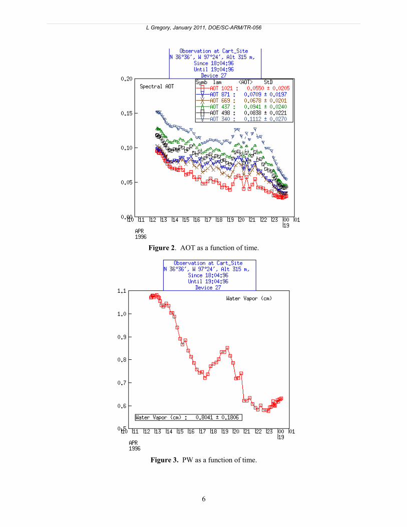
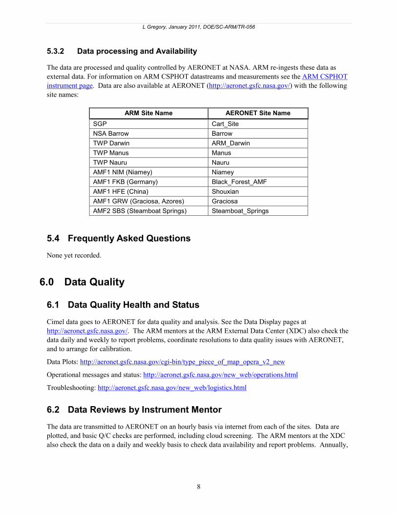
AOT and PW as a function of time are depicted in Figures 2 and 3 as a function of time for one day. Also shown in Figure 4 are results of almucantar scan, size distribution derived from almucantar data using Nakajima’s method (Nakajima et al. 1983), and phase function derived from the size distribution using the same method.
L Gregory, January 2011, DOE/SC-ARM/TR-056
6
Figure 2. AOT as a function of time.
Figure 3. PW as a function of time.

L Gregory, January 2011, DOE/SC-ARM/TR-056
7
Figure 4. Results of almucantar scan, size distribution derived from almucantar data using Nakajima’s
method (Nakajima et al. 1983), and phase function derived from the size distribution.
5.3 User Notes and Known Problems
5.3.1 Cloud Mode Zenith Radiance Data
In addition to normal operations, ARM has participated in the past few years in the development of cloud mode data from the Cimel Sunphotometers. This mode is used to measure zenith radiance when routine aerosol measurements are unable to be taken, i.e. overcast with non-precipitating clouds. With the participation of ARM scientists in developing algorithms for the method, AERONET has announced that the use of this mode would go operational in 2010. AERONET now has expanded the use of cloud mode to many of their sites in their worldwide network. ARM continues its participation by running all sites with cloud mode when environmental conditions allow for it, i.e. vegetated surface, no snow.
The zenith radiance during overcast conditions is used together with the surface reflectances at 440 nm and 870 nm from MODIS to derive cloud optical depth. Since the algorithm is still in a developmental stage, the provisional cloud optical depth data are currently only available at AERONET's website. To view the data, please see: http://aeronet.gsfc.nasa.gov/cgi-bin/type_piece_of_map_cloud.
L Gregory, January 2011, DOE/SC-ARM/TR-056
8
5.3.2 Data processing and Availability
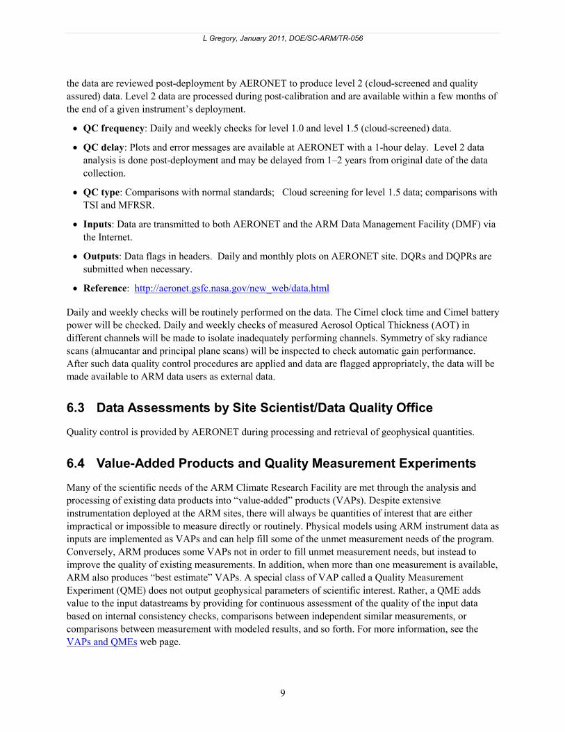
The data are processed and quality controlled by AERONET at NASA. ARM re-ingests these data as external data. For information on ARM CSPHOT datastreams and measurements see the ARM CSPHOT instrument page. Data are also available at AERONET (http://aeronet.gsfc.nasa.gov/) with the following site names:
ARM Site Name AERONET Site Name SGP Cart_Site NSA Barrow Barrow TWP Darwin ARM_Darwin TWP Manus Manus TWP Nauru Nauru AMF1 NIM (Niamey) Niamey AMF1 FKB (Germany) Black_Forest_AMF AMF1 HFE (China) Shouxian AMF1 GRW (Graciosa, Azores) Graciosa AMF2 SBS (Steamboat Springs) Steamboat_Springs
5.4 Frequently Asked Questions
None yet recorded.
6.0 Data Quality
6.1 Data Quality Health and Status
Cimel data goes to AERONET for data quality and analysis. See the Data Display pages at http://aeronet.gsfc.nasa.gov/. The ARM mentors at the ARM External Data Center (XDC) also check the data daily and weekly to report problems, coordinate resolutions to data quality issues with AERONET, and to arrange for calibration.
Data Plots: http://aeronet.gsfc.nasa.gov/cgi-bin/type_piece_of_map_opera_v2_new
Operational messages and status: http://aeronet.gsfc.nasa.gov/new_web/operations.html
Troubleshooting: http://aeronet.gsfc.nasa.gov/new_web/logistics.html
6.2 Data Reviews by Instrument Mentor
The data are transmitted to AERONET on an hourly basis via internet from each of the sites. Data are plotted, and basic Q/C checks are performed, including cloud screening. The ARM mentors at the XDC also check the data on a daily and weekly basis to check data availability and report problems. Annually,
L Gregory, January 2011, DOE/SC-ARM/TR-056
9
the data are reviewed post-deployment by AERONET to produce level 2 (cloud-screened and quality assured) data. Level 2 data are processed during post-calibration and are available within a few months of the end of a given instrument’s deployment.
• QC frequency: Daily and weekly checks for level 1.0 and level 1.5 (cloud-screened) data.
• QC delay: Plots and error messages are available at AERONET with a 1-hour delay. Level 2 data analysis is done post-deployment and may be delayed from 1–2 years from original date of the data collection.
• QC type: Comparisons with normal standards; Cloud screening for level 1.5 data; comparisons with TSI and MFRSR.
• Inputs: Data are transmitted to both AERONET and the ARM Data Management Facility (DMF) via the Internet.
• Outputs: Data flags in headers. Daily and monthly plots on AERONET site. DQRs and DQPRs are submitted when necessary.
• Reference: http://aeronet.gsfc.nasa.gov/new_web/data.html
Daily and weekly checks will be routinely performed on the data. The Cimel clock time and Cimel battery power will be checked. Daily and weekly checks of measured Aerosol Optical Thickness (AOT) in different channels will be made to isolate inadequately performing channels. Symmetry of sky radiance scans (almucantar and principal plane scans) will be inspected to check automatic gain performance. After such data quality control procedures are applied and data are flagged appropriately, the data will be made available to ARM data users as external data.
6.3 Data Assessments by Site Scientist/Data Quality Office
Quality control is provided by AERONET during processing and retrieval of geophysical quantities.
6.4 Value-Added Products and Quality Measurement Experiments
Many of the scientific needs of the ARM Climate Research Facility are met through the analysis and processing of existing data products into “value-added” products (VAPs). Despite extensive instrumentation deployed at the ARM sites, there will always be quantities of interest that are either impractical or impossible to measure directly or routinely. Physical models using ARM instrument data as inputs are implemented as VAPs and can help fill some of the unmet measurement needs of the program. Conversely, ARM produces some VAPs not in order to fill unmet measurement needs, but instead to improve the quality of existing measurements. In addition, when more than one measurement is available, ARM also produces “best estimate” VAPs. A special class of VAP called a Quality Measurement Experiment (QME) does not output geophysical parameters of scientific interest. Rather, a QME adds value to the input datastreams by providing for continuous assessment of the quality of the input data based on internal consistency checks, comparisons between independent similar measurements, or comparisons between measurement with modeled results, and so forth. For more information, see the VAPs and QMEs web page.

L Gregory, January 2011, DOE/SC-ARM/TR-056
10
For the CSPHOT, size distribution and phase function can be considered as value-added products. The AOT comparison with MFRSR-derived values and the PW comparison with radiosonde and microwave radiometer values are QMEs.
7.0 Instrument Details
7.1 Detailed Description
7.1.1 List of Components
The CSPHOT consists of (1) the instrument itself (made up of the sensor head and scanning motors and robot arm); (2) a control box (provides software for controlling predetermined scanning and sampling strategies, and for acquiring data.); and (3) a computer for data collection and transmission. The instrument is made by Cimel Electronique of France.
Until 2006, a GOES satellite transmitter was used to transmit data to AERONET. Since 2006, however, data transfer has been switched to network-based transmissions.
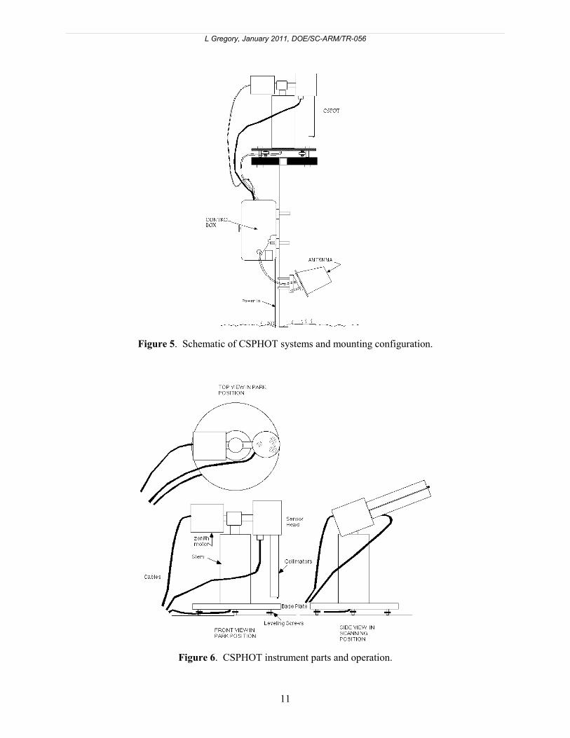
Figure 5 presents a schematic of a CSPHOT in a mounted configuration. This figure shows the Antenna for the GOES transmitter. However, this is no longer required.
7.1.2 System Configuration and Measurement Methods
The following paragraphs describe the components that make up the system (see Figure 6). More information can be found on AERONET’s page at: http://aeronet.gsfc.nasa.gov/new_web/system_descriptions.html
7.1.2.1 Instrument
The instrument consists of the main stem containing the azimuth motor. On the top of the motor is an attached robot arm consisting of the zenith motor on one side and the sensor head on the other side. The collimators are attached to the sensor head. Inside the sensor head are two silicon detectors, one for each of the collimators. A filter wheel is placed in between the collimator windows and the detectors, inside the sensor head. The wheel consists of eight narrowband interference filters (at 340, 380, 440, 500, 675, 870, 1020, and 1640 nm) mounted along the circumference. The two collimators have the same field of view (1.2 degree) but differ in the size of apertures. They are physically part of a single unit that is attached to the sensor head by a long screw tightened down to prevent light and water leakage. The larger aperture collimator—10 times as large as the sun-viewing collimator—provides the necessary dynamic range to observe the sky. Three cables (a thick cable from the sensor head to the control box, and two battery power cables—one each to the motors) are attached to the instrument. The main stem is connected to a base plate consisting of mounting holes to ensure the instrument is mounted on a level surface.
L Gregory, January 2011, DOE/SC-ARM/TR-056
11
Figure 5. Schematic of CSPHOT systems and mounting configuration.
Figure 6. CSPHOT instrument parts and operation.

L Gregory, January 2011, DOE/SC-ARM/TR-056
12
7.1.2.2 Control Boxes
The Cimel control box consists of a control module—a rectangular white box—that actually controls the scan and measurement sequence of CSPHOT. It has an internal battery that services only the software portion of the instrument. The box also stores data that can be queried and is transferred to the instrument computer. The control box also includes a battery pack that supplies power to the CSPHOT control box. A separate battery charger provides the necessary power from the input mains.
7.1.2.3 Location (Siting)
The instrument is located at a height of about five feet from the surface to minimize accidental obstruction of the field of view of the collimators. The location should allow an unobstructed view of the sky above five degrees of elevation, especially in the general region of sunset and sunrise at the ARM sites.
7.1.2.4 Weather-Related Details
All of the cables interconnecting the above components pass through rainproof silicone seals in their respective boxes. A wet sensor, connected to the instrument control box, effectively shuts down the scanning by the sensor head during precipitation. The fail-safe pointing for the sensor head is the “down” position with the collimators pointing down toward the base. Note that the wet-sensor does not detect snow, so the instrument should not be operated in cloud mode during the snow season.
7.1.2.5 Measurement Method
CSPHOT operates automatically without operator assistance. It measures direct solar irradiance by first pointing the collimator toward the approximate position of the sun (provided it is aligned properly) based on a built-in program that takes into account the time of the year and the coordinates of the location that are input to the Cimel control box prior to operation. A four-quadrant detector then positions the sun at the center of the fields of view of the collimators by using a feedback control loop. The filter wheel rotates in front of the detector to obtain a measurement sequence. A sequence takes about 10 seconds. In order to discriminate against the presence of thin cirrus clouds, which may be non-uniform, three measurement sequences are performed (called a triplet), lasting about 35 seconds. During a data analysis procedure, the measured voltages are compared to eliminate non-uniform scenes. Almucantar sky radiance is obtained by scanning the sky at the solar zenith angle but different azimuth angles to obtain the angular variation of skylight in four filters. Solar principal plane sky measurement is obtained by scanning the sky in a plane containing the sun and the instrument and normal to the surface. Data are taken more frequently near the sun since the intensity varies rapidly in the solar aureole. The sky brightness data are inverted by radiative transfer routines to derive aerosol size distribution and phase function.
For more information regarding the instrument operation see: http://aeronet.gsfc.nasa.gov/new_web/system_descriptions_operation.html.
As of 2007, cloud mode has been added to the ARM Cimel Sunphotometers to provide calibrated zenith radiances. As of June 2010, the cloud mode data are in development. However, they are planned to be incorporated operationally into the AERONET network in the near future.
L Gregory, January 2011, DOE/SC-ARM/TR-056
13
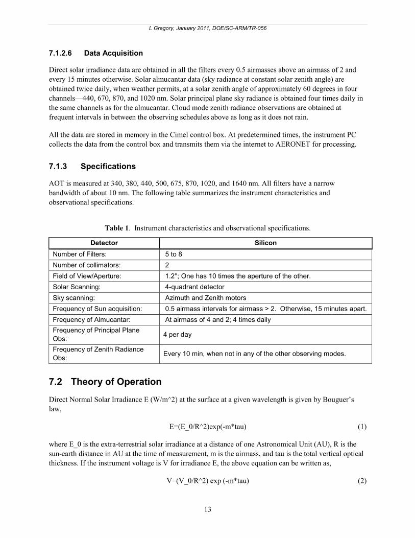
7.1.2.6 Data Acquisition
Direct solar irradiance data are obtained in all the filters every 0.5 airmasses above an airmass of 2 and every 15 minutes otherwise. Solar almucantar data (sky radiance at constant solar zenith angle) are obtained twice daily, when weather permits, at a solar zenith angle of approximately 60 degrees in four channels—440, 670, 870, and 1020 nm. Solar principal plane sky radiance is obtained four times daily in the same channels as for the almucantar. Cloud mode zenith radiance observations are obtained at frequent intervals in between the observing schedules above as long as it does not rain.
All the data are stored in memory in the Cimel control box. At predetermined times, the instrument PC collects the data from the control box and transmits them via the internet to AERONET for processing.
7.1.3 Specifications
AOT is measured at 340, 380, 440, 500, 675, 870, 1020, and 1640 nm. All filters have a narrow bandwidth of about 10 nm. The following table summarizes the instrument characteristics and observational specifications.
Table 1. Instrument characteristics and observational specifications.
Detector Silicon Number of Filters: 5 to 8 Number of collimators: 2 Field of View/Aperture: 1.2°; One has 10 times the aperture of the other. Solar Scanning: 4-quadrant detector Sky scanning: Azimuth and Zenith motors Frequency of Sun acquisition: 0.5 airmass intervals for airmass > 2. Otherwise, 15 minutes apart. Frequency of Almucantar: At airmass of 4 and 2; 4 times daily Frequency of Principal Plane Obs: 4 per day
Frequency of Zenith Radiance Obs: Every 10 min, when not in any of the other observing modes.
7.2 Theory of Operation
Direct Normal Solar Irradiance E (W/m^2) at the surface at a given wavelength is given by Bouguer’s law,
E=(E_0/R^2)exp(-m*tau) (1)
where E_0 is the extra-terrestrial solar irradiance at a distance of one Astronomical Unit (AU), R is the sun-earth distance in AU at the time of measurement, m is the airmass, and tau is the total vertical optical thickness. If the instrument voltage is V for irradiance E, the above equation can be written as,
V=(V_0/R^2) exp (-m*tau) (2)
L Gregory, January 2011, DOE/SC-ARM/TR-056
14
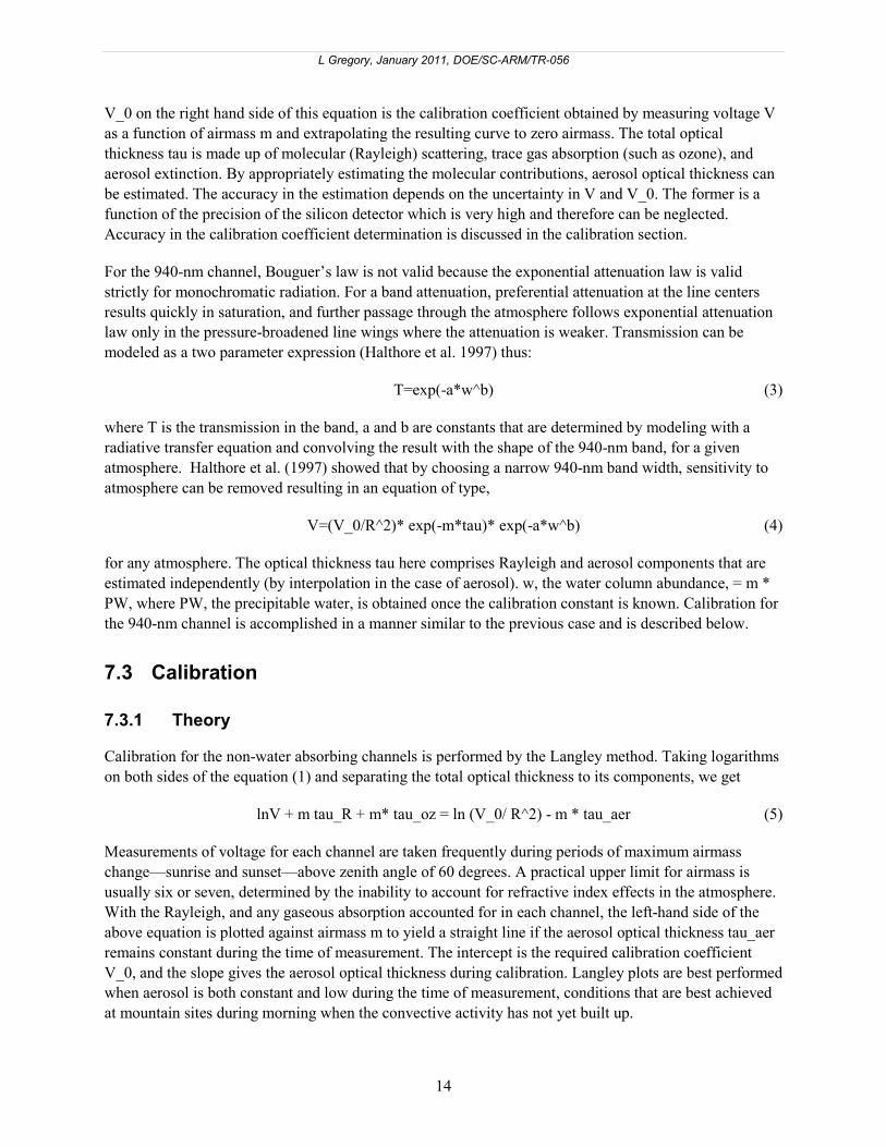
V_0 on the right hand side of this equation is the calibration coefficient obtained by measuring voltage V as a function of airmass m and extrapolating the resulting curve to zero airmass. The total optical thickness tau is made up of molecular (Rayleigh) scattering, trace gas absorption (such as ozone), and aerosol extinction. By appropriately estimating the molecular contributions, aerosol optical thickness can be estimated. The accuracy in the estimation depends on the uncertainty in V and V_0. The former is a function of the precision of the silicon detector which is very high and therefore can be neglected. Accuracy in the calibration coefficient determination is discussed in the calibration section.
For the 940-nm channel, Bouguer’s law is not valid because the exponential attenuation law is valid strictly for monochromatic radiation. For a band attenuation, preferential attenuation at the line centers results quickly in saturation, and further passage through the atmosphere follows exponential attenuation law only in the pressure-broadened line wings where the attenuation is weaker. Transmission can be modeled as a two parameter expression (Halthore et al. 1997) thus:
T=exp(-a*w^b) (3)
where T is the transmission in the band, a and b are constants that are determined by modeling with a radiative transfer equation and convolving the result with the shape of the 940-nm band, for a given atmosphere. Halthore et al. (1997) showed that by choosing a narrow 940-nm band width, sensitivity to atmosphere can be removed resulting in an equation of type,
V=(V_0/R^2)* exp(-m*tau)* exp(-a*w^b) (4)
for any atmosphere. The optical thickness tau here comprises Rayleigh and aerosol components that are estimated independently (by interpolation in the case of aerosol). w, the water column abundance, = m * PW, where PW, the precipitable water, is obtained once the calibration constant is known. Calibration for the 940-nm channel is accomplished in a manner similar to the previous case and is described below.
7.3 Calibration
7.3.1 Theory
Calibration for the non-water absorbing channels is performed by the Langley method. Taking logarithms on both sides of the equation (1) and separating the total optical thickness to its components, we get
lnV + m tau_R + m* tau_oz = ln (V_0/ R^2) - m * tau_aer (5)
Measurements of voltage for each channel are taken frequently during periods of maximum airmass change—sunrise and sunset—above zenith angle of 60 degrees. A practical upper limit for airmass is usually six or seven, determined by the inability to account for refractive index effects in the atmosphere. With the Rayleigh, and any gaseous absorption accounted for in each channel, the left-hand side of the above equation is plotted against airmass m to yield a straight line if the aerosol optical thickness tau_aer remains constant during the time of measurement. The intercept is the required calibration coefficient V_0, and the slope gives the aerosol optical thickness during calibration. Langley plots are best performed when aerosol is both constant and low during the time of measurement, conditions that are best achieved at mountain sites during morning when the convective activity has not yet built up.
L Gregory, January 2011, DOE/SC-ARM/TR-056
15
For the 940-nm channel, calibration is performed by the modified-Langley method. This is best illustrated by taking logarithms on both side of equation (2) to obtain
ln V + m* tau = ln (V_0 / R^2) - a * PW^b * m^b (6)
where the column abundance along the path, w, is written in terms of the product of the precipitable water, which is the water vapor vertical column abundance and airmass m. Thus, a plot of the left-hand side versus m^b will yield a straight line if, in addition to the aerosol optical thickness (contained in the ordinate), PW also remains constant. AOT is estimated for the 940-nm channel by interpolation between 870 and 1020 nm channels. Here a and b are constants that are determined (Halthore et al. 1997) by running a radiative transfer model such as MODTRAN-3 and convolving its output with the measured filter function of the 940-nm band. Narrow band widths yield values of a and b that are independent of the type of atmosphere present.
7.3.2 Calibration Procedures
Instruments are swapped out and sent to AERONET on an annual basis for calibration. For more information on calibration see Section 5.1.2 of this document describing measurement accuracy.
7.3.3 History
Any change in the calibration coefficients will be documented, and the calibration event and the method will be listed in one file that will be part of the database at AERONET. The calibration coefficients are linearly interpolated between pre- and post-deployment calibrations. Large changes in calibration coefficients between pre- and post-deployment will result in large uncertainties in the derived measurements. If the AERONET analyst deems the change too large the data will not be processed to the quality assured level 2.
7.4 Operation and Maintenance
7.4.1 User Manual • User manual from Cimel: http://www.cimel.fr/photo/pdf/man_ce318_us.pdf
• Setup manual from AERONET: http://aeronet.gsfc.nasa.gov/new_web/Documents/Cimel_set_up.pdf
• Additional information is available on AERONET’s website: http://aeronet.gsfc.nasa.gov/
7.4.2 Routine and Corrective Maintenance Documentation
Routine maintenance should be performed weekly, including checking battery connections, checking the wet sensor, checking the instrument clocks, and checking that robot and parked sensor head are level and that the collimator tubes are clear. For detailed and step-by-step instructions please see:
http://aeronet.gsfc.nasa.gov/new_web/checklist_english.html.

L Gregory, January 2011, DOE/SC-ARM/TR-056
16
Cloud mode setup and maintenance
Routine setup and maintenance should also include the setup and monitoring of cloud mode. When cloud mode is in operation, it is critical that the wet sensor is checked weekly to ensure that it is working properly and rain does not get into the collimator tubes. Cloud mode should be turned on at all sites upon installation, except during snow conditions. AERONET has suggested that cloud mode be turned off during snow conditions since the wet sensor may not detect snow and snow in the collimator tube risks the calibration accuracy.
Below is the sequence of buttons on the Cimel instrument control panels to turn cloud mode on:
• PW 1
• PAR
• Scroll down to BCL_SKY NO using the "x" button and change "NO" to "YES"
• Write / Save to EPROM
• EXIT
Note: Use the same sequence to turn cloud mode off, changing “YES” to “NO” for BCL_SKY.
7.4.3 Software Documentation
Starting in 2009, the data software was upgraded from ASTPWin software collection to using AERONET’s cimel connect program.
http://aeronet.gsfc.nasa.gov/new_web/Documents/AERONET_Cimel_Connect_HTTP.pdf
7.4.4 Additional Documentation
This section is not applicable to this instrument.
7.5 Glossary
See the ARM Glossary.
7.6 Acronyms
See the ARM Acronyms and Abbreviations.

L Gregory, January 2011, DOE/SC-ARM/TR-056
17
7.7 Citable References
Halthore, RN, TF Eck, BN Holben, and BL Markham. 1997. “Sunphotometric measurements of atmospheric water vapor column abundance in the 940-nm band. Journal of Geophysical Research 102: 4343–4352.
Holben, BN, TF Eck, I Slutsker, D Tanre, JP Buis, A Setzer, E Vermote, J Reagan, Y Kaufman, T Nakajima, F Lavenu, and I Jankowiak. 1997. “Automatic sun and sky scanning radiometer system for network aerosol monitoring.” Accepted for publication in Remote Sensing of Environment.
Nakajima, T, M Tanaka, and T Yamauchi. 1983. “Retrieval of the optical properties of aerosols from aureole and extinction data.” Applied Optics 22: 2951–2959.