Direct Methods for Sparse Matrices - avcr.cztuma/ps/direct.pdf1.c) Data structures for sparse...
87
Direct Methods for Sparse Matrices Miroslav T˚ uma Institute of Computer Science Academy of Sciences of the Czech Republic and Technical University in Liberec 1
Transcript of Direct Methods for Sparse Matrices - avcr.cztuma/ps/direct.pdf1.c) Data structures for sparse...

Direct Methods for SparseMatrices
Miroslav Tuma
Institute of Computer Science
Academy of Sciences of the Czech Republic
and
Technical University in Liberec
1

This is a lecture prepared for the SEMINAR ON NUMERICAL
ANALYSIS: Modelling and Simulation of Challenging Engineer-
ing Problems, held in Ostrava, February 7–11, 2005. Its purpose
is to serve as a first introduction into the field of direct methods
for sparse matrices. Therefore, it covers only the most classical
results of a part of the field, typically without citations. The
lecture is a first of the three parts which will be presented in
the future. The contents of subsequent parts is indicated in the
outline.
The presentation is partially supported by the project within the
National Program of Research “Information Society” under No.
1ET400300415
2

Outline
1. Part I.
2. Sparse matrices, their graphs, data structures
3. Direct methods
4. Fill-in in SPD matrices
5. Preprocessing for SPD matrices
6. Algorithmic improvements for SPD decompositions
7. Sparse direct methods for SPD matrices
8. Sparse direct methods for nonsymmetric matrices
3

Outline (continued)
1. Part II. (not covered here)
2. Fill-in in LU decomposition
3. Reorderings for LU decomposition
4. LU decompositions based on partial pivoting
5. LU decompositions based on full/relaxed pivoting
6. Part III. (not covered here)
7. Parallel sparse direct methods
8. Parallel SPD sparse direct methods
9. Parallel nonsymetric sparse direct methods
10. Sparse direct methods: sequential and parallel codes
4
1. Sparse matrices, their graphs, data structures
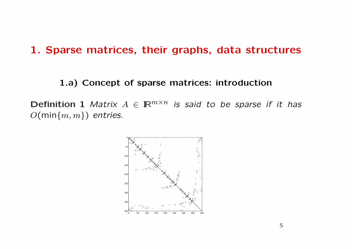
1.a) Concept of sparse matrices: introduction
Definition 1 Matrix A ∈ IRm×n is said to be sparse if it hasO(min{m, m}) entries.
0 50 100 150 200 250 300 350 400
0
50
100
150
200
250
300
350
400
5

1.a) Concept of sparse matrices: other definitions
Definition 2 Matrix A ∈ IRm×n is said to be sparse if it has row
counts bounded by rmax << n or column counts bounded by
cmax << n.
Definition 3 Matrix A ∈ IRm×n is said to be sparse if its number
of nonzero entries is O(n1+γ) for some γ < 1.
Definition 4 (pragmatic definition: J.H. Wilkinson) Matrix
A ∈ IRm×n is said to be sparse if we can exploit the fact that a
part of its entries is equal to zero.
6

1.a) Concept of sparse matrices: an example showing
importance of the small exponent γ for n = 104
γ n1+γ
0.1 251190.2 630960.3 1584890.4 3981070.5 1000000
7

1.b) Matrices and their graphs: introduction
Matrices, or their structures (i.e., positions of nonzero
entries) can be conveniently expressed by graphs
⇓
Different graph models for different purposes
• undirected graph
• directed graph
• bipartite graph
8

1.b) Matrices and their graphs: undirected graphs
Definition 5 A simple undirected graph is an ordered pair of
sets (V, E) such that E = {{i, j}|i ∈ V, j ∈ V }. V is called the
vertex (node) set and E is called the edge set.
9

1.b) Matrices and their graphs: directed graphs
Definition 6 A simple directed graph is an ordered pair of sets
(V, E) such that E = {(i, j)|i ∈ V, j ∈ V }. V is called the vertex
(node) set and E is called the edge (arc) set.
10

1.b) Matrices and their graphs: bipartite graphs
Definition 7 A simple bipartite graph is an ordered pair of sets
(R, C, E) such that E = {{i, j}|i ∈ R, j ∈ C}. R is called the row
vertex set, C is called the column vertex set and E is called
the edge set.
11

1.b) Matrices and their graphs: relation matrix → graph
Definition 8{x, y} ∈ E or (x, y) ∈ E ⇔ vertices x and y are adjacent
Adj(x) = {y|y and x are adjacent }
Structure of a nonsymmetric matrix and its graph
∗ ∗∗ ∗ ∗∗ ∗∗ ∗∗ ∗
∗ ∗ ∗
12
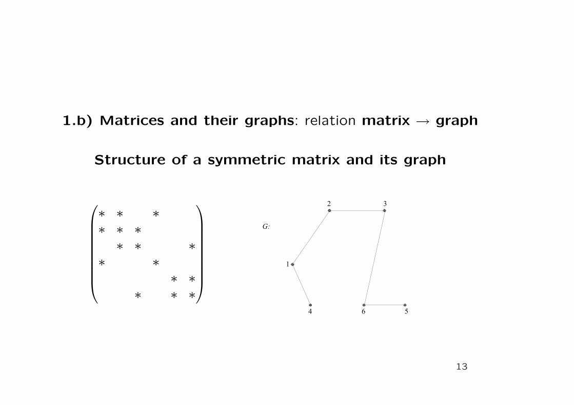
1.b) Matrices and their graphs: relation matrix → graph
Structure of a symmetric matrix and its graph
∗ ∗ ∗∗ ∗ ∗∗ ∗ ∗
∗ ∗∗ ∗
∗ ∗ ∗
13

1.c) Data structures for sparse matrices: sparse vectors
v =(3.1 0 2.8 0 0 5 4.3
)T
AV 3.12.8 5 4.3
JV 1 3 6 7
14

1.c) Data structures for sparse matrices: static data
structures
• static: difficult/costly entry insertion, deletion
• CSR (Compressed Sparse by Rows) format: stores matrix
rows as sparse vectors one after another
• CSC: analogical format by columns
• connection tables: 2D array with n rows and m colums
where m denotes maximum count of a row of the stored
matrix
• A lot of other general / specialized formats
15
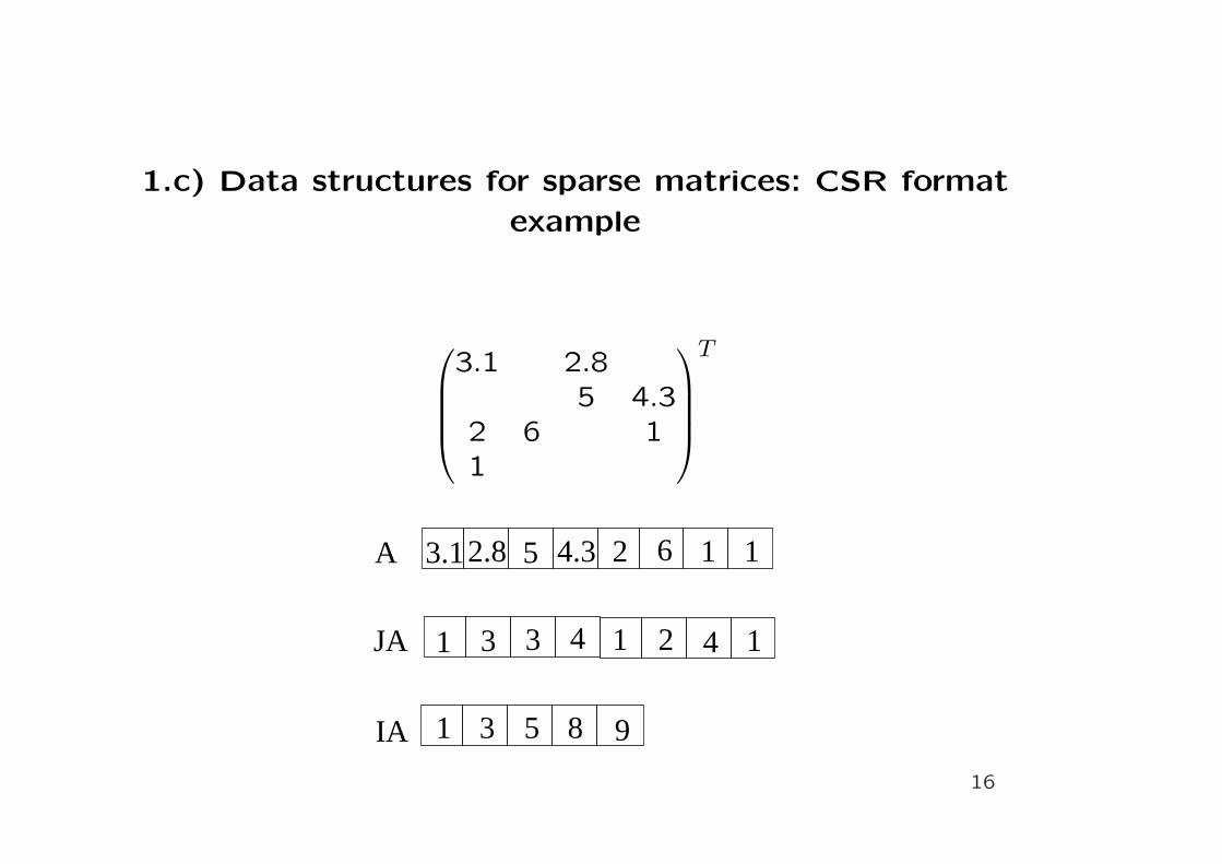
1.c) Data structures for sparse matrices: CSR format
example
3.1 2.85 4.3
2 6 11
T
3.12.8 5 4.3 2 6 1 1
1 1
1
3 3 4 2 4 1
3 5 8 9
A
JA
IA
16

1.c) Data structures for sparse matrices: dynamic data
structures
• dynamic: easy entry insertion, deletion
• linked list - based format: stores matrix rows/columns as
items connected by pointers
• linked lists can be cyclic, one-way, two-way
• rows/columns embedded into a larger array: emulated dy-
namic behavior
2 6 1
17

1.c) Data structures for sparse matrices: static versusdynamic data structures
• dynamic data structures:
• – more flexible but this flexibility might not be needed
• – difficult to vectorize
• – difficult to keep spatial locality
• – used preferably for storing vectors
• static data structures:
• – we need to avoid ad-hoc insertions/deletions
• – much simpler to vectorize
• – efficient access to rows/columns
18

2. Direct methods
2.a) Dense direct methods: introduction
• methods based on solving Ax = b by a matrix decomposition– variant of Gaussian elimination; typical decompositions:
• – A = LLT , A = LDLT (Cholesky decomposition, LDLT de-composition for SPD matrices)
• – A = LU (LU decomposition for general nonsymmetric ma-trices)
• – A = LBLT (symmetric indefinite / diagonal pivoting de-composition for A symmetric indefinite)
three steps of a (basic!) direct method:1) A → LU , 2) y from Ly = b, 3) x from Ux = y
19

2.a) Dense direct methods: elimination versus
decomposition
• Householder (end of 1950’s, beginning of 1960’s): expressing
Gaussian elimination as a decomposition
• Various reformulations of the same decomposition: different
properties in
• – sparse implementations
• – vector processing
• – parallel implementations
• We will show six basic algorithms but there are others (bor-
dering, Dongarra-Eisenstat)
20

Algorithm 1 ikj lu decomposition (delayed row dense algorithm)
l = In
u = On
u11:n = a1,1:n
for i=2:n
for k=1:i-1
lik = aik/akk
for j=k+1:n
aij = aij − lik ∗ akj
end
end
uii:n = aii:n
end
� � � � � � � � � � � � � � � � � � � � � � � � � � �� � � � � � � � � � � � � � � � � � � � � � � � � � �� � � � � � � � � � � � � � � � � � � � � � � � � � �� � � � � � � � � � � � � � � � � � � � � � � � � � �
i
21

Algorithm 2 ijk lu decomposition (dot product - based row
dense algorithm)
l = In, u = On, u11:n = a11:n
for i=2:n
for j=2:i
lij−1 = aij−1/aj−1j−1
for k=1:j-1
aij = aij − lik ∗ akj
end
end
for j=i+1:n
for k=1:i-1
aij = aij − lik ∗ akj
end
end
ui,i:n = ai,i:n
end
� � � � � � � � � � � � � � � � � � � � � � � � � � �� � � � � � � � � � � � � � � � � � � � � � � � � � �� � � � � � � � � � � � � � � � � � � � � � � � � � �� � � � � � � � � � � � � � � � � � � � � � � � � � �
i
22

Algorithm 3 jki lu decomposition (delayed column dense algo-
rithm)
l = In, u = On, u11 = a11
for j=2:n
for s=j:n
lsj−1 = asj−1/aj−1j−1
end
for k=1:j-1
for i=k+1:n
aij = aij − lik ∗ akj
end
end
u1:jj = a1:jj
end
� � �� � �� � �� � �� � �� � �� � �� � �� � �� � �� � �� � �� � �� � �� � �� � �� � �� � �� � �� � �� � �� � �� � �� � �� � �� � �� � �
� �� �� �� �� �� �� �� �� �� �� �� �� �� �� �� �� �� �� �� �� �� �� �� �� �� �� �j
23
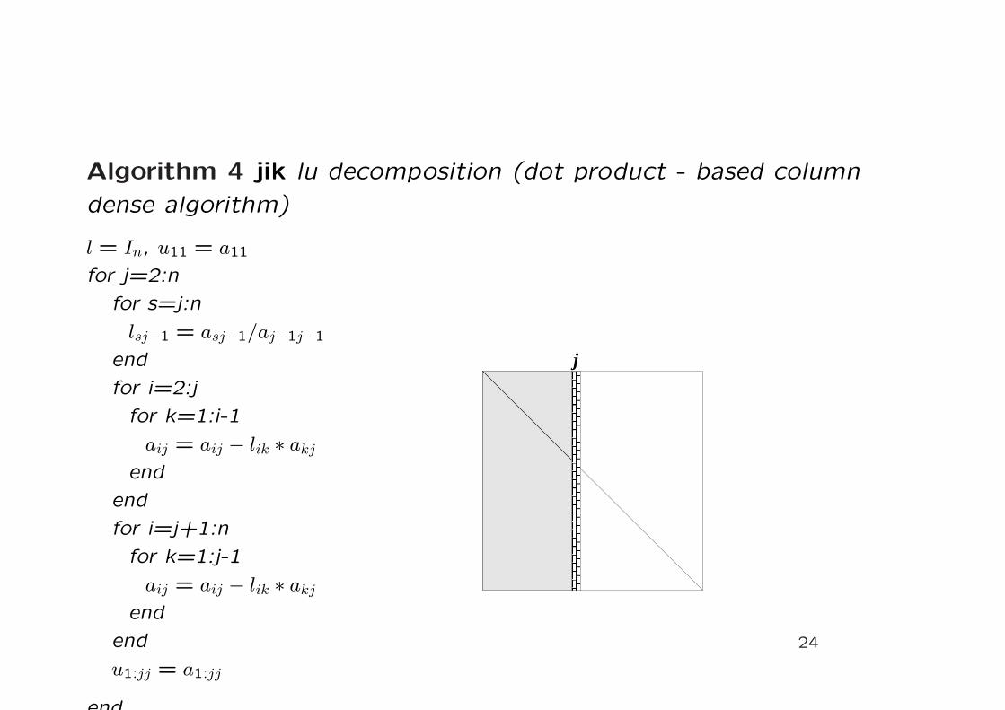
Algorithm 4 jik lu decomposition (dot product - based column
dense algorithm)
l = In, u11 = a11
for j=2:n
for s=j:n
lsj−1 = asj−1/aj−1j−1
end
for i=2:j
for k=1:i-1
aij = aij − lik ∗ akj
end
end
for i=j+1:n
for k=1:j-1
aij = aij − lik ∗ akj
end
end
u1:jj = a1:jj
end
� � �� � �� � �� � �� � �� � �� � �� � �� � �� � �� � �� � �� � �� � �� � �� � �� � �� � �� � �� � �� � �� � �� � �� � �� � �� � �� � �
� �� �� �� �� �� �� �� �� �� �� �� �� �� �� �� �� �� �� �� �� �� �� �� �� �� �� �j
24

Algorithm 5 kij lu decomposition (row oriented submatrix dense
algorithm)
l = In
u = On
for k=1:n-1
for i=k+1:n
lik = aik/akk
for j=k+1:n
aij = aij − lik ∗ akj
end
end
ukk:n = akk:n
end
unn = ann
� � � � � � � � � � � � � � � � � � � � �� � � � � � � � � � � � � � � � � � � � �� � � � � � � � � � � � � � � � � � � � �� � � � � � � � � � � � � � � � � � � � �� � � � � � � � � � � � � � � � � � � � �� � � � � � � � � � � � � � � � � � � � �� � � � � � � � � � � � � � � � � � � � �� � � � � � � � � � � � � � � � � � � � �� � � � � � � � � � � � � � � � � � � � �� � � � � � � � � � � � � � � � � � � � �� � � � � � � � � � � � � � � � � � � � �� � � � � � � � � � � � � � � � � � � � �� � � � � � � � � � � � � � � � � � � � �� � � � � � � � � � � � � � � � � � � � �� � � � � � � � � � � � � � � � � � � � �� � � � � � � � � � � � � � � � � � � � �� � � � � � � � � � � � � � � � � � � � �� � � � � � � � � � � � � � � � � � � � �� � � � � � � � � � � � � � � � � � � � �� � � � � � � � � � � � � � � � � � � � �� � � � � � � � � � � � � � � � � � � � �
� � � � � � � � � � � � � � � � � � � � �� � � � � � � � � � � � � � � � � � � � �� � � � � � � � � � � � � � � � � � � � �� � � � � � � � � � � � � � � � � � � � �� � � � � � � � � � � � � � � � � � � � �� � � � � � � � � � � � � � � � � � � � �� � � � � � � � � � � � � � � � � � � � �� � � � � � � � � � � � � � � � � � � � �� � � � � � � � � � � � � � � � � � � � �� � � � � � � � � � � � � � � � � � � � �� � � � � � � � � � � � � � � � � � � � �� � � � � � � � � � � � � � � � � � � � �� � � � � � � � � � � � � � � � � � � � �� � � � � � � � � � � � � � � � � � � � �� � � � � � � � � � � � � � � � � � � � �� � � � � � � � � � � � � � � � � � � � �� � � � � � � � � � � � � � � � � � � � �� � � � � � � � � � � � � � � � � � � � �� � � � � � � � � � � � � � � � � � � � �� � � � � � � � � � � � � � � � � � � � �� � � � � � � � � � � � � � � � � � � � �k
25

Algorithm 6 kji lu decomposition (column oriented submatrix
dense algorithm)
l = In, u = On
for k=1:n-1
for s=k+1:n
lsk = as,k/ak,k
end
for j=k+1:n
for i=k+1:n
aij = aij − lik ∗ akj
end
end
ukk:n = akk:n
end
unn = ann
� � � � � � � � � � � � � � � � � � � � �� � � � � � � � � � � � � � � � � � � � �� � � � � � � � � � � � � � � � � � � � �� � � � � � � � � � � � � � � � � � � � �� � � � � � � � � � � � � � � � � � � � �� � � � � � � � � � � � � � � � � � � � �� � � � � � � � � � � � � � � � � � � � �� � � � � � � � � � � � � � � � � � � � �� � � � � � � � � � � � � � � � � � � � �� � � � � � � � � � � � � � � � � � � � �� � � � � � � � � � � � � � � � � � � � �� � � � � � � � � � � � � � � � � � � � �� � � � � � � � � � � � � � � � � � � � �� � � � � � � � � � � � � � � � � � � � �� � � � � � � � � � � � � � � � � � � � �� � � � � � � � � � � � � � � � � � � � �� � � � � � � � � � � � � � � � � � � � �� � � � � � � � � � � � � � � � � � � � �� � � � � � � � � � � � � � � � � � � � �� � � � � � � � � � � � � � � � � � � � �� � � � � � � � � � � � � � � � � � � � �
� � � � � � � � � � � � � � � � � � � � �� � � � � � � � � � � � � � � � � � � � �� � � � � � � � � � � � � � � � � � � � �� � � � � � � � � � � � � � � � � � � � �� � � � � � � � � � � � � � � � � � � � �� � � � � � � � � � � � � � � � � � � � �� � � � � � � � � � � � � � � � � � � � �� � � � � � � � � � � � � � � � � � � � �� � � � � � � � � � � � � � � � � � � � �� � � � � � � � � � � � � � � � � � � � �� � � � � � � � � � � � � � � � � � � � �� � � � � � � � � � � � � � � � � � � � �� � � � � � � � � � � � � � � � � � � � �� � � � � � � � � � � � � � � � � � � � �� � � � � � � � � � � � � � � � � � � � �� � � � � � � � � � � � � � � � � � � � �� � � � � � � � � � � � � � � � � � � � �� � � � � � � � � � � � � � � � � � � � �� � � � � � � � � � � � � � � � � � � � �� � � � � � � � � � � � � � � � � � � � �� � � � � � � � � � � � � � � � � � � � �k
26

2.b) Sparse direct methods: existence of fill-in
• Not all the algorithms equally desirable when A is sparse
• The problem: sparsity structure of L+U (L+LT , L+B+LT )
do not need to be the same as the sparsity structure of A:
new nonzeros (fill-in) may arise
0 50 100 150 200 250 300 350 400
0
50
100
150
200
250
300
350
4000 50 100 150 200 250 300 350 400
0
50
100
150
200
250
300
350
400
27

2.b) Sparse direct methods: fill-in
• Arrow matrix
∗ ∗ ∗ ∗ ∗∗ ∗∗ ∗∗ ∗∗ ∗
∗ ∗∗ ∗∗ ∗∗ ∗
∗ ∗ ∗ ∗ ∗
• How to describe the fill-in
• How to avoid it
28

2.b) Sparse direct methods: fill-in description
Definition 9 Sequence of elimination matrices: A(0) ≡ A, A(1),
A(2), . . ., A(n): computed entries from factors replace original
(zero and nonzero) entries of A.
• Local description of fill-in using the matrix structure (entries
of elimination matrices denoted with superscripts in paren-
theses)
• Note that we use the non-cancellation assumption
Lemma 1 (fill-in lemma) Let i > j, k < n. Then
a(k)ij 6= 0 ⇔ a
(k−1)ij 6= 0 or (a(k−1)
ik 6= 0 ∧ a(k−1)kj 6= 0)
29

2.b) Sparse direct methods: fill-in illustration for a
symmetric matrix
30

2.b) Sparse direct methods: fill-in path theorem
• Simple global description via the graph model (follows from
repeated use of fill-in lemma)
Theorem 1 (fill-in path theorem) Let i > j, k < n. Then a(k)ij 6=
0 ⇔ ∃ a path xi, xp1, . . . , xpt, xj in G(A) such that (∀l ∈ t)(pl < k).
31

2.b) Sparse direct methods: path theorem illustration for
a symmetric matrix
*
*
*
*
*
*
** *i
j
k
l
path: i−k, k−l, l−j
32
3. Fill-in in SPD matrices
3.a) Fill-in description: why do we restrict to the SPDcase?
• SPD case enables to separate structural properties of ma-trices from their numerical properties.
• SPD case is simpler and more transparent
• solving sparse SPD systems is very important
• it was historically the first case with a nontrivial insight intothe mechanism of the (Cholesky) decomposition (but not thefirst studied case)
• SPD case enables in many aspects smooth transfer to thegeneral nonsymmetric case
33

3.b) Elimination tree: introduction
• Transparent global description: based on the concept of elim-ination tree (for symmetric matrices) or elimination di-rected acyclic graph (nonsymmetric matrices)
Definition 10 Elimination tree T = (V, E) of a symmetric ma-trix is a rooted tree with V = {x1, . . . , xn}, E = {(xi, xj)|xj =min{k|(k > i) ∧ (lik 6= 0)}}
• Note that it is defined for the structure of L
• Root of the elimination tree: vertex n
• If need we denote vertices only by their indices
• Edges in T connect vertices (i, j) such that i < j
34

3.b) Elimination tree: illustration
∗ ∗ ∗ ∗∗ ∗ ∗ ∗
∗ ∗ ∗∗ ∗ ∗ ∗
∗ ∗ ∗ ∗∗ ∗ ∗ ∗
∗ ∗ ∗∗ ∗ ∗ ∗ ∗ ∗ ∗ ∗
∗ ∗ ∗ ∗∗ ∗ f ∗ ∗
∗ ∗ ∗∗ ∗ ∗ ∗
∗ f ∗ ∗ f ∗∗ ∗ f ∗ f ∗
∗ f ∗ ∗∗ ∗ ∗ ∗ ∗ ∗ ∗ ∗
35
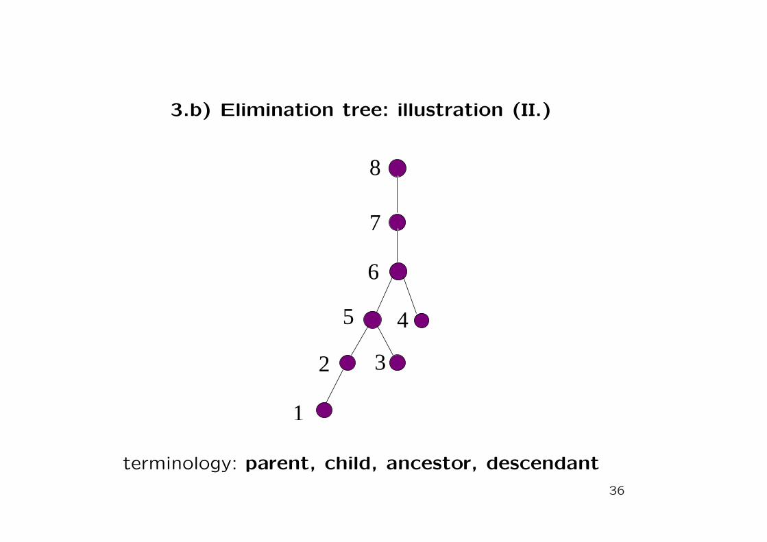
3.b) Elimination tree: illustration (II.)
1
2
5
3
4
6
7
8
terminology: parent, child, ancestor, descendant
36

3.b) Elimination tree: necessary condition for an entry of
L to be (structurally!) nonzero
Lemma 2 If lji 6= 0 then xj is an ancestor of xi in the elimination
tree
37

3.b) Elimination tree: natural source of parallelism
Lemma 3 Let T [xi] and T [xj] be disjoint subtrees of the elimi-
nation tree T . Then lrs = 0 for all xr ∈ T [xi] and xs ∈ T [xj].
x_i x_jT[x_i]
T[x_j]
38

3.b) Elimination tree: full characterization of entries of L
Lemma 4 For j > i we have lji 6= 0 if and only if xi is an ancestor
of some xk in the elimination tree for which ajk 6= 0.
*
*
*
*
*
*
*
*
****
k
i
j
initiating edge edges in G(L)
edge (j,i) in G(L)
j
i
k
39

3.b) Elimination tree: row structure of L is given by a row
subtree of the elimination tree
i
k k’ k’’
k’’’
i
k k’ k’’
k’’’
40
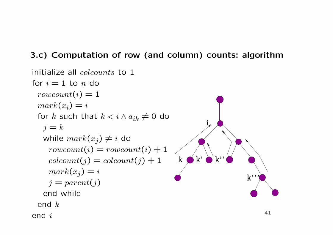
3.c) Computation of row (and column) counts: algorithm
initialize all colcounts to 1
for i = 1 to n do
rowcount(i) = 1
mark(xi) = i
for k such that k < i ∧ aik 6= 0 do
j = k
while mark(xj) 6= i do
rowcount(i) = rowcount(i) + 1
colcount(j) = colcount(j) + 1
mark(xj) = i
j = parent(j)
end while
end k
end i
i
k k’ k’’
k’’’
41
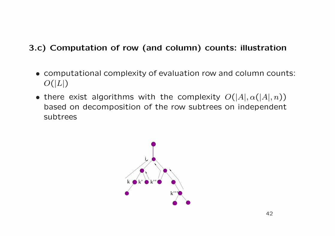
3.c) Computation of row (and column) counts: illustration
• computational complexity of evaluation row and column counts:O(|L|)
• there exist algorithms with the complexity O(|A|, α(|A|, n))based on decomposition of the row subtrees on independentsubtrees
i
k k’ k’’
k’’’
42

3.d) Column structure of L: introduction
Lemma 5 Column j is updated in the decomposition by columns
i such that li,j 6= 0.
Lemma 6
Struct(L∗j) = Struct(A∗j) ∪ ⋃i,lij 6=0 Struct(L∗i) \ {1, . . . , j − 1}.
*
*
*
*
**
*
*
**
*
43

3.d) Column structure of L: an auxiliary result
Lemma 7 Struct(L∗j) {j} ⊆ Struct(L∗parent(j))
44

3.d) Column structure of L: final formula
Consequently:
Struct(L∗j) = Struct(A∗j) ∪⋃
i,j=parent(i)
Struct(L∗i) \ {1, . . . , j − 1}.
This fact directly implies an algorithm to compute
structures of columns
45

3.d) Column structure of L: algorithm
for j = 1 to n dolistxj = ∅
end j
for j = 1 to n docol(j) = adj(xj) \ {x1, . . . , xj−1}for xk ∈ listxj do
col(j) = col(j) ∪ col(k) \ {xj}end xkif col(j) 6= 0 then
p = min{i | xi ∈ col(j)}listxp = listxp ∪ {xj}
end ifend j
end i
46

3.d) Column structure of L: symbolic factorization
• array list stores children of a node
• the fact that parent of a node has a higher label than the
node induce the correctness of the algorithm
• the algorithm for finding structures of columns also called
symbolic factorization
• the derived descriptions used for:
– to allocate space for L
– to store and manage L in static data structures
• needed elimination tree
47

3.e) Elimination tree construction: algorithm
(complexity: O(|A|, α(|A|, n)))
for i = 1 to n do
parent(i) = 0
for k such that xk ∈ adj(xi) ∧ k < i do
j = k
while (parent(j) 6= 0 ∧ parent(j) 6= i) do
r = parent(j)
end while
if parent(j) = 0 then parent(j) = i
end k
end i
i
k k’ k’’
k’’’
48
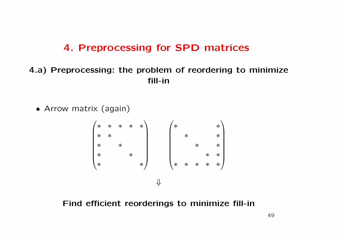
4. Preprocessing for SPD matrices
4.a) Preprocessing: the problem of reordering to minimize
fill-in
• Arrow matrix (again)
∗ ∗ ∗ ∗ ∗∗ ∗∗ ∗∗ ∗∗ ∗
∗ ∗∗ ∗∗ ∗∗ ∗
∗ ∗ ∗ ∗ ∗
⇓
Find efficient reorderings to minimize fill-in
49

4.b) Solving the reordered system: overview
Factorize
PTAP = LLT ,
Compute y from
Ly = PT b,
Compute x from
LTPTx = y.
50

4.c) Static reorderings: local and global reorderings
Static reorderings
• static differs them from dynamic reordering strategies (piv-
oting)
• two basic types
– local reorderings: based on local greedy criterion
– global reorderings: taking into account the whole graph /
matrix
51

4.d) Local reorderings: minimum degree (MD): the basic
algorithm
G = G(A)
for i = 1 to n do
find v such that degG(v) = minv∈V degG(v)
G = Gv
end i
The order of found vertices induces their new renumbering
• deg(v) = |Adj(v)|; graph G as a superscript determines the
current graph
52

4.d) Local reorderings: minimum degree (MD): an
example
v v
G G_v
53

4.d) Local reorderings: minimum degree (MD):
indistinguishability
Definition 11 u a v are called indistinguishable if
AdjG(u) ∪ {u} = AdjG(v) ∪ {v}. (1)
Lemma 8 If u and v are indistinguishable in G and y ∈ V , y 6=u, v. Then u and v are indistinguishable also in Gy.
Corollary 1 Let u and v be indistinguishable in G, y ≡ u has
minimum degree in G. Then v has minimum degree in Gy.
54

4.d) Local reorderings: minimum degree (MD):
indistinguishability (example)
u v u v
G G_v
55

4.d) Local reorderings: minimum degree (MD):dominance
Definition 12 Vertex v is called dominated by u if
AdjG(u){u} ⊆ AdjG(v) ∪ {v}. (2)
Lemma 9 If v is dominated by u in G, and y 6= u, v has minimumdegree in G. Then v is dominated by u also in Gy.
Corollary: Graph degrees do not need to be recomputedfor dominated vertices (using following relations)
v 6∈ AdjG(y) ⇒ AdjGy(v) = AdjG(v) (3)
v ∈ AdjG(y) ⇒ AdjGy(v) = (AdjG(y) ∪AdjG(v))− {y} (4)
56

4.d) Local reorderings: minimum degree (MD):implementation
• graph is represented in a clique representation {K1, . . . , Kq}• – clique: a complete subgraph
57

4.d) Local reorderings: minimum degree (MD):
implementation (II.)
• cliques are being created during the factorization
• they answer the main related question: how to store elimi-
nation graphs with their new edges
Lemma 10
|K| <t∑
i=1
|Ksi|
for merging t cliques Ksi into K.
58
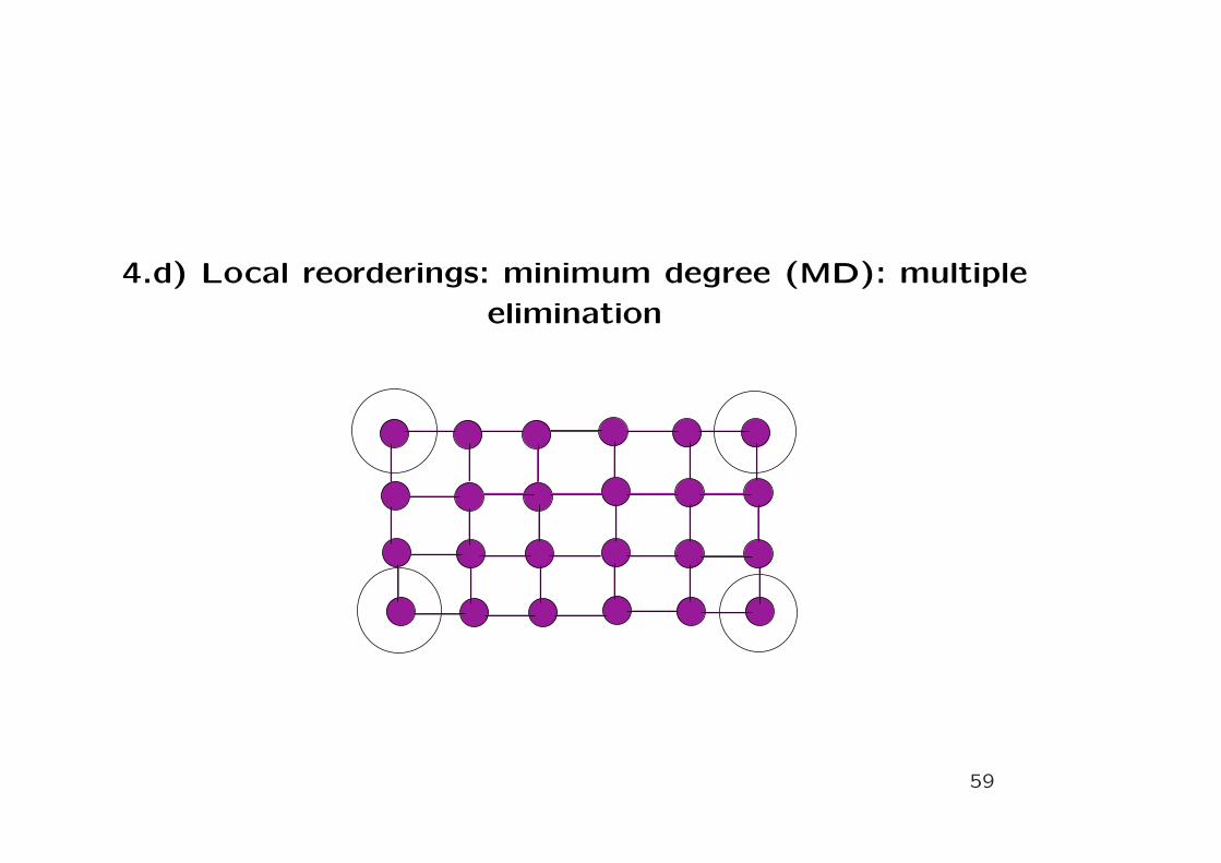
4.d) Local reorderings: minimum degree (MD): multiple
elimination
59

4.d) Local reorderings: minimum degree (MD): MMD
algorithm
G = G(A)
while G 6= ∅find all vj, j = 1, . . . , s such that
degG(vj) = minv∈V (G)degG(v) and adj(vj) ∩ adj(vk) pro j 6= k
for j = 1 to s do
G = Gvj
end for
end while
The order of found vertices induces their new renumbering
60

4.d) Local reorderings: other family members
• MD, MMD with the improvements (cliques, indistinguisha-
bility, dominance, improved clique arithmetic like clique ab-
sorbtions)
• more drastic changes: approximate minimum degree algo-
rithm
• approximate minimum fill algorithms
• in general: local fill-in minimization procedures typically suffer
from lack of tie-breaking strategies – multiple elimination
can be considered as such strategy
61
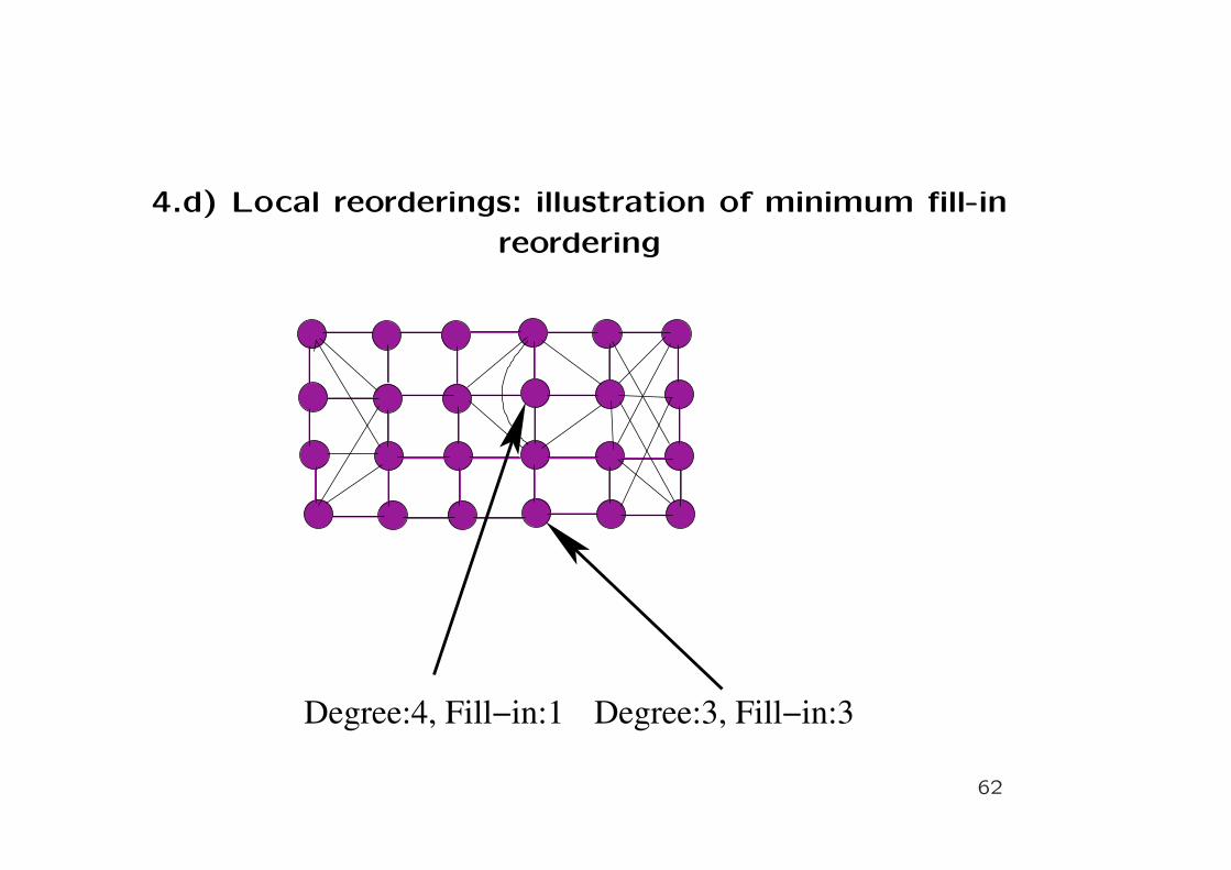
4.d) Local reorderings: illustration of minimum fill-in
reordering
Degree:4, Fill−in:1 Degree:3, Fill−in:3
62

4.e) Global reorderings: nested dissection
Find separator
Reorder the matrix numbering nodes in the separator last
Do it recursively
Vertex separator
C_1 C_2
S
63

4.e) Global reorderings: nested dissection after one level
of recursion
C_1
C_2
S
SC_2C_1
64

4.d) Global reorderings: nested dissection with more levels
1 7 4 43 22 28 25
3 8 6 44 24 29 27
2 9 5 45 23 30 36
19 20 21 46 40 41 42
10 16 13 47 31 37 34
1712 15 48 33 38 36
11 18 14 49 32 39 35
65

4.e) Global reorderings: nested dissection with more
levels: elimination tree
1 2
3
4 5
6
7
8
9
10 11 13 14
12 15
16
17
1819
20
21
22 23
24
25 26
27
28
29
30
31 32
33
34 35
36
37
38
3940
41
42
43
44
45
46
47
48
49
66

4.f) Static reorderings: a preliminary summary
• the most useful strategy: combining local and global re-
orderings
• modern nested dissections are based on graph partitioners:
partition a graph such that
– components have very similar sizes
– separator is small
– can be correctly formulated and solved for a general graph
– theoretical estimates for fill-in and number of operations
• modern local reorderings: used after a few steps of an in-
complete nested dissection
67
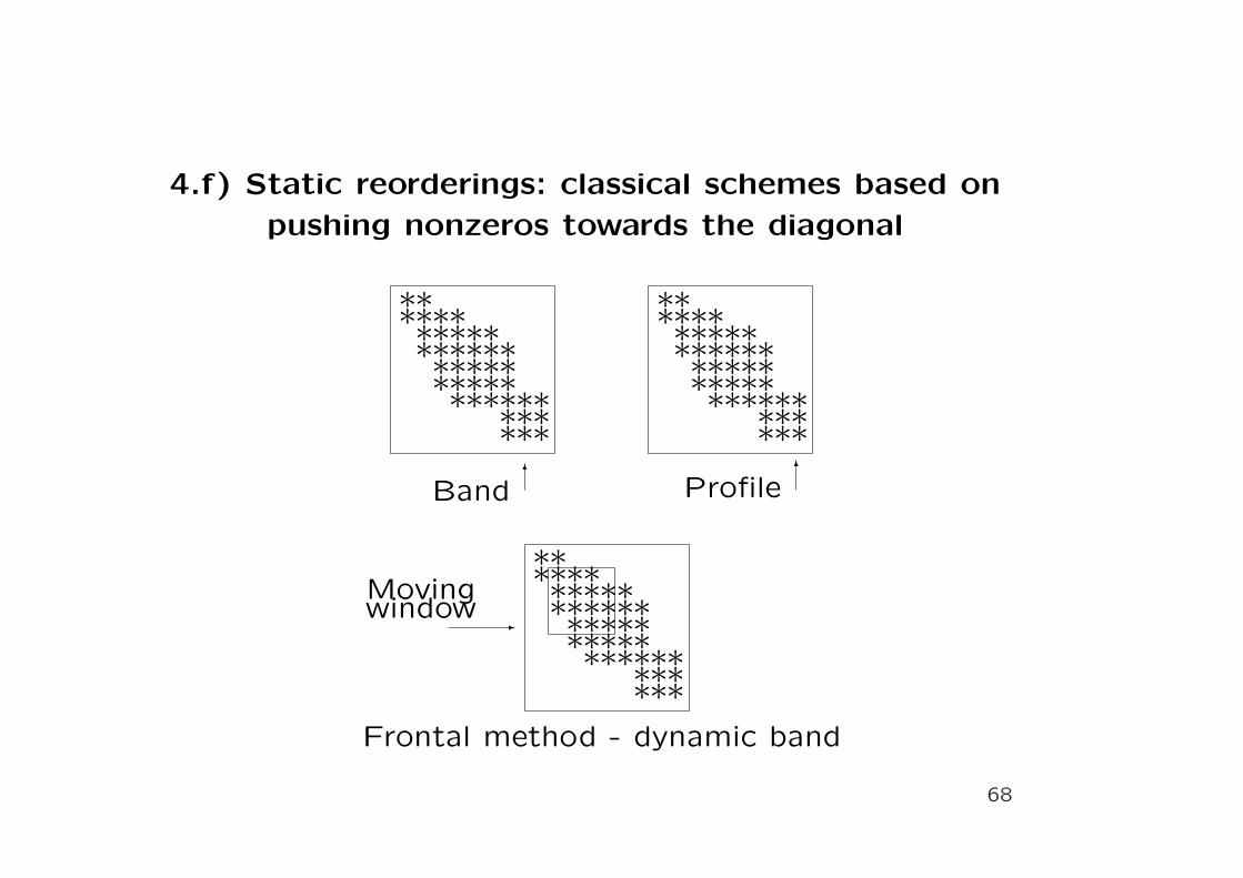
4.f) Static reorderings: classical schemes based on
pushing nonzeros towards the diagonal
****
*******
*******
****
*
**
*******
****
**
*
Band6
****
*******
*******
****
*
**
*******
****
**
*
Profile6
****
*******
*******
****
*
**
*******
****
**
*
Frontal method - dynamic band
Movingwindow
-
68

4.f) Static reorderings: classical schemes based on
pushing nonzeros towards the diagonal: an important
reason for their use
Band(L + LT ) = Band(A)
Profile(L + LT ) = Profile(A)
69
4.f) Static reorderings: classical schemes based onpushing nonzeros towards the diagonal: pros and cons
• +: simple data structure – locality, regularity
• –: structural zeros inside
• +: easy to vectorize
• –: short vectors
• +: easy to use out-of-core
• –: the other schemes are typically more efficient and this ismore important
Evaluation: for general case – more or less historical valueonly; can be important for special matrices, reorderings in
iterative methods70

4.f) Static reorderings: an example of comparison
Example (Liu): 3D finite element discretization of the part of
the automobile chassis =⇒ linear system with a matrix of
dimension 44609. Memory size for the frontal ( = dynamic
band) solver: 52.2 MB; memory size for the general sparse
solver: 5.2MB!
71
5. Algorithmic improvements for SPDdecompositions
5.a) Algorithmic improvements: introduction
• blocks and supernodes: less tolerance to memory latencies
and increase of efective memory bandwidth
• Reorderings based on the elimination tree
72

5.b) Supernodes and blocks: supernodes
Definition 13 Let s, t ∈ Mn such that s + t − 1 ≤ n. Then thecolumns with indices {s, s+1, . . . , s+t−1} form a supernode if thisthe columns satisfy Struct(L∗s) = Struct(L∗s+t−1)∪{s, . . . , s+ t−2}, and the sequence is maximal.
* * * *
* * * ** * * ** * * *
s−t+1
**
**
***
** *
s
73

5.b) Supernodes and blocks: blocks
74

5.b) Supernodes and blocks: some notes
• enormous influence on the efficiency
• different definitions of supernodes and blocks
• blocks found in G(A), supernodes are found in G(L)
• blocks are induced by the application (degrees of freedom in
grid nodes) or efficient algorithms for finding blocks
• efficient algorithms to find supernodes
• complexity: O(|A|)
75

5.c) Reorderings based on the elimination tree:
topological reorderings
Definition 14 Topological reorderings of the elimination tree
are such that each node has smaller index than its parent.
1
2
5
3
4
6
7
8
5
6
7
8
1
2
3
4
Tree with two different topological reorderings
76

5.c) Reorderings based on the elimination tree:
postorderings
Definition 15 Postorderings are topological reorderings where
labels in each rooted subtree form an interval.
1
2
5
3
4
6
7
8
6
7
8
1
Postordered tree
2
3
4 5
77

5.c) Reorderings based on the elimination tree:
postorderings
• Postorderings efficiently use memory hierarchies
• Postorderings are very useful in paging environments
• They are crucial for multifrontal methods
• Even some postorderings are better than the other: trans-
parent description for multifrontal method, see the example
78
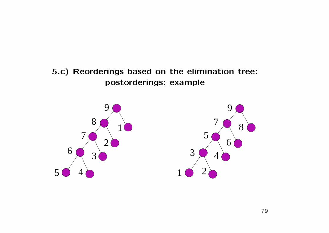
5.c) Reorderings based on the elimination tree:
postorderings: example
5
1
23
4
6
7
8
9 9
1 2
3 4
56
7 8
79

6. Sparse direct methods for SPD matrices
6.a) Algorithmic strategies: introduction
• Some algorithms strongly modified with respect to their
simple dense counterparts because of special data structures
• different symbolic steps for different algorithms
• different amount of overhead
• of course, algorithms provide the same results in exact arith-
metic
80

6.b) Work and memory
• the same number of operations if no additional operationsperformed
• µ(L): number of the arithmetic operations
• η(L) ≡ |L|, η(L∗i): size of the i-th column of L, etc.
|L| =n∑
i=1
η(L∗i) =n∑
i=1
η(Li∗)
µ(L) =n∑
j=1
[η(L∗j)− 1][η(L∗j) + 2]/2
81

6.c) Methods: rough classification
• Columnwise (left-looking) algorithm
• – columns are updated by a linear combination of previouscolumns
• Standard submatrix (right-looking) algorithm
• – non-delayed outer-product updates of the remaining sub-matrix
• Multifrontal algorithm
• – specific efficient delayed outer-product updates
• Each of the algorithms represent a whole class of approaches
• Supernodes, blocks and other enhancements extremely im-portant
82

6.d) Methods: sparse SPD columnwise decomposition
Preprocessing
– prepares the matrix so that the fill-in would be as small aspossible
Symbolic factorization
– determines structures of columns of L. Consequently, L canbe allocated and used for the actual decomposition
– due to a lot of enhancements the boundary between the firsttwo steps is somewhat blurred
Numeric factorization
– the actual decomposition to obtain numerical values of thefactor L
83

6.d) Methods: sparse SPD columnwise decomposition:
numeric decomposition
* * * ******
*
84

6.e) Methods: sparse SPD multifrontal decomposition
• Right-looking method with delayed updates
• The updates are pushed into a stack and popped up only
when needed
• Postorder guarantees having needed updates on the top of
the stack
• some steps of the left-looking SPD modified
85

6.e) Methods: sparse SPD multifrontal decomposition:
illustration
stack
stack
−1
−1
==
= stack
−1=
+ + +
1)
2)
3)
4)
86

7. Sparse direct methods for nonsymmetricsystems
7.a) SPD decompositions versus nonsymmetric
decompositions
• LU factorization instead of Cholesky
• nonsymmetric (row/column) permutations needed for both
sparsity preservation and maintaining numerical stability
• consequently: dynamic reorderings (pivoting) needed
• a different model for fill-in analysis: generalizing the elimina-
tion tree
87