Sketching Sparse Matrices

Gautam Dasarathy, Parikshit Shah, Badri Narayan Bhaskar, and Rob NowakUniversity of Wisconsin - Madison

March 26, 2013

Abstract

This paper considers the problem of recovering an unknown sparse p⇥ p matrix Xfrom an m ⇥ m matrix Y = AXBT , where A and B are known m ⇥ p matrices withm ⌧ p.

The main result shows that there exist constructions of the “sketching” matrices Aand B so that even if X has O(p) non-zeros, it can be recovered exactly and e�cientlyusing a convex program as long as these non-zeros are not concentrated in any singlerow/column of X. Furthermore, it su�ces for the size of Y (the sketch dimension) toscale as m = O �p # nonzeros in X ⇥ log p

�. The results also show that the recovery is

robust and stable in the sense that if X is equal to a sparse matrix plus a perturbation,then the convex program we propose produces an approximation with accuracy pro-portional to the size of the perturbation. Unlike traditional results on sparse recovery,where the sensing matrix produces independent measurements, our sensing operator ishighly constrained (it assumes a tensor product structure). Therefore, proving recov-ery guarantees require non-standard techniques. Indeed our approach relies on a novelresult concerning tensor products of bipartite graphs, which may be of independentinterest.

This problem is motivated by the following application, among others. Considera p ⇥ n data matrix D, consisting of n observations of p variables. Assume that thecorrelation matrix X := DDT is (approximately) sparse in the sense that each of the pvariables is significantly correlated with only a few others. Our results show that thesesignificant correlations can be detected even if we have access to only a sketch of thedata S = AD with A 2 Rm⇥p.

Keywords. sketching, tensor products, distributed sparsity, `1 minimization, compressedsensing, covariance sketching, graph sketching, multi-dimensional signal processing.

1 Introduction

An important feature of many modern data analysis problems is the presence of a largenumber of variables relative to the amount of available resources. Such high dimensionality

1

arX

iv:1

303.

6544

v1 [

cs.IT

] 26

Mar

201

3

occurs in a range of applications in bioinformatics, climate studies, and economics. Accord-ingly, a fruitful and active research agenda over the last few years has been the developmentof methods for sampling, estimation, and learning that take into account structure in theunderlying model and thereby making these problems tractable. A notion of structure thathas seen many applications is that of sparsity, and methods for sampling and estimatingsparse signals have been the subject of intense research in the past few years [11, 10, 20]

In this paper we will study a more nuanced notion of structure which we call distributedsparsity. For what follows, it will be convenient to think of the unknown high-dimensionalsignal of interest as being represented as a matrix X. Roughly, the signal is said to bedistributed sparse if every row and every column of X has only a few non-zeros. We will seethat it is possible to design e�cient and e↵ective acquisition and estimation mechanisms forsuch signals. Let us begin by considering a few example scenarios where one might encounterdistributed sparsity.

• Covariance Matrices: Covariance matrices associated to some natural phenomenahave the property that each covariate is correlated with only a few other covariates.For instance, it is observed that protein signaling networks are such that there areonly a few significant correlations [45] and hence the discovery of the such networksfrom experimental data naturally leads to the estimation of a covariance matrix (wherethe covariates are proteins) which is (approximately) distributed sparse. Similarly, thecovariance structure corresponding to longitudinal data is distributed sparse [17]. SeeSection 1.3.1.

• Multi-dimensional signals: Multi-dimensional signals such as the natural imagesthat arise in medical imaging [11] are known to be sparse in the gradient domain. Whenthe features in the images are not axis-aligned, not only is the matrix representationof the image gradient sparse, it is also distributed sparse. For a little more on this, seeSection 1.3.3

• Random Sparse Signals and Random Graphs: Signals where the sparsity patternis random (i.e., each entry is nonzero independently and with a probability q) are alsodistributed sparse with high probability. The “distributedness” of the sparsity patterncan be measured using the “degree of sparsity” d which is defined to be the maximumnumber of non-zeros in any row or column. For random sparsity patterns, we have thefollowing:

Proposition 1. Consider a random matrix X 2 Rp⇥p whose entries are independentcopies of the Bernoulli(�) 1distribution where p� = � = ⇥(1). Then for any ✏ > 0, Xhas at most d 1’s in each row/column with probability at least 1� ✏, where

d = �

✓1 +

2 log(2p/✏)

�

◆.

1Recall that if � ⇠ Bernoulli(�), then P (� = 1) = � and P (� = 0) = 1 � �.

2

(The proof is straightforward, and available in Appendix B.)

In a similar vein, combinatorial graphs have small degree in a variety of applications,and their corresponding matrix representation will then be distributed sparse. Forinstance, Erdos-Renyi random graphs G(p, q) with pq = O(log p) have small degree [9].

1.1 Problem Setup and Main Results

Our goal is to invert an underdetermined linear system of the form

Y = AXB

T, (1)

where A = [aij] 2 Rm⇥p, B = [bij] 2 Rm⇥p, with m ⌧ p and X 2 Rp⇥p. Since the matrix

X 2 Rp⇥p is linearly transformed to obtain the smaller dimensional matrix Y 2 Rm⇥m, wewill refer to Y as the sketch (borrowing terminology from the computer science literature[40]) of X and we will refer to the quantity m as the sketching dimension. Since the valueof m signifies the amount of compression achieved, it is desirable to have as small a value ofm as possible.

Rewriting the above using tensor product notation, with y = vec(Y ) and x = vec(X),we equivalently have

y = (B ⌦ A)x, (2)

where vec(X) simply vectorizes the matrix X, i.e., produces a long column vector by stackingthe columns of the matrix and B⌦A is the tensor (or Kronecker) product of B and A, givenby 2

6664

b11A b12A · · · b1pA

b21A b22A · · · b2pA

......

. . ....

bm1A bm2A · · · bmpA

3

7775. (3)

While it is not possible to invert such underdetermined systems of equations in gen-eral, the rapidly growing literature on what has come to be known as compressed sensingsuggests that this can be done under certain assumptions. In particular, taking cues fromthis literature, one might think that this is possible if x (or equivalently X) has only a fewnon-zeros.

Let us first consider the case when there are only k = ⇥(1) non-zeros in X, i.e., it is verysparse. Then, it is possible to prove that the optimization program (P1) recovers X fromAXB

T using standard “RIP-based” techniques [11]. We refer the interested reader to thepapers by Jokar et al [33] and Duarte et al [21] for more details, but in essence the authorsshow that if �r(A) and �r(B) are the restricted isometry constants (of order r) [11] for A andB respectively, then the following is true about B ⌦ A

max {�r(A), �r(B)} �r(A⌦ B) = �r(B ⌦ A) (1 + �r(A)) (1 + �r(B))� 1.

In many interesting problems that arise naturally, as we will see in subsequent sections,a more realistic assumption to make is that X has O(p) non-zeros and it is this setting we

3

consider for this paper. Unfortunately, the proof techniques outlined above cannot succeedin such a demanding scenario. As hinted earlier, it will turn out however that one cannothandle arbitrary sparsity patterns and that the non-zero pattern ofX needs to be distributed,i.e., each row/column of X cannot have more than a few, say d, non-zeros. We will call suchmatrices d�distributed sparse (see Definition 3). We explore this notion of structure in moredetail in Section 3.1.

An obvious, albeit highly impractical, approach to recover a (distributed) sparse X frommeasurements of the form Y = AXB

T is the following: search over all matrices X 2 Rp⇥p

such that AXB

T agrees with Y = AXB

T and find the sparsest one. One might hope thatunder reasonable assumptions, such a procedure would return X as the solution. However,there is no guarantee that this approach might work and worse still, such a search procedureis known to be computationally infeasible.

We instead consider solving the optimization program (P1) which is a natural (convex)relaxation of the above approach.

minimizeX

���X���1

subject to AXB

T = Y.

(P1)

Here, by kXk1 we meanP

i,j

���Xi,j

���, i.e., the `1 norm of vec(X).

The main part of the paper is devoted to showing with high probability (P1) has a uniquesolution that equals X. In particular, we prove the following result.

Theorem 1. Suppose that X is d�distributed sparse. Also, suppose that A,B 2 {0, 1}m⇥p

are drawn independently and uniformly from the ��random bipartite ensemble2. Then aslong as

m = O(p

dp log p) and � = O(log p),

there exists a c > 0 such that the optimal solution X

⇤ of (P1) equals X with probabilityexceeding 1� p

�c. Furthermore, this holds even if B equals A.

In Section 4, we will prove Theorem 1 for the case when B = A. It is quite straightforwardto modify this proof to the case where A and B are independently drawn, since there is muchmore independence that can be leveraged.

Let us pause here and consider some implications of this theorem.

1. (P1) does not impose any structural restrictions on X

⇤. In other words, even thoughX is assumed to be distributed sparse, this (highly non-convex) constraint need not befactored in to the optimization problem. This ensures that (P1) is a Linear Program(see e.g., [6]) and can thus be solved e�ciently.

2Roughly speaking, the ��random bipartite ensemble consists of the set of all 0-1 matrices that havealmost exactly � ones per column. We refer the reader to Definition 4 for the precise definition and Section 3.2for more details.

4

2. Recall that what we observe can be thought of as the Rm2vector

(B ⌦ A)x. Since X is d�distributed sparse, x has O(dp) non-zeros. Now, even ifan oracle were to reveal the exact locations of these non-zeros, we would require atleast O(dp) measurements to be able to perform the necessary inversion to recoverx. In other words, it is absolutely necessary for m2 to be at least O(dp). Comparingthis to Theorem 1 shows that the simple algorithm we propose is near optimal in thesense that it is only a logarithm away from this trivial lower bound. This logarithmicfactor also makes an appearance in the measurement bounds in the compressed sensingliterature [10].

3. Finally, as mentioned earlier, inversion of under-determined linear systems where thelinear operator assumes a tensor product structure has been studied earlier [32, 22].However, these methods are relevant only in the regime where the sparsity of thesignal to be recovered is much smaller than the dimension p. The proof techniquesthey employ will unfortunately not allow one to handle the more demanding situationthe sparsity scales linearly in p and if one attempted an extension of their techniquesnaively to this situation, one would see that the sketch size m needs to scale likeO(dp log2 p) in order to recover a d� distributed sparse matrix X. This is of courseuninteresting since it would imply that the size of the sketch is bigger than the size ofX.

It is possible that Y was not exactly observed, but rather is only available to us as a cor-rupted version Y . For instance, Y could be Y corrupted by independent zero mean, additiveGaussian noise or in case of the covariance sketching problem discussed in Section 1.3.1, Ycould be an empirical estimate of the covariance matrix Y = AXA

T . In both these cases, anatural relaxation to (P1) would be the following optimization program (P2) (with B set toA in the latter case).

minimizeX

kAXB

T � Y k22 + �

���X���1

(P2)

Notice that if X was a sparse covariance matrix and if A = B = Ip⇥p, then (P2) reduces tothe soft thresholding estimator of sparse covariance matrices studied in [43].

While our experimental results show that this optimization program (P2) performs well,we leave its exploration and analysis to future work. We will instead state the following“approximation” result that shows that the solution of (P1) is close to the optimal d�distributed sparse approximation for any matrix X. The proof is similar to the proof ofTheorem 3 in [5] and is provided in Appendix C. Given p 2 N, let [p] denote the set{1, 2, . . . , p} and let Wd,p denote the following collection of subsets of [p]⇥ [p]:

Wd,p := {⌦ ⇢ [p]⇥ [p] : |⌦ \ {{i}⇥ [p]}| d, |⌦ \ {[p]⇥ {i}}| d, for all i 2 [p]} .

Notice that if a matrix X 2 Rp⇥p is such that there exists an ⌦ 2 Wd,p with the propertythat Xij 6= 0 only if (i, j) 2 ⌦, then the matrix is d�distributed sparse.

5

Given ⌦ 2 Wd,p and a matrix X 2 Rp⇥p, we write X⌦ to denote the projection of X ontothe set of all matrices supported on ⌦. That is,

[X⌦]i,j =

(Xi,j if (i, j) 2 ⌦0 otherwise

for all (i, j) 2 [p]⇥ [p].

Theorem 2. Suppose that X is an arbitrary p ⇥ p matrix and that the hypotheses of The-orem 1 hold. Let X

⇤ denote the solution to the optimization program (P1). Then, thereexist constants c > 0 and ✏ 2 (0, 1/4) such that the following holds with probability exceeding1� p

�c.

kX⇤ �Xk1 2� 4✏

1� 4✏

✓min

⌦2Wd,p

kX �X⌦k1◆. (4)

The above theorem tells us that even if X is not structured in any way, the solution ofthe optimization program (P1) approximates X as well as the best possible d�distributedsparse approximation of X (up to a constant factor). This has interesting implications, forinstance, to situations where a d�distributed sparse X is corrupted by a “noise” matrix N

as shown in the following corollary.

Corollary 1. Suppose X 2 Rp⇥p is d�distributed sparse and suppose that X = X + N .Then, the solution X

⇤ to the optimization program

min.X

���X���1subject to AXB

T = AXB

T

satisfies

kX⇤ �Xk1 5� 12✏

1� 4✏kNk1 (5)

Proof. Let ⌦ be the support of X. To prove the result, we will consider the following chainof inequalities.

kX⇤ �Xk1 ���X⇤ � X

���1+���X �X

���1

(a)

2� 4✏

1� 4✏

���X � X⌦

���1+���X �X

���1

2� 4✏

1� 4✏

���X �X

���1+

2� 4✏

1� 4✏

���X⌦ �X

���1+���X �X

���1

(b)

5� 12✏

1� 4✏

���X �X

���1

(c)=

5� 12✏

1� 4✏kNk1 .

Here (a) follows from Theorem 2 since ⌦ 2 Wd,p and (b) follows from the fact that���X⌦ �X

��� ���X �X

��� since X⌦c is 0p⇥p. Finally, in (c) we merely plug in the definition of

X.

6

1.2 The Rectangular Case and Higher Dimensional Signals

While Theorem 1, as stated, applies only to the case of square matrices X, we can extend ourresult in a straightforward manner to the rectangular case. Consider a matrix X 2 Rp1⇥p2

where (without loss of generality) p1 < p2. We assume that the row degree is dr (i.e. norow of X has more than dr non-zeros) and that the column degree is dc. Consider sketchingmatrices A 2 Rm⇥p1 and B 2 Rm⇥p2 and the sketching operation:

Y = AXB

T.

Then we have the following corollary:

Corollary 2. Suppose that X is distributed sparse with row degree dr and colum degree dc.Also, suppose that A 2 {0, 1}m⇥p1, B 2 {0, 1}m⇥p2 are drawn independently and uniformlyfrom the ��random bipartite ensemble. Let us define p = max(p1, p2) and d = max(dr, dc).

Then ifm = O(

pdp log p) and � = O(log p),

there exists a c > 0 such that the optimal solution X

⇤ of (P1) equals X with probabilityexceeding 1� p

�c.

Proof. Let us define the matrix X 2 Rp⇥p as

X =

X

0

�,

i.e. it is made square by padding additional zero rows. Note that X has degree d =max(dr, dc). Moreover note that the matrix A 2 Rm⇥p1 can be augmented to A 2 Rm⇥p via:

A =⇥A A

⇤

where A 2 Rm⇥(p�p1) is also drawn from the �-random bipartite ensemble. Then one has therelation:

Y = AXB

T.

Thus, the rectangular problem can be reduced to the standard square case considered inTheorem 1, and the result follows.

The above result shows that a finer analysis is required for the rectangular case. Forinstance, if one were to consider a scenario where p1 = 1, then from the compressed sensingliterature, we know that the result of Corollary 2 is weak. We believe that determining theright scaling of the sketch dimension(s) in the case when X is rectangular is an interestingavenue for future work.

Finally, we must also state that while the results in this paper only deal with two-dimensional signals, similar techniques can be used to deal with higher dimensional tensorsthat are distributed sparse. We leave a detailed exploration of this question to future work.

7

1.3 Applications

It is instructive at this stage to consider a few examples of the framework we set up in thispaper. These applications demonstrate that the modeling assumptions we make viz., tensorproduct sensing and distributed sparsity are important and arise naturally in a wide varietyof contexts.

1.3.1 Covariance Estimation from Compressed realizationsor Covariance Sketching

One particular application that will be of interest to us is the estimation of covariancematrices from sketches of the sample vectors. We call this covariance sketching.

Consider a scenario in which the covariance matrix ⌃ 2 Rp⇥p of a high-dimensionalzero-mean random vector ⇠ = (⇠1, . . . , ⇠p)T is to be estimated. In many applications ofinterest, one determines ⌃ by conducting correlation tests for each pair of covariates ⇠i, ⇠j andcomputing an estimate of E[⇠i⇠j] for i, j = 1, . . . , p. This requires one to perform correlationtests for O(p2) pairs of covariates, a daunting task in the high-dimensional setting. Perhapsmost importantly, in many cases of interest, the underlying covariance matrix may havestructure, which such an approach may fail to exploit. For instance if ⌃ is very sparse, itwould be vastly more e�cient to perform correlation tests corresponding to only the non-zeroentries. The chief di�culty of course is that the sparsity pattern is rarely known in advance,and finding this is often the objective of the experiment.

In other settings of interest, one may obtain statistical samples by observing n indepen-dent sample paths of the statistical process. When ⇠ is high-dimensional, it may be infeasibleor undesirable to sample and store the entire sample paths ⇠(1), . . . , ⇠(n) 2 Rp, and it may bedesirable to reduce the dimensionality of the acquired samples.

Thus in the high-dimensional setting we propose an alternative acquisition mechanism:pool covariates together to form a collection of new variables Z1, . . . , Zm, where m < p. Forexample one may construct:

Z1 = ⇠1 + ⇠2 + ⇠6, Z2 = ⇠1 + ⇠4 + ⇠8 + ⇠12, . . .

and so on; more generally we have measurements of the form Z = A⇠ where A 2 Rm⇥p andtypically m ⌧ p. We call the thus newly constructed covariates Z = (Z1, . . . , Zm) a sketchof the random vector ⇠.

More formally, the covariance sketching problem can be stated as follows. Let ⇠(1), ⇠(2), . . . , ⇠(n) 2Rp be n independent and identically distributed p�variate random vectors and let ⌃ 2 Rp⇥p

be their unknown covariance matrix. Now, suppose that one has access to them�dimensionalsketch vectors Z

(i) such that

Z

(i) = A⇠

(i), i = 1, 2, . . . , n,

where A 2 Rm⇥p,m < p is what we call a sketching matrix. The goal then is to recover

⌃ using only {Z(i)}ni=1. The sketching matrices we will focus on later will have randomly-generated binary values, so each element of Z(i) will turn out to be a sum (or “pool”) of arandom subset of the covariates.

8

Notice that the sample covariance matrix computed using the vectors�Z

(i) ni=1

satisfiesthe following.

⌃(n)Z :=

1

n

nX

i=1

Z

(i)(Z(i))T

= A

1

n

nX

i=1

⇠

(i)(⇠(i))T!A

T

= A⌃(n)A

T,

where ⌃(n) := 1n

Pni=1 ⇠

(i)(⇠(i))T is the (maximum likelihood) estimate of ⌃ from the samples⇠

(1). . . , ⇠

(n).To gain a better understanding of the covariance sketching problem, it is natural to first

consider the stylized version of the problem suggested by the above calculation. That is,whether it is possible to e�ciently recover a matrix ⌃ 2 Rp⇥p given the ideal covariancematrix of the sketches ⌃Z = A⌃AT 2 Rm⇥m. The analysis in the current paper focuses onexactly this problem and thus helps in exposing the most unique and challenging aspects ofcovariance sketching.

The theory developed in this paper tells us that at the very least, one needs to restrictthe underlying random vector ⇠ to have the property that each ⇠i depends on only a few (say,d) of the other ⇠j’s. Notice that this would of course imply that the true covariance matrix⌃ will be d�distributed sparse. Applying Theorem 1, especially the version in which thematrices A and B are identical, to this stylized situation reveals the following result. If A ischosen from a particular random ensemble and if one gets to observe the covariance matrixA⌃AT of the sketch random vector Z = A⇠, then using a very e�cient convex optimizationprogram, one can recover ⌃ exactly.

Now, suppose that ⇠ and A are as above and that we get to observe n samples Z

(i) =A⇠

(i), i = 1, 2, . . . , n of the sketch Z = A⇠. Notice that we can can consider ⌃(n) :=

1n

Pni=1 ⇠

(i)(⇠(i))T to be a “noise corrupted version” of ⌃ since we can write

⌃(n) = ⌃+ (⌃(n) � ⌃),

where, under reasonable assumptions on the underlying distribution,���⌃(n) � ⌃���1! 0 almost surely as n ! 1 by the strong law of large of numbers. Therefore,

an application of Theorem 2 tells us that solving (P1) with the observation matrix ⌃(n)Z gives

us an asymptotically consistent procedure to estimate the covariance matrix ⌃ from sketchedrealizations.

We anticipate that our results will be interesting in many areas such as quantitativebiology where it may be possible to naturally pool together covariates and measure interac-tions at this pool level. Our work shows that covariance structures that occur naturally areamenable to covariance sketching, so that drastic savings are possible when correlation testsare performed at the pool level, rather than using individual covariates.

9

The framework we develop in this paper can also be used to accomplish cross covariancesketching. That is, suppose that ⇠ and ⇣ are two zero mean p�variate random vectors andsuppose that ⌃⇠⇣ 2 Rp⇥p is an unknown matrix such that [⌃⇠⇣ ]ij = E[⇠i⇣j]. Let {⇠(i)}ni=1

and {⇣(i)}ni=1 be 2n independent and identically distributed random realizations of ⇠ and ⇣respectively. The goal then, is to estimate ⌃⇠⇣ from the m dimensional sketch vectors Z

(i)

and W

(i) such thatZ

(i) = A⇠

(i),W

(i) = B⇣

(i)i = 1, 2, . . . , n,

where A,B 2 Rm⇥p,m < p.

As above, in the idealized case, Theorem 1 shows that the cross-covariance matrix ⌃⇠⇣

of ⇠ and ⇣ can be exactly recovered from the cross-covariance matrix ⌃ZW = A⌃⇠⇣BT of

the sketched random vectors W and Z as long as ⌃⇠⇣ is distributed sparse. In the case wehave n samples each of the sketched random vectors, an application of Theorem 2 to thisproblem tells us that (P1) is an e�cient and asymptotically consistent procedure to estimatea distributed sparse ⌃⇠⇣ from compressed realization of ⇠ and ⇣.

We note that the idea of pooling information in statistics, especially in the context ofmeta analysis is a classical one [29]. For instance the classical Cohen’s d estimate uses theidea of pooling samples obtained from di↵erent distributions to obtain accurate estimatesof a common variance. While at a high level the idea of pooling is related, we note thatour notion is qualitatively di↵erent in that we propose pooling covariates themselves intosketches and obtain samples in this reduced dimensional space.

1.3.2 Graph Sketching

Large graphs play an important role in many prominent problems of current interest; twosuch examples are graphs associated to communication networks (such as the internet) andsocial networks. Due to their large sizes it is di�cult to store, communicate, and analyzethese graphs, and it is desirable to compress these graphs so that these tasks are easier. Theproblem of compressing or sketching graphs has recently gained attention in the literature[1, 24].

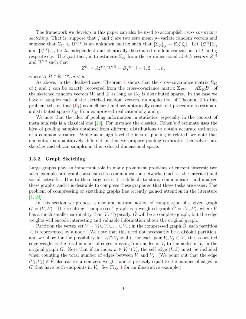
In this section we propose a new and natural notion of compression of a given graphG = (V,E). The resulting “compressed” graph is a weighted graph G = (V , E), where V

has a much smaller cardinality than V . Typically, G will be a complete graph, but the edgeweights will encode interesting and valuable information about the original graph.

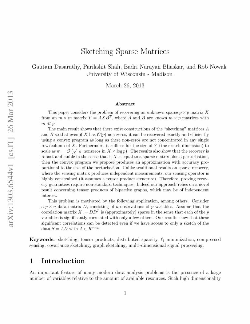
Partition the vertex set V = V1[V2[ . . .[Vm; in the compressed graph G, each partitionVi is represented by a node. (We note that this need not necessarily be a disjoint partition,and we allow for the possibility for Vi \ Vj 6= ;.) For each pair Vi, Vj 2 V , the associatededge weight is the total number of edges crossing from nodes in Vi to the nodes in Vj in theoriginal graph G. Note that if an index k 2 Vi \ Vj, the self edge (k, k) must be includedwhen counting the total number of edges between Vi and Vj. (We point out that the edge(Vk, Vk) 2 E also carries a non-zero weight; and is precisely equal to the number of edges inG that have both endpoints in Vk. See Fig. 1 for an illustrative example.)

10

Define Ai to be the (row) indicator vector for the set Vi, i.e.

Aij =

⇢1 if j 2 Vi

0 otherwise

If X denotes the adjacency matrix of G, then Y := AXA

T denotes the matrix representationof G. The sketch Y has two interesting properties:

• The encoding faithfully preserves high-level “cut” information about the original graph.For instance information such as the weight of edges crossing between the partitionsVi and Vj is faithfully encoded. This could be useful for networks where the vertexpartitions have a natural interpretation such as geographical regions; questions aboutthe total network capacity between two regions is directly available via this method ofencoding a graph. Approximate solutions to related questions such as maximum flowbetween two regions (partitions) can also be provided by solving the problem on thecompressed graph.

• When the graph is bounded degree, the results in this paper show that there exists asuitable random partitioning scheme such that the proposed method of encoding thegraph is lossless. Moreover, the original graph G can be unravelled from the smallersketched graph G e�ciently using the convex program (P1).

V1 V2

V3 V4

24

3

02

3

1

(a) (b) (c)

3

3

2

V1 V2

V3 V4

Figure 1: An example illustrating graph sketching. (a) A graph G with 17 nodes (b) Parti-tioning the nodes into four partitions V1, V2, V3, V4 (c) The sketch of the graph G. The nodesrepresent the partitions and the edges in the sketch represent the total number of edges ofG that cross partitions.

1.3.3 Multidimensional Signal Processing

Multi-dimensional signals arise in a variety of applications, for instance images are naturallyrepresented as two-dimensional signals f(·, ·) over some given domain.

Often it is more convenient to view the signal not in the original domain, but ratherin a transformed domain. Given some one dimensional family of “mother” functions u(t)

11

(usually an orthonormal family of functions indexed with respect to the transform variableu), such a family induces the transform for a one dimensional signal f(t) (with domain T )via

f(u) =

Z

t2Tf(t) u(t).

For instance if u(t) := exp(�i2⇡ut), this is the Fourier transform, and if u(t) is chosen tobe a wavelet function (where u = (a, b), the translation and scale parameters respectively)this generates the well-known wavelet transform that is now ubiquitous in signal processing.

Using u(t) to form an orthonormal basis for one-dimensional signals, it is straightforwardto extend to a basis for two-dimensional signal by using the functions u(t) v(r). Indeed,this defines a two-dimensional transform via

f(u, v) =

Z

(t,r)2X⇥Xf(t, r) u(t) v(r).

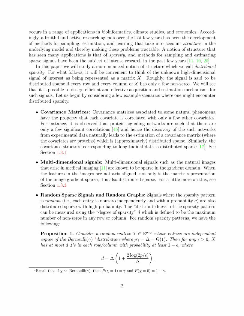
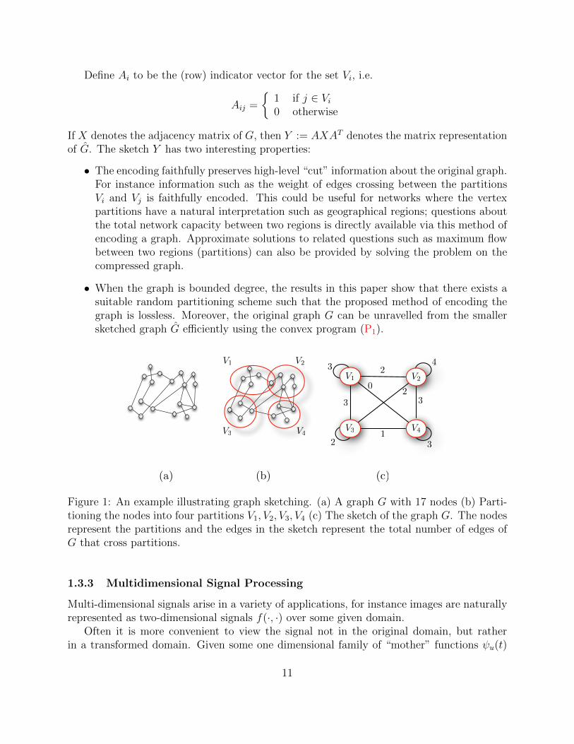
Similar to the one-dimensional case, appropriate choices of yeild standard transforms suchas the two-dimensional Fourier transform and the two-dimensional wavelet transform. Theadvantage of working with an alternate basis as described above is that signals often haveparticularly simple representations when the basis is appropriately chosen. It is well-known,for instance, that natural images have a sparse representation in the wavelet basis (see Fig.2). Indeed, many natural images are not only sparse, but they are also distributed sparse,when represented in the wavelet basis. This enables compression by performing “pooling”of wavelet coe�cients, as described below.

Figure 2: Note that the wavelet representaion of the image is distributed sparse.

In many applications, it is more convenient to work with discrete signals and their trans-forms (by discretizing the variables (t, r) and the transform domain variables (u, v)). Itis natural to represent the discretization of the two-dimensional signal f(t, r) by a ma-trix F 2 Rp⇥p. The corresponding discretization of u(t) can be represented as a matrix = [ ]ut, and the discretized version of the f(u, v), denoted by F is given by:

F = F T.

12

As noted above, in several applications of interest, when the basis is chosen appro-priately, the signal has a succinct representation and the corresponding matrix F is sparse.This is true, for instance, when F represents a natural image and F is the wavelet transformof F . Due to the sparse representability of the signal in this basis, it is possible to acquireand store the signal in a compressive manner. For instance, instead of sensing the signal Fusing (which correpsonds to sensing the signal at every value of the transform variable u),one could instead form “pools” of transform variables Si = {ui1, ui2 . . . , uik} and sense thesignal via

A =

2

64

Pu2S1

u...P

u2Sm u

3

75 ,

where the matrix A corresponds to the pooling operation. This means of compression corre-sponds to “mixing” measurements at randomly chosen transform domain values u. (When is the Fourier transform, this corresponds to randomly chosen frequencies, and when isthe wavelet, this corresponds to mixing randomly chosen translation and scale parameters). When the signal F is acquired in this manner, we obtain measurements of the form:

Y = AFA

T,

where F is suitably sparse. Note that one may choose di↵erent random mixtures of mea-surements for the t and r “spatial” variables, in which case one would obtain measurementsof the form:

Y = AFB

T.

The theory developed in this paper shows how one can recover the multi-dimensional signalF from such an undersampled acquisition mechanism. In particular, our results will showthat if the pooling of the transform variable is done suitably randomly, then there is ane�cient method based on linear programming that can be used to recover the original multi-dimensional signal.

1.4 Related Work and Obstacles to Common Approaches

The problem of recovering sparse signals via `1 regularization and convex optimization hasbeen studied extensively in the past decade; our work fits broadly into this context. Inthe signal processing community, the literature on compressed sensing [10, 20] focuses onrecovering sparse signals from data. In the statistics community, the LASSO formulation asproposed by Tibshirani, and subsequently analyzed (for variable selection) by Meinshausenand Buhlmann [39], and Wainwright [48] are also closely related. Other examples of struc-tured model selection include estimation of models with a few latent factors (leading tolow-rank covariance matrices) [23], models specified by banded or sparse covariance matrices[7, 8], and Markov or graphical models [38, 39, 42]. These ideas have been studied in depthand extended to analyze numerous other model selection problems in statistics and signalprocessing [4, 14, 12].

13

Our work is also motivated by the work on sketching in the computer science community;this literature deals with the idea of compressing high-dimensional data vectors via projectionto low-dimensions while preserving pertinent geometric properties. The celebrated Johnson-Lindenstrauss Lemma [31] is one such result, and the idea of sketching has been exploredin various contexts [2, 34]. The idea of using random bipartite graphs and their relatedexpansion properties, which motivated our approach to the problem, have also been studiedin past work [5, 35, 36].

While most of the work on sparse recovery focuses on sensing matrices where each entryis an i.i.d. random variable, there are a few lines of work that explore structured sensingmatrices. For instance, there have been studies of matrices with Toeplitz structure [28],or those with random entries with independent rows but with possibly dependent columns[47, 44]. Also related is the work on deterministic dictionaries for compressed sensing [16],although those approaches yield results that are too weak for our setup.

One interesting aspect of our work is that we show that it is possible to use highlyconstrained sensing matrices (i.e. those with tensor product structure) to recover the signal ofinterest. Many standard techniques fail in this setting. Restricted isometry based approaches[11] and coherence based approaches [18, 26, 46] fail due to a lack of independence structurein the sensing matrix. Indeed, the restricted isometry constants as well as the coherenceconstants are known to be weak for tensor product sensing operators [22, 32]. Gaussianwidth based analysis approaches [13] fail because the kernel of the sensing matrix is not auniformly random subspace and hence not amenable to a similar application of Gordon’s(“escape through the mesh”) theorem. We overcome these technical di�culties by workingdirectly with combinatorial properties of the tensor product of a random bipartite graph,and exploiting those to prove the so-called nullspace property [19, 15].

2 Experiments

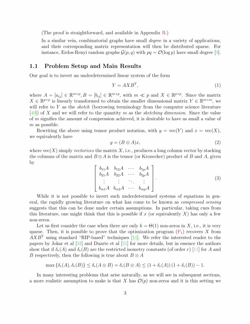
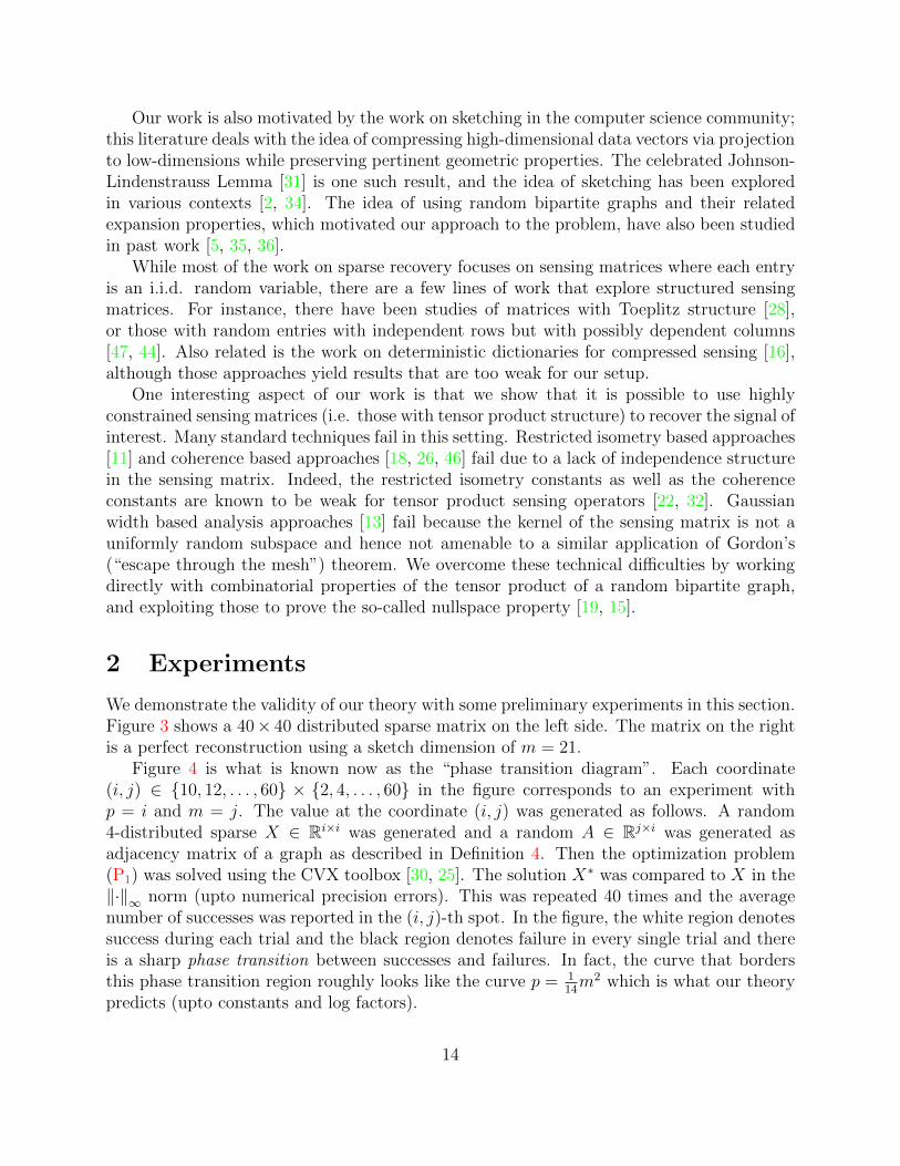
We demonstrate the validity of our theory with some preliminary experiments in this section.Figure 3 shows a 40⇥ 40 distributed sparse matrix on the left side. The matrix on the rightis a perfect reconstruction using a sketch dimension of m = 21.

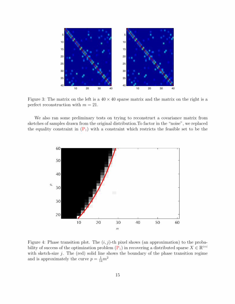
Figure 4 is what is known now as the “phase transition diagram”. Each coordinate(i, j) 2 {10, 12, . . . , 60} ⇥ {2, 4, . . . , 60} in the figure corresponds to an experiment withp = i and m = j. The value at the coordinate (i, j) was generated as follows. A random4-distributed sparse X 2 Ri⇥i was generated and a random A 2 Rj⇥i was generated asadjacency matrix of a graph as described in Definition 4. Then the optimization problem(P1) was solved using the CVX toolbox [30, 25]. The solution X

⇤ was compared to X in thek·k1 norm (upto numerical precision errors). This was repeated 40 times and the averagenumber of successes was reported in the (i, j)-th spot. In the figure, the white region denotessuccess during each trial and the black region denotes failure in every single trial and thereis a sharp phase transition between successes and failures. In fact, the curve that bordersthis phase transition region roughly looks like the curve p = 1

14m2 which is what our theory

predicts (upto constants and log factors).

14

10 20 30 40

5

10

15

20

25

30

35

4010 20 30 40

5

10

15

20

25

30

35

40

Figure 3: The matrix on the left is a 40⇥ 40 sparse matrix and the matrix on the right is aperfect reconstruction with m = 21.

We also ran some preliminary tests on trying to reconstruct a covariance matrix fromsketches of samples drawn from the original distribution.To factor in the “noise”, we replacedthe equality constraint in (P1) with a constraint which restricts the feasible set to be the

m

p

Figure 4: Phase transition plot. The (i, j)-th pixel shows (an approximation) to the proba-bility of success of the optimization problem (P1) in recovering a distributed sparse X 2 Ri⇥i

with sketch-size j. The (red) solid line shows the boundary of the phase transition regimeand is approximately the curve p = 1

14m2

15

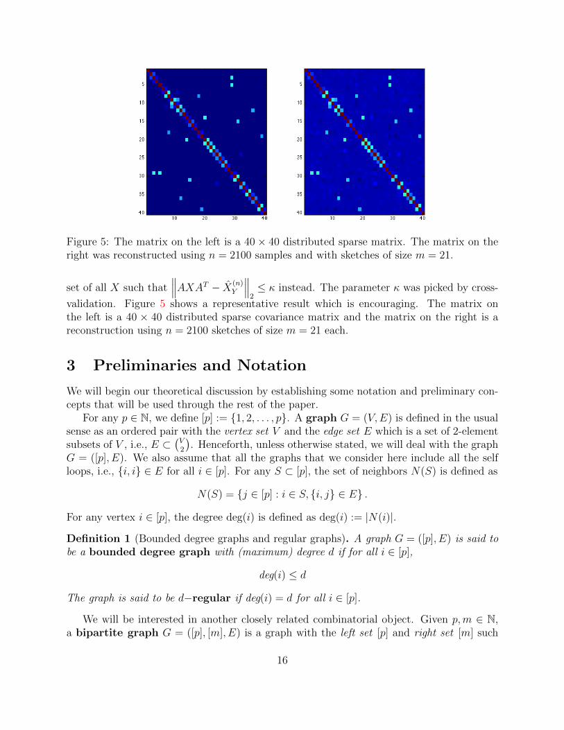
Figure 5: The matrix on the left is a 40⇥ 40 distributed sparse matrix. The matrix on theright was reconstructed using n = 2100 samples and with sketches of size m = 21.

set of all X such that���AXA

T � X

(n)Y

���2 instead. The parameter was picked by cross-

validation. Figure 5 shows a representative result which is encouraging. The matrix onthe left is a 40 ⇥ 40 distributed sparse covariance matrix and the matrix on the right is areconstruction using n = 2100 sketches of size m = 21 each.

3 Preliminaries and Notation

We will begin our theoretical discussion by establishing some notation and preliminary con-cepts that will be used through the rest of the paper.

For any p 2 N, we define [p] := {1, 2, . . . , p}. A graph G = (V,E) is defined in the usualsense as an ordered pair with the vertex set V and the edge set E which is a set of 2-elementsubsets of V , i.e., E ⇢ �V2

�. Henceforth, unless otherwise stated, we will deal with the graph

G = ([p], E). We also assume that all the graphs that we consider here include all the selfloops, i.e., {i, i} 2 E for all i 2 [p]. For any S ⇢ [p], the set of neighbors N(S) is defined as

N(S) = {j 2 [p] : i 2 S, {i, j} 2 E} .For any vertex i 2 [p], the degree deg(i) is defined as deg(i) := |N(i)|.Definition 1 (Bounded degree graphs and regular graphs). A graph G = ([p], E) is said tobe a bounded degree graph with (maximum) degree d if for all i 2 [p],

deg(i) d

The graph is said to be d�regular if deg(i) = d for all i 2 [p].

We will be interested in another closely related combinatorial object. Given p,m 2 N,a bipartite graph G = ([p], [m], E) is a graph with the left set [p] and right set [m] such

16

that the edge set E only has pairs {i, j} where i is the left set and j is in the right set. Abipartite graph G = ([p], [m], E) is said to be ��left regular if for all i in the left set [p],deg(i) = �. Given two sets A ⇢ [p], B ⇢ [m], we define the set

E (A : B) := {(i, j) 2 E : i 2 A, j 2 B} ,which we will find use for in our analysis. This set is sometimes known as the cut set. Finallyfor a set A ⇢ [p] (resp. B ⇢ [m]), we define N(A) := {j 2 [m] : i 2 A, {i, j} 2 E} (resp.NR(B) := {i 2 [p] : j 2 B, {i, j} 2 E} ). This distinction between N and NR is made onlyto reinforce the meaning of the quantities which is otherwise clear in context.

Definition 2. (Tensor graphs) Given two bipartite graphs G1 = ([p], [m], E1) and G2 =([p], [m], E2), we define their tensor graph G1⌦G2 to be the bipartite graph ([p]⇥ [p], [m]⇥[m], E1 ⌦E2) where E1 ⌦E2 is such that {(i, i0), (j, j0)} 2 E1 ⌦E2 if and only if {i, j} 2 E1

and {i0, j0} 2 E2.

Notice that if the adjacency matrices of G1, G2 are given respectively by A

T, B

T 2 Rp⇥m,then the adjacency matrix of G1 ⌦G2 is (A⌦ B)T 2 Rp2⇥m2

.As mentioned earlier, we will be particularly interested in the situation where B = A.

In this case, write the tensor product of a graph G = ([p], [m], E) with itself as G

⌦ =([p]⇥ [p], [m]⇥ [m], E⌦). Here E

⌦ is such that {(i, i0), (j, j0)} 2 E

⌦ if and only if {i, j} and{i0, j0} are in E.

Throughout this paper, we write k · k to denote norms of vectors. For instance, kxk1 andkxk2 respectively stand for the `1 and `2 norm of x. Furthermore, for a matrix X, we willoften write kXk to denote kvec(X)k to avoid clutter. Therefore, the Frobenius norm of amatrix X will appear in this paper as kXk2.

3.1 Distributed Sparsity

As promised, we will now argue that distributed sparsity is important. Towards this end, letus turn our attention to Figure 6 which shows two matrices with O(p) non-zeros. Supposethat the non-zero pattern in X looks like that of the matrix on the left (which we dub asthe “arrow” matrix). It is clear that it is impossible to recover this X from AXB

T even ifwe know the non-zero pattern in advance. For instance, if v 2 ker(A), then the matrix X,with v added to the first column of X is such that AXB

T = AXB

T and X is also an arrowmatrix and hence indistinguishable from X. Similarly, one can “hide” a kernel vector of Bin the first row of the arrow matrix. In other words, it is impossible to uniquely recover Xfrom AXB

T .In what follows, we will show that if the sparsity pattern of X is more distributed, as in

the right side of Figure 6, then one can recover X and do so e�ciently. In fact, our analysiswill also reveal what that the size of the sketch Y needs to be able to perform this task andwe will see that this is very close to being optimal.In order to make things concrete, we will now define these notions formally.

17

"Arrow" matrix Distributed sparse matrix

Figure 6: Two matrices with O(p) non-zeros. The “arrow” matrix is impossible to recoverby covariance sketching while the distributed sparse matrix is.

Definition 3 (d�distributed sets and d�distributed sparse matrices). We say that a subset⌦ ⇢ [p]⇥ [p] is d�distributed if the following hold.

1. For i = 1, 2, . . . , p, (i, i) 2 ⌦.2. For all k 2 [p], the cardinality of the sets ⌦k := {(i, j) 2 ⌦ : i = k} and ⌦k :=

{(i, j) 2 ⌦ : j = k} is no more than d.

The set of all d�distributed subsets of [p]⇥ [p] will be denoted as Wp,d. We say that a matrixX 2 Rp⇥p is d�distributed sparse if there exists an ⌦ 2 Wd,p such that supp(X) :={(i, j) 2 [p]⇥ [p] : Xij 6= 0} ⇢ ⌦.

While the theory we develop here is more generally applicable, the first point in the abovedefinition makes the presentation easier. Notice that this forces the number of o↵-diagonalnon-zeros in each row or column of a d�distributed sparse matrix X to be at most d�1. Thisis not a serious limitation since a more careful analysis along these lines can only improvethe bounds we obtain by at most a constant factor.Examples:

• Any diagonal matrix is d�distributed sparse for d = 1. Similarly a tridiagonal matrixis d�distributed sparse with d = 3.

• The adjacency matrix of a bounded degree graph with maximum degree d � 1 isd�distributed sparse

• As shown in Proposition 1, random sparse matrices are d�distributed sparse withd = O(log p). While we implicitly assume that d is constant with respect to p in whatfollows, all arguments work even if d grows logarithmically in p as is the case here.

Given a matrix X 2 Rp⇥p, as mentioned earlier, we write vec(X) to denote the Rp2

vector obtained by stacking the columns of X. Suppose x = vec(X). It will be useful inwhat follows to remember that x was actually derived from the matrix X and hence wewill employ slight abuses of notation as follows: We will say x is d�distributed sparse when

18

we actually mean that the matrix X is. Also, we will write (i, j) to denote the index of xcorresponding to Xij, i.e.,

xij := x(i�1)p+j = Xij.

We finally make two remarks:

• Even if X were distributed sparse, the observed vector Y = AXB

T is usually unstruc-tured (and dense).

• While the results in this paper focus on the regime where the maximum number ofnon-zeros d per row/column of X is a constant (with respect to p), they can be readilyextended to the case when d grows poly-logarithmically in p. Extensions to moregeneral scalings of d is an interesting avenue for future work.

3.2 Random Bipartite Graphs, Weak Distributed Expansion andthe Choice of the Sketching Matrices

As alluded to earlier, we will choose the sensing matrices A,B to be the adjacency matricesof certain random bipartite graphs. The precise definition of this notion follows.

Definition 4 (Uniformly Random ��left regular bipartite graph). We say that G = ([p], [m], E)is a uniformly random ��left regular bipartite graph if the edge set E is a random variablewith the following property: for each i 2 [p] one chooses � vertices j1, j2, . . . , j� chosen uni-formly and independently at random (with replacement) from [m] such that {{i, jk}}�k=1 ⇢ E.

Remarks:

• Note that since we are sampling with replacement, it follows that the bipartite graphthus constructed may not be simple. If for instance there are two edges from the leftnode i to the right node i, the corresponding entry Aij = 2.

• It is in fact possible to work with a sampling without replacement model in Definition 4(where the resulting graph is indeed simple) and obtain qualititatively the same results.We work with a “sampling with replacement” model for the ease of exposition.

The probabilistic claims in this paper are made with respect to this probability distributionon the space of all bipartite graphs.

In past work [5, 35], the authors show that a random graph generated as above is, forsuitable values of ✏, �, a (k, �, ✏)�expander. That is, for all sets S ⇢ [p] such that |S| k,the size of the neighborhood |N(S)| is no less than (1 � ✏)� |S|. If A is the adjacencymatrix of such a graph, then it can then be shown that this implies that `1 minimizationwould recover a k�sparse vector x if one observes the sketch Ax (actually, [5] shows thatthese two properties are equivalent). Notice that in our context, the vector that we need torecover is O(p) sparse and therefore, our random graph needs to be a (O(p), �, ✏)�expander.Unfortunately, this turns out to not be true of G1⌦G2 when G1 and G2 are randomly chosenas directed above.

19

However, we prove that if G1 and G2 are picked as in Definition 4, then their tensor graphG1⌦G2, satisfies what can be considered a weak distributed expansion property. This roughlysays that the neighborhood of a d�distributed ⌦ ⇢ [p] ⇥ [p] is large enough. Moreover, weshow that this is in fact su�cient to prove that with high probability X can be recoveredfrom AXB

T e�ciently. The precise statement of these combinatorial claims follows.

Lemma 1. Suppose that G1 = ([p], [m], E1) and G2 = ([p], [m], E2) are two independentuniformly random ��left regular bipartite graphs with � = O(log p) and m = O(

pdp log p).

Let ⌦ 2 Wd,p be fixed. Then there exists an ✏ 2 �0, 14�such that G1 ⌦ G2 has the following

properties with probability exceeding 1� p

�c, for some c > 0.

1. |N(⌦)| � p�

2(1� ✏).

2. For any (i, i0) 2 ([p]⇥ [p]) \ ⌦ we have |N(i, i0) \N(⌦)| ✏�

2.

3. For any (i, i0) 2 ⌦, |N(i, i0) \N(⌦ \ (i, i0))| ✏�

2.

Moreover, all these claims continue to hold when G2 is the same as G1.

Remarks:

• Part 1 of Lemma 1 says that if ⌦ is a d�distributed set, then the size of the neghborhoodof ⌦ is large. This can be considered a weak distributed expansion property. Noticethat while it is reminiscent of the vertex expansion property of expander graphs, it iseasy to see that it does not hold if ⌦ is not distributed. Furthermore, we call it “weak”because the lower bound on the size of the neighborhood is �2p(1 � ✏) as opposed to�

2 |⌦| (1 � ✏) = �

2dp(1 � ✏) as one typically gets for standard expander graphs. It

will become clear that this is one of the key combinatorial facts that ensures that thenecessary theoretical guarantees hold for covariance sketching.

• Parts 2 and 3 say that the number of collisions between the edges emanating out of asingle vertex with the edges emanating out of a distributed set is small. Again, thiscombinatorial property is crucial for the proof of Theorem 1 to work.

As stated earlier, we are particularly interested in the challenging case when G1 = G2 (orequivalently, their adjacency matrices A,B are the same). The di�cultly, loosely speaking,stems from the fact that since we are not allowed to pick G1 and G2 separately, we havemuch less independence. In Appendix A, we will only prove Lemma 1 in the case whenG1 = G2 since this proof can be modified in a straightforward manner to obtain the proofof the case when G1 and G2 are drawn independently.

4 Proofs of Main Results

In this section, we will prove the main theorem. To reduce clutter in our presentation, wewill sometimes employ certain notational shortcuts. When the context is clear, the ordered

20

pair (i, i0) will simply be written as ii0 and the set [p]⇥ [p] will be written as [p]2. Sometimes,we will also write A to mean A⌦ A and if S ⇢ [p]⇥ [p], we write (A⌦ A)S or AS to meanthe submatrix of A⌦ A obtained by appending the columns {Ai ⌦ Aj | (i, j) 2 S}.

As stated earlier, we will only provide the proof of Theorem 1 for the case when A = B.Some straightforward changes to the proof presented here readily gives one the proof for thecase when the matrices A and B are distinct.

4.1 Proof of Theorem 1

We will consider an arbitrary ordering of the set [p]⇥ [p] and we will order the edges in E

⌦

lexicographically based on this ordering, i.e., the first �2 edges e1, . . . , e�2 in E

⌦ are thosethat correspond to the first element as per the ordering on [p] ⇥ [p] and so on. Now, onecan imagine that the graph G

⌦ is formed by including these edges sequentially as per theordering on the edges. This allows us to partition the edge set into the set E⌦

1 of edges thatdo not collide with any of the previous edges as per the ordering and the set E⌦

2 := E

⌦�E

⌦1 .

(We note that a similar proof technique was adopted in Berinde et al. [5]).As a first step towards proving the main theorem, we will show that the operator A⌦A

preserves the `1 norm of a matrix X as long as X is distributed sparse. Berinde et al.,[5] calla similar property RIP-1, taking cues from the restricted isometry property that has becomepopular in literature [11]. The proposition below can also be considered to be a restrictedisometry property but the operator in our case is only constrained to behave like an isometryfor distributed sparse vectors.

Proposition 2 (`1-RIP). Suppose X 2 Rp⇥p is d�distributed sparse and A is the adjacencymatrix of a random bipartite ��left regular graph. Then there exists an ✏ > 0 such that

(1� 2✏)�2 kXk1 ��AXA

T��1 �

2 kXk1 , (6)

with probability exceeding 1� p

�c for some c > 0.

Proof. The upper bound follows (deterministically) from the fact that the induced (matrix)`1-norm of A ⌦ A, i.e., the maximum column sum of A ⌦ A, is precisely �2. To prove thelower bound, we need the following lemma.

Lemma 2. For any X 2 Rp⇥p,

��AXA

T��1� �

2 kXk1 � 2X

jj02[m]2

X

ii02[p]21{ii0,jj0}2E⌦

2|Xii0 | (7)

Proof. In what follows, we will denote the indicator function 1{ii0,jj0}2S by 1{ii0jj0}S . We begin

21

by observing that

��AXA

T��1= kA vec(X)k1

=X

jj02[m]2

������

X

ii02[p]2A{ii0jj0}Xii0

������

=X

jj02[m]2

������

X

ii02[p]21{ii0jj0}E⌦ Xii0

������

=X

jj02[m]2

������

X

ii02[p]21{ii0jj0}E⌦

1Xii0 +

X

ii02[p]21{ii0jj0}E⌦

2Xii0

������

�X

jj02[m]2

������

X

ii02[p]21{ii0jj0}E⌦

1Xii0

�������������

X

ii02[p]21{ii0jj0}E⌦

2Xii0

������(a)

�X

jj02[m]2

⇣ X

ii02[p]21{ii0jj0}E⌦

1|Xii0 |�

X

ii02[p]21{ii0jj0}E⌦

2|Xii0 |

⌘

=X

ii02[p]2,jj02[m]2

1{ii0jj0}E⌦ |Xii0 |� 2

X

ii02[p]2jj02[m]2

1{ii0jj0}E⌦

2|Xii0 | ,

where (a) follows after observing that the first (double) sum has only one term and applyingtriangle inequality to the second sum. SinceP

ii02[p]2,jj02[m]2 1{ii0jj0}E⌦ |Xii0 | = �

2 kXk1, this concludes the proof of the lemma.

Now, to complete the proof of Proposition 2, we need to bound the sum in the LHS of(7). Notice that X

ii0jj0:(ii0jj0)2E⌦2

|Xii0 | =X

ii0

|Xii0 | rii0 =X

ii02⌦

|Xii0 | rii0 .

where rii0 is the number of collisions of edges emanating from ii

0 with all the previous edgesas per the ordering we defined earlier. Since ⌦ is d�distributed, from the third part ofLemma 1, we have that for all ii0 2 ⌦, rii0 ✏�

2 with probability exceeding 1 � p

�c andtherefore, X

ii02⌦

|Xii0 | rii0 ✏�

2 kXk1 .

This concludes the proof.

Next, we will use the fact that A ⌦ A behaves as an approximate isometry (in the `1norm) to prove what can be considered a nullspace property [19, 15]. This will tell us thatthe nullspace of A ⌦ A is “smooth” with respect to distributed support sets and hence `1minimization as proposed in (P1) will find the right solution.

22

Proposition 3 (Nullspace Property). Suppose that A 2 {0, 1}m⇥p is the adjacency matrixof a random bipartite ��left regular graph with � = O(log p) and m = O(

pdp log p) and that

⌦ 2 Wd,p is fixed. Then, with probability exceeding 1 � p

�c, for any V 2 Rp⇥p such thatAV A

T = 0, we have

kV⌦k1 ✏

1� 3✏kV⌦ck1 . (8)

for some ✏ 2 (0, 14) and for some c > 0.

Proof. Let V be any symmetric matrix such that AV A

T = 0. Let v = vec(V) and note thatvec�AV A

T�= (A⌦ A) v = 0. Let ⌦ be a d-distributed set. As indicated in Section 3,

we define N(⌦) ✓ [m]2 to be the set of neighbors of ⌦ with respect to the graph G

⌦. Let(A ⌦ A)N(⌦) denote the submatrix of A ⌦ A that contains only those rows correspondingto N(⌦) (and all columns). We will slightly abuse notation and use v⌦ to denote thevectorization of the projection of V onto the set ⌦, i.e., v⌦ = vec(V⌦), where

[V⌦]i,j =

(Vi,j (i, j) 2 ⌦0 otherwise

.

Now, we can follow the following chain of inequalities:

0 =��(A⌦ A)N(⌦)

v

��1

=��(A⌦ A)N(⌦)(v⌦ + v⌦c)

��1

� ��(A⌦ A)N(⌦)v⌦

��1� ��(A⌦ A)N(⌦)

v⌦c

��1

= k(A⌦ A)v⌦k1 ���(A⌦ A)N(⌦)

v⌦c

��1

� (1� 2✏)�2 kV⌦k1 ���(A⌦ A)N(⌦)

v⌦c

��1,

where the last inequality follows from Proposition 2. Resuming the chain of inequalities, wehave:

0 � (1� 2✏)�2 kV⌦k1 �X

ii02⌦c

��(A⌦ A)N(⌦)v{ii0}

��1

� (1� 2✏)�2 kV⌦k1 �X

ii0,jj0:(ii0,jj0)2E⌦,jj02N(⌦),ii02⌦c

|Vii0 |

= (1� 2✏)�2 kV⌦k1 �X

ii02⌦c

|E⌦(ii0 : N(⌦))| |Vii0 |

(a)

� (1� 2✏)�2 kV⌦k1 �X

ii02⌦c

✏�

2 |Vii0 |

� (1� 2✏)�2 kV⌦k1 � ✏�

2 kV k1 ,where (a) follows from the second part of Lemma 1. Writing kV k1 = kV⌦k1 + kV⌦ck1 andrearranging, we get the required result.

23

Now, we can use this to prove our main theorem.

Proof of Theorem 1. Let ⌦ be the support of X and notice that ⌦ is d�distributed. Now,

suppose that there exists an X 6= X such that AXA

T = Y . Observe that A⇣X �X

⌘A

T =

0. Now, consider

kXk1 ���X � X⌦

���1+���X⌦

���1

=���⇣X � X

⌘

⌦

���1+���X⌦

���1

(a)

✏

1� 3✏

���⇣X � X

⌘

⌦c

���+���X⌦

���1

=✏

1� 3✏

����X⌦c

���+���X⌦

���1

<

���X���1

where (a) follows from Proposition 3, and the last line follows from the fact that ✏ < 14 , again

from Proposition 3. Therefore, the unique solution of (P1) is X with probability exceeding1� p

�c, for some c > 0.

5 Conclusions

In this paper we have introduced the notion of distributed sparsity for matrices. We haveshown that when a matrix is X distributed sparse, and A,B are suitable random binarymatrices, then it is possible to recover X from under-determined linear measurements of theform Y = AXB

T via `1 minimization. We have also shown that this recovery procedure isrobust in the sense that if X is equal to a distributed sparse matrix plus a perturbation,then our procedure returns an approximation with accuracy proportional to the size of theperturbation. Our results follow from a new lemma about the properties of tensor productsof random bipartite graphs. We also describe three interesting applications where our resultswould be directly applicable.

In future work, we plan to investigate the statistical behavior and sample complexityof estimating a distributed sparse matrix (and its exact support) in the presence of vari-ous sources of noise (such as additive Gaussian noise, and Wishart noise). We expect aninteresting trade-o↵ between the sketching dimension and the sample complexity.

References

[1] Kook Jin Ahn, Sudipto Guha, and Andrew McGregor. Graph sketches: sparsifica-tion, spanners, and subgraphs. In Proceedings of the 31st symposium on Principles ofDatabase Systems, pages 5–14. ACM, 2012.

24

[2] Alexandr Andoni, Khanh Do Ba, Piotr Indyk, and David Woodru↵. E�cient sketchesfor earth-mover distance, with applications. In in FOCS, 2009.

[3] Dana Angluin and Leslie G. Valiant. Fast probabilistic algorithms for hamiltoniancircuits and matchings. Journal of Computer and system Sciences, 18(2):155–193, 1979.

[4] L. Balzano, R. Nowak, and B. Recht. Online identification and tracking of subspacesfrom highly incomplete information. In Proceedings of the 48th Annual Allerton Con-ference, 2010.

[5] R. Berinde, A.C. Gilbert, P. Indyk, H. Karlo↵, and M.J. Strauss. Combining geometryand combinatorics: A unified approach to sparse signal recovery. In Communication,Control, and Computing, 2008 46th Annual Allerton Conference on, pages 798 –805,sept. 2008.

[6] Dimitris Bertsimas and John N Tsitsiklis. Introduction to linear optimization. AthenaScientific Belmont, MA, 1997.

[7] P. J. Bickel and E. Levina. Covariance regularization by thresholding. Annals of Statis-tics, 36(6):2577–2604, 2008.

[8] P. J. Bickel and E. Levina. Regularized estimation of large covariance matrices. Annalsof Statistics, 36(1):199–227, 2008.

[9] B. Bollobas. Random graphs, volume 73. Cambridge university press, 2001.

[10] E.J. Candes, J. Romberg, and T. Tao. Robust uncertainty principles: Exact signal re-construction from highly incomplete frequency information. Information Theory, IEEETransactions on, 52(2):489–509, 2006.

[11] E.J. Candes and T. Tao. Decoding by linear programming. Information Theory, IEEETransactions on, 51(12):4203–4215, 2005.

[12] Emmanuel J Candes, Xiaodong Li, Yi Ma, and John Wright. Robust principal compo-nent analysis? arXiv preprint arXiv:0912.3599, 2009.

[13] V. Chandrasekaran, B. Recht, P. A. Parrilo, and A. S. Willsky. The Convex Geometryof Linear Inverse Problems. ArXiv e-prints, December 2010.

[14] Venkat Chandrasekaran, Benjamin Recht, PabloA. Parrilo, and AlanS. Willsky. Theconvex geometry of linear inverse problems. Foundations of Computational Mathemat-ics, 12:805–849, 2012.

[15] Albert Cohen, Wolfgang Dahmen, and Ronald Devore. COMPRESSED SENSING ANDBEST k-TERM APPROXIMATION. Journal of the American Mathematical Society,22(1):211–231, 2009.

25

[16] Graham Cormode and S Muthukrishnan. Combinatorial algorithms for compressedsensing. Structural Information and Communication Complexity, pages 280–294, 2006.

[17] Peter J Diggle and Arunas P Verbyla. Nonparametric estimation of covariance structurein longitudinal data. Biometrics, pages 401–415, 1998.

[18] David L Donoho and Michael Elad. Optimally sparse representation in general(nonorthogonal) dictionaries via ?1 minimization. Proceedings of the National Academyof Sciences, 100(5):2197–2202, 2003.

[19] David L Donoho and Xiaoming Huo. Uncertaintly Principles and Ideal Atomic Decom-position. IEEE Transactions on Information Theory, 47(7):2845–2862, 2001.

[20] David Leigh Donoho. Compressed sensing. Information Theory, IEEE Transactions on,52(4):1289–1306, 2006.

[21] Marco F Duarte and Richard G Baraniuk. Kronecker compressive sensing. ImageProcessing, IEEE Transactions on, 21(2):494–504, 2012.

[22] M.F. Duarte and R.G. Baraniuk. Kronecker product matrices for compressive sensing. InAcoustics Speech and Signal Processing (ICASSP), 2010 IEEE International Conferenceon, pages 3650 –3653, march 2010.

[23] J. Fan, Y. Fan, and J. Lv. High dimensional covariance matrix estimation using a factormodel. Journal of Econometrics, 147(1):43, 2007.

[24] Anna C Gilbert and Kirill Levchenko. Compressing network graphs. In Proceedings ofthe LinkKDD workshop at the 10th ACM Conference on KDD. Citeseer, 2004.

[25] M. Grant and S. Boyd. Graph implementations for nonsmooth convex programs. InV. Blondel, S. Boyd, and H. Kimura, editors, Recent Advances in Learning and Con-trol, Lecture Notes in Control and Information Sciences, pages 95–110. Springer-VerlagLimited, 2008.

[26] Remi Gribonval and Morten Nielsen. Sparse representations in unions of bases. Infor-mation Theory, IEEE Transactions on, 49(12):3320–3325, 2003.

[27] Andras Hajnal and Endre Szemeredi. Proof of a conjecture of erdos. Combinatorialtheory and its applications, 2:601–623, 1970.

[28] Jarvis Haupt, Waheed U Bajwa, Gil Raz, and Robert Nowak. Toeplitz compressedsensing matrices with applications to sparse channel estimation. Information Theory,IEEE Transactions on, 56(11):5862–5875, 2010.

[29] Larry V Hedges, Ingram Olkin, Mathematischer Statistiker, Ingram Olkin, and IngramOlkin. Statistical methods for meta-analysis. Academic Press New York, 1985.

26

[30] CVX Research, Inc. CVX: Matlab software for disciplined convex programming, version2.0 beta, September 2012.

[31] W.B. Johnson and J. Lindenstrauss. Extensions of Lipschitz mappings into a Hilbertspace. Contemporary mathematics, 26(189-206):1–1, 1984.

[32] S. Jokar. Sparse recovery and kronecker products. In Information Sciences and Systems(CISS), 2010 44th Annual Conference on, pages 1 –4, march 2010.

[33] Sadegh Jokar and Volker Mehrmann. Sparse solutions to underdetermined kroneckerproduct systems. Linear Algebra and its Applications, 431(12):2437–2447, 2009.

[34] Daniel M. Kane, Jelani Nelson, Ely Porat, and David P. Woodru↵. Fast momentestimation in data streams in optimal space. In Proceedings of the 43rd annual ACMsymposium on Theory of computing, STOC ’11, pages 745–754, New York, NY, USA,2011. ACM.

[35] M. Amin Khajehnejad, Alexandros G. Dimakis, Weiyu Xu, and Babak Hassibi. Sparserecovery of positive signals with minimal expansion. CoRR, abs/0902.4045, 2009.

[36] MAmin Khajehnejad, Alexandros G Dimakis, Weiyu Xu, and Babak Hassibi. Sparserecovery of nonnegative signals with minimal expansion. Signal Processing, IEEE Trans-actions on, 59(1):196–208, 2011.

[37] H. A. Kierstead and A. V. Kostochka. A short proof of the Hajnal-Szemeredi Theoremon equitable colouring. Comb. Probab. Comput., 17(2):265–270, March 2008.

[38] S. Lauritzen. Graphical Models. Clarendon Press, Oxford, 1996.

[39] Nicolai Meinshausen and Peter Buhlmann. High-dimensional graphs and variable selec-tion with the lasso. The Annals of Statistics, 34(3):1436–1462, 2006.

[40] S Muthukrishnan. Data streams: Algorithms and applications. Now Publishers Inc,2005.

[41] Sriram V. Pemmaraju. Equitable colorings extend Cherno↵-Hoe↵ding bounds. In Pro-ceedings of the twelfth annual ACM-SIAM symposium on Discrete algorithms, SODA’01, pages 924–925, Philadelphia, PA, USA, 2001. Society for Industrial and AppliedMathematics.

[42] P. Ravikumar, M. J. Wainwright, G. Raskutti, and B. Yu. High-dimensional covarianceestimation by minimizing `1-penalized log-determinant divergence. Electronic Journalof Statistics, 5, 2011.

[43] Adam J Rothman, Elizaveta Levina, and Ji Zhu. Generalized thresholding of largecovariance matrices. Journal of the American Statistical Association, 104(485):177–186,2009.

27

[44] Mark Rudelson and Roman Vershynin. On sparse reconstruction from fourier and gaus-sian measurements. Communications on Pure and Applied Mathematics, 61(8):1025–1045, 2008.

[45] Karen Sachs, Omar Perez, Dana Pe’er, Douglas A Lau↵enburger, and Garry P Nolan.Causal protein-signaling networks derived from multiparameter single-cell data. ScienceSignalling, 308(5721):523, 2005.

[46] Joel A Tropp. Greed is good: Algorithmic results for sparse approximation. InformationTheory, IEEE Transactions on, 50(10):2231–2242, 2004.

[47] Roman Vershynin. Introduction to the non-asymptotic analysis of random matrices.arXiv preprint arXiv:1011.3027, 2010.

[48] Martin J Wainwright. Sharp thresholds for high-dimensional and noisy sparsity recov-ery using `1�constrained quadratic programming (lasso). Information Theory, IEEETransactions on, 55(5):2183–2202, 2009.

Appendix A

Proof of Lemma 1

Lemma 1. Suppose that G1 = ([p], [m], E1) and G2 = ([p], [m], E2) are two independentuniformly random ��left regular bipartite graphs with � = O(log p) and m = O(

pdp log p).

Let ⌦ 2 Wd,p be fixed. Then there exists an ✏ 2 �0, 14�such that G1 ⌦ G2 has the following

properties with probability exceeding 1� p

�c, for some c > 0.

1. |N(⌦)| � p�

2(1� ✏).

2. For any (i, i0) 2 ([p]⇥ [p]) \ ⌦ we have |N(i, i0) \N(⌦)| ✏�

2.

3. For any (i, i0) 2 ⌦, |N(i, i0) \N(⌦ \ (i, i0))| ✏�

2.

Moreover, all these claims continue to hold when G2 is the same as G1.

Proof. As stated earlier, we will only prove this lemma for the case when G1 = G2. With afew minor modifications, one can readily get a proof for the easier case when G1 and G2 aredrawn independently.

Let E1, E2 and, E3 respectively denote the events that the implications (1), (2) and, (3)are true. Notice that

P (Ec1 [ Ec

2 [ Ec3) P(Ec

1) + P(Ec2) + P(Ec

3)

= P(Ec1) + P(Ec

2 | E1)P(E1) + P(Ec2 | Ec

1)P(Ec1)

+ P(Ec3 | E1)P(E1) + P(Ec

3 | Ec1)P(Ec

1)

3P(Ec1) + P(Ec

2 | E1) + P(Ec3 | E1)

28

Our strategy will be to upper bound P(Ec1),P(Ec

2 | E1) and, P(Ec3 | E1). Suppose the

bounds were p1, p2 and, p3 respectively, then it is easy to see that

P {E1 \ E2 \ E3} � 1�max{3p1, p2, p3}. (9)

Part 1. We will first show that P(Ec1) is small. Since ⌦ is d�distributed, the “diagonal” set

D := {(1, 1), . . . , (p, p)} is a subset of ⌦. Now, notice that for j 6= j

0 2 [m], i 2 [p],

P [(j, j0) 2 N((i, i))] =�(� � 1)

m(m� 1)(10)

This implies that

P [(j, j0) /2 N(D)] =

✓1� �(� � 1)

m(m� 1)

◆|D|

Therefore, we can bound the expected value of |N(⌦)| as follows.

E⇥ |N(⌦)| ⇤ � E

⇥ |N (D)| ⇤

=X

jj02[m]⇥[m]

P [(j, j0) 2 N(D)]

�X

jj02[m]⇥[m],j 6=j0

P [(j, j0) 2 N(D)]

=X

jj02[m]⇥[m],j 6=j0

1�

✓1� �(� � 1)

m(m� 1)

◆|D|!

= m(m� 1)

1�

✓1� �(� � 1)

m(m� 1)

◆|D|!

� m(m� 1)

|D| �(� � 1)

m(m� 1)� |D|2 �2(� � 1)2

m

2(m� 1)2

!

= |D| �2✓1�

✓1

�

+(� � 1)2 |D|m(m� 1)

◆◆

= p�

2 (1� ✏

0) .

Where in the last step, we set ✏0 = 1� +

(��1)2|D|m(m�1) .

To complete the proof, we must show that the random quantity |N(⌦)| cannot be muchsmaller than p�

2(1� ✏

0). As a first step, we define the random variables �jj0 := 1{(j,j0)2N(D)}and notice that the following chain of inequalities hold

|N(⌦)| � |N(D)| �X

jj02[m]⇥[m]j 6=j0

�jj0 .

29

Therefore, we have that

P⇥|N(⌦)| < p�

2(1� ✏

0 � ✏

00)⇤ P

2

664X

jj02[m]⇥[m]j 6=j0

�jj0 < p�

2(1� ✏

0 � ✏

00)

3

775 .

Also, since by above, EhP

j 6=j0 �jj0

i� p�

2(1� ✏

0), we have that

P⇥|N(⌦)| < p�

2(1� ✏)⇤ P

2

664X

jj02[m]⇥[m]j 6=j0

�jj0 < E

2

664X

jj02[m]⇥[m]j 6=j0

�jj0

3

775� p�

2✏

00

3

775 .

Now, notice that the sumP

j 6=j0 �jj0 has m(m � 1) terms and each term in the sum isdependent on no more than 2m�4 terms. Therefore, one way to bound the required quantityis to extract independent sub-sums from the above sum and bound the deviation of each ofthose from their means (which is the corresponding sub-sum of the mean). A principled wayof doing this is suggested by the celebrated Hajnal-Szemeridi theorem [27, 37]. Considera graph on the vertex set [m] ⇥ [m] \ {(1, 1), . . . , (m,m)} where there is an edge betweenvertices (j, j0) and (j1, j01) if j = j1 and/or j0 = j

01, i.e., exactly when the random variables

�jj0 and �j1j01are dependent. Since this graph has degree ⇥(m), Hajnal-Szemeridi theorem

tells us that this graph can be equitable colored with ⇥(m) colors. In other words, the abovesum can be partitioned into ⇥(m) sub-sums such that each sub-sum has ⇥(m) elements andthe random variables in each of them are independent. Along with this and the fact thatm(m� 1) > p�

2, we can use the union bound and write

P

2

664X

jj02[m]⇥[m]j 6=j0

�jj0 < E

2

664X

jj02[m]⇥[m]j 6=j0

�jj0

3

775� p�

2✏

00

3

775

⇥(m) P"

1

|C1|X

jj02C1

�jj0 < E"

1

|C1|X

jj02C1

�jj0

#� ✏

00

#,

where C1 is one of the “colors”. Notice that |C1| = ⇥(m).Finally, using Cherno↵ bounds, we have

⇥(m) P"

1

|C1|X

jj02C1

�jj0 <1

|C1|E"X

jj02C1

�jj0

#� ✏

00

#

⇥(m) exp��2✏002⇥(m)

.

Finally, since ✏0 can be made as small as possible, setting ✏ := ✏

0 + ✏

00 yeilds p1 < p

�c1 forsome c1 > 0. This technique of generating large deviation bounds when one has limiteddependence is not new, see [41].

30

Part 2: Now, we bound P(Ec2 | E1). Associated to a fixed i one can imagine � independent

random trials that determine the outgoing edges from i. In a similar way there are � inde-pendent random trials associated to the outgoing edges of i0. Let us fix (i, i0) and investigatethe outgoing edge (in the tensor graph) determined by the first trial of i and the first trial ofi

0. The probability that this edge emanating from the vertex (i, i0) 2 [p]2 \ {(1, 1), . . . , (p, p)}hits an arbitrary vertex (j, j0) 2 [m]2 is given by 1/m2. The probability that this edge landsin N(⌦) is, therefore, given by |N(⌦)| /m2. Since there are �2 edges that are incident on(i, i0), the expected size of overlap between N(i, i0) and N(⌦) is upper bounded by

�

2 |N(⌦)|m

2.

Again, to show concentration, we employ similar arguments as before and define indicatorrandom variables �1 . . . ,��2 each of which corresponds to one of the edges emanating fromthe vertex (i, i0) and then observing that the sum

P�2

k=1 �k is precisely equal to the randomquantity |N(i, i0) \N(⌦)|. To conclude that this random quantity concentrates, we firstobserve that, as above, the �2 dependent terms can be divided up into ⇥(�) with ⇥(�)elements each such that in each set the terms are independent. Therefore, we have

P|N(i, i0) \N(⌦)| > �

2 |N(⌦)|m

2(1 + ✏

0)

�= P

"�2X

k=1

�k > �

2 |N(⌦)|m

2(1 + ✏

0)

#

⇥(�) P"X

k2C1

�k > ⇥(�)|N(⌦)|m

2(1 + ✏

0)

#

⇥(�) exp⇢�� |N(⌦)|

m

2✏

0�,

where C1 is one of the colors.Therefore, since conditioned on E1, |N(⌦)| > �

2p(1 � ✏) if we pick m = �

pdp, and

� = ⇥(log p) there is a c

02 = c

02(✏

0) > 2 such that, |N(i, i0) \N(⌦)| > �

2 |N(⌦)|m2 (1 + ✏

0), withprobability not exceeding p

�c02 . Setting ✏ = (1+ ✏0) |N(⌦)| /m2, picking m as prescribed, andtaking union bound over (i, i0) 2 ⌦c, we get p2 p

�c2 for some c2 > 0.Part 3: Next, we bound P(Ec

3 | E1). Notice that the proof is very similar to that of part 2when i 6= i

0. So, here we will consider the quantity |N(i, i) \N(⌦ \ {(i, i)})|.As explained above to each left node i we associate � random trials that determine its

outgoing edges. Correspondingly, if we fix a left node (i, i) in the tensor graph, and thinkof its outgoing edges they are determined by the outcome of �2 product trials. Let 1k(j) bethe indicator function of the event that in the k

th trial of i the outgoing edge is incident onj. The probability that the edge associated to the (k, l) trial associated to (i, i) is incidenton (j, j0) is the random variable 1k(j)1l(j0). Note that 1k(j)1k(j0) = 1k(j) if j = j

0 and 0otherwise.

31

Note that

|N(i, i) \N(⌦ \ (i, i))| =�X

k=1

�X

l=1

X

(j,j0)2N(⌦\(i,i))

1k(j)1l(j0)

� +X

k 6=l

X

(j,j0)2N(⌦\(i,i))

1k(j)1l(j0)

When k 6= l, the trials corresponding to 1k(j),1l(j0) are independent, and hence E1k(j)1l(j0) =1m2 . We define �k,l :=

P(j,j0)2N(⌦\(i,i)) 1k(j)1l(j0) and note that E (�k,l) =

N(⌦\(i,i))m2 . We also

note that �k,l is binary valued, and

|N(i, i) \N(⌦ \ (i, i))| � +X

k 6=l

�k,l.

Therefore,

E (|N(i, i) \N(⌦ \ (i, i))|) � + (�2 � �)N(⌦ \ (i, i))

m

2

� + (�2 � �)�

2dp

m

2

�

2

✓1

�

+

✓1� 1

�

◆�

2dp

m

2

◆

�

2✏.

Next we need to prove that the quantity of interestP

k 6=l �k,l concentrates about itsmean. To that end we note that these binary valued variables are such that any particular�k,l is dependent on at most 2� � 2 other variables. Using Cherno↵ concentration boundsin conjunction with the Hajnal-Szemeredi based coloring argument explained in part 1 ofthis proof, followed by a union bound over i 2 [p] we obtain the required probability boundsp3 < p

�c3 for some c3 > 0.Substituting the bounds for p1, p2, p3 back into (9) concludes the proof.

Appendix B

Proof of Proposition 1

Proposition 1. Consider a random matrix X 2 Rp⇥p such that Xijiid⇠ Ber(�) where p� =

� = ⇥(1), then for any ✏ > 0, X is d�distributed sparse with probability at least 1�✏, where

d = �

✓1 +

2 log(2p/✏)

�

◆.

32

Proof. LetXi, i = 1, . . . , p denote the sparsity of the i�th column and letXi, i = p+1, . . . , 2p,denote the sparsity of the i�th row. Notice that the 2p random variables X1, X2, . . . , X2p are(dependent) Bin(p, �) random variables. With the choice of d as indicated in the theorem,we have the following,

P(X1 > d) = P✓X1 > �

✓1 +

log(2p/✏)

�

◆◆

(a)

exp

⇢� �

2�

2 + �

�, � =

2 log(2p/✏)

�(b)

exp

⇢���

2

�

=✏

2p

where (a) follows from the multiplicative form of the Cherno↵ Bound [3] and (b) follows aslong as � > 2. The rest of the proof follows from a simple application of the union bound.

Appendix C

Proof of Theorem 2

Theorem 2. Suppose that X is a p ⇥ p matrix. Furthermore, suppose that the hypothesesof Theorem 1 hold and let X⇤ be the solution to the optimization program (P1). Then, thereexists a c > 0 and an ✏ 2 (0, 1/4) such that the following holds with probability exceeding1� p

�c.

kX⇤ �Xk1 2� 4✏

1� 4✏

✓min

⌦2Wd,p

kX �X⌦k1◆. (11)

Proof. Since X

⇤ is the optimum of the optimization program (P1), we have that kXk1 �kX⇤k1. Let ⌦⇤ be such that kX �X⌦⇤k1 = min⌦2Wd,p

kX �XXk. We can proceed as follows

kXk1 � kX⇤k1 (12)

= k(X +X

⇤ �X)⌦k1 + k(X +X

⇤ �X)⌦ck1 (13)

� kX⌦k1 � k(X⇤ �X)⌦k1 + k(X⇤ �X)⌦ck1 � kX⌦ck1 (14)

= kXk1 � 2 kX⌦ck1 + kX⇤ �Xk1 � 2 k(X �X

⇤)⌦k1 (15)

� kXk1 � 2 kX⌦ck1 +✓1� 2✏

1� 2✏

◆kX⇤ �Xk1 (16)

where in the last step, we have used the fact that since X

⇤ is a feasible point in (P1),AX

⇤B

T = AXB

T and therefore, we can apply the result of Proposition 3 to X

⇤ �X. Thiscompletes the proof.

33