Dilute Fermi and Bose Gases

Subir Sachdev

Abstract We give a unified perspective on the properties of a variety of quantumliquids using the theory of quantum phase transitions. A central role is played by azero density quantum critical point which is argued to control the properties of thedilute gas. An exact renormalization group analysis of such quantum critical pointsleads to a computation of the universal properties of the dilute Bose gas and thespinful Fermi gas near a Feshbach resonance.

1 Introduction

This article is adapted from Chapter 16 of Quantum Phase Transitions, 2nd edition,Cambridge University Press (forthcoming).

It is not conventional to think of dilute quantum liquids as being in the vicin-ity of a quantum phase transition. However, there is a simple sense in which theyare, although there is often no broken symmetry or order parameter associated withthis quantum phase transition. We shall show below that the perspective of such aquantum phase transition allows a unified and efficient description of the universalproperties of quantum liquids.

Stated most generally, consider a quantum liquid with a global U(1) symmetry.We shall be particularly interested in the behavior of the conserved density, gener-ically denoted by Q (usually the particle number), associated with this symmetry.The quantum phase transition is between two phases with a specific T = 0 behav-ior in the expectation value of Q. In one of the phases, 〈Q〉 is pinned precisely at aquantized value (often zero) and does not vary as microscopic parameters are var-ied. This quantization ends at the quantum critical point with a discontinuity in thederivative of 〈Q〉 with respect to the tuning parameter (usually the chemical poten-

Subir SachdevDepartment of Physics, Harvard University, Cambridge MA 02138, USAe-mail: sachdev@physics.harvard.edu

1

2 Subir Sachdev

tial), and 〈Q〉 varies smoothly in the other phase; there is no discontinuity in thevalue of 〈Q〉, however.

The most familiar model exhibiting such a quantum phase transition is the diluteBose gas. We express its coherent state partition function, ZB, in terms of complexfield ΨB(x,τ), where x is a d-dimensional spatial co-ordinate and τ is imaginarytime:

ZB =∫

DΨB(x,τ)exp(−∫ 1/T

0dτ

∫ddxLB

),

LB = Ψ∗

B∂ΨB

∂τ+

12m|∇ΨB|2−µ|ΨB|2 +

u0

2|ΨB|4. (1)

We can identify the charge Q with the boson density Ψ ∗BΨB

〈Q〉=−∂FB

∂ µ= 〈|ΨB|2〉, (2)

with FB =−(T/V ) lnZB. The quantum critical point is precisely at µ = 0 and T = 0,and there are no fluctuation corrections to this location from the terms in LB. So atT = 0, 〈Q〉 takes the quantized value 〈Q〉= 0 for µ < 0, and 〈Q〉> 0 for µ > 0; wewill describe the nature of the onset at µ = 0 and finite-T crossovers in its vicinity.

Actually, we will begin our analysis in Section 2 by a model simpler than ZB,which displays a quantum phase transition with the same behavior in a conservedU(1) density 〈Q〉 and has many similarities in its physical properties. The model isexactly solvable and is expressed in terms of a continuum canonical spinless fermionfield ΨF ; its partition function is

ZF =∫

DΨF(x,τ)exp(−∫ 1/T

0dτ

∫ddxLF

),

LF = Ψ∗

F∂ΨF

∂τ+

12m|∇ΨF |2−µ|ΨF |2. (3)

LF is just a free field theory. Like ZB, ZF has a quantum critical point at µ = 0,T = 0 and we will discuss its properties; in particular, we will show that all possiblefermionic nonlinearities are irrelevant near it. The reader should not be misled bythe apparently trivial nature of the model in (3); using the theory of quantum phasetransitions to understand free fermions might seem like technological overkill. Wewill see that ZF exhibits crossovers that are quite similar to those near far morecomplicated quantum critical points, and observing them in this simple context leadsto considerable insight.

In general spatial dimension, d, the continuum theories ZB and ZF have differ-ent, though closely related, universal properties. However, we will argue that thequantum critical points of these theories are exactly equivalent in d = 1. We will seethat the bosonic theory ZB is strongly coupled in d = 1, and will note compellingevidence that the solvable fermionic theory ZF is its exactly universal solution inthe vicinity of the µ = 0, T = 0 quantum critical point. This equivalence extends to

Dilute Fermi and Bose Gases 3

observable operators in both theories, and allows exact computation of a number ofuniversal properties of ZB in d = 1.

Our last main topic will be a discussion of the dilute spinful Fermi gas in Sec-tion 4. This generalizes ZF to a spin S = 1/2 fermion ΨFσ , with σ =↑,↓. Now Fermistatistics do allow a contact quartic interaction, and so we have

ZFs =∫

DΨF↑(x,τ)DΨF↓(x,τ)exp(−∫ 1/T

0dτ

∫ddxLFs

),

LFs = Ψ∗

Fσ

∂ΨFσ

∂τ+

12m|∇ΨFσ |2−µ|ΨFσ |2 +u0Ψ

∗F↑Ψ

∗F↓ΨF↓ΨF↑. (4)

This theory conserves fermion number, and has a phase transition as a function ofincreasing µ from a state with fermion number 0 to a state with non-zero fermiondensity. However, unlike the above two cases of ZB and ZF , the transition is notalways at µ = 0. The problem defined in (4) has recently found remarkable ex-perimental applications in the study of ultracold gases of fermionic atoms. Theseexperiments are aslo able to tune the value of the interaction u0 over a wide range ofvalues, extended from repulsive to attractive. For the attractive case, the two-particlescattering amplitude has a Feshbach resonance where the scattering length diverges,and we obtain the unitarity limit. We will see that this Feshbach resonance plays acrucial role in the phase transition obtained by changing µ , and leads to a rich phasediagram of the so-called “unitary Fermi gas”.

Our treatment of ZFs in the experimental important case of d = 3 will showthat it defines a strongly coupled field theory in the vicinity of the Feshbach reso-nance for attractive interactions. It therefore pays to find alternative formulations ofthis regime of the unitary Fermi gas. One powerful approach is to promote the twofermion bound state to a separate canonical Bose field. This yields a model, ZFBwith both elementary fermions and bosons ; i.e. it is a combination of ZB and ZFswith interactions between the fermions and bosons. We will define ZFB in Section 4,and use it to obtain a number of experimentally relevant results for the unitary Fermigas.

Section 2 will present a thorough discussion of the universal properties of ZF .This will be followed by an analysis of ZB in Section 3, where we will use renor-malization group methods to obtain perturbative predictions for universal properties.The spinful Fermi gas will be discussed in Section 4.

2 The Dilute Spinless Fermi Gas

This section will study the properties of ZF in the vicinity of its µ = 0, T = 0quantum critical point. As ZF is a simple free field theory, all results can be obtainedexactly and are not particularly profound in themselves. Our main purpose is to showhow the results are interpreted in a scaling perspective and to obtain general lessonson the nature of crossovers at T > 0.

4 Subir Sachdev

First, let us review the basic nature of the quantum critical point at T = 0. Auseful diagnostic for this is the conserved density Q, which in the present modelwe identify as Ψ

†FΨF . As a function of the tuning parameter µ , this quantity has a

critical singularity at µ = 0:

⟨Ψ

†FΨF

⟩=

(Sd/d)(2mµ)d/2, µ > 0,

0, µ < 0,(5)

where the phase space factor Sd = 2/[Γ (d/2)(4π)d/2].We now proceed to a scaling analysis. Notice that at the quantum critical point

µ = 0, T = 0, the theory LF is invariant under the scaling transformations:

x′ = xe−`,

τ′ = τe−z`, (6)

Ψ′

F = ΨF ed`/2,

provided we make the choice of the dynamic exponent

z = 2. (7)

The parameter m is assumed to remain invariant under the rescaling, and its role issimply to ensure that the relative physical dimensions of space and time are com-patible. The transformation (6) also identifies the scaling dimension

dim[ΨF ] = d/2. (8)

Now turning on a nonzero µ , it is easy to see that µ is a relevant perturbationwith

dim[µ] = 2. (9)

There will be no other relevant perturbations at this quantum critical point, and sowe have for the correlation length exponent

ν = 1/2. (10)

We can now examine the consequences of adding interactions to LF . A contactinteraction such as

∫dx(Ψ †

F (x)ΨF(x))2 vanishes because of the fermion anticommu-tation relation. (A contact interaction is however permitted for a spin-1/2 Fermi gasand will be discussed in Section 4) The simplest allowed term for the spinless Fermigas is

L1 = λ(Ψ

†F (x,τ)∇Ψ

†F (x,τ)ΨF(x,τ)∇ΨF(x,τ)

), (11)

where λ is a coupling constant measuring the strength of the interaction. However,a simple analysis shows that

dim[λ ] =−d. (12)

Dilute Fermi and Bose Gases 5

This is negative and so λ is irrelevant and can be neglected in the computation ofuniversal crossovers near the point µ = T = 0. In particular, it will modify the result(5) only by contributions that are higher order in µ .

Turning to nonzero temperatures, we can write down scaling forms. Let us definethe fermion Green’s function

GF(x, t) =⟨ΨF(x, t)Ψ

†F (0,0)

⟩; (13)

then the scaling dimensions above imply that it satisfies

GF(x, t) = (2mT )d/2ΦGF

((2mT )1/2x,Tt,

µ

T

), (14)

where ΦGF is a fully universal scaling function. For this particularly simple theoryLF we can of course obtain the result for GF in closed form:

GF(x, t) =∫ ddk

(2π)deikx−i(k2/(2m)−µ)t

1+ e−(k2/(2m)−µ)/T, (15)

and it is easy to verify that this obeys the scaling form (14). Similarly the free energyFF has scaling dimension d + z, and we have

FF = T d/2+1ΦFF

(µ

T

)(16)

with ΦFF a universal scaling function; the explicit result is, of course,

FF =−∫ ddk

(2π)d ln(1+ e(µ−k2/(2m))/T ), (17)

which clearly obeys (16). The crossover behavior of the fermion density

〈Q〉=⟨Ψ

†FΨF

⟩=−∂FF

∂ µ(18)

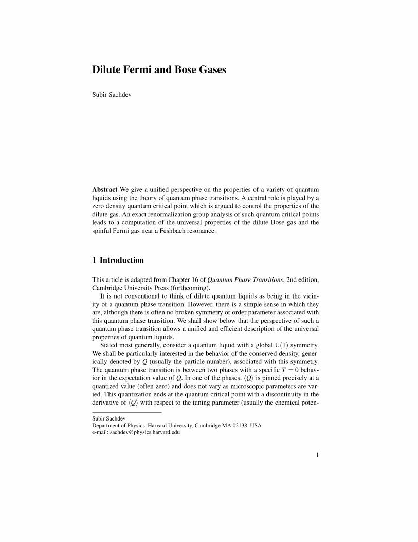
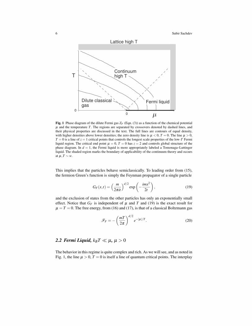
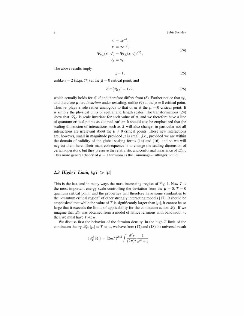
follows by taking the appropriate derivative of the free energy. Examination of theseresults leads to the crossover phase diagram of Fig. 1. We will examine each ofthe regions of the phase diagram in turn, beginning with the two low-temperatureregions.

2.1 Dilute Classical Gas, kBT |µ|, µ < 0

The ground state for µ < 0 is the vacuum with no particles. Turning on a nonzerotemperature produces particles with a small nonzero density ∼e−|µ|/T . The deBroglie wavelength of the particles is of order T−1/2, which is significantly smallerthan the mean spacing between the particles, which diverges as e|µ|/dT as T → 0.

6 Subir Sachdev

0

T

0

Lattice high T

Continuumhigh T

Fermi liquidDilute classicalgas

Fig. 1 Phase diagram of the dilute Fermi gas ZF (Eqn. (3)) as a function of the chemical potentialµ and the temperature T . The regions are separated by crossovers denoted by dashed lines, andtheir physical properties are discussed in the text. The full lines are contours of equal density,with higher densities above lower densities; the zero density line is µ < 0, T = 0. The line µ > 0,T = 0 is a line of z = 1 critical points that controls the longest scale properties of the low-T Fermiliquid region. The critical end point µ = 0, T = 0 has z = 2 and controls global structure of thephase diagram. In d = 1, the Fermi liquid is more appropriately labeled a Tomonaga–Luttingerliquid. The shaded region marks the boundary of applicability of the continuum theory and occursat µ,T ∼ w.

This implies that the particles behave semiclassically. To leading order from (15),the fermion Green’s function is simply the Feynman propagator of a single particle

GF(x, t) =( m

2πit

)d/2exp(− imx2

2t

), (19)

and the exclusion of states from the other particles has only an exponentially smalleffect. Notice that GF is independent of µ and T and (19) is the exact result forµ = T = 0. The free energy, from (16) and (17), is that of a classical Boltzmann gas

FF =−(

mT2π

)d/2

e−|µ|/T . (20)

2.2 Fermi Liquid, kBT µ , µ > 0

The behavior in this regime is quite complex and rich. As we will see, and as noted inFig. 1, the line µ > 0, T = 0 is itself a line of quantum critical points. The interplay

Dilute Fermi and Bose Gases 7

between these critical points and those of the µ = 0, T = 0 critical end point isdisplayed quite instructively in the exact results for GF and is worth examining indetail. It must be noted that the scaling dimensions and critical exponents of thesetwo sets of critical points need not (and indeed will not) be the same. The behaviorof the µ > 0, T = 0 critical line emerges as a particular scaling limit of the globalscaling functions of the µ = 0, T = 0 critical end point. Thus the latter scalingfunctions are globally valid everywhere in Fig. 1, and describe the physics of all itsregimes.

First it can be argued, for example, by studying asymptotics of the integral in(15), that for very short times or distances, the correlators do not notice the conse-quences of other particles present because of a nonzero T or µ and are thereforegiven by the single-particle propagator, which is the T = µ = 0 result in (19). Moreprecisely we have

G(x, t) is given by (19) for |x| (2mµ)−1/2 , |t| 1µ. (21)

With increasing x or t, the restrictions in (21) are eventually violated and the con-sequences of the presence of other particles, resulting from a nonzero µ , becomeapparent. Notice that because µ is much larger than T , it is the first energy scale tobe noticed, and as a first approximation to understand the behavior at larger x wemay ignore the effects of T .

Let us therefore discuss the ground state for µ > 0. It consists of a filled Fermi seaof particles (a Fermi liquid) with momenta k < kF = (2mµ)1/2. An important prop-erty of the this state is that it permits excitations at arbitrarily low energies (i.e., it isgapless). These low energy excitations correspond to changes in occupation numberof fermions arbitrarily close to kF . As a consequence of these gapless excitations,the points µ > 0 (T = 0) form a line of quantum critical points, as claimed earlier.We will now derive the continuum field theory associated with this line of criticalpoints. We are interested here only in x and t values that violate the constraints in(21), and so in occupation of states with momenta near±kF . So let us parameterize,in d = 1,

Ψ(x,τ) = eikF xΨR(x,τ)+ e−ikF x

ΨL(x,τ), (22)

where ΨR,L describe right- and left-moving fermions and are fields that vary slowlyon spatial scales ∼1/kF = (1/2mµ)1/2 and temporal scales ∼1/µ; most of theresults discussed below hold, with small modifications, in all d. Inserting the aboveparameterization in LF , and keeping only terms lowest order in spatial gradients,we obtain the “effective” Lagrangean for the Fermi liquid region, LFL in d = 1:

LFL =Ψ†

R

(∂

∂τ− ivF

∂

∂x

)ΨR +Ψ

†L

(∂

∂τ+ ivF

∂

∂x

)ΨL, (23)

where vF = kF/m= (2µ/m)1/2 is the Fermi velocity. Now notice that LFL is invari-ant under a scaling transformation, which is rather different from (6) for the µ = 0,T = 0 quantum critical point:

8 Subir Sachdev

x′ = xe−`,

τ ′ = τe−`,

Ψ ′R,L(x′,τ ′) = ΨR,L(x,τ)e`/2,

v′F = vF .

(24)

The above results implyz = 1, (25)

unlike z = 2 (Eqn. (7)) at the µ = 0 critical point, and

dim[ΨR,L] = 1/2, (26)

which actually holds for all d and therefore differs from (8). Further notice that vF ,and therefore µ , are invariant under rescaling, unlike (9) at the µ = 0 critical point.Thus vF plays a role rather analogous to that of m at the µ = 0 critical point: Itis simply the physical units of spatial and length scales. The transformations (24)show that LLF is scale invariant for each value of µ , and we therefore have a lineof quantum critical points as claimed earlier. It should also be emphasized that thescaling dimension of interactions such as λ will also change; in particular not allinteractions are irrelevant about the µ 6= 0 critical points. These new interactionsare, however, small in magnitude provided µ is small (i.e., provided we are withinthe domain of validity of the global scaling forms (14) and (16), and so we willneglect them here. Their main consequence is to change the scaling dimension ofcertain operators, but they preserve the relativistic and conformal invariance of LFL.This more general theory of d = 1 fermions is the Tomonaga–Luttinger liquid.

2.3 High-T Limit, kBT |µ|

This is the last, and in many ways the most interesting, region of Fig. 1. Now T isthe most important energy scale controlling the deviation from the µ = 0, T = 0quantum critical point, and the properties will therefore have some similarities tothe “quantum critical region” of other strongly interacting models [17]. It should beemphasized that while the value of T is significantly larger than |µ|, it cannot be solarge that it exceeds the limits of applicability for the continuum action LF . If weimagine that LF was obtained from a model of lattice fermions with bandwidth w,then we must have T w.

We discuss first the behavior of the fermion density. In the high-T limit of thecontinuum theory LF , |µ| T w, we have from (17) and (18) the universal result

⟨Ψ

†FΨF

⟩= (2mT )d/2

∫ ddy(2π)d

1ey2

+1

Dilute Fermi and Bose Gases 9

= (2mT )d/2ζ (d/2)

(1−2d/2)

(4π)d/2 . (27)

This density implies an interparticle spacing that is of order the de Broglie wave-length = (1/2mT )1/2. Hence thermal and quantum effects are to be equally impor-tant, and neither dominate.

For completeness, let us also consider the fermion density for T w (the regionabove the shaded region in Fig. 1), to illustrate the limitations on the continuumdescription discussed above. Now the result depends upon the details of the nonuni-versal fermion dispersion; on a hypercubic lattice with dispersion εk−µ , we obtain

⟨Ψ

†FΨF

⟩=∫

π/a

−π/a

ddk(2π)d

1e(εk−µ)/T +1

=1

2ad −1

4T

∫π/a

−π/a

ddk(2π)d (εk−µ)+O(1/T 2). (28)

The limits on the integration, which extend from −π/a to π/a for each momentumcomponent, had previously been sent to infinity in the continuum limit a→ 0. In thepresence of lattice cutoff, we are able to make a naive expansion of the integrandin powers of 1/T , and the result therefore only contains negative integer powers ofT . Contrast this with the universal continuum result (27) where we had nonintegerpowers of T dependent upon the scaling dimension of Ψ .

We return to the universal high-T region, |µ| T w, and describe the behaviorof the fermionic Green’s function GF , given in (15). At the shortest scales we againhave the free quantum particle behavior of the µ = 0, T = 0 critical point:

GF(x, t) is given by (19) for |x| (2mT )−1/2 , |t| 1T . (29)

Notice that the limits on x and t in (29) are different from those in (21), in that theyare determined by T and not µ . At larger |x| or t the presence of the other thermallyexcited particles becomes apparent, and GF crosses over to a novel behavior charac-teristic of the high-T region. We illustrate this by looking at the large-x asymptoticsof the equal-time G in d = 1 (other d are quite similar):

GF(x,0) =∫ dk

2π

eikx

1+ e−k2/2mT. (30)

For large x this can be evaluated by a contour integration, which picks up contribu-tions from the poles at which the denominator vanishes in the complex k plane. Thedominant contributions come from the poles closest to the real axis, and give theleading result

GF(|x| → ∞,0) =−(

π2

2mT

)1/2

exp(−(1− i)(mπT )1/2 x

). (31)

10 Subir Sachdev

Thermal effects therefore lead to an exponential decay of equal-time correlations,with a correlation length ξ = (mπT )−1/2. Notice that the T dependence is preciselythat expected from the exponent z = 2 associated with the µ = 0 quantum criticalpoint and the general scaling relation ξ ∼ T−1/z. The additional oscillatory termin (31) is a reminder that quantum effects are still present at the scale ξ , which isclearly of order the de Broglie wavelength of the particles.

3 The Dilute Bose Gas

This section will study the universal properties quantum phase transition of the di-lute Bose gas model ZB in (1) in general dimensions. We will begin with a simplescaling analysis that will show that d = 2 is the upper-critical dimension. The firstsubsection will analyze the case d < 2 in some more detail, while the next subsec-tion will consider the somewhat different properties in d = 3. Some of the results ofthis section were also obtained by Kolomeisky and Straley [9, 10].

We begin with the analog of the simple scaling considerations presented at thebeginning of Section 2. At the coupling u = 0, the µ = 0 quantum critical point ofLB is invariant under the transformations (6), after the replacement ΨF →ΨB, andwe have as before z = 2 and

dim[ΨB] = d/2, dim[µ] = 2; (32)

these results will shortly be seen to be exact in all d. We can easily determine thescaling dimension of the quartic coupling u at the u = 0, µ = 0 fixed point under thebosonic analog of the transformations (6); we find

dim[u0] = 2−d. (33)

Thus the free-field fixed point is stable for d > 2, in which case it is suspected thata simple perturbative analysis of the consequences of u will be adequate. However,for d < 2, a more carefully renormalization group–based resummation of the con-sequences of u is required. This identifies d = 2 as the upper-critical dimension ofthe present quantum critical point.

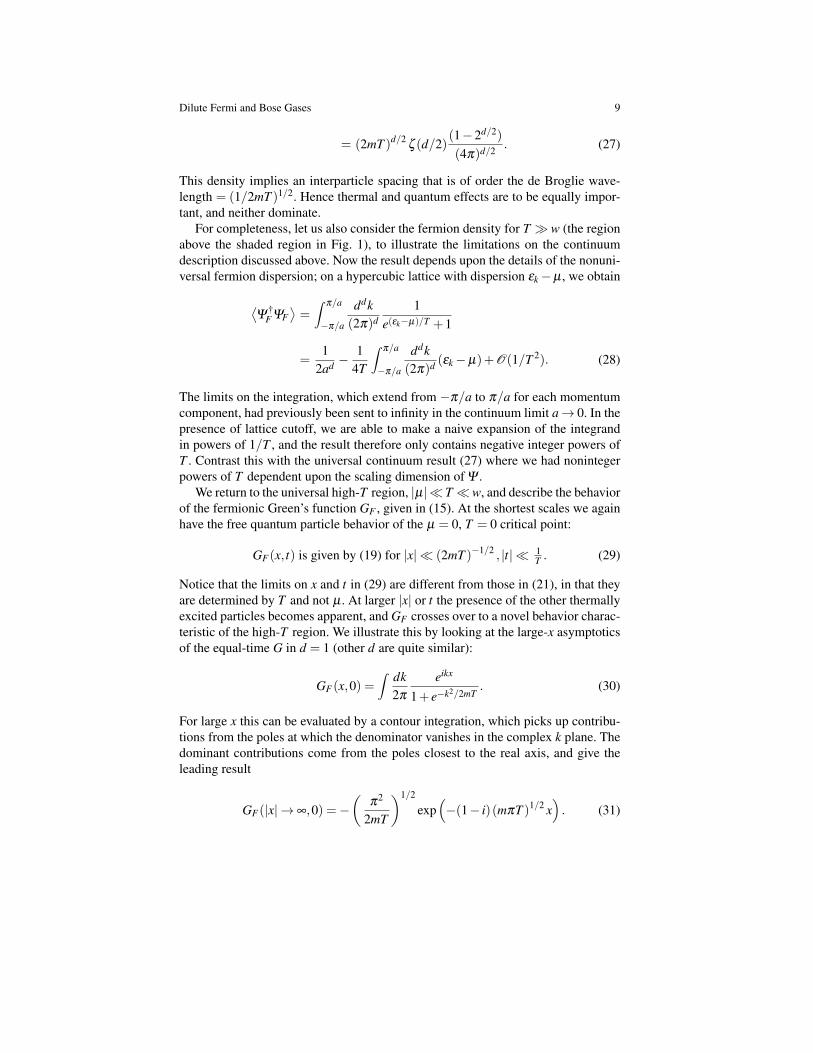
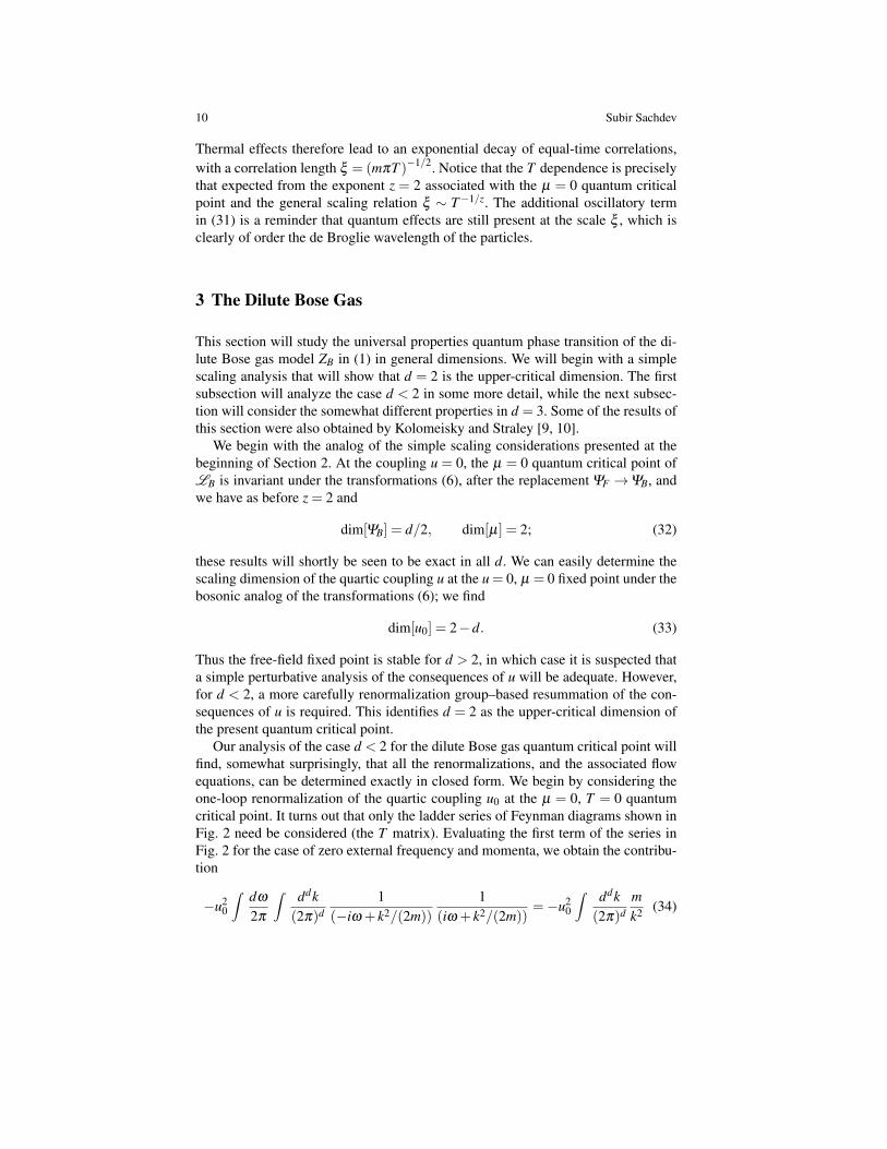
Our analysis of the case d < 2 for the dilute Bose gas quantum critical point willfind, somewhat surprisingly, that all the renormalizations, and the associated flowequations, can be determined exactly in closed form. We begin by considering theone-loop renormalization of the quartic coupling u0 at the µ = 0, T = 0 quantumcritical point. It turns out that only the ladder series of Feynman diagrams shown inFig. 2 need be considered (the T matrix). Evaluating the first term of the series inFig. 2 for the case of zero external frequency and momenta, we obtain the contribu-tion

−u20

∫ dω

2π

∫ ddk(2π)d

1(−iω + k2/(2m))

1(iω + k2/(2m))

=−u20

∫ ddk(2π)d

mk2 (34)

Dilute Fermi and Bose Gases 11

+

+ + ...

Fig. 2 The ladder series of diagrams that contribute the renormalization of the coupling u in ZBfor d < 2.

(the remaining ladder diagrams are powers of (34) and form a simple geometricseries). Notice the infrared singularity for d < 2, which is cured by moving awayfrom the quantum critical point, or by external momenta.

We can proceed further by a simple application of the momentum shell RG. Notethat we will apply cutoff Λ only in momentum space. The RG then proceeds byintegrating all frequencies, and momentum modes in the shell between Λe−` andΛ . The renormalization of the coupling u0 is then given by the first diagram inFig. 2, and after absorbing some phase space factors by a redefinition of interactioncoupling

u0 =Λ d−2

2mSdu, (35)

we obtain [6, 7]dud`

= εu− u2

2. (36)

Here Sd = 2/(Γ (d/2)(4π)d/2) is the usual phase space factor, and

ε = 2−d. (37)

Note that for ε > 0, there is a stable fixed point at

u∗ = 2ε, (38)

which will control all the universal properties of ZB.The flow equation (36), and the fixed point value (38) are exact to all orders

in u or ε , and it is not necessary to consider u-dependent renormalizations to thefield scale of ΨB or any of the other couplings in ZB. This result is ultimately aconsequence of a very simple fact: The ground state of ZB at the quantum criticalpoint µ = 0 is simply the empty vacuum with no particles. So any interactions thatappear are entirely due to particles that have been created by the external fields. Inparticular, if we introduce the bosonic Green’s function (the analog of (15))

GB(x, t) =⟨ΨB(x, t)Ψ

†B (0,0)

⟩, (39)

12 Subir Sachdev

then for µ ≤ 0 and T = 0, its Fourier transform G(k,ω) is given exactly by the freefield expression

GB(k,ω) =1

−ω + k2/(2m)−µ. (40)

The field Ψ†

B creates a particle that travels freely until its annihilation at (x, t) by thefield ΨB; there are no other particles present at T = 0, µ ≤ 0, and so the propagatoris just the free field one. The simple result (40) implies that the scaling dimensionsin (32) are exact. Turning to the renormalization of u, it is clear from the diagramin Fig. 2 that we are considering the interactions of just two particles. For these,the only nonzero diagrams are the one shown in Fig. 2, which involve repeatedscattering of just these particles. Formally, it is possible to write down many otherdiagrams that could contribute to the renormalization of u; however, all of thesevanish upon performing the integral over internal frequencies for there is always oneintegral that can be closed in one half of the frequency plane where the integrandhas no poles. This absence of poles is of course just a more mathematical way ofstating that there are no other particles around.

We will consider application of these renormalization group results separatelyfor the cases below and above the upper-critical dimension of d = 2.

3.1 d < 2

First, let us note some important general implications of the theory controlled bythe fixed point interaction (38). As we have already noted, the scaling dimensionsof ΨB and µ are given precisely by their free field values in (32), and the dynamicexponent z also retains the tree-level value z = 2. All these scaling dimensions areidentical to those obtained for the case of the spinless Fermi gas in Section 2. Fur-ther, the presence of a nonzero and universal interaction strength u∗R in (38) impliesthat the bosonic system is stable for the case µ > 0 because the repulsive interac-tions will prevent the condensation of infinite density of bosons (no such interactionwas necessary for the fermion case, as the Pauli exclusion was already sufficient tostabilize the system). These two facts imply that the formal scaling structure of thebosonic fixed point being considered here is identical to that of the fermionic oneconsidered in Section 2 and that the scaling forms of the two theories are identical.In particular, GB will obey a scaling form identical to that for GF in (14) (with a cor-responding scaling function ΦGB ), while the free energy, and associated derivatives,obey (16) (with a scaling function ΦFB ). The universal functions ΦGB and ΦFB canbe determined order by order in the present ε = 2− d expansion, and this will beillustrated shortly.

Although the fermionic and bosonic fixed points share the same scaling dimen-sions, they are distinct fixed points for general d < 2. However, these two fixedpoints are identical precisely in d = 1 [19]. Evidence for this was presented inRef. [5], where the anomalous dimension of the composite operator Ψ 2

B was com-

Dilute Fermi and Bose Gases 13

puted exactly in the ε expansion and was found to be identical to that of the cor-responding fermionic operator. Assuming the identity of the fixed points, we canthen make a stronger statement about the universal scaling function: those for thefree energy (and all its derivatives) are identical ΦFB = ΦFF in d = 1. In particular,from (17) and (18) we conclude that the boson density is given by

〈Q〉=⟨Ψ

†BΨB

⟩=∫ dk

2π

1e(k2/(2m)−µ)/T +1

(41)

in d = 1 only. The operators ΨB and ΨF are still distinct and so there is no reason forthe scaling functions of their correlators to be the same. However, in d = 1, we canrelate the universal scaling function of ΨB to those of ΨF via a continuum version ofthe Jordan-Wigner transformation

ΨB(x, t) = exp(

iπ∫ x

−∞

dyΨ †F (y, t)ΨF(y, t)

)ΨF(x, t). (42)

This identity is applied to numerous exact results in Ref. [17]As not all observables can be computed exactly in d = 1 by the mapping to the

free fermions, we will now consider the ε = 2− d expansion. We will present asimple ε expansion calculation [18] for illustrative purposes. We focus on densityof bosons at T = 0. Knowing that the free energy obeys the analog of (16), we canconclude that a relationship like (5) holds:

⟨Ψ

†BΨB

⟩=

Cd(2mµ)d/2, µ > 0,

0, µ < 0,(43)

at T = 0, with Cd a universal number. The identity of the bosonic and fermionictheories in d = 1 implies from (5) or from (41) that C1 = S1/1 = 1/π . We will showhow to compute Cd in the ε expansion; similar techniques can be used for almostany observable.

Even though the position of the fixed point is known exactly in (38), not allobservables can be computed exactly because they have contributions to arbitraryorder in u. However, universal results can be obtained order-by-order in u, whichthen become a power series in ε = 2− d. As an example, let us examine the loworder contributions to the boson density. To compute the boson density for µ > 0,we anticipate that there is condensate of the boson field ΨB, and so we write

ΨB(x,τ) =Ψ0 +Ψ1(x, t), (44)

where Ψ1 has no zero wavevector and frequency component. Inserting this into LBin (1), and expanding to second order in Ψ1, we get

L1 = −µ|Ψ0|2 +u0

2|Ψ0|4−Ψ

∗1

∂Ψ1

∂τ+

12m|∇Ψ1|2

−µ|Ψ1|2 +u0

2(4|Ψ0|2|Ψ1|2 +Ψ

20 Ψ∗2

1 +Ψ∗2

0 Ψ2

1). (45)

14 Subir Sachdev

This is a simple quadratic theory in the canonical Bose field Ψ1, and its spectrum andground state energy can be determined by the familiar Bogoliubov transformation.Carrying out this step, we obtain the following formal expression for the free energydensity F as a function of the condensate Ψ0 at T = 0:

F (Ψ0) = −µ|Ψ0|2 +u0

2|Ψ0|4 +

12

∫ ddk(2π)d

[(k2

2m−µ +2u0|Ψ0|2

)2

− u20|Ψ0|4

1/2

−(

k2

2m−µ +2u0|Ψ0|2

)]. (46)

To obtain the physical free energy density, we have to minimize F with respectto variations in Ψ0 and to substitute the result back into (46). Finally, we can takethe derivative of the resulting expression with respect to µ and obtain the requiredexpression for the boson density, correct to the first two orders in u0:

⟨Ψ

†BΨB

⟩=

µ

u0+

12

∫ ddk(2π)d

[1− k2√

k2(k2 +4mµ)

]. (47)

To convert (47) into a universal result, we need to evaluate it at the couplingappropriate to the fixed point (38). This is most easily done by the field-theoreticRG. So let us translate the RG equation (36) into this language. We introduce amomentum scale µ (the tilde is to prevent confusion with the chemical potential)and express u0 in terms of a dimensionless coupling uR by

u0 = uR(2m)µε

Sd

(1+

uR

2ε

). (48)

The motivation behind the choice of the renormalization factor in (48) is that therenormalized four-point coupling, when expressed in terms of uR, and evaluatedin d = 2− ε , is free of poles in ε as can easily be explicitly checked using (34)and the associated geometric series. Then, we evaluate (47) at the fixed point valueof uR, compute any physical observable as a formal diagrammatic expansion in u0,substitute u0 in favor of uR using (48), and expand the resulting expression in powersof ε . All poles in ε should cancel, but the resulting expression will depend upon thearbitrary momentum scale µ . At the fixed point value u∗R, dependence upon µ thendisappears and a universal answer remains. In this manner we obtain from (47) auniversal expression in the form (43) with

Cd = Sd

[1

2ε+

ln2−14

+O(ε)

]. (49)

Dilute Fermi and Bose Gases 15

T

0

C

0

Superfluid

µ

A

B

DiluteClassical Gas

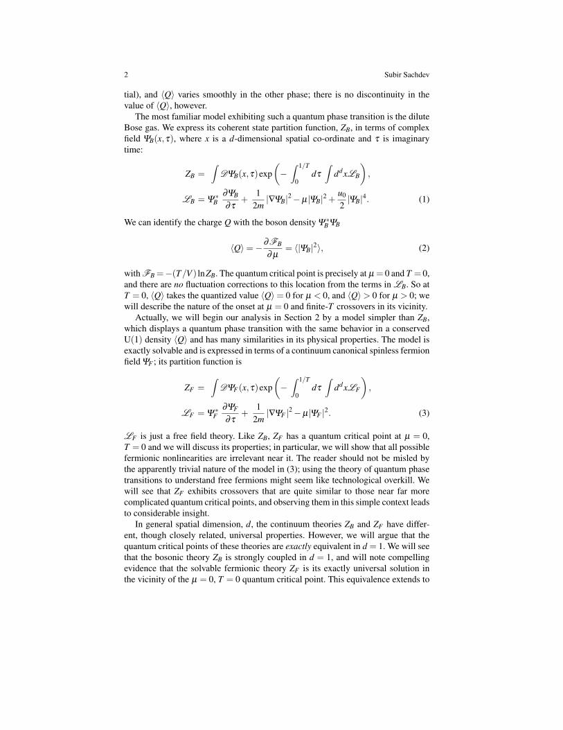
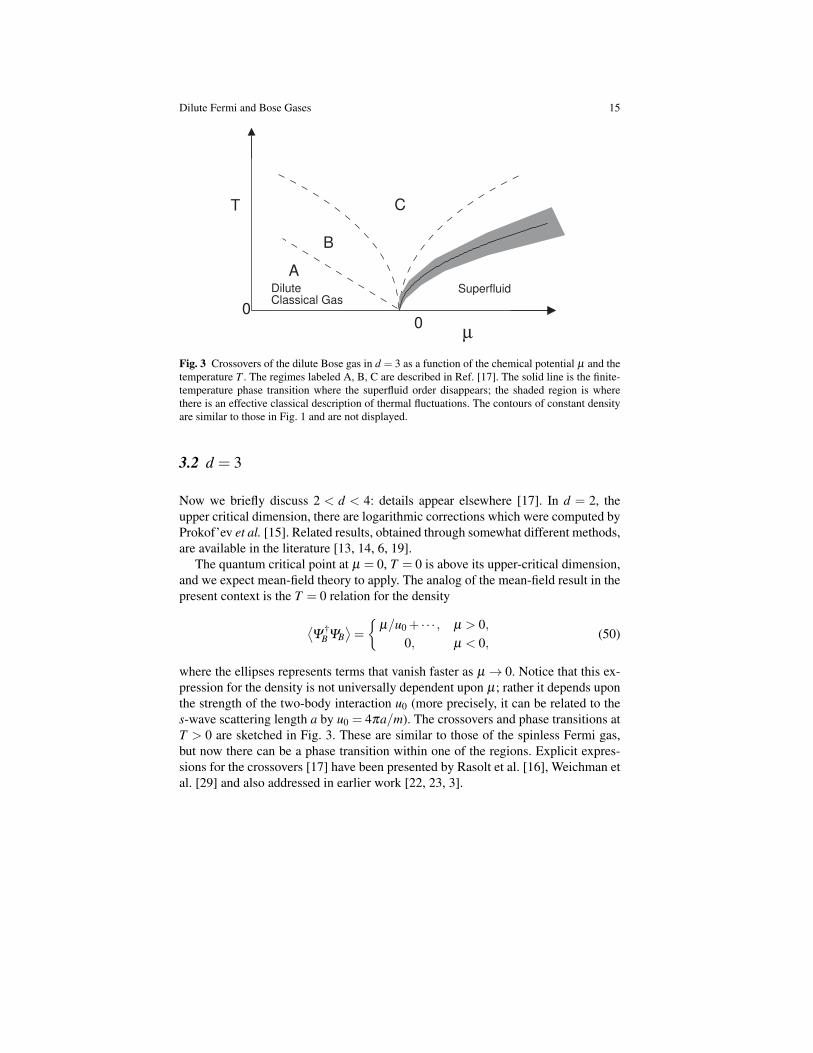
Fig. 3 Crossovers of the dilute Bose gas in d = 3 as a function of the chemical potential µ and thetemperature T . The regimes labeled A, B, C are described in Ref. [17]. The solid line is the finite-temperature phase transition where the superfluid order disappears; the shaded region is wherethere is an effective classical description of thermal fluctuations. The contours of constant densityare similar to those in Fig. 1 and are not displayed.

3.2 d = 3

Now we briefly discuss 2 < d < 4: details appear elsewhere [17]. In d = 2, theupper critical dimension, there are logarithmic corrections which were computed byProkof’ev et al. [15]. Related results, obtained through somewhat different methods,are available in the literature [13, 14, 6, 19].

The quantum critical point at µ = 0, T = 0 is above its upper-critical dimension,and we expect mean-field theory to apply. The analog of the mean-field result in thepresent context is the T = 0 relation for the density

⟨Ψ

†BΨB

⟩=

µ/u0 + · · · , µ > 0,

0, µ < 0,(50)

where the ellipses represents terms that vanish faster as µ → 0. Notice that this ex-pression for the density is not universally dependent upon µ; rather it depends uponthe strength of the two-body interaction u0 (more precisely, it can be related to thes-wave scattering length a by u0 = 4πa/m). The crossovers and phase transitions atT > 0 are sketched in Fig. 3. These are similar to those of the spinless Fermi gas,but now there can be a phase transition within one of the regions. Explicit expres-sions for the crossovers [17] have been presented by Rasolt et al. [16], Weichman etal. [29] and also addressed in earlier work [22, 23, 3].

16 Subir Sachdev

4 The Dilute Spinful Fermi Gas: the Feshbach Resonance

This section turns to the case of the spinful Fermi gas with short-range interactions;as we noted in the introduction, this is a problem which has acquired renewed im-portance because of the new experiments on ultracold fermionic atoms.

The partition function of the theory examined in this section was displayed in(4). The renormalization group properties of this theory in the zero density limit areidentical to those the dilute Bose gas considered in Section 3. The scaling dimen-sions of the couplings are the same, the scaling dimension of ΨFσ is d/2 as for ΨBin (32), and the flow of the u is given by (36). Thus for d < 2, a spinful Fermi gaswith repulsive interactions is described by the stable fixed point in (38).

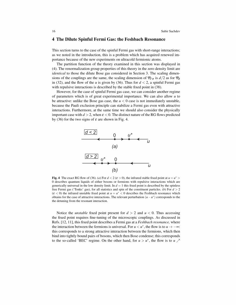
However, for the case of spinful Fermi gas case, we can consider another regimeof parameters which is of great experimental importance. We can also allow u tobe attractive: unlike the Bose gas case, the u < 0 case is not immediately unstable,because the Pauli exclusion principle can stabilize a Fermi gas even with attractiveinteractions. Furthermore, at the same time we should also consider the physicallyimportant case with d > 2, when ε < 0. The distinct nature of the RG flows predictedby (36) for the two signs of ε are shown in Fig. 4.

0 u*

u

d < 2

0u*

u

d > 2

(a)

(b)

Fig. 4 The exact RG flow of (36). (a) For d < 2 (ε > 0), the infrared stable fixed point at u = u∗ >0 describes quantum liquids of either bosons or fermions with repulsive interactions which aregenerically universal in the low density limit. In d = 1 this fixed point is described by the spinlessfree Fermi gas (‘Tonks’ gas), for all statistics and spin of the constituent particles. (b) For d > 2(ε < 0) the infrared unstable fixed point at u = u∗ < 0 describes the Feshbach resonance whichobtains for the case of attractive interactions. The relevant perturbation (u−u∗) corresponds to thethe detuning from the resonant interaction.

Notice the unstable fixed point present for d > 2 and u < 0. Thus accessingthe fixed point requires fine-tuning of the microscopic couplings. As discussed inRefs. [12, 11], this fixed point describes a Fermi gas at a Feshbach resonance, wherethe interaction between the fermions is universal. For u < u∗, the flow is to u→−∞:this corresponds to a strong attractive interaction between the fermions, which thenbind into tightly bound pairs of bosons, which then Bose condense; this correspondsto the so-called ‘BEC’ regime. On the other hand, for u > u∗, the flow is to u

Dilute Fermi and Bose Gases 17

0, and the weakly interacting fermions then form the Bardeen-Cooper-Schrieffer(BCS) superconducting state.

Note that the fixed point at u= u∗ for ZFs has two relevant directions for d > 2. Asin the other problems considered earlier, one corresponds to the chemical potentialµ . The other corresponds to the deviation from the critical point u− u∗, and this(from (36)) has RG eigenvalue −ε = d− 2 > 0. This perturbation corresponds tothe “detuning” from the Feshbach resonance, ν (not to be confused with the symbolfor the correlation length exponent); we have ν ∝ u−u∗. Thus we have

dim[µ] = 2 , dim[ν ] = d−2. (51)

These two relevant perturbations will have important consequences for the phasediagram, as we will see shortly.

For now, let us understand the physics of the Feshbach resonance better. Forthis, it is useful to compute the two body T matrix exactly by summing the graphsin Fig. 2, along with a direct interaction first order in u0. The second order termwas already evaluated for the bosonic case in (34) for zero external momentum andfrequency, and has an identical value for the present fermionic case. Here, however,we want the off-shell T -matrix, for the case in which the incoming particles havemomenta k1,2, and frequencies ω1,2. Actual for the simple momentum-independentinteraction u0, the T matrix depends only upon the sums k = k1 + k2 and ω = ω1 +ω2, and is independent of the final state of the particles, and the diagrams in Fig. 2form a geometric series. In this manner we obtain

1T (k, iω)

=1u0

+∫ dΩ

2π

∫ dd p(2π)d

1(−i(Ω +ω)+(p+ k)2/(2m))

1(iΩ + p2/(2m))

=1u0

+∫

Λ

0

dd p(2π)d

mp2 +

Γ (1−d/2)(4π)d/2 md/2

[−iω +

k2

4m

]d/2−1

. (52)

In d = 3, the s-wave scattering amplitude of the two particles, f0, is related tothe T -matrix at zero center of mass momentum and frequency k2/m by f0(k) =−mT (0,k2/m)/(4π), and so we obtain

f0(k) =1

−1/a− ik(53)

where the scattering length, a, is given by

1a=

4π

mu0+∫

Λ

0

d3 p(2π)3

4π

p2 . (54)

For u0 < 0, we see from (54) that there is a critical value of u0 where the scatteringlength diverges and changes sign: this is the Feshbach resonance. We identify thiscritical value with the fixed point u = u∗ of the RG flow (36). It is conventional to

18 Subir Sachdev

identify the deviation from the Feshbach resonance by the detuning ν

ν ≡−1a. (55)

Note that ν ∝ u− u∗, as claimed earlier. For ν > 0, we have weak attractive inter-actions, and the scattering length is negative. For ν < 0, we have strong attractiveinteractions, and a positive scattering length. Importantly, for ν < 0, there is a two-particle bound state, whose energy can be deduced from the pole of the scatteringamplitude; recalling that the reduced mass in the center of mass frame is m/2, weobtain the bound state energy, Eb

Eb =−ν2

m. (56)

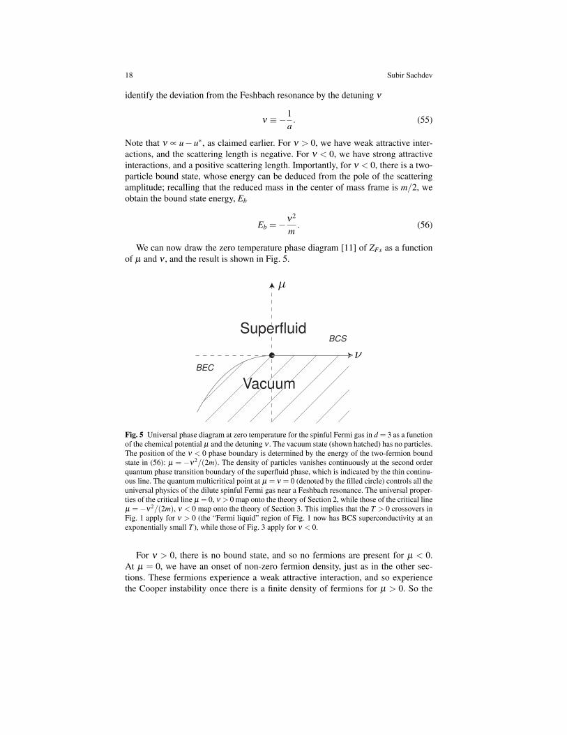
We can now draw the zero temperature phase diagram [11] of ZFs as a functionof µ and ν , and the result is shown in Fig. 5.

Superfluid

Vacuum

BCS

BEC

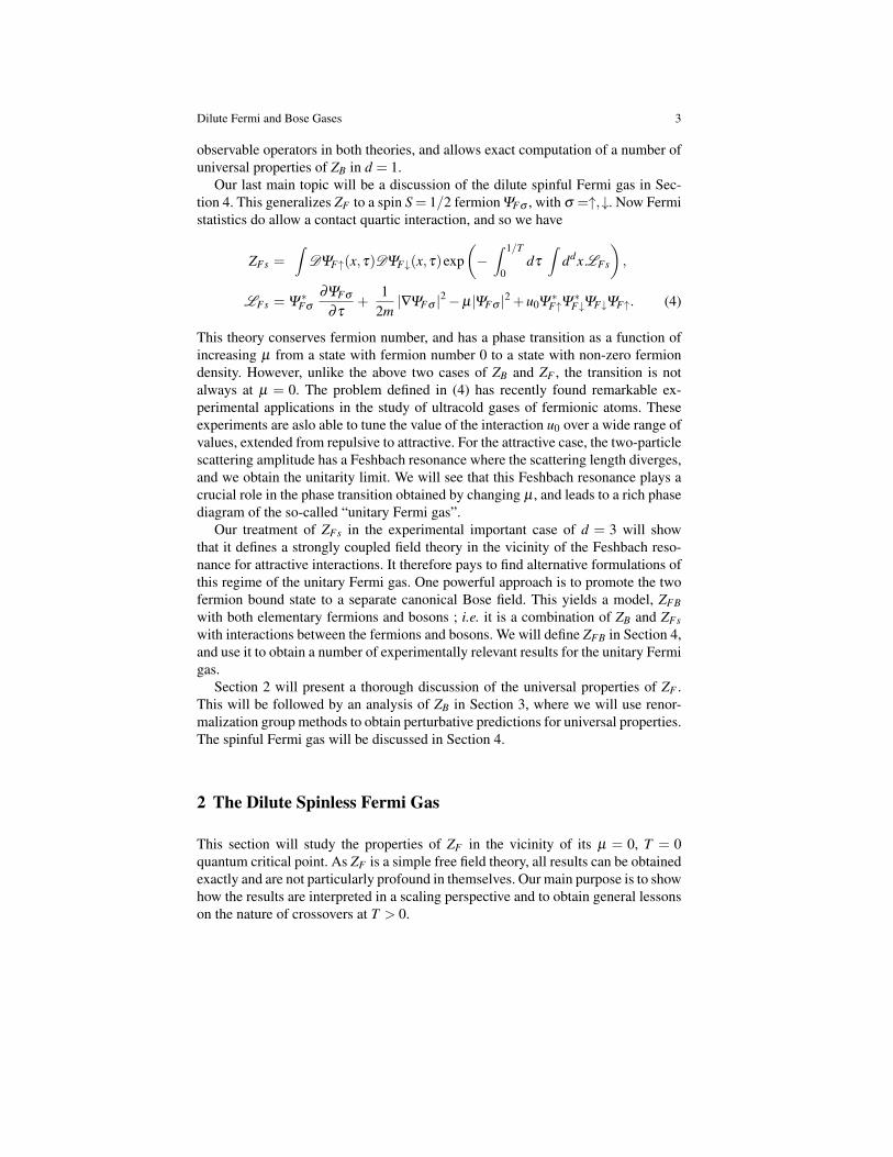
Fig. 5 Universal phase diagram at zero temperature for the spinful Fermi gas in d = 3 as a functionof the chemical potential µ and the detuning ν . The vacuum state (shown hatched) has no particles.The position of the ν < 0 phase boundary is determined by the energy of the two-fermion boundstate in (56): µ = −ν2/(2m). The density of particles vanishes continuously at the second orderquantum phase transition boundary of the superfluid phase, which is indicated by the thin continu-ous line. The quantum multicritical point at µ = ν = 0 (denoted by the filled circle) controls all theuniversal physics of the dilute spinful Fermi gas near a Feshbach resonance. The universal proper-ties of the critical line µ = 0, ν > 0 map onto the theory of Section 2, while those of the critical lineµ =−ν2/(2m), ν < 0 map onto the theory of Section 3. This implies that the T > 0 crossovers inFig. 1 apply for ν > 0 (the “Fermi liquid” region of Fig. 1 now has BCS superconductivity at anexponentially small T ), while those of Fig. 3 apply for ν < 0.

For ν > 0, there is no bound state, and so no fermions are present for µ < 0.At µ = 0, we have an onset of non-zero fermion density, just as in the other sec-tions. These fermions experience a weak attractive interaction, and so experiencethe Cooper instability once there is a finite density of fermions for µ > 0. So the

Dilute Fermi and Bose Gases 19

ground state for µ > 0 is a paired Bardeen-Cooper-Schrieffer (BCS) superfluid, asindicated in Fig. 5. For small negative scattering lengths, the BCS state modifiesthe fermion state only near the Fermi level. Consequently as µ 0 (specificallyfor µ < ν2/m), we can neglect the pairing in computing the fermion density. Wetherefore conclude that the universal critical properties of the line µ = 0, ν > 0 mapprecisely on to two copies (for the spin degeneracy) of the non-interacting fermionmodel ZF studied in Section 2. In particular the T > 0 properties for ν > 0 will maponto the crossovers in Fig. 1. The only change is that the BCS pairing instabilitywill appear below an exponentially small T in the “Fermi liquid” regime. However,the scaling functions for the density as a function of µ/T will remain unchanged.

For ν < 0, the situation changes dramatically. Because of the presence of thebound state (56), it will pay to introduce fermions even for µ < 0. The chemicalpotential for a fermion pair is 2µ , and so the threshold for having a non-zero densityof paired fermions is µ = Eb/2. This leads to the phase boundary shown in Fig. 5at µ = −ν2/(2m). Just above the phase boundary, the density of fermion pairs insmall, and so these can be treated as canonical bosons. Computations of the inter-actions between these bosons [11] show that they are repulsive. Therefore we maptheir dynamics onto those of the dilute Bose gas studied in Section 3. Thus the uni-versal properties of the critical line µ = −ν2/(2m) are equivalent to those of ZB.Specifically, this means that the T > 0 properties across this critical line map ontothose of Fig. 3.

Thus we reach the interesting conclusion that the Feshbach resonance at µ = ν =0 is a multicritical point separating the density onset transitions of ZF (Section 2)and ZB (Section 3). This conclusion can be used to sketch the T > 0 extension ofFig. 5, on either side of the ν = 0 line.

We now need a practical method of computing universal properties of ZFs nearthe µ = ν = 0 fixed point, including its crossovers into the regimes described by ZFand ZB. The fixed point (36) of ZFs provides an expansion of the critical theory inthe powers of ε = 2− d. However, observe from Fig. 4, the flow for u < u∗ is tou→−∞. The latter flow describes the crossover into the dilute Bose gas theory, ZB,and so this cannot be controlled by the 2−d expansion. The following subsectionswill propose two alternative analyses of the Feshbach resonant fixed point whichwill address this difficulty.

4.1 The Fermi-Bose Model

One successful approach is to promote the two fermion bound state in (56) to acanonical boson field ΨB. This boson should also be able to mix with the scatteringstates of two fermions. We are therefore led to consider the following model

ZFB =∫

DΨF↑(x,τ)DΨF↓(x,τ)DΨB(x,τ)exp(−∫

dτddxLFB

),

20 Subir Sachdev

LFB = Ψ∗

Fσ

∂ΨFσ

∂τ+

12m|∇ΨFσ |2−µ|ΨFσ |2

+ Ψ∗

B∂ΨB

∂τ+

14m|∇ΨFσ |2 +(δ −2µ)|ΨB|2

− λ0(Ψ∗

BΨF↑ΨF↓+ΨBΨ∗

F↓Ψ∗

F↑). (57)

Here we have taken the bosons to have mass 2m, because that is the expected massof the two-fermion bound state by Galilean invariance. We have omitted numerouspossible quartic terms between the bosons and fermions above, and these will turnout to be irrelevant in the analysis below.

The conserved U(1) charge for ZFB is

Q =Ψ∗

F↑ΨF↑+Ψ∗

F↓ΨF↓+2Ψ∗

BΨB, (58)

and so ZFB is in the class of models being studied here. The factor of 2 in (58)accounts for the 2µ chemical potential for the bosons in (57). For µ sufficientlynegative it is clear that ZFB will have neither fermions nor bosons present, and so〈Q〉 = 0. Conversely for positive µ , we expect 〈Q〉 6= 0, indicating a transition as afunction of increasing µ . Furthermore, for δ large and positive, the Q density willbe primarily fermions, while for δ negative the Q density will be mainly bosons;thus we expect a Feshbach resonance at intermediate values of δ , which then playsthe role of detuning parameter.

We have thus argued that the phase diagram of ZFB as a function of µ and δ isqualitatively similar to that in Fig. 5, with a Feshbach resonant multicritical pointnear the center. The main claim of this section is that the universal properties of ZFBand ZFs are identical near this multicritical point [11, 12]. Thus, in a strong sense,the theories ZFB and ZFs are equivalent. Unlike the equivalence between ZB and ZF ,which held only in d = 1, the present equivalence applies for d > 2.

We will establish the equivalence by an exact RG analysis of the zero densitycritical theory. We scale the spacetime co-ordinates and the fermion field as in (6),but allow an anomalous dimension ηb for the boson field relative to (32):

x′ = xe−`,

τ′ = τe−z`,

Ψ′

Fσ = ΨFσ ed`/2,

Ψ′

B = ΨBe(d+ηb)`/2

λ′0 = λ0e(4−d−ηb)`/2 (59)

where, as before, we have z = 2. At tree level, the theory ZFB with µ = δ = 0 isinvariant under the transformations in (59) with ηb = 0. At this level, we see thatthe coupling λ0 is relevant for d < 4, and so we will have to consider the influenceof λ0. This also suggests that we may be able to obtain a controlled expansion inpowers of (4−d).

Dilute Fermi and Bose Gases 21

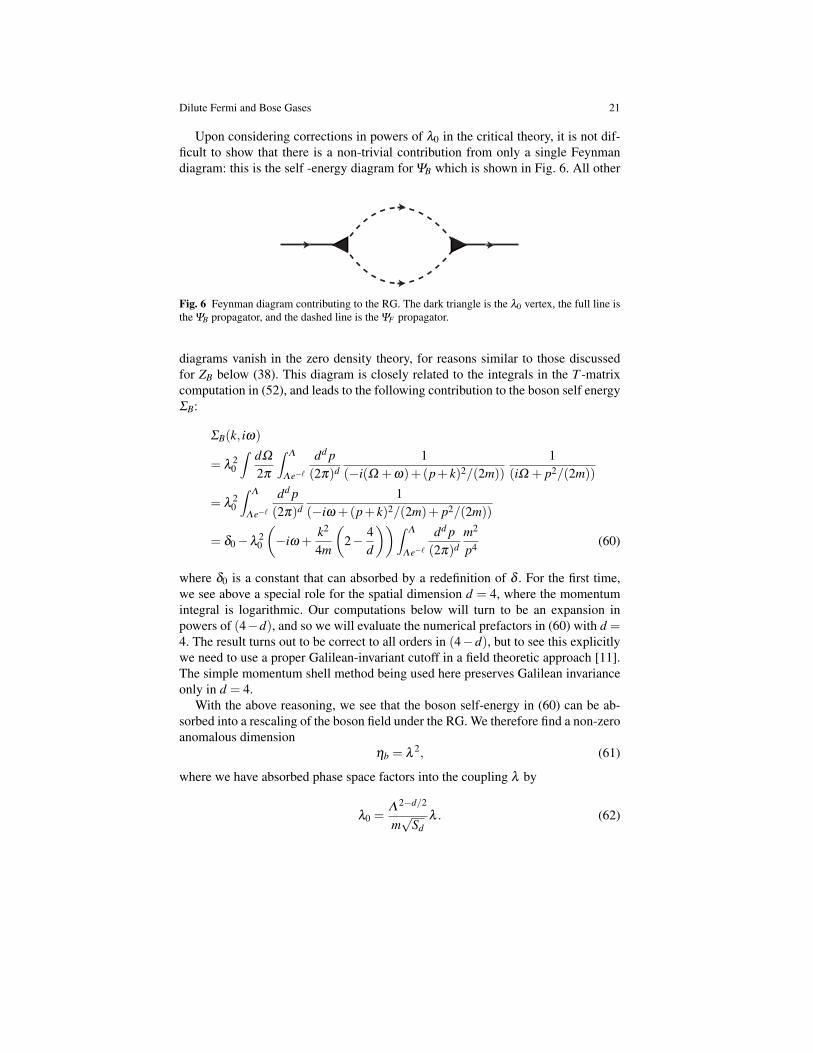
Upon considering corrections in powers of λ0 in the critical theory, it is not dif-ficult to show that there is a non-trivial contribution from only a single Feynmandiagram: this is the self -energy diagram for ΨB which is shown in Fig. 6. All other

Fig. 6 Feynman diagram contributing to the RG. The dark triangle is the λ0 vertex, the full line isthe ΨB propagator, and the dashed line is the ΨF propagator.

diagrams vanish in the zero density theory, for reasons similar to those discussedfor ZB below (38). This diagram is closely related to the integrals in the T -matrixcomputation in (52), and leads to the following contribution to the boson self energyΣB:

ΣB(k, iω)

= λ20

∫ dΩ

2π

∫Λ

Λe−`

dd p(2π)d

1(−i(Ω +ω)+(p+ k)2/(2m))

1(iΩ + p2/(2m))

= λ20

∫Λ

Λe−`

dd p(2π)d

1(−iω +(p+ k)2/(2m)+ p2/(2m))

= δ0−λ20

(−iω +

k2

4m

(2− 4

d

))∫Λ

Λe−`

dd p(2π)d

m2

p4 (60)

where δ0 is a constant that can absorbed by a redefinition of δ . For the first time,we see above a special role for the spatial dimension d = 4, where the momentumintegral is logarithmic. Our computations below will turn to be an expansion inpowers of (4−d), and so we will evaluate the numerical prefactors in (60) with d =4. The result turns out to be correct to all orders in (4−d), but to see this explicitlywe need to use a proper Galilean-invariant cutoff in a field theoretic approach [11].The simple momentum shell method being used here preserves Galilean invarianceonly in d = 4.

With the above reasoning, we see that the boson self-energy in (60) can be ab-sorbed into a rescaling of the boson field under the RG. We therefore find a non-zeroanomalous dimension

ηb = λ2, (61)

where we have absorbed phase space factors into the coupling λ by

λ0 =Λ 2−d/2

m√

Sdλ . (62)

22 Subir Sachdev

With this anomalous dimension, we use (59) to obtain the exact RG equation forλ :

dλ

d`=

(4−d)2

λ − λ 3

2. (63)

For d < 4, this flow has a stable fixed point at λ = λ ∗ =√(4−d). The central claim

of this subsection is that the theory ZFB at this fixed point is identical to the theoryZFs at the fixed point u = u∗ for 2 < d < 4.

Before we establish this claim, note that at the fixed point, we obtain the exactresult for the anomalous dimension of the the boson field

ηb = 4−d. (64)

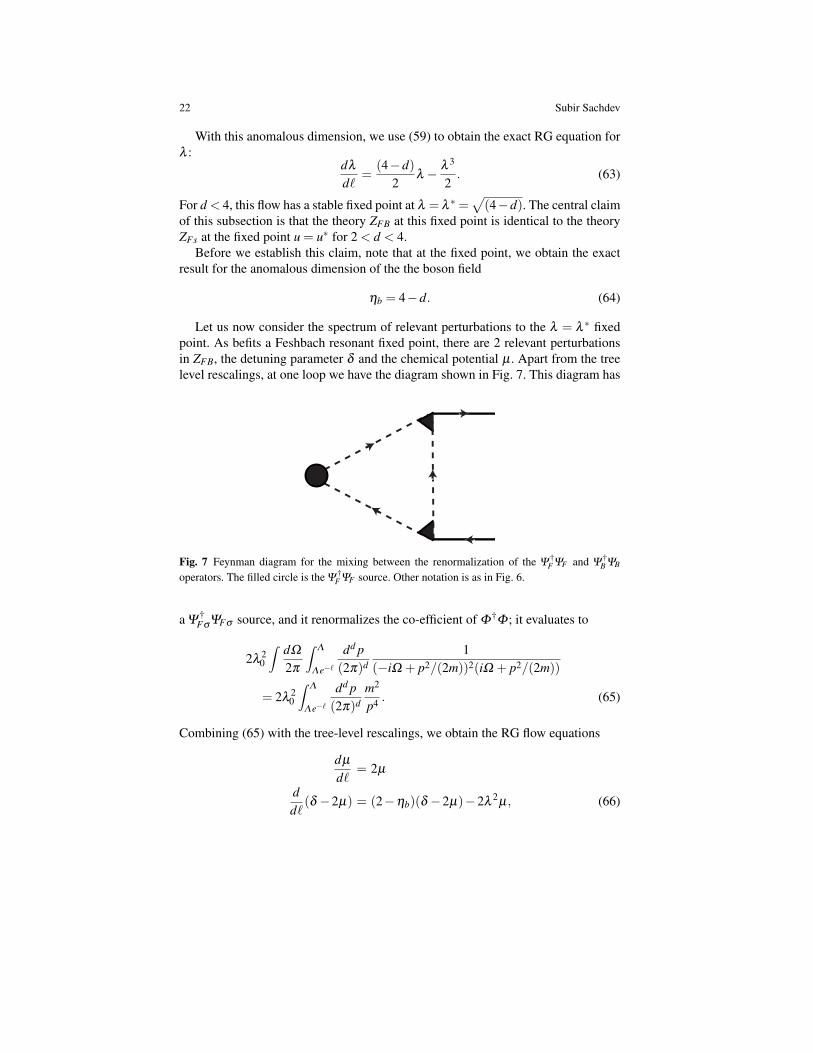
Let us now consider the spectrum of relevant perturbations to the λ = λ ∗ fixedpoint. As befits a Feshbach resonant fixed point, there are 2 relevant perturbationsin ZFB, the detuning parameter δ and the chemical potential µ . Apart from the treelevel rescalings, at one loop we have the diagram shown in Fig. 7. This diagram has

Fig. 7 Feynman diagram for the mixing between the renormalization of the Ψ†

F ΨF and Ψ†

B ΨB

operators. The filled circle is the Ψ†

F ΨF source. Other notation is as in Fig. 6.

a Ψ†

FσΨFσ source, and it renormalizes the co-efficient of Φ†Φ ; it evaluates to

2λ20

∫ dΩ

2π

∫Λ

Λe−`

dd p(2π)d

1(−iΩ + p2/(2m))2(iΩ + p2/(2m))

= 2λ20

∫Λ

Λe−`

dd p(2π)d

m2

p4 . (65)

Combining (65) with the tree-level rescalings, we obtain the RG flow equations

dµ

d`= 2µ

dd`

(δ −2µ) = (2−ηb)(δ −2µ)−2λ2µ, (66)

Dilute Fermi and Bose Gases 23

where the last term arises from (65). With the value of ηb in (61), the second equa-tion simplifies to

dδ

d`= (2−λ

2)δ . (67)

Thus we see that µ and δ are actually eigen-perturbations of the fixed point at λ =λ ∗, and their scaling dimensions are

dim[µ] = 2 , dim[δ ] = d−2. (68)

Note that these eigenvalues coincide with those of ZFs in (51), with δ identified asproportional to the detuning ν . This, along with the symmetries of Q conservationand Galilean invariance, establishes the equivalence of the fixed points of ZFB andZFs.

The utility of the present ZFB formulation is that it can provide a description ofuniversal properties of the unitary Fermi gas in d = 3 via an expansion in (4− d).Further details of explicit computations can be found in Ref. [12].

4.2 Large N expansion

We now return to the model ZFs in (4), and examine it in the limit of a large numberof spin components [11, 27]. We also use the structure of the large N perturbationtheory to obtain exact results relating different experimental observable of the uni-tary Fermi gas.

The basic idea of the large N expansion is to endow the fermion with an addi-tional flavor index a = 1 . . .N/2, to the fermion field is ΨFσa, where we continue tohave σ =↑,↓. Then, we write ZFs as

ZFs =∫

DΨFσa(x,τ)exp(−∫ 1/T

0 dτ∫

ddxLFs

),

LFs = Ψ ∗Fσa∂ΨFσa

∂τ+ 1

2m |∇ΨFσa|2−µ|ΨFσa|2

+2u0

NΨ∗

F↑aΨ∗

F↓aΨF↓bΨF↑b.

(69)

where there is implied sum over a,b = 1 . . .N/2. The case of interest has N = 2, butwe will consider the limit of large even N, where the problem becomes tractable.

As written, there is an evident O(N/2) symmetry in ZFs corresponding to rota-tions in flavor space. In addition, there is U(1) symmetry associated with Q conser-vation, and a SU(2) spin rotation symmetry. Actually, the spin and flavor symmetrycombine to make the global symmetry U(1)×Sp(N), but we will not make much useof this interesting observation.

The large N expansion proceeds by decoupling the quartic term in (69) by aHubbard-Stratanovich transformation. For this we introduce a complex bosonic field

24 Subir Sachdev

ΨB(x,τ) and write

ZFs =∫

DΨFσa(x,τ)DΨB(x,τ)exp(−∫ 1/T

0 dτ∫

ddxLFs

),

LFs = Ψ ∗Fσa∂ΨFσa

∂τ+ 1

2m |∇ΨFσa|2−µ|ΨFσa|2

+N

2|u0||ΨB|2−ΨBΨ

∗F↑aΨ

∗F↓a−Ψ

∗BΨF↓aΨF↑a.

(70)

Here, and below, we assume u0 < 0, which is necessary for being near the Feshbachresonance. Note that ΨB couples to the fermions just like the boson field in the Bose-Fermi model in (57), which is the reason for choosing this notation. If we performthe integral over ΨB in (70), we recover (69), as required. For the large N expansion,we have to integrate over ΨFσa first and obtain an effective action for ΨB. Becausethe action in (70) is Gaussian in the ΨFσa, the integration over the fermion fieldinvolves evaluation of a functional determinant, and has the schematic form

ZFs =∫

DΨB(x,τ)exp(−NSeff [ΨB(x,τ)]) , (71)

where Seff is the logarithm of the fermion determinant of a single flavor. The keypoint is that the only N dependence is in the prefactor in (71), and so the theory ofΨB can controlled in powers of 1/N.

We can expand Seff in powers of ΨB: the p’th term has a fermion loop with pexternal ΨB insertions. Details can be found in Refs. [11, 27]. Here, we only notethat the expansion to quadratic order at µ = δ = T = 0, in which case the co-efficientis precisely the inverse of the fermion T -matrix in (52):

Seff [ΨB(x,τ)] =−12

∫ dω

2π

ddk(2π)d

1T (k, iω)

|ΨB(k,ω)|2 + . . . (72)

Given Seff, we then have to find its saddle point with respect to ΨB. At T = 0, wewill find the optimal saddle point at a ΨB 6= 0 in the region of Fig. 5 with a non-zerodensity: this means that the ground state is always a superfluid of fermion pairs. Thetraditional expansion about this saddle point yields the 1/N expansion, and manyexperimental observables have been computed in this manner [11, 27, 28].

We conclude our discussion of the unitary Fermi gas by deriving an exact rela-tionship between the total energy, E, and the momentum distribution function, n(k),of the fermions [25, 26]. We will do this using the structure of the large N expan-sion. However, we will drop the flavor index a below, and quote results directly forthe physical case of N = 2. As usual, we define the momentum distribution functionby

n(k) = 〈Ψ †Fσ

(k, t)ΨFσ (k, t)〉, (73)

with no implied sum over the spin label σ . The Hamiltonian of the system in (69) isthe sum of kinetic and interaction energies: the kinetic energy is clearly an integral

Dilute Fermi and Bose Gases 25

over n(k) and so we can write

E = 2V∫ ddk

(2π)dk2

2mn(k)+u0V 〈Ψ †

F↑Ψ†

F↓ΨF↓ΨF↑〉

= 2V∫ ddk

(2π)dk2

2mn(k)−u0

∂ lnZFs

∂u0. (74)

where V is the system volume, and all the ΨF fields are at the same x and t. Now letus evaluate the u0 derivative using the expression for ZFs in (70); this leads to

EV

= 2∫ ddk

(2π)dk2

2mn(k)+

1u0〈Ψ ∗B (x, t)ΨB(x, t)〉 . (75)

Now using the expression (54) relating u0 to the scattering length a in d = 3, we canwrite this expression as

EV

=m

4πa〈Ψ ∗BΨB〉+2

∫ d3k(2π)3

k2

2m

(n(k)− 〈Ψ

∗BΨB〉m2

k4

)(76)

This is the needed universal expression for the energy, expressed in terms of n(k)and the scattering length, and independent of the short distance structure of theinteractions.

At this point, it is useful to introduce “Tan’s constant” C, defined by [25, 26]

C = limk→∞

k4n(k). (77)

The requirement that the momentum integral in (76) is convergent in the ultravioletimplies that the limit in (77) exists, and further specifies its value

C = m2 〈Ψ ∗BΨB〉 . (78)

We now note that the relationship n(k)→ m2 〈Ψ ∗BΨB〉/k4 at large k is also asexpected from a scaling perspective. We saw in Section 4.1 that the fermion fieldΨF does not acquire any anomalous dimensions, and has scaling dimension d/2.Consequently n(k) has scaling dimension zero. Next, note that the operator Ψ ∗BΨB isconjugate to the detuning from the Feshbach critical point; from (68) the detuninghas scaling dimension d−2, and so Ψ ∗BΨB has scaling dimension d+z−(d−2) = 4.Combining these scaling dimensions, we explain the k−4 dependence of n(k).

It now remains to establish the claimed exact relationship in (78) as a generalproperty of a spinful Fermi gas near unitarity. As a start, we can examine the largek limit of n(k) in the BCS mean field theory of the superfluid phase: the readercan easily verify that the text-book BCS expressions for n(k) do indeed satisfy (78).However, the claim of Refs. [1, 24] is that (78) is exact beyond mean field theory, andalso holds in the non-superfluid states at non-zero temperatures. A general proof wasgiven in Refs. [24], and relied on the operator product expansion (OPE) applied tothe field theory (70). The OPE is a general method for describing the short distance

26 Subir Sachdev

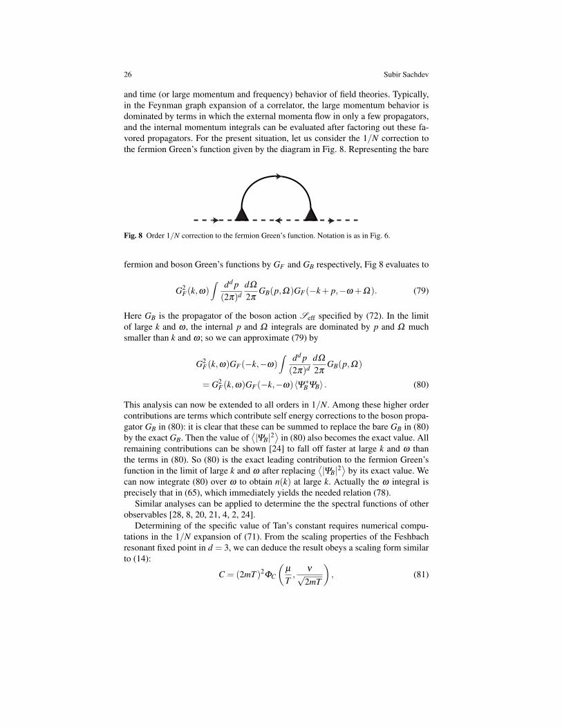
and time (or large momentum and frequency) behavior of field theories. Typically,in the Feynman graph expansion of a correlator, the large momentum behavior isdominated by terms in which the external momenta flow in only a few propagators,and the internal momentum integrals can be evaluated after factoring out these fa-vored propagators. For the present situation, let us consider the 1/N correction tothe fermion Green’s function given by the diagram in Fig. 8. Representing the bare

Fig. 8 Order 1/N correction to the fermion Green’s function. Notation is as in Fig. 6.

fermion and boson Green’s functions by GF and GB respectively, Fig 8 evaluates to

G2F(k,ω)

∫ dd p(2π)d

dΩ

2πGB(p,Ω)GF(−k+ p,−ω +Ω). (79)

Here GB is the propagator of the boson action Seff specified by (72). In the limitof large k and ω , the internal p and Ω integrals are dominated by p and Ω muchsmaller than k and ω; so we can approximate (79) by

G2F(k,ω)GF(−k,−ω)

∫ dd p(2π)d

dΩ

2πGB(p,Ω)

= G2F(k,ω)GF(−k,−ω)〈Ψ ∗BΨB〉 . (80)

This analysis can now be extended to all orders in 1/N. Among these higher ordercontributions are terms which contribute self energy corrections to the boson propa-gator GB in (80): it is clear that these can be summed to replace the bare GB in (80)by the exact GB. Then the value of

⟨|ΨB|2

⟩in (80) also becomes the exact value. All

remaining contributions can be shown [24] to fall off faster at large k and ω thanthe terms in (80). So (80) is the exact leading contribution to the fermion Green’sfunction in the limit of large k and ω after replacing

⟨|ΨB|2

⟩by its exact value. We

can now integrate (80) over ω to obtain n(k) at large k. Actually the ω integral isprecisely that in (65), which immediately yields the needed relation (78).

Similar analyses can be applied to determine the the spectral functions of otherobservables [28, 8, 20, 21, 4, 2, 24].

Determining of the specific value of Tan’s constant requires numerical compu-tations in the 1/N expansion of (71). From the scaling properties of the Feshbachresonant fixed point in d = 3, we can deduce the result obeys a scaling form similarto (14):

C = (2mT )2ΦC

(µ

T,

ν√2mT

), (81)

Dilute Fermi and Bose Gases 27

where ΦC is a dimensionless universal function of its dimensionless arguments; notethat the arguments represent the axes of Fig. 5. The methods of Refs [11, 27] cannow be applied to (78) to obtain numerical results for ΦC in the 1/N expansion. Weillustrate this method here by determining C to leading order in the 1/N expansionat µ = ν = 0. For this, we need to generalize the action (72) for ΨB to T > 0 andgeneral N. Using (52) we can modify (72) to

Seff = NT ∑ωn

∫ d3k8π3 [D0(k,ωn)+D1(k,ωn)] |ΨB(k,ωn)|2, (82)

where D0 is the T = 0 contribution, and D1 is the correction at T > 0:

D0(k,ωn) =m3/2

16π

√−iωn +

k2

4m(83)

D1(k,ωn) =12

∫ d3 p8π3

1(ep2/(2mT )+1)

1(−iω + p2/(2m)+(p+ k)2/(2m))

.

We now have to evaluate 〈Ψ ∗BΨB〉 using the Gaussian action in (82). It is useful todo this by separating the D0 contribution, which allows us to properly deal with thelarge frequency behavior. So we can write

〈Ψ ∗BΨB〉=1N

T ∑ωn

∫ d3k8π3

[1

D0(k,ωn)+D1(k,ωn)− 1

D0(k,ωn)

]+D00. (84)

In evaluating D00 we have to use the usual time-splitting method to ensure that thebosons are normal-ordered, and evaluate the frequency summation by analyticallycontinuing to the real axis:

D00 =1N

∫ d3k8π3 lim

η→0T ∑

ωn

eiωnη

D0(k,ωn)

=16π

Nm3/2

∫ d3k8π3

∫∞

k24m

dΩ

π

1(eΩ/T −1)

1√Ω − k2/(4m)

.

=8.37758

NT 2 (85)

The frequency summation in (84) can be evaluated directly on the imaginary fre-quency axis: the series is convergent at large ωn, and is easily evaluated by a directnumerical summation. Numerical evaulation of (84) now yields

C = (2mT )2(

0.67987N

+O(1/N2)

)(86)

at µ = ν = 0.

28 Subir Sachdev

References

1. Braaten, E., and Platter, L. (2008) Phys. Rev. Lett. 100, 205301.2. Braaten, E., Kang, D., and Platter, L. (2010) arXiv:1001.4518.3. Creswick, R. J., and Wiegel, F. W. (1983) Phys. Rev. A 28, 1579.4. Combescot, R., Alzetto, F., and Leyronas, X. (2009) Phys. Rev. A 79, 0536405. Damle, K., and Sachdev, S. (1996) Phys. Rev. Lett. 76, 4412.6. Fisher, D. S., and Hohenberg, P. C. (1988) Phys. Rev. B 37, 4936.7. Fisher, M. P. A., Weichman, P. B., Grinstein, G., and Fisher, D. S. (1989) Phys. Rev. B 40,

546.8. Haussmann, R., Punk, M., and Zwerger, W. (2009) Phys. Rev. A 80, 063612.9. Kolomeisky, E. B., and Straley, J. P. (1992) Phys. Rev. B 46, 11749.

10. Kolomeisky, E. B., and Straley, J. P. (1992) Phys. Rev. B 46, 13942.11. Nikolic, P., and Sachdev, S. (2007) Phys. Rev. A 75, 033608.12. Nishida, Y., and Son, D. T. (2007) Phys. Rev. A 75, 063617.13. Popov, V. N. (1972) Teor. Mat. Phys. 11, 354.14. Popov, V. N. (1983) Functional Integrals in Quantum Field Theory and Statistical Physics

(D. Reidel, Dordrecht).15. Prokof’ev, N., Ruebenacker, O., and Svistunov, B. (2001) Phys. Rev. Lett. 87, 270402.16. Rasolt, M., Stephen, M. J., Fisher, M. E., and Weichman, P. B. (1984) Phys. Rev. Lett. 53,

798.17. Sachdev, S. Quantum Phase Transitions, Cambridge University Press (1999).18. Sachdev, S., and Senthil, T. (1996) Annals of Physics 251, 76.19. Sachdev, S., Senthil, T., and Shankar, R. (1994) Phys. Rev. B 50, 258.20. Schneider, W., Shenoy, V. B., and Randeria, M. (2009) arXiv:0903.3006.21. Schneider, W., and Randeria, M. (2009) arXiv:0910.2693.22. Singh, K. K. (1975) Phys. Rev. B 12, 2819.23. Singh, K. K. (1978) Phys. Rev. B 17, 324.24. Son, D. T., and Thompson, E. G. (2010) arXiv:1002.0922.25. Tan, S. (2008) Annals of Physics 323, 2952.26. Tan, S. (2008) Annals of Physics 323, 2971.27. Veillette, M. Y., Sheehy, D. E., and Radzihovsky, L. (2007) Phys. Rev. A 75, 043614.28. Veillette, M. Y., Moon, E. G., Lamacraft, A., Radzihovsky, L., Sachdev, S., and Sheehy, D. E.

(2008) Phys. Rev. A 78, 033614.29. Weichman, P. B., Rasolt, M., Fisher, M. E., and Stephen, M. J. (1986) Phys. Rev. B 33, 4632.