Dilemma not Trilemma? Capital Controls and Exchange Rates with Volatile Capital Flows

Emmanuel Farhi Harvard University

Iván Werning

MIT

Paper presented at the 14th Jacques Polak Annual Research Conference Hosted by the International Monetary Fund Washington, DC─November 7–8, 2013 The views expressed in this paper are those of the author(s) only, and the presence

of them, or of links to them, on the IMF website does not imply that the IMF, its Executive Board, or its management endorses or shares the views expressed in the paper.

1144TTHH JJAACCQQUUEESS PPOOLLAAKK AANNNNUUAALL RREESSEEAARRCCHH CCOONNFFEERREENNCCEE NNOOVVEEMMBBEERR 77––88,, 22001133

Dilemma not Trilemma? Capital Controls andExchange Rates with Volatile Capital Flows

Emmanuel FarhiHarvard University

Iván WerningMIT

October 2013

We consider a standard New Keynesian model of a small open economy with nominalrigidities and study optimal capital controls. Consistent with the Mundellian view, wefind that the exchange rate regime is key. However, in contrast with the Mundellianview, we find that capital controls are desirable even when the exchange rate is flexi-ble. Optimal capital controls lean against the wind and help smooth out capital flowdriven business cycles.

1 Introduction

Volatile capital flows have been extensively blamed for episodes of booms and busts inemerging markets (see e.g. Calvo, 1998). What sort of macroeconomic intervention, if any,is required to deal with these episodes?

Mundell’s celebrated trilemma provides a powerful framework to analyze this ques-tion. It emphasizes the importance of the exchange rate regime. With fixed a exchangerate, there is a case for interfering with the free movement of international capital flowsby imposing capital controls in order to regain monetary autonomy (see e.g. Farhi andWerning, 2012; Schmitt-Grohe and Uribe, 2012). By contrast, with a flexible exchange rate,monetary policy is independent and there is no prima facie case for restricting interna-tional capital mobility.

This last conclusion has recently been challenged by policymakers and academics,leading some authors to argue that in contrast to the Mundellian view, there is a dilemma(not a trilemma) in the sense that independent monetary policies are possible only if thecapital account is managed (Rey, 2013). The goal of this paper is to revisit this conclusionusing a model with nominal rigidities in the New Keynesian Small Open Economy tra-dition. Because our model has explicit microfoundations and a formal treatment of gen-

1

eral equilibrium, it is better suited for normative analysis than the traditional Mundell-Flemming models.

We model sudden stops and capital inflow surges as risk premium shocks or wedges,which could also capture time-varying and country-specific borrowing constraints. Ourconclusions have both similarities and differences with the standard Mundellian conclu-sions. Consistent with the Mundellian analysis, we confirm that the exchange rate regimeis key: Optimal capital flows depend importantly on the exchange rate regime. But incontrast to the Mundellian analysis, we find that even with flexible exchange rates, thereis a powerful case for capital controls. More specifically, we find that optimal capital con-trols lean against the wind. To deal with a sudden stop, they take the form of temporarysubsidies on capital inflows / taxes on capital outflows. To deal with a capital inflowsurge, they take the form of temporary taxes on capital inflows / subsidies on capitalinflows.

To understand the effects of capital controls with flexible exchange rates, consider thecase of a sudden stop. Without capital controls but with optimal monetary policy, thesudden stop leads to a sharp depreciation of the nominal exchange rate despite a large in-crease in nominal interest rates, and an abrupt rebalancing of the current account througha drop in consumption. Optimal capital controls take the form of temporary subsidies oncapital inflows / taxes on capital outflows and smooth out these responses: They delivera mitigation of the depreciation of the exchange rate, of the increase in nominal interestrate, of the reversal in the current account, and of the drop in consumption. We traceback the intuition for the optimality of these interventions to the desirability to jointlymanipulate the intertemporal terms of trade and stabilize the macroeconomy using twoimperfect instruments, monetary policy and capital controls.

A large literature in international macroeconomics is motivated by the volatility ofcapital flows, especially “sudden stops”, see Mendoza (2010) and the references therein.Models with financial frictions such as Caballero and Krishnamurthy (2004) emphasizedomestic and international collateral constraints that create inefficiencies and a poten-tial role for intervention in international borrowing, even without nominal rigidities. Arelated strand of work emphasizes pecuniary externalities that work through prices inborrowing constraints, for example Bianchi and Mendoza (2010), Bianchi (2011), Jeanneand Korinek (2010), Korinek (2011). All these papers provide a rationale for “pruden-tial” policies that attempt to prevent excessive borrowing. An important difference withour analysis of capital controls and more generally with the Mundellian logic, is that themodels in these papers are real, and as a result, optimal capital controls are independentof the exchange rate regime.

2

2 A Small Open Economy

We build on Farhi and Werning (2012), which in turn builds on the framework by Galiand Monacelli (2005, 2008). The model is composed of a continuum of open economies.Our main focus is on policy in a single country, which we call Home, taking as giventhe rest of the world, which we call Foreign. However, we also explore the joint policyproblem for the entire world when coordination is possible. In contrast to their simplify-ing assumption of complete markets, we prefer to assume international financial marketsare incomplete. No risk sharing between countries is allowed, only risk free borrowingand lending. Given this assumption, to keep the analysis tractable, we limit our attentionto one-time unanticipated shocks to the economy. Relative to the literature, this is not alimitation since most studies, including Gali-Monacelli, work with linearized equilibriumconditions, so that the response to shocks is unaffected by the presence of future shocks.

2.1 Households

There is a continuum measure one of countries i ∈ [0, 1]. We focus attention on a singlecountry, which we call Home, and can be thought of as a particular value H ∈ [0, 1]. Inevery country, there is a representative household with preferences represented by theutility function

∞

∑t=0

βt

[C1−σ

t1− σ

− N1+φt

1 + φ

], (1)

where Nt is labor, and Ct is a consumption index defined by

Ct =

[(1− α)

1η C

η−1η

H,t + α1η C

η−1η

F,t

] ηη−1

,

where CH,t is an index of consumption of domestic goods given by

CH,t =

(ˆ 1

0CH,t(j)

ε−1ε dj

) εε−1

,

where j ∈ [0, 1] denotes an individual good variety. Similarly, CF,t is a consumption indexof imported goods given by

CF,t =

(ˆ 1

0C

γ−1γ

i,t di

) γγ−1

,

3

where Ci,t is, in turn, an index of the consumption of varieties of goods imported fromcountry i, given by

Ci,t =

(ˆ 1

0Ci,t(j)

ε−1ε dj

) εε−1

.

Thus, ε is the elasticity between varieties produced within a given country, η the elas-ticity between domestic and foreign goods, and γ the elasticity between goods producedin different foreign countries. An important special case obtains when σ = η = γ = 1.We call this the Cole-Obstfeld case, in reference to Cole and Obstfeld (1991). This case ismore tractable and has some special implications that are worth highlighting. Thus, wedevote special attention to it, although we will also derive results away from it.

The parameter α indexes the degree of home bias, and can be interpreted as a measureof openness. Consider both extremes: as α → 0 the share of foreign goods vanishes; asα → 1 the share of home goods vanishes. Since the country is infinitesimal, the lattercaptures a very open economy without home bias; the former a closed economy barelytrading with the outside world.

Households seek to maximize their utility subject to the sequence of budget con-straints

ˆ 1

0PH,t(j)CH,t(j)dj +

ˆ 1

0

ˆ 1

0Pi,t(j)Ci,t(j)djdi + Dt+1 +

ˆ 1

0Ei,tDi

t+1di

≤WtNt + Πt + Tt + (1 + it−1)Dt +

ˆ 1

0

1 + τt−1

1 + τit−1

Ψt−1

Ψi,t−1Ei,t(1 + ii

t−1)Ditdi

for t = 0, 1, 2, . . . In this inequality, PH,t(j) is the price of domestic variety j, Pi,t is theprice of variety j imported from country i, Wt is the nominal wage, Πt represents nom-inal profits and Tt is a nominal lump sum transfer. All these variables are expressed indomestic currency. The portfolio of home agents is composed of home and foreign bondholding: Dt is home bond holdings of home agents, Di

t is bond holdings of country i ofhome agents. The returns on these bonds are determined by the nominal interest ratein the home country it, the nominal interest rate ii

t in country i, and the evolution of thenominal exchange rate Ei,t between home and country i. Capital controls are modeled asfollows: τt is a subsidy on capital outflows (tax on capital inflows) in the home country,and similarly τi

t is a subsidy on capital outflows (tax on capital inflows) in country i. Theproceeds of these taxes are rebated lump sum to the households at Home and country i,respectively.

Importantly, we have introduced risk premium shocks Ψt and Ψi,t as wedges between

4

foreign investors and the home country, in addition to capital controls for all i ∈ [0, 1].We do not attempt to model these wedges endogenously. Although our model lacks un-certainty, it could stand in for the risks of investing in the home country, if these risksare not equally valued between borrowers and lenders. It may also represent investor’spreferences for a particular country’s bonds along the lines of portfolio-balance modelsa la Black (1973) and Kouri (1976). Risk premium shocks can also be thought of captur-ing time-varying and country-specific borrowing constraints—the risk premium shock issimply the multiplier on the borrowing constraint.

Capital controls and risk premium wedges enter the agent’s budget constraint in asimilar way. The key difference between the two is that the domestic subsidy on outflowsis financed with a lump sum tax on domestic agents, while the risk premium wedge isfinanced with a lump sum tax at the world level: the lump sum rebate Tt is given by

Tt = −ˆ 1

0

ˆ 1

0(

Ψi,t−1

Ψj,t−1− 1)

1

1 + τjt

(1 + ijt−1)Ej,tD

j,it didj

−ˆ 1

0

τt−1

1 + τit−1

Ψt−1

Ψi,t−1Ei,t(1 + ii

t−1)Ditdi + τLWtNt,

where Di,jt is bond holdings of country j of agents of country i, and τL is a constant labor

tax. Actually, in most of our analysis, we consider a small open economy. We treat therest of the world as symmetric countries which do not face risk premium shocks Ψi,t = 0and do not impose capital controls τi

t = 0. In that case, the lump sum rebate becomes

Tt = −τt−1Ψt−1E∗t (1 + i∗t−1)D∗t + τLWtNt,

and the difference between risk premium wedges and capital controls appears most clearly.Risk premium shocks affects equally the interest rate at which home agents perceive theycan borrow and lend to the rest of the world, and the interest rate at which the homecountry as a whole can borrow and lend to the rest of the world.By contrast, capital con-trols only affect the interest rate at which home agents perceive they can borrow and lendto the rest of the world, but not the interest rate at which the home country as a wholecan borrow and lend to the rest of the world.1

1This observation already already gives a sense of why the naive idea that capital controls should simplyoffset risk premium shocks τt = Ψ−1

t − 1 is not supported by our analysis.

5

2.2 Firms

Technology. A typical firm in the home economy produces a differentiated good with alinear technology given by

Yt(j) = ANt(j). (2)

Price-setting assumptions. We will consider a variety of price setting assumptions: flex-ible prices, one-period in advance sticky prices, and sticky prices a la Calvo.

As in Gali and Monacelli (2005), we maintain the assumption that the Law of OnePrice (LOP) holds so that at all times, the price of a given variety in different countries isidentical once expressed in the same currency. This assumption is sometimes known asProducer Currency Pricing (PCP).2

First, consider the case of flexible prices. We allow for a constant employment tax 1 +τL, so that real marginal cost deflated by Home PPI is given by MCt =

1+τL

AWtPH,t

.We takethis employment tax to be constant in our model. We explain below how it is determined.Firm j optimally sets its price PH,t(j) to maximize

maxPH,t(j)

(PH,t(j)Yt|t − PH,tMCtYt|t)

where Yt|t =(

PH,t(j)PH,t

)−εYt, taking the sequences for MCt, Yt and PH,t as given. Second,

we consider the case where prices are perfectly rigid. Third we consider the case whereare set one period in advance as in Obstfeld and Rogoff (1995). Since we consider only onetime-unanticipated shocks around the symmetric deterministic steady state, this simplymeans that prices are fixed at t = 0 and flexible for t ≥ 1. Fourth, we consider Calvo pricesetting, where in every period, a randomly selected fraction 1− δ of firms can reset theirprices. Those firms that get to reset their price choose a reset price Pr

t to solve

maxPr

t

∞

∑k=0

δk

(k

∏h=1

11 + it+h

)(Pr

t Yt+k|t − PH,tMCtYt+k|t)

where Yt+k|t =(

Prt

PH,t+k

)−εYt+k.

2This is sometimes contrasted with the assumption of Local Currency Pricing (LCP), where each va-riety’s price is set separately for each country and quoted (and potentially sticky) in that country’s localcurrency. Thus, LOP does not necessarily hold. It has been shown by Devereux and Engel (2003) that LCPand PCP may have different implications for monetary policy.

6

2.3 Terms of Trade, Exchange Rates and UIP

It is useful to define the following price indices: home’s Consumer Price Index (CPI) Pt =

[(1− α)P1−ηH,t + αP1−η

F,t ]1

1−η , home’s Producer Price Index (PPI) PH,t = [´ 1

0 PH,t(j)1−εdj]1

1−ε ,

and the index for imported goods PF,t = [´ 1

0 P1−γi,t di]

11−γ , where Pi,t = [

´ 10 Pi,t(j)1−εdj]

11−ε

is country i’s PPI.Let Ei,t be nominal exchange rate between home and i (an increase in Ei,t is a de-

preciation of the home currency). Because the Law of One Price holds, we can writePi,t(j) = Ei,tPi

i,t(j) where Pii,t(j) is country i’s price of variety j expressed in its own cur-

rency. Similarly, Pi,t = Ei,tPii,t where Pi

i,t = [´ 1

0 Pii,t(j)1−ε]

11−ε is country i’s domestic PPI in

terms of country i’s own currency. We therefore have

PF,t = EtP∗t

where P∗t = [´ 1

0 Pi1−γi,t di]

11−γ is the world price index and Et is the effective nominal ex-

change rate.3

The terms of trade are defined by

St =PF,t

PH,t=

EtP∗tPH,t

.

Similarly let the real exchange rate be

Qt =EtP∗t

Pt.

The risk premium shocks Ψt and Ψi,t introduce a wedge in the UIP condition

1 + it =Ψt

Ψi,t

1 + τt

1 + τit(1 + ii

t)Ei,t+1

Ei,t.

2.4 Equilibrium Conditions with Symmetric Rest of the World

We now summarize the equilibrium conditions. For simplicity of exposition, we focuson the case where all foreign countries are identical. We assume that there are no riskpremium shocks in the foreign countries. Moreover, we assume that foreign countriesdo not impose capital controls. We denote foreign variables with a star. Taking foreignvariables as given, equilibrium in the home country can be described by the following

3The effective nominal exchange rate is defined as Et = [´ 1

0 E1−γi,t Pi1−γ

i,t di]1

1−γ /[´ 1

0 Pi1−γi,t di]

11−γ .

7

equations. We find it convenient to group these equations into two blocks, which werefer to as the demand block and the supply block.

The demand block is independent of the nature of price setting. It is composed of theBackus-Smith condition

Ct = ΘtC∗tQ1σt , (3)

where Θt is a relative Pareto weight whose evolution is given by equation (7) below, bythe equation relating the real exchange rate to the terms of trade

Qt =[(1− α) (St)

η−1 + α] 1

η−1 , (4)

the goods market clearing condition

Yt = (1− α)

(Qt

St

)−η

Ct + αSγt C∗t , (5)

the labor market clearing condition

Nt =Yt

AH,t∆t (6)

where ∆t is an index of price dispersion ∆t =´ 1

0

(PH,t(j)

PH,t

)−ε, the Euler equation

1 + it = β−1 Cσt+1

Cσt

Πt+1

where Πt = Pt+1Pt

= ΠH,tStQt

Qt−1St−1

is CPI inflation, the arbitrage condition between homeand foreign bonds

Θσt+1

Θσt

=1 + it

1 + i∗Et

Et+1, (7)

and the country budget constraint

NFAt = −C∗−σt

(S−1

t Yt −Q−1t Ct

)+ βΨ−1

t NFAt+1 (8)

where NFAt is the country’s net foreign assets at t, which for convenience, we measurein the foreign price at home PF,t as the numeraire, and which we adjust by the foreignmarginal utility of consumption C∗−σ

t . The country budget constraint is derived fromthe consumer’s budget constraint after substituting out the lump-sum transfer. Undergovernment budget balance the transfer equals the sum of the revenue from the labor tax

8

and the tax on foreign investors, net of the revenue lost to subsidize domestic residents’investments abroad.4 We also impose a No-Ponzi condition so that we can write thebudget constraint in present-value form

0 = −∞

∑t=0

βt( t−1

∏s=0

Ψ−1s)C∗−σ

t

(S−1

t Yt −Q−1t Ct

). (9)

The supply block varies with the nature of price setting. With flexible prices, it boilsdown to the following condition, which combines the household and firm’s first-orderconditions,

C−σt S−1

t Qt = M1 + τL

ANφ

t (10)

where M = εε−1 is the desired markup of price over marginal cost, together with the no

price dispersion assumption ∆t = 1. With one period in advance price stickiness, theonly difference is that at t = 0, all prices are fixed. This means that S0 = E0

P∗0PH,0

whereP∗0 and PH,0 are fixed. Finally with Calvo price setting, which will be our main focus, thesupply block is more complex. It is composed of the equations summarizing the first-order condition for optimal price setting.

1− δΠε−1H,t

1− δ=

(Ft

Kt

)ε−1

,

Kt = M1 + τL

AYtN

φt Πε

H,t + δβKt+1,

Ft = YtC−σt S−1

t QtΠε−1H,t + δβFt+1,

together with an equation determining the evolution of price dispersion

∆t = h(∆t−1, ΠH,t),

where h(∆, Π) = δ∆Πε + (1 − δ)(

1−δΠε−1

1−δ

) εε−1 . We will only analyze a log-linearized

version of the model with Calvo price setting.

4We do not require budget balance but since Ricardian equivalence holds here, all other governmentfinancing schemes have the same implications.

9

2.5 Steady State Labor Tax

We allow for a constant tax on labor in each country. We pin this tax rate down by assum-ing that it is optimally set by each country and considering a symmetric steady state withflexible prices.5 We refer the reader to Farhi and Werning (2012) for a derivation of thefollowing result.

Proposition 1 (Steady State Tax). Suppose prices are flexible, that productivity is constantacross time and countries and there are no export demand shocks. Then at a symmetric steadystate, τL = 1

M(1−α)(η−1)+γ

(1−α)(η−1)+γ−α− 1 and optimal capital controls are equal to zero.

From each country’s perspective, the labor tax is the result of a balancing act betweenoffsetting the monopoly distortion of individual producers and exerting some monopolypower as a country. The two terms in the optimal tax formula reflect the two legs of thistradeoff.

2.6 Shocks

We assume that the economy is initially at the deterministic symmetric steady state andcharacterize the optimal use of capital controls for the home country in response to riskpremium shocks. We choose to focus on these shocks because many discussions of capitalcontrols, especially in developing countries, focus on capital inflow surges that are takento be exogenous fluctuations in investor sentiments. It allows to flexibly capture episodesof capital flow surges (negative risk premium shocks) and sudden stops (positive riskpremium shocks).

3 Flexible Prices and Rigid Prices in the Non-Linear Model

In this section, we treat the case of perfectly flexible and perfectly rigid prices in the non-linear model. In Section 4, we treat the intermediate case of sticky but not perfectly rigidprices using the Calvo model of price adjustment. There, we find it more convenient towork with a log-linearized version of the model.

We start the economy at a symmetric steady state. At t = 0, the economy is hit withan unanticipated risk premium shock. We focus on the Cole-Obstfeldt case σ = η =

γ = 1. The reason is threefold. First, this parametrization is not unrealistic. Second, it issubstantially more tractable and delivers clean results in the nonlinear model. Third, it

5The level of the tax is actually only relevant when we study the model under the Calvo pricing assump-tion. Our other results apply for any level of the tax rate.

10

is easier to derive a second order approximation of the loss function in the log linearizedversion of the model with Calvo price adjustment developed in Section 4.

3.1 Optimal Capital Controls with Perfectly Flexible Prices

The planning problem maximizes utility (1) subject to the equilibrium conditions (3), (4),(5), (6) with ∆t = 1, (9), and (10). The maximization takes place over {Ct, Yt, Nt, Θt, St,Qt}.Using the constraints to substitute out variables, the planning problem can be written inthe following simple form

max{Θt,St}

∞

∑t=0

βt[

log Θt + (1− α) log St −1

1 + φ

1A1+φ

S1+φt C∗φ+1 [(1− α)Θt + α]1+φ

](11)

subject to

0 = α∞

∑t=0

(Πt−1

s=0Ψ−1s

)βt (Θt − 1) , (12)

St =

[1

M(1 + τL)

A1+φ

C∗φ+11

Θt [(1− α)Θt + α]φ

] 11+φ

. (13)

Substituting St as a function of Θt from the second constraint, we can rewrite this problemas a function of the path for {Θt}. The first order condition is then

φ + α

1 + φ− (1− α)2φ

1 + φ

Θt

α + (1− α)Θt+

(1− α)α

1 + φ

1Θt

= Γα(

Πt−1s=0Ψ−1

s

)Θt, (14)

for some Γ > 0. The left-hand-side is decreasing in Θt and the right hand side is increasingin Θt. Hence Θt+1

ΘtΨ−1

t − 1 has the opposite sign as Ψt − 1. Since Θt+1Θt

Ψ−1t = 1 + τt, it

follows that τt has the opposite sign as Ψt− 1 so that optimal capital controls with flexibleprices rates lean against the wind. If Ψt ≥ 0 for all t, then it is easy to see that the terms oftrade St initially depreciate, but less than in the absence of capital controls, and eventuallyappreciate, but less than in the absence of capital of capital controls.

Proposition 2 (Perfectly Flexible Prices). If prices are completely flexible, the optimal capitalcontrols τt have the opposite sign as Ψt − 1.

One might naively have the intuition that one should just undo the risk premiumshock by setting capital controls τt = Ψ−1

t − 1 so that Θt is constant over time. Indeed,the UIP condition then takes the same form as in the absence of risk premium shocksand capital controls 1 + it = (1 + i∗)Et+1

Et. While this changes the terms at which private

11

agents can borrow from abroad, this does not change the terms at which the country as awhole borrows from the abroad, because capital controls must be financed. Hence capitalcontrols cannot completely undo risk premium shocks. Nor is it clear that they shouldand by implication that τt = Ψ−1

t − 1 should be a good benchmark.In fact, the intuition that underlies their optimal determination is quite different, and

has to do with terms of trade manipulation. This might seem surprising given the factthat we are considering a small open economy, with no ability to affect the world interestrate. The result can be understood by noting that capital controls allow a country toreallocate domestic consumption intertemporally. This in turn affects the terms of tradethrough two different channels. The first channel works through a wealth effect in laborsupply: Home consumers demand higher wages to supply a given amount of labor whenhome consumption is high, which leads to higher home prices and appreciated terms oftrade. The second channel works through a labor demand effect: Because of home bias inconsumption, demand for home country’s goods is high when home consumption is high,which pushes up labor demand, wages and home prices and leads to appreciated termsof trade. Through these two channels, capital controls allow a country to manipulate itsterms of trade, raising them in some periods and lowering them in others.6 In responseto a positive risk premium shock for example, it is optimal to subsidize inflows and taxoutflows in order to temporarily increase the demand for home goods and appreciate theterms of trade, while eventually decreasing the demand for home goods and depreciatingthe terms of trade.

In the limit where home bias in consumption disappears (α→ 1), we get Θt+1Θt

Ψ−1t = 1

so that it is optimal to set capital controls to zero τt = 0. In this limit, the steady statelabor tax τL converges +∞, and output and labor converge to zero. The reason can beunderstood as follows, focusing on the home country. Because the home country is asmall open economy and there is no home bias, home consumers do not consume homeproducts. Hence it is optimal for the home country to behave like a pure monopolistsince increasing home’s country’s prices does not hurt home consumers. Because thecountry faces a unit-elastic demand for its products (an implication of the Cole-Obstfeldtparametrization), the country’s export revenues are independent of scale and the puremonopoly problem is degenerate. The solution is to restrict home output to zero as possi-ble by choosing τL = ∞. Capital controls are then useless for terms of trade manipulationpurposes as they only distort consumption, and it is optimal to not use them. As thisdescription makes clear, this result is special to the Cole-Obstfeld case.

With extreme home bias in consumption (α = 0), optimal capital controls are inde-

6The intuition is similar to that discussed in Costinot et al. (2011).

12

terminate. But the limit of optimal capital controls for α → 0 is determinate and non-zero, as can be confirmed by performing a first order Taylor expansion α(1 + 1

Θt) =

αΓ(

Πt−1s=0Ψ−1

s

)Θt, in α of condition (14). As a result, the limit of sequence {Θt} solves,

together with Γ

(1 +1

Θt) = Γ

(Πt−1

s=0Ψ−1s

)Θt,

0 =∞

∑t=0

βt(

Πt−1s=0Ψ−1

s

)[Θt − 1] .

This implies that Θt+1Θt

Ψ−1t − 1 has the opposite sign as Ψt − 1, and hence that τt has the

opposite sign as Ψt− 1 so that in the limit α→ 0, optimal capital controls still lean againstthe wind.This might seem surprising since when home bias is extreme, the home countryends up exerting its monopoly power mostly on its own consumers (and consistent withthis intuition, τL converges to 1

M − 1). Indeed, the benefits of terms of trade manipulationare of the order α. But so are the distortionary costs of capital controls. As a result, capitalcontrols are still used in the limit α → 0. However, their impact on consumption Ct,output Yt, labor Nt and hence welfare vanishes in the limit α→ 0.

3.2 Optimal Capital Controls and Exchange Rates with Perfectly Rigid

Prices

We now turn to the extreme opposite case, where prices are entirely rigid and fixed attheir steady state values. In this case, the terms of trade can be perfectly manipulatedwith the exchange rate St = Et. The planning problem is now

max{Θt,Et}

∞

∑t=0

βt

[log Θt + (1− α) log Et −

11 + φ

E1+φt (α + Θt(1− α))1+φ

(C∗

A

)1+φ]

(15)

subject to

0 = α∞

∑t=0

βt(

Πt−1s=0Ψ−1

s

)[Θt − 1] .

The problem is convex: it features a concave objective and linear constraint in Θt. Puttinga multiplier Γ > 0 on the left-hand side of the budget constraint, the necessary and suffi-cient first-order conditions are

(1− α) = E1+φt (α + Θt(1− α))1+φ

(C∗

A

)1+φ

, (16)

13

1− (1− α)2 Θt

α + Θt(1− α)= Γα

(Πt−1

s=0Ψ−1s

)Θt. (17)

Once again, the left-hand-side is decreasing in Θt and the right hand side is increasing inΘt. It follows that Θt+1

ΘtΨ−1

t − 1 has the opposite sign as Ψt − 1. Since Θt+1Θt

Ψ−1t = 1 + τt, it

follows that τt has the opposite sign as Ψt − 1 so that optimal capital controls with rigidprices and flexible exchange rates lean against the wind. If Ψt ≥ 0 for all t, then it is easyto see that the exchange rate Et initially depreciates and eventually appreciates, but lessso than under flexible prices and no capital controls.

Proposition 3 (Perfectly Rigid Prices). If prices are completely rigid, the optimal capital con-trols τt have the opposite sign as Ψt − 1.

The planning problem with rigid prices (15) is a relaxed version of the planning withflexible prices (11). The flexible price allocation with optimal capital controls can alwaysbe implemented with the appropriate exchange rate. But in general, this allocation doesnot make optimal use of capital controls and exchange rates—except, as we show below,in the limit α → 0. Rigid prices help exercise the country’s monopoly power. Indeed,with rigid prices, the exchange rate Et directly controls the terms of trade St = Et. Capitalcontrols allow additional control over the intertemporal path of domestic consumptionand labor given this path for the exchange rate. This allows the planner to better optimizeits joint objective of terms of trade manipulation and macroeconomic stabilization. Bothtools can be used in combination to achieve a better outcome.

To gain some intuition, we can also compare the allocation that makes optimal use ofexchange rates and capital controls to the optimal allocation with flexible exchange ratesbut no capital controls, and to the allocation with fixed exchange rates and optimal capitalcontrols. The optimal allocation with flexible exchange rates but no capital controls solvesthe same planning problem as (15) but with the extra constraint that Θt = Θ0Πt−1

s=0Ψ−1s

where Θ0 = (1 − β)∑∞t=0 βt

(Πt−1

s=0Ψ−1s

). It is easy to see that in the face of a positive

risk premium shock where Ψt ≥ 0 for all t, the exchange initially depreciates (more sothan in the presence of capital controls) and then appreciates over time. The optimal al-location with fixed exchange rates and optimal capital controls solves the same planningproblem as (15) but with the extra constraint that Et = 1. We have analyzed this problemin Farhi and Werning (2012). We refer the reader to this paper for a detailed analysis.There, we show that τt has the opposite sign as Ψt − 1 so that capital controls also leanagains the wind. However the reason is very different than under flexible prices. Withfixed exchange rates and rigid prices, the terms or trade are fixed. Capital controls aretherefore not used for terms of trade manipulation, but rather to regain monetary auton-omy and perform macroeconomic stabilization. In other words, capital controls are used

14

to alleviate Mundell’s trilemma which famously states that it is impossible to have fixedexchange rates, an independent monetary policy, and free capital flows. Capital controlsonly achieve imperfect macroeconomic stabilization however, except in the limit α → 0where the optimal allocation actually coincides with the flexible prices allocation.

It is easy to see that in the limit where home bias disappears (α→ 1), and for the samereasons as under flexible prices, we get Θt+1

ΘtΨ−1

t = 1 so that it is optimal not to use cap-ital controls. In the limit of extreme home bias in consumption (α → 0), optimal capitalcontrols have a well-defined non-zero limit. Interestingly, it turns out that in this limit,optimal capital controls are identical whether prices or flexible, or perfectly rigid but theexchange rate is flexible. Indeed, the first order approximations in α of the first order con-ditions (14) and (17) coincide. It is easy to see that the optimal exchange rate determinedby condition (16) then coincides with the terms of trade of the flexible price allocationwith optimal capital controls as determined by condition (13). This immediately impliesthe following proposition.

Proposition 4 (Dichotomy in the Limit α→ 0). In the limit of extreme home bias (α→ 0), theoptimal allocation with rigid prices, flexible exchange rates and capital controls coincides with theoptimal allocation with flexible prices and capital controls. In particular, capital controls are thesame for both allocations.

Hence in the limit of extreme home bias, the optimal allocation with rigid prices, flexi-ble exchange rates and capital controls simply replicates the optimal allocation with flexi-ble prices and capital controls. It features the same capital controls, and the exchange rateis chosen to reproduce the same terms of trade. In the limit of extreme home bias (α→ 0),there is therefore a form of dichotomy between the real and nominal side. The real allo-cation (including capital controls) is determined as if prices were flexible. And exchangerate policy then ensures that the sticky price allocation replicates this allocation. Such adichotomy breaks down away from extreme home bias (for α > 0).

In Section 4, we analyze a log-linearized version of the model with sticky prices ala Calvo. We use this approximation to revisit these planning problems(15). Indeed,the log-linearization allows us to further characterize and compare the solutions of theseplanning problems. They also serve as useful comparison benchmarks for the generalcase of sticky but not perfectly rigid prices.

15

4 The Log-Linearized Economy

In this section, we study the standard New Keynesian version of the model, with stag-gered price setting a la Calvo. As is standard in the literature, we work with a log-linearized approximation of the model around a symmetric steady state. At t = 0, theeconomy is hit with an unanticipated risk premium shock. It is convenient to work witha continuous time version of the model. We denote the instantaneous discount rate by ρ,and the instantaneous arrival rate for price changes by ρδ.

From now on we focus on the Cole-Obstfeld case σ = η = γ = 1. This case is attrac-tive because a tractable second order approximation of the welfare function around thesymmetric deterministic steady state can be derived.

4.1 Summarizing the Economy

We first describe the natural allocation with no intervention, defined as the allocation thatprevails if prices are flexible and capital controls are not used. We then summarize thebehavior of the sticky price economy with capital controls in log-deviations (gaps) fromthe natural allocation. For both the natural and the sticky price allocation with capitalcontrols, the behavior of the rest of the world is taken as given. We use lower casesvariables to denote gaps from the symmetric deterministic steady state. We denote thenatural allocation with bars, and the gaps from the natural allocation with hats. We referthe reader to (Gali and Monacelli, 2005, 2008) for details on the derivation.

The natural allocation. We confine ourselves to shocks to ψt, setting c∗t = at = π∗t = 0,NFA0 = 0 and i∗ = ρ. Without capital controls we have θt = θ0 +

´ t0 ψsds. The natural

allocation is then

yt = −α

1 + φθt,

st = −1 + φ(1− α)

1 + φθt,

where the budget constraint

θ0 +

ˆ ∞

0ψte−ρtdt = 0

pins down θ0. We can also compute the natural levels of employment and consumptionfrom the equations yt = nt and ct = θt + (1− α)st.

16

We can compute the natural interest rate

rt − ρ =αφ

1 + φ˙θt.

The natural allocation features trade imbalances. Indeed net exports are given bynxt = −αθt, so that for positive risk premium shocks (ψt ≥ 0 for all t), the home countryinitially runs a trade surplus, and eventually runs a trade deficit. It leads to a initialdepreciation and an eventual appreciation of the terms of trade st = −1+φ(1−α)

1+φ θt. Hence,even with flexible prices, a positive risk premium shock captures some key aspects of a“sudden stop”. The opposite patterns hold in response to negative risk premium shockswhich capture some key aspects of a “capital inflow surge”.

Summarizing the system in gaps. The equations summarizing an equilibrium are thelog linearized analogues of the equilibrium conditions derived in Section 2.4. The de-mand block is summarized by three equations,

˙yt = (1− α)(it − i∗ − et − ψt)− πH,t + i∗ + et + ψt − rt,

˙θt = it − i∗ − et − ψt,ˆ ∞

0e−ρtθtdt = 0,

representing the Euler equation (after substituting out for consumption using the goodsmarket clearing condition and the Backus-Smith condition), the UIP equation and thebudget constraint, respectively.

The supply block consists of one equation, the New-Keynesian Philips Curve

πH,t = ρπH,t − κyt − λαθt,

where λ = ρδ(ρ + ρδ) and κ = λ(1 + φ).Finally, we have the initial condition

y0 = (1− α)θ0 + e0 − s0,

which formalizes the fact that prices are sticky so that the terms of trade at t = 0 are givenby s0 = e0− s0. These equations are sufficient to pin down an equilibrium in the variablesthat are needed to evaluate welfare (see below).

17

Loss function. We can derive a simple second order approximation of the welfare func-tion (see Appendix A.1 for the detailed derivation). The corresponding loss function (inconsumption equivalent units) up to a constant independent of policy can be written as

(1− α)(1 + φ)

ˆe−ρt

[12

αππ2H,t +

12(yt −

α

1 + φθt)

2 +12

αθ(θt + αψθt + (1− αψ)θ0)2]

dt,

with απ = ελ(1+φ)

, αθ =α

1+φ

(2−α1−α + 1− α

), and αψ = 1−α

2−α1−α+1−α

.

Note that απ is independent of α but that αθ goes to zero when α goes to zero. Hence inthe closed economy limit (α→ 0), the cost of capital controls vanishes. The reason is thatfor a given path of θt, the associated trade balances nxt = −αθt and nxt = −αθt vanishas α goes to zero, and so do the distortions associated with the wedge between home andforeign intertemporal prices.

The planning problem in gaps. We are led to the following planning problem

min{πH,t,yt,it,θt,et}

12

ˆ ∞

0e−ρt

[αππ2

H,t + (yt −α

1 + φθt)

2 + αθ(θt + αψθt + (1− αψ)θ0)2]

dt

subject toπH,t = ρπH,t − κyt − λαθt,

˙yt = (1− α)(it − i∗ − et − ψt)− πH,t + i∗ + et + ψt − rt,

˙θt = it − i∗ − et − ψt,ˆ ∞

0e−ρtθtdt = 0,

y0 = (1− α)θ0 + e0 − s0.

Note that this allows the planner to control θt and yt independently. We can drop theinitial condition. We can therefore rewrite the problem as

min{πH,t,yt,θt}

12

ˆ ∞

0e−ρt

[αππ2

H,t + (yt −α

1 + φθt)

2 + αθ(θt + αψθt + (1− αψ)θ0)2]

dt (18)

subject toπH,t = ρπH,t − κyt − λαθt,ˆ ∞

0e−ρtθtdt = 0.

18

Capital controls are then given by τt =˙θt, and it and et can be found by solving the system

of equations

˙yt = (1− α)(it − i∗ − et − ψt)− πH,t + i∗ + et + ψt − rt,

˙θt = it − i∗ − et − ψt,

y0 = (1− α)θ0 + e0 − s0.

To build intuition for the full solution, we start with the case of perfectly flexible andperfectly rigid prices. We treated these cases in the non log-linearized version of themodel in Section 3. The log-linearized model however makes it easier to characterize thesolutions. These solutions also provide useful benchmarks for the intermediate case ofsticky prices.

4.2 Optimal Capital Controls with Perfectly Flexible Prices

We start with the case where prices are flexible. With flexible prices, we have yt = − α1+φ θt.

Hence we are led to the planning problem

min{θt}

12

ˆ ∞

0e−ρt

[(α

1 + φ

)2

(−θt − θt)2 + αθ(θt + αψθt + (1− αψ)θ0)

2

]dt

subject to ˆ ∞

0e−ρtθtdt = 0.

Proposition 5 (Perfectly Flexible Prices). Suppose prices are completely flexible and the econ-omy is subject to risk-premium shocks ψt. Then optimal capital controls are given by

τt = −( α

1+φ )2 + αθαψ

( α1+φ )

2 + αθψt,

and the allocation can be expressed in closed form (see the appendix).7

Optimal capital controls are proportional to the current risk premium ψt shock. Thetax τt has the opposite sign from ψt—policy leans against the wind. However, becauseαψ < 1, capital controls react less than one for one to risk premium shocks.

7This result also applies in the limit to flexible prices, i.e. by taking λ→ ∞ while simultaneously varyingαπ = ε

λ(1+φ)and κ = λ(1 + φ).

19

Optimal capital controls also have the property of stabilizing the trade balance. Sincethe trade balance with intervention equals nxt = nxt + nxt = −α(θt + θt) = −α

αθ(1−αψ)

( α1+φ )

2+αθθt

and without intervention equals nxt = −αθt, the ratio nxt/nxt is constant and less thanone. Optimal capital controls therefore mitigate the capital inflow surges associated withnegative risk premium shocks, as well as the capital flight episodes associated with posi-tive risk premium shocks.

In addition, optimal capital controls have the property of stabilizing the terms of trade.Indeed, the terms of trade with intervention equals st = st + st = − αθ(1−αψ)

( α1+φ )

2+αθ

1+φ(1−α)1+φ θt

and without intervention equals st = −1+φ(1−α)1+φ θt. The ratio st/st is constant and less

than one.We introduce the following definition. When comparing a variables xt across two

allocations A and B, we will say that xt is constantly more stable under allocation A thanunder allocation B if xA

t and xBt have the same sign and the ratio xA

t /xBt is constant and

less than one. We will say that xt is more stable under allocation A than under allocation Bif xA

t and xBt have the same sign and if xA

t /xBt is less than one. Therefore, when prices are

flexible, net exports nxt and the terms of trade st are constantly more stable with optimalcapital controls than without capital controls.

Capital controls allow our small open economy to reallocate domestic consumptiondemand intertemporally and therefore to manipulate its terms of trade, raising them insome periods and lowering them in others. In response to a positive risk premium shockfor example, it is optimal to subsidize inflows and tax outflows in order to temporarilyincrease the demand for home goods and appreciate the terms of trade, while eventuallydecreasing the demand for home goods and depreciating the terms of trade.

4.3 Optimal Capital Controls and Exchange Rates with Perfectly Rigid

Prices

We then deal with the case where prices are entirely rigid. Then the problem simplifies to

min{yt,θt}

12

ˆ ∞

0e−ρt

[(yt −

α

1 + φθt)

2 + αθ(θt + αψθt + (1− αψ)θ0)2]

dt (19)

subject to ˆ ∞

0e−ρtθtdt = 0.

The solution is yt =α

1+φ θt and θt = −αψθt. We can also compute the path for the ex-

20

change rate and the terms of trade et = st = −(1− α)(1− αψ)θt. Optimal capital controlscan then easily be derived.

Proposition 6 (Perfectly Rigid Prices). Suppose prices are completely rigid and the economy issubject to risk-premium shocks ψt. Then optimal capital controls are given by

τt = −αψψt,

and the allocation can be expressed in closed form.

Comparing with the flexible price allocation with no capital controls. The flexibleprice allocation with no capital controls (the natural allocation) can be implemented withrigid prices by setting capital controls to τt = 0 and the exchange rate to et = st =

−1+φ(1−α)1+φ θt. With a positive risk premium shock, the exchange rate and the terms of

trade initially depreciate and eventually appreciate, and the country initially runs a tradesurplus and eventually a trade deficit. Comparing the optimal allocation with rigid pricesto the natural allocation, the exchange rate et, the terms of trade st, and the trade balancenxt are constantly more stable. The stabilization of the terms of trade and of the tradebalance is also a feature of the optimal allocation with flexible prices (the allocation char-acterized in Proposition 5). But with rigid prices, optimal capital controls lean less againstthe wind than with flexible prices.

Comparing with the flexible price allocation with optimal capital controls. Note thatthe flexible price allocation with optimal capital controls can be implemented with rigidprices with the right capital controls and exchange rate. The required capital controls are

τt = −( α

1+φ )2+αθαψ

( α1+φ )

2+αθψt and the required exchange rate is et = st = − αθ(1−αψ)

( α1+φ )

2+αθ

1+φ(1−α)1+φ θt.

But this allocation does not make optimal use of the two instruments at the country’sdisposal, capital controls and exchange rates, except in the limit α → 0, as we have al-ready established in Proposition 4. For α > 0, capital controls lean less against the windwith rigid prices and flexible exchange rates than with flexible prices. Interestingly, theexchange rate is constantly more stable but the trade balance nxt is constantly less stable(in the formal sense defined in Section 4.2).

Examining the roles of exchange rates and capital controls in isolation. To gain someintuition, it is useful to characterize how each of these tools is optimally used when theother is unavailable. To do so, we first look at optimal exchange rates when capital con-

21

trols are constrained to be zero. We then look at optimal capital controls when exchangerates are constrained to be fixed.

The planning problem for optimal exchange rates with zero capital controls coincideswith the planning problem (19) but with the extra constraint that θt = 0. It turns outthat the optimal allocation is not the natural allocation. Instead the solution requireset = −(1− α)θt and hence st = −(1− α)θt. This is because with rigid prices, the exchangerate allows to directly manipulate the terms of trade st = et. For example, in responseto a positive risk premium shock, and compared to the natural allocation, it is optimalto use the exchange rate to initially appreciate and eventually depreciate the terms oftrade, an outcome qualitatively similar to what is achieved with capital controls whenthe allocation in Proposition 5 is implemented. Note also that this allocation achievesyt =

α1+φ θt just like the solution of the planning problem (19). Therefore it performs just

as well on the first term in the loss function of (19). It is inferior only in as it performsworse on the second. Finally, it is possible to show (in the formal sense defined above)that the allocation with optimal capital controls and exchange rates has constantly morestable paths for the exchange rate et, the terms of trade st, and the trade balance nxt, thanthe allocation with no capital controls but optimal exchange rates.

The planning problem for optimal capital controls with fixed exchange rates is morecomplex. We have analyzed this problem in Farhi and Werning (2012). We refer the readerto this paper for a detailed analysis. There, we show that the planning problem (19) butwith three extra constraints

˙yt = (1− α)(it − i∗ − ψt) + i∗ + ψt − rt,

˙θt = it − i∗ − ψt,

y0 = (1− α)θ0 − s0.

The first extra constraint is simply the Euler equation. The second constraint is the UIPcondition. With fixed exchange rates, the nominal interest rate it is pinned down un-less capital controls are used. The third constraint simply expresses the fact that theterms of trade s0 are predetermined at date 0 because the exchange rate is fixed. InFarhi and Werning (2012), we show that that optimal capital controls are then given byτt = − 1

1−α+αθ

1−α

1+φ(1−α)1+φ ψt. Optimal capital controls with fixed exchange rate also lean

against the wind, more so than under flexible prices. But the role of capital controls isvery different. Indeed, with rigid prices and a fixed exchange rate, terms of trade arefixed and cannot be manipulated. Instead, capital controls are used to regain monetary

22

autonomy and perform macroeconomic stabilization. In other words, capital controls areused to alleviate Mundell’s trilemma which famously states that it is impossible to havefixed exchange rates, an independent monetary policy, and free capital flows. Capitalcontrols only achieve imperfect macroeconomic stabilization however, except in the limitα→ 0 where the optimal allocation actually coincides with the natural allocation.

With rigid prices, the exchange rate et directly controls the terms of trade st = et. Capi-tal controls allow additional control over the intertemporal path of domestic consumptiondemand (and hence also output because of home bias) given this path for the exchangerate. This allows the planner to better optimize its joint objective of terms of trade ma-nipulation and macroeconomic stabilization. Both tools can be used in combination toachieve a better outcome as illustrated by the solution of the planning problem (19).

4.4 Optimal Capital Controls and Exchange Rates with Sticky Prices

When prices are sticky but not perfectly rigid, we obtain the following characterization.

Proposition 7 (Sticky Prices). Suppose that the exchange rate is flexible. The optimal solutionfeatures nonzero inflation πH,t 6= 0 and capital controls are given by

τt = −αψψt −λα

αθαππH,t,

and the solution can be expressed in closed form (see the appendix).

As with perfectly rigid prices, optimal capital controls lean against the wind. The factthat πH,t 6= 0 indicates that the optimal allocation is not an allocation that is attainableunder flexible prices and capital controls. Because all flexible price allocations are attain-able can be replicated with no inflation when prices are sticky, flexible exchange rates andcapital controls allow to achieve a strictly better outcome. Only in the limit α → 0 doesthis advantage disappear—an implication of Proposition 4 which extends to the stickyprice case, since the planning problem with perfectly rigid prices is a relaxed version ofthe planning problem with sticky prices. However we show below that this advantage isquantitatively small.

Although we are able to solve for the the allocation in closed form, the expressionsquickly become hard to handle. We therefore perform a numerical simulation. This sim-ulation is meant to be an example and should not be thought of as a serious calibrationexercise, for which our model is probably too stylized.

We follow Gali and Monacelli (2005) by setting φ = 3, ρ = 0.04, δ = 1− 0.754, ε = 6.We report results for an intermediate degree of openness α = 0.2, somewhere between

23

that of Brazil (where the ratio of imports to GDP is close to 15% and that of India wherethat ratio is close to 30%). We hit the economy with a 5% risk premium shock with ahalf-life of 2 years.

We can compare the allocation that makes optimal use of capital controls and exchangerates to a number of different allocations. First, we can compare the allocation that makesoptimal use of capital controls and exchange rates to the optimal allocation without withthe allocation with optimal exchange rates but no capital controls, which solves the plan-ning problem (18) with the extra constraint that θt = 0. This comparison is performedin Figure 1. Under both allocations, there is a large depreciation of the exchange rate, astrong shift towards a trade surplus, little effect on output, a substantial drop in consump-tion, little inflation and a substantial increase in the nominal interest rate (of about 4% atimpact). With optimal capital controls and exchange rates, capital controls lean againstthe wind, with an optimal tax on outflows of about 1%. The decrease in consumption issmaller (3.4% vs. 4.6% at impact), the shift towards a trade surplus is smaller (2% vs 2.6%at impact), the depreciation of the exchange rate is smaller (7.6% vs. 10.4% at impact).

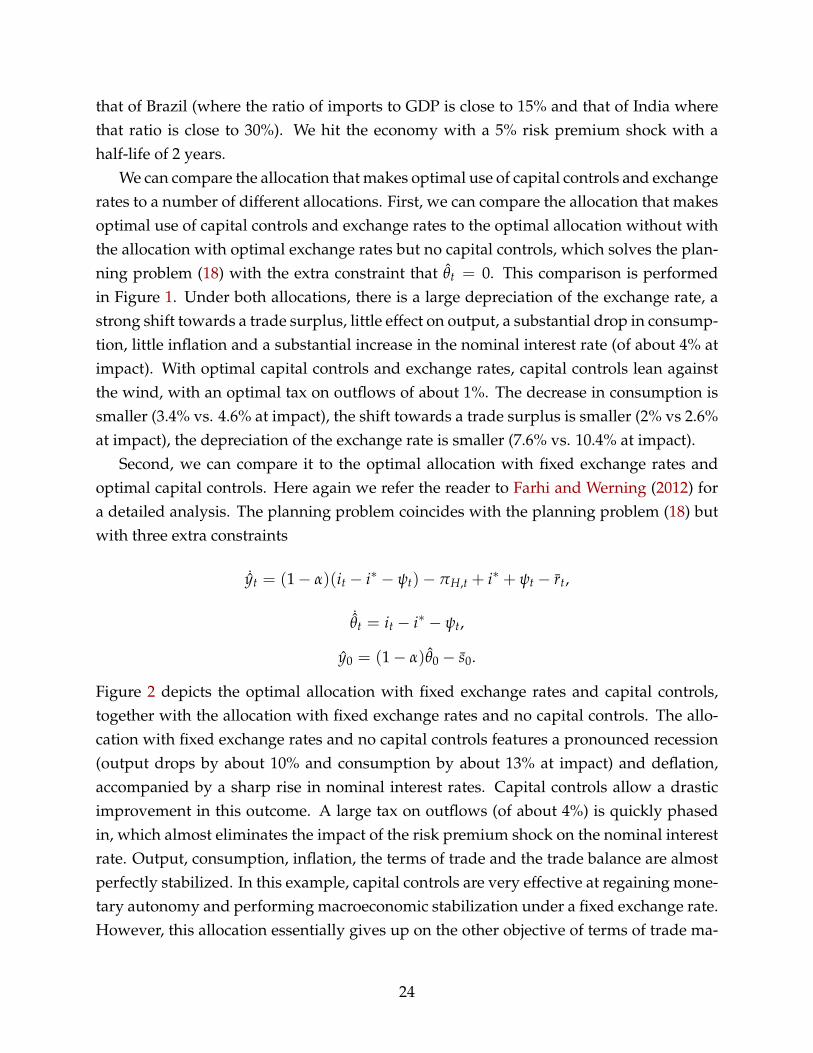
Second, we can compare it to the optimal allocation with fixed exchange rates andoptimal capital controls. Here again we refer the reader to Farhi and Werning (2012) fora detailed analysis. The planning problem coincides with the planning problem (18) butwith three extra constraints

˙yt = (1− α)(it − i∗ − ψt)− πH,t + i∗ + ψt − rt,

˙θt = it − i∗ − ψt,

y0 = (1− α)θ0 − s0.

Figure 2 depicts the optimal allocation with fixed exchange rates and capital controls,together with the allocation with fixed exchange rates and no capital controls. The allo-cation with fixed exchange rates and no capital controls features a pronounced recession(output drops by about 10% and consumption by about 13% at impact) and deflation,accompanied by a sharp rise in nominal interest rates. Capital controls allow a drasticimprovement in this outcome. A large tax on outflows (of about 4%) is quickly phasedin, which almost eliminates the impact of the risk premium shock on the nominal interestrate. Output, consumption, inflation, the terms of trade and the trade balance are almostperfectly stabilized. In this example, capital controls are very effective at regaining mone-tary autonomy and performing macroeconomic stabilization under a fixed exchange rate.However, this allocation essentially gives up on the other objective of terms of trade ma-

24

nipulation.Finally, we can compare it to the flexible price allocation, with optimal capital controls,

which can be implemented with an appropriate exchange rate policy. This comparison isperformed in Figure 3. We find that these two allocations are quite close, except in thevery short run. In other words, the although the perfect dichotomy that we identifiedin Proposition 4 does not hold perfectly, it is not a bad approximation. Under both al-locations, there is a large depreciation of the exchange rate (close to 8%), a strong shifttowards a trade surplus (of the order of 2%), little effect on output, a substantial dropin consumption (approximately 3%), little inflation and a substantial rise in the nominalinterest rate. Optimal capital controls lean against the wind, with an optimal tax on out-flows of about 1%. Most of the difference between the two allocations occurs in the shortrun in the first 6 months of the shock. Under the optimal allocation, the exchange rateand the terms of trade depreciates a little less, consumption drops a little more, the tradebalance shifts towards a slightly larger surplus. The biggest difference is that the optimaltax on outflows is initially substantially smaller and the increase in the domestic interestrate is initially substantially larger.8

5 Conclusion

We have found that both capital controls and flexible exchange rates are important toolsto respond to sudden stops, modeled as risk premium shocks. Flexible exchange ratesare perhaps the most important of the two. The ability to let the exchange rate depreciatedrastically mitigates the consequences of the sudden stop and avoids a large recession.With fixed exchange rates, capital controls have an important macroeconomic stabiliza-tion role to play to regain some monetary autonomy and mitigate the impact of the re-cession. But capital controls also have an important yet different role to play when theexchange rate is flexible. They allow to better navigate the dual objective of macroeco-nomic stabilization and terms of trade manipulation. They help mitigate the depreciationof the exchange rate and of the terms of trade, the drop in consumption, the outflow ofcapital and the associated trade surplus.

In future work, we intend to study capital controls in hybrid models that incorporatepecuniary externalities and nominal rigidities. Such models incorporate more details on

8The relative magnitudes of the increase in the nominal interest rate under both allocations can appearsurprising to the naked eye. Both are however consistent with UIP (modified by the risk premium andthe capital controls). Under the optimal allocation, the tax on outflows and the rate of appreciation of theexchange rate are smaller, enough to require this large difference in interest rates.

25

the finance side of the model and offer a different rationale for terms of trade manipula-tion, namely financial stability.

References

Bianchi, Javier, “Overborrowing and Systemic Externalities in the Business Cycle,” Amer-ican Economic Review, December 2011, 101 (7), 3400–3426.

and Enrique G. Mendoza, “Overborrowing, Financial Crises and ’Macro-prudential’Taxes,” NBER Working Paper 16091 June 2010.

Black, Stanley, “International Money Markets and Flexible Exchange Rates,” Studies inInternational Finance, 1973, (25).

Caballero, Ricardo J. and Arvind Krishnamurthy, “Smoothing sudden stops,” Journal ofEconomic Theory, November 2004, 119 (1), 104–127.

Calvo, Guillermo A., “Capital Flows and Capital-Market Crises: The Simple Economicsof Sudden Stops,” Journal of Applied Economics, November 1998, 0, 35–54.

Cole, Harold L. and Maurice Obstfeld, “Commodity Trade and International Risk Shar-ing: How Much Do Financial Markets Matter?,” Journal of Monetary Economics, 1991, 28(1), 3–24.

Costinot, Arnaud, Guido Lorenzoni, and Ivan Werning, “A Theory of Capital Controlsas Dynamic Terms-of-Trade Manipulation,” NBER Working Papers 17680 December2011.

Devereux, Michael B. and Charles Engel, “Monetary Policy in the Open Economy Revis-ited: Price Setting and Exchange-Rate Flexibility,” Review of Economic Studies, October2003, 70 (4), 765–783.

Farhi, Emmanuel and Ivan Werning, “Dealing with the Trilemma: Optimal Capital Con-trols with Fixed Exchange Rates,” NBER Working Papers 18199, National Bureau ofEconomic Research, Inc June 2012.

Gali, Jordi and Tommaso Monacelli, “Monetary Policy and Exchange Rate Volatility ina Small Open Economy,” Review of Economic Studies, 07 2005, 72 (3), 707–734.

and , “Optimal monetary and fiscal policy in a currency union,” Journal of Interna-tional Economics, September 2008, 76 (1), 116–132.

26

Jeanne, Olivier and Anton Korinek, “Excessive Volatility in Capital Flows: A PigouvianTaxation Approach,” American Economic Review, May 2010, 100 (2), 403–407.

Korinek, Anton, “The New Economics of Prudential Capital Controls: A ResearchAgenda,” IMF Economic Review, August 2011, 59 (3), 523–561.

Kouri, Pentti, “The Exchange Rate and the Balance of Payment in the Short Run and inthe Long Run: A Monetary Approach,” The Scandinavian Journal of Economics, 1976, 78(2), 280–304.

Mendoza, Enrique G., “Sudden Stops, Financial Crises, and Leverage,” American Eco-nomic Review, December 2010, 100 (5), 1941–66.

Obstfeld, Maurice and Kenneth Rogoff, “Exchange Rate Dynamics Redux,” Journal ofPolitical Economy, June 1995, 103 (3), 624–60.

Rey, Helene, “Dilemma not trilemma: the global cycle and monetary policy indepen-dence,” Proceedings, 2013.

Schmitt-Grohe, Stephanie and Martin Uribe, “Prudential Policies for Peggers,” NBERWorking Papers 18031, National Bureau of Economic Research, Inc June 2012.

27

0 1 20

0.05

0.1

0.15e

0 1 2−0.05

−0.04

−0.03

−0.02

−0.01c

0 1 20

0.002

0.004

0.006y

0 1 20

0.05

0.1

0.15s

0 1 2

0

−0.005

−0.01

−0.015

τ

0 1 20.04

0.05

0.06

0.07

0.08i

0 1 20

0.01

0.02

0.03nx

0 1 2−0.006

−0.004

−0.002

0

0.002πH

Figure 1: Capital controls (blue) and no capital controls (green) with flexible exchangerates.

28

0 1 2−1

−0.5

0

0.5

1e

0 1 2−0.2

−0.15

−0.1

−0.05

0c

0 1 2−0.15

−0.1

−0.05

0

0.05y

0 1 2−0.05

0

0.05

0.1s

0 1 2−0.06

−0.04

−0.02

0

0.02τ

0 1 20.02

0.04

0.06

0.08

0.1i

0 1 20

0.01

0.02

0.03nx

0 1 2−0.3

−0.2

−0.1

0

0.1πH

Figure 2: Capital controls (blue) and no capital controls (green) with fixed exchange rates.

29

0 1 20

0.05

0.1

0.15e

0 1 2−0.04

−0.03

−0.02

−0.01c

0 1 20

0.002

0.004

0.006y

0 1 20.02

0.04

0.06

0.08s

0 1 2−0.015

−0.01

−0.005

0τ

0 1 20.04

0.05

0.06

0.07

0.08i

0 1 20

0.01

0.02nx

0 1 2−0.006

−0.004

−0.002

0

0.002πH

Figure 3: Optimal capital controls and exchange rates (blue) and capital controls andexchange rates that replicate the flexible price allocation with optimal capital controls(green).

30

A Appendix

A.1 Derivation of the Loss Function

We focus on Cole-Obstfeld case σ = γ = η = 1. We have the exact relationship

ct = θt + c∗t + (1− α)st

and the following second order approximation of the goods market clearing conditionYt = StC∗t [(1− α)Θt + α]:

yt = c∗t + st + (1− α)θt +12

α(1− α)θ2t .

Using these equations, we can derive

ct = αc∗t + θtα(2− α) + (1− α)yt +12− α(1− α)2θ2

t .

Hence in gaps,

ct = (1− α)yt + α(2− α)θt +12(1− α)2 [−αθt(θt + 2θt)

].

We can use this expression to derive

log Ct = ct + ct

= ct + (1− α)yt + α(2− α)θt − α12(1− α)2θt(θt + 2θt).

We haveN1+φ

t1 + φ

=N1+φ

t1 + φ

+ N1+φt

[yt + zt +

12(1 + φ)y2

t

],

where

zt = logˆ (

PH,t(j)PH,t

)−ε

≈ ε

2σ2

pH,t.

Using the fact that N1+φt = (1− α)(1− αθt) for all t, we get the following expression

31

for the objective function:

ˆ ∞

0e−ρt

(Ut − Ut

CUc

)dt =

− (1−α)(1+φ)2

ˆ ∞

0e−ρt

[αππ2

H,t + y2t −

2α

1 + φytθt

− 2α(2−α)(1−α)(1+φ)

θt + α 1−α1+φ αθt(θt + 2θt)

]dt,

where απ = ε/[λ(1 + φ)].We now use a second order approximation of the country budget constraint to replace

the linear term in θt in the expression above. We find that a second order approximationfor nxt:

nxt = −α(θt +12 θ2

t ).

A first order approximation of the discount factor e−ρte−´ t

0 ψtdt is e−ρt [1 + θ0 − θt].

Combining the two, we get the following second order approximation for the budgetconstraint

α

ˆ ∞

0e−ρt(θt +

12

θt(θt + 2θt) + (θ0 − θt)θt) = 0,

so that we can replace the linear term in θt in the expression for welfare to get the follow-ing expression for the loss function:

(1− α)(1+φ)

ˆe−ρt

[12

αππ2H,t +

12

yt(yt −2α

1 + φθt) +

12

αθ θt(θt + 2(αψθt + (1− αψ)θ0))

]dt,

or up to a constant

(1− α)(1 + φ)

ˆe−ρt

[12

αππ2H,t +

12(yt −

α

1 + φθt)

2 +12

αθ(θt + αψθt + (1− αψ)θ0)2]

dt,

whereαψ =

1− α2−α1−α + 1− α

and αθ =α

1 + φ

(2− α

1− α+ 1− α

).

A.2 Proof of Proposition 5

With flexible prices, we have yt = − α1+φ θt and we can drop the initial condition since the

price of home goods can jump. Hence we are led to the planning problem

min{θt}

12

ˆ ∞

0e−ρt

[(α

1 + φ

)2

(−θt − θt)2 + αθ(θt + αψθt + (1− αψ)θ0)

2

]dt

32

subject to ˆ ∞

0e−ρtθtdt = 0.

Let Γ be the multiplier on the budget constraint. The solution is given by[(α

1 + φ

)2

+ αθ

]θt = −

[(α

1 + φ

)2

+ αθαψ

]θt − αθ(1− αψ)θ0 − Γ.

Since´ ∞

0 e−ρtθtdt = 0 we find Γ = −αθ(1− αψ)θ0 so that the solution is

θt = −( α

1+φ )2 + αθαψ

( α1+φ )

2 + αθθt,

yt =α

1 + φ

( α1+φ )

2 + αθαψ

( α1+φ )

2 + αθθt.

A.3 Proof of Proposition 6

The problem simplifies to

min{yt,θt}

12

ˆ ∞

0e−ρt

[(yt −

α

1 + φθt)

2 + αθ(θt + αψθt + (1− αψ)θ0)2]

dt

subject to ˆ ∞

0e−ρtθtdt = 0.

The solution is yt =α

1+φ θt and θt = −αψθt, which implies

τt = −αψψt.

We can also compute et. For that we use

˙yt = (1− α)(it − ρ) + α(et + ψt)−αφ

1 + φψt,

˙θt = (it − ρ)− (et + ψt),

y0 = (1− α)θ0 + e0 − s0.

This yieldset = −(1− α)(1− αψ)θt,

33

i.e.

et = −(1− α)(1− αψ)

[ˆ t

0ψsds−

ˆ ∞

0ψse−ρsds

],

Hence in response to a negative risk premium shock that mean reverts to zero, the ex-change rate initially appreciates and then depreciates over time.

We can compare the solution to the flexible price solution

τt = −( α

1+φ )2 + αθαψ

( α1+φ )

2 + αθψt,

so that we see that capital controls are always used less with rigid prices and flexibleexchange rate than with flexible prices. However, this difference disappears when α→ 0.

A.4 Proof of Proposition 7

We have

min{πH,t,yt,θt}

12

ˆ ∞

0e−ρt

[αππ2

H,t + (yt −α

1 + φθt)

2 + αθ(θt + αψθt + (1− αψ)θ0)2]

dt

subject toπH,t = ρπH,t − κyt − λαθt,ˆ ∞

0e−ρtθtdt = 0.

The FOCs are−µπ,t = αππH,t,

yt −α

1 + φθt − κµπ,t = 0,

αθ(θt + αψθt + (1− αψ)θ0) + Γ− λαµπ,t = 0.

Note that this implies the following formula for capital controls

τt = −αψψt +λα

αθµπ,t = −αψψt −

λα

αθαππH,t.

This formula depends on the endogenous object πH,t which we determine in closed formbelow.

34

We have the following system of differential equations

πH,t = ρπH,t −(

κ2 +(λα)2

αθ

)µπ,t + λα

[Γαθ− (1− αψ)θt + (1− αψ)θ0

],

µπ,t = −αππH,t,

with µπ,0 = 0. We can differentiate the first equation and use the second to substitute outµπ,t. We find

d2πH,t

dt= ρ

dπH,t

dt+

(κ2 +

(λα)2

αθ

)αππH,t − λα(1− αψ)ψt.

The characteristic polynomial of this differential equation has exactly one negative eigen-value ν− and one positive eigenvalue ν+ where

ν− =ρ−

√ρ2 + 4απ

(κ2 + (λα)2

αθ

)2

and ν+ =ρ +

√ρ2 + 4απ

(κ2 + (λα)2

αθ

)2

.

The solution is of the form

πH,t = λ−eν−t + x+ˆ ∞

te−ν+(s−t)ψsds + x−

ˆ t

0e−ν−(s−t)ψsds.

We have

dπH,t

dt= ν−λ−eν−t − x+ψt + ν+x+

ˆ ∞

te−ν+(s−t)ψsds + x−ψt + ν−x−

ˆ t

0e−ν−(s−t)ψsds.

d2πH,t

dt2 = (ν−)2λ−eν−t − x+dψt

dt− ν+x+ψt + (ν+)2x+

ˆ ∞

te−ν+(s−t)ψsds

+ x−dψt

dt+ ν−x−ψt + (ν−)2x−

ˆ t

0e−ν−(s−t)ψsds.

Hence

d2πH,t

dt− ρ

dπH,t

dt−(

κ2 +(λα)2

αθ

)αππH,t = (x−− x+)

dψt

dt+(ν−x−− ν+x+)ψt− ρ(x−− x+)ψt.

We need

−λα(1− αψ)ψt = (x− − x+)dψt

dt+ (ν−x− − ν+x+)ψt − ρ(x− − x+)ψt,

35

Hence we must havex− = x+,

(ν− − ρ)x− − (ν+ − ρ)x+ = −λα(1− αψ).

The solution is

x− = x+ =λα(1− αψ)

ν+ − ν−.

Hence the solution is

πH,t = λ−eν−t +λα(1− αψ)

ν+ − ν−

ˆ ∞

te−ν+(s−t)ψsds +

λα(1− αψ)

ν+ − ν−

ˆ t

0e−ν−(s−t)ψsds.

To determine λ−, we use the requirement that µπ,0 = 0. This implies that

πH,0 = ρπH,0 + λαΓαθ

.

Using

πH,0 = ν−λ− + ν+λα(1− αψ)

ν+ − ν−

ˆ ∞

0e−ν+tψtdt,

πH,0 = λ− +λα(1− αψ)

ν+ − ν−

ˆ ∞

0e−ν+tψtdt,

this can be rewritten as

(ν− − ρ)λ− + (ν+ − ρ)λα(1− αψ)

ν+ − ν−

ˆ ∞

0e−ν+tψtds = λα

Γαθ

.

This determines Γ as a function of λ−. We then use

αθ(θt + αψθt + (1− αψ)θ0) + Γ− λαµπ,t = 0.

Integrating and using the country budget constraint, we find that

αθ(1− αψ)

ρθ0 +

1ρ

Γ− λα

ˆ ∞

0e−ρtµπ,tdt = 0.

Integrating the last equation by parts using µπ,0 = 0, we can rewrite this as

αθ(1− αψ)

ρθ0 +

1ρ

Γ− λα

ρ

ˆ ∞

0e−ρtµπ,tdt = 0.

36

Using µπ,t = −αππH,t, we can rewrite this as

αθ(1− αψ)

ρθ0 +

1ρ

Γ +λααπ

ρ

ˆ ∞

0e−ρtπH,tdt = 0,

which holds if and only if

αθ(1− αψ)

ρθ0 +

1ρ

Γ +λααπ

ρ

λ−

ρ− ν−+

λααπ

ρ

λα(1− αψ)

ν+ − ν−

ˆ ∞

0e−ρtˆ ∞

te−ν+(s−t)ψsdsdt

+λααπ

ρ

λα(1− αψ)

ν+ − ν−

ˆ ∞

0e−ρtˆ t

0e−ν−(s−t)ψsdsdt = 0,

i.e.

αθ(1− αψ)

ρθ0 +

1ρ

Γ+λααπ

ρ

λ−

ρ− ν−+

1ρ

λ2α2απ(1− αψ)

ν+ − ν−

ˆ ∞

0

[e−ρt − e−ν+t

ν+ − ρ+

e−ρt

ρ− ν−

]ψtdt = 0,

i.e.

αθ(1− αψ)θ0 + Γ+λααπλ−

ρ− ν−+

λ2α2απ(1− αψ)

ν+ − ν−

ˆ ∞

0

[e−ρt − e−ν+t

ν+ − ρ+

e−ρt

ρ− ν−

]ψtdt = 0,

or

Γ = −αθ(1− αψ)θ0 − λααπλ−

ρ− ν−−

λ2α2απ(1− αψ)

ν+ − ν−

ˆ ∞

0

[e−ρt − e−ν+t

ν+ − ρ+

e−ρt

ρ− ν−

]ψtdt,

or

Γ = −αθ(1− αψ)θ0 − λααπλ−

ρ− ν−−

λ2α2απ(1− αψ)

ν+ − ν−

ˆ ∞

0

[− e−ν+t

−ν−+

ν+ − ν−

−ν−ν+e−ρt

]ψtdt.

Together with

(ν− − ρ)λ− + (ν+ − ρ)λα(1− αψ)

ν+ − ν−

ˆ ∞

0e−ν+tψtdt = λα

Γαθ

,

37

this represents a linear system of two equations in two unknowns in Γ and λ−. We find

(ν− − ρ +λ2α2

αθαπ

1ρ− ν−

)λ− = λα(1− αψ)

ˆ ∞

0ψte−ρtdt−

λ3α3απ(1− αψ)

αθ(ν+ − ν−)

ˆ ∞

0

[− e−ν+t

−ν−+

ν+ − ν−

−ν−ν+e−ρt

]ψtdt− (ν+− ρ)

λα(1− αψ)

ν+ − ν−

ˆ ∞

0e−ν+tψtdt.

We can rewrite this as

−ν+ + 1ν+

λ2α2απαθ

λα(1− αψ)λ− =

ˆ ∞

0ψte−ρtdt

− λ2α2απ

αθ(ν+ − ν−)

ˆ ∞

0

[− e−ν+t

−ν−+

ν+ − ν−

−ν−ν+e−ρt

]ψtdt + ν−

1ν+ − ν−

ˆ ∞

0e−ν+tψtdt,

or

ν+ − 1ν+

λ2α2απαθ

λα(1− αψ)λ− =

−ν− − λ2α2απ−ν−αθ

ν+ − ν−

ˆ ∞

0e−ν+tψtdt−

[1− λ2α2απ

−ν−ν+αθ

] ˆ ∞

0ψte−ρtdt.

This gives us λ−. To find the whole solution, we then solve the differential equation

µπ,t = −αππH,t,

with initial condition µπ,0 = 0.From this we get yt from

yt −α

1 + φθt − κµπ,t = 0,

and θt fromπH,t = ρπH,t − κyt − λαθt.

Consider the case where ψt = ψ0e−ρψt. We then have

Γ+λααπλ−

ρ− ν−= αθ(1− αψ)

ψ0

ρ + ρψ−

λ2α2απ(1− αψ)

ν+ − ν−ψ0

[1

ν−1

ρψ + ν++

ν+ − ν−

−ν−ν+1

ρ + ρψ

],

λαΓαθ

+ ν+λ− = −ν−λα(1− αψ)

ν+ − ν−ψ0

ρψ + ν+,

38

which gives us Γ and λ−1. Then we have

−µπ,t

απ= λ−

eν−t − 1ν−

+λα(1− αψ)

ν+ − ν−

[ψ0

ρψ + ν+1− e−ρψt

ρψ+

ψ0

ρψ + ν−

(eν−t − 1

ν−− 1− e−ρψt

ρψ

)],

yt =α

1 + φ

(− ψ0

ρψ + ρ+

ψ0(1− e−ρψt)

ρψ

)+ κµπ,t,

θt = −αψ

(− ψ0

ρψ + ρ+

ψ0(1− e−ρψt)

ρψ

)+ (1− αψ)

ψ0

ρψ + ρ− Γ

αθ+

λα

αθµπ,t.

We can back out the terms of trade from

st = yt − (1− α)θt −1 + φ(1− α)

1 + φ

(− ψ0

ρψ + ρ+

ψ0(1− e−ρψt)

ρψ

).

Finally inflation is

πH,t = λ−eν−t +λα(1− αψ)

ν+ − ν−ψ0e−ρψt

ρψ + ν++

λα(1− αψ)

ν+ − ν−ψ0(eν−t − e−ρψt)

ρψ + ν−.

and the exchange rate from

et = st +

ˆ t

0πH,sds

= st + λ−eν−t − 1

ν−+

λα(1− αψ)

ν+ − ν−ψ0

ρψ + ν+1− e−ρψt

ρψ+

λα(1− αψ)

ν+ − ν−ψ0

ρψ + ν−(

eν−t − 1ν−

− 1− e−ρψt

ρψ).

We can also write

st = ˙yt − (1− α) ˙θt −1 + φ(1− α)

1 + φψ0e−ρψt,

˙yt =α

1 + φψ0e−ρψt − καππH,t,

so thatst = −καππH,t − (1− α) ˙θt − (1− α)ψ0e−ρψt,

et = (1− καπ)πH,t − (1− α) ˙θt − (1− α)ψ0e−ρψt,

it = ρ + ψt +˙θt + et = ρ + (1− καπ)πH,t + α ˙θt + αψ0e−ρψt.

39

We now solve for the optimal allocation without capital controls. We have

min{πH,t,yt}

12

ˆ ∞

0e−ρt

[αππ2

H,t + (yt −α

1 + φθt)

2 + αθ(αψθt + (1− αψ)θ0)2]

dt

subject toπH,t = ρπH,t − κyt.

The FOCs are−µπ,t = αππH,t,

yt −α

1 + φθt − κµπ,t = 0.

We have the following system of differential equations (using κ = λ(1 + φ)):

πH,t = ρπH,t − κ2µπ,t − λαθt,

µπ,t = −αππH,t,

with µπ,0 = 0. We can differentiate the first equation and use the second to substitute outµπ,t. We find

d2πH,t

dt= ρ

dπH,t

dt+ κ2αππH,t − λαψt.

The characteristic polynomial of this differential equation has exactly one negative eigen-value ν− and one positive eigenvalue ν+ where

ν− =ρ−

√ρ2 + 4απκ2

2and ν+ =

ρ +√

ρ2 + 4απκ2

2.

The solution is of the form

πH,t = λ−eν−t +λα

ν+ − ν−

ˆ ∞

te−ν+(s−t)ψsds +

λα

ν+ − ν−

ˆ t

0e−ν−(s−t)ψsds.

To determine λ−, we use the requirement that µπ,0 = 0. This implies that

πH,0 = ρπH,0 − λαθ0.

Using

πH,0 = ν−λ− + ν+λα

ν+ − ν−

ˆ ∞

0e−ν+tψtdt,

40

πH,0 = λ− +λα

ν+ − ν−

ˆ ∞

0e−ν+tψtdt,

this can be rewritten as

(ν− − ρ)λ− + (ν+ − ρ)λα

ν+ − ν−

ˆ ∞

0e−ν+tψtds = −λαθ0,

which determines λ−. We can then determine yt using

κyt = ρπH,t − πH,t.

We have

πH,t = λ−eν−t +λα

ν+ − ν−

ˆ ∞

te−ν+(s−t)ψsds +

λα

ν+ − ν−

ˆ t

0e−ν−(s−t)ψsds,

dπH,t

dt= ν−λ−eν−t + ν+

λα

ν+ − ν−

ˆ ∞

te−ν+(s−t)ψsds + ν−

λα

ν+ − ν−

ˆ t

0e−ν−(s−t)ψsds.

We find

yt = (ρ− ν−)λ−

κeν−t +(ρ− ν+)

λακ

ν+ − ν−

ˆ ∞

te−ν+(s−t)ψsds+(ρ− ν−)

λακ

ν+ − ν−

ˆ t

0e−ν−(s−t)ψsds.

We can back out the terms of trade using yt = st − st, and the exchange rate from et =

st +´ t

0 πH,sds.Consider the case where ψt = ψ0e−ρψt. We then have

(ν− − ρ)λ− + (ν+ − ρ)λα

ν+ − ν−ψ0

ν+ + ρψ= λα

ψ0

ρ + ρψ.

πH,t = λ−eν−t +λα

ν+ − ν−ψ0e−ρψt

ν+ + ρψ+

λα

ν+ − ν−ψ0(eν−t − e−ρψt)

ν− + ρψ,

yt = (ρ− ν−)λ−

κeν−t + (ρ− ν+)

λακ

ν+ − ν−ψ0e−ρψt

ν+ + ρψ+ (ρ− ν−)

λακ

ν+ − ν−ψ0(eν−t − e−ρψt)

ν− + ρψ,

st = yt − ψ01 + φ(1− α)

1 + φ[1− e−ρψt

ρψ− 1

ρ + ρψ],

et = st + λ−eν−t − 1

ν−+

λα

ν+ − ν−ψ0

ν+ + ρψ

1− e−ρψt

ρψ+

λα

ν+ − ν−ψ0

ν− + ρψ(

eν−t − 1ν−

− 1− e−ρψt

ρψ).

41

We can also compute

st = ˙yt − ψ0e−ρψt 1 + φ(1− α)

1 + φ,

˙yt =α

1 + φψ0e−ρψt − καππH,t,

so thatst = −καππH,t − (1− α)ψ0e−ρψt,

et = (1− καπ)πH,t − (1− α)ψ0e−ρψt,

it = ρ + ψt + et = ρ + (1− καπ)πH,t + αψ0e−ρψt.

42