Development of Fast Imaging Solar Spectrograph and...
116
A Dissertation for the Degree of Doctor of Philosophy Development of Fast Imaging Solar Spectrograph and Observation of the Solar Chromosphere Department of Astronomy and Space Science Graduate School Chungnam National University By Hyung-Min Park Advisor Jongchul Chae Titular Advisor Yu Yi February 2011
Transcript of Development of Fast Imaging Solar Spectrograph and...

A Dissertation for the Degree of Doctor of Philosophy
Development of Fast Imaging Solar
Spectrograph and Observation of the Solar
Chromosphere
Department of Astronomy and Space Science
Graduate School
Chungnam National University
By
Hyung-Min Park
Advisor Jongchul ChaeTitular Advisor Yu Yi
February 2011

Development of Fast Imaging Solar
Spectrograph and Observation of the Solar
Chromosphere
Advisor Jongchul ChaeCo-advisor Kyung-Suk Cho
Titular Advisor Yu Yi
Submitted to the Graduate School
in Partial Fulfillment of the Requirements
for the Degree of
Doctor of Philosophy
October, 2010
Department of Astronomy and Space Science
Graduate School
Chungnam National University
By
Hyung-Min Park


To Approve the Submitted Dissertation
for the Degree of Doctor of Philosophy
By Hyung-Min Park
Title: Development of Fast Imaging Solar Spectrograph
and Observation of the Solar Chromosphere
December 2010
Committee Chair Dr. Kap-Soo Oh
Chungnam National University
Committee Dr. Yu Yi
Chungnam National University
Committee Dr. Soo-Chang Rey
Chungnam National University
Committee Dr. Jongchul Chae
Seoul National University
Committee Dr. Kyung-Suk Cho
Korea Astronomy and Space Science Institute
Graduate School
Chungnam National University


Abstract
Traditionally, solar observations have been performed by ground-based in-
struments. Next to the photosphere, the solar chromosphere has been stud-
ied well for a long time. It is well known from high-resolution observations
that chromospheric features are fine structured, short lived, and dynamic. In
obtaining physical parameters, spectrograph-based observations are more ef-
fective than filter-based observations. Through imaging spectroscopy using
a spectrograph, chromospheric features and dynamics can be revealed. The
biggest telescope, New Solar Telescope (NST), was recently built at Big Bear
Solar Observatory. NST has a capability of high spatial resolution, 0.08′′ at
500nm, with the aid of Adaptive Optics. As one post-focus instrument of NST,
an imaging spectrograph, called Fast Imaging Solar Spectrograph (FISS) was
proposed and constructed by Korean researchers to study the solar chromo-
sphere.
This thesis mainly describes our contribution to the development of this
spectrograph and early results. FISS is a grating-based spectrograph with
high spectral resolution, high time cadence, and the capability of imaging. It
has a mount of Littrow type, records dual bands simultaneously, and uses an
Echelle grating as the disperser and performs imaging using a field scanner.
We describe its optical design and performance estimation. Software devel-
opment, construction and integration of each component were completed in
Korea Astronomy and Space Science Institute. Through tests, we confirmed
that the performance of the spectrograph has come close to our expectation.
After FISS was installed on the vertical table on the Coude room at Big Bear
Solar Observatory, we observed various chromospheric features: active regions,
quiet regions, filaments, prominences and so on.
We determined physical parameters of limb prominences observed by FISS.
By applying a non-linear least square fitting of a radiative transfer model to
the profiles of Hα line and CaII 8542A line, we derived physical parameters
of the prominences. The ranges of temperature and non-thermal velocity are
found to be 7,500 - 13,000 K and 5 - 11km/s, respectively. The maximum
1

temperature of prominences is found to be below 20,000 K. It is expected
that FISS will contribute to revealing fine structures and the dynamics of the
solar chromosphere with high resolution.
2
Contents
1 Introduction 11
1.1 Background . . . . . . . . . . . . . . . . . . . . . . . . . . . . . 11
1.2 New Solar Telescope . . . . . . . . . . . . . . . . . . . . . . . . 13
1.3 Adaptive Optics . . . . . . . . . . . . . . . . . . . . . . . . . . . 17
1.4 Necessity of a New Instrument . . . . . . . . . . . . . . . . . . 18
1.5 Outline . . . . . . . . . . . . . . . . . . . . . . . . . . . . . . . . 19
2 Instrument 21
2.1 Introduction . . . . . . . . . . . . . . . . . . . . . . . . . . . . . 21
2.2 Design Concepts . . . . . . . . . . . . . . . . . . . . . . . . . . 22
2.3 Optical design . . . . . . . . . . . . . . . . . . . . . . . . . . . . 24
2.4 Estimation of spectral parameters . . . . . . . . . . . . . . . . . 25
2.4.1 Theory . . . . . . . . . . . . . . . . . . . . . . . . . . . . 25
2.4.2 Estimation of parameters . . . . . . . . . . . . . . . . . . 29
2.5 Intensity Estimation . . . . . . . . . . . . . . . . . . . . . . . . 29
2.6 Components . . . . . . . . . . . . . . . . . . . . . . . . . . . . . 32
2.6.1 Scanner . . . . . . . . . . . . . . . . . . . . . . . . . . . 34
2.6.2 Slit . . . . . . . . . . . . . . . . . . . . . . . . . . . . . . 35
2.6.3 Collimating/Imaging Mirror . . . . . . . . . . . . . . . . 35
2.6.4 Disperser . . . . . . . . . . . . . . . . . . . . . . . . . . 36
2.6.5 Filter . . . . . . . . . . . . . . . . . . . . . . . . . . . . . 37
2.6.6 CCD Cameras . . . . . . . . . . . . . . . . . . . . . . . . 39
3
2.7 Integration . . . . . . . . . . . . . . . . . . . . . . . . . . . . . . 39
2.7.1 Hardware . . . . . . . . . . . . . . . . . . . . . . . . . . 40
2.7.2 Software . . . . . . . . . . . . . . . . . . . . . . . . . . . 40
2.8 Installation . . . . . . . . . . . . . . . . . . . . . . . . . . . . . 47
3 Test 51
3.1 Configuration of feed optics . . . . . . . . . . . . . . . . . . . . 51
3.2 Laser Test . . . . . . . . . . . . . . . . . . . . . . . . . . . . . . 52
3.3 Sunlight Test . . . . . . . . . . . . . . . . . . . . . . . . . . . . 54
3.4 Conclusion . . . . . . . . . . . . . . . . . . . . . . . . . . . . . . 63
4 Early Observations 65
4.1 Data processing . . . . . . . . . . . . . . . . . . . . . . . . . . . 65
4.2 Sunspots . . . . . . . . . . . . . . . . . . . . . . . . . . . . . . . 67
4.3 Filaments . . . . . . . . . . . . . . . . . . . . . . . . . . . . . . 69
4.4 Active Regions . . . . . . . . . . . . . . . . . . . . . . . . . . . 69
4.5 Quiet Regions . . . . . . . . . . . . . . . . . . . . . . . . . . . . 79
4.6 Prominence . . . . . . . . . . . . . . . . . . . . . . . . . . . . . 79
4.7 Conclusion . . . . . . . . . . . . . . . . . . . . . . . . . . . . . . 79
5 Determination of physical parameters of prominences 83
5.1 Introduction . . . . . . . . . . . . . . . . . . . . . . . . . . . . . 83
5.2 Model of Radiative Transfer . . . . . . . . . . . . . . . . . . . . 85
5.3 Data and Analysis . . . . . . . . . . . . . . . . . . . . . . . . . 86
5.4 Results . . . . . . . . . . . . . . . . . . . . . . . . . . . . . . . 87
5.5 Conclusion . . . . . . . . . . . . . . . . . . . . . . . . . . . . . . 101
6 Conclusion 103
Bibliography 105
4

List of Figures
1.1 Perspective drawing of New Solar Telescope (courtesy by BBSO
website) . . . . . . . . . . . . . . . . . . . . . . . . . . . . . . . 14
1.2 New Solar Telescope. A red square represents the Nasmyth
bench. . . . . . . . . . . . . . . . . . . . . . . . . . . . . . . . . 15
1.3 Speckle reconstruction image of a sunspot (AR1084) with AO
on July 2, 2010 at TiO (706nm) band. . . . . . . . . . . . . . . 16
1.4 The concept of AO. . . . . . . . . . . . . . . . . . . . . . . . . 18
2.1 Optical ray design of FISS by using ZEMAX . . . . . . . . . . 25
2.2 Spot diagrams of Hα and CaII8642 by using ZEMAX . . . . . . 26
2.3 A perspective drawing of FISS . . . . . . . . . . . . . . . . . . 33
2.4 The field scanner . . . . . . . . . . . . . . . . . . . . . . . . . . 34
2.5 The slit . . . . . . . . . . . . . . . . . . . . . . . . . . . . . . . 35
2.6 A collimator/imaging mirror . . . . . . . . . . . . . . . . . . . 36
2.7 An Echelle grating . . . . . . . . . . . . . . . . . . . . . . . . . 37
2.8 Filter transmission of Hα (left) and CaII (right). Dashed lines
represent the wavelength at Hα and CaII8542, respectively. . . 38
2.9 A filter adapter . . . . . . . . . . . . . . . . . . . . . . . . . . . 38
2.10 DV887/DV885 EMCCD. . . . . . . . . . . . . . . . . . . . . . . 40
2.11 Quantum efficiency curves of DV887 (upper) and DV885 (lower) 41
2.12 A layout between hardware connections. In this picture, ’M’
means a motor to move a CCD mount. . . . . . . . . . . . . . 42
2.13 A control program of FISS . . . . . . . . . . . . . . . . . . . . 43
5

2.14 The position of FISS components . . . . . . . . . . . . . . . . . 48
2.15 Installation of FISS on vertical table in BBSO . . . . . . . . . . 49
2.16 AO (left) and FISS (right) in Coude room. . . . . . . . . . . . 50
3.1 Feed optics with the laser. It contains laser, telescope as the
beam collimator, iris, and convex lens. . . . . . . . . . . . . . . 53
3.2 The primary mirror of the coelostat . . . . . . . . . . . . . . . 54
3.3 Enlarged laser spectrogram (upper) and its horizontal profile
(lower). In laser spectrogram, x-direction and y-direction in-
dicate spectral domain and spectral domain, respectively. In
lower plot, a dashed line presents gaussian fitting . . . . . . . . 55
3.4 Efficiency curves of echelle grating at Hα (left) and CaII8542
(right) . . . . . . . . . . . . . . . . . . . . . . . . . . . . . . . . 58
3.5 The solar spectrogram (left) and its line profile (right) for Hα . 59
3.6 Two spectrograms of Hα (left) and CaII8542 (right) at the same
time. . . . . . . . . . . . . . . . . . . . . . . . . . . . . . . . . 59
3.7 Raster scan image of the resolution panel on May 10, 2010. On
right side (square), the distortion appears in vertical direction
because of the fluctuation caused by an airplane. . . . . . . . . 61
3.8 Raster scan images of the Sun constructed at Hα (left) and
CaII8542 (right) on December 14, 2009. Horizontal lines on
CaII8542 image are caused by the CCD anomaly at IR. . . . . . 62
4.1 Examples of raw spectrogram (left top), slit pattern (right top),
processed spectrogram (left bottom), flat pattern (right bottom)
at Hα . . . . . . . . . . . . . . . . . . . . . . . . . . . . . . . . 66
4.2 The comparison of raw data profiles with compressed data pro-
files. In upper row, solid lines and red dashed lines represent raw
data profiles and compressed data profiles at Hα and CaII8542,
respectively. Differences between raw data profiles and com-
pressed data profiles are seen in lower row . . . . . . . . . . . . 68
6
4.3 Scan images of a sunspot observed on June 30, 2010. FOV is
64′′×40′′. Dashed lines represent a position of spectrograms in
Figure 4.4. . . . . . . . . . . . . . . . . . . . . . . . . . . . . . 70
4.4 Sunspot spectrograms of Hα and CaII8542. . . . . . . . . . . . 71
4.5 Sunspot images on July 22, 2010. FOV is 40′′×40′′. . . . . . . . 72
4.6 Speckle reconstruction image of sunspot group (AR 11089) at
TiO band (706nm) on July 22, 2010. . . . . . . . . . . . . . . . 73
4.7 Scan images of quiescent filament on July 29, 2010. FOV is
56′′×40′′. . . . . . . . . . . . . . . . . . . . . . . . . . . . . . . 74
4.8 Scan images of a quiescent filament on July 22, 2010. FOV is
56′′×40′′. . . . . . . . . . . . . . . . . . . . . . . . . . . . . . . 75
4.9 Scan images of a quiescent filament on July 16, 2010. FOV is
64′′×40′′. . . . . . . . . . . . . . . . . . . . . . . . . . . . . . . 76
4.10 Scan images of an active region filament on June 25, 2010. FOV
is 72′′×40′′. . . . . . . . . . . . . . . . . . . . . . . . . . . . . . 77
4.11 Emerging flux region associate with active region on July 22,
2010. FOV is 56′′× 40′′. . . . . . . . . . . . . . . . . . . . . . . 78
4.12 Scan images of quiet region near disk center of the Sun on June
25, 2010. FOV is 64′′×40′′. . . . . . . . . . . . . . . . . . . . . 80
4.13 Hα (upper row) and CaII (lower row) spectrograms taken at the
solar limb and a prominence outside it. . . . . . . . . . . . . . 81
5.1 Hα full disk image on June 30, 2010 in BBSO. Two squares
represent field of view of FISS. . . . . . . . . . . . . . . . . . . 88
5.2 Scan images at Hα, CaII in east (left column) and west limb
prominence (right column) . . . . . . . . . . . . . . . . . . . . 89
5.3 A raw spectrogram (upper) and a correction spectrum sub-
tracted aureole light (lower) at Hα. . . . . . . . . . . . . . . . 89
5.4 Two points at the east prominence of Hα (upper) and CaII8542
(lower) . . . . . . . . . . . . . . . . . . . . . . . . . . . . . . . 90
7

5.5 Fitting results of Hα and CaII8542 on position A (upper row)
and B (lower row). Left column represents Hα profiles and
fittings, while right column shows CaII8542 profiles and fittings. 91
5.6 Fitting results at two positions with τ0-variation. Black, green,
red dashed line represent a spectrum profile from data and fit-
ting results with τ0 of 2.5, 0.3, respectively. Blue dashed lines
present τ0 as free parameters. . . . . . . . . . . . . . . . . . . . 92
5.7 Fitting results in Hα and CaII8542 at both the position A (up-
per) and the position B (lower). . . . . . . . . . . . . . . . . . . 94
5.8 Fitting results in Hα and CaII8542 at both the position A (up-
per) and the position B (lower). . . . . . . . . . . . . . . . . . 95
5.9 Positions of interest with height in the east prominence. . . . . 96
5.10 Temperature variations with height. . . . . . . . . . . . . . . . 97
5.11 Sampling positions of Hα (upper) and CaII (lower) in the east
prominence. . . . . . . . . . . . . . . . . . . . . . . . . . . . . 98
5.12 Doppler width (∆λD(Hα),∆λD(Ca)), temperature, and non-
thermal velocity plot (left) and temperature – non-thermal ve-
locity plot (right) in the east prominence. . . . . . . . . . . . . 98
5.13 Sampling positions in the west prominence. . . . . . . . . . . . 99
5.14 Doppler width (∆λD(Hα),∆λD(Ca)), temperature, and non-
thermal velocity plot (left) and temperature – non-thermal ve-
locity plot (right) in the west prominence. . . . . . . . . . . . . 99
5.15 The position where the line broadening is biggest at Hα (upper)
and CaII8542 (lower). . . . . . . . . . . . . . . . . . . . . . . . 100
8

List of Tables
1.1 NST specification . . . . . . . . . . . . . . . . . . . . . . . . . 17
2.1 Base requirements of FISS . . . . . . . . . . . . . . . . . . . . . 23
2.2 Input parameters for optical design of FISS . . . . . . . . . . . 24
2.3 Input parameters to estimate the performance of FISS . . . . . 30
2.4 Estimation values of FISS throughput . . . . . . . . . . . . . . 31
2.5 Parameters and estimation values to calculate photon counts . 32
2.6 Specifications of CCDs . . . . . . . . . . . . . . . . . . . . . . . 39
3.1 Typical observing parameters . . . . . . . . . . . . . . . . . . . 63
9

10
Chapter 1
Introduction
1.1 Background
The Sun is the closest star from us and it’s only a star whose surface we can
see in detail. The violent activity of the Sun, like flares or CMEs and so on,
may affect the Earth seriously, so the monitoring of solar activity becomes
important.
Phenomena in the solar photosphere such as the variation of sunspot num-
ber have been studied well for a long time. On the other hand, features in
the chromosphere could not be observed except during the total solar eclipse
for a while. The routine observations of the chromosphere became possible
only later with the help of high spectral resolution observations using either
narrowband filters or spectrographs.
What is really annoying in ground observation is the troublesome atmo-
spheric seeing. It makes the shape of an object spread, so it is hard to achieve
high angular resolution. Several ways have been suggested to overcome the
seeing. First of all, selecting a good site is important. In case of nighttime
observations, the site is located at a mountain of high altitude that is far away
from cities to avoid artificial lights. In daytime at such a site, however, it is
easy for the sunlight to heat the ground, so the atmospheric convection near
11

the ground is a serious problem. If a solar observatory is located on a lake,
water keeps the ground cool even during daytime, and hence the air near the
ground can be stable. In reality some solar observatories are located on lakes
including Big Bear Solar Observatory, Udaipur Solar Observatory, Huairou
Solar Observatory, and so on. Another way of overcoming the seeing is to
use the instrument like adaptive optics to compensate for image degradation.
With the use of adaptive optics, one can achieve diffraction-limited resolution.
There are two kinds of solar observing system: filter-based ones and
spectrograph-based ones. In case of filter-based systems, either Fabry-Perot
or Lyot filters are mainly used to successively record light in different narrow
spectral ranges. The main advantage of these systems is that they can take
images of a large field of view quickly, but it takes much time to tune many
wavelengths necessary for the construction of line profiles. Interferometric
BIdimensional Spectrometer (IBIS) is a representative instrument (Cauzzi et
al., 2008). By contrast, a spectrograph-based system can take much spectral
information at a specific position, whereas it takes much time to scan a large
field of view. Multi-Channel Subtractive Double Pass (MSDP) spectrograph,
the CCD imaging spectrograph at the Solar Tower Telescope of Nanjing Uni-
versity, the Mees CCD (MCCD) imaging spectrograph, NRL High Resolution
Telescope and Spectrograph (HRTS) onboard sounding rocket are representa-
tive (Mein, 1977; Mein et al, 1997; Ding et al., 1995; Penn et al., 1991; Dere
et al., 1986).
For a long time, solar observations of highest quality have been performed
at Big Bear Solar Observatory (hereafter, BBSO). This observatory is located
on the Big Bear Lake at high altitude (about 2000m), and now has the biggest
solar telescope in the world. Adaptive optics is being applied to correct at-
mospheric fluctuations, and two instruments using Fabry-Perot etalons will be
installed soon. These instruments are mainly intended to observe the solar
photosphere. We are interested in the study of the chromosphere using our
new spectrograph system that was recently installed at BBSO.
12

1.2 New Solar Telescope
The observation system of BBSO consists of two components: New So-
lar Telescope (hereafter, NST) and post-focus system. Four post-focus
instruments— InfraRed Imaging Magnetograph (IRIM), Visible Imaging Mag-
netograph (VIM), Correlation Tracker (CT), Cryogenic IR Spectrograph and
Filtergraph are already installed or will be installed. NST has two foci: Nas-
myth and Coude. The Nasmyth bench is located on the side of the telescope
(see Figure 1.2). CT and Filtergraph have already been installed on the Nas-
myth bench. Other instruments plan to be installed in the Coude room inside
one floor beneath the telescope. Now two instruments, Adaptive Optics Sys-
tem and FISS have been installed on each vertical table in the Coude room.
Light from the Sun is collected by the telescope and fed into the Adaptive
Optics before FISS.
NST has been installed to replace the old 26-inch telescope. NST is a 1.6
meter diameter, off-axis Gregorian system consisting of a parabolic primary
mirror, and is currently the biggest solar telescope in the world. Details of NST
can be found in Figure 1.1. In order to collect more light and reduce stray light,
it was designed to be off-axis. Detailed specifications are given in Table 1.1.
Although BBSO is located at a good site, it’s hard to achieve diffraction lim-
ited images directly from NST because atmospheric disturbance still affects.
Such images can be obtained with the aid of Adaptive Optics (hereafter, AO)
system and speckle reconstruction process. Speckle reconstruction is used to
high-resolution images from a burst of short-exposure raw images. Figure 1.3
presents a sunspot image obtained by applying AO and speckle reconstruc-
tion. This image is the most detailed ever obtained in visible light. AO will
be described in the next Section briefly.
13

Figure 1.1: Perspective drawing of New Solar Telescope (courtesy by BBSO
website)
14

Figure 1.2: New Solar Telescope. A red square represents the Nasmyth bench.
15
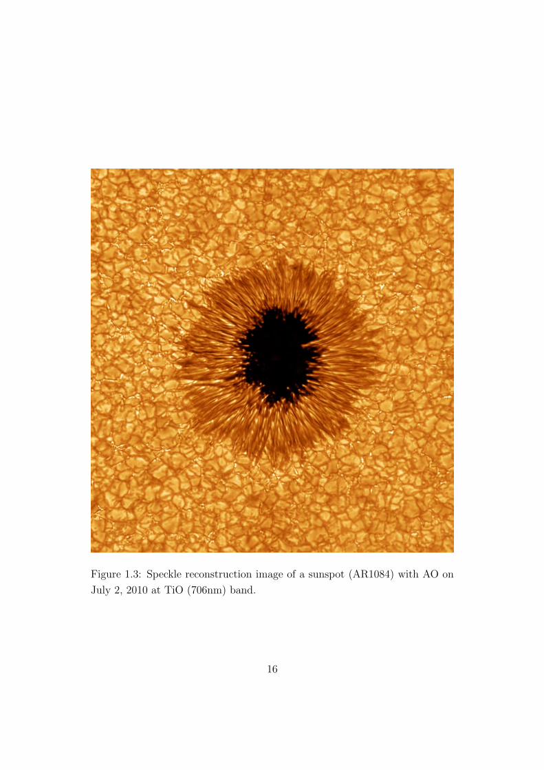
Figure 1.3: Speckle reconstruction image of a sunspot (AR1084) with AO on
July 2, 2010 at TiO (706nm) band.
16

Table 1.1: NST specification
parameters values
clear aperture 1.6 m
effective focal length 83.2 m
wavelength range 0.39-1.6 µm
mounting equatorial mount with friction-based slew
field of view 70′′ × 70′′
diffraction limit 0.08′′ at 500 nm
1.3 Adaptive Optics
Due to inhomogeneities of the atmosphere, image degradation always occurs.
Adaptive Optics is the device of real-time image compensation. Typically an
AO system has three components: wavefront sensor, deformable (adaptive)
mirror, and control system (see Figure 1.4). The disturbance by the seeing
is manifest in the offset positions of sub-images focused by individual lenses
of the lenslet array. Based on sub-images, the control computer calculates
the offsets and send a command to the deformable mirror to correct for them.
Since the atmospheric seeing fluctuates fast, the feedback of AO should operate
at high frequency. Meanwhile, in solar observations, contrary to nighttime
observation, the object we want to see is extended and there is no point sources
available as guides. Alternatively, objects which have high contrast against
background are used as guide sources. For example, the granulation in quiet
regions, sunspots and pores in active regions are good candidates for guide
sources. AO in BBSO is used at two wavelengths, G-band (430.8nm) and TiO
(706nm). Images are better corrected at TiO than G band as AO works better
in IR wavelengths than visible wavelengths.
17
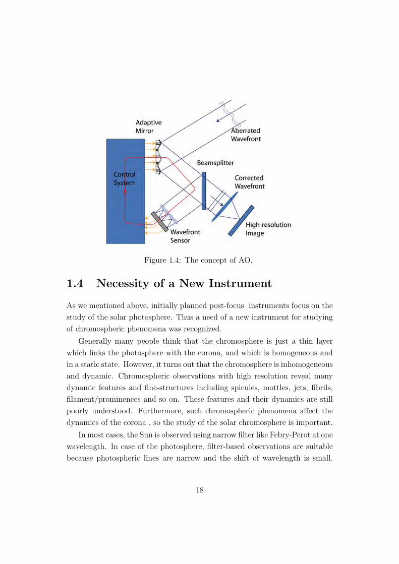
Figure 1.4: The concept of AO.
1.4 Necessity of a New Instrument
As we mentioned above, initially planned post-focus instruments focus on the
study of the solar photosphere. Thus a need of a new instrument for studying
of chromospheric phenomena was recognized.
Generally many people think that the chromosphere is just a thin layer
which links the photosphere with the corona, and which is homogeneous and
in a static state. However, it turns out that the chromosphere is inhomogeneous
and dynamic. Chromospheric observations with high resolution reveal many
dynamic features and fine-structures including spicules, mottles, jets, fibrils,
filament/prominences and so on. These features and their dynamics are still
poorly understood. Furthermore, such chromospheric phenomena affect the
dynamics of the corona , so the study of the solar chromosphere is important.
In most cases, the Sun is observed using narrow filter like Febry-Perot at one
wavelength. In case of the photosphere, filter-based observations are suitable
because photospheric lines are narrow and the shift of wavelength is small.
18
However, if we try to observe the solar chromosphere, a filter-based system is
not suitable anymore because chromospheric lines are broader and line shift
is larger than photospheric lines. For example, we observe violent events such
as filament/prominence eruption, we can see the event while the line centers
are within filter bandwidth. If the speed becomes faster, we may not see the
event anymore since the line centers may be shifted beyond the bandwidth. Of
course, the problem caused by narrow bandwidth can be overcome by tuning
the filter wavelength in series. But this method limits the spectral information
seriously. Thus we came to consider a grating-based spectrograph to see the
solar chromosphere with high spectral resolution, high time resolution, and
high spatial resolution by the aid of NST.
1.5 Outline
This thesis describes our contribution to the development of the new instru-
ment, Fast Imaging Solar Spectrograph, and some early scientific results from
it. Chapter 2 deals with all things of our instrument from concept to instal-
lation and simple theory. Results of lab tests are listed in Chapter 3, and we
will show early observation of the solar chromosphere in Chapter 4. The study
of quiescent prominence observed using FISS is described in Chapter 5.
19

20

Chapter 2
Instrument
2.1 Introduction
The chromosphere, a red color sphere, is a thin layer just above the photosphere
of the Sun. During a total solar eclipse, it can be seen as a thin and red color
layer by a naked eye. It links with the photosphere and corona of the Sun. It
is from the observation of solar chromosphere that hydrogen and helium were
found to be the main chemical constituents.
There are many conspicuous features in the solar chromosphere including
filaments or prominences, plages, active regions, and spicules. The dynam-
ics and structures of these features, however, are not fully understood even
though the solar chromosphere has been observed for a long time. High res-
olution observations have indicated that many chromospheric features have
fine structures that are usually dynamic. For example, filaments/prominences
are known to consist of many thin threads (200 - 1500km width). Threads are
short-lived, and usually contain mass flows along them. To study the fine-scale
structures and dynamics of the chromospheric features, we needs an observing
instrument which should have high angular resolution, high spectral resolution
and high temporal resolution. For high angular resolution, the telescope must
have an aperture which is big enough to reveal fine chromospheric structures
21

in detail.
NST, the biggest telescope in the world, has been constructed at BBSO.
It has the highest spatial resolution we have ever seen, 0.08′′ at 5000A. As we
mentioned in Chapter 1, initially planned observing instruments focus on the
study of the solar photosphere. Accordingly a new instrument to see chromo-
sphere was needed. With this necessity, we have developed the instrument:
the Fast Imaging Solar Spectrograph (FISS).
2.2 Design Concepts
Our scientific goal is to understand physical characteristics of the solar chro-
mosphere, focusing on fine-scale structures and their associated dynamics. For
this we need a spectrograph which has high spatial resolution, high temporal
resolution, and high spectral resolution. Using this instrument, we specifically
want to determine physical parameters such as temperature, density, chemical
composition, and so on. If we observe the Sun at two or more wavelengths
in high spectral order simultaneously, we can estimate several parameters pre-
cisely. Moreover, we can do imaging by moving the solar image across the slit
with fast speed. That is the basic idea of the instrument. To realize the idea,
we have refined the notion of the spectrograph. Spectrograph concepts are as
follows:
• The spectrograph has dual channels to see the solar chromosphere at two
different wavelengths simultaneously. The standard lines to observe the
solar chromosphere are the Hα line and CaII IR line at 8542A. Other
lines such as CaII H & K or HeI in NIR can be used in the single channel
mode.
• A diffraction grating is used as the disperser of the spectrograph. By
using this, we can get spectral data at high spectral resolution with a
large free spectral range.
22

Table 2.1: Base requirements of FISS
Parameters Name Spectrograph Imaging
S/N signal to noise ratio > 102 102
R resolving power > 105 > 3.4× 10⁴
∆x spatial resolution across the slit < 0.2′′ < 0.2′′
∆y spatial resolution along the slit < 0.2′′ < 0.2′′
∆t temporal resolution ≤ 60s ≤ 10s
Ns number of step per scan 600 1200
As scanned area(FOV) 100′′×100′′ 100′′×100′′
• The spectrograph has simple configuration and compact size. If the
spectrograph has simple configuration and small size, it is easy to repair
and maintain.
• The spectrograph has the capability to do imaging. By successively
scanning the position of the slit over the Sun within a short time, it
is possible to do imaging with high cadence. Although the quality of
imaging is poorer than a filtergraph, physical information contained in
the spectra is abundant enough.
To take fast scan, the stabilization has to be ensured. Since NST uses the
AO system to correct for the seeing, we don’t have to care about atmospheric
fluctuation. Meanwhile, a fast camera is essential to obtain a series of spec-
trograms at high cadence. Table 2.1 shows the requirements for observation.
Based on them, we have refined the concept of spectrograph in detail. To
realize general ideas, we drew up guidelines as follows:
• The mounting of FISS is of Littrow type. It allows the spectrograph to
have a simple configuration. Since incident angle and diffraction angle
are close to blaze angle, a single mirror/lens can play as both a collimator
and an imager.
23

Table 2.2: Input parameters for optical design of FISS
Name Parameter Value
F-ratio of incident beam Fi 26
focal length of incident beam fi 41.6m
collimator/image focal length fcol 1.5m
grating groove density d 79/mm
grating blaze angle ϕ 63.4
deflection angle for CCD A α− β 0.93
deflection angle for CCD B α− β 1.92
• An Echelle grating is used as the disperser to get spectra of high spectral
orders. It is suitable for taking the data which have high spectral reso-
lution and wide spectral range. We intend to obtain the data with high
spectral resolution at a specific wavelength band, so a bandpass filter is
adopted to remove the order-overlapping.
• A field scanner is used. The scanner enables the solar image to move
across the slit. With the interlocking between the field scanner and the
detector, we can do imaging. It will operate two ways: imaging mode
and spectrograph mode.
FISS has been designed based on these guidelines. Design parameters are
listed in Table 2.2.
2.3 Optical design
The design has been performed using the optical design program, ZEMAX.
The pair of wavelength, Hα and CaII8542 is considered. A paraboloid mirror
is used as the collimator/imager. Figure 2.1 is the optical layout based on
the design parameters. The light dispersed by the grating is reflected by the
24

Figure 2.1: Optical ray design of FISS by using ZEMAX
paraboloid mirror, and goes into each of two detectors. Figure 2.2 represents
the spot diagrams at Hα and CaII8542, respectively. The circle around each
spot represents the diffraction limit at the wavelength and is larger than the
spot formed by the incident beam. Since the diffraction limit size is propor-
tional to the wavelength, the size of diffraction limit at CaII8542 is larger than
the airy disk at Hα.
2.4 Estimation of spectral parameters
2.4.1 Theory
The diffraction theory starts with the grating equation
mλ = d(sinα + sin β). (2.1)
25
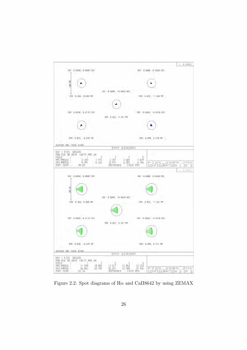
Figure 2.2: Spot diagrams of Hα and CaII8642 by using ZEMAX
26
where m is spectral order, λ, wavelength, d, groove distance between adjacent
grating grids, α, incidence angle, β, diffraction angle, respectively.
In order to understand the spectrograph, spectral order should be calcu-
lated first. FISS uses Littrow mounting, that means incident angle, diffraction
angle and blaze angle of grating are almost the same(α ≃ β ≃ ϕ). Using this
relation, spectral order at specific wavelength can be calculated. The spectral
order, m, is estimated by
m = Rn(2d sinϕ
λ), (2.2)
where ϕ is blaze angle, Rn is the rounding off function that yields the integer
close to the argument.
We introduce the difference between incident angle and diffraction angle,
θ = α − β. Removing β in Equation 2.2 using this expression of θ, we obtain
the non-linear equation for α
sinα + sin(α− ϕ)− mλ
d= 0. (2.3)
This equation can be solved iteratively for α using the Newton-Rapson method.
Linear Dispersion defines the extent to which a spectral interval is spread
out. It represents the ability to resolve fine spectral in detail. The expression
of linear dispersion is as follows:
dλ
dx=
d cos β
mfcam, (2.4)
where fcam is the focal length of camera.
Linear dispersion per pixel is given by
δλ =d cos β
mfcamwdet, (2.5)
where wdet is a pixel size. Based on linear dispersion per pixel, we can estimate
the spectral coverage on CCD chip. Spectral coverage of detector is given by
dλ =d cos β
mfcamWdet, (2.6)
27
where Wdet is the size of detector.
Grating resolution is given by
δλgrating =λd
mWgrating
, (2.7)
where Wgrating is grating width.
Spectral purity measures the degradation by finite slit width. Incident
beam that goes through the slit of finite width contains a finite spread of
the incidence angle and brings about the spread of diffraction angle so that
resolution gets worse. If we want to reduce spectral purity, either the distance
from slit to collimator should be long enough or slit width should be narrow
enough. Spectral purity (spectral resolution of the slit) is as follows:
δλsp = cosαws
fcol
d
m, (2.8)
where ws is slit width, fcol is the distance between slit and collimator.
Detector resolution is given by
δλdet = 2× δxdλ
dx= 2× cos β
δx
fcam
d
m, (2.9)
where δx is a pixel size of detector, fcam is the distance between imager and
detector.
The net spectral resolution before sampling is given by
δλD =√(δλgrating)2 + (δλsp)2, (2.10)
and spectral resolution after sampling by
δλD =√(δλgrating)2 + (δλsp)2 + (δλdet)2. (2.11)
The resolving power is dimensionless, representative value for the spec-
trograph. It is proportional to the smallest difference between specific wave-
lengths. The equation is given by
R =λ
δλD
, (2.12)
where δλD the smallest difference in wavelengths that can be just distinguished.
28
2.4.2 Estimation of parameters
Using relations associated with diffraction theory, spectrograph parameters are
estimated. Input parameters to calculate throughput are listed in Table 2.3.
Table 2.4 shows spectrograph throughput.
2.5 Intensity Estimation
Ahn et al. (2008) estimated the shapes of spectral profiles of Hα and CaII8542
lines and calculated photon counts on the CCD chips. The photon count at
the continuum (Ne) is expressed as follows:
Ne = q · τatm · τins · IC · λ
hν·∆Ω ·∆λ ·∆A ·∆t (2.13)
= q · τatm · τins · ICλ
hc·∆x ·∆y · π
4F 2·∆λ ·∆t,
where ∆ω is solid angle of the telescope, ∆A, unit area, F, focal ratio of incident
beam, respectively. Other parameters and values are listed in Table 2.5.
The photon count in Hα and CaII8542 are 2.51×10⁵, 2.03×10⁵, respec-
tively. If this value is true, Analog-to-digital converting unit(ADU) count on
CCD should be too high to detect all. However photon count obtained by
tests was found to be much lower than these values. Furthermore, the values
obtained at Korea Astronomy and Space Science Institute (hereafter, KASI)
were found to be much different from those taken at BBSO. This discrepancy
between calculation and determination is due to their wrong assumptionon
the instrument transmission. Ahn et al. regarded the instrument transmis-
sion as 0.25. We found that this value was much overestimated. The optical
configuration for NST and AO system has lots of optical surfaces like mirrors
and lens. They didn’t consider the transmission of all the components, mirror,
filter, grating and so on. Instrument transmission calculated again is found
to be about 0.01. Based on this new value, we obtain photon counts of 1.06
×105 and 1.2 ×10³ for Hα and CaII 8542, respectively, corresponding to to
29
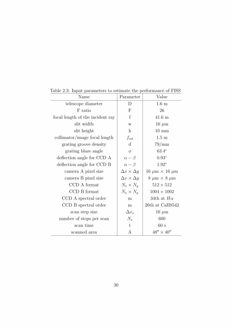
Table 2.3: Input parameters to estimate the performance of FISS
Name Parameter Value
telescope diameter D 1.6 m
F ratio F 26
focal length of the incident ray f 41.6 m
slit width w 16 µm
slit height h 10 mm
collimator/image focal length fcol 1.5 m
grating groove density d 79/mm
grating blaze angle ϕ 63.4
deflection angle for CCD A α− β 0.93
deflection angle for CCD B α− β 1.92
camera A pixel size ∆x×∆y 16 µm × 16 µm
camera B pixel size ∆x×∆y 8 µm × 8 µm
CCD A format Nx ×Ny 512× 512
CCD B format Nx ×Ny 1004× 1002
CCD A spectral order m 34th at Hα
CCD B spectral order m 26th at CaII8542
scan step size ∆xs 16 µm
number of steps per scan Ns 600
scan time t 60 s
scanned area A 48′′ × 40′′
30

Table 2.4: Estimation values of FISS throughput
Name Parameter Hα 6563A CaII 8542A
incidence angle α 62.28 62.28
diffraction angle β 61.34 60.38
spectral order m 34 26
linear dispersion dλ/dx 1.2 mA/µm 1.6 mA/µm
spectral coverage per a pixel δλc 19 mA 26 mA
spectral coverage on chip dλc 9.8 A 12.9 A
grating resolution δλgrating 19.7 mA 33.53 mA
detector resolution δλdet 38.1 mA 51.3 mA
spectral purity δλsp 18.5 mA 24.2 mA
spectral resolution before δλ 27 mA 41 mA
spectral resolving power before λ/δλ 243,000 207,000
spectral resolution after δλ 46 mA 48 mA
spectral resolving power after λ/δλ 141,000 130,000
beam width on grating Wgrating 124 mm
beam height on grating 57.7 mm
31

Table 2.5: Parameters and estimation values to calculate photon counts
Parameter Name Ha CaII8542
q quantum efficiency 0.9 0.35
τatm atmospheric transmissivity 0.699 0.706
∆λ spectral coverage of a pixel (mA) 19 25
IC continuum intensity 2.9 ×10⁶ 1.78 ×10⁶
(erg/cm2/str/sec/A)
Ne photon count of continuum 10629.6 1226.29
N data number (DN) 796 1052
τins instrumental transmissivity 0.011
∆x physical width of a CCD Pixel (µm) 16
∆y Physical height of a CCD Pixel (µm) 16
∆t CCD exposure time (sec) 0.03
F focal ratio of incident beam 26
796 ADU and 1052 ADU, respectively. These values are close to the values
obtained by observations. To enhance instrument transmission, it is necessary
to replace the aluminum mirror coating by the enhanced-silver because the
reflexibility of silver is larger than aluminum.
2.6 Components
Typically, a spectrograph is composed of a slit, a collimator, a disperser, an
imager and a detector. In addition to these, FISS has a field scanner and
bandpass filters. As we mentioned, a portion of paraboloid mirror serves as
both collimator and imager. Figure 2.3 shows the FISS configuration. CCD A
and CCD B are to take spectrograms at Hα and CaII8542, respectively. Each
component is described in this section.
32

Figure
2.3:
Aperspective
drawingof
FISS
33

Figure 2.4: The field scanner
2.6.1 Scanner
Generally Littrow spectrograph uses rotating mirror in front of slit to sweep
an image of luminous object like the Sun. But FISS does not use such a
rotating mirror, and uses instead a field scanner which is composed of two flat
mirrors and a linear stage motor as the movement device. This scanner does
not require a pupil as the location, and hence it makes the optical design of
the instrument much simple. The field scanner installed on the vertical table
is shown in Figure 2.4. It uses JSMD linear motor by Justek and PMAC
Mini board by Delta Tau. The field scanner displays two kinds of motion:
step-by-step motion and linear drift motion. Scanner drifts fast without stop
in imaging mode, while it moves step by step in spectrograph mode. Tests
indicated that moving accuracy is less 1 µm when the scanner moves 16µm
at each step (Ahn, 2009).
34

Figure 2.5: The slit
2.6.2 Slit
The slit was designed and made by KASI. The initial design of the slit width
was 16µm that corresponds to 0.08′′, necessary to achieve the intended spatial
resolution of 0.16′′. Since the amount of light was later found to be insufficient,
the slit width was changed from 16µm to 32µm. The slit is now attached on
the vertical table with its plane facing up, so that dusts on slit surface are one
of the most serious problem. In order to block dusts, a slit cap was installed
in addition. Figure 2.5 presents the slit that we used.
2.6.3 Collimating/Imaging Mirror
FISS uses an off-axis mirror which originates from a portion of paraboloid
mirror. The mirror makes the spectrograph configuration simple, and we don’t
need to concern about chromatic aberration which occurrs in a lens-based
optics system. The mirror mount can control its position in 3 axes. The
mirror is made of zerodur and is coated by enhanced aluminum. It has a
radius of 300mm. Figure 2.6 presents the collimating/imaging mirror.
35

Figure 2.6: A collimator/imaging mirror
2.6.4 Disperser
The disperser is the most important component in the spectrograph. Usually
prism or diffraction grating is used as a disperser. The performance of diffrac-
tion grating depends on groove density and blaze angle. Echelle grating is a
kind of diffraction grating. It is different from normal grating in many ways.
Echelle has low groove density (below 316 grooves/mm), high blaze angle, high
efficiency and wide spectral range. To achieve wide spectral range, a prism is
sometimes used as a cross disperser, but it is not used in our instrument. The
Echelle grating we used is R2 (the tangent of the groove angle, blaze angle of
63.4 ), groove density of 79 grooves/mm and made by Richardson Lab. The
grating surface is coated by aluminum and is overcoated by a thin layer of
magnesium fluoride (MgF2) to prevent the oxidation of the aluminum. We
only use spectral orders of 34th for Hα, 26th for CaII8542, respectively. The
disperser is mounted on a rotating motor which is controlled by a computer. It
enables the grating to fix at or rotate to the specific angle during observation.
The resolution of grating angle is 1.98 ′′/step. This value corresponds to about
1 pixel (16µm) on CCD chip.
36

Figure 2.7: An Echelle grating
2.6.5 Filter
An important limitation of the Echelle grating is order-overlap at high spectral
orders. To avoid this order-overlap, we use bandpass filters.
Free Spectral Range (hereafter, FSR) is defined as a criterion of order su-
perposition. It is the largest wavelength range not to overlap with the spectral
range in an adjacent order. If the (m + 1)th order of the wavelength (λ) and
mth order of λ+∆λ lie at same angle, FSR is as follows:
FSR =λ
m. (2.14)
For example, the FSR is 193A at Hα (λ=6562.8A) and m=34. The higher
the spectral order is, the lower FSR is. If we use the filter whose bandpass is
smaller than FSR, we can observe the specific order that we want. For Hα,
we used bandpass filter whose FWHM is 100A. For CaII8542, FSR is 328A
so that the filter with the FWHM of 250A is used. The transmission curves
of the filters are depicted in Figure 2.8. Dashed lines represent the position
at each wavelength. Filter transmissions at Hα and CaII8542 are 0.66, 0.65,
respectively.
37
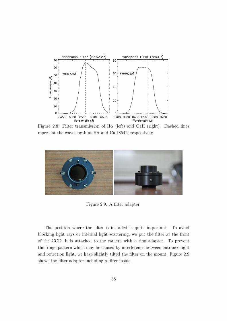
Figure 2.8: Filter transmission of Hα (left) and CaII (right). Dashed lines
represent the wavelength at Hα and CaII8542, respectively.
Figure 2.9: A filter adapter
The position where the filter is installed is quite important. To avoid
blocking light rays or internal light scattering, we put the filter at the front
of the CCD. It is attached to the camera with a ring adapter. To prevent
the fringe pattern which may be caused by interference between entrance light
and reflection light, we have slightly tilted the filter on the mount. Figure 2.9
shows the filter adapter including a filter inside.
38

Table 2.6: Specifications of CCDs
DV887 DV885
CCD Type back-illuminated front-illuminated
active pixels 512 × 512 1004 × 1002
pixel size (µm) 16 8
image area (mm) 8.2 × 8.2 8 × 8
max readout rate (MHz) 10 35
EM Gain 1-1000 1-1000
dynamic range (Bit) 14 14
2.6.6 CCD Cameras
There are many kind of CCD cameras for astronomical observation. However,
it is hard to find the cameras for specific purpose like solar observation. To
catch images of faint and fine structures on the Sun rapidly, a camera should
have high time cadence, high quantum efficiency and low readout noise. To
satisfy these criterion, we selected DV887 for Hα and DV885 CCD for CaII8542
by Andor Company (see Figure 2.10). Main specifications are described in
Table 2.6, and quantum efficiencies are depicted in Figure 2.11. Two cameras
are electron multiplying CCDs (EMCCD) in which a gain register is placed
between the shift register and the output amplifier. The gain register consists
of lots of stages, and the electrons are multiplied in each stage, so that it can
get thousands of electrons from one electron with low readout noise.
2.7 Integration
Integration is the process to collect each component of FISS. Integration pro-
cess contains both connecting hardware components into one and merging each
program to control hardware into one. Two processs are described here.
39

Figure 2.10: DV887/DV885 EMCCD.
2.7.1 Hardware
The operation of FISS is controlled by a computer which connects the scanner,
the slit cover, the grating, the CCD mounts and the CCD cameras. Figure 2.12
shows the diagram of the hardware connection in FISS. Basically a PC controls
the FISS system using onboard PCI cards. In case of the grating, CCD mounts
and scanner control, a servo drive is used to deliver their command from the
PC to the motor. The control boxes for scanner and grating motor have been
constructed in KASI. Each control box includes a power connector and a servo
driver to deliver the command from the computer to each motor. Briefly
speaking, the computer has four PCI cards which are connected to seven parts
of FISS. Electric power is supplied not only to the control boxes but also to
the CCDs separately.
2.7.2 Software
We have developed the control program for each device using the software
development kit (SDK). Each control program is merged into one. After in-
40
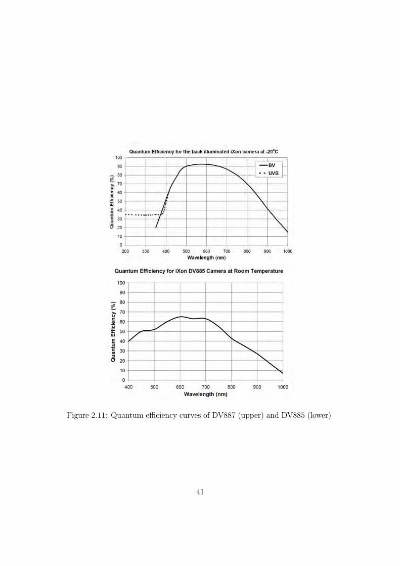
Figure 2.11: Quantum efficiency curves of DV887 (upper) and DV885 (lower)
41

Figure 2.12: A layout between hardware connections. In this picture, ’M’
means a motor to move a CCD mount.
42

Figure 2.13: A control program of FISS
43
tegration of the programs, the program for the observation was developed.
Labwindows/CVI made by National Instruments is used as the software devel-
opment tool. Since CVI contains ansi-C basement and graphic user interface
(GUI) is easier than in MS Visual C++, we could develop the program effi-
ciently at short time.
A program technique commonly used in the FISS control programs is
thread. Thread is the smallest unit of processing that can be scheduled by
an operating system like MS windows. It generally results from a divergence
of a computer program into two or more concurrently running tasks. We used
the thread function for the monitoring of CCD temperature, realtime image
display, and FISS status display. The FISS program is composed of data view
and several controls of the CCD, scanner, and grating/CCD motor.
CCD control The CCD program consists of 2 parts: setting the CCD pa-
rameters and saving data. Parameters of a CCD camera include exposure
time, shutter on/off, cooling on/off, binning and so on. All the parameters
can be controlled mostly by clicking the corresponding button on the GUI
panel. FISS data are saved into files as FITs format. The program saves
data in 2D form for single spectrogram mode and in 3D form for imaging
spectroscopy mode or flat-fileding mode. We used the CFITSIO library from
NASA (HEASARC, 2009). Each data file is named by the universal time of
observation. CCD parameters and other information are recorded in the FITs
header of the data.
After developing basic control program, we have optimized the program to
deal with several problems such as processing speed, memory management, and
controlling of the 2 CCDs. Memory management is crucial in the operation of
FISS. If FISS take a single spectrogram, it needs only a memory size of about
512KB. However we plan to take several hundred frames per one scan, and
the FISS program requires additional memory for data manipulation for the
interactive observation, so that we need much bigger memory. The maximum
size of memory allocable to a 32-bit operating system is about 2.1Gbyte. But
44

we have to keep in mind that the memory that can be used by the FISS
program is much smaller than this because the operating system and other
programs installed on computer occupy a good portion of the total memory.
Controlling 2 CCDs may be another problem. The two CCDs that we use
are from the same manufacturer, and hence we can use the same SDK for both
the cameras (ANDOR, 2009). But there are many differences in pixel number,
size, gain range, affecting the size of memory, data size, window size of viewer,
binning rate and so on. It is also important to have 2 CCDs interlocked.
Scanner control The scanner control program has been developed by using
the PMAC driver (DELTA TAU, 2003). The program has four main functions:
power on/off, making script for command execution, monitoring current status,
and command input. When users input a few parameters on the GUI panel, a
script which includes several commands to move the scanner is created. After
that, commands are sent from the script file to the ROM of PMAC board,
and then the scanner starts to move. They can select one of two kinds of
motions: stepwise motion and continuous motion. In both the cases, the CCD
and the scanner operate at the same time. If the scanner motion is stepwise,
the scanner moves a specific distance and waits until data are taken by the
CCD. In the continuous mode, the scanner moves without stopping, while the
CCD operates regularly. The stepwise and continuous runs of the scanner
correspond to the spectrograph mode and the imaging mode of the FISS.
Grating/CCD motor control Grating and CCD benches are moving
parts, too, hence motor control is necessary. When FISS is turned on, grat-
ing should be positioned at specific angle precisely. Furthermore, controlling
the distance between imager mirror and CCD is essential to focus on clear
object. Then the program of Grating/CCD control has been developed by
using SDK (PARKER, 1998). The Grating/CCD control box connects four
motors, grating motor, CCD focus motors, and slit cap. The program is con-
trolled by a computer using ethernet port. The program mainly consists of
45

five functions, returning home position angle, moving specific angle, checking
the current status, and matching between wavelength and grating angle, and
command input.
Viewer Viewer program consists of 3 contents: display window to view raw
data from CCD or FITs file, scaling bar to see the image in detail, and display
window to view current status of system and setting value, respectively. Data
viewer can display raw data from CCD and FITs file both 2D and 3D. In case
of 3D data, user can select frame number to see and the direction of either
raster image in spectral domain or spectrogram in spatial domain. During
observation, raster image at wavelength center can be displayed on viewer
panel sequentially. After obtaining, we can see either Hα and CaII image by
clicking radio buttons on the panel. By using scaling bar, user can see the
image in detail. If the data is 3D, frame slide bar is activated, hence we can
see spectrogram or raster scan image.
As long as the data is loaded in the display viewer panel, intensity his-
togram appears in graph panel automatically at the same time. As a mouse
curser moves on data viewer panel, horizontal line profile and the mouse cursor
position are displayed at the histogram panel simultaneously. Of course, users
can see histogram when they click the mouse on graph panel.
Parameter viewer display the data number (DN), X and Y position, av-
erage, and standard deviation of the DN. If we read the data from FITs file,
it shows header information written in FITs header. Also parameter viewer
can show setting parameters when we set to FISS. Important parameters are
displayed such as FISS mode, scan step size, time per a scan, exposure time
of the CCD and so on. The status of FISS is checked in lamp color and as
scripts on panel.
Integration with each program All programs to control the individual
components have been integrated. Each program controls its instrument, but
integration is not sufficient for observation program. The program should take
46

into account not only mechanical controlling but also observation condition.
We added several functions into the program to apply for observation.
To take calibration data for bias and dark subtraction, 100 frames are
acquired for each camera with the same exposure time, binning rate, cooling
and so on as real observations, but with the shutter open. Frames are averaged
and then only the average one is stored in hard disk on computer. Bias/dark
is obtained whenever CCD setting is changed.
To get flat/calibration data, the program controls the grating, CCD and
scanner successively or simultaneously. Flat/calibration data are usually taken
before and after observation. When flat fielding mode is chosen for observation,
grating angle is fixed specific angle which locates Hα or CaII8542 line at specific
positions on the corresponding CCDs. A quiet region is scanned so that about
400 frames are obtained. At that position, the averaged one is stored into the
computer. The grating angle changes 7 times and the same process as above is
repeated seven times. As a result, 7-averaged frames are stored in hard disk.
During solar observation, observer may want to record observation condi-
tion like position, target and so on. As an observation log, input panel was
made in integration program. The observation program has the capability
to record observer name, the position what they want to see in heliocentric
coordinate, observation target, active region number on input panel. These
information are recorded in FITs header. Figure 2.13 shows the integration
program to control FISS. Main program hide a few subpanel associate with
setting each component.
2.8 Installation
After completing integration process, we integrated all components on optical
table for tests. In the beginning of installation, each component was installed
on horizontal table in KASI. To attach instruments, the position information
about each device is necessary. Based on design coordinate from ZEMAX,
install position on optical table was decided so that we installed each instru-
47

Figure 2.14: The position of FISS components
ment. Figure 2.14 is the position which is supplied by ZEMAX. According to
drawing, the base point is the slit position. After attachment of the slit, other
instruments are attached successively.
The laser is used as the light source during installation. HeNe laser (6328A)
is very useful to attach and to align instrument precisely. Furthermore, the
wavelength of the laser is close to Hα. After completing to install on horizontal
table, all components are also installed on vertical table. During installing on
vertical table, we found that weight balance of grating is not suitable and
dusts between slit blades affect spectrum quality. Then balance weight on
grating are attached in addition, and slit cap was also installed to protect dust.
After testing in KASI, we transported FISS to BBSO and installed on vertical
table in the Coude room. Meanwhile, cable connection among the device on
the optical table, control boxes, and a computer have been performed. The
control computer, grating control box, and scanner control box were located
in observation room near Coude room. Finally shield case was attached to the
FISS to protect dust and stray light. Figure 2.15 and Figure 2.16 show FISS
on vertical table in the Coude lab.
48
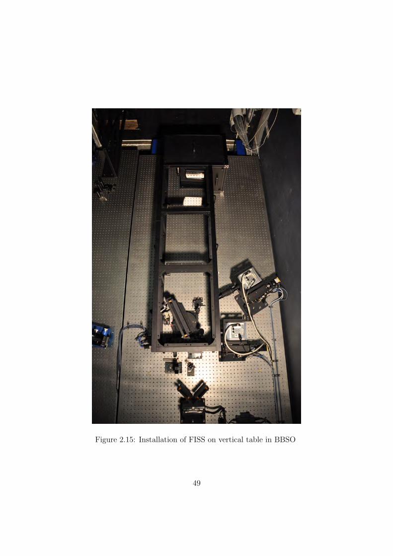
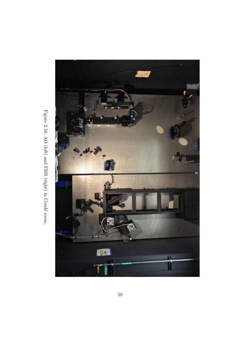
Figure 2.15: Installation of FISS on vertical table in BBSO
49
Figu
re2.16:
AO
(left)an
dFISS(righ
t)in
Cou
deroom
.
50

Chapter 3
Test
After the installation, the instrument was tested mainly at KASI. In order to
supply light to FISS, we set up the feed optics system in front of the spec-
trograph. At the beginning of test, as we mentioned above, a HeNe (6328A)
laser was used as the light source. After the laser test, FISS was tested by
using the sunlight. Through testing, we determined the performance of our
spectrograph. Here we describe the process and results.
3.1 Configuration of feed optics
A light source is needed for testing FISS. The laser and the Sun are used as the
two light sources of the spectrograph. These lights are parallel, so the imager
which converges the lights is essential. The fed light should be F/26 light with
the same F-number as FISS in BBSO. For this, an iris is needed to adjust the
effective aperture of the lens and hence the F-ratio of the converging beam.
A convex lens of 1 meter focal length was used as the imager. The F-ratio
of the imager was adjusted by the iris attached to it (Nah et al., 2009). The
advantage of using the same focal ratio is in the flexibility that lights gathered
by telescopes of different focal lengths and different field of views can be fed
into the same instrument without changing the optical configuration, only if
51

they have the same F-ratio.
When the laser is used as the light source, we need a collimator to convert
the light from the point-like source into a bundle of expanded parallel beam. A
small refraction telescope is used as the collimator. Generally a telescope like
this is used as the light collector. The bundle of light from a distant source is
converged by the object glass and paralleled by the eyepiece to be fed into an
observer’s eye. But we used the telescope in the opposite way by reversing the
direction of light: we put the laser at the original position of the observer’s eye.
The light from the laser then passes through the eyepiece, converges into the
focus, then passes through the objective lens, and finally becomes an expanded
collimated beam. Figure 3.1 is the feed optics consisting of laser, telescope,
iris and convex lens.
Contrary to the laser, the Sun is not stationary on the plane of sky. We
tracked the Sun and feed the sunlight into the laboratory using a coelostat.
The coelostat consists of two rotating mirrors that can always reflect sunlight
along the specified path. With this coelostat, the solar image neither move,
nor rotate even when the Sun moves across the sky. In other words the solar
light is fed into the optical table in a constant direction. Figure 3.2 is the
primary mirror of the coelostat we used.
3.2 Laser Test
There are many reasons why we use a laser as the light source. Since the laser
is bright enough and goes straight with little dispersion on the light path, we
could align all instruments with same height on optical table quickly. Moreover
it is a monochromatic point source; the spectrogram of a laser source taken by
CCD chip is a spot both in the spectral domain and in the spatial domain. This
spot helps us not only in precisely setting the distance between imaging mirror
and each CCD, but also in locating the positions of the CCDs correctly. Once
the alignment of laser is complete, we don’t have to work to change optical
configuration of FISS any longer.
52

Figure 3.1: Feed optics with the laser. It contains laser, telescope as the beam
collimator, iris, and convex lens.
53
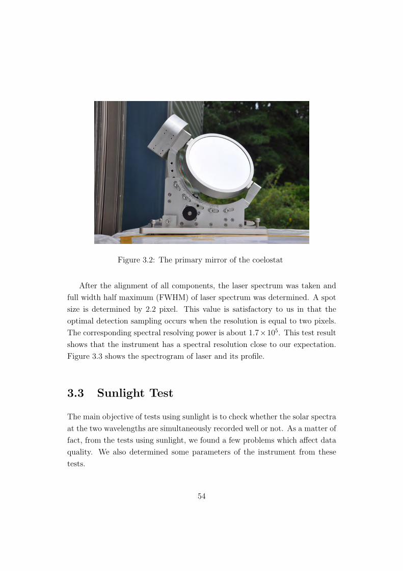
Figure 3.2: The primary mirror of the coelostat
After the alignment of all components, the laser spectrum was taken and
full width half maximum (FWHM) of laser spectrum was determined. A spot
size is determined by 2.2 pixel. This value is satisfactory to us in that the
optimal detection sampling occurs when the resolution is equal to two pixels.
The corresponding spectral resolving power is about 1.7×10⁵. This test result
shows that the instrument has a spectral resolution close to our expectation.
Figure 3.3 shows the spectrogram of laser and its profile.
3.3 Sunlight Test
The main objective of tests using sunlight is to check whether the solar spectra
at the two wavelengths are simultaneously recorded well or not. As a matter of
fact, from the tests using sunlight, we found a few problems which affect data
quality. We also determined some parameters of the instrument from these
tests.
54

Figure 3.3: Enlarged laser spectrogram (upper) and its horizontal profile
(lower). In laser spectrogram, x-direction and y-direction indicate spectral do-
main and spectral domain, respectively. In lower plot, a dashed line presents
gaussian fitting
55
CCD anomaly A pair of spectrograms at Hα and CaII8542 were taken
simultaneously (see right image in Figure 3.6). Contrary to Hα spectrogram,
the CaII spectrogram shows not only solar absorption lines but also a wave-
like pattern. This fringe pattern always appears irrespective of incident angle
of grating or cooling down CCD temperature in CaII8542. After some tests,
we found that this strange pattern is caused by the etaloning effect that are
intrinsic to all back-illuminated CCDs working at NIR and IR wavelengths.
Because back-illuminated CCDs are thin devices (typically 10-20µm) which
become semi-transparent in near infrared, the reflection between the nearly
parallel front and back surface of these devices causes them to act as etalons.
This phenomenon leads to unwanted fringes of constructive and destructive
interference which artificially modulate a spectrum. At IR wavelength where a
silicon is transparent enough that light can traverse the thickness of the CCD
several times, the light to bounce back and forth between the two surfaces.
This interference increases the effective path length in the silicon, but it also
makes a standing wave pattern. At long wavelengths like 700nm above, several
passes cause constructive or destructive interference. Due to slight differences
in the thickness of CCDs from wafer to wafer or chip to chip fabrication, the
fringe patterns are different from CCDs each other. The only way to avoid
the problem is to use front-illuminated CCD hence we replaced DV887 (back-
illuminated) with DV885 (front-illuminated) for CaII8542.
Measurement of grating efficiency During tests, spectrograms at the
same wavelength were recorded at different grating angles, with different in-
tensities. These represent spectrograms of different orders.
The intensity of a spectrogram is the highest when the grating angle is
closest to the blaze angle of the grating. As the grating angle deviates from
the blaze angle, the intensity decreases significantly. The ratio of the intensity
of the brightest spectrogram to the intensity of all the spectrograms represents
grating efficiency. In a limited range of grating angle, we searched all spec-
trograms. After that, the spectral order of each spectrogram was identified.
56
The relative intensity of each spectral order can be calculated using the blaze
function:
I ∝ [sinc(X)]2 = (sinX
X)2, (3.1)
with X defined by
X = πθb
λ(3.2)
= π(sin(α− ϕ) + sin(β − ϕ))b
λ
=mπb
d[cosϕ− sinϕ
tan α+β2
],
where b, d, α, β are the width between adjacent grids, groove density, blaze
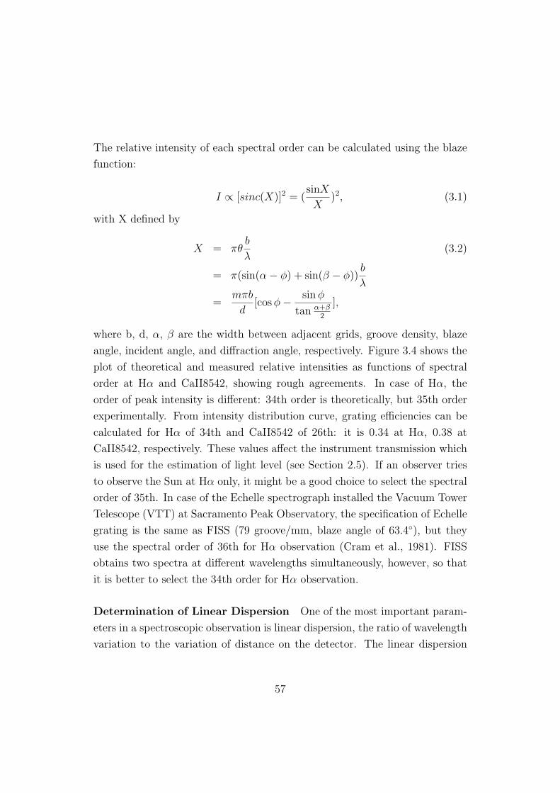
angle, incident angle, and diffraction angle, respectively. Figure 3.4 shows the
plot of theoretical and measured relative intensities as functions of spectral
order at Hα and CaII8542, showing rough agreements. In case of Hα, the
order of peak intensity is different: 34th order is theoretically, but 35th order
experimentally. From intensity distribution curve, grating efficiencies can be
calculated for Hα of 34th and CaII8542 of 26th: it is 0.34 at Hα, 0.38 at
CaII8542, respectively. These values affect the instrument transmission which
is used for the estimation of light level (see Section 2.5). If an observer tries
to observe the Sun at Hα only, it might be a good choice to select the spectral
order of 35th. In case of the Echelle spectrograph installed the Vacuum Tower
Telescope (VTT) at Sacramento Peak Observatory, the specification of Echelle
grating is the same as FISS (79 groove/mm, blaze angle of 63.4), but they
use the spectral order of 36th for Hα observation (Cram et al., 1981). FISS
obtains two spectra at different wavelengths simultaneously, however, so that
it is better to select the 34th order for Hα observation.
Determination of Linear Dispersion One of the most important param-
eters in a spectroscopic observation is linear dispersion, the ratio of wavelength
variation to the variation of distance on the detector. The linear dispersion
57
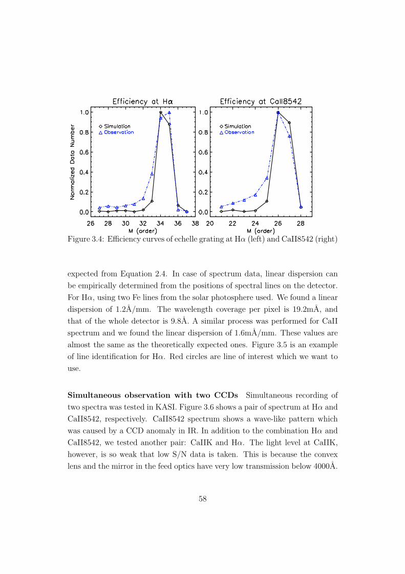
Figure 3.4: Efficiency curves of echelle grating at Hα (left) and CaII8542 (right)
expected from Equation 2.4. In case of spectrum data, linear dispersion can
be empirically determined from the positions of spectral lines on the detector.
For Hα, using two Fe lines from the solar photosphere used. We found a linear
dispersion of 1.2A/mm. The wavelength coverage per pixel is 19.2mA, and
that of the whole detector is 9.8A. A similar process was performed for CaII
spectrum and we found the linear dispersion of 1.6mA/mm. These values are
almost the same as the theoretically expected ones. Figure 3.5 is an example
of line identification for Hα. Red circles are line of interest which we want to
use.
Simultaneous observation with two CCDs Simultaneous recording of
two spectra was tested in KASI. Figure 3.6 shows a pair of spectrum at Hα and
CaII8542, respectively. CaII8542 spectrum shows a wave-like pattern which
was caused by a CCD anomaly in IR. In addition to the combination Hα and
CaII8542, we tested another pair: CaIIK and Hα. The light level at CaIIK,
however, is so weak that low S/N data is taken. This is because the convex
lens and the mirror in the feed optics have very low transmission below 4000A.
58
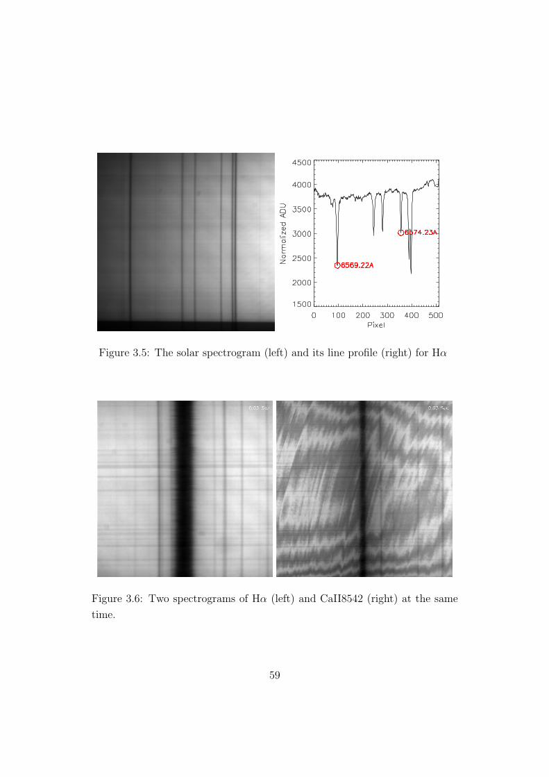
Figure 3.5: The solar spectrogram (left) and its line profile (right) for Hα
Figure 3.6: Two spectrograms of Hα (left) and CaII8542 (right) at the same
time.
59

Interlocking between CCD and scanner Synchronization between the
CCD and the scanner was tested in KASI and BBSO. The test of interlocking
between a CCD and the scanner was performed by using resolution panel
located at pupil in AO. If the interlocking works well, we can see a well-
constructed raster image of resolution panel illuminated by sunlight. Figure 3.7
shows such a raster scan image for the resolution panel taken at Hα center.
Resolution patterns are well constructed. During the observation, there was
air disturbance. On the right side of image, distortion in vertical direction
appears. This fluctuation is caused by airplane on the sky at that time. We
conclude that the scanner and a CCD are working so well.
Figure 3.8 shows raster scan images constructed at Hα and CaII8542 at
KASI on Dec 14, 2009. Exposure time, slit width, step size per scan, frame,
scanning time, and FOV are 30 ms, 16 µm, 16 µm, 512 frames, 50 sec, and
1500′′×1500′′, respectively. We can identify several features in raster images
such as faint prominence on limb, active regions, plages, and filaments. In
the CaII image displays horizontal lines the CCD anomaly. From these raster
images, we conclude that two CCDs and scanner are organized well enough.
More interlocking tests by using FISS will be given in the next Chapter.
Light level and spatial resolution A main discrepancy between the esti-
mation by the design and the determination from observation is in the light
level; the level of light detected by CCDs is too low. Moreover, current AO
is not working well enough to achieve the diffraction-limited resolution. To
increase the light level, we increased the slit width from 16µm to 32µm. This
means that an amount of light increases twice. Secondly, 1×2 binning was
applied to CCD A, and 2×4 binning to CCD B, which results in the effective
pixel size of 0.16′′ in the slit direction. Due to the current limitation of AO
capability, it is good enough to observe the Sun for a while. If the performance
of AO is improved so that it can achieve the diffraction-limited resolution, the
binning can be reset to the default values. Thanks to the combined effect of a
wider slit and the binning, the light level is four times the original. Observing
60

Figure 3.7: Raster scan image of the resolution panel on May 10, 2010. On
right side (square), the distortion appears in vertical direction because of the
fluctuation caused by an airplane.
61

Figu
re3.8:
Raster
scanim
agesof
theSuncon
structed
atHα(left)
andCaII8542
(right)
onDecem
ber
14,
2009.Horizon
tallin
eson
CaII8542
image
arecau
sedbytheCCD
anom
alyat
IR.
62

Table 3.1: Typical observing parameters
parameters CCD A CCD B
wavelength Hα 6562.8A CaII 8542A
slit width 32 µm (0.16′′) 32 µm (0.16′′)
binning 1 × 2 2 × 4
integration times 30ms 30-90ms
scan step size 32µm (0.16′′) 32µm (0.16′′)
scan frames 100 - 400 100 - 400
field of view (16 - 64′′) × 40′′ (16 - 64′′) × 40′′
observing duration 0.5 - 1 h 0.5 - 1 h
CCD cooling temperature −50 C −50 C
FOV of flat fielding 64′′× 40′′ 64′′× 40′′
parameters are depicted in Table 3.1.
3.4 Conclusion
After installing of all optics and moving components on a vertical table, various
tests were mainly performed at KASI. A detailed position of each component
was decided by laser test, and the pixel resolution was obtained. The test
by sunlight using coelostat enables us to find unexpected problems and to
measure spectrograph parameters of each component. Through light test, we
had opportunity to improve the FISS performance. We confirmed that scanner
and CCDs operate well.
63

64

Chapter 4
Early Observations
4.1 Data processing
Raw data obtained with FISS are saved in files of FITs format. There are
three kinds of data – science, bias/dark, and flat/calibration data. Basic data
processing has been performed using IDL procedures and functions. Here we
describe the process.
Bias/dark, flat correction The method to take bias/dark, flat/calibration
file are already mentioned in Chapter 2. Science data and bias/dark data
have the same bias values. Moreover, exposure time of science data is the
same as that of bias/dark data. Flat/calibration data contain seven spectro-
grams taken at different grating angles. Each spectrogram comes out of the
averaging of about 400 frames. It is necessary to separate slit pattern and non-
slit pattern. Slit pattern is inferred from the average of all the spectrograms
over the spectral direction. We divide seven average spectrograms by this slit
pattern, and determine the non-slit pattern from them using the flat fielding
method suggested by Chae (2004). Subtracting bias/dark data from science
data and dividing them by the product of the slit pattern and the non-slit pat-
tern completes basic data processing. Figure 4.1 presents examples of frames
65
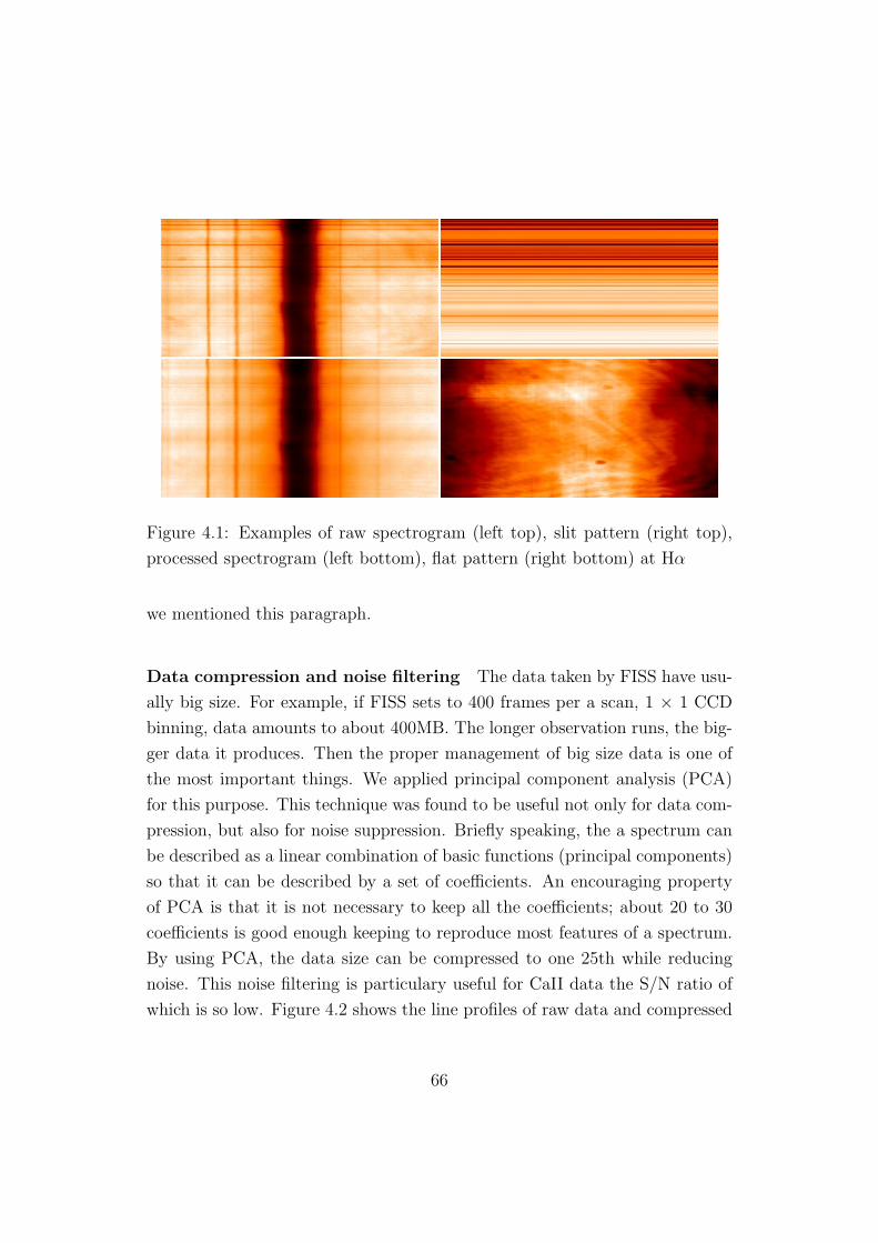
Figure 4.1: Examples of raw spectrogram (left top), slit pattern (right top),
processed spectrogram (left bottom), flat pattern (right bottom) at Hα
we mentioned this paragraph.
Data compression and noise filtering The data taken by FISS have usu-
ally big size. For example, if FISS sets to 400 frames per a scan, 1 × 1 CCD
binning, data amounts to about 400MB. The longer observation runs, the big-
ger data it produces. Then the proper management of big size data is one of
the most important things. We applied principal component analysis (PCA)
for this purpose. This technique was found to be useful not only for data com-
pression, but also for noise suppression. Briefly speaking, the a spectrum can
be described as a linear combination of basic functions (principal components)
so that it can be described by a set of coefficients. An encouraging property
of PCA is that it is not necessary to keep all the coefficients; about 20 to 30
coefficients is good enough keeping to reproduce most features of a spectrum.
By using PCA, the data size can be compressed to one 25th while reducing
noise. This noise filtering is particulary useful for CaII data the S/N ratio of
which is so low. Figure 4.2 shows the line profiles of raw data and compressed
66
data. Compressed data match raw data well except for noise.
Wavelength calibration There are lots of absorption lines near the wave-
lengths of our interest: Hα and CaII8542. Absorption lines come from either
the Sun or the Earth. If a violent activity of the Sun happens, solar absorption
lines may be modified or their positions may be shifted. Even photospheric
lines might be affected a little. Hence wavelength calibration against solar
lines is not suitable. On the other hand, telluric lines from atmosphere of the
Earth provide a good reference for wavelength calibration because atmospheric
line is not affected by the Sun. By comparing spectral lines, the FISS spectra
with the reference spectrum from atlas, we identified solar and telluric lines.
Using the identified terrestrial lines, we determine not only linear dispersion
of the spectrograph, but also the wavelengths solar lines. The values of linear
dispersion per pixel and line position (Hα, CaII8542) in pixel are recorded in
FITs header.
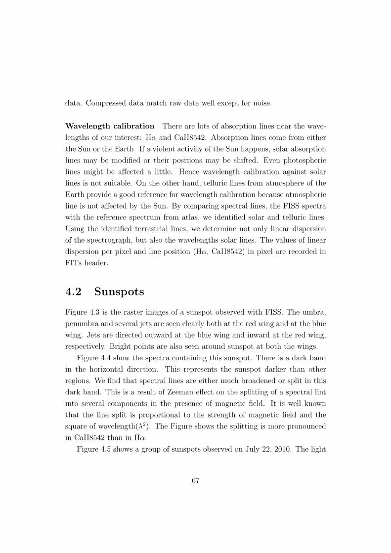
4.2 Sunspots
Figure 4.3 is the raster images of a sunspot observed with FISS. The umbra,
penumbra and several jets are seen clearly both at the red wing and at the blue
wing. Jets are directed outward at the blue wing and inward at the red wing,
respectively. Bright points are also seen around sunspot at both the wings.
Figure 4.4 show the spectra containing this sunspot. There is a dark band
in the horizontal direction. This represents the sunspot darker than other
regions. We find that spectral lines are either much broadened or split in this
dark band. This is a result of Zeeman effect on the splitting of a spectral lint
into several components in the presence of magnetic field. It is well known
that the line split is proportional to the strength of magnetic field and the
square of wavelength(λ2). The Figure shows the splitting is more pronounced
in CaII8542 than in Hα.
Figure 4.5 shows a group of sunspots observed on July 22, 2010. The light
67

Figure 4.2: The comparison of raw data profiles with compressed data pro-
files. In upper row, solid lines and red dashed lines represent raw data profiles
and compressed data profiles at Hα and CaII8542, respectively. Differences
between raw data profiles and compressed data profiles are seen in lower row
68

bridge is visible inside the major sunspot. During this observation, the AO
was operating and short-exposure TiO images of the same region were taken
simultaneously. This is the first coordinated observation of FISS and other
instruments. A speckle-reconstructed TiO image of the region is shown in
Figure 4.6.
4.3 Filaments
There are two kinds of filaments; quiescent filaments and active region fila-
ments. Quiescent filaments are stabler and bigger than active filaments. We
observed both kinds of filaments using FISS. Figure 4.7 shows a portion of a
quiescent filament. It shows both the spine and barb structure. The barbs
protrude from the side of the filament. Figure 4.8 shows another quiescent
filament. This filament appears to be patchy rather than elongated, which is
unusual. Figure 4.9 is a portion of another filament. A few dark threads are
seen along the body of this filament. Figure 4.10 is an example of an active
region filament. Generally it is well known that active region filament are more
dynamic, short lived than quiescent filament.
4.4 Active Regions
Figure 4.11 presents raster images of an active region in the emerging phase.
An arch filament system appears in line center images. It is a characteristic
feature of a developing active region on the Sun that connects areas of opposite
magnetic polarity. Individual arches have lengths of about 30,000km, height of
arches of 4,000-15,000km and lifetime of each filament of 30 minutes (Bruzek,
1967). Many bright points, called ellerman bombs, are visible at the red and
the blue wing images. The lifetime are less than 10 minutes. Generally its
spectrum is characterized by very broad emission wings at Hα.
69
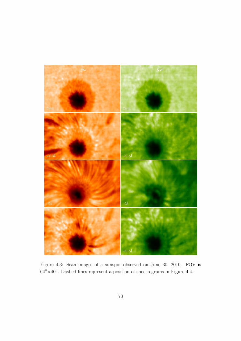
Figure 4.3: Scan images of a sunspot observed on June 30, 2010. FOV is
64′′×40′′. Dashed lines represent a position of spectrograms in Figure 4.4.
70
Figure 4.4: Sunspot spectrograms of Hα and CaII8542.
71

Figure 4.5: Sunspot images on July 22, 2010. FOV is 40′′×40′′.
72

Figure 4.6: Speckle reconstruction image of sunspot group (AR 11089) at TiO
band (706nm) on July 22, 2010.
73

Figure 4.7: Scan images of quiescent filament on July 29, 2010. FOV is
56′′×40′′.
74
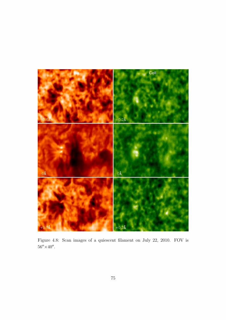
Figure 4.8: Scan images of a quiescent filament on July 22, 2010. FOV is
56′′×40′′.
75

Figure 4.9: Scan images of a quiescent filament on July 16, 2010. FOV is
64′′×40′′.
76

Figure 4.10: Scan images of an active region filament on June 25, 2010. FOV
is 72′′×40′′.
77
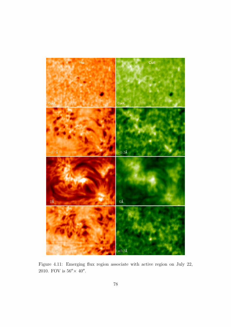
Figure 4.11: Emerging flux region associate with active region on July 22,
2010. FOV is 56′′× 40′′.
78

4.5 Quiet Regions
Figure 4.12 is a quiet region near the center of the solar disk. Dark patches and
bright points appear in FOV. Although this quiet region has no conspicuous
feature, dynamical features always occur in small scale.
4.6 Prominence
A Prominence is quite different from its disk counterpart, a filament. Con-
trary to filaments, spectral lines from a prominence on solar limb appear in
emission. When a prominence is the observing target, it is hard to operate
AO simultaneously because there is no good reference for AO in the limb. The
image motion cannot be corrected for by the AO, and as a result we obtain
raster scan images that are no so regular in the slit direction. Figure 4.13 is
the prominence spectra from limb inside to limb outside.
4.7 Conclusion
After testing, many kinds of imaging spectroscopy data are obtained by
FISS. We have observed various chromospheric features such as active regions,
sunspots, filaments, and so on. The data taken by FISS are quite good for
studying the dynamical characteristics of the chromosphere. Through these
observations of the Sun using FISS, we have acquired many ideas for better
observing the Sun and improving FISS capability. We plan to reflect these
ideas to FISS as soon as possible. We believe that the data obtained by the
spectrograph will help us to discover the dynamics and physical conditions of
the Sun.
79

Figure 4.12: Scan images of quiet region near disk center of the Sun on June
25, 2010. FOV is 64′′×40′′.
80

Figure 4.13: Hα (upper row) and CaII (lower row) spectrograms taken at the
solar limb and a prominence outside it.
81

82
Chapter 5
Determination of physical
parameters of prominences
5.1 Introduction
A prominence, meaning protuberance in French, is one of most notable features
seen on solar limb above at chromosphere. Prominences are classified into two
types according to their morphology: quiescent and active prominences. Qui-
escent prominences are stabler than active prominences, and usually maintain
their shapes for a long time. Their shapes are like hedgerow, curtain, arch, etc.
They are of 60 - 600Mm length, 10 - 100Mm height, 4 - 15Mm width (Priest,
1989). Quiescent prominences are located above polarity inversion lines and
consist of many fine threads. Active prominences often occur near active re-
gions and are associated with solar flares and other violent events. They have
stronger magnetic field and higher temperature than quiescent prominences.
Also their shapes last for more or less short durations. Surges, sprays, post-
flare loops are examples of active prominences. Although quiescent promineces
are globally stable, they exhibit rapid variation in their fine structure within
a few minutes from ground-based and space-based observation.
It has been frequently attempted to determine their physical quantities.
83
Temperature is one of the most important parameters. Ellison (1952) tracked
the same prominence on the limb and on the disk, and obtained a kinetic
temperature of 10,000 - 20,000 K. Jefferies & Orrall (1961) obtained a mean
kinetic temperature of about 12,000 K based on Blamer and Paschen jump for
quiescent prominences. Furthermore by using line width between the higher
Balmer and metallic lines, they obtained the temperature of less than 8,000 K
(Jefferies & Orrall, 1962). They concluded that this discrepancy is caused by
temperature and density gradients inside the matter of quiescent prominences.
On the other hand, Hirayama (1963) measured temperature of 4,500 - 8,500 K
using hydrogen lines and metallic lines.
Nikolsky et al. (1971) obtained T=10,000 K, ξ=6km/s using analysis of
stark effect on Balmer lines (up to number 36) from quiescent prominence. Hi-
rayama (1971) found that the prominence has temperature and non-thermal
velocity gradient from central region to periphery. In central region, tempera-
ture is 6,000 - 7,000 K and at the outer region, it is about 12,000 K. Zhang et
al. (1987) obtained T=7,500 K by applying least square method. Stellmacher
et al. (2003) obtained T=8,000 - 9,000 K, ξ=3 - 8km/s from CaII8542 and
HeI10830 observation.
Many authors measured temperature of prominences , but the determined
temperatures are somewhat different (Kawaguchi, 1966; Kubota, 1968; Mo-
rozhenko, 1974; Mouradian & Leroy, 1977; Landman et al., 1977; Mein et al.,
1991; Kejun et al., 1998). The common method to determine the temperature
is to measure the width of optically thin lines and to compare with each other.
Note that line width contains not only the effect of temperature but also that
of non-thermal velocity. If it is possible to separate between the two compo-
nents well, we will be able to better estimate the prominence temperature.
Our new instrument, FISS, has a capability to simultaneously take two
spectra of two different lines — Hα line and CaII line at 8542 A— with high
spectral resolution and with high spatial resolution. Then we expect that
temperature can be determined from the widths of these lines more precisely
than previous researches.
84
In this Chapter, we estimate physical parameters at specific positions of
two prominences by using a simple model.
5.2 Model of Radiative Transfer
As we know well, radiative transfer equation is described by
I = I0e−τ +
∫ τ
0Se−tdt, (5.1)
where τ and S are optical thickness and source function, respectively. If there
is no background radiation, source function is constant along the line of sight,
Equation 5.1 may be simply rewritten as
I = S(1− e−τ ) . (5.2)
Since collisional broadening is negligible in prominences, only Doppler broad-
ening needs to be considered. Thus optical thickness has a Gaussian profile
τ = τ0 exp(λ− λc
∆λD
)2, (5.3)
where ∆λD is Doppler width and λC is the position of line center.
In the solar atmosphere, individual atoms move in random directions con-
tinuously with the average speed so it is proportional to the square root of
ion/atom temperature. These random motions of ions/atmos result in line
broadening called thermal Doppler broadening. The Doppler width of thermal
broadening is given by
∆λD =λ
c
√2kT
M, (5.4)
where λ is the wavelength at rest, T is ion temperature, M is the mass of ion.
In reality, line widths determined from observations are broader than ther-
mal broadening. This is why it is believed that there are unresolved motion,
called non-thermal motion. With non-thermal motion taken into account, the
85
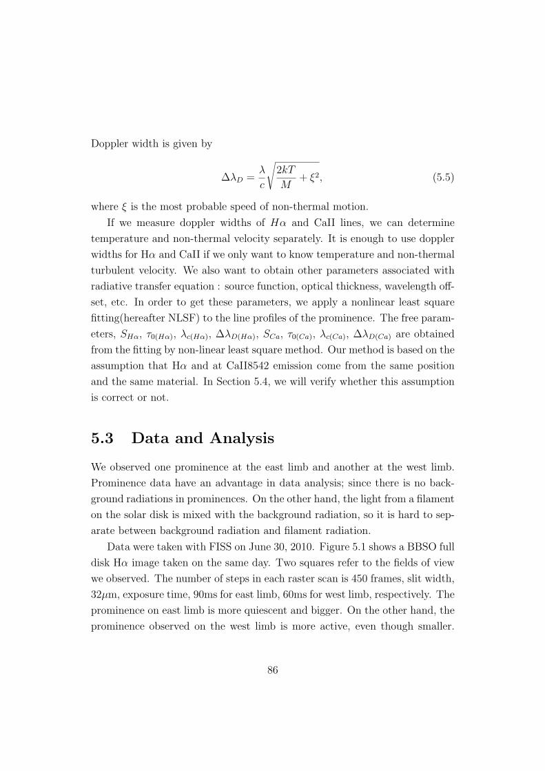
Doppler width is given by
∆λD =λ
c
√2kT
M+ ξ2, (5.5)
where ξ is the most probable speed of non-thermal motion.
If we measure doppler widths of Hα and CaII lines, we can determine
temperature and non-thermal velocity separately. It is enough to use doppler
widths for Hα and CaII if we only want to know temperature and non-thermal
turbulent velocity. We also want to obtain other parameters associated with
radiative transfer equation : source function, optical thickness, wavelength off-
set, etc. In order to get these parameters, we apply a nonlinear least square
fitting(hereafter NLSF) to the line profiles of the prominence. The free param-
eters, SHα, τ0(Hα), λc(Hα), ∆λD(Hα), SCa, τ0(Ca), λc(Ca), ∆λD(Ca) are obtained
from the fitting by non-linear least square method. Our method is based on the
assumption that Hα and at CaII8542 emission come from the same position
and the same material. In Section 5.4, we will verify whether this assumption
is correct or not.
5.3 Data and Analysis
We observed one prominence at the east limb and another at the west limb.
Prominence data have an advantage in data analysis; since there is no back-
ground radiations in prominences. On the other hand, the light from a filament
on the solar disk is mixed with the background radiation, so it is hard to sep-
arate between background radiation and filament radiation.
Data were taken with FISS on June 30, 2010. Figure 5.1 shows a BBSO full
disk Hα image taken on the same day. Two squares refer to the fields of view
we observed. The number of steps in each raster scan is 450 frames, slit width,
32µm, exposure time, 90ms for east limb, 60ms for west limb, respectively. The
prominence on east limb is more quiescent and bigger. On the other hand, the
prominence observed on the west limb is more active, even though smaller.
86

Since AO was not working well, an irregularity appeared in raster scan images
across the slit direction. After selecting a few positions in the raster scan
images, we analyzed Hα and CaII8542 data.
Position alignment FISS uses two CCDs with different chip sizes. Further-
more, the specific FOV of each CCD is subject to optical alignment. Due to
the difference in chip size and alignment, the two CCD come to have different
FOVs along the slit direction. Then the co-alignment between two spectral
data is essential for data analysis. The relative offset along the slit direc-
tion was found to be 7 pixels. This offset value may change whenever optical
configuration changes.
Aureole correction If optical configuration is ideal, there should be no
light above prominences in our measurements. In reality, however, stray light
is identified on the slit surface. Stray light enters the spectrograph and ap-
pears as a ghost spectrogram on CCD. Although this aureole is fainter than
the prominences, it still affects the line profiles of prominences seriously. If
prominence intensity is low, we cannot measure line width because of the con-
tamination by the aureole. In order to remove stray light, we used a portion
of spectrum at the location outside prominences. The selected spectrum is
averaged along slit direction. This averaged spectrum is subtracted from each
row of the spectrograms, which is like bias/dark correction. Figure 5.3 shows
a raw spectrogram and the processed spectrogram with stray light taken out.
5.4 Results
As the first step, we arbitrarily selected two positions on the east limb promi-
nence (see Figure 5.4), an applied the NLSF to the spectra at those points.
Fitting result 1 Firstly we determined a few parameters from line profiles
of Hα and CaII8542 : source function (S), optical thickness (τ0), wavelength
87

Figure 5.1: Hα full disk image on June 30, 2010 in BBSO. Two squares repre-
sent field of view of FISS.
88

Figure 5.2: Scan images at Hα, CaII in east (left column) and west limb
prominence (right column)
Figure 5.3: A raw spectrogram (upper) and a correction spectrum subtracted
aureole light (lower) at Hα.
89

Figure 5.4: Two points at the east prominence of Hα (upper) and CaII8542
(lower)
offset (λC) and line width (∆λD) using NLSF. From the obtained line widths
(∆λD(Hα),∆λD(Ca)), we infer the temperature and non-thermal velocity.
Figure 5.5 presents line profiles in comparison with fittings for positions A
and B, respectively. The Hα line profile of position A displays central reversal.
Stellmacher et al. (2003) found that central reversal occurs in Hα emission line
when optical thickness is greater than 4. This indicates that source function
is not constant over the optical path, and self absorption exists in an optically
thick layer. In spite of central reversal in position A, the fit appears fairly
good not only in the wing but also in the central region. The CaII8542 profile
is fit better. In comparison with Hα, the optical thickness of the CaII line is
quite small.
Reliability of optical thickness From fitting of Hα data, we found that
optical thickness is mostly greater than 1. As mentioned before, if prominence
material is optically thin, the line profile is approximated to be gaussian. Based
on the optical thickness obtained from fitting, this optically thin approximation
90

Figure 5.5: Fitting results of Hα and CaII8542 on position A (upper row) and
B (lower row). Left column represents Hα profiles and fittings, while right
column shows CaII8542 profiles and fittings.
91
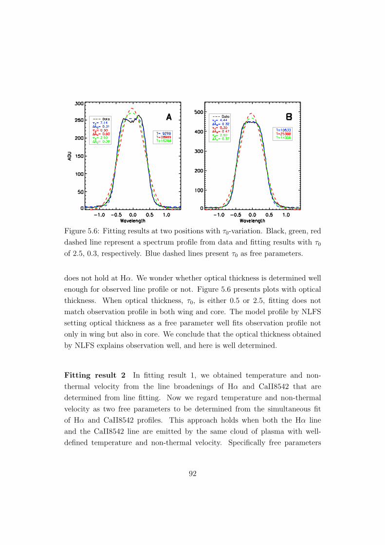
Figure 5.6: Fitting results at two positions with τ0-variation. Black, green, red
dashed line represent a spectrum profile from data and fitting results with τ0
of 2.5, 0.3, respectively. Blue dashed lines present τ0 as free parameters.
does not hold at Hα. We wonder whether optical thickness is determined well
enough for observed line profile or not. Figure 5.6 presents plots with optical
thickness. When optical thickness, τ0, is either 0.5 or 2.5, fitting does not
match observation profile in both wing and core. The model profile by NLFS
setting optical thickness as a free parameter well fits observation profile not
only in wing but also in core. We conclude that the optical thickness obtained
by NLFS explains observation well, and here is well determined.
Fitting result 2 In fitting result 1, we obtained temperature and non-
thermal velocity from the line broadenings of Hα and CaII8542 that are
determined from line fitting. Now we regard temperature and non-thermal
velocity as two free parameters to be determined from the simultaneous fit
of Hα and CaII8542 profiles. This approach holds when both the Hα line
and the CaII8542 line are emitted by the same cloud of plasma with well-
defined temperature and non-thermal velocity. Specifically free parameters
92
are SHα, τ0(Hα), λC(Hα), T, ξ, SCa, τ0(Ca), and λC(Ca). Figure 5.7 shows the re-
sults for fitting. Line profiles are well fit by models. If the two lines are
emitted by different clouds of plasma with different temperature or different
non-thermal motion, fitting may not be good enough. We confirm from the fit-
ting that the temperature and non-thermal velocity seen at Hα and CaII8542
are the same.
Fitting result 3 All of results which we showed above are based on the as-
sumption that the light from the Sun at Hα and CaII8542 must come from the
same position and the same material. Is this assumption really true? If this is
true, we expect that line of sight velocity at specific position should have the
same value in both Hα and CaII8542 line. In radiative transfer equation, opti-
cal thickness profile depends on wavelength offset (see Equation 5.3) that is a
direct measure of line of sight velocity. We tried to obtain several free param-
eters including temperature, non-thermal velocity, and line of sight velocity
using NLSF through the simultaneous fit of Hα and CaII8542 profiles. Free
parameters are SHα, τ0(Hα), Vlos, T, ξ, SCa, and τ0(Ca), respectively. Results are
depicted in Figure 5.8. Models well match observed profiles at each position.
We conclude that the light seen at Hα and CaII8542 come from same position
and material.
Temperature variation with height After taking physical parameters at
2 points, we investigated the variation of temperature and non-thermal ve-
locity with height. In Figure 5.9, a group of symbols with the same shape
represents a sample. Four samples are investigated to study the variation of
temperature and non-thermal velocity with height. This is a tendency of tem-
perature increase with height (see Figure 5.10). It is well known that both
temperature and non-thermal velocity increase from prominence center to its
periphery (Hirayama, 1971). He found the temperature varies from 6,000 -
7,000K at the center, 12,000K at the boundary. In our results, however, tem-
peratures are relatively high. The distribution of non-thermal velocity are not
93

Figure 5.7: Fitting results in Hα and CaII8542 at both the position A (upper)
and the position B (lower).
94
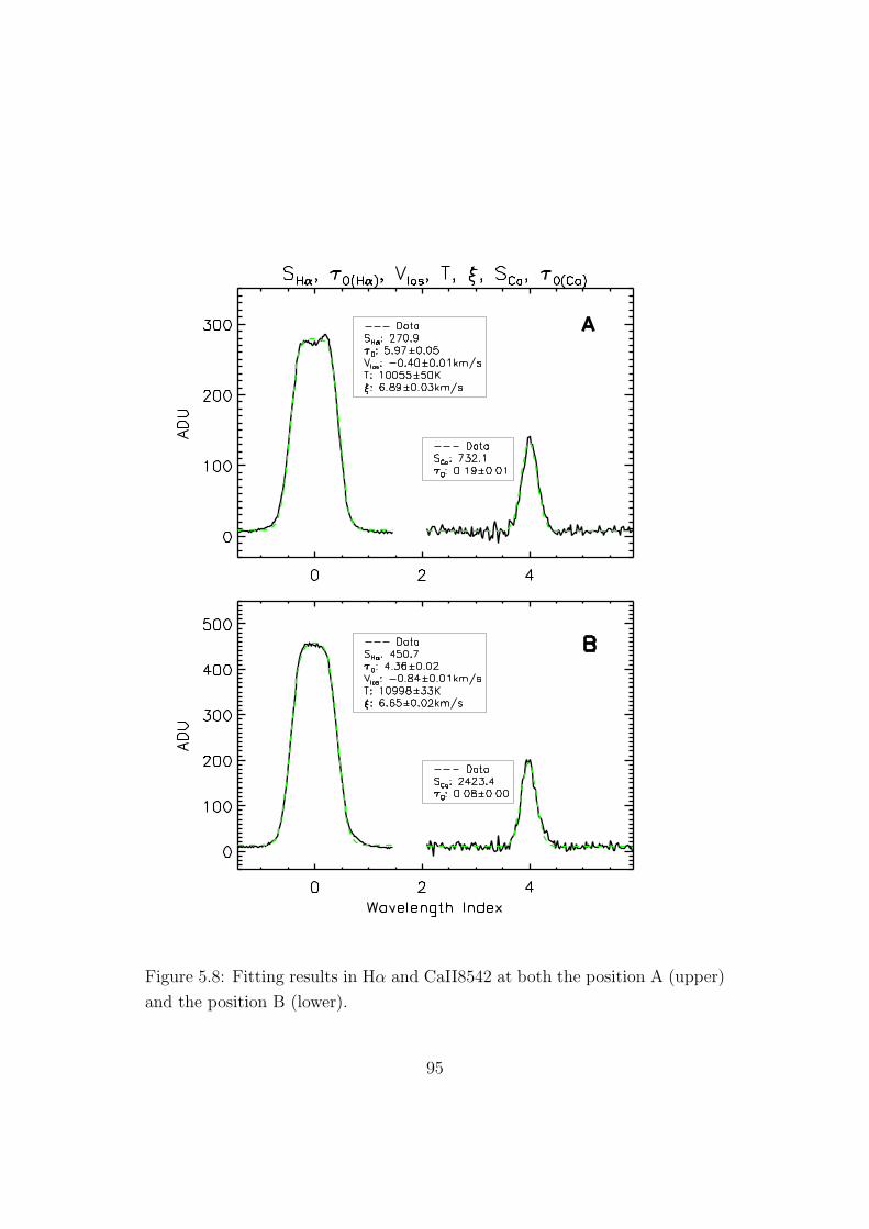
Figure 5.8: Fitting results in Hα and CaII8542 at both the position A (upper)
and the position B (lower).
95

Figure 5.9: Positions of interest with height in the east prominence.
found in our results.
Temperature – non-thermal velocity distribution In order to know the
range of temperature and non-thermal turbulent velocity, many positions are
selected in east and west prominence. Figure 5.11 is the raster scan image in
east limb prominence with positions of interest being marked. There are two
kinds of plots, line width - line width plots and temperature versus non-thermal
velocity plots (see Figure 5.12). Since the doppler width contains temperature
and non-thermal velocity, isothermal curve and iso-nonthermal velocity curve
can be plotted in the line width - line width plot. Blue lines (diagonal lines)
represent iso-temperature curves and red lines (horizontal lines) indicate iso-
nonthermal velocity curve. In this plot, we found that Hα line broadening is
more sensitive to temperature than non-thermal velocity, while CaII8542 line
broadening is sensitive to non-thermal velocity. That is, Hα line broadening
mostly reflects thermal broadening, while CaII8542 line broadening does non-
96

Figure 5.10: Temperature variations with height.
thermal broadening. Spot symbols represent the values obtained by NLSF.
Based on the iso-temperature curve and iso-nonthermal velocity curve, we
found that the ranges of temperature and non-thermal velocity are 7,500 -
13,000 K and 5 - 11km/s, respectively. In the temperature - non-thermal
velocity plot, an error bar is shown for each spot. The scale of error bar is too
small to be seen in the line width - line width plot.
The same analysis was performed in the west prominence as well (see Fig-
ure 5.13). Figure 5.14 shows the two plots. These plots show the same char-
acteristics as the plots of the east limb prominence. Since light level is so low,
it’s hard to identify profiles of CaII8542 line. Furthermore, AO was not work-
ing well, so the seeing has not been compensated for effect. These conditions
cause CaII line to have low S/N ratios. In the west limb prominence, there is
no tendency for temperature with height.
97

Figure 5.11: Sampling positions of Hα (upper) and CaII (lower) in the east
prominence.
Figure 5.12: Doppler width (∆λD(Hα),∆λD(Ca)), temperature, and non-
thermal velocity plot (left) and temperature – non-thermal velocity plot (right)
in the east prominence.
98

Figure 5.13: Sampling positions in the west prominence.
Figure 5.14: Doppler width (∆λD(Hα),∆λD(Ca)), temperature, and non-
thermal velocity plot (left) and temperature – non-thermal velocity plot (right)
in the west prominence.
99

Figure 5.15: The position where the line broadening is biggest at Hα (upper)
and CaII8542 (lower).
Determination of maximum temperature We tried to determine maxi-
mum temperature of prominence. As we mentioned above, Hα profile is more
sensitive to temperature than to non-thermal velocity. Then we tried to search
the position where line width is biggest (see Figure 5.15). The position is at
the outer boundary of the prominence that is very faint. At this position, there
is no light of CaII8542. Then determined line broadening was 0.43A. The cor-
responding temperature range is 16,000 - 22,000 K under the assumption of
non-thermal velocity of 4 - 11km/s. If non-thermal velocity is about 7km/s
which is average speed of our result, maximum temperature of prominence we
analyzed is about 20,000 K. This result is consistent with previous research
(Hirayama, 1985) which was inferred from emission-line wings.
100

5.5 Conclusion
We analyzed prominences taken on the east and west limb using non-linear
least square method for radiative transfer. Physical parameters obtained by
data analysis are checked to see whether they are reliable or not. We found
that Hα optical thickness is greater than 1 in the prominences. We identified
that our analysis method can fit observation profile well. Temperature range,
non-thermal velocity, maximum temperature of prominence obtained from our
analysis are 7,500 - 13,000 K, 5 - 11km/s, and 20,000 K, respectively. We also
confirmed that temperature increases with the height inside each prominence.
Through the data analysis, we found that the same temperature, non-thermal
velocity, line of sight account for Hα and CaII spectral profiles as we assumed.
This result supports that the light seen Hα and CaII8542 comes from the same
position and the same material.
101

102

Chapter 6
Conclusion
I participated in the development of a new instrument to observe the Sun, Fast
Imaging Solar Spectrograph (FISS). Now FISS is installed in the Coude room
at Big Bear Solar Observatory performing solar observations successfully.
The 1.6 meter New Solar Telescope (NST), the biggest telescope, has been
built at Big Bear Solar Observatory (BBSO). To study fine structure and its
dynamics of solar chromosphere by using NST, we proposed the spectrograph
with high spectral resolution, high time resolution and doing imaging spec-
troscopy. Spectrograph concept was decided and optical design was performed.
At the same time, FISS throughput was calculated. The distinctive charac-
teristics of FISS are dual band, Littrow mounting, Echelle grating, imaging
using the field scanner. Each component of FISS was designed, made, inte-
grated in Korea Astronomy and Space Science Institute (KASI). In addition,
the control program was developed. After integration in hardware and in soft-
ware, we tested our spectrograph and measured the performance of FISS.
Through tests, we concluded that the performance of spectrograph is close to
our requirements. After completing tests in Korea, FISS was moved to BBSO
and was installed on the vertical table on the Coude room. We observed
chromospheric features several times with FISS. During observations, the pro-
grams for image processing and data compression were developed. The data
103

obtained by the instrument show various characteristics of the solar chro-
mosphere. Furthermore, we obtained many ideas for the improvement of our
system for better observation.
By analyzing prominence data obtained by FISS, we determined physical
parameters such as temperature, non-thermal velocity, optical thickness and
so on. We confirmed that our non-linear model of radiative transfer explains
well not only spectral profiles of optically thin regions but also those of op-
tically thick regions in prominences. Furthermore, we conclude that at least
at regions we analyzed the lights at Hα and CaII8542 come from the same
position and the same material. The ranges of temperature and non-thermal
turbulent velocity are 7,500 - 13,000 K, 5 - 11km/s, respectively. The maxi-
mum temperature of prominences is measured to be about 20,000 K, which
is consistent with previous report by Hirayama (1985).
104

Bibliography
Ahn, K., Chae, J., Park, H.-M., Nah, J., Park, Y.-D., Jang, B.-H., Moon, Y.-J.,
2008, JKAS, 41, 39
Ahn, K., 2009, Ph.D. Thesis, Seoul National University
ANDOR, 2009, Document, User’s Guide to : ANDOR SDK
Bruzek, A., 1967, SoPh, 2, 451
Cauzzi, G., Reardon, K. P., Uitenbroek, H., Cavallini, F., Falchi, A., Falciani, R.,
Janssen, K., Rimmele, T., Vecchio, A., Woger, F., A&A, 480, 515
Chae, J., 2004, SoPh, 221, 1
Cram, L. E., Robinson, R. D, Mauter, H. A., Mann, G. R., and Phillis, G. L., 1981,
SoPh, 71, 237
DELTA TAU, 2003, Document, Software Reference Manual : PCOMM32PRO
Dere, K. P., Bartoe, J. -D. F., Brueckner, G. E., 1986, ApJ, 305, 947
Ding, M. D., Fang, C., and Huang, Y. R., 1995, SoPh, 158, 81
Ellison, M. A., 1952, MNRAS, 112, 679F
HEASARC, 2009, Document, CFITSIO User’s Reference Guide - An Interface to
FITS Format Files for C Programmers
105

Hirayama, T., 1963, PASJ, 15, 122
Hirayama, T., 1971, SoPh, 17, 50
Hirayama, T., 1985, Soph, 100, 415
Jefferies, J. T. & Orrall, F., Q., 1961, ApJ, 134, 747
Jefferies, J. T. & Orrall, F., Q., 1962, ApJ, 135, 109
Kawaguchi, I., 1966, PASJ, 18, 362
Kejun, L., Schmieder, B., Malherbe, J. -M., Roudier, TH., Wiik, J. -E., 1998, SoPh,
183, 323
Kubota, J., 1968, PASJ, 20, 317
Landman, D. A., Edberg, S. J., Laney, C. D., 1977, ApJ, 218, 888
Landman, D. A., & Mongillo, M., 1979, ApJ, 230, 581
Mein, P., 1977, SoPh, 54, 45
Mein, P. & Mein, N., 1991, SoPh, 136, 317
Mein, P. and Malherbe, J. -M., Heinzel, P., Kneer, F., Uexkull, V. M., Staiger, J.,
1997, SoPh, 172, 161
Morozhenko, N. N., 1974, SoPh, 34, 303
Mouradian, J., Leroy, J. L., 1977, SoPh, 51, 103
Nah, J., Chang, B. -H., Park, Y. -D., Choi, S., Kim, K. D., Lim, I. S., Chae, J.,
Ahn, K., Park, H. -M., 2009, Technical Report in KASI, 33
Nikolsky, G. M., Gulyaev, R. A., Nikolskaya, K. I., 1971, SoPh, 21, 332
PARKER AUTOMATION, 1998, Document, 6K Series Programmer’s Guide
106

Penn, M. J., Mickey D. L., Canfield, R. C., and Labonte, B. J., 1991, SoPh, 135,
163
Priest, E. R., 1989, in Dynamics and Structure of Quiescent Solar Prominences
(Dordrecht : Kluwer), 1
Stellmacher, G., 1969, A&A, 1, 62
Stellmacher, G. & Wiehr, E., 1994, A&A, 290, 655
Stellmacher, G., Wiehr, E., Dammasch, I. E., 2003, SoPh, 217, 133
Stellmacher, G. & Wiehr, E., 2005, A&A, 431, 1069
Stellmacher, G. & Wiehr, E., 2008, A&A, 489, 773
Zhang, Q. Z., Livingston, W. C., Hu, J., Fang, C., 1987, SoPh, 114, 245
107

태양관측기기 (고속영상태양분광기) 의 개발 및
태양 채층 관측연구
박 형 민
충남대학교 천문우주과학과 천문학 전공
예전부터 태양관측은 지상의 관측기기를 사용하여 이루어졌다. 태양관측의 일
부분으로, 채층관측 역시 오랫동안 이루어져 왔다. 채층을 고분해능으로 관측했을
때, 채층은 미세한 구조들로 이루어져 있으며, 매우 변화무쌍하다는 사실을 알게
되었다.채층의특성을알기위해서는여러물리량들을구해야할필요성이있으며,
이를 위해서는 필터를 사용한 관측보다는 분광기를 사용한 관측이 훨씬 더 많은
정보들을 준다는 것은 잘 알려진 사실이다. 영상분광 관측을 통해서 채층에서 보
이는 미세구조들과 동역학적 특성들을 알아낼 수 있다. 이러한 관측을 수행하기
위해서는 높은 공간분해능을 갖는 망원경이 필요하다.
최근에세계에서가장큰태양망원경 (New Solar Telescope, NST)이미국의빅베
어 태양 천문대에 설치되었다. 이 망원경은 적응광학을 사용하여 500nm에서 0.08′′
의 공간분해능을 가진다.
국내 연구자들이 NST 뒤쪽에 설치되는 관측기기중 하나로, 태양의 채층을 자
세히 연구하기 위해 고속영상태양분광기 (Fast Imaging Solar Spectrograph, FISS)
를 제안하였다. FISS는 디자인부터 제작까지 모든 과정이 국내에서 이루어졌으며,
현재 빅베어 태양 천문대의 쿠데룸에 설치되어 관측에 사용되고 있다. 본 학위 논
문은 FISS를 개발하는데 있어 개념구상부터 관측까지의 모든 내용들과, FISS에서
얻은 데이터를 분석하여 얻은 결과를 담고 있다.
FISS는 회절격자를 사용하고, 높은 공간분해능과 시간분해능을 갖고 있으며,
영상분광관측을 할 수 있는 기기이다. 다른 기기들과 구분되는 특징으로, Littrow
방식을 사용하였고, 에셜 격자를 분산기로 사용하며, 두 개의 파장에서 동시에 영
상분광을 할 수 있다. 이러한 조건들을 고려하여 광학설계가 이루어졌으며, FISS
가 가지는 성능에 대한 예측이 미리 이루어졌다. 본인은 한국천문연구원에서 FISS
를 이루는 각각의 구성요소들에 대한 구동프로그램 개발, 통합, 설치, 테스트 등에
참여하였다.레이저와태양빛을사용한테스트를통해서,우리가만든 FISS가제작
전에 예측했던 성능을 보여준다는 것을 확인하였다.
빅베어 태양 천문대에 설치한 후, FISS를 사용하여 활동지역, 정온지역, 필라멘
트, 홍염 등 채층에서 보이는 다양한 대상들을 관측하였다. 또한 관측한 데이터를
과학적 목적으로 사용할수 있도록 데이터 처리 프로그램을 개발하였다.
FISS로관측한대상중,홍염을관측한데이터를분석하여홍염에서의물리량을
알아내기 위한 연구를 수행하였다. 복사전달 방정식에 비선형 최소 좌승법을 적용
하여 Hα 와 CaII8542에서 관측한 분광선들에 대해서 맞춤 과정을 수행하여 중요한
물리량들을 얻었다. 홍염에서 측정한 온도, 비열적 속도는 7,500 - 13,000 K, 5 -
11km/s 으로 나타났다. 또한 홍염의 온도는 20,000 K 이하라는 것을 확인하였다.