DEVELOPMENT OF EXCEL-BASED RELIABILITY MODEL FOR SYSTEMS …utpedia.utp.edu.my/10615/1/HAMDAN BIN...
38
1 DEVELOPMENT OF EXCEL-BASED RELIABILITY MODEL FOR SYSTEMS WITH INCREASING/DECREASING FAILURE RATES by HAMDAN BIN PATTHI 14007 Dissertation submitted in partial fulfilment of the requirements for the Bachelor of Engineering (Hons) (Mechanical Engineering) MAY 2013 Universiti Teknologi PETRONAS Bandar Seri Iskandar 31750 Tronoh Perak Darul Ridzuan
Transcript of DEVELOPMENT OF EXCEL-BASED RELIABILITY MODEL FOR SYSTEMS …utpedia.utp.edu.my/10615/1/HAMDAN BIN...
1
DEVELOPMENT OF EXCEL-BASED RELIABILITY MODEL FOR SYSTEMS
WITH INCREASING/DECREASING FAILURE RATES
by
HAMDAN BIN PATTHI
14007
Dissertation submitted
in partial fulfilment of the requirements for the
Bachelor of Engineering (Hons)
(Mechanical Engineering)
MAY 2013
Universiti Teknologi PETRONAS
Bandar Seri Iskandar
31750 Tronoh
Perak Darul Ridzuan
2
CERTIFICATION OF APPROVAL
DEVELOPMENT OF EXCEL-BASED RELIABILITY MODEL FOR SYSTEMS
WITH INCREASING/DECREASING FAILURE RATES
By
Hamdan Bin Patthi
A project dissertation submitted to the
Mechanical Engineering Programme
Universiti Teknologi PETRONAS
in partial fulfilment of the requirement for the
BACHELOR OF ENGINEERING (Hons.)
(MECHANICAL ENGINEERING)
Approved by,
__________________
(Dr. Masdi Bin Muhammad)
UNIVERSITI TEKNOLOGI PETRONAS
TRONOH, PERAK
May 2013

3
CERTIFICATION OF ORIGINALITY
This is to certify that I am responsible for the work submitted in this project, that the
original work is my own except as specified in the references and acknowledgements,
and that the original work contained herein have not been undertaken or done by
unspecified sources or persons.
___________________
Hamdan Bin Patthi
4
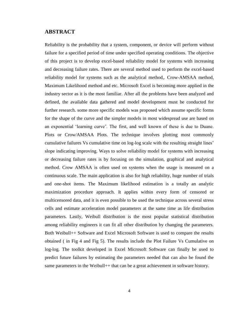
ABSTRACT
Reliability is the probability that a system, component, or device will perform without
failure for a specified period of time under specified operating conditions. The objective
of this project is to develop excel-based reliability model for systems with increasing
and decreasing failure rates. There are several method used to perform the excel-based
reliability model for systems such as the analytical method,. Crow-AMSAA method,
Maximum Likelihood method and etc. Microsoft Excel is becoming more applied in the
industry sector as it is the most familiar. After all the problems have been analyzed and
defined, the available data gathered and model development must be conducted for
further research. some more specific models was proposed which assume specific forms
for the shape of the curve and the simpler models in most widespread use are based on
an exponential „learning curve‟. The first, and well known of these is due to Duane.
Plots or Crow/AMSAA Plots. The technique involves plotting most commonly
cumulative failures Vs cumulative time on log-log scale with the resulting straight lines‟
slope indicating improving. Ways to solve reliability model for systems with increasing
or decreasing failure rates is by focusing on the simulation, graphical and analytical
method. Crow AMSAA is often used on systems when the usage is measured on a
continuous scale. The main application is also for high reliability, huge number of trials
and one-shot items. The Maximum likelihood estimation is a totally an analytic
maximization procedure approach. It applies within every form of censored or
multicensored data, and it is even possible to be used the technique across several stress
cells and estimate acceleration model parameters at the same time as life distribution
parameters. Lastly, Weibull distribution is the most popular statistical distribution
among reliability engineers it can fit all other distribution by changing the parameters.
Both Weibull++ Software and Excel Microsoft Software is used to compare the results
obtained ( in Fig 4 and Fig 5). The results include the Plot Failure Vs Cumulative on
log-log. The toolkit developed in Excel Microsoft Software can finally be used to
predict future failures by estimating the parameters needed that can also be found the
same parameters in the Weibull++ that can be a great achievement in software history.

5
ACKNOWLEDGEMENT
All the success and praises to Allah who has given the author all the strength and
motivation needed to complete this brilliant project within the limited period of time.
Special thanks also awarded by the author to his forever beloved Supervisor Dr. Masdi
Bin Muhammad who had been the man behind all the spectacular success and endlessly
gave him more than enough support that he could never repay needed in designing this
project.
A happy and big thanks also to the graduate assistant and also to his colleagues in
Universiti Teknologi PETRONAS (UTP) that gave him a lot of support and endless
ideas which basically contributed to the development of the project.
Finally, special thanks and biggest gratitude to the authors parents and also Universiti
Teknologi PETRONAS (UTP) whom always will be loved and engraved deeply in the
heart of the author.
6
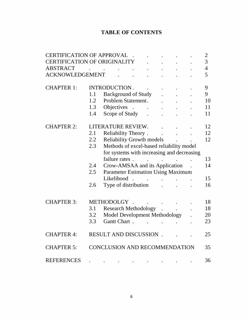
TABLE OF CONTENTS
CERTIFICATION OF APPROVAL . . . . . 2
CERTIFICATION OF ORIGINALITY . . . . 3
ABSTRACT . . . . . . . . 4
ACKNOWLEDGEMENT . . . . . . 5
CHAPTER 1: INTRODUCTION . . . . . 9
1.1 Background of Study . . . 9
1.2 Problem Statement . . . . 10
1.3 Objectives . . . . . 11
1.4 Scope of Study . . . . 11
CHAPTER 2: LITERATURE REVIEW. . . . 12
2.1 Reliability Theory . . . . 12
2.2 Reliability Growth models . . 12
2.3 Methods of excel-based reliability model
for systems with increasing and decreasing
failure rates . . . . . 13
2.4 Crow-AMSAA and its Application . 14
2.5 Parameter Estimation Using Maximum
Likelihood . . . . . 15
2.6 Type of distribution . . . 16
CHAPTER 3: METHODOLGY . . . . . 18
3.1 Research Methodology . . . 18
3.2 Model Development Methodology . 20
3.3 Gantt Chart . . . . . 23
CHAPTER 4: RESULT AND DISCUSSION . . . 25
CHAPTER 5: CONCLUSION AND RECOMMENDATION 35
REFERENCES . . . . . . . . 36
7
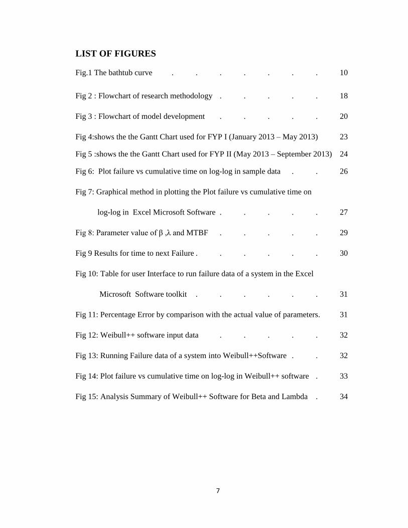
LIST OF FIGURES
Fig.1 The bathtub curve . . . . . . . 10
Fig 2 : Flowchart of research methodology . . . . . 18
Fig 3 : Flowchart of model development . . . . . 20
Fig 4:shows the the Gantt Chart used for FYP I (January 2013 – May 2013) 23
Fig 5 :shows the the Gantt Chart used for FYP II (May 2013 – September 2013) 24
Fig 6: Plot failure vs cumulative time on log-log in sample data . . 26
Fig 7: Graphical method in plotting the Plot failure vs cumulative time on
log-log in Excel Microsoft Software . . . . . 27
Fig 8: Parameter value of β ,λ and MTBF . . . . . 29
Fig 9 Results for time to next Failure . . . . . . 30
Fig 10: Table for user Interface to run failure data of a system in the Excel
Microsoft Software toolkit . . . . . . 31
Fig 11: Percentage Error by comparison with the actual value of parameters. 31
Fig 12: Weibull++ software input data . . . . . 32
Fig 13: Running Failure data of a system into Weibull++Software . . 32
Fig 14: Plot failure vs cumulative time on log-log in Weibull++ software . 33
Fig 15: Analysis Summary of Weibull++ Software for Beta and Lambda . 34
8
LIST OF TABLE
Table 1: Excel expressions for time to failure for various distributions of
interest in reliability . . . . . . . 17
Table 2: observed times between failures of a system . . . 25
Table 3: Table of Failure data input of system in Excel Microsoft Software 28
Table 4 : Table of results for parameters β and λ . . . . 29
Table 5: Results for time to next failure . . . . . 30
9
CHAPTER 1
INTRODUCTION
1.1 Background of Study
Reliability is the probability that a system, component, or device will perform without
failure for a specified period of time under specified operating conditions. George
E.Dieter, Linda C. Schmidt (2013).The importance of reduction of the likelihood or
frequency of failures must be focused by identify and make better improvements on the
root cause of failure and to find alternatives to handle failure that will occur and finally
to make data analysis on the reliability data. If an effective reliability system could be
reached then reduction of the overall cost can be made efficiently.
There are some methods used to perform the development of excel-based
reliability model for systems with increasing/decreasing failure rates using analytical
methods such as Crow-AMSAA method and Maximum likelihood method. The
Maximum likelihood estimation is a totally an analytic maximization procedure
approach. It applies within every form of censored or multicensored data, and it is even
possible to be used the technique across several stress cells and estimate acceleration
model parameters at the same time as life distribution parameters. Moreover, MLE's and
Likelihood Functions generally have very desirable large sample properties such that
they becomes unbiased minimum variance estimators as the sample size increases, have
approximate normal distributions and approximate sample variances that can be
calculated and used to generate confidence bounds. Likelihood functions can be used to
test hypotheses about models and parameters which will be useful in making system
modelling.
Crow-AMSAA method is often used on systems when the usage is measured on
a continuous scale. The main application is also for high reliability, huge number of
trials and one-shot items. The test programs are normally made on a phase by phase
basis. The fundamental understanding is that the Crow-AMSAA model is intended for
tracking the reliability within a test phase and not across test phases.
10
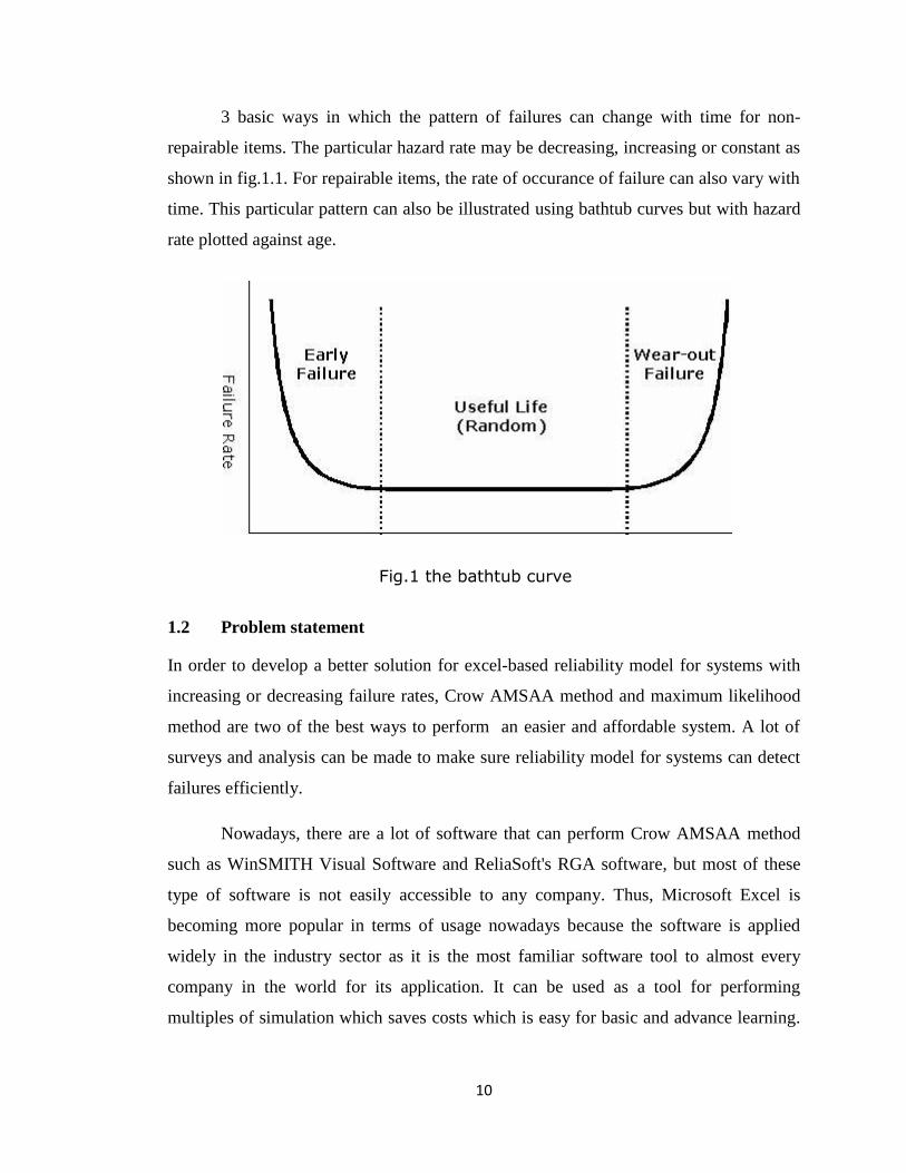
3 basic ways in which the pattern of failures can change with time for non-
repairable items. The particular hazard rate may be decreasing, increasing or constant as
shown in fig.1.1. For repairable items, the rate of occurance of failure can also vary with
time. This particular pattern can also be illustrated using bathtub curves but with hazard
rate plotted against age.
Fig.1 the bathtub curve
1.2 Problem statement
In order to develop a better solution for excel-based reliability model for systems with
increasing or decreasing failure rates, Crow AMSAA method and maximum likelihood
method are two of the best ways to perform an easier and affordable system. A lot of
surveys and analysis can be made to make sure reliability model for systems can detect
failures efficiently.
Nowadays, there are a lot of software that can perform Crow AMSAA method
such as WinSMITH Visual Software and ReliaSoft's RGA software, but most of these
type of software is not easily accessible to any company. Thus, Microsoft Excel is
becoming more popular in terms of usage nowadays because the software is applied
widely in the industry sector as it is the most familiar software tool to almost every
company in the world for its application. It can be used as a tool for performing
multiples of simulation which saves costs which is easy for basic and advance learning.
11
Big part of the society expects better planning to achieve success and rejects abnormal
$Risks in using unfamiliar software.
1.3 Objective
The objective of this project is to develop excel-based reliability model for systems with
increasing and decreasing failure rates based on Crow-AMSAA method.
1.4 Scope of Study
The scope of study relates to the development of excel-based reliability model for
systems with increasing and decreasing failure rates which uses the Reliability theory
by CROW AMSAA method. This research project will find the increasing and
decreasing failure rates in the bathtub curves that identifies whether there is an
improvement or degradation by calculating the time interval for next failure of the
reliability model system. For this project, Microsoft Excel is used for data storage and
computer simulation.
12
CHAPTER 2
LITERATURE REVIEW
2.1 Reliability theory
George E.Dieter, Linda C. Schmidt (2013) stated that “Reliability is the probability that
a system, component, or device will perform without failure for a specified period of
time under specified operating conditions”. The discipline of reliability engineering
generally is a study of the causes, distribution and prediction of failure . If R(t) is the
reliability with respect to time t, then F(t) is the unreliability(probability of failure) in the
same time t. Since failure and nonfailure are mutually exclusive events,
R(t) + F(t) =1 (14.13)
The reliability theory statement is also agreed by Patrick (2012) “Reliability is
the probability of an item will perform a required function without failure under stated
conditions for a stated period of time” which shows that it is vital to prevent or to reduce
the likelihood or frequency of failures, to identify and improve the cause of failure that
usually occur, to find ways to handling with failure that will be occur and lastly to
analyzing reliability data. If found the reliability of the system is very efficient then the
overall cost will also be reduced. [13]
2.2 Reliability Growth models
John Davidson,(1994) said that some more specific models was proposed which assume
specific forms for the shape of the curve and the simpler models in most widespread use
are based on an exponential „learning curve‟. The first, and well known of these is due
to Duane. It was derived empirically from observation of the reliability improvements
patterns of a number of electronic and mechanical systems.[16] This is basically for the
development of AMSAA model which can be differently express the basic logic model
as Duane and other more advanced models.
13
The AMSAA model assumes that the failure are the results of a NHPP which
shows that the number of failures in specified time intervals have a Poisson distribution
but Failure Rate is not constant. The object of all these models os to quantify the rate of
reduction of Failure Rate, and to predict the further development effort needed to meet
specific targets.[16]
John Davidson,(1994) works was also agreed by Nigel Comerford(2005)
technical papers which states that the Reliability Growth Plots have a variety of names,
such as Duane Plots, Crow Plots or Crow/AMSAA Plots. The technique involves
plotting most commonly cumulative failures Vs cumulative time on log-log scale with
the resulting straight lines‟ slope indicating improving , deteriorating or constant
reliability.[17] It is important to search for beta values with the basic conditions to show
the trend of failure rate in graphical methods. This method which handles mixed failure
modes can forecast future failures.
2.3 Methods of Excel-based reliability model for systems with increasing and
decreasing failure rates.
Ways to solve reliability model for systems with increasing or decreasing failure rates is
by focusing on the simulation, graphical and analytical method. The analytical approach
which applies such mathematical models for formal modelling of systems had been used
which enable analysis for future patterns of behaviours of the system. Nowadays,
computer simulation had played the most important role of making simulation model
because of the low cost ,accuracy and the validity of the simulation model. This make it
easier for industry to do their projects that saves time, energy, costs and prevents higher
risks without confronting expensive and dangerous experiments that needs lots of
materials.
Crow AMSAA method will be the best to be used for making simulation on discrete
system. The Crow-AMSAA model is designed for tracking the reliability within a test
phase and not across test phases.

14
2.4 Crow-AMSAA and its application
Crow AMSAA is often used on systems when the usage is measured on a continuous
scale. The main application is also for high reliability, huge number of trials and one-
shot items. The test programs are normally made on a phase by phase basis. The
fundamental understanding is that the Crow-AMSAA model is intended for tracking the
reliability within a test phase and not across test phases. [1]Crow AMSAA method
applies the working principles of finding the time between failure data (TBF) by
creating the β slope which is in the log summation of failure vs log summation of time
graph. Slope β is estimated by using maximum likelihood method. This is vital to detect
for increasing or decreasing failure rates for reliability model for systems which will be
calculated for predictions of every time interval for the next failure. Crow-AMSAA
model is an empirical relationship which will further into equivalent to a non-
homogeneous Poisson process (N.H.P.P.) model which will also involve a Weibull
intensity function. Furthermore, the focus on the test phases which is within a reliability
program can become equal or unequal length. Thus the Crow-AMSAA model is
focusing on the calculations of the reliability growth which is within a specific phase.
In "Reliability Analysis for Complex, Repairable Systems" (1974), Dr. Larry H.
Crow noted that the Duane model could be stochastically represented as a Weibull
process, allowing for statistical procedures to be used in the application of this model in
reliability growth. This statistical extension became what is known as the Crow-
AMSAA (NHPP) model. This method was first developed at the U.S. Army Materiel
Systems Analysis Activity (AMSAA). It is frequently used on systems when usage is
measured on a continuous scale. It can also be applied for the analysis of one shot items
when there is high reliability and large number of trials.
Test programs are generally conducted on a phase by phase basis. The Crow-
AMSAA model is designed for tracking the reliability within a test phase and not across
test phases. A development testing program may consist of several separate test phases.
If corrective actions are introduced during a particular test phase then this type of testing
and the associated data are appropriate for analysis by the Crow-AMSAA model. The
15
model analyzes the reliability growth progress within each test phase and can aid in
determining the following:
Reliability of the configuration currently on test
Reliability of the configuration on test at the end of the test phase
Expected reliability if the test time for the phase is extended
Growth rate
Confidence intervals
Applicable goodness-of-fit tests
2.5 Parameter Estimation Using Maximum Likelihood
Another method that will be used besides Crow AMSAA is the Maximum likelihood
method. The method starts by making estimation using mathematical expression of the
Likelihood Function of a sample data. likelihood set of data is the probability of
obtaining that particular set of data, which is given its chosen probability distributed
model.
The Maximum likelihood estimation is a totally an analytic maximization
procedure approach. It applies within every form of censored or multicensored data, and
it is even possible to be used the technique across several stress cells and estimate
acceleration model parameters at the same time as life distribution parameters.
Moreover, MLE's and Likelihood Functions generally have very desirable large sample
properties such that they becomes unbiased minimum variance estimators as the sample
size increases, have approximate normal distributions and approximate sample
variances that can be calculated and used to generate confidence bounds. Likelihood
functions can be used to test hypotheses about models and parameters
The method of maximum likelihood provides a basis for many of the techniques and
methods discussed in this course. The reasons are:
16
The method has a good intuitive foundation. The underlying concept is that the
best estimate of a parameter is that giving the highest probability that the
observed set of measurements will be obtained.
The least-squares method and various approaches to combining errors or
calculating weighted averages, etc., can be derived or justified in terms of the
maximum likelihood approach.
The method is of sufficient generality that most problems are amenable to a
straightforward application of this method, even in cases where other techniques
become difficult. Inelegant but conceptually simple approaches often provide
useful results where there is no easy alternative. [3]
2.6 Type of distribution
Crow-AMSAA method which uses incredible mathematical modelling and statistical
capabilities in the Excel Microsoft Software, the data will be entered into each and every
cell in the Excel based on the failure time distribution either it is lognormal, normal,
weibull distribution or exponential.
The type of distribution that is used and familiar nowadays are the Normal or
Gaussian distribution, which it is symmetric and the pattern occurs in many natural
phenomena for example temperature, rain quantity and so much more, it define the mean
o expected value and a standard variation to express the variation about the mean. While
lognormal distribution is based on normal distribution although it is not symmetric, but
it has range of shapes and it does not have normal distribution‟s disadvantage of
extending below zero.
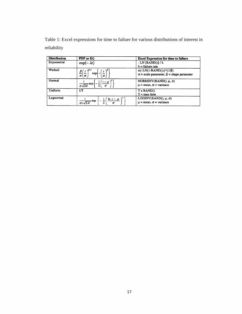
About the uniform distribution, all the values of chance of occurring and it
simply defines the minimum and maximum. For exponential distribution, it show that
the hazard rate constant. Lastly, Weibull distribution is the most popular statistical
distribution among reliability engineers it can fit all other distribution by changing the
parameters. [13]
17
Table 1: Excel expressions for time to failure for various distributions of interest in
reliability
18
CHAPTER 3
Methodology
3.1 Research Methodology
No
Yes
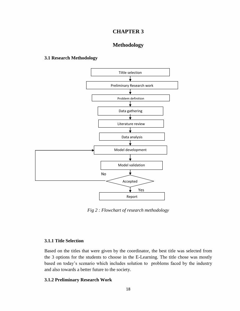
Fig 2 : Flowchart of research methodology
3.1.1 Title Selection
Based on the titles that were given by the coordinator, the best title was selected from
the 3 options for the students to choose in the E-Learning. The title chose was mostly
based on today‟s scenario which includes solution to problems faced by the industry
and also towards a better future to the society.
3.1.2 Preliminary Research Work
Model validation
Preliminary Research work
Tiltle selection
Problem definition
Literature review
Data gathering
Data analysis
Model development
Report
Accepted
< < <
19
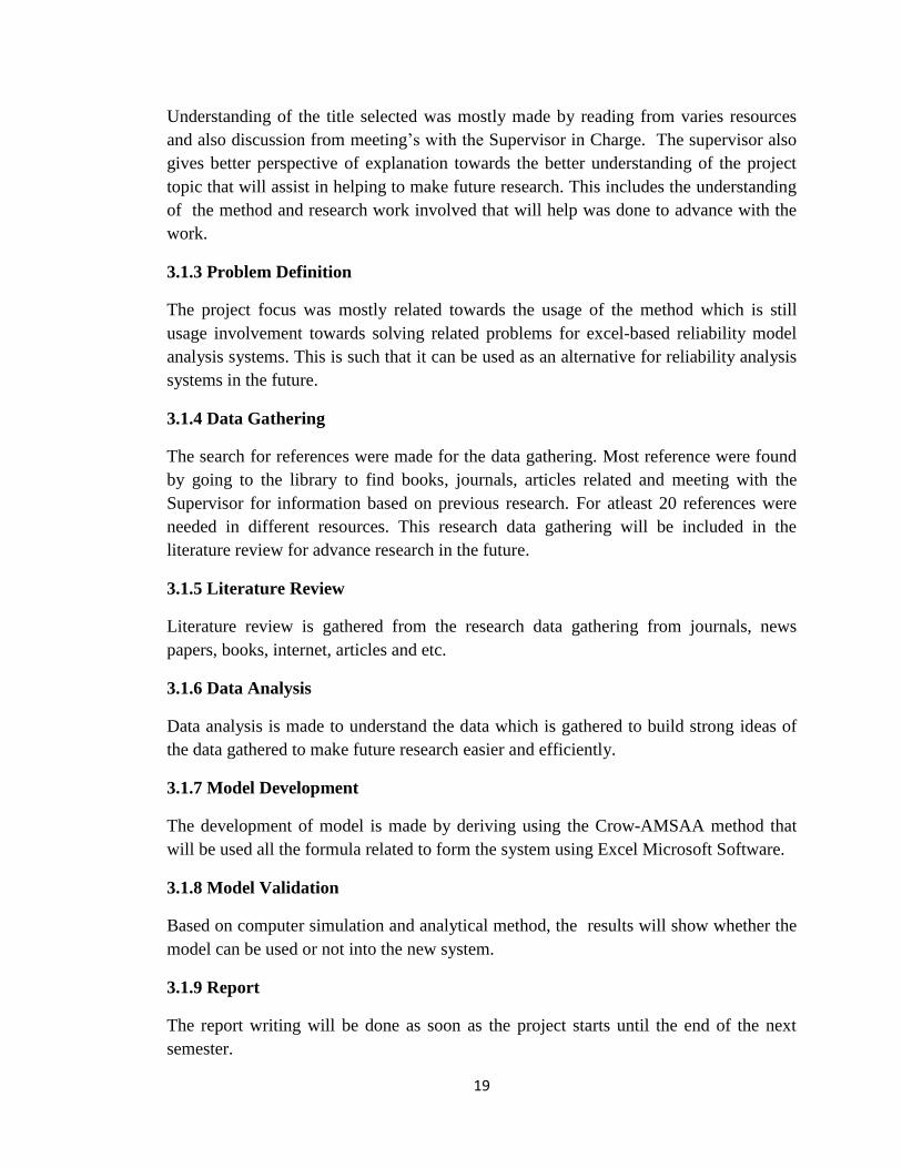
Understanding of the title selected was mostly made by reading from varies resources
and also discussion from meeting‟s with the Supervisor in Charge. The supervisor also
gives better perspective of explanation towards the better understanding of the project
topic that will assist in helping to make future research. This includes the understanding
of the method and research work involved that will help was done to advance with the
work.
3.1.3 Problem Definition
The project focus was mostly related towards the usage of the method which is still
usage involvement towards solving related problems for excel-based reliability model
analysis systems. This is such that it can be used as an alternative for reliability analysis
systems in the future.
3.1.4 Data Gathering
The search for references were made for the data gathering. Most reference were found
by going to the library to find books, journals, articles related and meeting with the
Supervisor for information based on previous research. For atleast 20 references were
needed in different resources. This research data gathering will be included in the
literature review for advance research in the future.
3.1.5 Literature Review
Literature review is gathered from the research data gathering from journals, news
papers, books, internet, articles and etc.
3.1.6 Data Analysis
Data analysis is made to understand the data which is gathered to build strong ideas of
the data gathered to make future research easier and efficiently.
3.1.7 Model Development
The development of model is made by deriving using the Crow-AMSAA method that
will be used all the formula related to form the system using Excel Microsoft Software.
3.1.8 Model Validation
Based on computer simulation and analytical method, the results will show whether the
model can be used or not into the new system.
3.1.9 Report
The report writing will be done as soon as the project starts until the end of the next
semester.
20
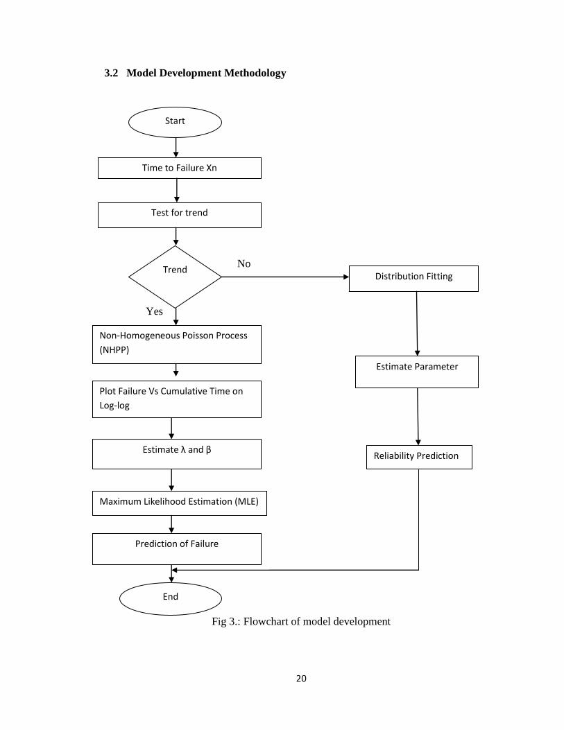
3.2 Model Development Methodology
No
Yes
Fig 3.: Flowchart of model development
Time to Failure Xn
Test for trend
Trend
Non-Homogeneous Poisson Process
(NHPP)
Plot Failure Vs Cumulative Time on
Log-log
Estimate λ and β
Distribution Fitting
Estimate Parameter
Reliability Prediction
Maximum Likelihood Estimation (MLE)
Prediction of Failure
End
Start

21
3.2.1. Time to failure Xn;
In this first part in the methodology, the cumulative time parameters for the time to
failure is determined from the data set for the Crow/AMSAA Reliability Growth Plots.
It is important to determine and receive the cumulative time to failure data so that it can
be used for the test for trend.
3.2.2. Test for Trend
Test for trend is determined in this methodology by using 2 major methods which can
determine whether the set of data is decreasing, increasing or even no trend in failure by
making the Plot Failure vs Cumulative Time on log-log by using either the distributing
fitting or Non-Homogeneous Poisson Process.
3.2.3.1 If Trend
3.2.3.1.1 NHPP
If there is a trend, the Prediction of Failure can be made through the Non-Homogeneous
Poisson Process which mathematical models were involved. Such mathematical model
used are the intensity function ρ(t), the log of the cumulative failure events n(t), natural
logarithms Lnn(t), the cumulative failure rate C(t), The λ and β values is gained from the
Plot Failure Vs Cumulative Time on log-log.
3.2.3.1.2. Plot Failure Vs Cumulative Time on log-log.
This Plot Failure Vs Cumulative Time on log-log is accomplished by using Excel
Microsoft Software. This step is made in the methodology so that it can be compared the
results gained with the Weibull++ Software.
3.2.3.1.3. Estimate λ and β.
The values for λ and β can be determined from the Failure vs Cumulative Time on log-
log plot. These values then can be included in the mathematical models to be used in the
Crow-AMSAA method.
3.2.3.1.4. Maximum Likelihood Method
For futher developments, Maximum Likelihood Estimates is useful in determining
lambda and beta from which p(t) and C(t) can be derived. This method is used with time
and failure terminated data or interval and group data. It describes an unbiased method
for determining the parameters suitable for use when the individual failure times are
known. Paul Barringer investigated the accuracy of all three methods, Rank Regression,

22
MLE, and IEC, with IEC being the best bearing in mind it requires the failure times to
be known. However it should be noted that at least 20 data points are required for any
method to work.
\
3.2.3.1.5. Prediction of Failure
Prediction of failure can be finally made as the last remaining step for the Crow-
AMSAA method. From the calculations made in the NHPP, parameters and trend tests
received from the Plot Failure Vs Cummulative Time on Log-log and MLE, the
predictions of failure in the future is easier to analyze.
3.2.3.2. If no Trend.
3.2.3.2.1. Distribution Fitting
The distribution fitting involves the usage of Weibull++ software and exponential
lognormal, where the plot Failure Vs cumulative time on log-log where the shape of the
graph can be determined whether the data has a decreasing failure rate trend or
increasing failure rate trend or even no trend.
3.2.3.2.2. Estimate parameter
From the plot of failure vs cumulative time on log-log, the parameters can be estimated
from the Weibull++ software for the λ and β values which is easy to analyze and
important for the reliability prediction process.
3.2.3.2.3. Reliability Prediction
From the values of the λ and β that had been estimated, the reliability prediction can be
made from the trend test of the Plot Failure vs Cummulative time from the Weibull++
Software which shows all the needed parameters including λ and β values.
23
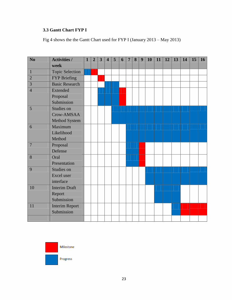
3.3 Gantt Chart FYP I
Fig 4 shows the the Gantt Chart used for FYP I (January 2013 – May 2013)
No Activities /
week
1 2 3 4 5 6 7 8 9 10 11 12 13 14 15 16
1 Topic Selection
2 FYP Briefing
3 Basic Research
4 Extended
Proposal
Submission
5 Studies on
Crow-AMSAA
Method System
6 Maximum
Likelihood
Method
7 Proposal
Defense
8 Oral
Presentation
9 Studies on
Excel user
interface
10 Interim Draft
Report
Submission
11 Interim Report
Submission
24
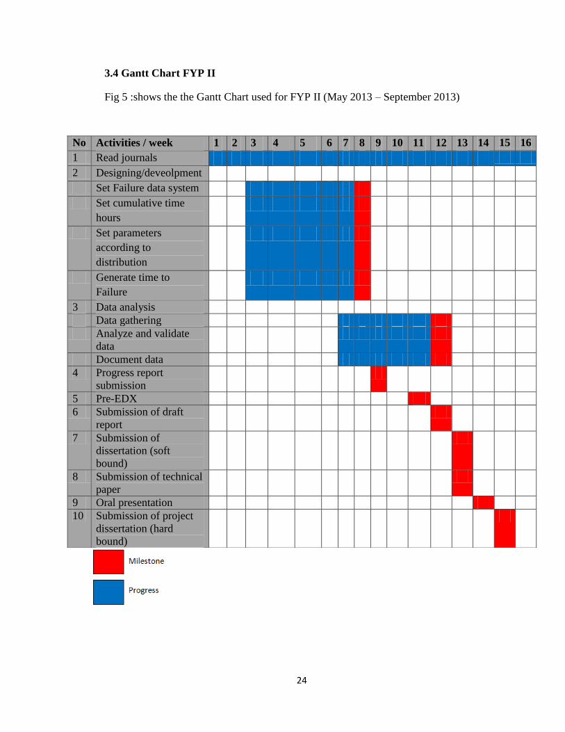
3.4 Gantt Chart FYP II
Fig 5 :shows the the Gantt Chart used for FYP II (May 2013 – September 2013)
No Activities / week 1 2 3 4 5 6 7 8 9 10 11 12 13 14 15 16
1 Read journals
2 Designing/deveolpment
Set Failure data system
Set cumulative time
hours
Set parameters
according to
distribution
Generate time to
Failure
3 Data analysis
Data gathering
Analyze and validate
data
Document data
4 Progress report
submission
5 Pre-EDX
6 Submission of draft
report
7 Submission of
dissertation (soft
bound)
8 Submission of technical
paper
9 Oral presentation
10 Submission of project
dissertation (hard
bound)
25
CHAPTER 4
Result and Discussion
In this particular project, the results gained is by making a simulation using both Excel
Microsoft software to be compared with the Weibull ++ software. The finding was
absolutely magnificent as months of research and development the results had finally
been awarded to this project. The simulation results were guided and gained by using
sample sets of data used as follows[18] :
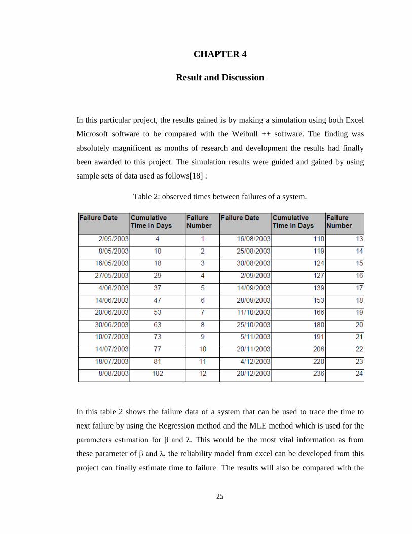
Table 2: observed times between failures of a system.
In this table 2 shows the failure data of a system that can be used to trace the time to
next failure by using the Regression method and the MLE method which is used for the
parameters estimation for β and λ. This would be the most vital information as from
these parameter of β and λ, the reliability model from excel can be developed from this
project can finally estimate time to failure The results will also be compared with the
26
Weibull++ Software as the results obtained starts from Fig 5. The results include the
Plot Failure Vs Cumulative on log-log.
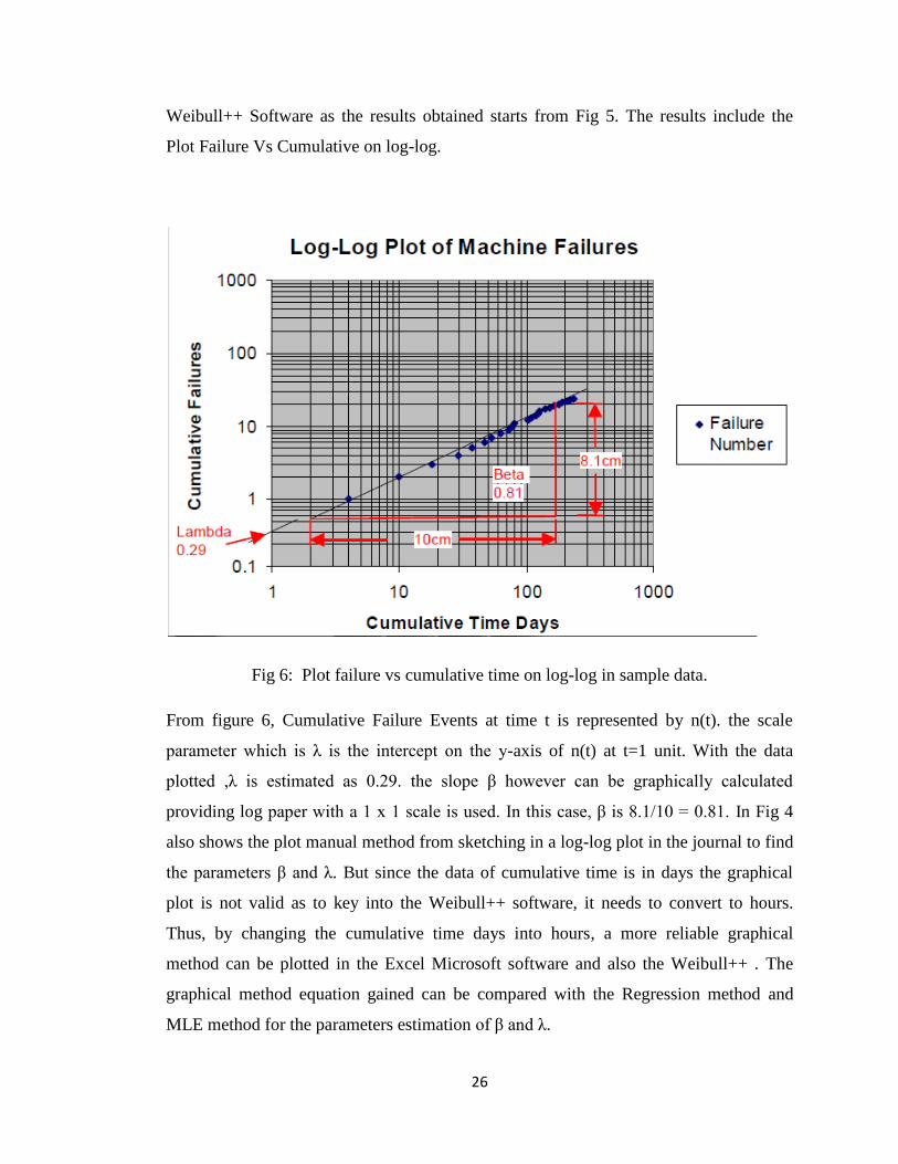
Fig 6: Plot failure vs cumulative time on log-log in sample data.
From figure 6, Cumulative Failure Events at time t is represented by n(t). the scale
parameter which is λ is the intercept on the y-axis of n(t) at t=1 unit. With the data
plotted ,λ is estimated as 0.29. the slope β however can be graphically calculated
providing log paper with a 1 x 1 scale is used. In this case, β is 8.1/10 = 0.81. In Fig 4
also shows the plot manual method from sketching in a log-log plot in the journal to find
the parameters β and λ. But since the data of cumulative time is in days the graphical
plot is not valid as to key into the Weibull++ software, it needs to convert to hours.
Thus, by changing the cumulative time days into hours, a more reliable graphical
method can be plotted in the Excel Microsoft software and also the Weibull++ . The
graphical method equation gained can be compared with the Regression method and
MLE method for the parameters estimation of β and λ.
27
Excel Microsoft Sofware
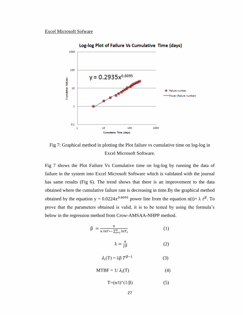
Fig 7: Graphical method in plotting the Plot failure vs cumulative time on log-log in
Excel Microsoft Software.
Fig 7 shows the Plot Failure Vs Cumulative time on log-log by running the data of
failure in the system into Excel Microsoft Software which is validated with the journal
has same results (Fig 6). The trend shows that there is an improvement to the data
obtained where the cumulative failure rate is decreasing in time.By the graphical method
obtained by the equation y = 0.0224 power line from the equation n(t)= λ . To
prove that the parameters obtained is valid, it is to be tested by using the formula‟s
below in the regression method from Crow-AMSAA-NHPP method.
(1)
(2)
(T) = λβ (3)
MTBF = 1/ (T) (4)
T=(n/t)^(1/β) (5)
28
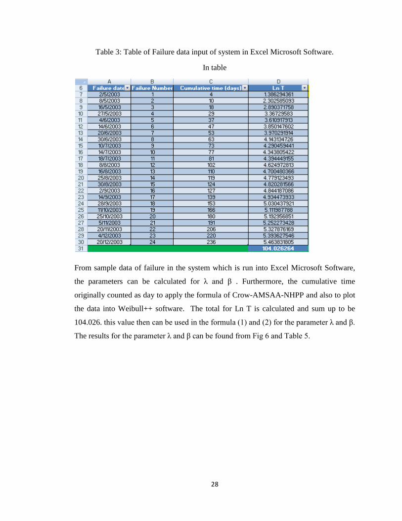
Table 3: Table of Failure data input of system in Excel Microsoft Software.
In table
From sample data of failure in the system which is run into Excel Microsoft Software,
the parameters can be calculated for λ and β . Furthermore, the cumulative time
originally counted as day to apply the formula of Crow-AMSAA-NHPP and also to plot
the data into Weibull++ software. The total for Ln T is calculated and sum up to be
104.026. this value then can be used in the formula (1) and (2) for the parameter λ and β.
The results for the parameter λ and β can be found from Fig 6 and Table 5.
29
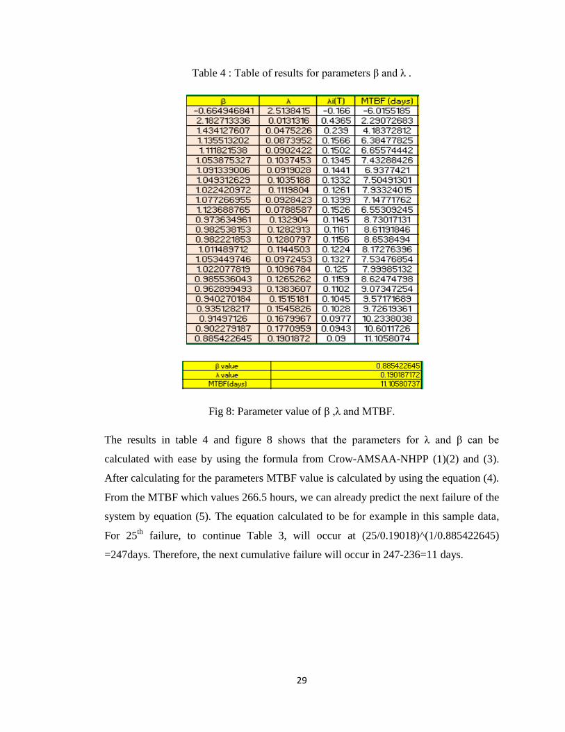
Table 4 : Table of results for parameters β and λ .
Fig 8: Parameter value of β ,λ and MTBF.
The results in table 4 and figure 8 shows that the parameters for λ and β can be
calculated with ease by using the formula from Crow-AMSAA-NHPP (1)(2) and (3).
After calculating for the parameters MTBF value is calculated by using the equation (4).
From the MTBF which values 266.5 hours, we can already predict the next failure of the
system by equation (5). The equation calculated to be for example in this sample data,
For 25th
failure, to continue Table 3, will occur at (25/0.19018)^(1/0.885422645)
=247days. Therefore, the next cumulative failure will occur in 247-236=11 days.
30
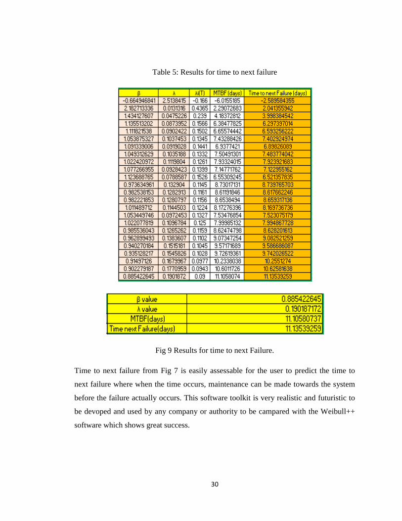
Table 5: Results for time to next failure
Fig 9 Results for time to next Failure.
Time to next failure from Fig 7 is easily assessable for the user to predict the time to
next failure where when the time occurs, maintenance can be made towards the system
before the failure actually occurs. This software toolkit is very realistic and futuristic to
be devoped and used by any company or authority to be campared with the Weibull++
software which shows great success.
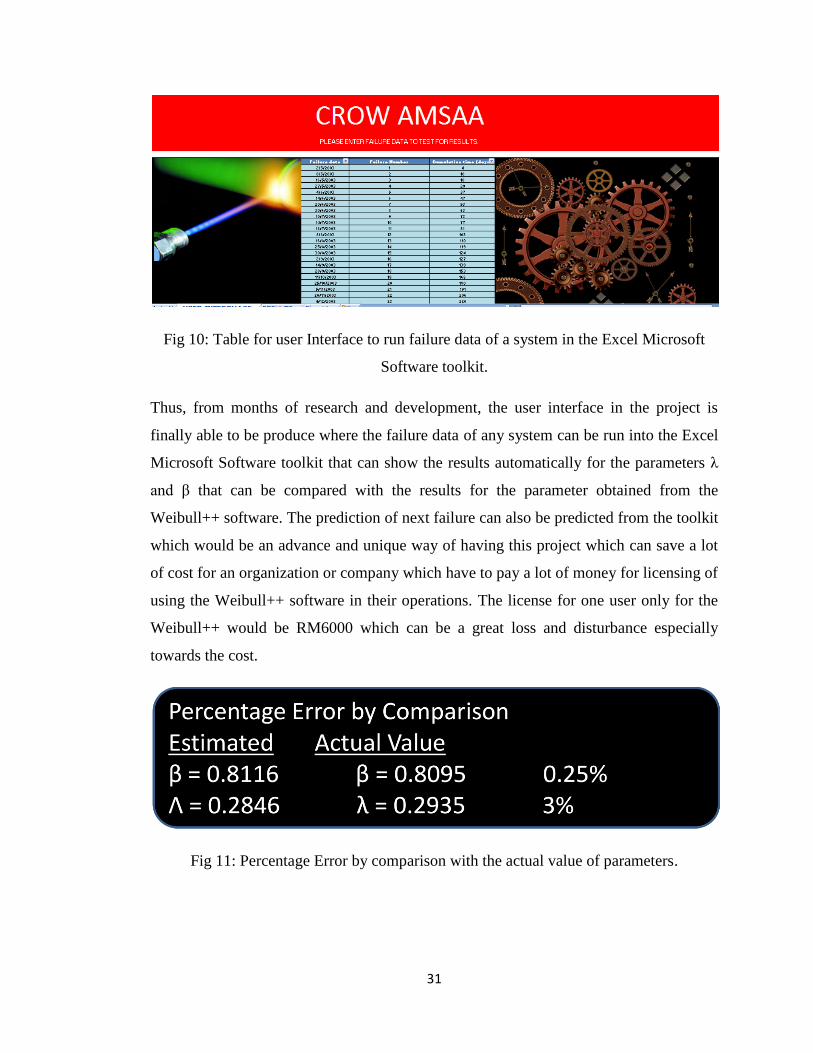
31
Fig 10: Table for user Interface to run failure data of a system in the Excel Microsoft
Software toolkit.
Thus, from months of research and development, the user interface in the project is
finally able to be produce where the failure data of any system can be run into the Excel
Microsoft Software toolkit that can show the results automatically for the parameters λ
and β that can be compared with the results for the parameter obtained from the
Weibull++ software. The prediction of next failure can also be predicted from the toolkit
which would be an advance and unique way of having this project which can save a lot
of cost for an organization or company which have to pay a lot of money for licensing of
using the Weibull++ software in their operations. The license for one user only for the
Weibull++ would be RM6000 which can be a great loss and disturbance especially
towards the cost.
Fig 11: Percentage Error by comparison with the actual value of parameters.
32
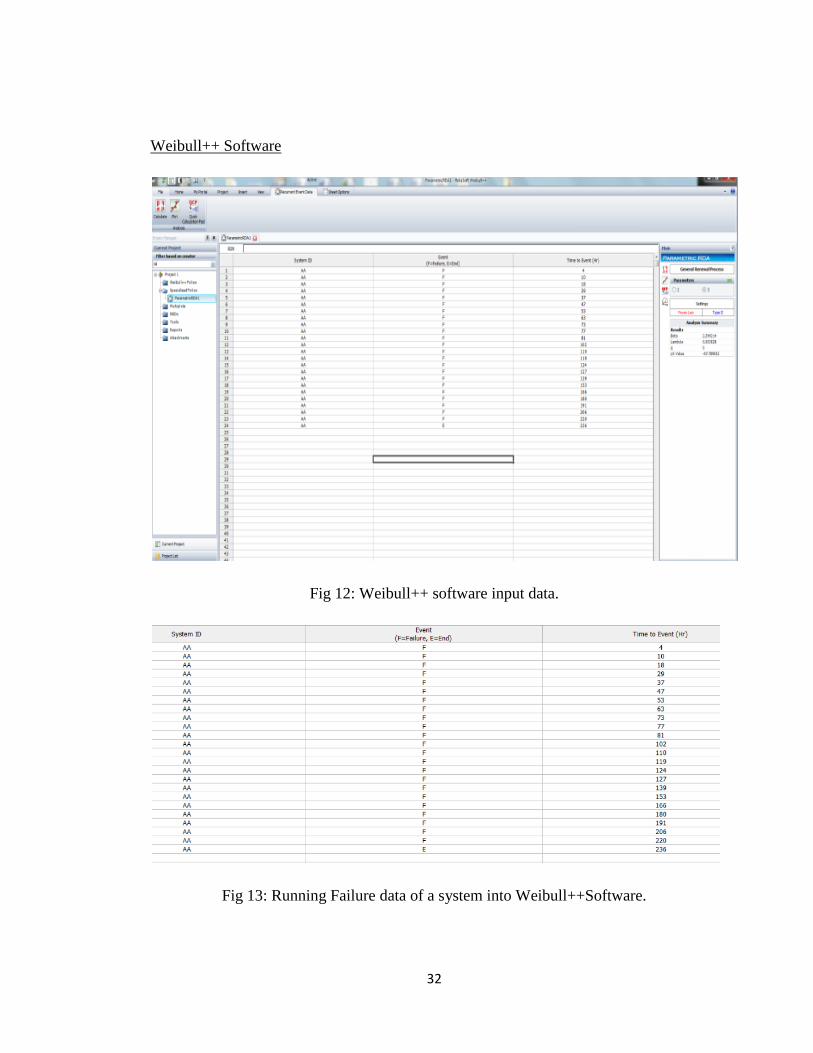
Weibull++ Software
Fig 12: Weibull++ software input data.
Fig 13: Running Failure data of a system into Weibull++Software.
33
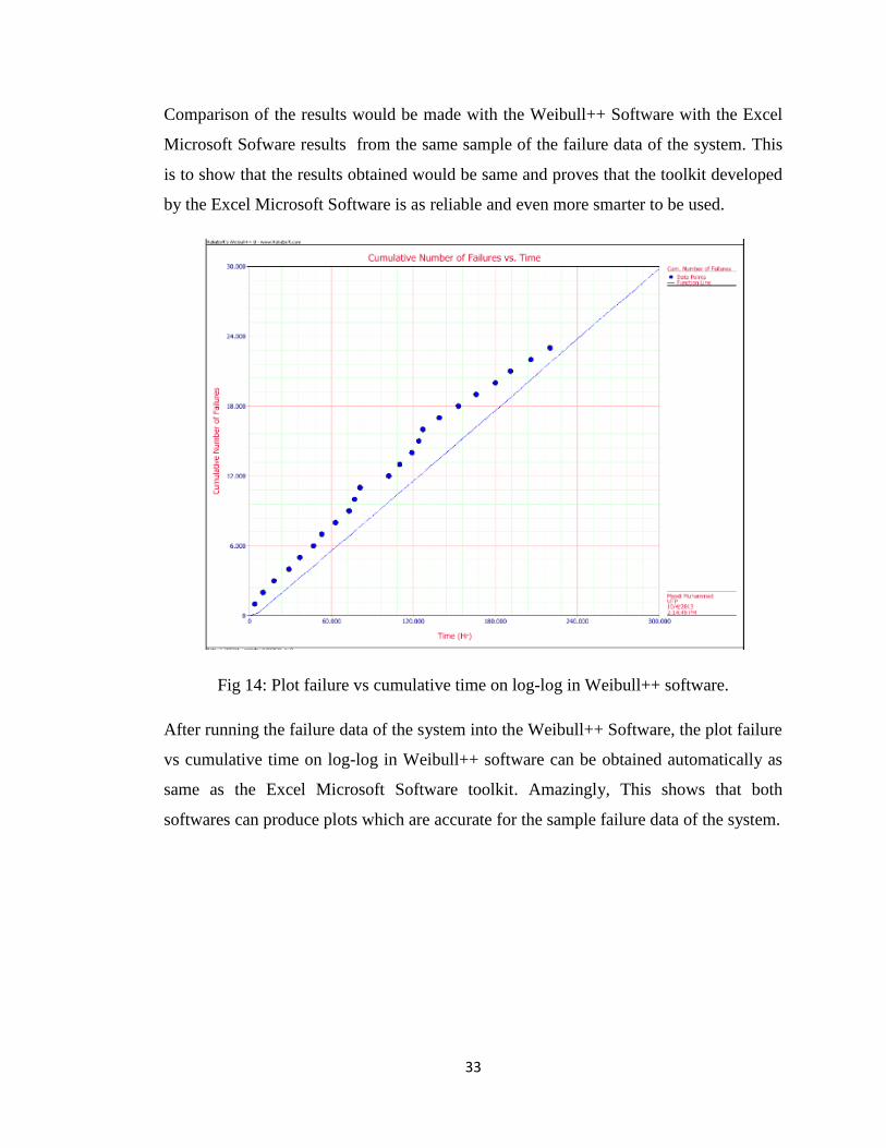
Comparison of the results would be made with the Weibull++ Software with the Excel
Microsoft Sofware results from the same sample of the failure data of the system. This
is to show that the results obtained would be same and proves that the toolkit developed
by the Excel Microsoft Software is as reliable and even more smarter to be used.
Fig 14: Plot failure vs cumulative time on log-log in Weibull++ software.
After running the failure data of the system into the Weibull++ Software, the plot failure
vs cumulative time on log-log in Weibull++ software can be obtained automatically as
same as the Excel Microsoft Software toolkit. Amazingly, This shows that both
softwares can produce plots which are accurate for the sample failure data of the system.
34
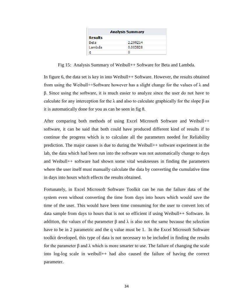
Fig 15: Analysis Summary of Weibull++ Software for Beta and Lambda.
In figure 6, the data set is key in into Weibull++ Software. However, the results obtained
from using the Weibull++Software however has a slight change for the values of λ and
β. Since using the software, it is much easier to analyze since the user do not have to
calculate for any interception for the λ and also to calculate graphically for the slope β as
it is automatically done for you as can be seen in fig 8.
After comparing both methods of using Excel Microsoft Software and Weibull++
software, it can be said that both could have produced different kind of results if to
continue the progress which is to calculate all the parameters needed for Reliability
prediction. The major causes is due to during the Weibull++ software experiment in the
lab, the data which had been run into the software was not automatically change to days
and Weibull++ software had shown some vital weaknesses in finding the parameters
where the user itself must manually calculate the data by converting the cumulative time
in days into hours which effects the results obtained.
Fortunately, in Excel Microsoft Software Toolkit can be run the failure data of the
system even without converting the time from days into hours which would save the
time of the user. This would have been time consuming for the user to convert lots of
data sample from days to hours that is not so efficient if using Weibull++ Software. In
addition, the values of the parameter β and λ is also not the same because the selection
have to be in 2 parametric and the q value must be 1. In the Excel Microsoft Software
toolkit developed, this type of data is not necessary to be included in finding the results
for the parameter β and λ which is more smarter to use. The failure of changing the scale
into log-log scale in weibull++ had also caused the failure of having the correct
parameter.
35
CHAPTER 5:
Conclusion & Recommendation
Conclusion
The simulation test was a success as the parameters for β and λ was gained from the
from the from the Excel Microsoft Software toolkit. These parameters is useful to be
used in Trend test on the failure rates whether increasing or decreasing. It is also useful
to be used in some mathematical model for reliability prediction in the future. FYP II
concentrates especially on the fantastic results obtained and literature review part where
most of the sources were gained successfully.
Recommendation
Based on the results obtained, the development of this project can be enhanced in the
coming future with greater achievements as more application can be included. The
toolkit can also be improved by having more parameters for failure numbers to be key in
into it that can calculate for even more than 10 years calculation data which can be great
to achieve in the future. Hopefully more research can be continued to be done in this
project title as more time is actually needed to gain greater yet more impressive results.
36
REFERENCE
[1] http://www.weibull.com/hotwire/issue49/relbasics49.htm retrieved on 14/2/2013
[2] http://www.barringer1.com/nov02prb.htm retrieved on 13/2/2013
[3] http://www.asp.ucar.edu/colloquium/1992/notes/part1/node20.html retrieved on
12/2/2013
[4] Paul Barringer, P.E. (2004), Predict Failures: Crow-AMSAA 101 and Weibull 101,
Proceedings of IMEC (2004), International Mechanical Engineering Conference
December 5-8, 2004, Kuwait.
[5] Larry H. Crow, Ph.D. Crow (2011), Reliability Resources: Practical Methods for
Analyzing the Reliability of Repairable Systems
[6] Huairui Guo, Ph.D., ReliaSoft Corporation , Wenbiao Zhao, Ph.D., American
Express Adamantios Mettas, ReliaSoft Corporation (2006) : Practical Methods for
Modelling Repairable w Systems with Time Trends and Repair Effects.
[7] H. Paul Barringer, P.E. (2004): Use Crow-AMSAA Reliability Growth Plots To
Forecast Future System Failures.
[8]Tadashi Dohi ,Won Young Yun (2004) ,Advanced Reliability Modelling,
Proceedings of the 2004 Asian International Workshop(AIWARM 2004) Hiroshima,
Japan 26-27 August 2004.
[9]George E.Dieter, Linda C. Schmidt ,(2013) Engineering Design ,Fifth Edition,
McGraw-Hill Companies, Inc.,1221 Avenue of the Americas, New York ,NY 10020.
[10]Arnljot Hoyland, Marvin Rausand, (1994) System Reliability Theory Models and
Statistical Methods, John Wiley & Sons, Inc., 605 Third Avenue, New York,NY 10158-
0012.
[11] JD Andrews, TR Moss (2002), Reliability and Risk Assessment Second Edition,
Professional Engineering Publishing Limited, Northgate Avenue, Bury St Edmunds,
Suffolk, IP32 6BW, UK.
[12] Mikell P. Groover (2008), Automation Production Systems , and Computer-
Integrated Manufacturing Third Edition, Pearson Education Inc. Upper Saddle River,
New Jersey 07458.

37
[13] Wallace R. Blischke, D.N. Prabhakar Murthy,(2003), Case Studies in Reliability
and Maintenance, John Wiley & Sons,Inc., Hoboken, New Jersey.
[14] R.C. Mishra, 2006, Reliability and Maintainance Engineering, (2006), New Age
International (P) Ltd., New Delhi.
[15] Patrick D.T.O‟Connor, Andre Kleyner(2012), Practical Reliability Engineering,
New York, John Wiley & Sons.
[16] John Davidson (1994),The Reliabilty of Mechanical Systems, Mechanical
Engineering Publicaation Limited, PO Box 24, Northgate Avenue, Bury St Edmunds,
Suffolk IP32 6BW.
[17] Nigel Comerford,(2005), Crow/AMSAA Reliability Growth Plots, 4.0, page 5.
[18] http://www.plant-maintenance.com/articles/Crow-AMSAA.pdf retrieved on
15/3/2013

38