2

SUPERVISOR’S DECLARATION

I hereby declare that I have checked this project and in my opinion, this project is

adequate in terms of scope and quality for the award of the degree of Bachelor of

Mechanical Engineering.

Signature

Name of Supervisor: MUHAMAD ZUHAIRI BIN SULAIMAN

Position: LECTURER

Date: 21 NOVEMBER 2009

3

STUDENT’S DECLARATION

I hereby declare that the work in this project is my own except for quotations and

summaries which have been duly acknowledged. The project has not been accepted for

any degree and is not concurently submitted for award of other degree.

Signature:

Name: PYLLISCIA SUMBOK AK ADAN

ID Number: MA06077

Date: 21 NOVEMBER 2009

4

ACKNOWLEDGEMENTS

I am grateful for finally completed this thesis and would like to take this

opportunity to express my sincere gratitude to many people that had supported and

accompanied me throughout my thesis work. This thesis had become easier to

completed as they had been together with me along my ups and down.

First, to my former supervisor En. Mohd Rosdzimin Abdul Rahman, for his

endless support, ideas, continuous motivation and invaluable guidance, in making this

research possible. He has a really thoughtful mind and his kindness for teaching and

providing me with relevance information until I fully understand my thesis was very

appreciated. I also appreciate him for believing me and achnowledging the importance

of these thesis.

My sincere gratitude also goes to my second supervisor, En. Muhamad Zuhairi

bin Sulaiman who had guide me on completing this thesis right in time. Thanks to his

effort for sharing with me the incredibly time-consuming process for creating a thesis.

Thanks again for giving me the space, time and emotional support I needed to follow

my passion and complete what must have seemed like an endless task. I also sincerely

thanks him for the time spent for reading and correcting my many mistakes.

My sincere thanks also go to all my friends for giving me extensive feedback

and invalueable suggestion for improving the first presentation and draft of this thesis. I

deeply appreciate their incrediable ability to take everything the roughest of me and

make it all work. Thanks for the way you make a significant different.

I acknowledge my sincere indebtedness and gratitude to my parents for always

being there on the phone for countless hours when I needed support and advice about

everything. Your dedication and hard support had never cease to fill my heart with

gratitude. Thanks again for being so lovely and caring.

Thank you all for your vision, caring, commitment and heartful action.

5

ABSTRACT

The aim of this thesis is to study the methods of the lattice Boltzmann equations in

order to be apply in two types of D2Q4 model in thermal fluid flow problems. LBM

has been found to be useful in application involving interfacial dynamics and complex

boundaries. These methods utilize the statistical mechanics of simple discrete models to

simulate complex physical systems. The theory of lattice Boltzmann method in nine and

four velocity model are reviewed. The isothermal and thermal equation have been

derived from the Boltzmann equation by descretiziton on both time and phase space. In

this isothermal problem, a few simple isotherml flow simulation will be done by using

the nine velocity model. The concepts of distribution function are considered beside the

theory of Boltzmann equations. Then the derivations of Navier-Stokes equation from

the Boltzmann equations are also presented. Some simulation results are performed, to

highlight the important features of the isothermal LB model. The application of lattice

Boltzmann scheme in thermal fluid problem is investigated in chapter 3. By using the

derivation of the discretised density distribution function, a 4-velocity model is applied

to develop the internal energy distribution function. This model is validated to simulate

the porous couette flow problem for thermal fluid flow problems. The performance for

both types D2Q4 microscopic model is demonstrated in the simulations of porous

thermal couette flow and natural convection flow in a square cavity. The simulation of

thermal fluids flow is applied to two different types of four-velocity model that are

Azwadi model and old model. The same simulation test is performed for both types and

the accuracy and stability analysis of both models are stated. These models are

compared and discussed to ensure its validity.

6

ABSTRAK

Tujuan utama tesis ini adalah untuk mempelajari kaedah kekisi Boltzmann yang akan

diaplikasikan pada dua jenis halaju model D2Q4 di dalam masalah terma. Kaedah kekisi

Boltzmann telah pun diketahui berguna di dalam aplikasi yang membabitkan

perhubungan di antara dinamik dan sempadan yang rumit. Algoritma ini adalah mudah

dan dapat dilaksanakan pada intisari sesuatu model dengan mengunakan beberapa ratus

garisan. Kaedah ini menggunakan mekanik statik pada modal berasingan yang mudah

hingga kepada yang kompleks. Teori kekisi Boltzmann ini akan dikaji pada halaju

model empat dan sembilan hala. Persamaan isoterma dan terma diperolehi daripada

persamaan Boltzmann dengan mendekritasikan masa dan juga ruang fasa. Kemudian

masalah isoterma akan menjadi fokus utama pada awal bab ketiga. Dalam masalah

isoterma ini, beberapa simulasi mudah akan dijalankan dengan menggunakan halaju

model sembilan. Konsep pengagihan fungsi akan di pertimbangkan disamping teori

persamaan Boltzmann. Kemudian, terbitan persamaan Navier Stokes daripada

persamaan Boltzmann akan turut diperkenalkan. Beberapa keputusan simulasi

ditunjukkan bagi membuktikan kepentingan modal isoterma kaedah kekisi Boltzmann.

Seterusnya aplikasi kekisi Boltzmann akan dikaji dalam bab ketiga. Dengan

menggunakan menterbitan fungsi pengagihan tenaga, satu model empat halaju akan

digunakan untuk menghasilkan fungsi pengagihan tenaga dalaman. Model ini sahih

untuk simulasi masalah pengaliran porous coutte dalam masalah terma. Hasil prestasi

kedua-dua model D2Q4 akan dilakukan pada simulasi pengaliran porous coutte dan

pengaliran pemanasan semulajadi pada ruang segiempat. Simulasi ini akan dijalankan

ada model lama dan juga model azwadi. Ujian simulasi yang sama akan dilakukan pada

kedua-dua model dan analisis ketepatan serta kestabilan kedua-dua model akan

dibincangkan. Model ini akan dinilai dan diuji untuk membezakan prestasi kedua-dua

model.

7

TABLE OF CONTENTS

Page

SUPERVISOR’S DECLARATION ii

STUDENT’S DECLARATION iii

ACKNOWLEDGEMENTS iv

ABSTRACT v

ABSTRAK vi

TABLE OF CONTENTS vii

LIST OF TABLES x

LIST OF FIGURES xi

LIST OF SYMBOLS xiii

LIST OF ABBREVIATIONS xv

CHAPTER 1 INTRODUCTION 1

1.1 Introduction 1

1.1.1 Navier-Stokes equations 1 1.1.2. Lattice Boltzmann Method (LBM) 2

1.2 Problem Background 3

1.2.1 Project Objective 3 1.2.2 Project Scopes 3

1.3 Thesis Outline 4

CHAPTER 2 LITERATURE REVIEW 5

2.1 Lattice Boltzmann Method 5

2.2 Collision Intergral, Ω( f ) 7

2.3 BGK (Bhatnagar, Gross and Krook) 8

2.4 Boundary Condition 8

2.4.1 Periodic boundary condition 9

2.4.2 Bounce Back Boundary condition 9

8

2.5 Discretization on Microscopic Velocity Model 10

2.5.1. Isothermal Fluid Flow 10

2.5.1.1 The Macroscopic Equation for Isothermal 11

2.5.2 Thermal Fluid Flow 11

2.5.2.1. The Macroscopic Equation for Thermal 12

2. 6 Reynold Number 12

2.7 Rayleigh Number 13

2.8 Prandtl Number 15

CHAPTER 3 METHODOLOGY 16

3.1 Flow Chart 16

3.2 Algorithm 17

3.3 Simulation Result for Isothermal Flow 18

3.3.1 Poiseulle flow 18 3.3.2 Couette flow 19 3.4 Simulation Result for Thermal Flow 20

3.4.1 Thermal Porous Couette Flow

3.5 Old Velocity Model versus Azwadi’s Velocity Model 21

3.5.1 Old Velocity Model 21 3.5.2 Azwadi’s Velocity Model 22 3.6 Summary 22

CHAPTER 4 RESULTS AND DISCUSSION 23

4.1 Natural Convection in Square Cavity 23

4.2 Grid Dependency Test 24

4.3 Nusselt Number Comparison 25

4.4 Old model result versus Azwadi’s model result 26

CHAPTER 5 CONCLUSIONS AND RECOMMENDATION 29

5.1 Conclusions 29

5.2 Recommendation 30

9

REFERENCES 31

APPENDICES 32

A 1 Gantt Chart for Final Year Project 1 32

A1 Gantt Chart for Final Year Project 2 33

B Azwadi Model Simulation 34

C Old Model Simulation

10

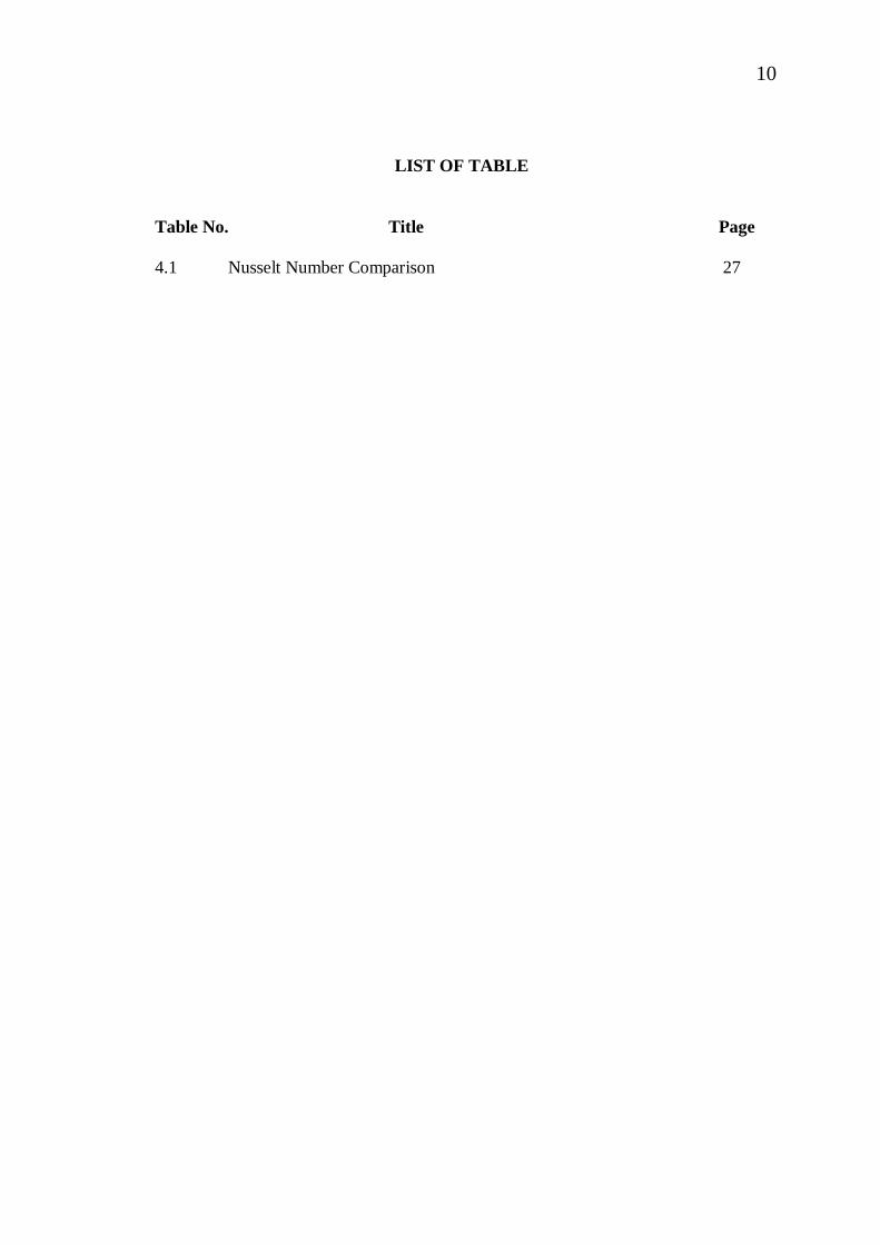
LIST OF TABLE

Table No. Title Page

4.1 Nusselt Number Comparison 27

11

LIST OF FIGURE

Figure No. Title

Page 2.1 Lattice Boltzmann Theory 6

1.2 Periodic Boundary Condition 9

2. 3 9-Discrete Velocity Model 10

2.4 4-Discrete Velocity Model 11

3.1 Flowchart for methodology 16

3.2 Original LBM Algorithm Flowchart. 17

3.3 Graph of Poiseulle Flow 18

3.4 Graph of Couette Flow 19

3.5 Temperature Profile at Pr= 0.71 and Ra= 100 20

3.6 Temperature Profile at Ra=100 and Re=10. 21

3.7 2 D Lattice structure of old velocity model 21

3.8 2 D Lattice Structure of Azwadi velocity model 22

3.9 Ghantt Chart for Final Year Project 1 23

3.10 Ghantt Chart for Final Year Project 2 24

4.1 Schematic Diagram for natural convection in a square cavity 25

4.2 Grid dependence test for Old model at Ra = 104 and Pr = 0.71 26

4.3 Grid dependence test for Azwadi model at Ra = 104 and Pr = 0.71 26

4.4 Equivalent state for Azwadi model at Ra = 103 ~ 10

5 28

4.5 Equivalent state for Old model at Ra = 103 ~ 10

5 28

4.6: Isotherms state for Azwadi's Model at Ra = 103~10

5 29

4.7 Isotherms state for Old‟s Model at Ra = 103~10

5 29

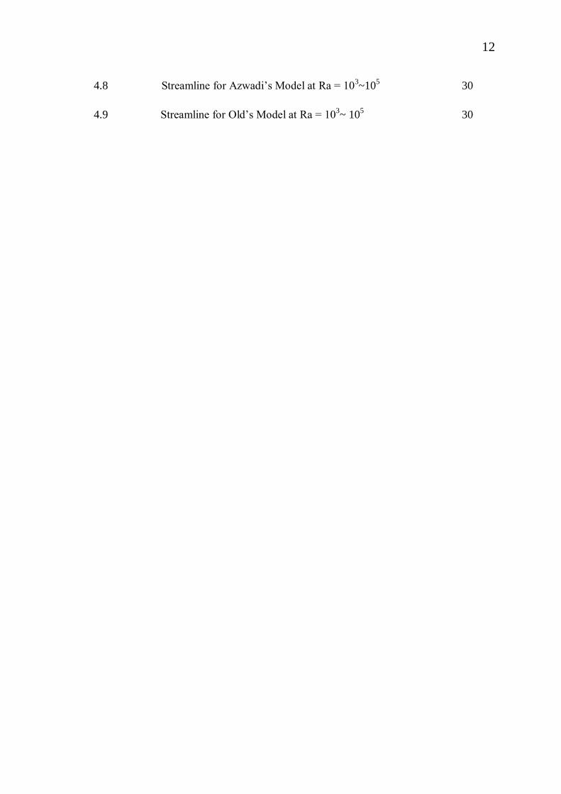
12

4.8 Streamline for Azwadi‟s Model at Ra = 103~10

5 30

4.9 Streamline for Old‟s Model at Ra = 103~ 10

5 30

13

LIST OF SYMBOLS

f:

c

Ω( f)

Density distribution function;

Microscopic velocity

Collision integral.

t Time

T

Ν

Α

β

Temperature

Kinematic viscosity

Thermal diffusivity

Thermal expansion coefficient

TC Cold temperature

TH Hot temperature

u Horizontal velocity

u Velocity vector

U Horizontal velocity of top plate

v Vertical velocity

V Volume

x Space vector

P Pressure

τ f ,g Time relaxation

υ Shear viscosity

β Thermal expansion coefficient

Ε

ν

α

μ

k

Internal energy

kinematic viscosity

thermal diffusivity

viscosity

thermal conductivity

ρ Density

Infinity temperature

Film temperature

Surface temperature

A Area of contact A

η Proportionally constant

χ Thermal diffusivity

Ω Collision operator

Average temperature

g Acceleration due to gravity

c Microscopic velocity

Equilibrium distribution function

f Distribution function

Pr Prandtl number

Ra Rayleigh number

Re Reynolds number

14

LIST OF ABBREVIATIONS

BGK Bhatnagar Gross krook

CFD Computational fluid dynamics

LBM Lattice Boltzmann method

LGA

D2Q4

D2Q9

Lattice gas approach

Two dimensional Four velocities model

Two dimensional Nine velocities model

LGCA Lattice gas cellular automata

PBC Periodic Boundary condition

PDEs Partial differential equations

15

CHAPTER 1

INTRODUCTION

1.1 INTRODUCTION

1.1.1 Navier-Stokes equations

The Navier–Stokes equations describe the motion of fluid substances that

is substances which can flow. These equations arise from applying Newton's

second law to fluid motion, together with the assumption that the fluid stress is the

sum of a diffusing viscous term (proportional to the gradient of velocity), plus a

pressure term. The mathematical relationship governing equation fluid flow is the

famous continuity equation and Navier Stokes equation given by. The Navier–

Stokes equations dictate not position but rather velocity. A solution of the Navier–

Stokes equations is called a velocity field or flow field, which is a description of

the velocity of the fluid at a given point in space and time. Once the velocity field

is solved for, other quantities of interest such as flow rate or drag force may be

found (X.He and L.S.Luo). Some exact solutions to the Navier–Stokes equations

exist. Examples of degenerate cases; with the non-linear terms in the Navier–

Stokes equations equal to zero; are Poisuelle flow, Couette flow and the oscillatory

Stokes boundary layer. But also more interesting examples, solutions to the full

non-linear equations, exist; for example the Taylor–Green vortex. Note that the

existence of these exact solutions does not imply they are stable: turbulence may

develop at higher Reynolds numbers.

16

1.1.2. Lattice Boltzmann Method (LBM)

Lattice Boltzmann methods (LBM) is a class of computational fluid

dynamics (CFD) methods for fluid simulation. Instead of solving the Navier–

Stokes equations, the discrete Lattice Boltzmann (LB) equation is solved to

simulate the flow of a Newtonian fluid with collision models such as Bhatnagar-

Gross-Krook (BGK). LB scheme is a scheme evolved from the improvement of

lattice gas automata and inherits some features from its precursor, the Lattice Gas

Automata (LGA).

The main motivation for the transition from LGA to LBM was the desire

to remove the statistical noise by replacing the Boolean particle number in a lattice

direction with its ensemble average, the so-called density distribution function.

Accompanying this replacement, the discrete collision rule is also replaced by a

continuous function known as the collision operator. In the LBM development, an

important simplification is to approximate the collision operator with the

Bhatnagar-Gross-Krook (BGK) relaxation term. This lattice BGK (LBGK) model

makes simulations more efficient and allows flexibility of the transport

coefficients.

Lattice Boltzmann models can be operated on a number of different

lattices, both cubic and triangular, and with or without rest particles in the discrete

distribution function. A popular way of classifying the different methods by lattice

is the DnQm scheme. Here "Dn" stands for "n dimensions" while "Qm" stands for

"m speeds". For example, D3Q15 is a three-dimensional Lattice Boltzmann model

on a cubic grid, with rest particles present.

Although LBM approach treats gases and liquids as systems consisting of

individual particles, the primary goal of this approach is to build a bridge between

the microscopic and macroscopic dynamics. It is by deriving macroscopic equations

from microscopic dynamics by means of statistic, rather than to solve macroscopic

equations.

17

1.2 PROBLEM BACKGROUND

The lattice Boltzmann method is an alternative approach to the finite difference,

finite element, and finite volume techniques for solving Navier-Stokes equations.

LB scheme is a scheme evolved from the improvement of lattice gas automata and

inherits some features from its precursor, the LGA. The implementation of the

Bhatnagar-Gross-Krook (BGK) approximation has been made for LB method to

improve its computational efficiency. The algorithm of LBM is simple, and easily

modified to allow for the application of other.

LBM originated from lattice gas automata (LGA) which is based on concepts

from the kinetic theory of gases. Two dimensional, four velocity model is one of the

most widely used today to modeling macroscopic flow phenomena. LGA views

fluids as arrays of discrete particles living on a discrete lattice, evolving some

interactive such as propagation and collision rules. Collision between the particles in

D2Q4 model will occur, and the change in velocity of each particle including its

performance will be found out.

1.2.1 Project Objective

To find out the performances for both types D2Q4 microscopic velocity

models.

1.2.2 Project Scopes

The scopes of this project are limited to D1Q4 microscopic velocity

model, at low Rayleigh number using heat transfer mechanism.

18

1.3 THESIS OUTLINE

The aim of this thesis is to study the methods of the lattice Boltzmann

equations in order to apply in two types of D2Q4 model in thermal fluid flow

problems. These methods utilize the statistical mechanics of simple discrete models

to simulate complex physical systems. The theory of lattice Boltzmann method in

nine and four velocity model are reviewed. Then the new concern here is in chapter

4. Two types of four velocity model are studied and will be evaluated at low

Rayleigh number heat transfer. The performance for both types D2Q4 microscopic

model is demonstrated in the simulations of porous thermal couette flow and natural

convection flow in a square cavity. Comparison of both models will be analyzed as

the final result.

In chapter 2, the isothermal fluid flows problem will be the main subject.

The concepts of distribution function are considered beside the theory of Boltzmann

equations. Then the derivations of Navier-Stokes equation from the Boltzmann

equations are also presented. Some simulation results are performed, to highlight the

important features of the isothermal LB model.

Then in chapter 3, the application of lattice Boltzmann scheme in thermal

fluid problem is investigated. By using the derivation of the discretised density

distribution function, a 4-velocity model is applied to develop the internal energy

distribution function. This model is validating to simulate the porous couette flow

problem for thermal fluid flow problems. The accuracy and stability analysis of the

model are discussed.

In chapter 4, the simulation of thermal fluids flow is applied to two

different types of four-velocity model. The same simulation test is performed for

both types and the accuracy and stability analysis of both models are also discussed.

These models are compared and tested to ensure its validity.

Finally in chapter 5, conclusions and discussion on future studies are

presented.

19

CHAPTER 2

LITERATURE STUDY

2.1 LATTICE BOLTZMANN METHOD

The lattice Boltzmann method is a powerful technique for the

computational modeling of a wide variety of complex fluid flow problems

including single and multiphase flow in complex geometries. It is a discrete

computational method based upon the Boltzmann equation. It considers a typical

volume element of fluid to be composed of a collection of particles that are

represented by a particle velocity distribution function for each fluid component at

each grid point (X.HE, 1997). The time is counted in discrete time steps and the

fluid particles can collide with each other as they move, possibly under applied

forces. The rules governing the collisions are designed such that the time-average

motion of the particles is consistent with the Navier-Stokes equation.

This method naturally accommodates a variety of boundary conditions

such as the pressure drop across the interface between two fluids and wetting

effects at a fluid-solid interface. It is an approach that bridges microscopic

phenomena with the continuum macroscopic equations. Further, it can model the

time evolution of systems. Lattice Boltzmann Method can be reviewed as a

numerical method to solve the Boltzmann equation. In LB method, the phase space

is discretized. In a LB model, the velocity of a particle can only be chosen from a

velocity set, which has only a finite number of velocities.

The Lattice Boltzmann Equation (LBE) method is described for

simulating micro- and meso-scale phenomena. The method is employed to study

multiphase and multicomponent flows in microchannels.

20

The primary goal of LBM is to build a bridge between the microscopic

and macroscopic dynamics rather than to dealt with macroscopic dynamics

directly. In other words, the goal is to derive macroscopic equations from

microscopic dynamics by means of statistics rather than to solve macroscopic

equation.

The Boltzmann equation for any lattice model is an equation for the time

evolution of fi (x,t), the single-particle distribution at lattice site x:

(2.1)

Statistical Mechanics

Density distribution function tf ,x

Moment of distribution

function

Macroscopic variables

Density, velocity, pressure, etc.

eqfftxftttcxf ),(),(

Figure 2.1: Lattice Boltzmann Theory (Rosdzimin, 2008)

21

2.2 COLLISION INTERGRAL, Ω( f )

Basic principle of LBM is including streaming step and collision step.

The particles move to another place in the variable direction with their velocities

(streaming step) and after they meet to each other, the collision happens (collision

step) and the particles will separate again. (streaming step) ( Xiaoyi et al ,1996).

We also can take an example from the „‟snooker‟. From this situation, means when

a ball hit to another ball, its can firstly streaming and then its will collision and it

become streaming again. Collisions between particles change their velocities, and

make them move in and out of the domain. A collision term describes the net

increase of the density of the number of particles in the domain due to the collision.

One of the simplest collision models is the Bhatnagar, Gross and Krook (BGK)

simplified collision model.

Boltzmann came out with the H-theorem where the value of distribution

function will always tend to the equilibrium distribution function, feq

during

collision process. The distribution function f can be relate to feq

.

2.3 BGK (BHATNAGAR, GROSS, AND KROOK)

n BGK model, the nonlinear collision term of the Boltzmann equation is

replaced by a simpler term and the model makes the derivation of the transport

equations for macroscopic variables much easier. A problem, which is easily

solved by the BGK model, is that of relaxation of a state of a fluid to equilibrium.

2.4 BOUNDARY CONDITION

The set of conditions specified for the behavior of the solution to a set of

differential equations at the boundary of its domain. Boundary conditions are

1, , , ,eqf x c t t t f x t f x t f x t

1 eqf f f(2.2)

(2.3

)

22

important in determining the mathematical solutions to many physical problems. In

a numerical simulation, it is impossible and unnecessary to simulate the whole

universe. Generally we choose a region of interest in which we conduct a

simulation. The interesting region has a certain boundary with the surrounding

environment. Numerical simulations also have to consider the physical processes in

the boundary region. In most cases, the boundary conditions are very important for

the simulation region's physical processes. Different boundary conditions may

cause quite different simulation results. Improper sets of boundary conditions may

introduce nonphysical influences on the simulation system, while a proper set of

boundary conditions can avoid that. So arranging the boundary conditions for

different problems becomes very important. While at the same time, different

variables in the environment may have different boundary conditions according to

certain physical problems. Commonly there are several different types of boundary

conditions.

2.4.1 Periodic boundary condition

Periodic boundary conditions (PBC) are a set of boundary conditions that

are often used to simulate a large system by modeling a small part that is far from

its edge. Periodic boundary conditions are particularly useful for simulating a part

of a bulk system with no surfaces present. Moreover, in simulations of planar

surfaces, it is very often useful to simulate two dimensions (e.g. x and y) with

periodic boundaries, while leaving the third (z) direction with different boundary

conditions, such as remaining vacuum to infinity. This setup is known as slab

boundary conditions.

Figure 2.2: Periodic Boundary Condition

Rigid Wall

Periodic

BC

Periodic

BC

Flexible

Wall

23

2.4.2 Bounce Back Boundary condition

The bounce-back boundary condition for lattice Boltzmann simulations is

evaluated for flow about an infinite periodic array of cylinders. The bounce-back

boundary condition is used to simulate boundaries of cylinders with both circular

and octagonal cross-sections. The convergences of the velocity and total drag

associated with this method are slightly sublinear with grid spacing. Error is also a

function of relaxation time, increasing exponentially for large relaxation times.

However, the accuracy does not exhibit a trend with Reynolds number between 0.1

and 100. The bounce-back boundary condition is shown to yield accurate lattice

Boltzmann simulations with reduced computational requirements for computational

grids of 170×170 or finer, a relaxation time less than 1.0 and any Reynolds number

from 0.1 to 100. For this range of parameters the root mean square error in velocity

and the relative error in drag coefficient are less than 1 % for the octagonal cylinder

and 2 % for the circular cylinder.

2.4 DISCRETIZATION OF MICROSCOPIC VELOCITY

For the discreatization of microscopic velocity, from the Gauss-Hermitte

integration, we can integrate from the continuous velocity to the 9-discrete velocity

and also 4-discrete velocity. We focused on the two type of discrete velocity [S.

Harris]. For the (poiseulle and couette flow) isothermal fluid flow, we are focusing

on 9-discrete velocity model and for the (porous couette flow) thermal fluid flow,

we are using 4-discrete velocity model.

24

2.5.1. Isothermal Fluid Flow

Figure 2.3: 9-Discrete Velocity Model

Figure 2.2 showed the 9-discrete velocity model that is going to be used

in simulation of isothermal fluid flow (poiseulle flow and coutte flow).

2.5.1.1 The Macroscopic Equation for Isothermal

By using chapmann-enskog expansion procedure, we can have the

navier-stroke equations accurate in continuity equations and in momentum

equation:

The relation between the time relaxation τ, in microscopic level and

viscosity of fluid ν, in macroscopic level is;

2

0

2 1

6P

t

2 1

6

(2.4)

(2.5)

(2.6)

25

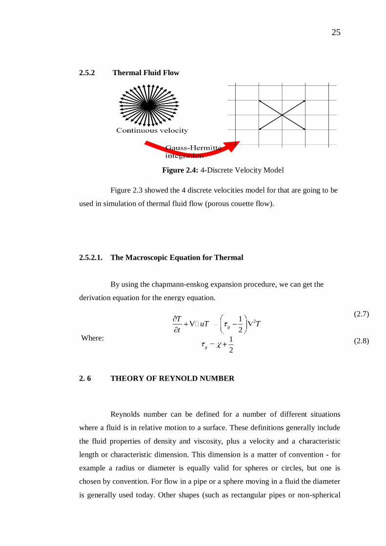
2.5.2 Thermal Fluid Flow

Figure 2.4: 4-Discrete Velocity Model

Figure 2.3 showed the 4 discrete velocities model for that are going to be

used in simulation of thermal fluid flow (porous couette flow).

2.5.2.1. The Macroscopic Equation for Thermal

By using the chapmann-enskog expansion procedure, we can get the

derivation equation for the energy equation.

Where:

2. 6 THEORY OF REYNOLD NUMBER

Reynolds number can be defined for a number of different situations

where a fluid is in relative motion to a surface. These definitions generally include

the fluid properties of density and viscosity, plus a velocity and a characteristic

length or characteristic dimension. This dimension is a matter of convention - for

example a radius or diameter is equally valid for spheres or circles, but one is

chosen by convention. For flow in a pipe or a sphere moving in a fluid the diameter

is generally used today. Other shapes (such as rectangular pipes or non-spherical

21

2g

TuT T

t

1

2g

(2.7)

(2.8)