Development of a stochastic convection schemesws00rsp/research/stochastic/seminar...Scale...

Development of a stochastic convectionscheme

R. J. Keane, R. S. Plant, N. E. Bowler, W. J. Tennant

Development of a stochastic convection scheme – p.1/45

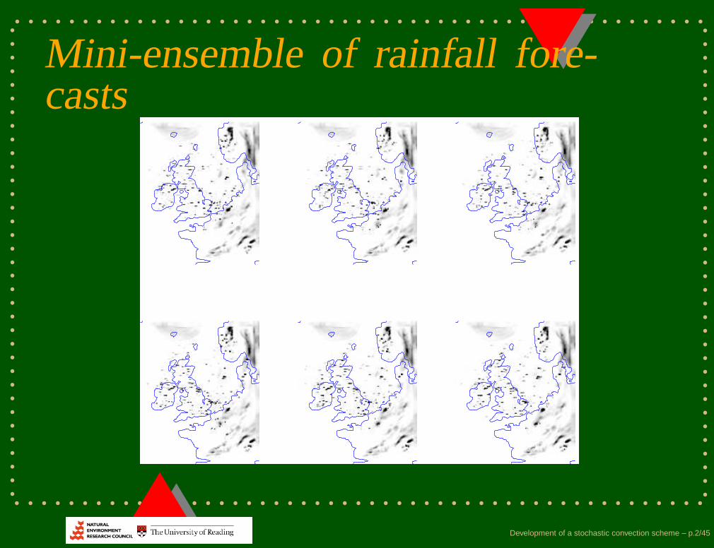
Mini-ensemble of rainfall fore-casts


Outline• Overview of stochastic parameterisation.• How the Plant Craig stochastic convective

parameterisation scheme works and the 3Didealised setup.

• Results: rainfall statistics.• A look at the Plant Craig scheme in a

mesoscale run.• Conclusions and future work.


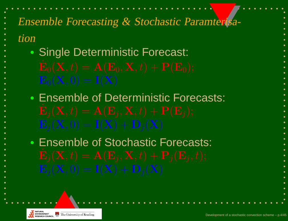
Ensemble Forecasting & Stochastic Paramterisa-

tion• Single Deterministic Forecast:

E0(X, t) = A(E0,X, t) + P(E0);E0(X, 0) = I(X)

• Ensemble of Deterministic Forecasts:Ej(X, t) = A(Ej,X, t) + P(Ej);Ej(X, 0) = I(X) + Dj(X)

• Ensemble of Stochastic Forecasts:Ej(X, t) = A(Ej,X, t) + Pj(Ej, t);Ej(X, 0) = I(X) + Dj(X)


How stochastic parameterisations may improve ensemble

forecasts: noise-induced drift


How stochastic parameterisations may improve ensemble

forecasts: better forecast of variability


Rank Histograms of surfacetemperature


Heavy Rain Devon and SouthWales 6th June 2009Ken Mylne, 4th SRNWP workshop on ShortRange Ensemble Prediction Systems, 2009.

© Crown copyright Met Office 4th SRNWP Workshop on short-range EPS, Exeter June 2009.

Heavy rain Devon & S. Wales Sat 6th June 2009

MOGREPS0600 5th June

ECMWF0000 5th June


Climate modelling of heavy pre-cipitationSun et. al. J. Clim. 2006


Conventional convective param-eterisationFor a constant large-scale situation, aconventional parameterisaion models theconvection independently of space:


Conventional convective param-eterisationThis leads to a uniform, mean value ofconvection whatever the grid box size:


Stochastic parameterisationA stochastic scheme allows the number andstrength of clouds to vary consistent with thelarge-scale situation:


Effect of ParamterisationOf course, this has no effect if the grid box islarge enough:


Stochastic ParameterisationBut for a smaller gridbox ...


Effect of ParamterisationThe scheme allows some convective variability:


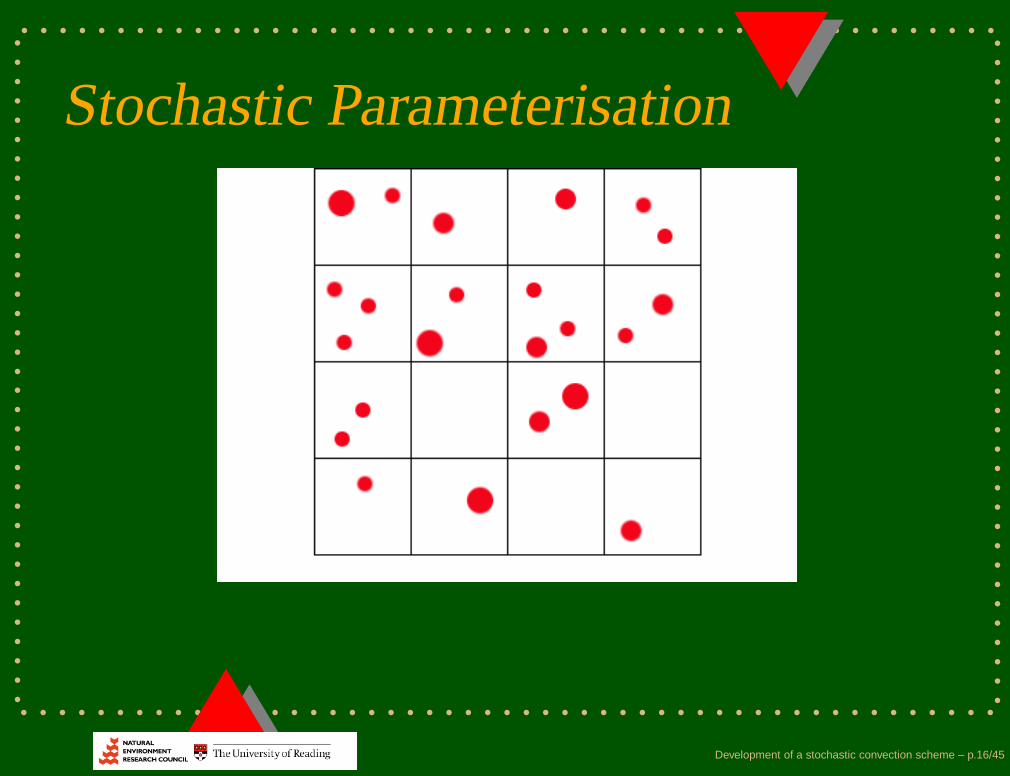
Stochastic Parameterisation


Effect of Paramterisation


The real worldThe distribution will be different in reality, but thevariability will be similar.


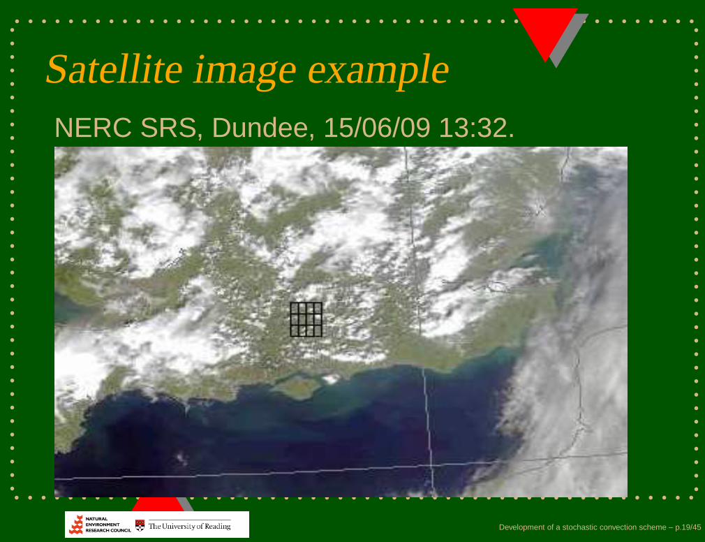
Satellite image exampleNERC SRS, Dundee, 15/06/09 13:32.


Scale separation: thermodynam-ics


Scale separation: rainfall


Convection parameterisationschemes

• Trigger function• Mass-flux plume model• Closure• Examples

• Gregory Rowntree (UM standard)• Kain Fritsch• Plant Craig (based on Kain Fritsch)


Plant Craig scheme: Analogies

Statistical Mechanics Convection

Particle Cloud

Energy per particle Mass flux per cloud m

Number of particles Number of clouds N

Ensemble average energy Ensemble average mass flux 〈M〉

Temperature Ensemble mean mass flux per cloud 〈m〉

Entropy Ensemble mean number of clouds 〈N〉


Plant Craig scheme: Methodol-ogy

• Obtain the large-scale state by averagingresolved flow variables over both space andtime.

• Obtain 〈M〉 from CAPE closure and definethe equilibrium distribution of m (Cohen-Craigtheory).

• Draw randomly from this distribution to obtaincumulus properties in each grid box.

• Compute tendencies of grid-scale variablesfrom the cumulus properties.


Plant Craig scheme: Averagingarea


Plant Craig scheme: ProbabilitydistributionAssuming a statistical equilibrium leads to anexponential distribution of mass fluxes per cloud:

p(m)dm =1

〈m〉exp

(

−m

〈m〉

)

dm.

So if m ∼ r2 then the probability of initiating aplume of radius r in a timestep dt is

〈M〉2r

〈m〉〈r2〉exp

(

−r2

〈r2〉

)

drdt

T.


Exponential distribution in aCRMCohen, PhD thesis (2001)


Ensemble Forecasting & Stochastic Paramterisa-

tion• Single Deterministic Forecast:

E0(X, t) = A(E0,X, t) + P(E0);E0(X, 0) = I(X)

• Ensemble of Deterministic Forecasts:Ej(X, t) = A(Ej,X, t) + P(Ej);Ej(X, 0) = I(X) + Dj(X)

• Ensemble of Stochastic Forecasts:Ej(X, t) = A(Ej,X, t) + Pj(Ej, t);Ej(X, 0) = I(X) + Dj(X)


PDF of total mass fluxAssuming that clouds are non-interacting, p(m)can be combined with a Poisson distribution forcloud number,

p(N) =〈N〉Ne−〈N〉

N !,

leading to the following distribution for total massflux:

p(M) =

(

〈N〉

〈m〉

)1/2

e−(〈N〉+M/〈m〉)M−1/2I1

(

2

√

〈N〉

〈m〉M

)

.


PDFs of mass flux in an SCM

• Plant & Craig, JAS, 2008


3D Idealised UM setup• Radiation is represented by a uniform cooling.• Convection, large scale precipitation and the

boundary layer are parameterised.• The domain is square, with bicyclic boundary

conditions.• The surface is flat and entirely ocean, with a

constant surface temperature imposed.• Targeted diffusion of moisture is applied.• The grid size is 32 km.


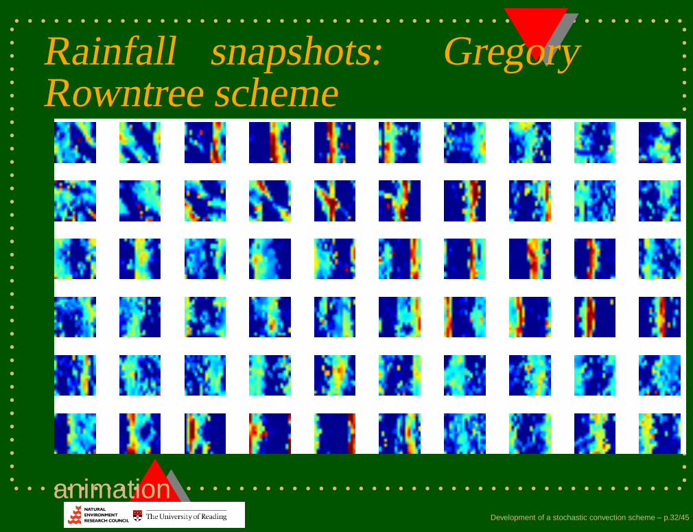
Rainfall snapshots: GregoryRowntree scheme

animationDevelopment of a stochastic convection scheme – p.32/45

Rainfall snapshots: Kain Fritschscheme


Rainfall snapshots: Plant Craigscheme


Model grid division16km 32km


PDFs ofm andM for maximumaveragingAveraging area: 480 km square.Averaging time: 1 hour.

0 0.2 0.4 0.6 0.8 1 1.2 1.4 1.6 1.8 2

x 108

−25

−24

−23

−22

−21

−20

−19

−18

−17

m (kg s−1)

ln (

p(m

) (k

g−

1s)

)

schemetheory

0 1 2 3 4 5 6

x 108

0

1

2

3

4

5

6x 10

−9

M (kg s−1)

p(M

) (k

g−

1 s

)

schemetheory


PDFs ofm andM for no averag-ing

0 0.2 0.4 0.6 0.8 1 1.2 1.4 1.6 1.8 2

x 108

−25

−24

−23

−22

−21

−20

−19

−18

−17

m (kg s−1)

ln (

p(m

) (k

g−

1s)

)

schemetheory

0 1 2 3 4 5 6 7 8

x 108

0

1

2

3

4

5

6

7x 10

−9

M (kg s−1)

p(M

) (k

g−

1 s

)

schemetheory


PDFs ofm andM for intermedi-ate averagingAveraging area: 160 km square.Averaging time: 1 hour.

0 0.2 0.4 0.6 0.8 1 1.2 1.4 1.6 1.8 2

x 108

−26

−25

−24

−23

−22

−21

−20

−19

−18

−17

m (kg s−1)

ln (

p(m

) (k

g−

1s)

)

schemetheory

0 1 2 3 4 5 6

x 108

0

1

2

3

4

5

6

7x 10

−9

M (kg s−1)

p(M

) (k

g−

1 s

)

schemetheory


PDFs ofm andM for 16 km (noaveraging)

0 0.2 0.4 0.6 0.8 1 1.2 1.4 1.6 1.8 2

x 108

−25

−24

−23

−22

−21

−20

−19

−18

−17

m (kg s−1)

ln (

p(m

) (k

g−

1s)

)

schemetheory

0 0.5 1 1.5 2 2.5 3 3.5 4

x 108

0

1

2

3

4

5

6

7x 10

−9

M (kg s−1)

p(M

) (k

g−

1 s

)

schemetheory


PDFs ofm andM for 16 km (in-termediate averaging)

0 0.2 0.4 0.6 0.8 1 1.2 1.4 1.6 1.8 2

x 108

−25

−24

−23

−22

−21

−20

−19

−18

−17

m (kg s−1)

ln (

p(m

) (k

g−

1s)

)

schemetheory

0 0.5 1 1.5 2 2.5 3 3.5 4

x 108

0

1

2

3

4

5

6

7x 10

−9

M (kg s−1)

p(M

) (k

g−

1 s

)

schemetheory


Case study: CSIP IOP18• Starts at 25th August 2005, 07:00.• 12 km grid with 146 × 182 grid points.

20 40 60 80 100 120

20

40

60

80

100

120

140

160

180

0

0.1

0.2

0.3

0.4

0.5

0.6

0.7

0.8

0.9

1x 10

−3


Ensemble of 6 runs using PCscheme

20 40 60 80100120

50

100

150

20 40 60 80100120

50

100

150

20 40 60 80100120

50

100

150

20 40 60 80100120

50

100

150

20 40 60 80100120

50

100

150

20 40 60 80100120

50

100

150


Rainfall against time for each ofthree schemes

8 10 12 14 16 18 200

0.05

0.1

0.15

0.2

0.25

0.3

0.35

mea

n ra

infa

ll (kg

m−2

)

time (hours)

PC cvPC lsPC totGR cvGR lsGR totKF cvKF lsKF tot


Future work• Implement the PC scheme in MOGREPS, to

determine its impact on variability.• Run on NAE domain (∼ 20 km), for one

Summer month.• Compare with existing GR run and

deterministic version of PC.• Look at the effect of the scheme, and its

stochastic nature, on the variability of theensemble and the spread-error relationship.


Conclusions• The convective variability in the scheme is according to

the Cohen Craig theory, and is not due to spuriousnoise from the large-scale.

• An averaging area of roughly 160 km is required toeffect this.

• The statistical behaviour of the scheme is correct atdifferent resolutions, although the amount of averagingrequired may vary.

• The scheme behaves sensibly in a mesoscale setup,and is ready to be implemented in an ensembleprediction system.


Development of a stochastic convection schemesws00rsp/research/stochastic/seminar...Scale...

Documents

Transcript of Development of a stochastic convection schemesws00rsp/research/stochastic/seminar...Scale...