Development and Evaluation of a Simple Algorithm to Find ...
10
46 The Open Atmospheric Science Journal, 2008, 2, 46-55 1874-2823/08 2008 Bentham Science Publishers Ltd. Development and Evaluation of a Simple Algorithm to Find Cloud Optical Depth with Emphasis on Thin Ice Clouds J.C. Barnard *,a , C.N. Long a , E.I. Kassianov a , S.A. McFarlane a , J.M. Comstock a , M. Freer b and G.M. McFarquhar b a Pacific Northwest National Laboratory, Richland, Washington, USA b University of Illinois at Urbana-Champaign, Urbana, Illinois, USA Abstract: An algorithm is presented here for determining cloud optical depth, , using data from shortwave broadband ir- radiances, focusing on the case of optically thin clouds. This method is empirical and consists of a one-line equation. This method is applied to cirrus clouds observed at the Atmospheric Radiation Measurement Program Climate Research Facil- ity (ACRF) at Darwin, Australia, during the Tropical Warm Pool International Cloud Experiment (TWP-ICE) campaign and cirrus clouds observed at the ACRF Southern Great Plains (SGP) site. These cases were chosen because independent verification of cloud optical depth retrievals was possible. For the TWP-ICE case, the calculated optical depths agree to within 1 unit with calculated from a vertical profile of ice particle size distributions obtained from an aircraft sounding. For the SGP case, the results from the algorithm correspond reasonably well with values obtained from an average over other retrieval methods, some of which have been subject to independent verification. The medians of the two time series are 0.79 and 0.81, for the empirical and averaged values, respectively. Because such close agreement is likely to be fortui- tous and therefore not truly represent the performance of our method, values derived from our method were compared to values obtained from lidar data. Over a three year period, the difference in median values between the two methods is about 0.6, with the lidar optical depths being larger. This tool may be applied wherever measurements of the direct, dif- fuse, and total components of the shortwave broadband flux are available at 1- to 5-minute resolution. Because these measurements are made across the world, it then becomes possible to estimate optical depth for both liquid water and ice clouds at many locations. Keywords: Cloud, optical depth, algorithm. 1. INTRODUCTION Optically thin clouds are now an important topic in the climate community because of their ubiquity and effect on radiative fluxes. The defining feature of such clouds is their low water (ice) path and correspondingly low optical depth. Accurate determination of these and other cloud properties is critical for their representation in climate models, but the “thinness” of these clouds makes it difficult to determine their microphysical and optical properties, particularly using remote sensing [1]. Remote sensing of cloud visible optical depth, , is possi- ble using measurements from a variety of instruments along with their respective retrieval algorithms, as described in Turner et al. [1] for thin liquid water clouds, and Comstock et al. [2] for ice clouds. To this myriad mix of algorithms, we present here yet another algorithm that uses data from broadband radiometers to find . This method is simple to use and requires minimal amounts of computer time. Con- sidering these factors and the relative abundance of broadband irradiance measurements compared to more so- phisticated and expensive instruments, the algorithm may be used to easily estimate thin cloud properties at many loca- tions worldwide. *Address correspondence to this author at the Pacific Northwest National Laboratory, Richland, Washington, USA; E-mail: [email protected] In a previous paper [3], abbreviated henceforth as BL, we described the development of the algorithm as applied to optically thick water clouds. Here we derive a more elegant and physically based formulation. Although this new formu- lation is strictly speaking valid only for thick clouds, we ap- ply the method to the optically thin case in hopes that it works reasonably well in comparison to other, more sophis- ticated algorithms. Such hopes are borne out, as described below. 2. ALGORITHM DEVELOPMENT AND ALGORITHM ERRORS 2.1. Algorithm Development The original algorithm described in BL is entirely em- pirical and uses broadband irradiances to find . In prepara- tion for the derivation of the more physically based algo- rithm used in this paper, we briefly summarize the empirical derivation presented in BL. The basic underpinning of the empirical formula presented in BL is that, for a horizontally homogenous, optically thick cloud deck, , should be a func- tion of the diffuse irradiance transmission and the cosine of the solar zenith angle, μ 0 . The diffuse transmission is defined here as D/C, where D is the measured diffuse irradiance and C is the clear sky total shortwave irradiance, the shortwave irradiance that would be measured in the absence of clouds. This quantity is found easily using the shortwave flux analy- sis described in [4] and has been used in rigorous broadband
Transcript of Development and Evaluation of a Simple Algorithm to Find ...
46 The Open Atmospheric Science Journal, 2008, 2, 46-55
1874-2823/08 2008 Bentham Science Publishers Ltd.
Development and Evaluation of a Simple Algorithm to Find Cloud Optical Depth with Emphasis on Thin Ice Clouds
J.C. Barnard*,a
, C.N. Longa, E.I. Kassianov
a, S.A. McFarlane
a, J.M. Comstock
a, M. Freer
b and
G.M. McFarquharb
aPacific Northwest National Laboratory, Richland, Washington, USA
bUniversity of Illinois at Urbana-Champaign, Urbana, Illinois, USA
Abstract: An algorithm is presented here for determining cloud optical depth, , using data from shortwave broadband ir-
radiances, focusing on the case of optically thin clouds. This method is empirical and consists of a one-line equation. This
method is applied to cirrus clouds observed at the Atmospheric Radiation Measurement Program Climate Research Facil-
ity (ACRF) at Darwin, Australia, during the Tropical Warm Pool International Cloud Experiment (TWP-ICE) campaign
and cirrus clouds observed at the ACRF Southern Great Plains (SGP) site. These cases were chosen because independent
verification of cloud optical depth retrievals was possible. For the TWP-ICE case, the calculated optical depths agree to
within 1 unit with calculated from a vertical profile of ice particle size distributions obtained from an aircraft sounding.
For the SGP case, the results from the algorithm correspond reasonably well with values obtained from an average over
other retrieval methods, some of which have been subject to independent verification. The medians of the two time series
are 0.79 and 0.81, for the empirical and averaged values, respectively. Because such close agreement is likely to be fortui-
tous and therefore not truly represent the performance of our method, values derived from our method were compared to
values obtained from lidar data. Over a three year period, the difference in median values between the two methods is
about 0.6, with the lidar optical depths being larger. This tool may be applied wherever measurements of the direct, dif-
fuse, and total components of the shortwave broadband flux are available at 1- to 5-minute resolution. Because these
measurements are made across the world, it then becomes possible to estimate optical depth for both liquid water and ice
clouds at many locations.
Keywords: Cloud, optical depth, algorithm.
1. INTRODUCTION
Optically thin clouds are now an important topic in the
climate community because of their ubiquity and effect on
radiative fluxes. The defining feature of such clouds is their
low water (ice) path and correspondingly low optical depth.
Accurate determination of these and other cloud properties is
critical for their representation in climate models, but the
“thinness” of these clouds makes it difficult to determine
their microphysical and optical properties, particularly using
remote sensing [1].
Remote sensing of cloud visible optical depth, , is possi-
ble using measurements from a variety of instruments along
with their respective retrieval algorithms, as described in
Turner et al. [1] for thin liquid water clouds, and Comstock
et al. [2] for ice clouds. To this myriad mix of algorithms,
we present here yet another algorithm that uses data from
broadband radiometers to find . This method is simple to
use and requires minimal amounts of computer time. Con-
sidering these factors and the relative abundance of
broadband irradiance measurements compared to more so-
phisticated and expensive instruments, the algorithm may be
used to easily estimate thin cloud properties at many loca-
tions worldwide.
*Address correspondence to this author at the Pacific Northwest National
Laboratory, Richland, Washington, USA; E-mail: [email protected]
In a previous paper [3], abbreviated henceforth as BL, we
described the development of the algorithm as applied to
optically thick water clouds. Here we derive a more elegant
and physically based formulation. Although this new formu-
lation is strictly speaking valid only for thick clouds, we ap-
ply the method to the optically thin case in hopes that it
works reasonably well in comparison to other, more sophis-
ticated algorithms. Such hopes are borne out, as described
below.
2. ALGORITHM DEVELOPMENT AND ALGORITHM ERRORS
2.1. Algorithm Development
The original algorithm described in BL is entirely em-
pirical and uses broadband irradiances to find . In prepara-
tion for the derivation of the more physically based algo-
rithm used in this paper, we briefly summarize the empirical
derivation presented in BL. The basic underpinning of the
empirical formula presented in BL is that, for a horizontally
homogenous, optically thick cloud deck, , should be a func-
tion of the diffuse irradiance transmission and the cosine of
the solar zenith angle, μ0. The diffuse transmission is defined
here as D/C, where D is the measured diffuse irradiance and
C is the clear sky total shortwave irradiance, the shortwave
irradiance that would be measured in the absence of clouds.
This quantity is found easily using the shortwave flux analy-
sis described in [4] and has been used in rigorous broadband

Simple Algorithm to Find Cloud Optical Depth The Open Atmospheric Science Journal, 2008, Volume 2 47
algorithms, which use detailed radiative transfer calculations
to find [5]. In the original formulation, we postulated that
0( / )empirical f D Cμ= , (1)
where empirical is an empirical representation of , is an
exponent, to be determined, and f is a functional form, also
to be determined. We found by first plotting versus the
variable, r = D/(Cμ0 ), for a given value of . Then using a
trial-and-error procedure was adjusted repeatedly to
achieve the best possible “collapse” of the values on a sin-
gle curve so that was, to the extent possible, a single valued
function of r.
This procedure requires values and these were gener-
ated using the algorithm of Min and Harrison [6], which cal-
culates for optically thick ( 5), plane parallel, liquid wa-
ter clouds using diffuse irradiance data from the Multi-Filter
Rotating Shadowband Radiometer (MFRSR) [7]. The result
of this procedure is shown in Fig. (1) (similar to Fig. (1) in
BL). This plot shows Log[ ], where is calculated using the
Min and Harrison algorithm, plotted versus r. The irradiance
data
0 0.2 0.4 0.6 0.8 1
r ( = T/(Cμ01/4))
0
1
2
3
4
5
6
7
Lo
ge
[];
f
rom
Min
alg
ori
thm
Barrow
Manus Island
SGP (Sites E13 and E22)
F1, initial empirical fit
F2 = (1.16/r-1)/((1-A)(1-g))
Fig. (1). Equation (9) as fitted to cloud optical depth calculations.
This figure also shows the function F1, the initial empirical fit from BL.
required to determine were obtained from the ACRF site in
Barrow, Alaska, the ACRF Tropical Western Pacific (TWP)
Manus Island site, and two ACRF SGP sites. The number of
points used in this analysis, representing 5-min averages of r
and over the year 2000, ranges from about 6700 at Barrow
to about 9100 for the two SGP sites. To remove the effect of
broken cloudiness that acutely violates the plane parallel
assumption required by the Min algorithm, we only consid-
ered cases in which the fractional sky cover, as determined
by applying the Long algorithm [8] to broadband irradiances,
was greater than 0.99. The plot shows the best “collapse” of
the data which occurs when the exponent was chosen to be
. Further justification for this choice of exponent will be
provided below. A hyperbolic arctangent was chosen as the
function f in Eq. (1), and this function is shown in Fig. (1).
We denote this particular function f as F1.
In contrast to this completely empirical approach, our
new algorithm is partially based on the physics of radiative
transfer, and can therefore be described as semi-empirical.
The derivation of the new algorithm begins with the Edding-
ton approximation described by Shettle and Weinman [9]. In
this approximation, the total irradiance, T, at the Earth’s sur-
face is:
( )
( )
( )
0 0
0
0
02 3 1 3(1 )(1 )
(4 3(1 )(1 )
T F
e e A g
eA g
μ μ
μ
μ
μ
=
+
++
, (2)
where F (W/m2) is an extraterrestrial irradiance; A, is the
broadband surface albedo; and g is the cloud droplet or ice
particle asymmetry factor. For our derivation, we assume
that clouds are the only agents that act on the solar radiation,
and that there is no cloud absorption. As noted by Hu and
Stamnes [10] this latter assumption is good for the visible
region of the solar spectrum. For large /μ0 ( 5 ), T be-
comes
( )( )
( )0 02 3
4 3(1 )(1 )T F
A g
μ μ+=
+. (3)
We now re-define the parameter, r, as
0
TrCμ
= , (4)
where T (W/m2) is the measured total irradiance. Note that
we now use the measured total irradiance, T, whereas the old
algorithm used the measured diffuse irradiance, D. As noted
in Long and Ackerman [4], the diurnal variation of C is most
dependent on μ0; this dependence is well-represented by the
empirical fit, C = Bμ01.25
, where B (W/m2) is a fitting con-
stant. The variable r is therefore
( ) ( )
( )0 0
1.25
0 0
2 3
4 3(1 )(1 )
Fr
B A g
μ μ
μ μ
+=
+. (5)
The numerator μ0(2 + 3μ0) is approximated extremely
well by 5μ01.51
and making this substitution yields
( )
( )
( )
( )
1.51
0
1.25
0 0
1.51
0
1.25
0 0
5
4 3(1 )(1 )
5
4 3(1 )(1 )
r
F
B A g
F
B A g
μ
μ μ
μ
μ μ
=
+
=+
. (6)
Taking = effectively removes the dependence on the
solar zenith angle on the right hand side of Eq. (6). Solving
for gives

48 The Open Atmospheric Science Journal, 2008, Volume 2 Barnard et al.
4 51
3 4
(1 )(1 )
FB
r
A g= , (7)
which suggests an empirical relationship of the form
1 1
(1 )(1 )
c
r
A g= , (8)
where c1 is a fitting constant. This constant is determined by
trial and error: it is adjusted until the best fit between the
optical depth from the Min algorithm and the empirical
equation, Eq. (8), is achieved. The best fit, assessed visually,
is given with c1 1.16 and the expression for the empirical
optical depth, empirical, is therefore
2
1.161
( )(1 )(1 )
empirical
rF r
A g= = = . (9)
This equation, denoted as F2(r), is also shown in Fig. (1),
where it is seen that F1(r), the hyperbolic arctangent, and
F2(r) are nearly identical. Therefore the application of Eq.
(9) to optically thick liquid water clouds should produce the
same values of empirical as discussed in BL, and we will not
discuss the case of optically thick clouds here. Rather we
focus on optically thin ice clouds.
2.2. Errors
The parameter r = (T/C)/μ0 in Eq. (9) is proportional to
the atmospheric transmission (T/C) throughout the entire
atmospheric column that includes clouds and clear air. Using
this definition, the transmission is defined with respect to the
clear sky irradiance, C, rather than the top of atmosphere
irradiance. (Note also that because T and C are obtained from
the same set of instruments, calibration errors cancel in the
ratio.) For the cloudy skies of interest, C is an estimate of the
hypothetical clear sky irradiance, defined as the irradiance
that would be measured in the absence of the clouds. Using
C to define transmission tends to reduce retrieval errors be-
cause factors that affect transmission in the clear air above
and below the clouds are approximately accounted for.
These factors include aerosol optical depth, aer; abun-
dances of water vapor and ozone, and surface pressure.
Quantitative error estimates caused by variations in these
factors are provided in BL. Here we briefly explain why the
errors associated with these factors tend to be small. The
clear sky irradiance, C, is found by the realization that the
surface solar fluxes are most influenced by μ0, and accord-
ingly, C is assumed to have the form C Bμ0b, where B and
b are fitting parameters. These parameters are chosen to
minimize the difference between Bμ0b and the measured
clear sky, total downwelling shortwave irradiance during the
day. This procedure finds a B and b for each clear day in a
long time series of irradiance data; typically b is about 1.25
while B is about 1100 W/m2. For days that do not meet the
clear sky criterion, interpolation of the parameters B and b
for clear days on either side of the day in question is used.
The resulting estimate for the clear sky total downwelling
irradiance therefore contains some information about the
background aerosol, water vapor abundances, and variations
in surface pressure. Long and Ackerman [4] tested this pro-
cedure by examining the irradiances calculated for a clear
day using B and b interpolated from other clear days before
and after this day. They found that the root mean square er-
ror of the “interpolated” irradiances versus the measurements
was about 13 W/m2, within the measurement error of total
irradiance. This suggests that, in most cases, variations in
aer, water vapor, and surface pressure will be mostly ac-
counted for in the calculation of the transmission, because
the value of C for the day in question is likely to be a good
estimate of the true, clear sky surface irradiance. Rare excep-
tions to this conclusion would occur, for example, during
pollution events with very large values of aer, far outside the
typical range. Such atypically large values would not be cap-
tured by the procedure described above.
Cloud properties such as effective particle radius and
particle shape affect our results. In the old formulation given
in BL, these properties were not explicitly taken into ac-
count. By contrast, in the new method these factors are ap-
proximately dealt with in the choice of g in Eq. (9); this will
be discussed in section 4. To avoid problems associated with
mixed phase clouds, we focus exclusively on ice clouds in
this study. These clouds occur at very large altitudes with
correspondingly cold temperatures so that liquid water can-
not exist. To avoid the problem of broken cloud scenes, we
use the algorithm of Long et al. [8] to identify cases when
the fractional sky cover is greater than 0.9. Even in the pres-
ence of fractional sky covers in excess of 0.9, the clouds will
not likely be horizontally and vertically homogenous. In this
regard, the optical depth so retrieved should be considered an
“effective” optical depth, meaning that it is some average
over the clouds within the field of view of the instruments
measuring the shortwave irradiances.
Because the focus here is on thin ice clouds we cannot
overemphasize that Eq. (9) was derived for the optically
thick case (defined here as > 5), and there is no rigorous
physical reason to expect it to work for the thin cloud case.
Indeed, in the asymptotic limit of clear skies, such that T
C, Eq. (9) yields empirical values between about -1.4 to about
1.0, depending upon the solar zenith angle, although the av-
eraged value of for 0.2 μ0 1.0 is virtually zero. (The
value of μ0 at which empirical equals zero is about 0.55.) Cog-
nizant of these problems, we nonetheless apply the algorithm
to the thin cloud case, and we find that it works surprisingly
well vis-à-vis other methods, particularly when finding dis-
tributions of optical depth. Given that at the present time the
uncertainties associated with other retrieval methods are not
well known, we think this method would be an excellent
choice for predicting “effective” optical depth distributions
over a wide range of optical depth.
3. PHILOSOPHICAL CONSIDERATIONS: ALGO-RITHM VALIDATION
Algorithm validation is only credible when the quantity
retrieved by the algorithm can be verified in an independent

Simple Algorithm to Find Cloud Optical Depth The Open Atmospheric Science Journal, 2008, Volume 2 49
manner. For cloud optical depth, this independent verifica-
tion can be done in several ways, none of which is perfect.
We mention two methods here. The first of these consists of
deriving an optical depth based on in situ cloud measure-
ments of particle size distributions and, in the case of ice
clouds, ice particle shape. Obviously, an optical depth de-
termined in this manner is completely independent from
ground-based retrievals of , and a comparison between the
two provides some information of how well the retrieval
algorithm works. The second method is termed “radiative
flux closure”. With this scheme, retrieved cloud properties
such as , asymmetry parameter, g, and single scattering al-
bedo, 0, are fed to a radiative transfer model to calculate
surface fluxes. The extent to which calculated and measured
fluxes agree is used to evaluate the retrieval algorithm.
3.1. Algorithm Validation Using a “First Principles” Cloud Optical Depth
Goody and Yang [11] define the optical path as the inte-
gral of extinction between two points, A and B, as
int
,
int
optical path ( )
po A
v
po B
e s ds= , (10)
where ev, is the volume extinction coefficient with units
(1/length), as a function of wavelength, ; and ds is an ele-
ment of path length between point A and point B. The “nor-
mal” optical depth [12] of the cloud is the optical path found
on a vertical line between the top and bottom of the cloud.
We use this as our definition of cloud optical depth, and give
it the label fp, where the subscript “fp” stands for “first prin-
ciples”. Of course, fp is a function of , but in the visible
spectral region, it is not expected to vary significantly over
wavelength [10] because ice crystals with radii between 10
and 1000 μm have size parameters (x = 2 r/ ) between 125
(21) and 12500 (2100) for = 0.5 (3.0 μm), suggesting geo-
metric optics with an extinction coefficient of 2 applies over
this spectral region.
In practice it is not possible to find fp exactly, because
the measurements needed to find fp are subject to significant
uncertainties. Here we estimate it using the profile of extinc-
tion between cloud top and cloud bottom. This profile can be
determined from aircraft measurements of cloud particle size
distribution, and cloud particle shape and phase throughout
the depth of a cloud, although both horizontal inhomogene-
ities, and uncertainties and approximations in the observa-
tions complicate the analysis [13,14]. Once the size distribu-
tion, shape, and phase are known, Mie theory, or other com-
putation techniques for non-spherical particles (e.g., ray trac-
ing), can be applied to find ev, (z). Integration over the depth
of the cloud yields an estimate of fp. To explicitly distin-
guish between the idealized, “first principle” optical depth
and its estimate, we assign the symbol est to this quantity.
When using in situ cloud measurements for the evalua-
tion of algorithms, one must be mindful of the many consid-
erations summarized by Comstock et al. [2]. These include:
collocation errors and sampling volume inconsistencies be-
tween the aircraft and the ground-based instruments, particle
breakup [14] and other instrumental errors, and the inevitable
inexactness of converting the measured data to extinction
values caused, for example, by using idealized particle
shapes to calculate extinction.
3.2. Flux Closure Validation
For completely clear skies, flux closure studies have been
remarkably successful in achieving consistency between
aerosol optical properties and surface broadband fluxes.
Michalsky et al. [15] report that biases between measured
and model flux are less than 2% for direct and diffuse com-
ponents. On the other hand, broadband flux closure for the
cloudy case is much more difficult because of the problem of
determining cloud optical properties throughout the volume
of atmosphere sensed by the surface radiometers and the
concomitant potential of 3-D radiative transfer effects. Mind-
ful of these problems, Turner et al. [1] and Comstock et al.
[2] describe radiative flux closure efforts to assess the valid-
ity of retrieved values of . In short, their flux closure
schemes follow these steps: (1) take the retrieved value of ,
and either assumed (or measured) optical properties of the
cloud particles, (2) plug these values into a radiative transfer
model, (3) calculate surface fluxes, and (4) compare calcu-
lated and observed surface fluxes. This scheme is followed
approximately in [2] to show the relationship between re-
trieved values used to calculate surface fluxes and meas-
ured surface fluxes. They assumed that the ice particles pos-
sessed scattering properties of bullet-rosette crystals, and
found that on a qualitative basis, measured and observed
fluxes tracked each other reasonably well. Quantitative
agreement was not nearly as good as for clear sky closure
cases, illustrating the challenges associated with radiative
flux closure in the presence of clouds.
4. ALGORITHM EVALUATION
4.1. Evaluation Test Cases
As noted above we choose data sets that permitted either
a direct, independent determination of to be made, or that
provided another means of independent verification, such as
a radiative flux closure. The data sets used are listed in Table
1. The first data case, chosen to evaluate the algorithm under
conditions of thin tropical cirrus, uses data from the ACRF
TWP Darwin site, located in the northern coast of Australia.
The data were obtained during the TWP-ICE campaign (http:
//acrf-campaign.arm.gov/twpice/) that took place during
early 2006. For several days during the campaign the Scaled
Composites Proteus aircraft (http: //www.arm.gov/about/
020206release.stm) executed spiral ascents and descents
through the cloud layers allowing est to be found. The sec-
ond data set was chosen to evaluate the algorithm for mid-
latitude cirrus clouds. This data set was taken during the
ARM Program’s cloud intensive operational period (IOP)
that took place during March 2000. A particular advantage of
using this data set is that it has already been a subject of in-
tense analysis of cloud optical depth retrieval algorithms [2],
and this analysis includes an independent verification of the
retrievals.

50 The Open Atmospheric Science Journal, 2008, Volume 2 Barnard et al.
During both of these campaigns, measurements were
made of the total, direct, and diffuse components of the
shortwave broadband irradiance using the usual suite of in-
struments: an Eppley Normal Incidence Pryheliometer
(NIP) to measure the direct beam irradiances, and either an
Eppley 8-48 Black & White pyranometer (TWP-ICE) or an
Eppley Precision Spectral Pyranometer (PSP, ARM Cloud
IOP) to measure the diffuse irradiance. The PSP measure-
ments were corrected for thermal offsets using the method of
Younkin and Long [16]. Our algorithm requires as input the
total irradiance, and for this quantity, we take the sum of the
diffuse irradiance plus the direct beam irradiance multiplied
by μ0.
The MFRSR was also operational during these cam-
paigns. The MFRSR measures the diffuse, direct, and total
components of the irradiances at six discrete wavelengths:
415, 500, 615, 673, and 870 nm. We use the direct compo-
nent of the irradiance at 415 nm to find using an algorithm
similar in spirit to [17], in which apparent cloud optical
depths obtained directly from the Beer-Lambert law are cor-
rected by removing the effect of diffuse light scattered into
the field of view of the detector (3.3°) by large cloud parti-
cles. The total optical depth derived directly from MFRSR
data is total = Rayleigh + aer + cloud,apparent, assuming no gase-
ous absorption, where Rayleigh is the Rayleigh component.
Subtracting this component and aer from total leaves the
apparent cloud optical depth, cloud,apparent. This is an underes-
timate of the actual cloud optical depth because of the non-
negligible amount of forward scattering mentioned above.
Using Monte Carlo calculations the forward scattering
contribution to the apparent cloud optical depth can be ac-
counted for. The magnitude of this correction depends on the
actual cloud optical depth, the size distribution, and cloud
particle single scattering albedo. For the size distribution, we
use that derived from TWP-ICE data, described in section.
4.2. Min et al. [17] suggest that the forward scattering cor-
rections are not that sensitive to variations in the ice particle
phase function, and this implies that the corrections derived
using the TWP-ICE size distribution would be valid for other
cases. Single scattering albedo was taken as a 1.0, because at
415 nm cloud particles do not absorb. From these calcula-
tions, we found that the correction to cloud,apparent was very
simple: for the solar zenith angles considered here, and for a
wavelength of 415 nm, the correction for ice clouds amounts
to multiplying cloud,apparent by 1.9. When appropriate, we will
show these optical depths, DB ( = 1.9 cloud,apparent), termed
“direct beam” (DB), as an aid for the evaluation of our algo-
rithm.
4.2. TWP-ICE
We present results obtained from our algorithm for the
day 25 January 2006, during the hours 1500 through 1700
LST, for this site LST = UTC + 9.5. During this period, the
high, thin cirrus was relatively uniform across the sky as
shown from the image depicted in Fig. (2), taken from the
Total Sky Imager (http: //www.arm.gov/instruments). The
Fig. (2). Total sky imager snapshot taken at about 1600 LST, Janu-
ary 25, 2006, during the TWP-ICE campaign. The cirrus clouds in
this scene are relatively optically thick. The fractional sky cover for this scene, from the routine of Long et al. [8], is 0.94.
cloud sky cover was greater than 0.9 for the entire time pe-
riod indicating that clouds filled the sky. This is essential
because the plane-parallel assumption behind our simple
algorithm is better satisfied than for more broken cloud
scenes. During this day, at approximately 1650 LST, the
Scaled Composites Proteus aircraft spiraled down through a
cirrus cloud directly above the ACRF Darwin site, and
measurements were made of the ice crystal shapes by the
Stratton Park Engineering Company’s (SPEC Inc.) Cloud
Particle Imager (CPI), and of the ice crystal size distributions
by Droplet Measurement Technology’s (DMT) Cloud and
Aerosol Spectrometer (CAPS) and the Cloud Imaging Probe
Table 1. Data Sets Used for Algorithm Verification
Name Location (Site, Latitude, Longitude) Time Period of Campaign Range of μ0
TWP-ICE Darwin, Australia (12.43° S, 130.89° E) January, February 2006 0.53 μ0 0.87
ARM Cloud IOP Lamont, Oklahoma, USA (N36° 37', W97° 30)' March 2000 0.39 μ0 0.75

Simple Algorithm to Find Cloud Optical Depth The Open Atmospheric Science Journal, 2008, Volume 2 51
(CIP). These size distributions were used to find cloud ex-
tinction as a function of height, z. Integration of the extinc-
tion over the depth of the cloud provides est. This quantity
was calculated assuming various ice crystals habits (Yang et
al. [18]) and the variation of habits resulted in a range of
values for est as will be illustrated in Fig. (3), discussed be-
low.
To apply the algorithm we need values for A and g. The
area around the Darwin site consists of cleared tropical for-
ests, city landscape, and ocean water. An area-average al-
bedo appropriate for cirrus clouds with elevations between
10 and 15 km would have to account for the variation of al-
bedo among these surfaces. According to Stull [19], urban
land has an albedo of about 0.18. Long et al. [20] have ana-
lyzed surface albedo measurements for several places in the
Darwin area, including one site over ocean water in the Dar-
win harbor. The albedo at the Darwin ACRF site ranges
from about 0.12 to 0.17; over the harbor, the albedo is vari-
able, 0.06 – 0.16, depending on wind speed and the condition
of the water (e.g., murky water has a higher albedo). Using
this information, we bracket the area-averaged albedo as
lying between 0.06 and 0.18. Given that the site lies inland
of the ocean by several kilometers, and the clouds would
tend to see more land than ocean, the area-averaged albedo
probably lies towards the upper end of this range. Mindful of
these considerations, we simply guess that the area-averaged
albedo is 0.15. We note that empirical 1/(1-A) and therefore
empirical is not very sensitive to the exact value chosen for A
provided that the albedo values are small, which is typical
for surfaces not covered by ice or snow.
The asymmetry parameter for ice crystals at visible
wavelengths ( 550 nm) is generally less than that of
spherical water droplets and regular hexagonal ice crystals
[12]. Values reported in the literature from both theoretical
calculations and measurements [12,18,21-24] range from a
low of about 0.6 to a high of about 0.95. These values de-
pend on the ice crystal habit and the ice particle size distribu-
tion. In most applications, this information would not be
available, and we assume an asymmetry parameter of 0.8,
which is about the midpoint of values reported in the litera-
ture. Clearly, because empirical 1/(1-g), the results are sensi-
tive to the exact value chosen for g. For example, a change in
the assumed g from 0.77 to 0.8 increases the calculated val-
ues by about 15%.
Using these values for A and g, calculations from our
empirical algorithm and the DB values are shown in Fig. (3).
The agreement between the DB values and the empirical
algorithm is noteworthy and suggests, not surprisingly, that
information regarding the cloud optical depth is found pri-
marily in the direct beam irradiance. Also shown in this fig-
ure, as a vertical green line (at a time of about 16.8 LST), is
the estimate of the first-principles optical depth, est, derived
from size distributions measured by the CIP and CAS on the
Proteus aircraft. The range of optical depth indicated by the
green line is the range in values that stems from assuming
different ice particle habits, mentioned above. This range
15 15.5 16 16.5 17
time (hours, LST)
0
1
2
3
4
5
cloud
empirical algorithm
MFRSR direct beam
range of est
TWP-ICE 20060125
Fig. (3). Comparison of the output of the direct beam and empirical
algorithms. Also shown by the vertical green line is the range of
possible cloud optical depths derived from in situ sampling of ice
particle size distributions. The range depends on the ice crystal
habit chosen to convert size distribution information to extinction.
illustrates one of the difficulties of determining from sur-
face measurements because the ice habit is generally un-
known.
The inference of est may be further affected by a problem
related to the measurement of size distribution using instru-
ments with shroud and inlets. McFarquhar et al. [14] pro-
vides evidence that the large ice crystals may have shattered
on the inlet and shroud of the Cloud and Aerosol Spectrome-
ter, artificially amplifying the numbers of ice crystals with
maximum dimensions less than 50 μm. This can cause a sig-
nificant overestimation of extinction (up to 106%) and ac-
cordingly, est shown in Fig. (3) may be an overestimation of
the real . Other uncertainties in measuring the size distribu-
tions include uncertainties induced from out-of-focus parti-
cles in the CIP that are resized following the Korolev and
Isaac [25] algorithm and uncertainties in the concentration of
particles with maximum dimensions between 50 and 125 μm
because of a poorly defined probe sample volume for such
sized particles [26,27] Without considering these factor, the
uncertainty in because of unknown ice habit is about 1.3
units, ranging from 1 to 2.3. If we assume that ice shattering
is contributing to an overestimation of est, both limits to this
range would be lower. As indicated in Fig. (3), the empirical
and the DB values of lie approximately within the range of
likely est values. However, if est is too large by a factor of

52 The Open Atmospheric Science Journal, 2008, Volume 2 Barnard et al.
two because of the ice shattering problem, then the upper
bound of the range is about 1.2, and the empirical and DB
values would lie slightly above this bound.
4.3. ARM Cloud IOP
During the month of March 2000, a cloud intensive op-
erational period (IOP) was held at the ACRF SGP facility.
This IOP included aircraft flights over the site and the de-
ployment of a plethora of instruments, allowing to be esti-
mated using the data from these instruments and their asso-
ciated algorithms. Abundant single layer cirrus clouds were
present over the SGP site on 9 March 2000 during the after-
noon. These clouds, as seen in Fig. (4) that shows a cloud
image from the Whole Sky Imager (www.arm.gov), are not
horizontally homogenous and the sky at this time contains
significant clear patches. The lack of horizontal homogeneity
presents a challenge to our algorithm because of the plane-
parallel assumption required by its derivation.
Fig. (4). Whole sky imager view of the sky for March 9, 2000, at
time 2130 UT (1530 LST). The fractional sky cover at this time was 0.90.
We examine a time period that is identical to the period
studied by Comstock et al. [2], 1900 to 2230 UTC. (For the
SGP site, LST = UTC – 6, so the time period under consid-
eration occurs in the afternoon). For this time interval, Com-
stock et al. evaluated retrieval algorithms designed to find
cloud microphysical properties from ground-based instru-
ments. These zenith-pointing instruments include cloud ra-
dars, regular and Raman lidars, and an Atmospheric Emitted
Radiance Interferometer (AERI). Comstock et al. show a
time series of an averaged value of (henceforth called ave),
where the average is taken over all the algorithms. Aircraft
and satellite overpasses permitted the algorithms to be com-
pared with independent data including in situ samples of ice
water path (IWP) and satellite retrievals of . For those algo-
rithms that could retrieve IWP, comparisons between the
retrieved and in situ IWP revealed reasonable agreement,
considering the many difficulties facing independent verifi-
cation of retrieved and IWP. A flux closure study shows
that, when using ave as input to a radiative transfer model,
measured and modeled downwelling shortwave fluxes track
each another qualitatively, but the agreement is nowhere near
exact. This comparison is difficult because the 3-D radiative
transfer that occurs in the broken overcast sky is difficult to
simulate correctly, as noted in Comstock et al.
These validation exercises suggest that ave is at least a
“state of the art” estimate of the true value of , and accord-
ingly we take ave as our standard of comparison. Fig. (5)
shows the ave, empirical, and DB from the direct beam meas-
urements of the MFRSR. Note the logarithmic scale for the
ordinate of this figure. As mentioned at the end of section 2
the empirical algorithm may not work well when the cloud
optical depth is very low and can even produce values of
empirical that are negative. Negative values were produced for
some of the time during the test case period, particularly
around 22.2 UTC. For a small interval about this time, the
algorithm simply did not work, as expected, because of the
small cloud optical depth. If we do not consider this period,
the empirical algorithm compares favorably with ave for a
significant part of the time period considered here, over a
range of from about 0.1 to about 5.0. The good agreement
for lower optical depth is a little surprising given the intrinsic
uncertainty in optical thickness for very thin clouds. Compar-
ing the median values of empirical and ave using a set of points
where both these values exist (i. e., we must exclude the time
period where the algorithm produces negative empirical values),
we find that the medians are 0.81 for ave and 0.79 for the em-
pirical method. Although the small difference of only 0.02 is
likely to be fortuitous, it suggests that the empirical method is
able to approximately capture some bulk statistics of the cloud
optical depth field. Additionally, a comparison of the differ-
ence in optical depths between empirical and ave, as a function
of μ0, revealed no obvious bias with respect to μ0.
During some time intervals, for example 1900 to 1930
UTC, the empirical and ave values diverge. This could be a
consequence of ave being inferred from vertically pointing,
narrow field of view instruments and thus representing only
the portion of the cloud directly above the site, while the
empirical algorithm uses the total component of the irradi-
ance, a hemispherical quantity. Moreover, for very low cloud
optical depths, the direct beam component composes the
largest part (on the order of 75%) of the total component of
the downwelling irradiance for the solar zenith angles con-
sidered here, and the empirical algorithm, like the DB
method, would therefore be most sensitive to clouds between
the surface and the sun. That this conjecture is true can be
seen by comparing the empirical and DB methods: they
provide similar results over most of the time domain of in-
terest. Therefore some of the discrepancy seen between the
time series of ave and empirical is probably caused by different
field of views.
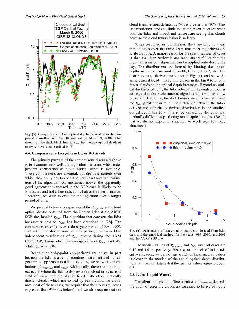
Simple Algorithm to Find Cloud Optical Depth The Open Atmospheric Science Journal, 2008, Volume 2 53
19.0 20.0 21.0 22.019.5 20.5 21.5 22.5
Time, UTC
0.01
0.1
1
10
Op
tical D
ep
th
empirical method, = (1.16/r 1)/((1 A)(1-g))
average of methods (Comstock et al., 2007)
direct beam, MFRSR, 415 nm
Cloud optical depthSGP Central Facility
March 9, 2000CIRRUS CLOUDS
Fig. (5). Comparison of cloud optical depths derived from the em-
pirical algorithm and the DB method on March 9, 2000. Also
shown by the thick black line is ave, the average optical depth of
many retrievals as described in [2].
4.4. Comparison to Long-Term Lidar Retrievals
The primary purpose of the comparisons discussed above
is to examine how well the algorithm performs when inde-
pendent verification of cloud optical depth is available.
These comparisons are essential, but the time periods over
which they apply are too short to permit a thorough evalua-
tion of the algorithm. As mentioned above, the apparently
good agreement witnessed in the SGP case is likely to be
fortuitous, and not a true indicator of algorithm performance.
Therefore, we wish to evaluate the algorithm over a longer
period of time.
We present below a comparison of the empirical with cloud
optical depths obtained from the Raman lidar at the ARCF
SGP site, labeled lidar. The algorithm that converts the lidar
backscatter data to lidar has been described in [28]. The
comparison extends over a three-year period (1998, 1999,
and 2000) but during most of this period, there was little
independent verification of lidar except during the ARM
Cloud IOP, during which the average value of lidar was 0.45,
while ave was 1.08.
Because point-by-point comparisons are noisy, in part
because the lidar is a zenith-pointing instrument and our al-
gorithm is applicable to a full sky view, we show the distri-
butions of empirical and lidar. Additionally, there are numerous
occasions where the lidar only sees a thin cloud in its narrow
field of view, but the sky is filled with other, optically
thicker clouds, which are sensed by our method. To elimi-
nate most of these cases, we require that the cloud sky cover
is greater than 95% (as before), and we also require that the
cloud transmission, defined as T/C, is greater than 80%. This
last restriction tends to limit the comparison to cases when
both the lidar and broadband sensors are seeing thin clouds
because the cloud transmission is so large.
When restricted in this manner, there are only 124 ten-
minute cases over the three years that meet the criteria de-
scribed above. A major reason for the small number of cases
is that the lidar retrievals are most successful during the
night, whereas our algorithm can be applied only during the
day. The distributions are formed by binning the optical
depths in bins of one unit of width, 0 to 1, 1 to 2, etc. The
distributions so derived are shown in Fig. (6), and show the
same general trend: many thin clouds in the bin 0 to 1, with
fewer clouds as the optical depth increases. Beyond an opti-
cal thickness of four, the lidar attenuation through a cloud is
so large that the backscattered signal is too small to allow
retrievals. Therefore, the distributions drop to virtually zero
for lidar greater than four. The difference between the lidar-
derived and empirically derived distribution in the smallest
optical depth bin (0 - 1) may be caused by the empirical
method’s difficulties predicting small optical depths. (Recall
that we do not expect this method to work well for these
situations).
0 1 2 3 4 5
cloud optical depth
0
0.2
0.4
0.6
0.8
1P
DF
empirical, median = 0.42
lidar, median = 1.0
Fig. (6). Distribution of thin cloud optical depth derived from lidar
data, and the empirical method, for the years 1999, 2000, and 2001 and the ACRF SGP site.
The median values of empirical and lidar over all cases are
0.42 and 1.0, respectively. Because of the lack of independ-
ent verification, we cannot say which of these median values
is closer to the median of the actual optical depth distribu-
tion; all we can state is that the median values agree to about
0.6.
4.5. Ice or Liquid Water?
The algorithm yields different values of empirical depend-
ing upon whether the clouds are assumed to be ice or liquid
54 The Open Atmospheric Science Journal, 2008, Volume 2 Barnard et al.
water. The type of cloud is represented in the calculation by
the choice of g, which we recommend be set to 0.87 and 0.8,
for liquid water and ice clouds respectively. An intermediate
value could be chosen for mixed phase clouds, but we have
not examined this case explicitly. The algorithm relies on
broadband measurements alone, and if these are the only
measurements available, one might wonder how to distin-
guish between ice and liquid water clouds. Based on the ex-
perience described above, where we obtained comparable
agreement between empirical and lidar using cloud transmis-
sion as a crude discriminator between ice and liquid clouds,
we suggest using a value of T/C as 0.8 to distinguish be-
tween the two types of clouds. In other words, we assume
that thin clouds are only ice clouds. However, if other in-
strumentation is deployed at a site, such as an infrared ther-
mometer (IRT) that senses cloud base temperature, then the
process of distinguishing between ice and water clouds could
be markedly improved.
5. CONCLUSIONS
We describe here the development and testing of an algo-
rithm for finding cloud optical depth from surface broadband
irradiance measurements. The derivation of this algorithm is
dependent on the assumptions of horizontal homogeneous
and optically thick clouds. Although the second of these as-
sumptions, by definition, will never be true for thin clouds,
and the first will rarely be true, we nevertheless apply the
method to the case of optically thin ice clouds, and find that
the method works surprising well. The algorithm is evalu-
ated by comparing our results with those from other retriev-
als and independent data. The evaluation is made much eas-
ier by the use of ice cloud data sets that have been studied
thoroughly as exemplified in the study of Comstock et al. [2]
and the TWP-ICE campaign The study of Comstock et al.
compares various algorithms and attempts algorithm verifi-
cation using independent data and flux closure studies. For
the TWP-ICE campaign, independent verification is avail-
able from aircraft sampling of ice cloud properties.
When applied to ice clouds, the algorithm may not work
well when the optical depth is low (0.1 or less), but seems to
work reasonably well, vis-à-vis other algorithms, for optical
depths from about 0.1 to 5.0, at least for the cases examined
here. We could not test the algorithm for larger values of ice-
cloud optical depth because we did not have data that in-
cludes ice clouds with optical depths that large. For the lim-
ited cases we examined here, the empirical cloud optical
depth and an independent determination of the optical depth
agreed to about 1 unit for the TWP-ICE case. For the SGP
case, the empirical optical depth roughly tracks an average
optical depth derived from other methods. In particular, for a
time series consisting of points when: (1) values of both ave
and empirical are available, and (2) empirical is greater than
zero, the median values obtained from these two methods are
0.79 ( ave) and 0.81 ( empirical) -- a difference of only 0.02
units. Such close agreement, however, is probably fortuitous
and unlikely to represent the performance of the algorithm,
thus suggesting the need for further evaluation. To achieve
this end we compare distributions of empirical to distributions
of optical depths derived from lidar data at the ACRF SGP
site over a three-year period. The median values of these
distributions over all cases are 0.42 and 1.0, for empirical and
lidar respectively, a difference of about 0.5. We remark,
however, that because of the lack of independent verification
over most of the three-year period, we cannot say which of
these median values most faithfully represents the actual
optical depth.
The algorithm would not be expected to work well for
isolated cirrus clouds because these cases contradict the as-
sumption of plane parallel conditions. Fortunately, these
cases can be eliminated using Long et al.’s [8] fractional sky
cover routine that can detect cases where the sky is mostly
clear. For smaller fractional sky covers, the DB method
could be used to infer , but this method would only provide
the optical depth of the clouds that are situated in the path
between the sun and earth.
Because of this method’s simplicity and its reliance on
standard shortwave irradiance measurements, it may be ap-
plied to estimate for both optically thin and optically thick
clouds at the many worldwide locations where such meas-
urements exist. However, when only broadband measure-
ments are available, it becomes problematic to distinguish
between thin ice clouds and thin liquid water clouds. This
problem can be mitigated by employing an infrared ther-
mometer (or similar instruments) to detect the cloud base
temperature. Absent such an instrument, we recommend
using the cloud transmission, T/C, as a crude discriminator
between ice and liquid clouds, with values of T/C > 0.8 sug-
gesting the presence of ice clouds.
ACKNOWLEDGEMENTS
This research was sponsored by the U. S. Department of
Energy’s Atmospheric Radiation Measurement Program
(ARM) under Contract DE-AC06-76RLO 1830 at Pacific
Northwest National Laboratory. Pacific Northwest National
Laboratory is operated by Battelle for the U.S. Department
of Energy. The authors wish to thank Dr. Chris Doran for his
comments regarding this work, and Nancy Burleigh and
Ruth Keefe for their help with this manuscript.
REFERENCES
[1] Turner DD, Vogelmann AM, Austin RT, et al. Thin liquid water
clouds - Their importance and our challenge. Bull Am Meteor Soc 2007; 88(2): 177-190.
[2] Comstock JM, d'Entremont R, DeSlover D, et al. An intercompari-son of microphysical retrieval algorithms for upper-tropospheric
ice clouds. Bull Am Meteor Soc 2007; 88(2): 191-204. [3] Barnard JC, Long CN. A simple empirical equation to calculate
cloud optical thickness using shortwave broadband measurements. J Appl Meteor 2004; 43(7): 1057-1066.
[4] Long CN, Ackerman TP. Identification of clear skies from broadband pyranometer measurements and calculation of downwel-
ling shortwave cloud effects. J Geophys Res 2000; 105(D12): 15609-15626.
[5] Dong XQ, Ackerman TP, Clothiaux EE, Pilewskie P, Han Y. Mi-crophysical and radiative properties of boundary layer stratiform
clouds deduced from ground-based measurements. J Geophys Res 1997; 102(D20): 23829-23843.
[6] Min QL, Harrison LC. Cloud properties derived from surface MFRSR measurements and comparison with GOES results at the
ARM SGP site. Geophys Res Lett 1996; 23(13): 1641-1644.

Simple Algorithm to Find Cloud Optical Depth The Open Atmospheric Science Journal, 2008, Volume 2 55
[7] Harrison L, Michalsky J, Berndt J. Automated multifilter rotating
shadow-band radiometer - an instrument for optical depth and ra-diation measurements. Appl Opt 1994; 33(22): 5118-5125.
[8] Long CN, Ackerman TP, Gaustad KL, Cole JNS. Estimation of fractional sky cover from broadband shortwave radiometer meas-
urements. J Geophys Res 2006; 111, doi: 10.1029/2005JD006475. [9] Shettle EP, Weinman JA. Transfer of solar irradiance through
inhomogeneous turbid atmospheres evaluated by eddingtons ap-proximation. J Atmos Sci 1970; 27(7): 1048-1055.
[10] Hu YX, Stamnes K. An Accurate parameterization of the radiative properties of water clouds suitable for use in climate models. J
Clim 1993; 6(4): 728-742. [11] Goody RM, Yung YL. Atmospheric Radiation, Theoretical Basis.
Oxford University Press, Oxford, New York, 1989. [12] Liou KN. Radiation and Cloud Processes in the Atmosphere. Ox-
ford University Press, Oxford, New York, 1992. [13] Heymsfield AJ, Bansemer A, Field PR, et al. Observations and
parameterizations of particle size distributions in deep tropical cir-rus and stratiform precipitating clouds: Results from in situ obser-
vations in TRMM field campaigns. J Atmos Sci 2002; 59(24): 3457-3491.
[14] McFarquhar GM, Um J, Freer M, Baumgardner D, Kok GL, Mace G. Importance of small ice crystals to cirrus properties: Observa-
tions from the Tropical Warm Pool International Cloud Experiment (TWP-ICE). Geophys Res Lett 2007; 34, doi: 10.1029/2007 GL0
29865. [15] Michalsky JJ, Anderson GP, Barnard J, et al. Shortwave radiative
closure studies for clear skies during the atmospheric radiation measurement 2003 aerosol intensive observation period. J Geophys
Res 2006; 111, doi: 10.1029/2005JD006341. [16] Younkin K, Long CN. Improved correction of IR loss in diffuse
shortwave measurements: An ARM Value Added Product. ARM TR-009, 2004; http: //www.arm.gov/publications/techreports.stm.
[17] Min QL, Joseph E, Duan MZ. Retrievals of thin cloud optical depth from a multifilter rotating shadowband radiometer. J Geophys Res
2004; 109, doi: 10.1023/2003JD003964.
[18] Yang P, Liou KN, Wyser K, Mitchell D. Parameterization of the
scattering and absorption properties of individual ice crystals. J Geophys Res 2000; 105(D4): 4699-4718.
[19] Stull R. An Introduction to Boundary Layer Meteorology. Kluwer Academic Press, Dordrecht, Boston, 1991.
[20] Long CN, Mather JH, Tapper N, Beringer J, Atkinson B. Surface radiation analysis from TWP-ICE. Proceedings of Sixteenth ARM
Science Team Meeting, Albuquerque, New Mexico, March 27-31, 2006, http: //www.arm.gov/publications/proceedings/conf16/exten-
ded_abs/long_cn1.pdf. [21] Gerber H, Takano Y, Garrett TJ, Hobbs PV. Nephelometer meas-
urements of the asymmetry parameter, volume extinction coeffi-cient, and backscatter ratio in Arctic clouds. J Atmos Sci 2000;
57(18): 3021-3034. [22] Ulanowski Z, Hesse E, Kaye PH, Baran AJ. Light scattering by
complex ice-analogue crystals. J Quant Spectrosc Radiat Transfer 2006; 100(1-3): 382-392.
[23] Schmitt CG, Iaquinta J, Heymsfield AJ. The asymmetry parameter of cirrus clouds composed of hollow bullet rosette-shaped ice crys-
tals from ray-tracing calculations. J Appl Meteor Climatol 2006; 45(7): 973-981.
[24] Um J, McFarquhar GM. Single-scattering properties of aggregates of bullet rosettes in cirrus. J Appl Meteor Climatol 2007; 46(6):
757-775. [25] Korolev A, Isaac GA. Relative humidity in liquid, mixed-phase,
and ice clouds. J Atmos Sci 2006; 63(11): 2865-2880. [26] Baumgardner D, Korolev A. Airspeed corrections for optical array
probe sample volumes. J Atmos Ocean Technol 1997; 14(5): 1224-1229.
[27] Strapp JW, Albers F, Reuter A, et al. Laboratory measurements of the response of a PMS OAP-2DC. J Atmos Ocean Technol 2001;
18(7): 1150-1170. [28] Comstock JM, Sassen K. Retrieval of cirrus cloud radiative and
backscattering properties using combined lidar and infrared radi-ometer (LIRAD) measurements. J Atmos Ocean Technol 2001;
18(10): 1658-1673.
Received: February 11, 2008 Revised: March 11, 2008 Accepted: March 18, 2008


![archive.iypt.orgarchive.iypt.org/...spaghetti_Iran_HG_HA_v1.docx · Web viewIn this article we present a new simple algorithm using numerical methods to find ... [7] K.Sankara Rao](https://static.fdocuments.us/doc/165x107/5a71a9f27f8b9aa2538d0ac5/archiveiyptorgarchiveiyptorgspaghettiiranhghav1docxdoc.jpg)