Ann Oper Res (2011) 186:275–293DOI 10.1007/s10479-011-0898-z

A simple and effective algorithm for the MaxMindiversity problem

Daniel Cosmin Porumbel · Jin-Kao Hao · Fred Glover

Published online: 15 May 2011© Springer Science+Business Media, LLC 2011

Abstract The challenge of maximizing the diversity of a collection of points arises in avariety of settings, including the setting of search methods for hard optimization problems.One version of this problem, called the Maximum Diversity Problem (MDP), produces aquadratic binary optimization problem subject to a cardinality constraint, and has been thesubject of numerous studies. This study is focused on the Maximum Minimum DiversityProblem (MMDP) but we also introduce a new formulation using MDP as a secondaryobjective. We propose a fast local search based on separate add and drop operations and onsimple tabu mechanisms. Compared to previous local search approaches, the complexity ofsearching for the best move at each iteration is reduced from quadratic to linear; only certainstreamlining calculations might (rarely) require quadratic time per iteration. Furthermore,the strong tabu rules of the drop strategy ensure a powerful diversification capacity. Despiteits simplicity, the approach proves superior to most of the more advanced methods from theliterature, yielding optimally-proved solutions for many problems in a matter of seconds andeven attaining a new lower bound.

Keywords Maximum diversity · MaxMin diversity · Tabu search

1 Introduction

Let Z be a finite collection of points (elements), and let Z(k) = {X ⊂ Z : |X| = k}, the setof all k element subsets of Z, where 2 ≤ k ≤ |Z| − 1. Associated with each pair of points

D.C. PorumbelUArtois, LGI2A, Univ. Lille-Nord de France, Technoparc Futura, 62400 Béthune, Francee-mail: daniel.porumbel@univ-artois.fr

J.-K. Hao (�)LERIA, Université d’Angers, 2 Boulevard Lavoisier, 49045 Angers Cedex 01, Francee-mail: hao@info.univ-angers.fr

F. GloverOptTek Systems, Inc., 4421 17th Street, Boulder, CO 80302, USAe-mail: glover@opttek.com

276 Ann Oper Res (2011) 186:275–293

x, y ∈ Z is a real number d(x, y) (= d(y, x)) called a distance. (In our formulation, d(x, y)

does not have to satisfy the properties of a customary distance metric and may even benegative.) For simplicity, when referring to d(x, y) we understand that x �= y. The classicalMaximum Diversity Problem (MDP) requires identifying a set X∗ ∈ Z(k) that maximizesthe sum of the distances d(x, y) over all distinct pairs x, y ∈ X∗. More precisely, the problemmay be expressed as:

MDP : FindX∗ = arg max

( ∑x,y∈X

d(x, y) : X ∈ Z(k)

).

A number of computational studies of MDP have been performed, including those of Kuoet al. (1993), Ghosh (1996), Glover et al. (1998), Silva et al. (2004), Andrade et al. (2005),Duarte and Marti (2007), Gallego et al. (2009), Palubeckis (2007), Aringhieri et al. (2008),Santos et al. (2008), Wang et al. (2009) and Aringhieri and Cordone (2011). As observedin Kuo et al. (1993) the maximum diversity problem has applications in plant breeding, so-cial problems, ecological preservation, pollution control, product design, capital investment,workforce management, curriculum design and genetic engineering.

In certain contexts, however, a more useful definition of diversity involves the goal offinding a set X∗ in Z(k) that maximizes the minimum distance between the points x, y ∈ X∗instead of the sum of the distances between these points. This “MaxMin” form of diversityhas application to achieving diversification goals for metaheuristics, as noted in Glover andLaguna (1997), and is relevant to the area of simulation optimization (see, e.g., April et al.2003). To capture this form of diversity, the classical definition of the MaxMin DiversityProblem (MMDP) may be expressed as:

MMDP : FindX∗ = arg max(

Minx,y∈X

(d(x, y) : X ∈ Z(k))).

Methods for the MMDP problem, both heuristic and exact, have been proposed and inves-tigated by several authors, including Erkut (1990), Kincaid (1992) and Ghosh (1996) andDella Croce et al. (2009). A comprehensive survey of previous work can be found in Re-sende et al. (2010).

In terms of practical results for MMDP, there are two very recent studies that achievedvery high performances, thus providing a solid comparison base for benchmarking new al-gorithms. Resende et al. (2010) presented a refined GRASP (with Path Relinking) approach,as well as extensive comparisons with previous algorithms (e.g. Erkut 1990; Kincaid 1992;Ghosh 1996). Della Croce et al. (2009) described an algorithm which uses a powerful cliqueheuristic (i.e., Grosso et al. 2008) as an internal component in a dichotomic search. Thisalgorithm reached very competitive bounds—including several that the authors proved op-timal using an exact clique solver Östergård (2002).

The objective of this paper is to present a simple and effective approach to diversity prob-lems, using a new MMDP formulation based on both MMDP and MDP (Sect. 2.1). To dealwith this problem, we first apply a constructive heuristic (Sect. 2.2), and then we place aspecial emphasis on a new tabu search algorithm based on separate drop and add opera-tions (Sect. 2.3). The proposed search approach aims at meeting two essential challenges inheuristic algorithm design. First, in order to render the search process as fast as possible,the computational complexity of the neighborhood exploration is reduced to linear and allcalculations are effectively streamlined. Secondly, the search process can not get stuck bykeeping certain elements of a solution assignment in the selected set X for an indefinite du-ration, because each selected element is systematically dropped after a determined numberof iterations.

Ann Oper Res (2011) 186:275–293 277

The paper is organized as follows. Section 2 is devoted to a detailed presentation of theconstructive stage and of the new search algorithm based on drop and add moves. Numericalresults are presented in Sect. 3, followed by conclusions in Sect. 4. The Appendix providesdetailed instance-by-instance comparisons between our approach and state-of-the-art algo-rithms.

2 The proposed approach

The main component of our approach is a simple tabu search algorithm that is very fast(the iteration complexity is reduced to minimum) and that exhibits strong diversificationqualities. While several search methods for MMDP or MDP are already available in theliterature (see Introduction), they typically use a neighborhood of quadratic cost based onswap moves, i.e., a neighbor is obtained by replacing a selected element with a non-selectedone. A novelty of our search strategy is that such swap moves are executed as a successionof two separate steps: drop and add. These two steps have linear complexity; furthermore,all calculations are effectively streamlined, and so, the total iteration computational costbecomes considerably less expensive than in other approaches. The drop operation alwaysremoves the “oldest” selected element: each selected point is replaced with a different oneafter exactly k iterations. This simple policy, which represents an elementary instance ofa short-term tabu search rule, proves very effective in helping the search process to avoidlooping and ensure diversity.

2.1 Problem formulation

We are interested in going beyond the classical formulation of MMDP to give a more generalformulation that includes the objective of MDP as a secondary objective, i.e., we seek firstto maximize the minimum distance between points in the chosen set X∗ and subject to thisalso seek to maximize the sum of the distances between these points. The inclusion of thissecondary objective is motivated by the fact that there may be a number of solutions thatqualify as optimal when the MMDP objective is considered solely by itself, and thereforeit is useful to have a meaningful way to differentiate among these “tied optimal” solutions,particularly by means of a criterion such as that of MDP which has also been found ofinterest in the literature. This formulation is also motivated by observations of Glover et al.(1998) that it can be important to differentiate among solutions that are equally valued byreference to the classical objective.

Formally, define Zo(k) = {Xo = arg max(Minx,y ∈ X(d(x, y) : X ∈ Z(k))}. Then wemay write the more general form of MMDP, denoted MMDPo as

MMDPo: FindX∗ = arg max

( ∑x,y∈Xo

d(x, y) : Xo ∈ Zo(k)

). (1)

Alternatively, we may also state MMDPo by referring to a small positive number ε (chosenso that the maximization of the summed distances is subordinate to the maximization of themin distance) and writing

X∗ = arg max

(Minx,y∈X

(d(x, y) + ε

∑x,y∈X

d(x, y) : X ∈ Z(k)

)). (2)

278 Ann Oper Res (2011) 186:275–293

We will call the objective function of MMDPo, variously expressed in the form of (1) or (2)as the MMDPo criterion. Clearly a solution that is optimal for MMDPo will also be optimalfor MMDP, though the converse is not true.

2.2 Constructive procedure for MMDPo

The first stage (see Algorithm 1 below) of our framework consists of an elementary con-structive algorithm to create a set X in Z(k) that constitutes a first candidate for an optimalsolution.

Algorithm 1 (Constructive Algorithm)Choose an initial point x∗ ∈ Z and set X(1) = {x∗}.Set h = 1.While h < k:

Set h := h + 1 and choose a point x∗ ∈ Z − X(h − 1) such thatx∗ = arg max(Min(d(x, y) : x ∈ Z − X(h − 1), y ∈ X(h − 1))),

where ties for x∗ are broken by selecting a point that maximizes∑

d(x, y).Set X(h) = X(h − 1) ∪ {x∗}.

EndwhileIdentify the first candidate for an optimal MMDPo solution by X∗ = X(k).

The initial point x∗ to include in X(1) = {x∗} is obtained by selecting a point x∗ thatmaximizes the sum of distances towards the other points. The algorithm, which dependsimportantly on this initial x∗, is a greedy algorithm for passing from X(h − 1) to X(h) byreference to the MMDP objective, subject to breaking ties relative to the MDP objective.

The set X∗ = X(k) produced at the final stage of this constructive stage is then modifiedby the Drop-Add search described next.

2.3 Simple tabu search algorithm based on drop and add moves

Both the constructive and the search algorithms make use of an iteration counter, denotedby iter, that progresses from 1 through k as the successive steps of the Constructive Algo-rithm are executed, and continues to be incremented by 1 at each subsequent iteration ofthe Drop-Add Simple Tabu Search Algorithm that follows. For each point x that belongs toa current set X(k), we let iter(x) denote the iteration at which x was added to X(k). Thelocal search also drops elements from X(k), and for each x that is dropped, we likewise letiter(x) identify the iteration at which x was removed from X(k). (Initially, iter(x) = 0 forall x ∈ Z.) Hence, more precisely, iter(x) denotes the latest iteration at which x was eitheradded to or dropped from X(k).

We refer to a subset AddX(k) of the current set of points Z − X(k) that consists ofeligible add points, that is, those eligible to be considered for being added to X(k). We defineAddX(k) as Z −X(k), and so, all points outside of X(k) are eligible to be added. Similarly,we also refer to a subset of eligible drop points DropX(k): this set employs an exceedinglysimple tabu rule by always containing only the “oldest” point in X(k), i.e., the point x# =arg min(iter(x) : x ∈ X(k)). By this definition, the value of iter(x#) can be identified asiter(x#) = iter− (k −1), where iter denotes the current value of the iteration counter. Hence,at the end of the Constructive Algorithm, iter = k and iter(x#) = 1, identifying x# as the firstpoint added to X(k).

Ann Oper Res (2011) 186:275–293 279

Algorithm 2 below presents the algorithmic template of the proposed local search. Thefirst step simply drops the “oldest selected point”, i.e., the selected point x# ∈ X(k) thatverifies iter(x#) = iter − (k − 1). This operation temporarily produces a set X(k − 1); af-terwards, Step 2 chooses the point x∗ from AddX(k) by the same criterion used in theConstructive Algorithm, i.e., x∗ is chosen to maximize the minimum distance from x∗ toany point in X(k − 1), and, subject to this, to maximize the sum of the distances to thepoints in X(k − 1). Step 3 updates the value of X∗ if X(k) is better than the best visited so-lution so far. Finally, iter(x#) and iter(x∗) are updated; the iteration counter is incrementedin the last instruction.

Algorithm 2 (Drop-Add Simple Tabu Search)While a termination condition is not satisfied:

1. From the current set X(k), select the point x# ∈ DropX(k) to produce the setX(k − 1) = X(k) − {x#}.

2. Choose a point x∗ ∈ AddX(k) = Z − X(k) such thatx∗ = arg max(Min(d(x, y) : x ∈ AddX(k), y ∈ X(k − 1))),

breaking ties for x∗ by selecting a point that maximizes (∑

d(x, y) : y ∈ X(k − 1))

Set X(k) = X(k − 1) ∪ {x∗}.3. If X(k) improves on the best set X∗ by the MMDPo criterion Then

Record X(k) as the new X∗End If

4. Set iter(x#) = iter(x∗) = iter; Set iter := iter + 1.

End While

The method stops when no improvement according to the MMDPo criterion is made inX∗ for a number of iterations, denoted as maxNoGain in Sect. 3.

2.4 Streamlining the calculations

An important objective of the proposed search strategy is to avoid performing iterationsof quadratic complexity. Since Step 2 of Algorithm 2 requires going through all points ofAddX(k) = Z − X, it is important to be able to access certain information in O(1)—e.g.,the minimum distance from each point x ∈ Z −X to points from X (denoted by MinDist(x)

below). For this purpose, we maintain and update the following three records for each x ∈ Z

after each add or drop operation:

• MinDist(x) = Min{d(x, y) : y ∈ X},• SumDist(x) = (

∑d(x, y): y ∈ X),

• MinDistCount(x) = |{y ∈ X : d(x, y) = minDist(x)}|, i.e., the number of elements hav-ing x as the closest point.

Each of these records refers to distances from a given point x to points within X, whether ornot x lies in X. As indicated, we use minDist(x) + εSumDist(x) as the criterion to evaluatea point x ∈ Z − X to be added to X, by selecting a point that minimizes this criterion. Thus,the ability to quickly update the value of MinDist(x) and SumDist(x) without always havingto do the full calculations indicated in their preceding definitions saves significant effort. Weshow next how to establish a complexity bound for the streamlining calculations of O(|Z|)in the average case (the worst case complexity is O(|Z| · |X|), but it is not reached for mostiterations).

280 Ann Oper Res (2011) 186:275–293

After adding a point x∗, it is necessary to examine all x ∈ Z − {x∗} and: (i) updateMinDist(x) and initialize MinDistCount(x) to 1 if d(x, x∗) < MinDist(x), or (ii) updateonly MinDistCount(x) if d(x, x∗) = MinDist(x), or (iii) do not modify MinDist(x) orMinDistCount(x) if d(x, x∗) > MinDist(x). In addition, SumDist(x) is always increasedby d(x, x∗); the records of x∗ do not require any change. All these calculations can alwaysbe performed in O(|Z|) using Algorithm 3 below.

Algorithm 3 (Calculation streamlining after adding an element x∗)For Each x ∈ Z − {x∗}

SumDist(x) = SumDist(x) + d(x, x∗)If (d(x, x∗) = MinDist(x)) Then

MinDistCount(x) = MinDistCount(x) + 1Else If (d(x, x∗) < MinDist(x))

MinDistCount(x) = 1MinDist(x) = d(x, x∗)

End IfEnd For Each

The update after dropping point x# requires going through all x ∈ Z − {x#} and, foreach x, one of the following situations may arise:

(1) do not modify MinDist(x) or MinDistCount(x), if d(x, x#) > MinDist(x);(2) decrement MinDistCount(x), if MinDistCount(x) > 1 and d(x, x#) = MinDist(x);(3) recalculate MinDist(x), if MinDistCount(x) = 1 and d(x, x#) = MinDist(x).

Notice that the records of x# do not require any modification. Algorithm 4 below presentsall update calculations that are executed after dropping x#.

Algorithm 4 (Update calculations after dropping an element x#)For Each x ∈ Z − {x#}

SumDist(x) = SumDist(x) − d(x, x#)

If (d(x, x#) = MinDist(x)) ThenIf (MinDistCount(x) > 1) Then

MinDistCount(x) = MinDistCount(x) − 1 (case (2))Else

Re-calculate MinDist(x) and MinDistCount(x) (case (3))Endif

End IfEnd For Each

From all three situations above, case (3) is the most problematic one because it requiresrecalculating MinDist(x). Such an update can be performed in linear time for any particu-lar x. In the worst case, all elements x ∈ Z−{x#} would require such a recalculation, leadingto a quadratic time complexity for the whole Algorithm 4. However, even this theoreticallyquadratic cost can only reach O(|Z| · |X|) at maximum, less computationally expensivethan O(|Z|2).

Furthermore, in practical terms, the impact of this quadratic worst-case complexity islimited. Indeed, the above O(|Z| · |X|) recalculations are not required at each iteration, be-cause case (3) can not arise systematically. Furthermore, even for the iterations that do re-quire these recalculations, the O(|Z| · |X|) complexity can be reached only if O(|Z|) points

Ann Oper Res (2011) 186:275–293 281

from Z would require updating MinDist(x) and MinDistCount(x). Such a situation couldonly arise if x# would be the unique closest point to most of the other points from Z. Thiscondition is quite strong, and consequently, such a high complexity is not often reached inpractice. In most of the cases, there is only a bounded number of points x ∈ Z having x#

as the unique closest point, and so, we observe that the average complexity of the updateoperation (over all iterations) is O(|Z|).

Finally, since k = |X| is often significantly smaller than n = |Z| (e.g., in our standardinstances, k is either 0.1 · n or 0.3 · n), the implementation should avoid going through allelements of Z when one only needs to iterate through the elements of X. As such, a state-ment of the form “For each x ∈ Z, if selected[x] then” should be avoided because it hascomplexity O(|Z|) > O(|X|). For this purpose, it is important to record X both as a simple0–1 array and as a linked list that can be processed in O(|X|) time with the appropriate datastructures.

2.5 Complexity remarks compared with classical approaches

To compute the total iteration complexity, we first observe that Step 1 of Algorithm 2 re-quires O(1) time. Selecting the best x∗ in Step 2 requires going through all elements ofAddX(k) in O(|Z − X|) < O(|Z|) time (for each x, the values Min(d(x, y) : y ∈ X(k − 1))

and∑

d(x, y) : y ∈ X(k − 1) are stored in two vectors that are updated by the streamliningroutines). Furthermore, the above section showed that the streamlining calculations requireO(|Z|) time for most iterations, or O(|Z| · |X|) time in the worst case. As such, the totalworst case iteration complexity is O(|Z| · |X|), less than O(|Z|2) in other local search meth-ods. However, compared to previous approaches, the complexity improvement is even morepronounced in the average case, i.e., O(|Z|) compared to O(|Z|2).

Indeed, most previous local search methods from the literature (see e.g., Erkut 1990or Ghosh 1996) consider a quadratic neighborhood, commonly defined as the set of allpotential solutions that can be reached by applying a swap on the current solution, i.e., aneighborhood transition consists of swapping an element a ∈ X(k) with an element b ∈Z − X(k). The evaluation of such a neighborhood requires quadratic time in the worst caseas well as in the average case. In contrast, most iterations of our algorithm do not requiremore than O(|Z|)—i.e., only the streamlining routines could require O(|Z| · |X|) and onlywhen the current potential solution verifies certain strong conditions (see Sect. 2.4).

Besides a faster evaluation of a smaller neighborhood, our approach provides easier pro-cedures for ensuring diversification, taking advantage from the tabu mechanism underlyingdrop moves. (There is obviously no virtue in using a simpler neighborhood if this is not ac-companied by procedures that ultimately compensate for potential loss of information thatwould otherwise be processed at each iteration.) The elementary type of tabu search rule,which defines DropX(k) to contain only the “oldest” selected point in X(k), causes each se-lected point to stay selected for exactly k iterations. A useful feature of this approach is that,after removing point x#, the algorithm can not immediately add x# back because it needs toadd a point x∗ from AddX(k) = Z−X(k). If x# would be added back in the future, it wouldbe added into a configuration that will have changed in the meantime, and looping wouldbe thus avoided. We also tried using larger sets DropX(k), but our experiments showed nosignificant or conclusive improvement. Indeed, this simple approach appears rather robustrelative to the chosen size of AddX and DropX.

Furthermore, we also tested more complex techniques such as interleaving Constructiveand local search methods, as well as more advanced local search algorithms, e.g., usinglarger neighborhoods and more complex evaluations of points to add or to drop. While it is

282 Ann Oper Res (2011) 186:275–293

always possible to refine and achieve a certain improvement using such techniques, the goalof this paper is only to present a simple, effective and very practical algorithm: aside fromthe termination condition (i.e., maxNoGain), one does not even need any parameter tuning.

3 Computational experiments

This section is devoted to computational assessments,1 as well as to comparisons with themost recent and best performing MMDP approaches: DCGL from Della Croce et al. (2009)and RMGD from Resende et al. (2010). The DCGL approach starts out by sorting the dis-tance values. Each distance value � has an associated clique problem that can only be solvedif the MMDP optimum is lower than �. Based on a powerful clique algorithm, DCGL ap-plies a dichotomic search to rapidly find distance values for which the clique problem canbe solved. RMGD proposes a completely different approach based on exploiting existingconstructive and local search methods, combined with powerful new techniques based onGRASP (with new local improvement operators), Path-relinking and Evolutionary Path Re-linking.

Following the experimental protocol from the DCGL and RMGD papers, we consider120 MMDP instances,2 belonging to two classes: Geo and Ran. Each of these two classescontains 60 instances that can be further classified into three groups, according to the car-dinal of Z : n = |Z| = 100, n = 250 or n = 500. Each group contains 20 instances, half ofthem with k = 0.1 · n, and half with k = 0.3 · n.

We will first present the results as summary tables (see Tables 1–5), using the formatfrom the RMGD paper. To be specific, we provide the following three indicators for eachgroup of 20 instances:

Deviation (%) the average deviation from the best MMDP lower bound from the literature(representing the best solution ever obtained by other researchers). For instance, given aninstance with a best known lower bound value of 100, a solution of 80 has a deviation of20%; the average deviation over all instances is reported.

#Best the number of instances for which the best known lower bound is reached.TimeAvg the average time spent by the algorithm in seconds. The reported CPU times are

obtained on a 2.8 GHz Xeon processor using the C++ programming language compiledwith the –O2 optimization option (gcc version 4.1.2 under Linux).

Besides these summaries, we also provide (in Appendix) detailed results, as well asinstance-by-instance comparisons with DCGL and RMGD. For supplementary information,we also provide the objective value according to MDP criterion.

The stopping condition is to terminate upon reaching a maximum number of iterations(maxNoGain) with no improvement of the best value of the MMDPo objective function. Wepresent results with three stopping conditions: maxNoGain = 5 ·n, maxNoGain = 10000 ·n,and maxNoGain = 2000000 ·n. Comparing to other papers from the MMDP literature, theseconditions respectively correspond to: very short execution times (<1 second), moderateexecution times (several tens of seconds at maximum) and high execution times (one toseveral hours). It is worth reiterating that maxNoGain is the only parameter required by ouralgorithm.

1The source code of our algorithm and the solutions for the largest instances with n = 500 are available at:http://www.info.univ-angers.fr/pub/hao/mmdp/.2Available at http://www.uv.es/rmarti/paper/mdp.html.

Ann Oper Res (2011) 186:275–293 283

Table 1 Summary results of theconstructive algorithm Instance group Deviation #Best Avg. Time (sec)

Geo 100 6.41% 0 <0.1

Geo 250 4.10% 0 <0.1

Geo 500 6.11% 0 <0.1

Ran 100 6.17% 0 <0.1

Ran 250 4.56% 0 <0.1

Ran 500 21.40% 0 <0.1

All 120 instances 8.13% 0 <0.1

Table 2 Drop-Add Searchsummary results formaxNoGain = 5 · n

Instance group Deviation #Best Avg. Time (sec)

Geo 100 1.64% 2 <0.1

Geo 250 1.70% 0 <0.1

Geo 500 2.59% 0 <0.1

Ran 100 3.55% 4 <0.1

Ran 250 2.84% 0 <0.1

Ran 500 11.50% 0 <0.1

All 120 instances 3.97% 6 <0.1

3.1 Results of the constructive algorithm

We first present (Table 1) the summarized results of the constructive algorithm described inSect. 2.2. This constructive stage stops as soon as k elements are selected.

While this constructive heuristic does not yield solutions of impressive quality comparedto those obtained by methods that run for longer durations, the quality is nevertheless note-worthy in view of the amount of time invested in reaching these solutions.

3.2 Results of the Drop-Add search algorithm

The Drop-Add search algorithm is launched from an initial solution provided by the con-structive stage. The summarized results, group by group, are presented in Tables 2–4; eachtable corresponds respectively to one of the three stopping conditions mentioned above.

The first table from these summaries (Table 2) shows that our algorithm can reach quitecompetitive performances in less than 0.1 seconds. More precisely, given the very low run-ning times associated to the first stopping condition (i.e., maxNoGain = 5 · n), a deviationfrom the optimum of less than 4% is somewhat surprising, representing a value that mightbe considered acceptable in many applications.

Table 3 presents the results associated with an intermediate stopping condition(maxNoGain = 10000 · n); our algorithm manages to reach a large proportion (97 over 120)of the best known lower bounds within a moderately short time. For illustration, the Drop-Add search algorithm can solve in 2–3 seconds all benchmark instances with n = 100—i.e., Geo 100 and Ran 100 (the optimality of these bounds is proved in the DCGL pa-per). In slightly more than 10 seconds, the algorithm also reaches all proved optima of all

284 Ann Oper Res (2011) 186:275–293

Table 3 Drop-Add Searchsummary results formaxNoGain = 10000 · n

Instance group Deviation #Best Avg. Time (sec)

Geo 100 0.00% 20 2

Geo 250 0.10% 15 13.5

Geo 500 0.31% 8 77.9

Ran 100 0.00% 20 2

Ran 250 0.00% 20 12.3

Ran 500 0.53% 14 58.7

All 120 instances 0.15% 97 27.7

Table 4 Drop-Add Searchsummary results formaxNoGain = 2000000 · n

Instance group Deviation #Best Avg. Time (sec)

Geo 100 0.00% 20 449.7

Geo 250 0.06% 17 2737

Geo 500 0.11% 16 14093

Ran 100 0.00% 20 454.4

Ran 250 0.00% 20 2499

Ran 500 0.08% 19 12034

All 120 instances 0.04% 112 5378

Ran instances with n = 250 with k = 25. By allowing longer running times (i.e., usingmaxNoGain = 2000000 · n), our algorithm reaches 112 best lower bounds out of 120, seeTable 4. The average deviation from the best value of MMDP objective function becomes0.04%, almost negligible.

3.3 Comparison with related heuristics

In order to better evaluate the impact of the proposed ideas, we compare our approach withtwo related local search methods and a population-based heuristic:

− Swap-LS: A basic local search using a swap-based neighborhood of quadratic size. Es-sentially, an iteration of this algorithm consists of searching the best swap between aselected and a non-selected element, hence the quadratic complexity of an iteration.

− GhoC+BLS: An algorithm using the GhoC constructive method due to Ghosh (1996),followed by the local search BLS studied in Erkut (1990) and Ghosh (1996). This localsearch algorithm also utilizes a swap-based quadratic neighborhood.

− Grasp+EvPR: Evolutionary Path-relinking combined with a GRASP algorithm based ona classical constructive method and a significantly improved local search (Resende et al.2010).

The implementation of Swap-LS is derived by extending the code of our Drop-Addsearch algorithm. Regarding GhoC+BLS and Grasp+EvPR, we make use of the resultsprovided by the RMGD paper—the detailed results from the RGMD paper are publiclyavailable on-line at heur.uv.es/optsicom/mmdp/. However, we needed to recalculate the sum-maries using the updated bounds provided by the DCGL paper.

Ann Oper Res (2011) 186:275–293 285

Table 5 Comparison between Drop-Add Search (using maxNoGain = 10000 · n, as in Table 3) and threeother heuristics using local search

Instance group Drop-Add Search Swap-LS GhoC+BLS Grasp+EvPR

Dev #Best Time Dev #Best Time Dev #Best Time Dev #Best Time

[%] [s] [%] [s] [%] [s] [%] [s]

Geo 100 0 20 2 0.95 4 2 0.75 10 2 0.09 17 4

Geo 250 0.1 15 13.5 1.29 0 16.05 1.30 0 30 0.47 4 66

Geo 500 0.31 8 77.9 1.4 0 91.6 3.17 0 282 0.88 0 1465

Ran 100 0 20 2 4.42 1 2 1.71 4 1 0.49 15 7

Ran 250 0 20 12.3 3.66 0 12.7 3.26 0 16 1.53 6 271

Ran 500 0.53 14 58.7 21.3 0 66.65 13.52 0 93 11.34 0 6349

All 120 instances 0.15 97 27.7 5.51 5 31.83 3.95 14 71 2.47 42 1360

Table 5 presents the actual comparison between our Drop-Add search algorithm and thesethree algorithms. The same indicators as in Sect. 3.2 are used: the average deviation fromthe optimum (Dev [%]), the number of best-known bounds reached (#Best) and the time inseconds (Time [s]). The Drop-Add search algorithm used a very moderate computing timecompared to the other three algorithms.

Although the results from Table 5 are not all obtained in the same technical en-vironment (i.e., the first two and the last two algorithms were implemented by dif-ferent authors on different platforms), they do offer some indications as to the rela-tive performance of the algorithms. Comparing to a quadratic swap-based local search(see Swap-LS, as well as GhoC+BLS), our Drop-Add Search algorithm obtains clearlyimproved results using a similar or smaller amount of time. Even compared to morecomplex heuristics based on Evolutionary Path-relinking (hybridized with an enhancedlocal search), our approach is highly competitive and is able to rapidly reach estab-lished bounds in numerous cases (see also the instance-by-instance comparisons inSect. 3.4).

Notice that in this comparison, the Drop-Add Search is not given an advantage com-pared to Swap-LS, either in terms of computing time, or in terms of equivalent evaluationcounts. Indeed, Table 5 shows that Swap-LS always uses more time than Drop-Add Search(compare columns 7 and 4). This is due to the fact that the stopping condition is more per-missive in Swap-LS: while the Drop-Add Search uses maxNoGain = 10000 · n, Swap-LSstops after maxNoGain = 15000 · n swap evaluations. Since an iteration of Swap-LS con-sists of searching for the best swap between a selected and an unselected element, such aniteration evaluates a quadratic number of swaps. Consequently, the computational effort ofone iteration of our Add-Drop algorithm is roughly equivalent to a single swap evaluation,rather than to a complete (quadratic complexity) Swap-LS iteration. Furthermore, we con-firm that the number of swap evaluations always exceeds or is comparable to the number ofDrop-Add iterations. Given the difficulty of comparing different methods, the comparisonsshown above are provided for indicative purposes and should be interpreted with a word ofcaution.

3.4 Detailed comparisons and instance-by-instance results

Additional instance-by-instance outcomes are reported in Tables 6 and 7 (Appendix), fol-lowing the format from the DCGL paper. In both tables we used the intermediate stopping

286 Ann Oper Res (2011) 186:275–293

condition maxNoGain = 10000 · n, as in Tables 3 and 5. The total computing time (tens ofseconds, at maximum) can be considered reasonably moderate compared to other methodsfrom the literature. Indeed, our algorithm required an average time of 31.17 seconds for theGeo instances and an average time of 24.35 seconds for the Ran instances. The best methodsamong those tested by the RMGD paper required hundreds of seconds; the DCGL algorithmrequired average times of tens of seconds as well.

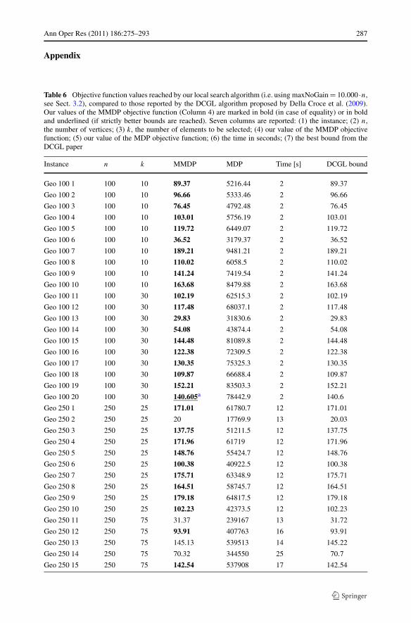
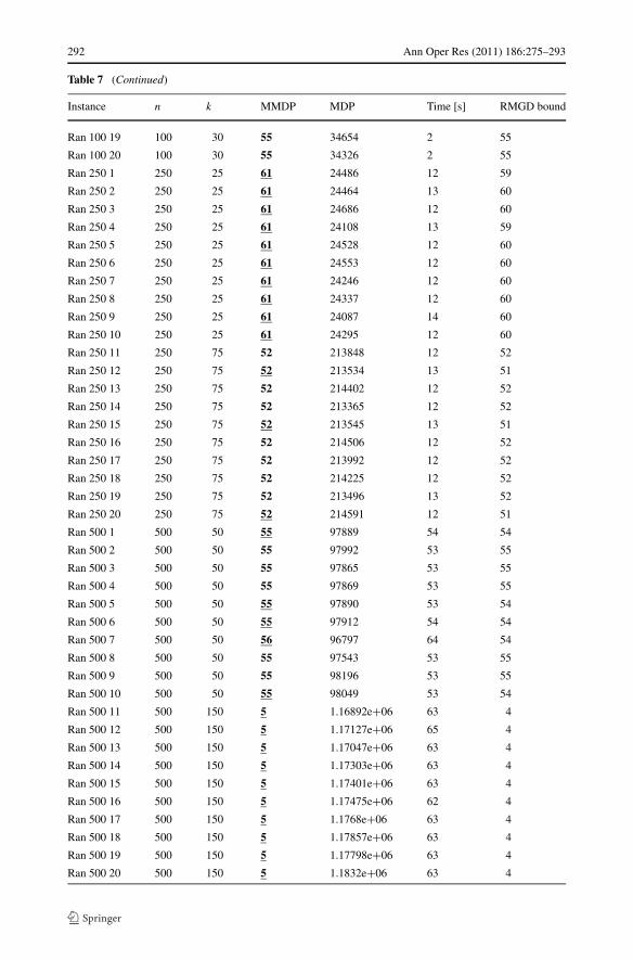
Table 6 shows that the Drop-Add search algorithm achieves a level of performance ona par with that of the DCGL approach—although DCGL utilizes as an internal compo-nent a more complex and refined max-clique algorithm presented in Grosso, Locatelli andPullan (2008). Furthermore, Table 7 presents an instance-by-instance comparison with thebest bounds reported by the RMGD paper (also, individual results of two algorithms fromRMGD are summarized Table 5). Besides the fact that our algorithm is very fast,3 it alwaysreaches the best RMGD bounds and even improves upon these best bounds in more than 60instances.

4 Conclusions

We have presented a simple approach for MMDP that nevertheless proves surprisingly ef-fective. For example, the proposed Drop-Add Simple Tabu Search finds within several sec-onds all optimally-proved solutions for all standard benchmark instances with n = 100, aswell as for certain instances with n = 250. The algorithm is competitive with more refinedapproaches from the literature, and even outperforms several methods tested in Resendeet al. (2010), e.g., methods that refer to Simulated Annealing, Tabu Search (based on adifferent foundation, using classical swap-based quadratic neighborhoods), GRASP withpath-relinking, GRASP with evolutionary path-relinking, etc. By allowing reasonably largeramounts of time, our approach reached almost all best-known lower bounds—reported bythe algorithm of Della Croce et al. (2009). We also report a solution better than the previousbest known solution to the benchmark instance “Ran 500 3”, establishing a new MMDPlower bound of 56 (the previous best-known bound was 55).

As detailed in Sect. 2.5, the effectiveness of the new approach, which utilizes an ex-tremely simple type of tabu search rule, derives from a low iteration complexity and fromstrong diversification qualities of the search process. Indeed, apart from the streamlining cal-culations that rarely require more than linear time, the complexity of an iteration is O(|Z|)—computationally less expensive than O(|Z|2) in other local search-based algorithms. Besidessuch speed benefits, important diversification properties arise from the fact that the simpletabu rule causes each selected element to be systematically dropped after a fixed period oftime.

Acknowledgements We are grateful to the reviewers of the paper for their helpful comments and sugges-tions. This work was partially supported by the Region of “Pays de la Loire” (France) within the Radapop(2009-2012) and LigeRO (2010-2013) Projects.

3We do not claim that such speed comparisons are absolute. Recall our reported CPU times are obtained ona 2.8 GHz Xeon processor using the C++ programming language compiled with the -O2 optimization flag(gcc version 4.1.2 under Linux). RMGD and DCGL used Pentium IV processors running at 3–3.2 GHz.

Ann Oper Res (2011) 186:275–293 287

Appendix

Table 6 Objective function values reached by our local search algorithm (i.e. using maxNoGain = 10.000 ·n,see Sect. 3.2), compared to those reported by the DCGL algorithm proposed by Della Croce et al. (2009).Our values of the MMDP objective function (Column 4) are marked in bold (in case of equality) or in boldand underlined (if strictly better bounds are reached). Seven columns are reported: (1) the instance; (2) n,the number of vertices; (3) k, the number of elements to be selected; (4) our value of the MMDP objectivefunction; (5) our value of the MDP objective function; (6) the time in seconds; (7) the best bound from theDCGL paper

Instance n k MMDP MDP Time [s] DCGL bound

Geo 100 1 100 10 89.37 5216.44 2 89.37

Geo 100 2 100 10 96.66 5333.46 2 96.66

Geo 100 3 100 10 76.45 4792.48 2 76.45

Geo 100 4 100 10 103.01 5756.19 2 103.01

Geo 100 5 100 10 119.72 6449.07 2 119.72

Geo 100 6 100 10 36.52 3179.37 2 36.52

Geo 100 7 100 10 189.21 9481.21 2 189.21

Geo 100 8 100 10 110.02 6058.5 2 110.02

Geo 100 9 100 10 141.24 7419.54 2 141.24

Geo 100 10 100 10 163.68 8479.88 2 163.68

Geo 100 11 100 30 102.19 62515.3 2 102.19

Geo 100 12 100 30 117.48 68037.1 2 117.48

Geo 100 13 100 30 29.83 31830.6 2 29.83

Geo 100 14 100 30 54.08 43874.4 2 54.08

Geo 100 15 100 30 144.48 81089.8 2 144.48

Geo 100 16 100 30 122.38 72309.5 2 122.38

Geo 100 17 100 30 130.35 75325.3 2 130.35

Geo 100 18 100 30 109.87 66688.4 2 109.87

Geo 100 19 100 30 152.21 83503.3 2 152.21

Geo 100 20 100 30 140.605a 78442.9 2 140.6

Geo 250 1 250 25 171.01 61780.7 12 171.01

Geo 250 2 250 25 20 17769.9 13 20.03

Geo 250 3 250 25 137.75 51211.5 12 137.75

Geo 250 4 250 25 171.96 61719 12 171.96

Geo 250 5 250 25 148.76 55424.7 12 148.76

Geo 250 6 250 25 100.38 40922.5 12 100.38

Geo 250 7 250 25 175.71 63348.9 12 175.71

Geo 250 8 250 25 164.51 58745.7 12 164.51

Geo 250 9 250 25 179.18 64817.5 12 179.18

Geo 250 10 250 25 102.23 42373.5 12 102.23

Geo 250 11 250 75 31.37 239167 13 31.72

Geo 250 12 250 75 93.91 407763 16 93.91

Geo 250 13 250 75 145.13 539513 14 145.22

Geo 250 14 250 75 70.32 344550 25 70.7

Geo 250 15 250 75 142.54 537908 17 142.54

288 Ann Oper Res (2011) 186:275–293

Table 6 (Continued)

Instance n k MMDP MDP Time [s] DCGL bound

Geo 250 16 250 75 108.05 453951 13 108.05

Geo 250 17 250 75 124.42 486532 13 124.63

Geo 250 18 250 75 148.76 553873 13 148.76

Geo 250 19 250 75 134.74 517918 13 134.74

Geo 250 20 250 75 147.83 552305 13 147.83

Geo 500 1 500 50 124.79 206631 65 124.79

Geo 500 2 500 50 13.56 70268.6 65 13.79

Geo 500 3 500 50 164.91 252796 56 165.04

Geo 500 4 500 50 132.5 215553 56 132.5

Geo 500 5 500 50 28.18 93069.6 83 28.55

Geo 500 6 500 50 28.18 92420.5 123 28.6

Geo 500 7 500 50 132.51 215393 69 132.51

Geo 500 8 500 50 113.586 193055 81 113.6

Geo 500 9 500 50 168.96 257865 63 168.96

Geo 500 10 500 50 159.98 248663 69 159.98

Geo 500 11 500 150 93.66 1.71314e+06 118 93.97

Geo 500 12 500 150 71.26 1.46952e+06 72 71.46

Geo 500 13 500 150 134.37 2.1535e+06 80 134.47

Geo 500 14 500 150 111.43 1.90051e+06 69 111.63

Geo 500 15 500 150 35.97 1.0717e+06 71 36.18

Geo 500 16 500 150 132.58 2.12167e+06 112 132.58

Geo 500 17 500 150 129.3 2.09709e+06 74 129.49

Geo 500 18 500 150 72.49 1.48543e+06 66 72.65

Geo 500 19 500 150 123.99 2.03106e+06 74 123.99

Geo 500 20 500 150 123.43 2.02141e+06 93 123.43

Ran 100 1 100 10 73 3957 2 73

Ran 100 2 100 10 75 3910 2 75

Ran 100 3 100 10 74 3975 2 74

Ran 100 4 100 10 74 3962 2 74

Ran 100 5 100 10 74 3858 2 74

Ran 100 6 100 10 74 4000 2 74

Ran 100 7 100 10 75 3914 2 75

Ran 100 8 100 10 74 3969 2 74

Ran 100 9 100 10 74 3969 2 74

Ran 100 10 100 10 75 3968 2 75

Ran 100 11 100 30 54 34740 2 54

Ran 100 12 100 30 55 34625 2 55

Ran 100 13 100 30 55 34319 2 55

Ran 100 14 100 30 55 34455 2 55

Ran 100 15 100 30 55 34799 2 55

Ran 100 16 100 30 55 34064 2 55

Ran 100 17 100 30 55 34218 2 55

Ran 100 18 100 30 55 34089 2 55

Ran 100 19 100 30 55 34654 2 55

Ann Oper Res (2011) 186:275–293 289

Table 6 (Continued)

Instance n k MMDP MDP Time [s] DCGL bound

Ran 100 20 100 30 55 34326 2 55

Ran 250 1 250 25 61 24486 12 61

Ran 250 2 250 25 61 24464 13 61

Ran 250 3 250 25 61 24686 12 61

Ran 250 4 250 25 61 24108 13 61

Ran 250 5 250 25 61 24528 12 61

Ran 250 6 250 25 61 24553 12 61

Ran 250 7 250 25 61 24246 12 61

Ran 250 8 250 25 61 24337 12 61

Ran 250 9 250 25 61 24087 14 61

Ran 250 10 250 25 61 24295 12 61

Ran 250 11 250 75 52 213848 12 52

Ran 250 12 250 75 52 213534 13 52

Ran 250 13 250 75 52 214402 12 52

Ran 250 14 250 75 52 213365 12 52

Ran 250 15 250 75 52 213545 13 52

Ran 250 16 250 75 52 214506 12 52

Ran 250 17 250 75 52 213992 12 52

Ran 250 18 250 75 52 214225 12 52

Ran 250 19 250 75 52 213496 13 52

Ran 250 20 250 75 52 214591 12 52

Ran 500 1 500 50 55 97889 54 55

Ran 500 2 500 50 55 97992 53 56

Ran 500 3 500 50 55 97865 53 55

Ran 500 4 500 50 55 97869 53 56

Ran 500 5 500 50 55 97890 53 56

Ran 500 6 500 50 55 97912 54 55

Ran 500 7 500 50 56 96797 64 56

Ran 500 8 500 50 55 97543 53 56

Ran 500 9 500 50 55 98196 53 56

Ran 500 10 500 50 55 98049 53 56

Ran 500 11 500 150 5 1.16892e+06 63 5

Ran 500 12 500 150 5 1.17127e+06 65 5

Ran 500 13 500 150 5 1.17047e+06 63 5

Ran 500 14 500 150 5 1.17303e+06 63 5

Ran 500 15 500 150 5 1.17401e+06 63 5

Ran 500 16 500 150 5 1.17475e+06 62 5

Ran 500 17 500 150 5 1.1768e+06 63 5

Ran 500 18 500 150 5 1.17857e+06 63 5

Ran 500 19 500 150 5 1.17798e+06 63 5

Ran 500 20 500 150 5 1.1832e+06 63 5

aIn this case, the difference from the previous best-known bound is less than 0.005. We consider that suchdifferences are rather due to the precision of the floating-point calculations (a recurrent issue in such a context)

290 Ann Oper Res (2011) 186:275–293

Table 7 Objective function values reached by our local search algorithm (i.e. maxNoGain = 10.000 · n, seeSect. 3.2), compared to the best bounds reported by the RMGD paper Resende et al. (2010). These RMGDbounds were always reached, and so, all values from Column 4 are marked in bold. Our approach reachesbetter bounds for more than 60 instances—see that our objective function value is underlined when it is largerthan the one from Column 7. Our MMDP bounds are the same as those from Table 6 and those summarizedin Table 3

Instance n k MMDP MDP Time [s] RMGD bound

Geo 100 1 100 10 89.37 5216.44 2 89.37

Geo 100 2 100 10 96.66 5333.46 2 96.66

Geo 100 3 100 10 76.45 4792.48 2 76.45

Geo 100 4 100 10 103.01 5756.19 2 103.01

Geo 100 5 100 10 119.72 6449.07 2 119.72

Geo 100 6 100 10 36.52 3179.37 2 36.52

Geo 100 7 100 10 189.21 9481.21 2 189.21

Geo 100 8 100 10 110.02 6058.5 2 110.02

Geo 100 9 100 10 141.24 7419.54 2 141.24

Geo 100 10 100 10 163.68 8479.88 2 163.68

Geo 100 11 100 30 102.19 62515.3 2 102.19

Geo 100 12 100 30 117.48 68037.1 2 117.48

Geo 100 13 100 30 29.83 31830.6 2 29.83

Geo 100 14 100 30 54.08 43874.4 2 54.08

Geo 100 15 100 30 144.48 81089.8 2 144.48

Geo 100 16 100 30 122.38 72309.5 2 122.38

Geo 100 17 100 30 130.35 75325.3 2 130.35

Geo 100 18 100 30 109.87 66688.4 2 109.87

Geo 100 19 100 30 152.21 83503.3 2 152.21

Geo 100 20 100 30 140.605 78442.9 2 140.6

Geo 250 1 250 25 171.01 61780.7 12 171.01

Geo 250 2 250 25 20.0023 17769.9 13 19.7

Geo 250 3 250 25 137.75 51211.5 12 137.75

Geo 250 4 250 25 171.961 61719 12 171.21

Geo 250 5 250 25 148.76 55424.7 12 148.72

Geo 250 6 250 25 100.377 40922.5 12 99.8

Geo 250 7 250 25 175.71 63348.9 12 175.71

Geo 250 8 250 25 164.513 58745.7 12 164.03

Geo 250 9 250 25 179.178 64817.5 12 179.16

Geo 250 10 250 25 102.227 42373.5 12 102.19

Geo 250 11 250 75 31.37 239167 13 31.37

Geo 250 12 250 75 93.9123 407763 16 93.84

Geo 250 13 250 75 145.133 539513 14 145.06

Geo 250 14 250 75 70.3202 344550 25 70.12

Geo 250 15 250 75 142.544 537908 17 142.5

Geo 250 16 250 75 108.05 453951 13 108.05

Geo 250 17 250 75 124.422 486532 13 124.25

Ann Oper Res (2011) 186:275–293 291

Table 7 (Continued)

Instance n k MMDP MDP Time [s] RMGD bound

Geo 250 18 250 75 148.762 553873 13 148.63

Geo 250 19 250 75 134.736 517918 13 133.87

Geo 250 20 250 75 147.83 552305 13 147.83

Geo 500 1 500 50 124.789 206631 65 123.74

Geo 500 2 500 50 13.5627 70268.6 65 13.4

Geo 500 3 500 50 164.909 252796 56 164.13

Geo 500 4 500 50 132.501 215553 56 131.62

Geo 500 5 500 50 28.1795 93069.6 83 28.07

Geo 500 6 500 50 28.1815 92420.5 123 27.8

Geo 500 7 500 50 132.514 215393 69 131.34

Geo 500 8 500 50 113.586 193055 81 112.68

Geo 500 9 500 50 168.959 257865 63 168.24

Geo 500 10 500 50 159.976 248663 69 159.68

Geo 500 11 500 150 93.6574 1.71314e+06 118 93.49

Geo 500 12 500 150 71.2575 1.46952e+06 72 71.12

Geo 500 13 500 150 134.37 2.1535e+06 80 133.99

Geo 500 14 500 150 111.43 1.90051e+06 69 111.04

Geo 500 15 500 150 35.9653 1.0717e+06 71 35.71

Geo 500 16 500 150 132.577 2.12167e+06 112 132.43

Geo 500 17 500 150 129.3 2.09709e+06 74 129.04

Geo 500 18 500 150 72.4858 1.48543e+06 66 71.85

Geo 500 19 500 150 123.986 2.03106e+06 74 123.95

Geo 500 20 500 150 123.429 2.02141e+06 93 123.14

Ran 100 1 100 10 73 3957 2 73

Ran 100 2 100 10 75 3910 2 75

Ran 100 3 100 10 74 3975 2 74

Ran 100 4 100 10 74 3962 2 74

Ran 100 5 100 10 74 3858 2 74

Ran 100 6 100 10 74 4000 2 74

Ran 100 7 100 10 75 3914 2 75

Ran 100 8 100 10 74 3969 2 74

Ran 100 9 100 10 74 3969 2 74

Ran 100 10 100 10 75 3968 2 75

Ran 100 11 100 30 54 34740 2 54

Ran 100 12 100 30 55 34625 2 55

Ran 100 13 100 30 55 34319 2 55

Ran 100 14 100 30 55 34455 2 55

Ran 100 15 100 30 55 34799 2 55

Ran 100 16 100 30 55 34064 2 55

Ran 100 17 100 30 55 34218 2 55

Ran 100 18 100 30 55 34089 2 55

292 Ann Oper Res (2011) 186:275–293

Table 7 (Continued)

Instance n k MMDP MDP Time [s] RMGD bound

Ran 100 19 100 30 55 34654 2 55

Ran 100 20 100 30 55 34326 2 55

Ran 250 1 250 25 61 24486 12 59

Ran 250 2 250 25 61 24464 13 60

Ran 250 3 250 25 61 24686 12 60

Ran 250 4 250 25 61 24108 13 59

Ran 250 5 250 25 61 24528 12 60

Ran 250 6 250 25 61 24553 12 60

Ran 250 7 250 25 61 24246 12 60

Ran 250 8 250 25 61 24337 12 60

Ran 250 9 250 25 61 24087 14 60

Ran 250 10 250 25 61 24295 12 60

Ran 250 11 250 75 52 213848 12 52

Ran 250 12 250 75 52 213534 13 51

Ran 250 13 250 75 52 214402 12 52

Ran 250 14 250 75 52 213365 12 52

Ran 250 15 250 75 52 213545 13 51

Ran 250 16 250 75 52 214506 12 52

Ran 250 17 250 75 52 213992 12 52

Ran 250 18 250 75 52 214225 12 52

Ran 250 19 250 75 52 213496 13 52

Ran 250 20 250 75 52 214591 12 51

Ran 500 1 500 50 55 97889 54 54

Ran 500 2 500 50 55 97992 53 55

Ran 500 3 500 50 55 97865 53 55

Ran 500 4 500 50 55 97869 53 55

Ran 500 5 500 50 55 97890 53 54

Ran 500 6 500 50 55 97912 54 54

Ran 500 7 500 50 56 96797 64 54

Ran 500 8 500 50 55 97543 53 55

Ran 500 9 500 50 55 98196 53 55

Ran 500 10 500 50 55 98049 53 54

Ran 500 11 500 150 5 1.16892e+06 63 4

Ran 500 12 500 150 5 1.17127e+06 65 4

Ran 500 13 500 150 5 1.17047e+06 63 4

Ran 500 14 500 150 5 1.17303e+06 63 4

Ran 500 15 500 150 5 1.17401e+06 63 4

Ran 500 16 500 150 5 1.17475e+06 62 4

Ran 500 17 500 150 5 1.1768e+06 63 4

Ran 500 18 500 150 5 1.17857e+06 63 4

Ran 500 19 500 150 5 1.17798e+06 63 4

Ran 500 20 500 150 5 1.1832e+06 63 4

Ann Oper Res (2011) 186:275–293 293

References

Andrade, M., Andrade, P., Martins, S., & Plastino, A. (2005). Lecture notes in computer science: Vol. 3503.GRASP with path-relinking for the maximum diversity problem (pp. 558–569).

April, J., Glover, F., Kelly, J. P., & Laguna, M. (2003). Simulation-based optimization: practical introduc-tion to simulation optimization. In Proceedings of the 35th conference on Winter simulation: drivinginnovation (pp. 71–78).

Aringhieri, R., & Cordone, R. (2011). Comparing local search metaheuristics for the maximum diversityproblem. The Journal of the Operational Research Society, 62(2), 266–280.

Aringhieri, R., Cordone, R., & Melzani, Y. (2008). Tabu search versus GRASP for the maximum diversityproblem. 4OR: A Quarterly Journal of Operations Research, 6(1), 45–60.

Della Croce, F., Grosso, A., & Locatelli, M. (2009). A heuristic approach for the max-min diversity problembased on max-clique. Computers and Operations Research, 36(8), 2429–2433.

Duarte, A., & Marti, R. (2007). Tabu search and GRASP for the maximum diversity problem. EuropeanJournal of Operational Research, 178, 71–84.

Erkut, E. (1990). The discrete dispersion problem. European Journal of Operational Research, 46, 48–60.Gallego, M., Duarte, A., Laguna, M., & Marti, R. (2009). Hybrid heuristics for the maximum diversity prob-

lem. Computational Optimization and Applications, 44(3), 411–426.Ghosh, J. B. (1996). Computational aspects of the maximum diversity problem. Operations Research Letters,

19, 175–181.Glover, F., & Laguna, M. (1997). Tabu search. Dordrecht: Kluwer Academic.Glover, F., Kuo, C., & Dhir, K. (1998). Heuristic algorithms for the maximum diversity problem. Journal of

Information and Optimization Sciences, 19(1), 109–132.Grosso, A., Locatelli, M., & Pullan, W. (2008). Randomness, plateau search, penalties, restart rules: simple

ingredients leading to very efficient heuristics for the maximum clique problem. Journal of Heuristics,14(6), 587–612.

Kincaid, R. (1992). Good solutions to discrete noxious location problems via metaheuristics. Annals of Op-eration Research, 40, 265–281.

Kuo, C., Glover, F., & Dhir, K. (1993). Analyzing and modeling the maximum diversity problem by zero-oneprogramming. Decision Sciences, 24(6), 1171–1185.

Östergård, P. R. (2002). A fast algorithm for the maximum clique problem. Discrete Applied Mathematics,120(1–3), 197–207.

Palubeckis, G. (2007). Iterated tabu search for the maximum diversity problem. Applied Mathematics andComputation, 189(1), 371–383.

Resende, M., Marti, R., Gallego, M., & Duarte, A. (2010). GRASP and path relinking for the max-mindiversity problem. Computers and Operations Research, 37(3), 498–408.

Santos, L., Martins, S., & Plastino, A. (2008). Applications of the DM-GRASP heuristic: a survey. Interna-tional Transactions in Operational Research, 15(4), 387–416.

Silva, G. C., Ochi, L. S., & Martins, S. L. (2004). Lecture notes in computer science: Vol. 3059. Experimen-tal comparison of greedy randomized adaptive search procedures for the maximum diversity problem(pp. 498–512).

Wang, J., Zhou, Y., Yin, J., & Zhang, Y. (2009). Competitive hopfield network combined with estimationof distribution for maximum diversity problems. IEEE Transactions on Systems, Man and Cybernetics.Part B. Cybernetics, 39(4), 1048–1066.