Developing a Vehicle Hydroplaning Simulation using Abaqus ... · v 2.10.3 Influence of tire sipes...

Developing a Vehicle Hydroplaning Simulation using Abaqus and CarSim

Sankar Mahadevan

Thesis submitted to the Faculty of the

Virginia Polytechnic Institute and State University

in partial fulfillment of the requirements for the degree of

Master of Science

in

Mechanical Engineering

Saied Taheri, Chair

Ronald H. Kennedy

Corina Sandu

04-18-2016

Blacksburg, VA

Keywords: Abaqus, FEA, Hydroplaning, FSI, CarSim

Copyright 2016, Sankar Mahadevan

Developing a Vehicle Hydroplaning Simulation using Abaqus and CarSim

Sankar Mahadevan

Abstract

Tires are the most influential component of the vehicle as they constitute the only contact

between the vehicle and the road and have to generate and transmit forces necessary for

the driver to control the vehicle. Hydroplaning is a phenomenon which occurs when a

layer of water builds up between the tires of a vehicle and the road surface which leads to

loss of traction that prevents the vehicle from responding to control inputs such as

steering, braking or acceleration.

It has become an extremely important factor in the automotive and tire industry to study

the factors affecting vehicle hydroplaning. Nearly 10-20% of road fatalities are caused by

lack of traction on wet surfaces. The tire tread pattern, load, inflation pressure, slip and

camber angles influence hydroplaning to a great extent. Finite Element Analysis,

although computationally expensive, provides an excellent way to study such Fluid

Structure Interactions (FSI) between the tire-water-road surfaces. Abaqus FSI CEL

approach has been used to study tire traction with various vehicle configurations.

The tire force data obtained from the Finite Element simulations is used to develop a full

vehicle hydroplaning model by integrating the relevant outputs with the commercially

available vehicle dynamics simulation software, CarSim.

iii

Acknowledgement

First and foremost, I would like to extend my sincerest gratitude to my graduate advisor,

Dr. Saied Taheri, whose dedication towards the research has been an inspiration for me,

whose unwavering academic support, collegiality, and mentorship throughout my entire

graduate life, has helped me achieve my degree. I also can’t be more thankful to him for

spending hours proofreading my thesis, papers and giving me suggestions on improving

my writing. CenTiRe at Virginia Tech has been a very integral part of my graduate life

and I have loved working with all the professors and students associated with the lab.

I would also like to express my deep sense of gratitude to Dr. Ronald Kennedy who has

enhanced my understanding on Finite Element Analysis of tires and tire development. I

would like to thank him for his unwavering support which has helped me understand

several concepts involved in tire FEA. I would also like to thank Dr. Corina Sandu, who

have served as my graduate thesis committee member and made significant suggestions

in shaping my research work. I would like to express my sincere gratitude to John

Lightner, John Lewis and Neel Mani from Bridgestone, who during the course of my

summer internship provided me with valuable inputs to develop various tire FEA

simulations. Their feedback and support has helped me make vast improvements to my

research.

I would like to thank my fellow lab members, Yaswanth Siramdasu and Anup Cherukuri,

for participating in every discussion related to vehicle dynamics modeling side of the

project, and all those who were directly or indirectly involved in the research work.

Last but not the least, I want to thank my parents, without whom, I could never have

made it. Their consistent support, dedication and compromises have been the source of

my strength and determination.

iv

Contents

Acknowledgement ............................................................................................................. iii

List of Figures .................................................................................................................... vi

List of Tables .................................................................................................................... vii

1. Introduction ................................................................................................................. 1

1.1 Motivation ............................................................................................................ 1

1.2 Research Objectives ............................................................................................. 3

1.3 Thesis Organization.............................................................................................. 3

2 Background and Literature Review ............................................................................. 4

2.1 The Pneumatic Tire .............................................................................................. 4

2.2 Theory of Hydroplaning ....................................................................................... 6

2.3 Empirical Models for Critical Hydroplaning Speed ............................................ 7

2.3.1 Critical Hydroplaning Speed based on Inflation Pressure ............................ 7

2.3.2 Critical Hydroplaning Speed based on Load and Contact Patch .................. 7

2.3.3 Critical Hydroplaning Speed based on Load, Contact Patch, and Water

Thickness ..................................................................................................................... 8

2.3.4 Critical Hydroplaning Speed based on Inflation Pressure, Pavement

Texture, and Water Thickness ..................................................................................... 8

2.4 Major pavement design factors influencing hydroplaning ................................... 9

2.5 Viscous and dynamic hydroplaning ..................................................................... 9

2.6 Tire-pavement interactions ................................................................................. 10

2.7 Ribbed tire and grooved pavement interaction .................................................. 14

2.8 Modifications to Horne’s equations based on Fwa’s work ................................ 16

2.9 Modified equations for truck tires ...................................................................... 18

2.10 Influence of tire tread geometry on hydroplaning .............................................. 20

2.10.1 Influence of tread pattern ............................................................................ 20

2.10.2 Groove- rib interface study ......................................................................... 22

v

2.10.3 Influence of tire sipes on hydroplaning ...................................................... 22

2.10.4 Effectiveness of tire groove patterns in reducing the risk of hydroplaning 23

2.10.5 Influence of pattern void on tire performance ............................................ 25

2.11 Wet weather braking performance ..................................................................... 26

2.12 Use of commercial finite element codes for braking simulations ...................... 27

3 Finite Element Tire Modeling ................................................................................... 28

3.1 Finite Element Analysis ..................................................................................... 28

3.2 Implicit vs. Explicit Finite Element Solvers ...................................................... 29

3.3 FSI Simulations for hydroplaning ...................................................................... 30

3.3.1 Eulerian formulation ................................................................................... 30

3.3.2 Lagrangian formulation .............................................................................. 30

3.3.3 Arbitrary Lagrangian-Eulerian formulation ................................................ 31

3.3.4 Coupled Eulerian-Lagrangian formulation ................................................. 31

3.4 Abaqus Tire FEA Procedure .............................................................................. 32

3.4.1 Two dimensional model .............................................................................. 34

3.4.2 Symmetric model generation based on tread pitch ..................................... 34

3.4.3 Three dimensional model ............................................................................ 34

3.4.4 Steady-state transport .................................................................................. 35

3.4.5 Hydroplaning FSI model............................................................................. 37

3.5 Simulation Set up ............................................................................................... 38

3.6 Basis of hydroplaning......................................................................................... 39

3.7 Simulation Validation ........................................................................................ 41

3.8 Braking-Traction Simulations ............................................................................ 44

3.9 Lateral force simulation. .................................................................................... 47

4 CarSim Vehicle Dynamics Simulations .................................................................... 57

4.1 ISO 4138 Constant-Radius Test ......................................................................... 58

4.1.1 Results at 50 km/hr ..................................................................................... 59

4.1.2 Results at 75 km/hr ..................................................................................... 61

4.1.3 Comparison of FEA results with Calspan Test Data .................................. 65

4.2 Double lane change (DLC) at 120 km/hr ........................................................... 67

4.2.1 Comparison of FEA results with Calspan Data - DLC ............................... 70

vi

5 Conclusion and future work ...................................................................................... 72

6 References ................................................................................................................. 74

List of Figures

Figure 2-1: Construction of a Radial Pneumatic Tire, used under fair use [5] ................... 5

Figure 2-2: Three Zone Concept, used under fair use [7] ................................................... 6

Figure 2-3: Model of a coupled problem of a tire and water film, used under fair use [4]

........................................................................................................................................... 11

Figure 2-4: Comparison of simulation results with the NASA hydroplaning equation,

used under fair use [32]..................................................................................................... 17

Figure 2-5: Influence of wheel load, water film thickness on hydroplaning speed, used

under fair use [32] ............................................................................................................. 17

Figure 2-6: Influence of inflation pressure and water film thickness on hydroplaning

speed, used under fair use [32] ......................................................................................... 18

Figure 2-7: Influence of wheel load, water film thickness on hydroplaning speed of truck

tires, used under fair use [32] ............................................................................................ 19

Figure 2-8: Comparison of hydroplaning speed of different tire-tread groove patterns,


Figure 2-9: Influence of groove inclination angle on hydroplaning speed, used under fair

use [37].............................................................................................................................. 24

Figure 2-10: Deformation at the leading edge, used under fair use [18] .......................... 25

Figure 2-11: ABS activity on dry (a) and wet pavement surfaces (b), used under fair use

[41] .................................................................................................................................... 26

Figure 2-12: ABS activity with reduced inflation pressure of 103.42 kPa (15 psi), used

under fair use [41] ............................................................................................................. 27

Figure 2-13: Frictional force versus vehicle speed at braking: (a) wet road (b) dry road ,


Figure 3-1: Lagrangian, Eulerian and ALE description, used under fair use [42]............ 31

Figure 3-2: Hydroplaning simulation in Abaqus .............................................................. 33

Figure 3-3: Net Normal load acting on the tire ................................................................. 40

Figure 3-4: Tire footprint results....................................................................................... 41

Figure 3-5 Net Normal Load Acting on the tire at different velocities ............................ 42

Figure 3-6: Traction and Braking simulations .................................................................. 45

Figure 3-7: Change in normal load for traction and braking cases ................................... 46

Figure 3-8: Change in Longitudinal force ........................................................................ 47

Figure 3-9: Calspan test data, used under fair use [49]..................................................... 48

Figure 3-10: Net Normal load at various slip angles- Load 3922 N ................................. 49

vii

Figure 3-11: Lateral force acting at different slip angles- Load 3922 N .......................... 50

Figure 3-12: Filtered lateral force data ............................................................................. 51

Figure 3-13: Net Normal load at various slip angles- Load 3200 N ................................. 51

Figure 3-14: Lateral force comparison- Load 3922 N ...................................................... 53



Figure 3-17: Expected Hydroplaning speed on water depth of 3 mm. ............................. 56

Figure 4-1: CarSim lateral force data on Dry surface ....................................................... 57

Figure 4-2: CarSim lateral force data on Wet surface ...................................................... 58

Figure 4-3: Steering wheel angle vs. Lateral acceleration- Speed 50 km/hr .................... 60

Figure 4-4: Steering wheel angle vs. Time- Speed 50 km/hr ........................................... 60

Figure 4-5: Vehicle side slip angle vs. Time – Speed 50 km/hr ....................................... 61

Figure 4-6: Steering wheel angle vs. Lateral Acceleration- Speed 75 km/hr ................... 62

Figure 4-7: Vehicle side slip angle vs. Time – Speed 75 km/hr ....................................... 63

Figure 4-8: Vehicle position at identical times (t=31 s) ................................................... 63

Figure 4-9: Steering wheel angle vs. Lateral acceleration- Wet front tires- Speed 75 km/hr

........................................................................................................................................... 64

Figure 4-10: Vehicle side slip angle vs. Time – Wet front tires- Speed 75 km/hr ........... 65

Figure 4-11: Lateral force based on Calspan test data [53] .............................................. 66

Figure 4-12: Vehicle Side Slip angle based on Calspan Data .......................................... 67

Figure 4-13: DLC on dry surface ...................................................................................... 67

Figure 4-14: DLC on wet surface ..................................................................................... 68

Figure 4-15: Steering wheel angle vs Time- DLC ............................................................ 69

Figure 4-16: Vehicle Path Tracking .................................................................................. 70

Figure 4-17: Steering wheel angle vs Time- DLC- Calspan data ..................................... 71

Figure 4-18: Vehicle Path Tracking- Calspan data ........................................................... 71

List of Tables

Table 2-1: Groove dimensions studied, used under fair use [26] ..................................... 11

Table 2-2 : Comparison of grooving measures, used under fair use [28] ......................... 13

Table 2-3: Tire grooving vs pavement grooving effectiveness, used under fair use [3] .. 15

Table 2-4: Factors influencing friction, used under fair use [7] ....................................... 20

Table 3-1: Abaqus Element description ............................................................................ 35

Table 3-2: Model Validation Results ................................................................................ 44

Table 3-3: Lateral force data at a load of 3922 N ............................................................. 52



1

1. Introduction

1.1 Motivation

To reduce the product development cycle time and cost, automotive companies rely heavily on

computational simulation tools. Before designing a vehicle, most vehicle components are fixed

with the exception of tires, suspension, and steering components. These parts can be used to

optimize and enhance the vehicle ride and handling performances [1]. This forces the tire

developers to utilize complex models to study tire components and properties effecting vehicle

characteristics.

Hydroplaning is a phenomenon which occurs when a layer of water builds up between the tires

of a vehicle and the road surface which leads to loss of traction that prevents the vehicle from

responding to control inputs such as steering, braking or accelerating. Hydroplaning occurs when

the tire encounters more water than it can expel. As a critical velocity is attained, fluid pressure

in front of the wheel forces a wedge of fluid under the leading edge of the tire causing the tire to

lift from the road [2].

Statistics from various parts of the world indicate that approximately 20% of all road traffic

accidents occur in wet weather conditions. Although there are no detailed statistics on the exact

causes of the wet-weather accidents, it is believed that low skid resistance and hydroplaning are

major factors leading to the accidents [3].

The frictional force between the tire and the road surface diminishes when the vehicle drives on a

road covered by water film. Hydroplaning occurs when the total fluid lift force is greater than or

equal to the wheel load. As the velocity increases, dynamic pressure builds up between the tire

and the road which tends to lift the tire and increase the chances of hydroplaning [4]. The vehicle

velocity must be sufficiently high so that the inertial force developed in the fluid film is

comparable to the tire inflation pressure. This effect causes the tire contact patch to buckle thus

enabling a large layer of fluid film to support the load.

Hydroplaning is a complex phenomenon involving a number of factors such as tire-road

interaction, tire deformation, tire pressure, groove patterns, water film depth, etc. It is time

consuming and expensive to carry out physical testing using different groove patterns. Hence

computational simulations and numerical methods are being used to predict the onset of

hydroplaning.

Likelihood of hydroplaning increases with

• Velocity: in less time the same amount of fluid has to be dissipated

2

• Depth of fluid: more depth increases fluid volume to be dissipated

• Viscosity and mass of fluid: results in inertia in the dissipation of the fluid

• Tread wear: the grooves are less deep and thus the volume available for fluid

storage/transportation is less.

• Tire-wideness: narrower tires are less vulnerable to hydroplaning because the vehicle weight is

distributed over a smaller footprint, resulting in a greater ability for the tires to push fluid out of

the way. Also, the volume of the fluid to be dissipated is smaller for narrower tires

Tire manufacturers develop different set of tires for various driving conditions. Typical wet

weather tires have a lot more grooves, sipes and void ratio in them as compared to all season or

dry weather tires. The use of all season tires on water logged road surfaces can lead to a severe

loss of traction because of a drastic reduction of the tire contact patch. This can in turn decrease

the force generation capability of tires thus causing a decrease in traction.

As tires comprise of extremely non-linear materials, Finite Element Analysis provides excellent

means for studying the structural characteristics of tires. Abaqus FEM code has been

traditionally used by all major tire manufacturers for in house tire development.

Vehicle hydroplaning can lead to serious road accidents and it is necessary to study tire-

pavement interactions to devise optimum methods to prevent hydroplaning. Limited efforts have

been taken by researchers to study the interactions between road surfaces and treaded tires.

Valuable insight could be obtained if vehicle dynamic simulations are developed which take into

consideration the tire traction on wet surfaces. Combining a Fluid Structure Interaction

hydroplaning simulation with a vehicle dynamics simulation package can be the first step

towards understanding the complexities involved in vehicle hydroplaning. This can provide

valuable insight to civil engineers, tire manufactures and automotive companies to devise

optimum methods to curb vehicle hydroplaning.

3

1.2 Research Objectives The objectives of this research are:

1. Develop a passenger tire FE model and use the Abaqus Fluid Structure Interaction

Coupled Eulerian Lagrangian method to study hydroplaning.

2. Develop a hydroplaning tire model by varying:

a. Load

b. Speed

c. Water depth

3. Develop a CarSim full-vehicle hydroplaning simulation model.

4. Evaluate vehicle stability in dry and wet conditions using the CarSim model.

1.3 Thesis Organization The motivation and organization of the thesis are included in Chapter 1. Background and the

literature review including tire design, empirical models, FSI simulations and vehicle testing

have been discussed in detail in chapter 2. Chapter 3 covers the details of the FSI model used for

the thesis. Vehicle dynamics simulations using CarSim have been introduced in Chapter 4.

Chapter 5 discusses conclusions and future work.

4

2 Background and Literature Review

2.1 The Pneumatic Tire

Manufacturing of pneumatic tires for automobiles began in 1895, with an advantage over solid

tires on vibration isolation and reduced moment of inertia. After the rampant growth of

automobiles in 1930’s, the importance of mechanics of grip generation of tires was recognized,

with the need for safety under braking and stability under steering. The importance of the tire as

the source of vehicle control forces was further strengthened with the study of viscoelastic

properties of the rubber and complex interactions between the tire and the road. Today’s tires are

highly engineered structural composites whose performance is designed to meet the needs of the

high performance vehicles which include the following [5]:

• Carry Load

• Transmit Drive/Braking torque

• Produce Cornering Force

• Provide Steering response

• Cushion Road Inputs

• Dimensional Stability

• Consume Minimum Power

• Low Noise/Vibration

• Tolerate Poor Maintenance

• Durable and Safe Performance

• Long Wear Life

These multiple requirements are partially met using advanced visco-elastomeric polymers which

are blended with 18 components, 12 compounds, 2 fabrics, 2 steels, and 60 raw materials. Figure

2-1 shows the construction of a modern radial-ply tire.

5

Figure 2-1: Construction of a Radial Pneumatic Tire, used under fair use [5]

The parallel cords running across the tire from one bead to the other are called carcass plies

which provide strength and stability. The two steel belts run at opposite angles to one another on

top of the carcass plies, under the tread area. They restrict the expansion of the body ply cords,

stabilize the tread area and provide impact resistance. Typical angle between belts is around 22º

and varying the belt widths and belt angles affects the vehicle ride and handling characteristics.

The Bead which is running on each side of the tire, serve to anchor the inflated tire to the rim.

Apex provides the transition from rigid bead and rim to less stiffer sidewall. Apex reduces stress

gradient and balances between high stiffness of lower part and softer upper part. It effects

handling and ride performance. The tread compound is specially formulated to provide a balance

between wear, traction and handling. The tread design balances between wear, hydroplaning,

rolling resistance, noise generation, cornering response and snow traction. The thin inner liner

improves air retention by lowering permeation outwards through the tire. Understanding the tire-

to-ground traction involves a knowledge in various fields of physics, chemistry, metallurgy,

dynamics, tribology, thermodynamics, heat transfer, elasticity, viscoelasticity, rheology,

elastohydrodynamics, and lubrication technology [6] .

6

2.2 Theory of Hydroplaning

Allbert [7] illustrates hydroplaning using the three zone concept. As shown in Figure 2-2, region

A is called the bulk zone which is the region where complete hydroplaning takes place. Region B

is called the thin film zone where partial hydroplaning takes place. Region C is called the dry

zone or the adhesion region where the wheel completely adheres to the ground. Initially, when

moving at low speeds, region C dominates and the vehicle is completely in contact with the road.

As the vehicle velocity increases, the dynamical pressure of water builds up at the leading edge

of the tire and completely lifts the tire. At this moment, region C diminishes and region A

becomes the dominating region. The three zone concept is a widely used method to describe

hydroplaning.

Figure 2-2: Three Zone Concept, used under fair use [7]

It is also important to study the ‘squeeze film’ concept that plays a significant role in

hydroplaning. The reduction of tire traction forces in shallow water is usually explained by

progressive penetration of a relatively thick film of water, called a ‘squeeze film’ into the tire

contact region. The squeeze film is maintained in the contact patch by the hydrodynamic

pressure generated with increasing velocity. When a portion of the contact patch is supported by

the squeeze film, partial hydroplaning has taken place. This has been shown by region B in

Figure 2-2. Certain amount of time is required to squeeze the water out of the tread-road

interface to permit contact with the road surface. As the velocity of the vehicle increases, the

time available to squeeze this film out decreases and a significant portion of the contact patch

becomes supported by the squeeze film thus reducing the friction capability of the tires [8].

Squeeze film is usually observed in pavements with shallow water depth, this is the scenario

usually observed in real world wet weather driving.

7

2.3 Empirical Models for Critical Hydroplaning Speed

2.3.1 Critical Hydroplaning Speed based on Inflation Pressure

A lot of research on hydroplaning was carried out in the 1960s by the National Aeronautics and

Space Administration (NASA) to prevent hydroplaning of aircraft tires on water logged runways.

One of the most commonly used equations for predicting hydroplaning was developed by NASA

[9]. The equation is as follows:

𝑉ℎ = 6.35√𝑝 (1)

Where Vh is the tire hydroplaning speed (km/h) and p is the tire inflation pressure in kPa

𝑉𝑝 = 10.35√𝑝 (2)

Where Vp is hydroplaning speed in mph and p is the tire inflation pressure in psi.

This equation is also known as Horne’s hydroplaning equation which is valid only for smooth

tires with limited groove and tread design. As per Equation (1) or (2), tire inflation pressure can

be regarded as one of the major factors influencing hydroplaning since the critical speed at which

the vehicle will start hydroplaning depends solely on tire inflation pressure. The above equations

have been derived for cases where the water depth is greater than the average groove depth.

The NASA hydroplaning equation was originally developed by Horne [10] was modified to its

most recent form [11]:

𝑣𝑝 = 51.80 − 17.15(𝐹𝐴𝑅) + 0.72𝑝 (3)

Where,

vp = hydroplaning speed, mph

p = tire inflation pressure, psi, and

FAR = tire footprint aspect ratio

2.3.2 Critical Hydroplaning Speed based on Load and Contact Patch

For tires operating under heavy load such as those found in trucks or trailers, consideration has to

be given to the tire footprint area along with the inflation pressure. Horne [11] proposed an

alternate equation for trucks where trailer load needs to be considered. With increasing load, the

width/length ratio of the tire footprint decreases thus increasing the effective hydroplaning speed.

The equation is as follows

𝑉𝑝 = 7.95√𝑝(𝐹𝐴𝑅)−1 (4)

8

Where Vp is the dynamic hydroplaning speed in mph, p is the tire inflation pressure, FAR is the

tire footprint aspect ratio i.e. width/length.

2.3.3 Critical Hydroplaning Speed based on Load, Contact Patch, and Water

Thickness

Gengenbach [12] developed an empirical equation which includes the thickness of the water film

while calculating the hydroplaning velocity. His experimental tests showed that water film

thickness has a significant impact on the hydroplaning speed. Gengenbach's equation, like

Horne's, assumed that the wheel load and dynamic pressure were in equilibrium but used the

cross section of the water film under the tire contact patch perpendicular to the surface velocity

as the area for the force calculation. The area was multiplied by a lift coefficient and the equation

to predict the total hydroplaning speed was derived as:

𝑉 = 508 √𝑄

𝐵 ∗ 𝑡 ∗ 𝐶𝑙 (5)

Here,

V = total hydroplaning speed in km/h,

Q = wheel load in KP (1KP= 2.2lb)

B = maximum width of contact patch in mm,

t = thickness of water film in mm, and

Cl = lift coefficient determined empirically for a particular tire.

2.3.4 Critical Hydroplaning Speed based on Inflation Pressure, Pavement Texture,

and Water Thickness

One of the commonly used empirical models which relates hydroplaning speed to parameters

such as water film thickness, tire inflation pressure and the pavement texture characteristics was

developed by Gallaway [13]. The equation is as follows:

𝑉𝑝 = (𝑆𝐷)0.04(𝑝)0.3(𝑇𝐷 + 1)0.06𝐴 (6)

Where,

𝐴 = 𝑚𝑎𝑥 {[10.409

𝑊𝐷0.06 + 3.507] , [28.952

𝑊𝐷0.06 − 7.817] 𝑇𝑋𝐷0.14} (7)

9

Here, Vp is the hydroplaning speed in mph, SD is the spin-down in %, WD is the water film

thickness in inches, p is the tire pressure in psi, TXD is the texture depth in inches, and TD is the

tire tread depth in 32nds of an inch. However similar to the NASA hydroplaning Equation (2),

this is valid only for plane pavement surfaces and smooth tires. These equations do not take into

consideration the actual complexity of the tire; they provide an approximate estimate of the

hydroplaning speeds taking into consideration a limited number of parameters.

2.4 Major pavement design factors influencing hydroplaning The two main pavement design factors which influence hydroplaning are as follows:

Micro-texture

Macro-texture

Roadway micro-texture and macro-texture influence hydroplaning to a great extent. Mounce [14]

describes micro-texture as the degree of polishing of the pavement surface, varying from harsh to

polished, and is necessary to develop frictional forces between the tire and pavement on wet

surfaces. The magnitude of the frictional forces increases with increased micro-texture. Micro-

texture plays a significant role in preventing hydroplaning at low vehicle speeds. Pavement

micro-texture provides the necessary asperities to break the thin layer of water present between

the tire and the road surface enabling the tire to make contact with the road surface. The

asperities are thousands of small projections which comprise the micro-texture. Micro texture

corresponds to surface irregularities with wavelengths of pavement profile inferior to 0.5 mm

and vertical amplitude inferior to 1 mm. It is related to the unevenness of the surface mainly due

to gravel, sand and mortar in contact with the tire [15].

Macro-texture on the other hand plays a vital role at higher speeds. Macro-texture describes the

size and extent of large scale protrusions from the surface of the pavement, varying from smooth

to rough. Macro-texture depends on factors such as aggregate gradation, pavement construction

method and groove patterns [14]. Macro-texture provides various channels for drainage, thereby

reducing the hydrodynamic pressure between the tire and the pavement. Transverse and

longitudinal groove designs are commonly used in pavements to reduce the possibility of

hydroplaning. Macro texture corresponds to surface irregularities with wavelengths of pavement

profile lying between 0.5 mm to 50 mm and vertical amplitude inferior to 10 mm. Macro

texture facilitates the drainage of water macro film (1-50 mm) located at the tire road interface.

2.5 Viscous and dynamic hydroplaning Viscous hydroplaning is the problem associated with low speed operations on pavements with

little or no micro-texture. This causes a very thin film of water to exist between the tire and

pavement because of lack of micro-texture to penetrate the water film. Viscous hydroplaning is

also called thin film hydroplaning as compared to dynamic hydroplaning which requires a thick

film of water for hydroplaning to take place [14]. It occurs when very thin water films (less than

0.25 mm thick) exist on extremely smooth pavement surfaces [10]. Researches have observed

10

that viscous hydroplaning depends on a number of factors such as tire wear, viscosity of the fluid

and pavement texture. At low speeds, it is unlikely to occur unless the tire is almost completely

worn and the pavement has a polished quality. This has been defined as a rare event occurring in

extreme cases of tire wear.

Dynamic hydroplaning, as described in the ‘three zone concept’, occurs when uplift forces are

created by a water wedge between a moving tire and the pavement. This phenomenon only

occurs when the combined capacity of both the pavement and the tire is not enough to displace

the required amount of fluid to prevent hydroplaning. Although viscosity or inertia predominates

the occurrence of hydroplaning, both effects are present to some degree in all cases of

hydroplaning [16]. Typically, full dynamic hydroplaning occurs at higher vehicle speed on thick

water films when the water depth exceeds 2.5 mm [17]. Ongoing research is mainly focused on

finding out ways to prevent dynamic hydroplaning as it is more prevalent in real life. Heavy

rainfalls usually create conditions on which dynamic hydroplaning is facilitated.

2.6 Tire-pavement interactions As it is expensive and time consuming to carry out hydroplaning study on pavements with

different groove patterns and tread designs, empirical methods and computational simulations

are being used extensively to study hydroplaning. To investigate the influence of groove

patterns and groove depth on hydroplaning speeds, computational simulations have been

performed to develop the optimum tire tread and pavement design. The main reason for

creating grooves in the tire or pavement surface is to serve as flow channels to facilitate the

drainage and discharge of water trapped between the contact patch of the tire and the

pavement. This in effect increases the hydroplaning speed. Fluid Structure Interaction (FSI)

simulation is a very challenging and complex problem. Many researchers, both academic and

industrial, are exploring new methods for solving FSI. Commercial finite elements codes

have been used for hydroplaning simulations [4, 18-25]. Using the Arbitrary Euler

Lagrangian (ALE), Coupled Euler Lagrangian (CEL) or other fluid structure

interaction formulations, hydroplaning can be simulated by assigning different frames

(Eulerian or Lagrangian) to the tire and the fluid domain. It would be impractical to solve

FSI by simply considering an Eulerian or a Lagrangian formulation for the entire model. It is a

common practice to assign an Eulerian formulation to the fluid and a Lagrangian

formulation to the tire. This method reduces the computational time and the mesh

refinement needed for specifying the fluid domain. Water layers around the contact area,

where deformed tire and fluid interfere, is equally divided into small size meshes. In the other

region away from the contact region, the sizes of mesh are increased. This reduces the

computation time. A void layer is usually added over the Eulerian water frame to introduce the

splash and scattering effect as the tire passes over the layer of water. Figure 2-3 shows a

typical tire hydroplaning simulation carried out using the Coupled Euler-Lagrange method.

11

Figure 2-3: Model of a coupled problem of a tire and water film, used under fair use [4]

Ong, G.P [26] performed simulations to understand the effects of grooved pavements on

hydroplaning speed. A simulation model was developed and results were verified with the data

from the early work on hydroplaning carried out by Horne [9]. A water film thickness of 7.62

mm was considered for the simulations. Finite volume method using the software Fluent was

implemented for the simulation. The focus of the paper was to understand the influence of

groove patterns on hydroplaning speeds. Pavement groove width, depth and spacing were

varied for the simulation as shown Table 2-1. Transverse pavement grooving was used in the

first part of the simulation.

Table 2-1: Groove dimensions studied, used under fair use [26]

Groove dimensions

Grooving design Width w (mm) Depth d (mm) Spacing s (mm)

A 6.35 6.35 25.4

B 3 3 10

C 5 5 45

It was shown that for Groove design A, with a tire inflation pressure of 186.2 kPa, the

hydroplaning speed was 199.5 km/h. Without the groove pattern, Equation (1) predicted a

hydroplaning speed of 86.9 km/h. This shows the significant influence of groove patterns on

hydroplaning speed. The width and depth of the grooves were reduced for designs B and C;

where the grooves were brought closer. The hydroplaning speed attained for groove design B

12

was 156.10 km/h and for groove design C was 124.36 km/h. From these results, it is

concluded that groove width and depth have a greater impact on hydroplaning speed as

compared to groove spacing.

Ong et. al. [27] further carried out simulations evaluating the influence of each of the individual

parameters mentioned above on the hydroplaning velocity. For each pavement grooving design,

the simulation model was applied for cases of hydroplaning speeds ranging from 0 to 300 km/h

in steps of 15 km/h, and the corresponding tire inflation pressure for each case was obtained. The

relationship between the hydroplaning speed and tire inflation pressure for a particular pavement

grooving design was then established. The effectiveness of varying the groove parameter to

reduce the occurrence of hydroplaning was expressed in terms of the magnitude of the

hydroplaning speed that can be raised by each unit increase of the groove parameter.

For the groove depth, it was found that for each millimeter increase in groove depth, the increase

in hydroplaning speed that was achieved fell within the range of 0–70 km/h. More than 80% of

the cases gave an increase in hydroplaning speed in the range of 0–10 km/h for each millimeter

increase in groove depth. Similarly, simulations were carried out for groove width. For each

millimeter increase in groove width, the rise in hydroplaning speed attained was within the range

of 0–105 km/h. More than 80% of the cases gave an increase in hydroplaning speed within the

range of 15–35 km/h for each millimeter increase in groove width. For each millimeter decrease

in groove spacing, the rise in hydroplaning speed fell within the range of 0–35 km/h. More than

80% of the cases give an increase in hydroplaning speed in the range of 0–12 km/h for each

millimeter reduction in groove spacing. It can therefore be concluded as in the previous study,

groove width is the most effective method of increasing the hydroplaning speed for a given set of

pavement parameters. The previous study involved the use of transverse grooved pavements.

However, transverse grooves are preferred in aircraft runways where there is a need for

improved traction performance and high hydroplaning speeds to facilitate landings. Highway

agencies do not prefer transversely grooved pavements, as the entire highway has to be shut

down for maintenance. In addition, transverse grooves increase the noise generated by tires. To

overcome these problems, longitudinally grooved pavements are extensively used by highway

agencies.

Ong [28] further performed simulations for longitudinal grooved pavements similar to the

previous model. The results were compared with Equation (1) for a tire having an inflation

pressure of 186.2 kPa. Similar to transversely grooved pavements it was found that a larger

groove width and depth have a significant impact on the hydroplaning speeds. To make a

comparison between the relative effects of groove width, depth and spacing on

hydroplaning, an effectiveness index in terms of the magnitude of change in hydroplaning

speed per unit change of a particular groove dimension was used similar to the previous study.

For each millimeter (mm) increase in groove depth, the increase in hydroplaning speed

that was achieved fell within the range of 0 to 9 km/h with a mean of 2.799 km/h/mm. For

each mm increase in groove width, the increase in hydroplaning speed fell within the range of

13

0 to 16 km/h with a mean of 3.558 km/h/mm. For each mm decrease in groove spacing, the rise

in hydroplaning speed fell within the range of 0 to 5.25 km/h with a mean of 1.057 km/h/mm.

It can be observed that groove width provides a larger effectiveness index as compared to

groove depth and spacing. This indicates that groove width is an important factor in reducing

hydroplaning occurrences and could be considered as a primary design factor in pavement

construction to prevent hydroplaning.

We can thus observe that for the same simulation model, transverse grooved pavements

provide a higher hydroplaning speed as compared to longitudinal grooved pavements. The

results have been summarized in Table 2-2.

Table 2-2 : Comparison of grooving measures, used under fair use [28]

Pavement grooving

method used

Parameter varied Increase in hydroplaning speed per unit increase

in groove parameter

(km/h)

Longitudinal

grooving

Depth 0-9

Longitudinal

grooving

Width 0-16

Longitudinal

grooving

Spacing

(spacing decreased)

0-5.25

Transverse grooving Depth 0-10

Transverse grooving Width 15-35

Transverse grooving Spacing

(spacing decreased)

0-12

The authors mentioned above carried out simulations for a smooth tire on grooved

pavements. It is much more important to take into consideration the combined effects of tire

grooves and pavement grooves on the hydroplaning speed.

14

2.7 Ribbed tire and grooved pavement interaction

Ong [3], performed simulations to find the optimum groove-tread combinations to increase

the hydroplaning speed. Ribbed tire interactions with grooved pavements were simulated using

finite element analysis. Minimal work involving treaded tire and grooved pavement simulations

have been carried out, thus there is much scope for improvement in this area. The effectiveness

of each of the methods used in this study is described below. It should however be noted that

these tire models are simplified models as compared to the real word treaded tire models. The

following cases were studied by the authors:

a) Smooth tire sliding on smooth pavement surface.

b) Smooth tire sliding on longitudinally or transversely grooved pavement surface.

c) Longitudinally or transversely grooved rib tire sliding on smooth pavement surface.

d) Longitudinally grooved rib tire sliding on longitudinally grooved pavement surface.

e) Transversely grooved rib tire sliding on transversely grooved pavement.

f) Longitudinally grooved rib tire sliding on transversely grooved pavement surface.

g) Transversely grooved rib tire sliding on longitudinally grooved pavement surface.

A standard ASTM tire was adopted for the study. A constant tire inflation pressure of 186.2 kPa

was considered as in the previous study and a constant wheel load of 2.41 kN was used. Groove

depth, width, center to center spacing and water film thickness were the parameters that were

varied in the study. However the paper was mainly used to illustrate the effect of groove depth

on hydroplaning speed.

Table 2-3 summarizes the results obtained from the simulation model. The results obtained prove

that pavement grooving is more effective than tire tread grooving to reduce the

occurrence of hydroplaning. Transverse pavement grooving increased hydroplaning speed by

12.86 km/h per mm groove depth as compared to transverse tire tread grooving which only

provided an increase of 4.39km/h per mm groove depth. There was marginal difference in the

increase in hydroplaning speed per mm groove depth for longitudinal grooved pavement and

longitudinally grooved tire. The presence of a larger cross sectional area at the tire road contact

for dispersal of water in case of transverse grooving is one likely explanation for the higher

hydroplaning speed achieved. It was found that transverse grooved tire moving on a transverse

grooved pavement produces the maximum hydroplaning speed because of the large net cross

sectional area available to expel the fluid from the contact patch. However, number of other

parameters such as wear, durability, noise and cornering characteristics were neglected in the

study.

15

Table 2-3: Tire grooving vs pavement grooving effectiveness, used under fair use [3]

Hydroplaning Speed Increase per unit increase

in Pavement Groove Depth

Hydroplaning Speed Increase per unit

Increase in Tire Groove Depth

Simulation performed Km//h per

mm depth

Simulation performed Km/h per

mm depth

Longitudinally grooved

pavement & smooth tire

1.93 Longitudinally grooved tire

tread & smooth pavement

1.68


pavement & longitudinally

grooved tire


tread & longitudinally

grooved pavement

1.03


pavement & transversely

grooved tire


tread & transversely grooved

pavement

1.80

Transversely grooved

pavement & smooth tire

12.86 Transversely grooved tire tread

& smooth pavement

4.39


pavement & longitudinally

grooved tire

12.80 Transversely grooved tire

tread & longitudinally

grooved pavement

4.84


pavement & transversely

grooved tire

10.91 Transversely grooved tire

tread & transversely grooved

pavement

3.61

From the results obtained by increasing groove depth, it was found that increasing groove

depth raises the hydroplaning speed irrespective of the existing pavement and tire tread

conditions. Transverse grooving was found to be much more effective in increasing

hydroplaning speed as compared to longitudinal grooving. This was also observed in the

previous studies cited in this paper.

Slip ratio is also an important factor that influences hydroplaning. K u m a r [29] simulated

the effect of slip ratio on longitudinal frictional force which influences hydroplaning. It

was found that the friction force decreases as the slip ratio increases. The author through

simulations concluded that the decreasing rate of friction force was observed to be minimal

for lower speeds irrespective of slip ratio. But, as the speed increased, there was an apparent

drop of longitudinal friction force with increasing slip ratio.

From the above observations, a strong relationship was established between the slip ratio and

braking ability of the tire. A striking reduction in braking forces was found when the vehicle

velocity reached hydroplaning speed and at that speed there was hardly any braking traction

16

available. Increasing slip angle reduced the hydroplaning speed for tires with the same

inflation pressure.

In spite of all the authors indicating that transverse pavement and tire tread grooving are the most

effective methods in reducing hydroplaning speeds, it is rarely used in real world scenarios. The

major obstacle in using transverse grooved tires is the problem of tire wear, noise and skid

resistance during cornering maneuvers. It is observed that the hydroplaning speeds attained with

longitudinal grooving are sufficient for highway operations. It should be noted that when it

comes to negotiating horizontal curves, the hydroplaning prevention effectiveness of longitudinal

and transverse grooves are reversed. Longitudinal grooves would be more effective in meeting

the demand for skid resistance and hydroplaning prevention during cornering maneuvers. In

contrast, for high landing speeds like those attained in aircraft runways, transverse grooving is

preferred. As mentioned earlier, transverse pavement grooving also has the problem of

maintenance where the entire highway has to be closed, whereas for longitudinal grooving it is

possible to close one lane at a time for maintenance purposes. Thus a number of parameters have

to be considered before selecting the groove patterns for pavements and tire treads.

2.8 Modifications to Horne’s equations based on Fwa’s work

Based on the simulations carried out by Ong and Fwa [26, 30, 31] investigators [32] modified

Horne’s hydroplaning equation incorporating various other parameters such as wheel load, water

film thickness, etc. The modified equations were based on the simulation results which indicated

the influence of tire inflation pressure and tire load on the hydroplaning speed. The following

modified relationships were established based on Figure 2-4-Figure 2-6. Influence of tire load on

hydroplaning speed can be denoted as:

vp =10.49(WL)0.1957

tw0.06 (8)

Influence of inflation pressure on hydroplaning speed can be expressed as:

vp =4.27pt

0.5001

tw0.06 + 2.58(Pt)

0.4989 (9)

By combining Equations 8-9 the influence of both the parameters can be indicated as follows:

vp = (pt0.5)(WL)0.2 [

0.82

tw0.06 + 0.49] (10)

17

Figure 2-4: Comparison of simulation results with the NASA hydroplaning equation, used under

fair use [32]

Figure 2-5: Influence of wheel load, water film thickness on hydroplaning speed, used under fair

use [32]

18

Figure 2-6: Influence of inflation pressure and water film thickness on hydroplaning speed, used

under fair use [32]

2.9 Modified equations for truck tires

Similar to Horne’s truck tire equation, Equation (4), takes into consideration the tire aspect ratio to evaluate hydroplaning speed, investigators derived a modified equation based on the results published by Ong et. al. [26, 30, 31]

vp = 25(pt)0.21(1.4

FAR)0.5 (11)

Formula for calculating hydroplaning speed based on inflation pressure, wheel load and water thickness for truck tires can be represented as

vp = a(pt)0.21(1.4

FAR)0.5 (

0.268

tw0.651 + 1) (12)

Where ‘a’ is a constant obtained by curve fitting the data in Figure 2-7.

19

Figure 2-7: Influence of wheel load, water film thickness on hydroplaning speed of truck tires,

used under fair use [32]

Considering a completely locked wheel [29] by comparing simulation data to experimental

testing, it was found that the hydroplaning speed for a completely locked wheel can be obtained

using Equation (13)

Vp = 5.43√pt (13)

For Equations (8)-(13)

vp= vehicle hydroplaning speed in km/h

tw= thickness of the water film in mm

pt= tire inflation pressure in kPa

WL= wheel load in N

FAR= footprint aspect ratio

20

2.10 Influence of tire tread geometry on hydroplaning

2.10.1 Influence of tread pattern

Allbert [33] has carried out extensive study to understand the influence of friction on wet road

traction capability of a vehicle. He classified the factors influencing friction into four categories

namely the road, tire, vehicle and speed. The impact of each was indicated on a scale of 1-10.

Table 2-4 indicates the relative importance of each of these factors.

Table 2-4: Factors influencing friction, used under fair use [7]

Parameter Condition Impact

Road Best to worst 4 or 5 to 1

Tires Worn completely smooth to best

new tire

Best to worst new tire

2 or 2.5 to 1

1.5 to 1

Vehicle Have little effect on straight ahead skidding. Effect on maximum

sideway coefficient

1.5 to 1

Speed Effect of speed depends on all other factors, particularly road

surface. Friction maybe practically zero at 150 km/h on some

surfaces

10 to 1

It can be seen that the tire, road and vehicle speed have a significant impact on the friction

coefficient that influences hydroplaning. Allbert also indicated the influence of tire tread

geometry and materials on the brake force coefficient. It was observed that tire tread design had

a significant impact on the brake force coefficient attained. It is thus necessary to design the

tread geometry appropriately to prevent hydroplaning. The reduction in brake force coefficient

with speed was least for the multi-slotted tread pattern tires. Also, the study indicated that

smooth tires offer negligible brake force at speeds over 50 mph.

James. F. Sinnamon [8] carried out early research with experimental testing to find the influence

of tread pattern on hydroplaning velocity. The author found that the hydroplaning speed for a

fully patterned automobile tire is 16-19 km/h (10-12 mph) higher than the hydroplaning speed

for a worn out or a smooth tire. This is similar to the increase in hydroplaning speed when the

tire pressure is increased from 103.42 kPa to 206.84 kPa (15 psi to 30 psi). The influence of tread

pattern on hydroplaning speed is so high because tread pattern features delay build-up of

hydrodynamic pressure by providing channels for escape of water from the contact region. It was

first observed that water depth had to be classified for the study of dynamic hydroplaning of

treaded tires. The water depth that causes hydroplaning can be classified as follows:

21

Deep water depth

Shallow water depth

Intermediate water depth

Horne’s hydroplaning Equation (1) provides a useful approximation of deep water hydroplaning

speeds of patterned tires. The values obtained are in between the hydroplaning speeds for a new

patterned tire and a worn tire. It was found that the speed deviation of a tire with featureless full

tread from Horne’s hydroplaning equation was a result of the increase in bending stiffness of the

tire due to the presence of the solid tread. Horne’s hydroplaning equation takes into

consideration a uniform contact patch with pressure equivalent to the tire inflation pressure. This

can be attained for tires with minimal bending stiffness without the presence of a solid tread. It

was observed that Horne’s equation is valid for cases with deep water on the surface when total

hydroplaning takes place. Horne’s equation thus predicted total dynamic hydroplaning.

However in cases where shallow water prevails, which is typically observed in usual wet weather

driving, it has been found that the hydrodynamic pressure produced at the leading edge of the

water is not sufficient to cause hydroplaning of a patterned tire at normal highway speeds.

Sinnamon [8] observed that the rapid drop in friction capability, as hydroplaning speed is

approached, does not occur for a fully patterned tire in shallow water. However in case of a

smooth tread tire moving in shallow water, this is a possibility, for which the concept of squeeze

film penetration had to be introduced. When a portion of the tread in the contact patch is

supported by a squeeze film partial hydroplaning is said to take place. Considering the contact

pressure to be 75% of the tire inflation pressure [8], the speed at which partial dynamic

hydroplaning occurs can be expressed as:

𝑉𝑝 = 7.2√𝑃𝑖 (14)

Where Vp is the hydroplaning speed in mph and Pi is the inflation pressure expressed in psi. The

author observed that the above equation provides an estimate of the speed at which partial

hydroplaning will occur. However, the precise speed at which partial hydroplaning begins is

difficult to determine.

Based on the observations made earlier, it is possible to increase the wet weather traction

capability of the tires by making an increment in the groove area which in turn would reduce the

tire road contact patch, thus increasing the tire load. This increased tire load with the added

advantage of wider flow channels would help to improve wet weather traction. This can be

considered similar to the case of increasing the tire inflation pressure, which reduces the contact

area but increases the tire load and contact pressure. Reduced contact patch area however can

induce the problem of tire tread wear and degraded handling performance.

Tread pattern has a significant impact on the occurrence of squeeze film hydroplaning. The

effect of tread pattern is to reduce the size of the squeeze film in shallow waters. [34] found that

22

for a typical ribbed tire, a rib width of less than 16.51 mm (0.65 inches) is necessary to prevent

partial hydroplaning on a smooth highway with little or no micro texture. This width corresponds

to a tire with 7 ribs. Advances in tread pattern design have however been made in recent years

and tread design is not limited to longitudinally grooved tires. When implementing changes to

tread design by varying groove width, it was found that above a particular groove width there

were no changes in wet weather, shallow-water traction performance. Considering a tread pattern

consisting on 5 longitudinal ribs, this critical groove width was between 2.54 mm and 5.08 mm

(0.1 inches and 0.2 inches). [34].

2.10.2 Groove- rib interface study

It is necessary to study the hydrodynamic pressure build-up at the contact patch to understand the

influence of groove-rib patterns on hydroplaning. The hydrodynamic pressure buildup at the

grooves and beneath longitudinally grooved treads as a function of speed was studied by Horne

[35]. The expulsion of water into the grooves is based on the presence of a pressure difference

beneath the tire rib and the grooves. In shallow water conditions, the squeeze film beneath the

tread is pushed into the grooves due to a pressure difference and the water is expelled through

the groove channels. However in case of deep water conditions, the pressure buildup in the

grooves along with the ribs increases. The difference in the pressure between the groove and ribs

is marginal. This reduces the rate at which the water is expelled from the flow channels. Finally,

the grooves become flooded and the presence of no pressure difference signals the onset of total

hydroplaning. It was observed that at low speeds the pressure difference between the grooves

and the ribs is high thus allowing the water to be expelled out through the groove channels. As

the speed increases, the pressure difference decreases and at a point when the groove pressure

equals the rib pressure, total hydroplaning takes place.

2.10.3 Influence of tire sipes on hydroplaning

Sinnamon [8] explains that low friction prevails in coarse textured surfaces but for polished

surfaces the presence of grooves might not be sufficient to prevent viscous hydroplaning. As

mentioned earlier, the absence of pavement micro-texture leads to viscous hydroplaning. The

process of introducing sipes or knife cuts in tires is to allow additional channels to expel water.

They are extremely beneficial in improving wet weather traction on polished surfaces. Along

with ribs and grooves, sipes are present in most modern day tires. When simple grooving

becomes insufficient, the sharp edges of sipes provide high contact pressure points thus

penetrating the water film. Sinnamon [8] states that sipes provide a temporary low pressure

storage cavities for squeeze film water trapped beneath the tread ribs thus reducing the size of the

squeeze film. Sipes also have at least one end opening into a groove thus providing an additional

drainage passage.

Lee, K.S [36] studied the effects of sipes on viscous hydroplaning of pneumatic tires. Block type

and rib type treads with sipes were studied. It was observed that for both types of tread patterns,

23

the length of the sipe and the sipe angle has a significant impact on wet weather traction

capability. Increasing the length of the sipes significantly improves the wet traction performance

of tires. Limited research has been performed on the influence of sipes on viscous hydroplaning.

However, all modern day tire manufacturers include sipes in the tread pattern as they provide

improved traction performance. The influence of sipes on viscous hydroplaning can be an

important area for academic research.

2.10.4 Effectiveness of tire groove patterns in reducing the risk of hydroplaning

Fwa [37] compared the hydroplaning speeds attained with tires having the same material and

cross sectional properties but different groove patterns. As seen in Figure 2-8, a combination of

longitudinal grooves and V-grooves produced maximum hydroplaning speeds. These results

were attained for a water film thickness of 5 mm. It was observed that the presence of only

longitudinal grooves in the tire produced a marginal increase in the hydroplaning speed. As

mentioned earlier, the presence of only transverse grooves in the tire can lead to the problem of

noise, vibrations and wear. Although very high hydroplaning speeds can be attained by using

only transverse grooves, they are not preferred for use in modern automobiles. A combination of

longitudinal grooves and transverse grooves along the edges with sipes included along the tire

cross section is one of the most commonly observed groove patterns in modern day tires.

Figure 2-8: Comparison of hydroplaning speed of different tire-tread groove patterns, used under

fair use [37]

Groove inclination angle also plays a vital role in increasing the hydroplaning speed. Fwa [37]

studied the influence of groove inclination angle on hydroplaning speed. From Figure 2-9 it can

be seen that the hydroplaning speed increases with increase in groove angle. This relationship

24

also indicates the importance of sipes in modern day tires as their sharp angles of inclinations are

greatly effective in increasing the hydroplaning speed.

Figure 2-9: Influence of groove inclination angle on hydroplaning speed, used under fair use [37]

Seta et. al. [18] performed hydroplaning simulations for a tire with a blank tread and a fully

patterned tread. It was observed that there was a very large reduction in hydrodynamic force

generated when a tread pattern is included in the tire. For the patterned tread, the hydrodynamic

force was reduced by 750 N and 1000 N when the tire was rolling at speeds of 60 km/hr and 80

km/hr respectively. The reduction in the hydrodynamic force generated with a fully patterned tire

is much more significant as compared to a simple longitudinal or transverse grooved tire.

From Figure 2-10 we can see that the deformation at the leading edge is significantly reduced

when a fully patterned tire is considered. This can be attributed to the reduction in the

hydrodynamic force developed at the leading edge of the tire.

25

Figure 2-10: Deformation at the leading edge, used under fair use [18]

The amount of experimental and simulation data available for hydroplaning speeds obtained

using a fully patterned tire is still limited. Simulating hydroplaning for a fully patterned tire is a

complex procedure because of the implementation of tread geometry to the tire using the global-

local Finite Element approach [38, 39]. This can be an important area for academic research.

Development of new methods to incorporate tire tread pattern in Fluid Structure Interaction

simulations is an active area of research.

2.10.5 Influence of pattern void on tire performance

Wies [40] studied the influence of pattern void on tire performance. Void is the air filled volume

of grooves and sipes in a tread pattern complementing the volume of ribs and blocks made by

rubber in ratio to the whole tread structure volume. Increase in void weakens the tread structure

and can have a significant impact on tire traction capabilities in different driving conditions.

Increasing void provides additional space to absorb water in case of a flooded road surface. This

reduces the contact area of the tire which is followed by an increase in contact pressure which

helps the rubber blocks to penetrate the water film and results in an improved hydroplaning

performance. Contrarily, the larger void gives way to an increased air pumping effect and the

higher contact pressures make the impact of the rolling rubber block to the road surface more

intensive, which results in higher tire-road noise. Increasing the void makes the tread block

structure softer and leads to a loss in dry handling behavior. Higher contact pressures also lead to

increase in tire wear due to higher friction energy in the trailing area of the contact patch.

Another conflict in void influence can be found in the field of winter tire performance.

Increasing void provides larger amount of snow interlocked with the penetrated tread pattern

allowing for higher traction forces necessary to shear the snow. By contradiction higher void and

a smaller contact area decreases ice braking behavior, which is due to viscous friction in a thin

liquid layer between rubber and the icy surface. Thus a tread pattern and void structure has to be

26

decided based on a number of performance factors under different driving conditions. A tread

pattern optimal for wet traction will perform poorly under other driving conditions.

2.11 Wet weather braking performance

In modern vehicles with application of Anti-Lock Braking Systems (ABS) it is of great

importance to study the wet weather traction performance and vehicle braking performance close

to hydroplaning velocities on water logged pavement surfaces.

Metz [41] studied the hydroplaning behavior during steady state cornering by means of

experimental testing on a pavement with water depths close to 2.54 mm to 5.08 mm (0.1 inch-0.2

inch). It was observed that wet pavement deceleration rates averaged ~ 0.4g while dry pavement

deceleration rates were ~ 0.85g. As seen in Figure 2-11, some ABS cycling of both the right

front (WSFR) and right rear (WSRR) wheels were noted during the test on the high-µ dry

surface, though the right rear cycling was considerably less than that experienced at the right

front wheel. In case of the wet pavement, there was some ABS activity at the right front wheel

and essentially no ABS cycling at the right rear wheel. This demonstrates that the right front

wheel cleared a path for the right rear wheel inducing higher tire/road adhesion for that rear tire.

Stopping distances for both cases are quite close, indicating that, as expected, most braking takes

place at the front wheels. All four wheels for both tests have an inflation pressure of 220.63 kPa

(32 psi).

Figure 2-11: ABS activity on dry (a) and wet pavement surfaces (b), used under fair use [41]

27

Figure 2-12 shows different characteristics for wheel speed values than those obtained in Figure

2-11 for normal inflation pressures. Instead of ABS cycling at the front wheel and little at the

rear wheel, the pattern of tire behavior is completely reversed. With reduced tire pressure, test

results indicate that the rear wheels of the vehicle do not generate sufficient local pressure

underneath the tire to eject water, even when they are running in a path cleared by the front tire.

Because of this, the rear tire ABS behavior shows nearly continuous cycling during the braking

maneuver. The braking distance has also significantly increased with reduction in the inflation

pressure.

Figure 2-12: ABS activity with reduced inflation pressure of 103.42 kPa (15 psi), used under fair

use [41]

2.12 Use of commercial finite element codes for braking simulations

Cho, J.R. [21] simulated the braking performance of a patterned tire using commercial finite

element software. The simulation was performed by coupling Lagrangian finite element method

and Eulerian finite volume method. The braking simulations were carried out at a water depth of

10 mm. The effects of ABS can also be induced by considering appropriate angular velocities for

braking simulations. Referring to Figure 2-13 (a) and (b), both of the frictional forces on wet and

dry roads decrease at the beginning but increase with the vehicle speed, and the wet road

condition produces smaller frictional force than the dry road condition regardless of the vehicle

speed. These simulations show that commercial FE codes can now be used to simulate

experimental hydroplaning testing. Both the experimental tests [41] and FE simulations for ABS

showed a 20 % increase in braking distance in wet surface as compared to a dry surface.

28

Figure 2-13: Frictional force versus vehicle speed at braking: (a) wet road (b) dry road , used

under fair use [22]

3 Finite Element Tire Modeling

3.1 Finite Element Analysis

The finite element method (FEM) is a numerical technique for finding approximate solutions to

boundary value problems for partial differential equations. It is also referred to as finite element

analysis (FEA). FEM subdivides a large problem into small and simple parts called finite

elements. The simple equations that model these finite elements are then assembled into a larger

system of equations that model the entire problem. FEM then uses variational methods from the

calculus of variations to approximate a solution by minimizing an associated error function.

One typically starts with a partial differential equation (PDE) or minimization problem. Under

the conditions of linearity, symmetry and positivity, a PDE corresponds with a minimization

problem. The Euler-Lagrange equations are a well-known example. Subsequently, the method of

Ritz is used to obtain a linear system from the minimization problem [2]. It approximates the

variables in question in a linear combination of a finite fixed set of basis functions𝜑𝑗. For

example

𝑢𝑁(𝑥, 𝑡) = ∑ 𝑐𝑗𝑁𝑗=1 (𝑡)𝜑𝑗(𝑥) (15)

A clever choice of basis functions is made, such that they satisfy the Kronecker delta property at

certain locations of each element, depending on the chosen order of geometric interpolation. The

latter is often linear or quadratic. The unknowns left are the 𝑐𝑗(𝑡), j = 1, 2, … . 𝑁 in min (J

(𝑐1, 𝑐2, . . .. .𝑐𝑁 )). Because we are dealing with a minimization problem, and thus looking for the

extremes, we are in essence looking for the solution of

29

𝑑𝑗

𝑑𝑐𝑖= 0 , 𝑖 = 1,2,3 … … 𝑁 (16)

which forms a set of N equations with N unknowns [2]. The integrals in these equations are

typically approximated with the midpoint, trapezium or Simpson rules or Gauss quadrature. The

choice of integration rule depends on the maintained order of error in space. When the

coefficients 𝑐𝑖are solved with the N equations, the expansion (15) is known and thus the

approximation of the variable is known. Note that minimization problems usually admit a larger

solution class then a PDE formulation because extremes can be local as well as absolute. The

solution of a minimization problem is therefore referred to as the generalized solution of the PDE

[2].

When the conditions of linearity, symmetry and positivity are not satisfied, Galerkin’s weak

formulation is used alternatively. Galerkin is a generalization of the Ritz method. The PDE in

question is multiplied with a test function η. This η is typically an element of the same space as

the solution. Subsequently one integrates over the domain and replaces the variables with a linear

combination of a finite fixed set of basis functions 𝜑𝑗 as in (15). Again, a set of N equations with

N unknowns is obtained wherein the integrals are approximated as mentioned before.

3.2 Implicit vs. Explicit Finite Element Solvers

The direct-integration dynamic procedures utilizes either implicit operators for integration of the

equations of motion or the central-difference operator, commonly referred to as explicit

dynamics [42]. In an implicit dynamic analysis the integration operator matrix must be inverted

and a set of nonlinear equilibrium equations must be solved at each time increment. In an explicit

dynamic analysis, displacements and velocities are calculated in terms of quantities that are

known at the beginning of an increment; therefore, the global mass and stiffness matrices need

not be formed and inverted. This means that each increment is relatively inexpensive compared

to the increments in an implicit integration scheme. However, the size of the time increment in

an explicit dynamic analysis is limited, because the central-difference operator is only

conditionally stable. On the contrary, the implicit operator can be unconditionally stable and,

thus, there is no such limit on the size of the time increment that can be used for most analyses.

In fact, the time increment size is controlled only by solution accuracy [42].

The stability limit for the central-difference method (the largest time increment that can be taken

without the method generating large, rapidly growing errors) is closely related to the time

required for a stress wave to cross the smallest element dimension in the model. Therefore, the

time increment in an explicit dynamic analysis can be very short if the mesh contains small

elements or if the stress wave speed in the material is very high. It can handle rapid changes in

contact state as well as material failure much more effectively than the implicit dynamics

30

scheme.

3.3 FSI Simulations for hydroplaning To judge which factors are of importance in the modeling of hydroplaning, we have to define the

problem. Say we consider a rotating tire with a tread profile that enters a puddle. This sentence

implies a lot in modeling language, explained roughly in the following manner. Rubber is an

elastomer and in general modeled as a viscoelastic and hyperelastic material. It is bonded to a

carcass and belt package existing of anisotropic composites. The rotation of the tire implies

moving boundaries between the tire, tarmac and the fluids water and air. The latter is negligible

[2]. The tire has a tread profile which needs to be meshed for the finite element method (FEM)

used for discretization. The mesh can, depending on the reference frame, move with the material

or be fixed in space. Fluid can also be discretized by the finite volume method (FVM) instead of

the FEM. The gravitational load of the vehicle is transferred to the fluid by means of contact and

to the internal energy of the rubber.

The load transfer to the fluid results in an increase of the pressure in the fluid. This transfer takes

place over a moving boundary interface on both sides of the two different meshes. Depending on

the tread profile, viscosity and density, the fluid is dissipated with a certain speed and direction.

Based on the above assumptions we can say that hydroplaning falls under the category of Fluid

Structure interaction (FSI) problems. In this class of problems, tracking of the interface and

transfer of information over the interface are focal points. FSI and its link to hydroplaning is

explained extensively in this chapter. Different formulations can be used to define hydroplaning

in Abaqus. They have been discussed below:

3.3.1 Eulerian formulation

Eulerian algorithms are widely used in fluid dynamics [42]. An Eulerian frame is fixed in space.

The computational mesh is fixed and the continuum moves with respect to the grid. The

considered domain is divided into elements. With deformation and movement, materials flow

through the elements. Where high gradients are expected, a fine mesh is needed. Advantages of

the Eulerian approach are that the mesh does not change as per time step and that large

deformations do not increase the needed computation power. A disadvantage is that an interface

is not tracked accurately, which is of importance with FSI problem [2].

3.3.2 Lagrangian formulation

Lagrangian algorithms, in which each individual node of the computational mesh follows the

associated material particle during motion are mainly used in structural mechanics [42]. . A

Lagrangian frame moves with the material. In this way the interface of the material is tracked

precisely. Large deformations however, lead to mesh tangling implying a less precise solution.

Remeshing is needed in this case, costing computational power [2]. When considering materials

31

with high elastic or Young’s modulus, deformations are relatively smaller and the Lagrangian

frame is attractive.

3.3.3 Arbitrary Lagrangian-Eulerian formulation

Because of the shortcomings of purely Lagrangian and purely Eulerian descriptions, a technique

has been developed that succeeds, to a certain extent, in combining the best features of both the

Lagrangian and the Eulerian approaches. Such a technique is known as the arbitrary Lagrangian-

Eulerian (ALE) description. In the ALE description, the nodes of the computational mesh may be

moved with the continuum in normal Lagrangian fashion, or be held fixed in Eulerian manner, or

be moved in some arbitrary specified way to give a continuous rezoning capability. Because of

this freedom in moving the computational mesh offered by the ALE description, greater

distortions of the continuum can be handled as compared to aa purely Lagrangian method, with

more resolution than that offered by a purely Eulerian approach. The mesh follows the boundary

[2].Figure 3-1 summarizes the Lagrangian, Eulerian and ALE description.

Figure 3-1: Lagrangian, Eulerian and ALE description, used under fair use [42].

3.3.4 Coupled Eulerian-Lagrangian formulation

The coupled Eulerian-Lagrangian (CEL) method also attempts to capture the strengths of the

Lagrangian and Eulerian methods. In general, a Lagrangian frame is used to discretize the

moving structure while an Eulerian frame is used to discretize the fluid domain. The boundary of

the Lagrangian domain is taken to represent the interface between the different domains.

Interface models use the velocity of the Lagrangian boundary as a kinematic constraint in the

32

Eulerian calculation and the stress from the Eulerian cell to calculate the resulting surface stress

on the Lagrangian domain[2] . Different CEL algorithms may be characterized by the details

how this interface condition is treated. As the name clearly states, Abaqus’ CEL method uses a

CEL approach. This method is used for the class of FSI problems, which involves large

deformations. Abaqus CEL approach has been traditionally used to solve FSI problems such as

hydroplaning.

Summarizing, the modeling of hydroplaning can be split up in correlated issues:

• Viscoelastic and hyperelastic rubber

• Anisotropic composites

• Rolling contact

• Moving boundary/interface

• Fluid dynamics

• Discretization with FEM

• Reference frame

• Mesh of tire

• Mesh of fluid

• Information exchange over nonmatching meshes.

Where the first three belong to tire mechanics, the two thereafter are specific to hydroplaning and

the latter five are issues of numerical theory. In summary Coupled Euler-Lagrange Formulation

in Abaqus uses a compressible form of Navier Stokes equation for the fluid [2, 42]. Abaqus

solves for fluid displacement instead of velocity unlike traditional CFD codes. Mie- Gruneisen

equation of state is used for FSI simulations. Because Abaqus/Explicit is computationally

expensive it is essential to use reduced integration. For the structure hyperelastic and viscoelastic

EOS have been used.

3.4 Abaqus Tire FEA Procedure

Abaqus Tire FEA involves 5 steps for Hydroplaning simulation as shown in Figure 3-2.

1. 2D Axi-symmetric model

2. Single pitch tread model

3. 3-D full tire model ( Symmetric model Generation *SMG- Loading the tire)

4. Steady state transport model (*SST- Velocity model)

5. Explicit CEL Model (*Dynamic, explicit – Hydroplaning model)

33

Figure 3-2: Hydroplaning simulation in Abaqus

In this work, a 180/65 R 14 steel belted radial tire was analyzed using ABAQUS/Standard code.

First a symmetric 2D model was created. In the first stage of modeling it was tried that the

geometry of tire profile and its components resemble a real world tire. It comprised one body

ply, two steel belts, bead, bead filler, rimstrip, tread, side wall and inner liner.

In our modeling of tire we have two groups of components, the first group that is made just by

rubber, such as tread, side wall, inner liner, bead and the other group that is made by reinforced

materials as belts and ply.

The rubber is modeled as a hyperelastic material. In the FE model for choosing a material model

that has the best compatibility with the tire compounds, a hyperelastic Neo Hookean model is

used. Belts, ply and cap plies which are reinforced cords are modeled with rebar in surface

elements embedded in continuum elements. SFMGAX1 was selected from the ABAQUS

element library. The steps for generation of the 3D model have been described in the next

section. The 3D model is used for 3D analysis of mounting tire on the rim and applying the

inflation pressure, contact with a rigid road, steady state of rolling tire, braking and traction of

tire.

Large deformation effects were taken into account by allowing geometry nonlinearity in the

Abaqus input deck commands. The road was modeled as flat rigid surface. In the vertical loading

of tire analysis no friction was considered between tire and road, but in the other analysis as

34

traction, braking and etc. the real friction between tire and road is mentioned. For wheel

modeling only the part of rim which is in contact with the tire was modeled, the inner and outer

profile were modeled with axisymmetric rigid surfaces.

The sections below discuss each of the steps in detail:

3.4.1 Two dimensional model

The mounting of the tire on the rim is performed by pushing the rigid standard rim surfaces

against the tire bead. The inflation of the tire will be carried out in the second stage. The 2D

model consists of the entire tire cross section excluding the tread region. The rim has been

created as rigid surfaces which are then revolved in the second step.

3.4.2 Symmetric model generation based on tread pitch

A three dimensional single tread pitch has been generated separately based on which the second

step of tire FEA modeling has been carried out. Based on the tread pitch of the tire, Symmetric

Model Generation (*SMG) will be used to revolve the 2D tire cross section to generate a 3D

section with an angle equivalent to the tread pitch. Using the pitch as reference an equivalent tire

section is created for the second step. *Tie constraint is used to tie the tire carcass and inner tread

surface.

3.4.3 Three dimensional model

For the 3D model, the tread pitch model was revolved to 360º and loaded to the specified vehicle

load in Newton. Symmetric model generation with constant periodic rotation was used for the

entire procedure. Constant periodic rotation involves multiplying the tread pitch angle by a factor

which would generate a 360º 3D tire model. In this case the single tread pitch was multiplied by

62. The tire was loaded to 3200 N, 3922 N and 5100 N for the simulation. When a 2D tire model

is revolved in Abaqus the 2D elements are transformed into their corresponding 3D counterparts.

The transformations have been mentioned in Table 3-1.

35

Table 3-1: Abaqus Element description

Component 2D Element *SMG 3D Element

Belt, Ply SFMGAX1(*Embedded

element)

SFM3D4R

All other components

(Carcass, sidewall, tread, etc.)

CGAX4R

Solid Axisymmetric elements

C3D8R

Rim Analytical surface Analytical surface

Water - Three-dimensional Eulerian

elements-EC3D8R

After the 3D tire model has been generated a separate analytical surface can be created as a road

model and pressed against the tire to get a footprint of the tire. The main results of interest are

the average contact pressure, maximum contact pressure, the contact pressure distribution, shape

of the footprint area, total area, contact area and also the void area of the footprint. It is

interesting to note that the sequence here is important as the reflect feature cannot be used on 2D

elements. The footprint analysis on the 3D model is a critical analysis involving coding in the

.inp files as the *SMG option is not supported by the Abaqus CAE. Each line of the .inp file is

important and requires proper understanding. When running the codes Abaqus command prompt

needs to be used and previous result files (*.res) needed for result transfer. Abaqus have

developed cylindrical elements solely for the tire industry which can be used for the 3D

modeling however since we will be transferring the simulation to Abaqus/Explicit, general

elements will be used for the simulation.

3.4.4 Steady-state transport

Abaqus Steady State Transport (*SST) is used to model the steady-state dynamic interaction

between a rolling tire and a rigid surface. A steady-state transport analysis uses a moving

reference frame in which rigid body rotation is described in an Eulerian manner and the

deformation is described in a Lagrangian manner. This kinematic description converts the steady

moving contact problem into a pure spatially dependent simulation. Thus, the mesh need be

refined only in the contact region—the steady motion transports the material through the mesh.

Frictional effects, inertia effects, and history effects in the material can all be accounted for in a

36

steady-state transport analysis. However since we will be transferring the simulation to

Abaqus/Explicit we will use a fine mesh throughout the tire model.

The purpose of this analysis is to obtain free rolling equilibrium solutions of the tire traveling at

a particular ground velocity and slip angle on a flat rigid surface. The slip angle is the angle

between the direction of travel and the plane normal to the axle of the tire. Straight line rolling

occurs at a 0.0° slip angle.

An equilibrium solution for the rolling tire problem that has zero torque, T, applied around the

axle is referred to as a free rolling solution [43]. The free rolling radius of a tire usually occurs

above belt 1 in the 2D tire model. In this case the free rolling radius is 291.5 mm for a load of

3922 N. An equilibrium solution with a nonzero torque is referred to as either traction or a

braking solution depending upon the sense of the torque. Braking occurs when the angular

velocity of the tire is small enough such that some or all of the contact points between the tire

and the road are slipping and the resultant torque on the tire acts in an opposite sense from the

angular velocity of the free rolling solution. Similarly, traction occurs when the angular velocity

of the tire is large enough such that some or all of the contact points between the tire and the road

are slipping and the resultant torque on the tire acts in the same sense as the angular velocity of

the free rolling solution. Full braking or traction occurs when all the contact points between the

tire and the road are slipping. In the given analysis more importance is given to free rolling

conditions. Although the simulation is run for conditions representing traction and braking they

are of less importance.

A wheel in free rolling, traction, or braking will spin at different angular velocities, for the same

ground velocity. Since the steady-state transport analysis capability requires both the rotational

spinning velocity and the traveling ground velocity, the free rolling solution must be found in an

indirect manner. A free rolling tire generally travels farther in one revolution than determined by

its center height but less than determined by the free tire radius [43]. In this example the free

rolling radius is 291.5 mm (belt1). Using this radius, it is estimated that free rolling occurs at an

angular velocity of 76.67 rad/s .Smaller angular velocities would result in braking, and larger

angular velocities would result in traction. This has been validated using the *SST step in

Abaqus.

Similar steps are carried out to find the free rolling radius when the load is 3200 N and 5100 N.

Based on the load applied free rolling simulation is set up in Abaqus/Explicit. Once the steady

state free rolling simulation is complete we can assign the required slip angles to the simulation.

The slip angle is the angle between the direction of travel and the plane normal to the axle of the

tire. In the first step the straight line, free rolling solution from the first simulation is brought into

equilibrium. This step is followed by a steady-state transport step where the slip angle is

gradually increased from 0.0° at the beginning of the step to the required slip angle at the end of

the step, so a series of steady-state solutions at different slip angles is obtained. This is

accomplished by prescribing a traveling velocity vector with components. Different components

37

of velocity in the X and Y direction have to be specified to obtain the required slip angle. In case

of the tire loaded to 3922 N and moving at a velocity of 50 mph (22352 mm/s), the slip angle can

be assigned by prescribing the cosine and sine components of the longitudinal velocity, which in

this case is 50 mph.

In this way we can obtain the steady state solution for a specified slip angle.

3.4.5 Hydroplaning FSI model

The steps from 2D model to steady state transport are carried out in Abaqus/Implicit. The results

for the steady state analysis model are transferred to Abaqus/Explicit for dynamic hydroplaning

simulation. The free rolling tire is imported from an input deck used previously for *SST

simulations. In addition, an Eulerian part for the fluid and an analytical rigid Lagrangian part for

the road are defined. When the water comes into contact with the wheel, the wheel must already

be in a steady state. To this end, the wheel is given an initial rotational velocity and a downward

force induced by the cars weight, to initiate contact with the rigid nonporous road. Subsequently,

the fluid gets a translational velocity corresponding to the rotational velocity of the wheel.

The wheel is limited to displacement in vertical direction and rotation about its axis. When

refining, the mesh, the area enclosing the footprint should be taken the finest since here the fluid

is expected to be enclosed by the road and tire surface. This fine mesh is essential for the fluid.

The Eulerian elements enclosing the area of the footprint are about one fourth of the size of the

Lagrangian elements. The remaining Eulerian elements are about one half times larger and thus

coarser. If the domain is rectangular, as in this case, parallel edges should contain an equal

amount of mesh element vertices to conserve a structured mesh for the sake of computation time.

Instead of creating an extremely large and fine mesh for the fluid, Eulerian Mesh Motion

command has been use for the simulation. Eulerian mesh motion feature (*Eulerian Mesh

Motion) is added to allow the Eulerian mesh to move in space to enclose a target object. This can

greatly reduce the mesh size required and, hence, the simulation solution time and cost.

Abaqus/Explicit offers the Coupled Eulerian-Lagrangian (CEL) approach where the Eulerian

implementation is based on the volume-of-fluid method [2]. In this method, material is tracked as

it flows through the mesh by computing its Eulerian volume fraction (EVF) within each element

[43]. By definition, if a material completely fills an element, its volume fraction is one; if no

material is present in an element; its volume fraction is zero. Eulerian elements may

simultaneously contain more than one material. If the sum of all material volume fractions in an

element is less than one, the remainder of the element is automatically filled with “void”

material. Void material has neither mass nor strength. Volume fraction data are computed for

each Eulerian material in an element. Within each time increment, the boundaries of each

Eulerian material are reconstructed using these data. The interface reconstruction algorithm

approximates the material boundaries within an element as simple planar facets. This assumption

produces a simple, approximate material surface that may be discontinuous between neighboring

elements. Therefore, accurate determination of a material's location within an element is possible

38

only for simple geometries, and fine grid resolution is required in most Eulerian analyses. The

Eulerian time incrementation algorithm is based on an operator split of the governing equations,

resulting in a traditional Lagrangian phase followed by an Eulerian, or transport, phase. This

formulation is known as “Lagrange-plus-remap”. During the Lagrangian phase of the time

increment nodes are assumed to be temporarily fixed within the material, and elements deform

with the material. During the Eulerian phase of the time increment deformation is suspended,

elements with significant deformation are automatically remeshed, and the corresponding

material flow between neighboring elements is computed [2]. Interactions in between Eulerian

material instances (Eulerian-to-Eulerian) as well as Eulerian and Lagrangian instances (Eulerian-

Lagrangian) can be considered.

More complex contact interactions (Eulerian-Lagrangian) can be simulated when one of the

contacting bodies is modeled using Lagrangian elements. This powerful capability supports

applications such as fluid-structure interaction, where an Eulerian fluid contacts a Lagrangian

structure. The implementation of Eulerian-Lagrangian contact is an extension of general contact

in Abaqus/Explicit. The general contact property models and defaults apply to Eulerian-

Lagrangian contact. For example, by default, tensile stresses are not transmitted across an

Eulerian-Lagrangian contact interface, and the interface friction coefficient is zero. Specifying

automatic contact for an entire Eulerian-Lagrangian model allows for interactions between all

Lagrangian structures and all Eulerian materials in the model. Eulerian surfaces can be defined to

create material-specific interactions or to exclude contact between particular Lagrangian surfaces

and Eulerian materials. The Eulerian-Lagrangian contact formulation is based on an enhanced

immersed boundary method. In this method the Lagrangian structure occupies void regions

inside the Eulerian mesh. The contact algorithm automatically computes and tracks the interface

between the Lagrangian structure and the Eulerian materials [2].

The displaced rim co-ordinates of the tire from the previous step are used for setting up the

simulation in Abaqus/Explicit. As an initial boundary condition the steady state linear and

angular velocity along with the specified slip (lateral) velocity are applied in Abaqus explicit. A

water depth of 3 mm has been specified for the simulation. A total time period of 0.03 seconds

has been specified as the simulation reaches a steady state value in the specified time period. The

net normal load on the tire and the lateral force will be used for checking the simulation progress.

The supercomputer Ithaca at Virginia Tech has been used for the simulation. Reduced integration

elements with hourglass control are used for the simulation.

3.5 Simulation Set up As per the procedure described in the previous section the P180/65 R14 tire is inflated to the

specified pressure. Initially an inflation pressure of 27 psi has been specified to validate the

model against empirical equations. After the validation phase an inflation pressure of 32 psi has

been specified for evaluating the lateral force generated by the tires under dry and wet

conditions.

39

As a standard tire with similar material properties and tread pattern was not available, the model

validation was based on empirical equations and past literature work.

Based on the NASA empirical model developed by Horne [10] and Ong’s [26, 28, 30, 31, 44-47]

work on hydroplaning simulation, a comparison was made to find out if the FE model provides

results similar to test conditions. A similar validation study was conducted by Ong [26, 28, 30,

31, 44-47] in his publications.

The tire model used for this simulation has 3 grooves and 4 slots per pitch leading to more water

displacement. Tire models used in literature had limited grooves (3-4 grooves) or were ASTM

E524-Standard Smooth Tire for Pavement Skid-Resistance Tests. An exact description of the

type of tire used has not been mentioned by the authors; hence the simulation has been set up in

such a way that the other conditions such as load, inflation and water depth match the

experimental tests conducted in the past. To represent the standard ASTM smooth tire, smooth

tread geometry was applied and the hydroplaning simulation was set up.

The tire model for validation has been inflated to a pressure of 27 psi. A load of nearly 4000 N

was applied similar to the tests performed in the review section. The velocity was increased

beyond 45 mph to get an estimate of the actual hydroplaning velocity. The water film thickness

was maintained at 7.62 mm.

3.6 Basis of hydroplaning Hydroplaning in Abaqus/Explicit is determined on the basis of normal load acting on the tires.

As the explicit simulation proceeds the upward hydrodynamic force applied by the water on the

tire will cause a decrease in the total normal load acting on the tire. The explicit simulation is

allowed to run till the effective normal load reaches a steady value.

For the given case the tire is initially loaded to 4000 N and the hydroplaning simulation is

allowed to run till the normal load reaches a steady value. From Figure 3-3 we can see that the

hydrodynamic force exerted by the water causes a rapid decrease in the normal load acting on the

tires.

40

Figure 3-3: Net Normal load acting on the tire

Figure 3-3 represents the solution of a steady state rolling tire moving on a water film having a

depth of 7.62 mm. This figure is used as an example to illustrate how the FSI simulation works

in Abaqus/Explicit. The Time period starts from 7 seconds as it takes 6 other steps to reach the

explicit simulation in Abaqus. As we can see, the initial load of 4000 N goes down as the water

exerts a hydrodynamic force as time progresses. In this example a hydrodynamic force of 3000 N

is applied by the fluid on the tire resulting in a net load of 1000 N at the end of the simulation.

When the net load reaches 0 N we can say that the tire has no contact left with the road surface

and hydroplaning has taken place. A comparison can also be drawn from the footprint contact

pressure as shown in Figure 3-4 .

41

Figure 3-4: Tire footprint results

Abaqus CPRESS output has been used to compare the footprint. As we can see at the end of the

hydroplaning simulation the leading edge of the footprint is lost and only the trailing edge of the

tire is in contact with the surface

3.7 Simulation Validation As mentioned in sections 3.5, the simulation is set up as per the NASA hydroplaning tests to

draw a comparison between the FSI simulations and experimental tests.

As shown in Figure 3-5 we will be comparing the net normal load on the tires at different speeds.

The simulation has been run at 45 mph, 50 mph, 54 mph and 55 mph with a load of 4000N.

42

Figure 3-5 Net Normal Load Acting on the tire at different velocities

The model was validated based on the following equations.

1. Hydroplaning empirical equation developed by NASA [9]

𝑣𝑝 = 10.35√𝑝

2. Modified equation based on FAR developed by Horne [11]

𝑣𝑝 = 51.80 − 17.15(𝐹𝐴𝑅) + 0.72𝑝𝑡

3. Extended equation developed by Florida DOT [29] based on Ong’s work.

𝑉𝑝 = (pt0.5)(WL)0.2 [

0.82

tw0.06 + 0.49]

Where,

vp = hydroplaning speed, mph

p = tire inflation pressure in psi

0

500

1000

1500

2000

2500

3000

3500

4000

4500

77

.00

16

7.0

03

27

.00

48

7.0

06

47

.00

87

.00

96

7.0

11

27

.01

28

7.0

14

47

.01

67

.01

76

7.0

19

27

.02

08

7.0

22

47

.02

47

.02

56

7.0

27

2

Ne

t Lo

ad (

N)

Time Period (s)

Normal load vs Time

Net Load at 55mph

Net load at 54 mph

Net load at 50 mph

Net load at 45 mph

Net load for smooth tire atSpeed 50 mph

43

FAR = tire footprint aspect ratio

Vp= vehicle hydroplaning speed in km/h

tw= thickness of the water film in mm

pt= tire inflation pressure in kPa

WL= wheel load in N

FAR= footprint aspect ratio

The experimental tests performed by Horne [9] were conducted at an inflation pressure of 27 psi

on a tire having a load of approximately 4000 N. An average water depth of 7.62 mm was

maintained for the tests. For a standard 13 inch passenger car tire it was observed that

hydroplaning had already occurred before a velocity of 60 mph. It was estimated that

hydroplaning occurred between 56 mph – 60 mph. Ong [26, 28, 30, 31, 44-47] validated his

model based on the above experimental testing. It should be noted that this test is valid for tire

models where the average water depth is greater than the tread depth. The FE model has also

been set up accordingly (groove depth 6.2 mm). Equation (1) was developed by curve fitting

such experimental tests. Based on Equation (1) hydroplaning occurs at a speed of 54 mph. From

Figure 3-5 for the FE model the hydroplaning velocity is close to 55 mph which closely

resembles the tests. Based on Equation (3) the expected hydroplaning speed is 55.24 mph where

the FAR is 0.85. Based on Equation (10) the expected hydroplaning speed comes to 56.8 which

correspond to the FE model prediction.

As we can see the FE model results closely resemble the empirical equations. As this is the only

possible way to validate our model because of lack of a readily available tire model, we can

safely state that the FE model is clearly giving results which are close to the expected

hydroplaning velocity. Since the tires used in each of these tests have different material property

some degree of difference will exist. Donatellis [48] and Sillem [2] have published papers with

actual tire models that validate the CEL approach in Abaqus. Considering the future scope of this

project if an actual tire model is made available such simulations can be validated with sensor

embedded intelligent tires. Table 3-2 compares the results of the FE simulation with the

empirical equations.

44

Table 3-2: Model Validation Results

Horne (1963) Horne (1986) Florida DOT

(2012)

FE Tire Model

Expected

hydroplaning

speed

(mph)

53.5 56.8 53.8 55

The simulation was also performed with a smooth tread instead of a patterned tread. This

represents the standard ASTM E524 smooth tires. The hydroplaning velocity in this case was 51

mph.

3.8 Braking-Traction Simulations A number of other simulations were performed to check if the simulation is responding to

braking and traction conditions. As mentioned previously the angular velocity of the tire can be

varied to represent a braking or traction condition. These outputs have not been used in the

research; they have been run to evaluate the FE model response.

To simulate traction and braking conditions, the simulation parameters have been varied as per

the required condition. For the traction scenario, the velocity has been increased from 50 mph to

55 mph at a load of 3200 N and 5100 N respectively. For the braking scenario the velocity has

been reduced from 50 mph to 45 mph. From Figure 3-6 we can observe the change in velocity.

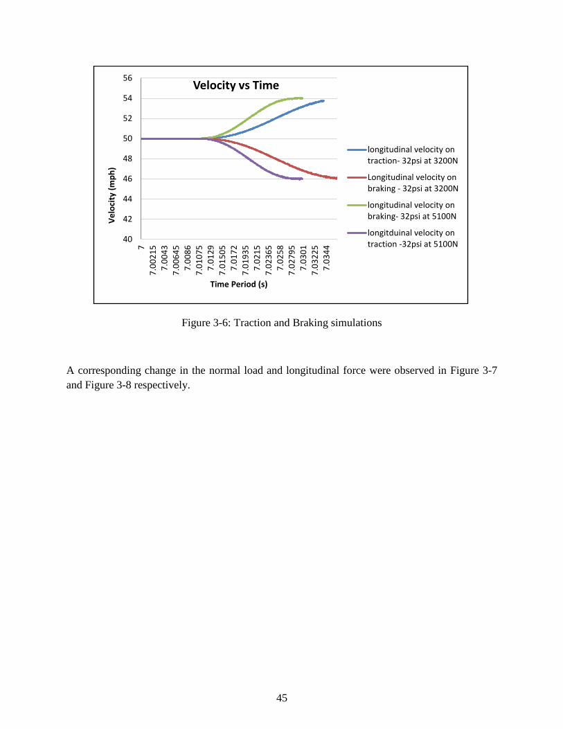
45

Figure 3-6: Traction and Braking simulations

A corresponding change in the normal load and longitudinal force were observed in Figure 3-7

and Figure 3-8 respectively.

40

42

44

46

48

50

52

54

56

7

7.0

02

15

7.0

04

3

7.0

06

45

7.0

08

6

7.0

10

75

7.0

12

9

7.0

15

05

7.0

17

2

7.0

19

35

7.0

21

5

7.0

23

65

7.0

25

8

7.0

27

95

7.0

30

1

7.0

32

25

7.0

34

4

Ve

loci

ty (

mp

h)

Time Period (s)

Velocity vs Time

longitudinal velocity ontraction- 32psi at 3200N

Longitudinal velocity onbraking - 32psi at 3200N

longitudinal velocity onbraking- 32psi at 5100N

longitduinal velocity ontraction -32psi at 5100N

46

Figure 3-7: Change in normal load for traction and braking cases

As seen in Figure 3-8 the longitudinal force varies by 1000 N when the load is 3200 N. The force

varies by 1500 N in when the load is 5100 N. Since the load is higher a larger tractive/braking

force is needed to reduce or increase the speed.

0

1000

2000

3000

4000

5000

6000

70007

7.0

01

75

7.0

03

5

7.0

05

25

7.0

07

7.0

08

75

7.0

10

5

7.0

12

25

7.0

14

7.0

15

75

7.0

17

5

7.0

19

25

7.0

21

7.0

22

75

7.0

24

5

7.0

26

25

7.0

28

7.0

29

75

7.0

31

5

7.0

33

25

7.0

35

Ne

t N

orm

al L

oad

(N

)

Time (s)

Normal Load vs Time

Net normal load on traction-32psi at 3922 N

Net normal load on braking- 32psi at 3922 N

Net normal load on traction-32psi at 5100 N

Net normal load on braking- 32psi at 5100 N

47

Figure 3-8: Change in Longitudinal force

Based on the above results we can state that the FE model is responding effectively to various

driving conditions.

3.9 Lateral force simulation.

The purpose of evaluating the lateral force generated by tires is to make a comparison of the

vehicle performance in dry and wet conditions. Based on the procedure mentioned in section 3.4

we can vary the slip angle as needed. One drawback of using *SST in Abaqus is the issue faced

with element distortion. At higher speeds and slip angles, the elements distort excessively which

can lead to convergence issues. Using *SST the simulation was run at a slip angle of 7ºhowever

the simulation failed to converge. For future work the speed can be reduced and higher slip angle

can be applied to investigate if the solution is converging, therefore the slip angle simulation was

limited to a slip of 5º. The lateral force generated by tires is evaluated at 3 different loads and 4

different slip angles. This force is then compared to identical conditions on wet surfaces.

Because the explicit FE simulations are computationally expensive, it is not feasible to run

different tests such as those run on a Flat Track Test rig. We have limited the slip angles

simulation so as to create a very simple vehicle dynamics model. If more time and resources

-2000

-1500

-1000

-500

0

500

1000

1500

2000

2500

7.0

00

05

7.0

01

75

7.0

03

45

7.0

05

15

7.0

06

85

7.0

08

55

7.0

10

25

7.0

11

95

7.0

13

65

7.0

15

35

7.0

17

05

7.0

18

75

7.0

20

45

7.0

22

15

7.0

23

85

7.0

25

55

7.0

27

25

7.0

28

95

7.0

30

65

7.0

32

35

Lon

gitu

din

al f

orc

e (

N)

Time Period (s)

Longitudinal force vs Time

Longitudinal force on braking- 32psi at 3200N

Longitudinal force ontraction- 32psi at 3200N

Longitudinal force on braking-32psi at 5100N

Longitudinal force ontraction- 32psi at 5100N

48

were available additional explicit simulations could have been carried out to attain more data so

as to create an effective vehicle dynamics model.

A constant water depth of 3 mm has been used for the explicit simulations for lateral force

generation since this represents typical conditions on water logged wet highways. The simulation

is initially run at a particular slip angle in *SST, this is then transferred to Abaqus/Explicit for

wet surface simulations. As the normal load acting on the tires reaches a steady state value the

corresponding lateral force generated by the tires also reaches a steady value. As such simulation

results are not readily available, test data obtained from a Calspan test rig was used to get an

estimate of the difference in lateral force generated on wet and dry surfaces.

NHTSA test data on Calspan for lateral force evaluation on wet surfaces has been made available

for research [49] . The test was carried out using Goodyear Eagle RSA P225/60R16 tires with

1.3 mm water depth. Figure 3-9 represents the results of the Calspan test on wet and dry surface.

It was observed that the lateral force on wet surfaces is typically lower by 300 N at low slip

angles. As slip angle increases the difference in the lateral force generated also increases. It was

also observed that the lateral force peaks at lower slip angle on wet surfaces as compared to dry

surfaces. This experimental test shows the basic trend of lateral force generated on wet and dry

conditions. Based on these test results a similar trend should be observed in the FE simulations.

It should be noted that the Calspan tests were conducted with an all season Goodyear Eagle tire

on a water depth of approximately 1.3 mm. The FE tire model has a different structure and the

water depth has been set to 3 mm. Using FE simulations setting a water depth of 1 mm will be

computationally expensive as an extremely fine mesh will be required.

Figure 3-9: Calspan test data, used under fair use [49]

Figure 3-10 shows the net load on the tires at various slip angles with an initial load of 3922 N. It

can be seen that a higher slip angle leads to a slight increase in the net load acting on the tires.

49

This can be attributed to the alignment of grooves and slots which at higher slip angles expel

water more efficiently.

Figure 3-10: Net Normal load at various slip angles- Load 3922 N

Figure 3-11 denotes the lateral force acting on the tires. The initial lateral force corresponds to

the force generated at the end of *SST. As the simulation in Abaqus/Explicit progresses the net

load acting on the tire goes down which leads to a change in the lateral force generation

capability of the tires.

0

1000

2000

3000

4000

5000

6000

9

9.0

01

8

9.0

03

6

9.0

05

4

9.0

07

2

9.0

09

9.0

10

8

9.0

12

6

9.0

14

4

9.0

16

2

9.0

18

9.0

19

8

9.0

21

6

9.0

23

4

9.0

25

2

9.0

27

9.0

28

8

Ne

t n

orm

al L

oad

(N

)

Time Period (s)

Net Normal Load vs Time

Net Load at 0 slip -3922 N

Net load at slip 2 degrees -3922N

Net load at slip 4 degrees-3922N

Net load at slip 5 degrees-3922 N

50

Figure 3-11: Lateral force acting at different slip angles- Load 3922 N

Based on literature [23, 50-52] it is observed that Abaqus/Explicit results tend to have noisy data

because of the nature of the dynamic simulations. Due to the small stable time increment used in

explicit dynamics, a lot of high frequency "noise" is associated with the signal (e.g., the ringing

associated with stress waves moving through the material and reflecting at boundaries). The

high frequency response is effectively damped out in implicit dynamics due to the larger time

steps used. When an incompressible medium is considered, these oscillations cannot stem from

compression effects. Abaqus, however, allows slight compressibility, which might be the source

of these oscillations [2]. To filter out these noise effects a Butterworth filter has been used with a

cutoff frequency of 100 Hz. This filtering process has been applied to both the normal load and

lateral force for each of the simulations. Steps have been taken to ensure that relevant data has

not been cutoff due to the filtering process. Figure 3-12 represents the filtered lateral force data.

The Butterworth filter is applied after a time step of 0.0015, when the tire starts rotating on the

water surface. As we are interested only in the final steady state solution the in-built Butterworth

filter in Abaqus provides an effective solution

0

500

1000

1500

2000

2500

3000

3500

4000

9

9.0

01

55

9.0

03

1

9.0

04

65

9.0

06

2

9.0

07

75

9.0

09

3

9.0

10

85

9.0

12

4

9.0

13

95

9.0

15

5

9.0

17

05

9.0

18

6

9.0

20

15

9.0

21

7

9.0

23

25

9.0

24

8

9.0

26

35

9.0

27

9

9.0

29

45

Late

ral f

orc

e (

N)

Time Period (s)

Lateral force vs Time

Lateral force at 0 slip

Lateral force at 2 degree slip



51

Figure 3-12: Filtered lateral force data

The process is repeated for a load of 3200 N and 5100 N to transfer the data to CarSim for a

vehicle dynamics model.

Figure 3-13: Net Normal load at various slip angles- Load 3200 N

0

500

1000

1500

2000

2500

3000

9.0

01

69

.00

33

99

.00

51

79

.00

69

69

.00

87

49

.01

05

39

.01

23

19

.01

41

9.0

15

88

9.0

17

67

9.0

19

45

9.0

21

24

9.0

23

02

9.0

24

81

9.0

26

59

9.0

28

38

Late

ral F

orc

e (

N)

Time Period (s)

Filtered Lateral Force Data

Lateral force at zero slip

Lateral force at 2 degreeslip



0

500

1000

1500

2000

2500

3000

3500

4000

4500

9

9.0

01

8

9.0

03

6

9.0

05

4

9.0

07

2

9.0

09

9.0

10

8

9.0

12

6

9.0

14

4

9.0

16

2

9.0

18

9.0

19

8

9.0

21

6

9.0

23

4

9.0

25

2

9.0

27

9.0

28

8

Ne

t n

orm

al L

oad

(N

)

Time Period (s)

Net Normal Load vs Time

Net Load at 0 slip -3200N

Net load at slip 2 degrees -3200N



52

As observed in Figure 3-13 various oscillations are observed in the beginning of the time step.

This can be attributed to the transfer of the contact state to Abaqus/Explicit. These oscillations

occur only at higher slip angles where the elements tend to be distorted. The oscillations fade out

towards the end of the simulation hence they won’t have a major influence on the final steady

state solution.

Table 3-3 shows the lateral force data at a load of 3922 N and various slip angles. The lateral

force at zero slip angle can be attributed to the ply steer effect. As the slip angle increases the

difference in lateral force on wet and dry surfaces increases. It can be seen that at a slip angle of

5º, on dry surface, the peak lateral force has not been attained, whereas on the wet surface the

peak lateral force has almost been achieved at 5º slip. This is similar to the data published based

on the Calspan tests [53].

Table 3-3: Lateral force data at a load of 3922 N

Load on Tire

at the end of

*SST

Slip applied

at *SST

Final load on tire (end

of explicit

hydroplaning)

Lateral force

(End of *SST)

Final Lateral force

(End of explicit

hydroplaning)

Initial Load

(N)

Lateral slip

(deg)

Final Load (N) Initial Lateral

Force (N)

Final Lateral Force

(N)

3922 0 2140 85 84

3922 2 2403 1877 1304

3922 4 2530 2654 1600

3922 5 2443 2854 1617

Figure 3-14 draws a comparison between the lateral force data on wet and dry surface based on

the FE siulations. If several data points at higher slip angle were available the trend would be

similar to Calspan test data. However since excessive element distortion occurs at higher slip

angles this is not a feasible solution. Also FE simulations are extremely time consuming, to limit

the scope of the project only 4 slip angles have been considered.

53

Figure 3-14: Lateral force comparison- Load 3922 N

Similar slip angle data has been evaluated for a load of 5100 N and 3200 N. The trend observed

is similar for all 3 cases. Figure 3-15 and Table 3-4 represent the simulation data at a load of

3200 N. It can be noted that at a load of 3200 N the lateral force generated on the dry surface is

also nearing its peak limit. This is similar to the trend observed in several experimental tests,

where the lateral force peaks quickly at lower slip angles for lower loads as compared to higher

loads.

0

500

1000

1500

2000

2500

3000

0 2 4 5

Late

ral F

orc

e (

N)

Slip angle (Deg)

Lateral Force vs Slip Angle at 3922 N

Lateral Force on Wetsurface

Lateral Force on Drysurface

54


Load on Tire

at the end of

*SST

Slip applied

at *SST


of explicit

hydroplaning)

Lateral force

(End of *SST)

Final Lateral force

(End of explicit

hydroplaning)

Initial Load

(N)

Lateral slip

(deg)


Force (N)

Final Lateral Force

(N)

3200 0 1610 77 77

3200 2 1652 1659 880

3200 4 1760 2264 1052

3200 5 1785 2394 1060


Table 3-5 and Figure 3-16 represent the simulation data at a load of 5100 N. It can observed that

contrary to the lateral force data at a load of 3200 N the lateral force has not yet peaked even at a

0

500

1000

1500

2000

2500

3000

0 2 4 5

Late

ral F

orc

e (

N)

Slip angle (Deg)




55

slip angle of 5 degrees, thus confirming that the FE model results are comparable to experimental

data.


Load on Tire

at the end of

*SST

Slip applied

at *SST


of explicit

hydroplaning)

Lateral force

(End of *SST)

Final Lateral force

(End of explicit

hydroplaning)

Initial Load

(N)

Lateral slip

(deg)


Force (N)

Final Lateral Force

(N)

5100 0 3171 90 114

5100 2 3524 2185 1631

5100 4 3578 3116 2147

5100 5 3614 3543 2419


With the given lateral force data on wet and dry surface we can now create a simple Pacejka

model or use CarSim for vehicle dynamics simulations. Based on the results obtained it is

0

500

1000

1500

2000

2500

3000

3500

4000

0 2 4 5

Late

ral F

orc

e (

N)

Slip Angle (Deg)




56

evident that the wet surface, as it has a lower lateral force generation capability, will have less

traction capability. Both the Pacejka model and the in-built CarSim tire modeling method have

been evaluated for this research. However the Pacejka model curve fit will require lateral force

measurements at several slip angles and camber angles. This is not feasible given the

computation time taken for the FE simulations. Therefore the in-built tire modeling feature in

CarSim has been used as an alternative. Although the data set is not large enough to represent

several driving conditions and accurately describe the non-linear operating range of the tires, it is

sufficient to develop a simple vehicle dynamics model. Figure 3-17 denotes the expected

hydroplaning speed on a water depth of 3mm at loads of 3922 N and 3200 N. This result will be

used for vehicle dynamics simulations.

Figure 3-17: Expected Hydroplaning speed on water depth of 3 mm.

57

4 CarSim Vehicle Dynamics Simulations

CarSim is one of the most famous vehicle dynamics simulation programs. It is the preferred

program for analyzing vehicle dynamics, developing active controllers, calculating a vehicle’s

performance characteristics, and developing active safety systems. Typical vehicles of different

classes (e.g., passenger car, SUV, heavy truck), road characteristics and driver behavior can be

modeled in a relatively short time. Also more detailed tire models can be used via external

programs such as MATLAB/Simulink [54-62].

To get an understanding of the difference in tire traction capabilities on wet and dry surfaces,

several tests were run on CarSim. Based on the FE simulation expected hydroplaning speed for

the given tread pattern at a load of 3922 N and water depth of 3mm is above to 60 mph. But this

does not take into account the dynamics of the car. The dynamics of a single tire is taken into

account. When the Lateral force data is incorporated into CarSim the lookup table generates a

force VS slip angle plot for the tires. Figure 4-1and Figure 4-2 denote the plots based on the

lookup table generated by CarSim.

Figure 4-1: CarSim lateral force data on Dry surface

58

Figure 4-2: CarSim lateral force data on Wet surface

A Class C hatchback car was used for the simulation. A tire closely representing the FE tire

model was selected. In CarSim a175/65R14 tire was selected for the simulation. The Car has a

mass of 1250 kg which is equivalent 12300N. This is comparable to the case where the tire has a

load of 3200 N in the FE simulations. It was observed that the hydroplaning speed for such a

condition at a water depth of 3mm was close to 57 mph. For the Constant Radius test, CarSim

will take into account a water depth of 3mm and all four tires of the vehicle will have the same

amount of grip. This will have a significant impact on the stability and hydroplaning speed of the

vehicle.

4.1 ISO 4138 Constant-Radius Test

Understeer gradient is a measure of how the steering needed for a steady turn changes as a

function of lateral acceleration. Steering at a steady speed is compared to the steering that would

be needed to follow the same circular path at very low speed; this is called the Ackermann steer

angle. The vehicle has a positive understeer gradient if the difference between required steer and

the Ackermann steer increases with respect to incremental increases in lateral acceleration; it has

a negative gradient if the difference in steer decreases with respect to lateral acceleration. A

vehicle is said to understeer when the understeer gradient is positive; a vehicle is said to

oversteer when the gradient is negative; a vehicle is said to have neutral steer when the gradient

is zero.

59

Several tests can be used to determine understeer gradient: constant radius (repeat tests at

different speeds), constant speed (repeat tests with different steering angles), or constant steer

(repeat tests at different speeds). The Ackermann angle remains constant when the constant

radius method is used, and the gradient of steering wheel angle with respect to lateral

acceleration is therefore a valid measure of understeer gradient in this specific test [63].

ISO 4138 describes several methods for generating plots of steering VS. Lateral acceleration.

This simulation covers the constant-radius test made with slowly increasing speed. In this test,

the vehicle is driven at a low speed around a circular path; when the response has settled, the

observed steering wheel angle is defined as the Ackermann angle for the path radius. The

understeer behavior is then determined by driving with a slowly increasing speed, with the

restriction that the rate at which lateral acceleration increases must be limited to 0.1 (m/s2) [63].

The speed control is initially set using the built-in closed-loop controller, with target speed set as

a function of time. The target speed is initially 6 km/h. No open-loop braking is applied. Shifting

is performed with a closed-loop controller that will use the shift schedules for the vehicle, using

all gears available in the vehicle. Steering is set with a closed-loop path follower that will follow

the target path (road centerline) using a 0.25 second preview time (tight path tracking) and a low-

speed limit.

In the constant understeer 100 m radius tests, the simulation is started with an initial velocity of 6

km/h. The simulation is set up such that all 4 tires of the car are either wet or dry. Although

these parameters will not be completely applicable in real world simulations, conditions can be

altered such that the front two tires are wet followed by dry rear tires. The constant understeer

test is run such that the vehicle reaches a velocity of 50 km/hr and 75 km/hr; various responses

are then evaluated using CarSim.

4.1.1 Results at 50 km/hr

We can see that at a speed of 50 km/hr, the dry surface lateral force data induces understeer

characteristics in the car. With the wet surface force data the vehicle has similar understeer

characteristics. From Figure 4-3 we can see that a lateral acceleration of 0.2 g is generated at 50

km/hr. On the dry surface the vehicle still has the ability to generate more lateral force, however

with all four tires moving on the wet surface at a water depth of 3 mm, the tires generate less

force thus the steering angle is increased towards the end of the simulation. This can be

attributed to the fact that on the wet surface based on the FE simulations results, the vehicle

lateral forces peak very quickly. As the number of extrapolation points based on the FE

simulation provided to CarSim are extremely low, the results obtained using CarSim will not be

as smooth as the results obtained by incorporating experimental tire test data at several slip

angles and loads. Similar results can also be seen in Figure 4-4.

60

Figure 4-3: Steering wheel angle vs. Lateral acceleration- Speed 50 km/hr

Figure 4-4: Steering wheel angle vs. Time- Speed 50 km/hr

61

Vehicle Sideslip Angle

When a car is driven straight on a flat surface, the direction of travel at the center of gravity (CG)

remains the same as the orientation of the vehicle (that is, the direction of the longitudinal axis).

When the car turns, however, it exhibits a yaw rate, causing the orientation to change, and a

lateral acceleration directed toward the center of the turn. The car also exhibits a velocity

component perpendicular to the orientation, known as the lateral velocity, means that the

orientation of the vehicle and the direction of travel are no longer the same. The lateral velocity

differs from one point on the vehicle body to another; as a point of reference, we use the

vehicle’s CG. The angle between the orientation of the vehicle and the direction of travel at the

CG is called the vehicle sideslip angle [64]. Under normal circumstances, when the car is driven

safely without danger of losing road grip, the vehicle sideslip angle is small, not exceeding 2ºfor

the average driver.

From Figure 4-5 can see that on the wet surface the side slip is decreasing rapidly as the speed

increases showing an apparent loss in stability. Steering and side slip angle can be used as

indicators of vehicle stability as they can be used to characterize the understeer and oversteer

tendency of a vehicle. Similar tests are carried out at a speed of 75 km/hr.

Figure 4-5: Vehicle side slip angle vs. Time – Speed 50 km/hr

4.1.2 Results at 75 km/hr

As mentioned in the previous section all 4 tires have the same lateral force generation capability

on wet surface. This is not necessarily an accurate representation of real world driving conditions

62

as typically in modern passenger cars the front tires expel majority of water thus paving a clear

path for the rear tires. Also with the given simulation we are assuming that the water depth is

3mm throughout the understeer test which affects the vehicle stability on wet surface. From

Figure 4-6 we can see that on the wet surface the vehicle starts oversteering when the lateral

acceleration reaches 0.32 g in the specified conditions. As the peak force generation capacity of

the tires at a particular dynamic load and slip angle is reached, the driver increases his steering

angle to maintain the optimal path. However, above 0.3 g the car starts oversteering and the

driver reduces the steering input to maintain control over the vehicle. As observed in Figure 4-6

on a water depth of 3 mm the vehicle starts losing stability close to 0.3 g, whereas the car is still

stable on the dry surface.

Figure 4-6: Steering wheel angle vs. Lateral Acceleration- Speed 75 km/hr

From the sideslip angle data in Figure 4-7 we can see that on the wet surface the car has lost

traction and the side slip angle has reached -5 º. This indicates that the rear of the car has a much

greater slip angle as compared to the front causing the car to sway, leading to a loss of vehicle

stability.

63

Figure 4-7: Vehicle side slip angle vs. Time – Speed 75 km/hr

From Figure 4-8 we can compare the vehicle position at the same time step during the

simulation. As we can see on the dry surface the vehicle is able to follow the optimal path but on

the wet surface where the traction is lower the vehicle oversteers.

Figure 4-8: Vehicle position at identical times (t=31 s)

64

Vehicle response has also been evaluated when only the front tires are wet. From Figure 4-9 we

observe that in this case the car exhibits an increasing understeer tendency on the wet surface

where the front tire slip angles are greater than the rear. Hence the steering angle increases.

Based on such variations we can state that to create an accurate hydroplaning model, actual

conditions have to replicated in CarSim based on experimental tests. However, such data is

currently not available.

Figure 4-9: Steering wheel angle vs. Lateral acceleration- Wet front tires- Speed 75 km/hr

From Figure 4-10 we can see that the vehicle side slip angle is similar for both dry and wet

conditions indicating that the vehicle is still under control and in the stable operating region.

65

Figure 4-10: Vehicle side slip angle vs. Time – Wet front tires- Speed 75 km/hr

4.1.3 Comparison of FEA results with Calspan Test Data

The Calspan lateral force test data [53] on wet and dry surfaces has been used to evaluate

stability in CarSim. This can be used to compare the FE results against an actual experimental set

up. As this test has been conducted at a lower water depth and using a larger tire with a different

groove depth, the lateral forces generated are higher and also peak slower as compared to the FE

results. However, it is observed that close to a lateral acceleration of 0.45 g the vehicle loses

stability and starts oversteering. This is similar to the results obtained based on the FE

simulation.

66

Figure 4-11: Lateral force based on Calspan test data [53]

As shown in Figure 4-12 the vehicle side slip reaches -10 º which indicates that the car is

deviating from the optimal path and is also oversteering. This is similar to the simulation

performed based on the FEA Results. Based on these results we can state that during the course

of an understeer test on wet surface, the vehicle starts losing stability beyond 0.4 g of lateral

acceleration.

67

Figure 4-12: Vehicle Side Slip angle based on Calspan Data

4.2 Double lane change (DLC) at 120 km/hr The double lane change maneuver can be used to evaluate vehicle performance seen in everyday

driving conditions. Figure 4-13 and Figure 4-14 compare the vehicle positions in CarSim during

the DLC maneuver at identical time steps.

Figure 4-13: DLC on dry surface

68

Figure 4-14: DLC on wet surface

At the same instant, on the wet surface the vehicle is unable to follow the ideal lane change path

and is slowly losing control. The rear tires are slipping more than the front tires indicating an

oversteer tendency and lack of grip. With the dry surface data the car is almost following the

ideal lane change path whereas using the wet surface data the driver almost loses control of the

car. Figure 4-15 shows the steering wheel input for the lane change maneuver. It can be seen that

the driver has to increase his steering input to maintain control over the vehicle on wet surface.

This depicts the possibilities of accidents occurring on water logged highways. Such tests can be

used to evaluate vehicle stability on wet roads and can provide valuable inputs to both pavement

design engineers and automotive companies to devise new methods to enhance vehicle stability.

69

Figure 4-15: Steering wheel angle vs Time- DLC

Figure 4-16 shows the optimal patch to be tracked by the vehicle for the DLC maneuver. We can

see on the dry surface the vehicle is able to track the optimal path efficiently whereas on wet

surface the patch tracking error increases by 2 meters. Based on Figure 4-15 one can note, to

maintain optimal path on the wet surface the driver has to vary his steering input rapidly, this

may lead to accidents in real world driving conditions.

70

Figure 4-16: Vehicle Path Tracking

4.2.1 Comparison of FEA results with Calspan Data - DLC

Similar to the FEA results, based on Figure 4-17 and Figure 4-18 we can see that the driver has

to make rapid changes to his steering input to follow the optimum path on the wet surface. This

shows that the FE results show trends similar to the Calspan data. Based on these results we can

state that hydroplaning FSI simulations can play a vital role in tread design development as they

can be used to evaluate tire performance before a test tire has been built.

71

Figure 4-17: Steering wheel angle vs Time- DLC- Calspan data

Figure 4-18: Vehicle Path Tracking- Calspan data

72

5 Conclusion and future work

The main goal for this research is to develop a firm understanding of the physics of hydroplaning

taking into consideration various tire design parameters and vehicle configurations. This research

has investigated a method to develop a simple vehicle dynamics model based on FE simulations.

Vehicle stability has been deduced based on several standard tests in CarSim. The feasibility of

Abaqus FSI to develop a single tire hydroplaning simulation has been evaluated. Based on the

FSI results we can conclude that the Abaqus CEL approach is an effective tool to study the

influence of various tread patterns on hydroplaning velocity. This can be utilized by tire

researchers to enhance the tread design parameters for wet surfaces. The CEL approach can also

be used to evaluate the effectiveness of a given tread pattern at different water depths. A huge

drawback of Abaqus/Explicit is the computational time involved in such complex FSI

simulations. Also, Abaqus elements tend to distort at high slip angles and speeds making it

difficult to evaluate tire response at such configurations. This limits the use of Abaqus to develop

a Pacejka model based on which accurate vehicle dynamics simulations can be carried out.

Although Abaqus will help tire design researchers to study the influence of fundamental tire

designs, it will be easier to use a Flat Track test rig incorporated with a test set-up to generate

wet surfaces to compare tire performance on wet and dry surfaces. With such a set-up it will be

easier to evaluate the difference in tire performance at several slip angles, camber angles and

water depths. Based on the simple vehicle dynamics model developed in CarSim it was observed

that the vehicle operates in a highly unstable region on wet surfaces. Lack of traction due to the

low lateral force generation capacity on wet surfaces leads to a decrease in grip, thereby causing

the rear tires to slip thus resulting in a oversteer tendency. In both the Constant Radius test and

DLC test, the driver had to either reduce his steering input or at times increase the steer angle to

maintain control over the vehicle on the wet surface. The DLC maneuver illustrates the issues

that can be faced in real world driving conditions. However due to availability of limited data

points based on the FE simulations, results will not be as accurate as those obtained when tire

force data based on experimental testing is used in CarSim. As observed in the Section 4.2, the

driver was unable to maintain the optimal lane change path; this can prove to be a fatal incident

on several highways.

Based on the results of the thesis, we can confidently state the Abaqus FSI can be used to study

influence of tire design parameter on hydroplaning velocity. The FSI results show trends similar

to the Calspan test data. Abaqus FSI can be used to study several tire tread pattern performances

on wet surfaces before an actual test pattern is developed. If a real world tire model was made

available for academic research by tire manufacturers, a comparison between the FE simulation

73

and experimental tests can be made by using sensor embedded intelligent tires. In this way a true

validation of Abaqus FSI for hydroplaning can be carried out by academic institutions. This can

also help to develop control algorithms to maintain vehicle stability on wet surfaces. This study

opens a new area of research and invites researchers and engineers to work on it. There are

several improvement opportunities that one should think of. Future researchers can extend the

work to develop a robust hydroplaning vehicle dynamics model. Future work can involve the

following:

Evaluate the influence of several fundamental tire designs and find an appropriate pattern

which can be used for wet driving conditions however this is subject to availability of

more computing resources and Abaqus/Explicit license tokens

Extend slip angle iterations to find tire performance at higher slip angles and loads so as

to develop a Pacejka Model.

Researchers can develop a separate Pacejka model for each fundamental tread pattern and

use it in a vehicle dynamics model.

Obtain real world tire model readily available in the market to correlate FSI simulations

with experimental tests using intelligent tires.

74

6 References

1. Gisper, M. FTire, a new fast tire model for ride comfort simulations. in International ADAMS User’s Conference Berlin. 1999.

2. Sillem, A., Feasibility study of a tire hydroplaning simulation in a monolithic finite element code using a coupled Eulerian-Lagrangian method, in Delft Institute of Applied Mathematics. 2008, Delft University of Technology: Delft, the Netherlands.

3. Fwa, T.F., Kumar. A., Ong, G.P., Relative effectiveness of grooves in tire and pavement in reducing vehicle hydroplaning risk. Transportation Research Record, 2010. 2155: p. 73-81.

4. Okano, T., and Koishi, M.,. Hydroplaning Simulation using MSC. Dytran. in Proceedings of the 3rd European LS-DYNA Users Conference. 2001. Paris, France.

5. Taheri, S., Tire Mechanics Lecture Notes Virginia Tech. Spring 2013. 6. Terry, D., A simulation model for vehicle braking systems fitted with ABS,

in SAE world congress. 2002: Michigan. 7. Allbert, B.J., Tires and Hydroplaning. SAE Paper 680140, 1968. 8. Sinnamon, J.F., Hydroplaning and tread pattern hydrodynamics, in

Highway safety research institute/ University of Michigan. 1974. p. 132. 9. Horne, W.B., and Dreher, R. C. Phenomena of Pneumatic Tire

Hydroplaning. in National Aeronaustics and Space Administration. 1963. Washington D.C.

10. Horne, W., Yager, T. and Taylor, G, Review of Causes and Alleviation of Low Tire Traction on Wet Runways. 1968: NASA Technical Note.

11. Horne, W.B., Yager, T.J and Iveyd.L, Recent studies to investigate effects of tire footprint aspect ratio on dynamic hydroplaning speeds. American society for testing and material, 1986. ASTM STP 929: p. 26-46.

12. Gengenbach, W., Experimental investigation of tires on wet pavements, in Automotive technology magazine. 1968. p. 70, 83-89, 288-293, 310-316.

13. Gallaway, B.M., Pavement and Geometric Design Criteria for Minimizing Hydroplaning, in Report No. FHWA-RD-79-31. 1979, Texas Transportation Institute: Federal Highway Administration.

14. Mounce, J.M., Hydroplaning and roadway tort liability. Transportation Research Record, 1993(1401): p. 117.

15. Cerezo, V., Gothie, M., and Menissier, M. , Hydroplaning speed and infrastructure characteristics. Proceedings of the Institution of Mechanical Engineers, 2010. 224(J9): p. 891.

75

16. Agarwal, S.K., Braking Performance of Aircraft Tires. Prog. Aerospace Sci, 1986. Vol. 23: p. 105-150.

17. Yager, T., Phillips, W.P. and Hore, W., A Comparison of Aircraft and Ground Vehicle Stopping Performance on Dry, Wet, Flooded, Slush, Snow, and Ice Covered Runways. 1970: NASA Technical Note.

18. Seta, E., Nakajima, Y., Hydroplaning analysis by FEM and FVM: effect of tire rolling and tire pattern on hydroplaning. Tire Sci. Technol., 2000. 28(3): p. 140-156.

19. Okano, T., Koishi, M. , A new computational procedure to predict transient hydroplaning performance of a tire. Tire Sci. Technol., 2001. 29(1): p. 2-22.

20. Bathe, K.J., Zhang, H., Finite Element Developments for General Fluid Flows with Structural Interactions. International journal of numerical methods in Engineering, 2004. 60: p. 21-32.

21. Cho, J.R., Lee, H. W., Numerical Investigation of Hydroplaning characteristics of Three-dimensional patterned tire. European Journal of Mechanics A/Solids, 2006. 25(6): p. 914-926.

22. Cho, J.R., Lee, H. W., A wet-road braking distance estimate utilizing the hydroplaning analysis of patterned tire. International journal of numerical methods in Engineering, 2007. 69: p. 1423-1445.

23. Kim, T.W., Jeong, H.Y. , Hydroplaning simulations for tires using FEM, FVM and an asymptotic method. International journal of automotive technology, 2010. 11(6): p. 901.

24. Vincent, S., Sarthou, A., Augmented Lagrangian and penalty methods for the simulation of two-phase flows interacting with moving solids. Application to hydroplaning flows interacting with real tire tread patterns. Journal of computational physics, 2011. 230: p. 956-983.

25. Wang, H., Imad L., Al-Qadi, Simulation of tyre-pavement interaction for predicting contact stresses at static and various rolling conditions. International journal of Pavement Engineering, 2012. 13: p. 310-321.

26. Ong, G., Fwa, T. F., Transverse pavement grooving against hydroplaning, I: simulation model. Journal of Transportation Engineering, 2006. 132(6): p. 441-448.

27. Ong, G.P., Fwa,T.F., Kumar, A., Transverse pavement grooving against hydroplaning. II: Design. Journal of Transportation Engineering 2006. 132: p. 449-457.

28. Ong, G.P., Fwa, T. F., Part 3: Pavement Surface Properties-Vehicle Interaction: Analysis of Effectiveness of Longitudinal Grooving Against

76

Hydroplaning. Transportation Research Record: Journal of the Transportation Research Board, 2006(1949): p. 113-125.

29. Srirangam, S.K., Anupam, K. , Study of Hydroplaning Risk on Rolling and Sliding Passenger Car. Procedia - Social and Behavioral Sciences, 2012. Volume 53: p. 1019–1027.

30. Ong, G.P., Fwa, T. F., Effectiveness of transverse and longitudinal pavement grooving in wet-skidding control. Transportation Research Record: Journal of the Transportation Research Board., 2007(2005): p. 172-182.

31. Ong, G.P., Fwa, T. F., Modeling and analysis of truck hydroplaning on highways. Journal of the Transportation Research Board, 2008(2068): p. 99-108.

32. Gunaratne, M. and Q. Lu, Hydroplaning on Multi Lane Facilities. 2012: Florida department of transportation.

33. Allberts, B.J., Walker, J.C., Tyre to Wet Road Friction at high speeds. Proc Institution of Mechanical Engineers, 1965-66. Vol 180.

34. Maycock, G., Experiments on Tyre Tread Tatterns. Vol. LR 122. 1967: Road Research Laboratory Report. 25.

35. Horne, W.B., Joyne, U. T. . Pneumatic tire hydroplaning and some effects on vehicle performance. in SAE International Automotive Engineering Congress. 1965. Detroit, Michigan, USA.

36. Lee, K.S., Effect of sipes on viscous hydroplaning of Pneumatic Tires. Tire Science and Technology, 1998. 26(1): p. 23-35.

37. Fwa, T.F., Kumar, A., and Ong, G. P. , Effectiveness of Tire-Tread patterns in Reducing the Risk of Hydroplaning. Transportation Research Record: Journal of the Transportation Research Board, 2009. 2094.

38. Cho, J.R., Kim, K.W.,, Mesh Generation Considering Detailed Tread Blocks for Reliable 3D Tire Analysis. Advances in Engineering Software, 2004. 35: p. 105-113.

39. Korunovic, N., Detailed vs. Simplified Tread Tire Model for Steady-State Rolling Analysis. Journal for Theory and Application in Mechanical Engineering, 2012. 54: p. 153-160.

40. Wies, B., Roeger, B., Influence of Pattern Void on Hydroplaning and related Target Conflicts. Tire Science and Technology, 2009. 37(3): p. 187-206.

41. Metz, L., Hydroplaning behaviour during Steady- State Cornering. SAE International Journal of Materials and Manufacturing, 2011. 4: p. 1068-1079.

77

42. Donea, J., Arbitrary Lagrangian–Eulerian Methods. Encyclopedia of Computational Mechanics, NOV 2004.

43. Simulia, Abaqus 6-13 User Manual. 44. Ong, G.P., Fwa, T. F., Prediction of wet-pavement skid resistance and

hydroplaning potentioal. Journal of the Transportation Research Board, 2007: p. 160-171.

45. Ong, G.P., Fwa, T. F., Wet-pavement hydroplaning risk and skid resistance: modeling. Journal of Transportation Engineering, 2008. 133(10): p. 590-598.

46. Ong, G.P., Fwa, T. F., Modeling hydroplaning and effects of pavement microtexture. Transportation Research Record: Journal of the Transportation Research Board, 2005(1905): p. 166-176.

47. Ong, G.P., Hydroplaning and skid resistance analysis using numerical modeling, in Department of Civil Engineering. 2006, National University of Singapore.

48. Donatellis, M., Virtual Treaded Tire Simulation as a Design Predictive Tool: Application to Tire Hydroplaning, in 2009 SIMULIA Customer Conference. 2009.

49. Salaani, M., Measurement and Modeling of Tire Forces on a Low Coefficient Surface in SAE World Congress. 2006.

50. Vincenzo D'Alessandro, Phenomenological analysis of hydroplaning through intelligent tyres. Vehicle System Dynamics: International Journal of Vehicle Mechanics and Mobility, 2012. 50: p. 3-18.

51. Walhorn, E., Hübner, B., Space‐Time Finite Elements for Fluid‐Structure Interaction. PAMM, 2002. 1(1): p. 81-82.

52. Matthies, H.G., Steindorf, J., Partitioned strong coupling algorithms for fluid–structure interaction. Computers & Structures, 2003. 81(8): p. 805-812.

53. Salaani, M.H., G, Measurement and Modeling of Tire Forces on a Low Coefficient Surface. SAE International, 2006.

54. MSC, CARSIM: Math Models. . 2014, Mechanical Simulation Corporation. 55. MSC, CarSim 9.0 Improvements. . 2014, Mechanical Simulation

Corporation. 56. MSC, CarSim Educational User Reference Manual. . 1998, Mechanical

Simulation Corporation. 57. Sengupta, A., Evaluating the effectiveness of collision avoidance functions

using state-of-the-art simulation tools for vehicle dynamics. 2013, Royal Institute of Technology.

78

58. Sendur, P., Thibodeau, R. Development & validation of a generic 3-D vehicle model & GUI for studying the handling performance. in Virtual Product Development Conference. 2004.

59. Eriksson, J., Nybacka, M., Larsson, T., and Lindgren, P. . Using Timber in a multi-body design environment to develop reliable embedded software. in SAE World Congress. 2008.

60. Sayers, M., Vehicle models for RTS applications. Vehicle System Dynamics., 1999.

61. Jamg, B., Study on concurrent simulation technique of Matlab CMDPS and a CarSim base full car model. Journal of the Korea Academia-Industrial Cooperation Society., 2013.

62. NI, Using simulation models with NI VeriStand. 2014, National Instrument.

63. MSC, Making Advanced Procedures with Vs Commands. 2011. 64. Grip, H.I., L, Vehicle Sideslip Estimation: Design, implementation, and

experimental validation, in IEEE CONTROL SYSTEMS MAGAZINE.

Developing a Vehicle Hydroplaning Simulation using Abaqus ... · v 2.10.3 Influence of tire sipes...

Documents

Transcript of Developing a Vehicle Hydroplaning Simulation using Abaqus ... · v 2.10.3 Influence of tire sipes...