1

Determinants of Firm Level Technical Efficiency: A Stochastic

Frontier Approach* Evis Sinani** and Derek C. Jones and Niels Mygind Revised February 21, 2007 Abstract By using an empirical approach seldom used in this area for transition economies (namely, stochastic frontiers) we investigate the determinants and dynamics of firm efficiency. This approach allows us to simultaneously estimate the parameters of both the efficiency and the production function. We also use most unusual data --a representative sample of Estonian firms for the period 1993-1999 – and are able to address problems that plague much previous work, such as the endogeneity of ownership. Consequently our findings are more reliable and efficient than most previous estimates. Our main findings are that: (i) compared to employee and state ownership, foreign ownership increases technical efficiency; (ii) firm size and higher labor quality enhance efficiency, while soft budget constraints adversely affect efficiency; (iv) Estonian firms operate under constants returns to scale; (v) the percentage of firms operating at high levels of efficiency increases over time. As such our findings provide support for hypotheses that a firm’s ownership structure and its characteristics are important for its technical efficiency. Keywords: Stochastic Frontier, Technical Efficiency, Transition, Soft Budget

Constraints and Ownership Structure. JEL Classification: C33, D21, D24, G32, J54, L25. *The paper has benefited from comments from participants at several presentations including: the 2nd Hellenic Workshop on Measurement of Efficiency and Productivity Analysis, in Patras, Greece, in 2003; the 4th Conference Enterprise in Transition in Spilt, Croatia 2003; the 29th European International Business Association Annual Conference in Copenhagen, in 2003; and a seminar at Hamilton College, 2005. **Evis Sinani, the corresponding author, is at the Department of International Economics and Management, Copenhagen Business School, Porcelaenhaven 24, 2000 Frederiksberg, Denmark: email: es.cees@cbs.dk. Derek C. Jones is at the Department of Economics, Hamilton College, Clinton, NY 13323, USA: email: djones@hamilton.edu. Niels Mygind is at the Department of International Economics and Management, Copenhagen Business School, Porcelaenhaven 24, 2000 Frederiksberg, Denmark: email: nm.cees@cbs.dk.

2

1. Introduction

The privatization process in transition economies has resulted in the emergence of a

variety of ownership structures and has also generated an extensive theoretical debate over

which form of private ownership would lead to better restructuring outcomes and higher

efficiency levels. This theoretical literature concludes that certain ownership forms are

preferred, in particular that outsider ownership is expected to be more efficient than insider

ownership (Aghion and Blanchard, 1998). There is also an extensive empirical literature for

transition economies, which assesses the effects of different ownership structures on

enterprise performance and efficiency. In a comprehensive literature review of that literature,

an influential survey by Djankov and Murrell (2002) concludes that, in general, privatization

will improve firm performance so that privatized firms will perform better than state owned

firms and that concentrated ownership is beneficial for firm performance. They also find that

Central and Eastern European countries experienced a larger positive impact of privatization

than did CIS countries.

At the same time, as Djankov and Murrell (2002) themselves note, the empirical

literature on firm performance and privatization has faced formidable estimation challenges

and thus most conclusions are necessarily tentative. Of central importance are issues related

to the endogeneity of ownership structures, for example the view that often insiders selected

the best performing firmsi. Several studies find that empirical findings are quite sensitive to

attempting to deal with endogeneity problems. In the main studies that grapple seriously with

endogeneity find that outsider ownership improves firm performance more than insider

ownership (e.g. Earle and Estrin, 1997). Also studies find that particular types of outsider

ownership work best. Thus Smith, Cin and Vodopivec (1997) find that foreign ownership

improves firm performance most in Slovevia while Frydman et al., (1999) conclude that firms

that are owned by domestic outsiders perform slightly better than foreign owned firms. But

not all studies that attempt to deal with endogeneity find that all forms of outsider ownership

3

have a large performance edge over all forms of insider ownership (e.g. Jones and Mygind,

2003, for Estonian frims).

In addition other authors have also drawn attention to other difficulties confronting

empirical work in this area and, as a result, do not always reach conclusions comparable to

those of Djankov and Murrell. For instance, Bevan, Estrin and Schaffer (1999) and Filer and

Hanousek (2001) point out that problems related to differences in accounting standards often

undermine the credibility of performance variables. Another problem is that many studies

may have used the most reliable empirical strategies and that much empirical work may have

neglected key issues such as the dynamics of efficiency. Finally, confidence in the reliability

of general findings in this field is undermined by the fact that often data samples have been

small and not representative.

This paper attempts to respond to these empirical challenges and is distinguished form

much previous work in several respects. First, our data are a long and rich panel for a sample

of firms that is representative of the Estonian economy and including firms with diverse

ownership structures. Second, these data and the technical approach we employ enables us to

estimate the impact on the level of firm technical efficiency of several crucial variables,

including ownership structures, soft budget constraints and competition. Third, the long time

horizon in our data enables us to account for the issue of endogeneity, in a more thorough

way than in many other earlier studies. Fourth, our modeling strategy permits us to

distinguish between shifts in the production function and changes in technical inefficiency

over time. Finally, and most unusually, we examine aspects of the dynamics of efficiency,

including presenting evidence of the distribution of efficiency scores over time and across

firms with various ownership structures.

The structure of the paper is as follows. In section 2, we discuss the determinants of firm

efficiency. In the following two sections the privatization process in Estonia is first outlined

and then we discuss our data. This is followed in section 5 by a discussion of the estimation

4

strategy. In the following three sections we present our findings with returns to scale and the

dynamics of firm efficiency being discussed in sections 7 and 8. Finally, in section 9, we

conclude.

2. The determinants of firm efficiency

In addition to ownership structures, the growing body of theoretical and empirical

literature on firm performance and privatization has identified a host of other variables,

namely, investment in fixed capital, soft budget constraints, firm trade orientation, the quality

of labor, and competition, among others, as determinants of firm performance and

consequently firm efficiency (Djankov and Murrell, 2002; Aw, Chung and Roberts, 2000;

Brown and Earl, 2001; Frydman et al., 1999). The aim of this section is to briefly discuss how

each of these factors affects firm efficiency and establish the direction of the relationship. We

begin with a discussion of issues surrounding ownership.

As noted already the bulk of the theoretical literature concludes that certain ownership

forms are to be preferred, in particular that outsider ownership is expected to be more

efficient than insider ownership. Accordingly, Aghion and Blanchard (1998), stress that

privatization to insiders would lead to less restructuring as insiders suffer from lack of capital

and expertise. As a result, privatization to outsiders would be desirable for restructuring

outcomes. To test these hypotheses, however, has not always been an easy proposition. For

one thing, diverse insider and outsider ownership structures have seldom co-existed within

one country. In addition, often ownership has been dispersed within firms so that it has not

always been able to clearly identify the main owner. In turn this has led to classifications

based on dominant as opposed to majority owners. Fortunately, as we shall see, in our case

most f these issues do not present large problems and we are able to construct measures for

five types of ownership in Estonia, including our being able to separate the two main types of

insider ownership (employee and manager), which are often lumped together in other studies.

5

One common feature of firms in transition economies is that they started the transition

process with old technology, which could not be used to produce goods of sufficient quality

to compete in both domestic and world markets. As such, a common challenge for these firms

is to carry out high investment rates to substitute the old obsolete capital for new advanced

technology in order to be able to survive and compete in the market-oriented economy. In

return, this will contribute to increases in productivity and thereby efficiency. Under the

conditions of under-developed capital markets and weak banking and non-banking sector

there will be fierce competition for funds and not all firms would be able to raise all the much

needed capital. Consequently, it is expected that firms with better access to finance and

higher investment rates will display higher levels of efficiency. However, state-owned firms

in transition economies were characterized by lack of financing, possible bankruptcy and soft

budget constraints. The existence of soft budget constraints is detrimental for firm efficiency,

because it distorts managerial incentives and erodes the effect of competitive pressure. The

original definition of soft budget constraints, introduced by Kornai (1980), regarded the

action of a paternalistic state, which was not willing to accept social consequences of closing

down loss-making firms and, consequently, intervened by bailing them out unconditionally.

Nowadays, the notion of soft budget constraints include not only cheap credit provided in the

form of direct government subsidies, but also tax arrears, trade credits and cheap loans from

the financial sector. In fact, direct budgetary subsidies constitute an insignificant part of

financing to firms (Schaffer, 1998). Under these circumstances the other components of soft

budget constraints might constitute an important source through which the state and/or other

institutions extend support to distressed firms. For instance, the state might postpone the

collection of corporate and social security taxes. Another potential source of cheap capital is

overdue trade credit to suppliers. However, in this respect, Schaffer (1998) argues that, at

least in more advanced transition economies, firms have learnt to apply hard budget

constraints to each other.

6

A final source of soft budget constraints is easy access on the part of distressed or loss-

making firms to bank lending through special relations with banks and/or other financial

institutions. In order to properly establish the pervasiveness of this channel of soft budget

constraints one needs to combine data from both firms and banks. It is tempting to interpret

positive net financing to a loss-making firm as evidence of soft budget constraints. This

would be the case only if the stated loan has a low economic value to the bank itself.

Overall, the existence of soft budget constraints is likely to lead to lower levels of

efficiency. Ascertaining its effect, however, is a difficult task because of the lack of

appropriate data to measure it, as is the case with tax arrears, or the noise contained in the

available data, as in the case with trade credit and bank loans. However, in view of its

importance, in this paper we follow the literature and attempt to ascertain the effect of soft

budget constraints by constructing a measure comparable to that used by Schaffer, (1998.)

With respect to trade orientation, it is expected that those firms that produce mainly for

export are under the pressure of international competition and, consequently, will utilize

resources more efficiently. For instance, exporters can acquire knowledge and expertise on

new production methods, product design, etc., from international contacts. In turn, learning-

by exporting results in higher productivity of exporters versus non-exporters. However, the

positive correlation between productivity and exporting, could simply suggest that only the

most productive firms can survive in a highly competitive international environment. The

studies of Bernard and Jensen (1999), Clerides, Lach and Tybout (1998) and Aw, Chung and

Roberts (2000) find that firms that become exporters are more efficient prior to entry than the

non-exporting firms. This suggests that there may be a self-selection problem of more

efficient firms self-selecting in the export market. In light of such information, current values

of variables of firm characteristics would be endogenous to the current export decision.

It is expected that the higher the level of labor quality, the more efficient the usage of

existing technology and the absorption of new technology, which will consequently result in

7

higher efficiency levels. To proxy labor quality we use average labor cost (and assume that a

more qualified labor force commands higher wages and salaries.) However, we recognize that

the use of average labor cost is potentially problematical since it can also capture the rent

extraction effect, i.e., labor cost is high because workers are able to extract rents through

higher salaries.

The existence of competitive markets is considered a prerequisite for productive

efficiency and a fundamental requirement for efficient allocation of resources in an economy.

Competitive product and factor markets induce firms to use more efficiently their inputs or to

push inefficient firms out of the market. Accordingly, firms facing domestic competition may

restructure since they do not lag far behind other domestic firms, except for local firms with

foreign direct investment. For instance, Brown and Earle (1999) find that domestic

competition has a significant disciplinary effect on Russian enterprises. Likewise, Carlin et.

al. (2001) using a survey of 3300 firms in 25 transition countries find a strong significant

impact of the perceived local competition on firm performance. Furthermore, the combined

effect of competition and ownership on enterprise performance and efficiency may be

mutually reinforcing. During the early writings on the subject, Lipton and Sachs (1990),

Blanchard and Layard (1992), Frydman and Rapaczynski (1991) and Boycko, Schleifer and

Vishny (1996) viewed both rapid privatization and competition as complements in their effect

on enterprise efficiency. That is, it is expected that more competitive markets will enhance

the impact of privatization on enterprise efficiencyii.

Finally, we also consider the effect of other firm characteristics such as firm size and

firm’s sector affiliation. It is expected that firm size is positively correlated with firm

efficiency. If firm size reflects economies of scale, larger firms are able to spread the fixed

costs of production over more production units. In other words, size may be associated with

lower average costs of production. Also, to account for differences in efficiency levels in

different industries and over time, industry and time dummies were included.

8

3. The Privatization Process in Estonia

Privatization was one of the policies that successive Estonian governments committed

themselves to since the beginning of transition. Economic considerations and the power of

different groups in policy formulation and implementation led to emergence of a wide range

of post-privatization ownership structures. The beginning of privatization dates back to 1986,

when, under the perestroika reforms, the quasi-private forms of “small state enterprises” and

“new cooperatives” emerged. Early forms of privatization were based on the principle of

leasing, according to which the company was leased either collectively, with ownership

shares determined by wages received, or individually, with ownership shares determined by

individual contributions. Until 1993, around 300 enterprises went through this scheme, whose

assets, as reported by Mygind (2000), were later on fully privatized mainly by insiders.

Further support for insiders was established through the law on privatizing small

enterprises, which was enacted in December 1990. This law explicitly stipulated that

enterprises valued up to 500.000 Roubles would be privatized for cash through auctions, but

employees would be the first who would be offered the enterprise. This option was abolished

in an amendment of the law in 1992, which also increased the valuation threshold to 600.000

Roubles. However, the adoption of the initial law led to almost 80% of the first round of 450

enterprises to end up in the hands of insiders. The privatization of small enterprises started

slowly, but accelerated substantially after June 1992, when Estonia adopted its own currency,

kroon, instead of the Russian rouble. The EBRD Transition Report (1999), stressed that,

while by the end of 1991 only 16% of small enterprises were privatized, by the end of 1992

this number increased to 50% and in late 1997 it increased to 99.6%.

Differently from the privatization of small enterprises, the privatization of medium and

large enterprises reflected the governments’ preferences for core investors and, especially,

foreign investors. Although it started slowly, the process gained speed and as documented by

9

1998, 483 large enterprises earmarked for privatization were already sold to strategic

investors through open international tenders for a total value of around 400 million USD,

investment guarantees of similar amount and job guarantees of more than 55000 places

(Mygind, 2000).

Overall, the privatization process in Estonia is characterized by some initial preference

for insider ownership at the beginning of transition, by extensive use of auctions in

privatization of small enterprises and international tenders in privatization of medium and

large enterprises. Moreover, in later stages of privatization, governments displayed strong

preferences for core and foreign investors. The outcome of this process is a highly diverse

ownership configuration.

4. Data

Our data consist of annual firm-level observations for Estonian firms for 1993 through

1999. The data are derived from a large and representative sample of 666 firms that cover all

the economic sectors and are assembled from diverse sources including company records and

a series of ownership surveys that were undertaken by the authors. Prior to using the data, a

series of consistency checks is performed and inconsistent data is left outiii. Furthermore, we

estimate the frontier for three main economic sectors, namely, agriculture, manufacturing,

and construction. Accordingly, our final sample consists of 2174 observations over the period

1993-199. Table 2 shows the distribution of the firms over time and the three economic

sectors.

***

Table 1 & 2 approximately here

***

A detailed description of the variables and their definition is provided in Table 1. In

order to avoid biases that might arise due to inflation all data is deflated to 1993 prices, using

10

two digit PPI deflators. Most of the variables are self-explanatory, however, the definition of

one variable, namely the SBC, requires further discussion. As in Schaffer (1998), it is

assumed that a firm has a SBC if it is loss making and is receiving net financing either as

subsidies or in the form of lending and increases in debt over interest costs. Then, the SBC

for each firm in the sample is constructed as follows:

)()()1()()(

tAssetsFixedtCostInteresttDebttDebttFinancingNet −−−

= (6)

⎩⎨⎧

=otherwise

EBITDtFinancingNetifSBCDummy

00&0)(1 pf

(7)

where, EBITD is earnings before interests, profit taxes and depreciation.

In the previous section we stressed that soft budget constraints include cheap credit provided

in the form of direct government subsidies, tax arrears, trade credits and cheap loans from the

financial sector. Yet, the measure constructed in (6) and (7) is based solely on information on

funds received from the financial sector. This is conditioned from the lack of appropriate data

to measure other sources of soft budget constraints. Nevertheless, we do not expect all the

other channels of soft budget constraints to play a significant role in Estonia. For example,

the policies of Estonian governments to run balanced budgets and promote competition have

resulted in minimal levels of direct government subsidies, which, according to EBRD

Transition Report (2000), have been under 1% of GDP for the period 1996 through 2000.

Another source of SBC is the availability of overdue trade credit to suppliers and tax arrears.

Limited evidence, however, shows that Estonian firms enjoy some relief in terms of delayed

tax collection. For example, the EBRD Transition Report (2000) stresses that the efficiency

of the collection of social security tax at the enterprise level in Estonia was 85.6% in 1998

and 76.2% in 1999iv.

11

***

Table 3 approximately here

***

An important contributions of our paper is that the available data enable us to construct

a broader range of ownership categories than is typically used in other studies, which usually

distinguish only between state, domestic private and foreign owned firms. In addition, even

when they can identify insider owned firms, they are not able to separate employee owned

firms from managerial owned firms. By contrast, in this paper we are able to distinguish

between five ownership groups, namely foreign, domestic, employee, manager, and state

owned.

Table 3, shows the dynamics of enterprise ownership structures over time when we

classify firms into these five groups on the basis of dominant ownership. A firm is

dominantly owned by the group that owns the largest share. The distribution and evolution of

ownership structures over time reveal that the number of managerial, domestic and foreign

owned firms increases over time. In contrast, starting from 1995, the number of employee and

state owned firms decreases over time. This shows considerable movement away from the

initial preference for employee ownership.

***

Table 4 approximately here

***

Table 4 shows the dynamics of means and standard deviations of main variables. Some

interesting facts that emerge from this table are that capital stock and value added increase

over time while average number of employees (labor) decreases over time. Accordingly, the

ratio of capital to labor and value added to labor increase over time. In addition, Herfindahl

index is higher during the first years of transition and lower in the last two years. Hence, in

the last two years competition increased. Both increased capital intensity and labor

12

productivity as well as increased competition between firms in the industry suggest

improvements in firm efficiency. This conjecture is further supported from the fact that the

share of exports in total sales and average labor costs increase over time. However,

investment levels in new machinery and equipment fluctuate over time, sometimes being

quite small.

In order to construct instrumental variables to account for possible endogeneity of both

ownership structure as well as other firm characteristics, we use lagged variables and also

construct a dummy variable for the soft budget constraint. Consequently, we are able to

estimate the frontier only for the years 1995-1999. Since the panel is unbalanced, in order to

check on the robustness of the results, we estimate frontiers for both balanced and unbalanced

panels. In addition, our data enable us to estimate frontiers separately for the three sectors in

our data set, i.e. agriculture, manufacturing and construction. Finally, the length of the panel

allows us to investigate the dynamics of efficiency across the different ownership groups. The

actual number of firm level observations used in the regression differs from the sample size

due to the use of lagged variables.

5. The Estimation Strategy

Since its first introduction by Aigner, Lovell and Schmidt (1977) and Meeusen and van

den Broeck (1977), the stochastic frontier (SFA) has been increasingly applied in the

economics of transition literaturev. For instance, Konings and Repkin (1998) apply the

stochastic frontier approach for Bulgaria and Rumania, Kong, Marks and Wan (1999) and

Tong (1999) for China, Jones, Klinedinst and Rock (1999) for Bulgaria, Piesse and Thirtle

(2000) for Hungary, Funke and Rahn (2002) for East Germany.

Technical efficiency is a very useful concept to utilize, especially, in a transition

economy context, where firms may be maximizing profits or output subject to profit

constraints, as well as other goals such as employment. Technical efficiency is a necessary,

13

however, not a sufficient condition for profit maximization, and a necessary condition for

most of the constrained output maximization. Therefore, it can be applied within a country to

the analysis of firms that have differing objectives (Brada, King and Ma, 1997)vi.

Technical efficiency scores obtained from the estimation of the stochastic frontier have

little use for policy implications and management purposes if the empirical studies do not

investigate the sources of inefficiency. Sources of productive inefficiency are, for instance, the

degree of competitive pressure, ownership form, various managerial characteristics, network

characteristics and production quality indicators of inputs or outputs. Early approaches

estimated the variation in inefficiency through a two-step procedure, which consists in first

estimating the inefficiency component of the error term and then regressing it against the

exogenous variables in the second stage. The problem with this procedure is that, in the first

stage inefficiencies are assumed to be identically distributed, however, in the second stage this

assumption is contradicted as inefficiencies are given a functional form. Furthermore, in the

first stage the expected value of the inefficiency is a constant, but in the second stage it is

assumed to vary with the exogenous variables (Coelli, Battese and Rao, 1998). Recent

approaches to the inclusion of exogenous variables have brought important changes to the

early ones. For instance, today’s frontier programs can estimate the variation in inefficiency

with a simultaneous estimation using maximum likelihood.

The stochastic frontier applied in the analysis is defined as in Coelli, Battese and Rao

(1998):

ln yit = ln f(xit; t, β ) + vit – uit where i – denotes the firm (2)

xit – is a vector of the logarithm of input quantities

t – is a time trend

14

vit – is white noise, assumed to be normally and identically distributed N(0, 2vσ )

uit – is a non-negative random variable, associated with the technical inefficiency of

production, assumed to be identically and half normally distributed, N( itμ , 2uσ ). Mean

inefficiencies itμ for each firm are explained by the Zik variables, which are expected to

affect/determine firm level technical efficiency.

itμ = a0 + a1Zi1 + a2Zi2+ a3Zi3+………….+ ak Zik + ak+1 t (3)

where ak are parameters to be estimated. The time trend parameter is included both in the

production function as well as the inefficiency function. The time trend variable in the

production function represents the rate of technical change or shifts in the production function

over time. This specification makes it possible to consider time varying coefficients and a

non-neutral technical change. On the other hand, the time trend variable in the inefficiency

function represents changes in technical inefficiency over time.

To estimate (2) and (3) simultaneously the parameterization of Battese and Corra

(1977) is applied by replacing σ 2

u and σ 2

v with:

222vu σσσ += and 2

2

σσγ u= (4)

Maximum likelihood estimates of β , σ 2 and γ are obtained by estimating the

maximum of the log-likelihood function as defined in terms of this parameterization. The

maximum likelihood estimation is performed with the frontier program “Frontier 4.1” (Coelli,

1996). Prior to panel estimation, the data was mean-differenced to obtain the fixed effects

estimatesvii. Technical efficiencies are then retrieved calculating the expectation of technical

15

efficiency, TEit = exp(-uit ), for a given distributional assumption for technical inefficiency

effectsviii.

It would be highly desirable to carry out the analysis with the optimal model and the

appropriate functional form of the production function. Unfortunately, none of them is know a

priori. Instead, they will have to be determined from the data at hand. Consequently, before

actually reporting and interpreting the empirical results, we first report the results of a number

of tests performed that allow us to select the appropriate functional form of the production

function as well as the appropriate model to be estimated.

The results of the aforementioned tests are reported in Tables 5A and 5B. Likelihood

ratio tests were performed to test the various null hypothesesix. These tests are performed for

the three economic sectors and for both, cross sections and panel data.

***

Tables 5A & 5B approximately here

***

The first test that we perform is on the specification of the production function that

best represents the data. The stochastic frontier accommodates both Cobb-Douglas and

Translog production functions. Instead of assuming an ad hoc functional form, we test for the

appropriate specification that bests fits the data. The frontier models that we test are the

following:

Cobb-Douglas: itittjitj

jit uvtxy −+++= ∑=

βββ2

10 (8)

Translog: ititjitj

jttthitjitj h

jhtjitj

jit uvtxtxxtxy −++++++= ∑∑∑∑== ==

2

1

22

1

2

1

2

10 ββββββ (9)

where j, h – inputs (capital, labour)

16

The null hypothesis is that Cobb-Douglas is the appropriate functional form. As seen

from the tables, the likelihood ratio (LR) tests lead to rejection of the null hypothesis,

accepting the Translog as the appropriate functional form in all cases (for the three economic

sectors), except for the manufacturing sector in 1995. Given that the Translog function is the

generally accepted functional form, in what follows we report the estimation results solely for

the Translog function.

The second test we perform is to determine whether the inefficiency effects need to be

included in the model. Alternatively, if inefficiency effects do not matter we do not need to

estimate a stochastic frontier model but rather an augmented average production function,

because the firm is already operating on the technically efficient frontier. The null hypothesis

then is: γ = 0α = kα =0, i.e., the systematic and random technical inefficiency effects are zero,

hence, neither the constant nor the inefficiency effects are at all necessary in the model. The

null hypothesis that the vector γ is equal to zero, is decisively rejected over time and across

the three economic sectors, suggesting that inefficiencies are present in the model and that

running average production functions is not an appropriate representation of the data. The

closer γ is to unity, the more likely it is that the frontier model is chosen. From Tables 5A and

5B we see that the value of γ is in between 0.7-0.95 in most cases. This, furthermore, implies

that for a transition country like Estonia inefficiencies have been persistent during the whole

period under consideration.

The third hypothesis we test is whether the technical inefficiencies in the model are or

are not a function of the explanatory variables we consider. Hence, the null hypothesis is

kα =0, i.e., all inefficiency variables, except for the constant, are jointly equal to zero. Again,

the null hypothesis is rejected, confirming that the joint effect of these variables significantly

affects inefficiency.

17

The fourth test we perform is whether the production process of Estonian firms has

been affected by technical change. The null hypothesis is that 0=== jtttt βββ , i.e., the

coefficients in front of the time trend variable, squared time trend variable, and its interaction

with inputs are jointly equal to zero. The null hypothesis is rejected, suggesting that Estonian

firms have experienced technical change during this time period. The marginal effect of the

technological change on firm productivity is estimated by taking the derivative of equation (9)

with respect to time, evaluated at the geometric mean of the respective variables. We find that

in all the three sectors there has been technological progress. This means that Estonian firms

produce more output for each level of input. This may be the result of efficiency

improvements, technology upgrading or scale economies, or a combination of the three.

However, since we find evidence of constant returns to scale (in section 7) a combination of

the earlier two could explain this finding.

Turning to the estimation issues, the estimation of firm efficiency or firm performance

usually faces many difficulties, mainly stemming from the endogeneity of different firm

characteristics, such as its ownership structure, trade orientation, investment in fixed capital,

and soft budget constraints.

It is of paramount importance to distinguish between two types of endogeneity with

respect to the ownership structures. The first type of endogeneityx stems from the fact that

during the privatization process in transition economies, the state offered for privatization

mainly those firms that performed well during the pre-privatization period and informed

groups at the time had an advantage in privatizing them. For instance, potential employee

owned firms may have paid close attention to the characteristics of the firm before acquiring

or retaining its ownership. Hence, performance measures also determine ownership structures.

The best way to correct for this type of endogeneity is to be able to account for the pre-

privatization performance of firms. For instance, Frydman et al. (1999), include in the

estimation a dummy variable that captures pre-privatization differences between state-owned

18

and privatized firms (the so called treatment effect) and estimate a fixed effects model. They

confirm that the performance of firms ready for privatization, but not privatized yet, is close to

that of state owned firms rather then privatized ones, underlining, that the effects of

privatization are real. Anderson, Korsun and Murrell (2000) approach this problem by using

instrumental variables. Suitable instruments are available given the idiosyncratic feature of the

privatization program. Instruments used are the date at which the enterprises’ privatization

plan was approved, the number of private shares in the enterprise at the time of privatization,

and employment at the time of privatization. Correcting for the endogeneity arising from pre-

privatization performance variables has been the main challenge in the privatization literature,

especially since it requires either having the firms present in the sample for the period before

and after privatization, or possessing detailed information on the privatization process of

firms.

The second type of endogeneity is correlated with the potential correlation of right-

hand side variables such as dummies on firm ownership structure, trade orientation and SBC

with the error term. When firm ownership structure is used as a right-hand side variable this

problem arises because in equilibrium, different owners will determine their optimal

ownership share based on various firm characteristics, among which is firm productivity or

performance. If left unaccounted for, this results in inconsistent estimates. A potential solution

to the problem is the use of instrumental variables approach, i.e., the endogenous variables in

the model, the ownership ones in our case, are instrumented with a set of variables that are

perfectly correlated with them but not with the error term. The literature on determinants of

ownership structures is large and it has suggested that variables such as firm profitability,

labor productivity, capital intensity, current and future financing requirements, firm size as

well as industry specific variables, all appropriately lagged, would serve as instruments for

ownership dummies. Yet, this procedure imposes heavy requirements on data. In the paper,

we control for this type of endogeneity in the same fashion as Earle, Estrin and Leschenko

19

(1996), i.e., by instrumenting current ownership structure of firms with its previous lagxi. The

advantage of using lags of ownership structure as instruments in the estimation of the frontier

is that we are still able to estimate equations (2) and (3) simultaneously.

Turning to firms’ trade orientation, papers by Roberts and Tybout (1997), Clerides,

Lach and Tybout (1998), Bernard and Jensen (1999), Aw, Chung and Roberts (2000), etc.,

show that exporting firms are larger, more productive, pay higher wages and survive longer

than firms that do not export. The literature has proposed two main reasons that can explain

the positive correlation between firm productivity and exporting. First, exporters can acquire

knowledge and expertise on new production methods, product design, etc., from international

contacts. In turn, learning-by exporting results in higher productivity of exporters versus non-

exporters. Second, the positive correlation between productivity and exporting, could simply

suggest that only the most productive firms can survive in a highly competitive international

environment. Hence, the most efficient firms self-select into the export market. In light of

such information, current values of firm level export intensity variable would be endogenous.

Similarly, firms’ decisions to invest in new machinery and equipment depend on past and

current levels of output and profit, which in turn are also affected by investment rates.

With respect to soft budget constraints, we do know that soft budget constraints

hamper restructuring of firms because of the lack of productivity improvements and the

operation of unprofitable production activities (Djankov and Murrell, 2002). Hence, firms

with soft budget constraints are expected to be less efficient than the other firms. On the other

hand, by construction/definition, firms in financial distress and, hence, not performing well

fall in the group of firms with soft budget constraints. Hence, the causality between firm

efficiency and soft budget constraints is not clear.

Overall, we account for these possible sources of endogeneity, employing lagged

values of these firm characteristics as instruments for the respective variables.

20

6. The Estimation Results

The tests on the appropriate functional form of the production function that best

represents the data revealed that, the Translog specification (equation 9) is the preferred one.

Therefore, in this section we report the empirical results obtained from estimating the

Translog function only. The model is estimated for each cross-section and both fixed effects

balanced and unbalanced panels for the manufacturing sector, as well as for the fixed effects

unbalanced and balanced panels for the agriculture and construction sectors.

***

Tables 6 & 7 approximately here

***

The estimates of the inefficiency function are reported in the second part of Table 6 for

the manufacturing sector and Tables 7 for agriculture and construction. In interpreting the

results of the inefficiency function one should keep in mind that a negative coefficient reflects

reduced firm inefficiency and, hence, increased efficiency. The results of Table 6 reveal that

ownership structure is generally a significant determinant of firm level inefficiency. For

instance, the results show that foreign and managerial ownership increase firm efficiency

compared to employee owned firms for years 1996 and 1998. However, panel estimates show

that only foreign ownership increases firm efficiency compared to employee ownership.

Further, other ownership forms significantly increase firm inefficiency compared to employee

ownership. The finding that foreign ownership increases firm efficiency more than the other

forms of private ownership is consistent with the findings of Smith, Cin and Vodopivec

(1997) and De Mello (1997). Reasons related to access to advanced technology, capital and

better organization are expected to have contributed to higher firm efficiency. Slightly

surprising is the result that domestic outsider ownership does not produce efficiency gains

over employee ownership.

21

Among other variables, those that significantly affect firm efficiency are firm size,

average labor cost (labor quality), the share of exports in net sales, the share of investment in

fixed capital to net sales, and soft budget constraints (SBC). The results reveal that the number

of significant parameters increases with panel estimates. Among these variables, only the

effect of the SBC and average labor cost is robust across all specifications, cross-sections and

panel estimations. More specifically, the effect of soft budget constraints is positive and

significant, except in 1996. This result suggests that, as expected, the availability of easy

financing is detrimental to firm efficiency. Several other studies have illustrated that SBC

erodes firms’ incentives for restructuring. For instance, Coricelli and Djankov (2001), and

Claessens and Peters (1997), using a similar measure of SBC find that loss-making enterprises

received significantly more bank credit than did the other firms. While, Djankov and Murrell

(2002) argue that hardened budget constraints have a beneficial effect on restructuring. In

addition, the effect of average labor cost is negative and significant across all specifications,

implying that the availability of qualified workers, at firm level, results in higher firm level

efficiency. In contrast, the effect of investment in fixed capital is not consistent across cross

sections with it increasing firm inefficiency for 1997 and 1998. One explanation for this

finding is that investment in fixed capital takes away productive resources and it may take

time to become fully operational.

Turning to the other variables we observe that they are significant only across panels.

For example, firm size significantly affects firm efficiency, in that larger firms are more

efficient, and this result remains robust across both balanced and unbalanced panel estimates.

This conclusion is in line with the argument that large firms exploit economies of scale and

produce at lower average cost per unit. Further, the share of investment in sales also

significantly increases firm efficiency across both panels, while she share of exports to sale

significantly increases efficiency only in the unbalanced panel, suggesting that export oriented

firms which face international competition tend to be more efficient.

22

The results for the agriculture and the construction sectors reported in Table 7 reveal a

slightly contrasting picture with respect to the impact of ownership structure and firm

characteristics. Focusing on the ownership variables we see that for the agriculture sector

foreign and managerial ownership significantly increase firm efficiency while for the

construction sector it is the domestic and state ownership that lead to increases in efficiency

compared to employee owned firms. With respect to the firm characteristics, for the

agriculture sector, investment increase firm efficiency and soft budget constraints are

detrimental to firm efficiency. In addition, the age of privatization improves efficiency in that

firms that have been privatized earlier are more efficient. For the construction sector, firm

size, investment and age of privatization increase firm efficiency, while export orientation and

average labor cost decreases firm efficiency.

Overall, the results reported confirm the conjectures on the significant effect of most

firm characteristics on firm level efficiency. These results are more in line with those of

Brada, King and Ma (1997) who find an interval of 40-80%, and Jones, Klinedinst and Rock

(1998) who find an interval of 60-70% for Bulgaria. In contrast, Danilin et al. (1985), in a

study of a large sample of Russian cotton refining enterprises, find that more than half of the

enterprises in their sample have estimated rates of 94% technical efficiency, and the overall

mean was 92.9%. Similarly to Danilin et al. (1985), Piesse and Thirtle (2000) found a 93.4%

mean efficiency for the agriculture sector and of 91.8% for the manufacturing sector. This

variance in results obtained could be due to the fact, explained by Smith et al. (1997), that the

level of efficiency will depend significantly from the functional form and the level of

aggregation chosen. More specifically, they stress that the efficiency level will be lower when

capital and labor are the only inputs.

7. Input Elasticities and Returns to Scale

23

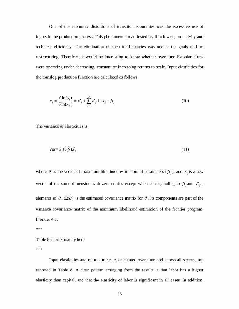
One of the economic distortions of transition economies was the excessive use of

inputs in the production process. This phenomenon manifested itself in lower productivity and

technical efficiency. The elimination of such inefficiencies was one of the goals of firm

restructuring. Therefore, it would be interesting to know whether over time Estonian firms

were operating under decreasing, constant or increasing returns to scale. Input elasticities for

the translog production function are calculated as follows:

jtjj

jhjji

ij x

xye βββ ++=

∂∂

= ∑=

ln)ln()ln( 2

1 (10)

The variance of elasticities is:

Var= ')( jj λθλ∧∧

Ω (11)

where θ is the vector of maximum likelihood estimators of parameters ( jβ ), and jλ is a row

vector of the same dimension with zero entries except when corresponding to jβ and jhβ ,

elements of θ . )(∧∧

Ω θ is the estimated covariance matrix for θ . Its components are part of the

variance covariance matrix of the maximum likelihood estimation of the frontier program,

Frontier 4.1.

***

Table 8 approximately here

***

Input elasticities and returns to scale, calculated over time and across all sectors, are

reported in Table 8. A clear pattern emerging from the results is that labor has a higher

elasticity than capital, and that the elasticity of labor is significant in all cases. In addition,

24

although capital has smaller elasticities, they are always significant except for the construction

sector in the balanced panel. Given such a pattern we focus on interpreting the results for the

panel estimations only. The results show that labor accounts for 72% of the value added (the

dependent variable) for both the unbalanced and the balanced panel, in the manufacturing

sector. It accounts for almost 66% for the agriculture sector and 91% for the construction

sector. While this pattern of input elasiticities would not be feasible under a market system, it

is not surprising in the context of a transition economy, characterized by outdated and labor-

intensive technology.

Returns to scale are calculated as the sum of individual elasticities from equation (10)

as follows:

∑∑ ∑∑∑== = ==

++==2

1

2

1

2

1

2

1

2

1ln

jjt

j jj

hjh

jjj xe βββυ (12)

In testing the deviation of actual returns to scale from constant returns to scale the test

statistic is the following:

)(1υ

υΩ−

=S where )(υΩ = ')( jj γθγ∧∧

Ω and ∑=

=2

1jjλγ (13)

This test statistic has a t-distribution. If the value of returns to scale is significantly larger than

unity then the firm operates in the increasing returns to scale region, while if it is significantly

less than unity then the firm operates in the decreasing returns to scale region.

The results of Table 8 show that the sum of elasticities is usually less than unity except

for year 1995 and the unbalanced panels for the agriculture and construction sector. The null

hypothesis of constant returns to scale is accepted in all cases. Hence, firms in Estonia, on

average, operate with the right input mix and are at the right point of their production function.

How then does this evidence reconcile with the efficiency improvements reported in Tables 6

and 7? One potential explanation is that efficiency gains have been achieved through the

decrease in the size of firms. As observed from Table 4, over time firms have reduced in size

25

as evidenced by the decline in the average employment, and have become more capital

intensive as evidenced by the increase in capital and the pattern of capital intensity ratio. This

data shows that Estonian firms, at the early transition, were characterized as more labor

intensive and over time substituted capital for labor, which may have contributed to higher

efficiency levels. However, Tables 6 and 7 reveal that firm size positively affects firm

efficiency. These findings are not necessarily contradictory as over time firms increase

efficiency by becoming more capital intensive with larger firms still being more efficient.

8. The Dynamics of Firm Technical Efficiency.

In this section we explore the dynamics of firm efficiency using the pattern of

efficiency scores calculated from the balanced panel. We opt for the use of the balanced panel

to avoid biases generated by the entry and exit of firms over time. The distributional pattern of

firm level efficiency, across firms of different ownership structures, as well as its evolution

over time, is a neglected issue in the literature. In investigating the distributional patterns of

firm efficiency, we are interested in distinguishing between firms that operate at low levels of

efficiency from those that operate at higher levels of efficiency. After all, firm level efficiency

is determined from different firm level characteristics, and, as such, we expect some firms to

be more efficient than others. Accordingly, we create five groups of firm level efficiency. The

first group includes all those firms that operate in between 0-20 % level of efficiency; the

second group includes firms that operate between 20-40 % level of efficiency and the other

three groups include firms that operate between 40-60%, 60-80% and 80-100% level of

efficiency, respectively. Graph 1, Graph 3 and Graph 5 represent the distribution of firms

according to this grouping over time for the manufacturing, agriculture and constructing

sector, respectively.

Graph 1, shows the distribution of firms belonging to the five efficiency groups for

manufacturing sector. From this graph we see that around 50% of firms in 1995 were

26

operating at the 0-20% and 20-40% levels of efficiency. This result is expected as early

transition was characterized by highly inefficient firms, who inherited from the centralized

market economy outdated capital, lack of advanced technology, expertise and resources

necessary to survive in the open market oriented economy. However, the percentage of firms

belonging to these levels of efficiency has decreased over time, while the percentage of firms

belonging to the last three efficiency groups (40-60%, 60-80% and 80-100%) has increased

over time. At this point, we can argue that reasons related to privatization, such as

restructuring and the introduction to market competition might have played an important role

to increasing firm efficiency. A slightly different pattern of increased firm efficiency over time

emerges from Graph 5, for the construction sector. The percentage of firms belonging to the

last efficiency group (80-100 %) has somewhat decreased over time, while the percentage of

firms belonging to the fourth efficiency group (60-80%) has increased over time with the other

groups experiencing marginal changes. In contrast, Graph 3 shows that efficiency distributions

for the agriculture sector have been quite stable over time, with the leas efficient group

shrinking in size. Overall, the conclusion to be drawn from these graphical illustrations is that

over time Estonian firms, on average, across all sectors have become more efficient as

expressed by the increasing percentage of them operating in high efficiency levels.

Further, we investigate the dynamics of efficiency across different ownership groups

and over time. Graph 2 shows that, firms in the manufacturing sector display increases in

efficiency over time. Among them, foreign firms are the most efficient over the whole period

and their efficiency persistently dominates that of the rest of ownership structures. Employee

owned firms follow up as the second best. This finding is consistent with the hypothesis that

employee ownership is expected to produce more interest alignment and more involvement of

employees and, in turn, better organizational performance compared to outsider and state

owned firms. This however, may also reflect the fact that employees have bought out the best

firms because of insider’s information. Also, this graph also shows that state owed firms

27

operate at the lowest level of technical efficiency until 1997. A relatively similar picture

emerges in the construction sector, displayed in Graph 6, where foreign owned firms display

the highest level of technical efficiency, followed by the domestic outsiders until mid 1997,

while employee owned firms display lower levels of technical efficiency, however, increasing

over time.

With respect to the agriculture sector, foreign firms entered the industry only in the last

two years (Graph 4). However, they are distinguished for their high level of technical

efficiency compared to the other ownership structures. The fact that foreign firms entered late

in the sector might suggest a protectionist policy of the government in order to increase its

competitiveness. Contrary to the manufacturing sector, the arguments against insider

ownership, especially employee ownership, find support here in that insider owned firms not

only display lower efficiency levels than outside private owned firms but also do not

experience increases in efficiency over time. In addition, the balanced panel for the agriculture

sector contains no state owned firms, except for in 1995, as they are privatized over time.

Overall, these results provide support to the theoretical predictions that privatization to

foreign ownership leads to higher firm efficiency. Furthermore, they provide partial support to

the theoretical arguments on the advantages/disadvantages of insider ownership. More

specifically, employee owned firms perform second best to foreign firms and display

increasing efficiency over time in the manufacturing sector. In contrast, employee owned

firms are ranked the last both in the construction and agriculture sector. In order to fully

explain the cross sector differences one needs to account for the pre-privatization performance

of firms. That is, it might be possible that given groups of owners had access to superior

information and, consequently, privatized better performing firms. We could speculate,

however, on these differences based on the sequence of privatization in these particular

sectors. The employee owned firms in the manufacturing sector are mostly those that went

through the leasing program at the beginning of transition and, consequently, were privatized

28

first. It is highly likely that these firms were better performing than those left for the

centralized privatization program. In contrast, employee owned firms in agriculture and

construction sectors are likely successors of collective farms. In their privatization priority

was given to private investors and usually those that did not attract any investors remained

under employee ownershipxii.

9. CONCLUSIONS

Using a representative panel of Estonian firms over the period 1993-1999 we

investigate the determinants of firm efficiency as well as its dynamics, applying the stochastic

frontier approach. The major benefit of using this method is that the parameters of both firm

level efficiency and production function are estimated simultaneously, resulting in efficient

estimates. Score efficiencies, obtained from the estimation of frontier, are then used to

investigate the dynamics of efficiency, which is a long neglected issue in the literature, as well

as firm’s returns to scale.

Our findings provide support to the hypothesis that a firm’s ownership structure is

important for the firm’s technical efficiency. For instance, we find that productive efficiency

increased over time across all ownership groups, with foreign owned firms being the most

efficient over time and across the three main economic sectors agriculture, manufacturing and

construction. In addition, employee owned firms have been the second best performing group

of firms for the manufacturing sector. This finding is consistent with the argument that

employee ownership is expected to produce more interest alignment and more involvement of

employees and, in turn, better organizational performance compared to outsider and state

owned firms (Dow, 2003). However, the fact that foreign and employee owned firms have the

highest levels of efficiency may also reflect the fact that they have bought out the best

performing firms at the beginning of the privatization Earle, Estrin and Leschenko (1996).

Nevertheless, the fact that efficiency for both groups increased over time suggests that this

29

argument might hold only for the beginning of privatization and that indeed both forms of

ownership have contributed significantly to firm efficiency, at least for the manufacturing

sector. In contrast, employee owned firms are ranked the last, both, in the construction and

agriculture sector. The efficiency distributions for these sectors support the arguments of

Blanchard and Aghion (1996) that privatization to outsider private owners leads to increased

firm efficiency as opposed to privatization to insiders. This conclusion, however, might not be

as strong if one takes into account the pre-privatization status of these firms. In fact, during

privatization, in these sectors priority was given to private investors and usually those firms

that did not attract any investors remained under insider ownership. Obviously the

restructuring of these firms needed significant investment in new capital and up to date

technology.

With respect to other firm characteristics, we find that firms that are foreign and

managerially owned, larger in size, with higher labor quality, and are privatized in the early

stages of transition, display higher levels of efficiency and as expected, soft budget constraints

are detrimental to firm efficiency. These results are consistent with the existing findings in the

literature.

Given that foreign ownership produces the highest levels of efficiency, the government

should strongly promote foreign direct investments, especially in form of joint ventures. This

way the government would promote economic growth. Furthermore, this policy should be

accompanied with hardening of soft budget constraints and promotion of training of

employees as important determinants of firm level efficiency.

We also find evidence of constant returns to scale across all economic sectors with

efficiency increasing over time. Estonian firms seem to increase efficiency by becoming more

capital intensive with larger firms still being more efficient.

30

REFERENCES

Aghion, Philippe, and Olivier J. Blanchard. 1998. “On Privatization Methods in Eastern Europe and their Implications,” Economics of Transition, 6(1), 87-98.

Aghion, Philipe and Wendi Carlin. 1996. “Restructuring Outcomes and the Evolution of Ownership Patterns in Central and Eastern Europe,” Economics of Transition, 4(2), 372-388. Aigner, Dennis, Lovell, C.A. Knox, and Schmidt, Peter. 1977. “Formulation and Estimation of Stochastic Frontier Production Function Models,” Journal of Econometrics, 6(1), 21-37. Anderson, James H., Georges Korsun, and Peter Murrell. 2000. “Which Enterprises (Believe They) have Soft Budgets after Mass Privatization? Evidence from Mongolia,” Journal of Comparative Economics, 28(2), 19-246. Angrist, Joshua D. and Alan B. Krueger. 2001. “Instrumental Variables and the Search for Identification: From Supply and Demand to Natural Experiments.” Journal of Economic Perspectives, 15(4), 69-85. Aw Bee-Yan, Sukkyn Chung and Mark J. Roberts. 2000. “Productivity and Turnover in the Export Market: Micro-level Evidence from the Republic of Korea and Taiwan,” The World Bank Economic Review, 14(1), 65-90. Battese, G.E. and Corra, G.S. 1977. “Estimation of a Production Frontier Model: With Application to the Pastoral Zone of Eastern Australia”, Australian Journal of Agricultural Economics, 21, 169-179. Bernard, Andrew B. and J. Bradford Jensen. 1999. “Exceptional Exporter Performance: Cause, Effect, or Both?,” Journal of International Economics, Vol. 47(1), 1-25. Bevan, Alan, A., Saul Estrin, and Mark Schaffer. 1999. “Determinants of Enterprise Performance during Transition,” CERT Working Paper No. 99/03, Heriot-Watt Univesrity. Blanchard, Olivier, Rudiger Dornbuch, Paul Krugman, Richard Layard and Lawrence Summers. 1991. Reforms in Eastern Europe. Cambridge Massachusetts, MIT Press. Blanchard, O. and R. Layard. 1992. “How to Privatize,” H. Siebert (ed.), The Transformation of Socialist Economies, Tübingen: Mohr, pp. 27-47. Blanchard, Olivier, J., and Philippe Aghion. 1996. “On Insider Privatization,” European Economic Review, Vol.40, 759-766. Boycko, Maxim, Andrei Shleifer and Robert W. Vishny. 1996. “A Theory of Privatization,” The Economic Journal, Vol. 102, 309-319. Boycko, Maxim, Andrei Shleifer and Rober W. Vishny. 1993. “Privatizing Russia,” Brooking Papers on Economic Activity, 2, 139-192.

31

Brada, J.C., A.E. King, and C.Y. Ma. 1997. “Industrial economics of the transition: determinants of enterprise efficiency in Czechoslovakia and Hungary,” Oxford Economic Papers, 49, 104-127. Brown, David J. and S. John Earle. 1999. “Does Market Structure Matter? New Evidence from Russia,” CEPR Discussion Paper, London, England. Brown, David, J. and John S. Earle. 2001. “Privatization, Competition, and Reform Strategies: Theory and Evidence from Russian Enterprise Panel Data”, SITE, Stockholm School of Economics. Brown, David and John Earle. 2001. “Competition Enhancing Policies and Infrastructure: Evidence from Russia,” CEPR Discussion Paper 3022, London, England. Carlin, Wendy and Michael Landesman. 1997. “From Theory into Practice? Restructuring and Dynamism in Transition Economies,” Oxford Review of Economic Policy, 13: 77-105. Carlin, Wendy, Steven, Fries, Mark Schaffer, and Paul Seabright. 2001. “Competition and Enterprise Performance in Transition Economies: Evidence from a Cross-Country Survey,” Working Paper, Department of Economics, University College, London. Claessens, Stijn, and Kyle Peters. 1997. “State Enterprise Performance and Soft Budget Constraints: The case of Bulgaria,” Economics of Transition, 5, 2:305-322. Clerides, K. Sofronis, Saul Lach and James R. Tybout. 1998. “Is Learning by Exporting Important? Micro-Dynamic Evidence from Colombia, Mexico, and Morocco,” Quarterly Journal of Economics, Aug: 903-947. Coelli, Tim. 1996. “A Guide to Frontier Version 4.1: A Computer Program fro Stochastic Frontier Production function and Cost Function Estimation,” CEPA Working Paper No. 96/07, University of New England, Armidale, Australia. Coelli, Tim, G.E. Battese, and D.S.P. Rao. 1998.“An Introduction to efficiency and productivity analysis,” Kluwer Academic Publishers, Boston. Coricelli, Fabrizio and Djankov, Simeon. 2001. “Hardened Budgets and Enterprise Restructuring: Theory and Application to Romania,” Journal of Comparative Economics, 29 (4), 749-763. Danilin, V.I., Ivan S. Materov, Steven Rosefielde, and C.A. Knox Lovell. 1985. “Measuring Enterprise Efficiency in the Soviet Union: A Stochastic Frontier Analysis,” Economica, 52, 225-233. Djankov, Simeon and Peter Murrell. 2002. “Enterprise Restructuring in Transition: A Quantitative Survey,” Journal of Economic Literature, Vol. 40(3), 739-792. De Mello, L. R. Jr. 1997. “Foreign Direct Investment in Developing Countries and Growth: A Selective Survey,” The Journal of Development Studies, Volume 34(1): 1-34. Dow, Gregory K. 2003. Governing the Firm: Workers Control in Theory and Practice. Cambridge University Press.

32

D’Souza J. and W. Meggionson. 1999. “The Financial and Operating Performance of Privatized Firms During the 1990s,” Journal of Finance, Vol. 54 (4), 1397-1438. Earle, John and Saul Estrin. 1996. “Employee Ownership in Transition,” in Frydman, C.W. Gray, A. Rapaczynski (eds.), Corporate Governance in Central Europe and Russia, Budapest: CEU Press. Earle, John, Saul Estrin and Larisa, L., Leschenko. 1996. “Ownership Structures, Patterns of Control, and Enterprise Behavior in Russia”, in Commander, Simon, Fan, Qimiao, and Schaffer, Mark E. (eds.), Enterprise Restructuring and Economic Policy in Russia, EDI Development Studies, Washington, D.C.: World Bank. Earle, John S., and Saul Estrin. 1997. “After Voucher Privatization: The Structure of Corporate Ownership in Russian Manufacturing Industry”, CEPR Discussion Paper No. 1736. Estrin, Saul and Mike Wright. 1999. “Corporate Governance in the Former Soviet Union: An Overview”, Journal of Comparative Economics, Vol. 27(3), 398-421. European Bank for Reconstruction and Development. Transition Report. 1999. European Bank for Reconstruction and Development. Transition Report. 2000. Filatochev, Igor, Irina Grosfeld, Judit Karsai, Mike Wright and Trevor Buck. 1996. “Buy-outs in Hungary, Poland and Russia: Governance and Finance Issues”, Economics of Transition, Vol. 4(1), 67-88. Filer, Randall and Jan Hanousek. 2001. “Informational Content of Price Sets Using Excess Demand: The Natural Experiment of Czech Voucher Privatization”, European Economic Review, Vol. 45(9), 1619-1649. Forsund, Finn R., Lovell, C. A. Knox, Schmidt, Peter. 1980. “A Survey of Frontier Production Functions and of Their Relationship to Efficiency Measurement”, Journal of Econometrics, Vol. 113(1), 5-25. Frydman, R., Cheryl Gray, Marek Hessel, and Andrzej Rapaczynski. 1999. “When Does Privatizatio Work? The Impact of Private Ownership on Corporate Performance in The transition Economies”, The Quarterly Journal of Economics, November, 1153-1191. Frydman, R., E. S. Phelps, A. Rapaczynski and A. Shleifer. 1993. “Needed Mechanisms of Corporate Governance and Finance in Eastern Europe”, Economics of Transition, Vol. 1(2), 171-207. Frydman, R. and A. Rapaczynski. 1991. “Privatization and Corporate Governance in Eastern Europe: Can a Market economy be Designed.” CVSTARR Working Paper Series, No. 91-52. Funke, Michael and Jörg Rahn. 2002. “How efficient is the East German Economy? An exploration with microdata,” Economics of Transititon, 10(1), 201-223. Greene, William H. 2003. Econometric Analysis. Pearson Education, Inc., Upper Saddle River, New Jersy.

33

Jondrow, J., C.A.K. Lovell, I.S. Materov and P. Schmidt. 1982. “On Estimation of Technical Inefficiency in the Stochastic Frontier Production Function Model,” Journal of Econometrics, 19, 233-238. Jones, Derek C., Mark Klinedinst and Charles Rock. 1998. “Productive Efficiency during Transition: Evidence from Bulgarian Panel Data,” Journal of Comparative Economics, 26, p. 446-464. Jones, Derek C., and Niels Mygind. 2002. “Ownership and Productive Efficiency: Evidence from Estonia,” Review of Development Economics, 6(2), 284-301. Kalmi, Panu. (2002). On the (In)stability of Employee Ownership: Estonian Evidence and Lessons for Transition Economies. Ph.D. Dissertation. Copenhagen Business School, Ph.D. Serie 10. Kodde, David A., and Franz C. Palm. 1896. “Wald Criteria for Jointly Testing Equality and Inequality Restrictions” Econometrica, 54(5), 1243-1248. Konings, Jozef and Alexander Repkin. 1998. “How Efficient are Firms in Transition Countries? Firm level evidence from Bulgaria and Romania,” CEPR Discussion Paper No. 1839. Kong, Xiang, Robert E. Marks, and Guang Hua Wan. 1999. “Technical Efficiency, Technological Change and Total Factor Productivity Growth in Chinese State-Owned Enterprises in the Early 1990s,” Asian Economic Journal, 13(3), 267-281. Kornai, Janos. 1980. “ ‘Hard’ and ‘Soft’ Budget Constraints,” Acta Oeconomica, 25,3-4: 231-245. La Porta, Rafael and Florencio Lopez-de-Silanes. 1997. “The Benefits of Privatization: Evidence From Mexico”, NBER Working Paper No. 6215. Lipton, David and Jeffrey Sachs. 1990. “Privatization in Eastern Europe: The Case of Poland.” Brooking Papers on Economic Activity, Volume 2: 293-342. Megginson, William and Jeffry M. Netter. 2001. “From State to Market: A Survey of Empirical Studies on Privatization”, Journal of Economic Literature, Vol. 39, 321-389. Meeusen W, van den Broeck J. 1977. “Efficiency Estimation from Cobb-Douglas Production Functions with Composed Error,” International Economic Review, 18: 435-444. Mygind, Niels. 2000. “Privatization, Governance and Restructuring of Enterprises in the Baltics.” OECD Working Paper Series, No. 6. Piesse, Jenifer, and Colin Thirtle. 2000. “A Stochastic Frontier Approach to Firm Level Efficiency, Technological Change and Productivity during Early Transition in Hungary,” Journal of Comparative Economics, 28, 473-501. Prasnikar, Janez, Jan Svejnar and Mark Klinedinst. 1992. “Structural Adjustment Policies and Productive Efficiency of Socialist Enterprises,” European Economic Review, 36, 179-199.

34

Roberts, Mark and James Tybout. 1997. “An Empirical Model of Sunk Costs and the Decision to Export.” American Economic Review, Vol. 87(4), pp. 545-64. Schaffer, Mark E. 1998. “Do Firms in Transition Economies Have Soft Budget Constraints? A Reconsideration of Concepts and Evidence”, Journal of Comparative Economics, Vol.26, 80-103. Smith, Kerry, Beom-Cheol Cin, and Milan Vodopivec. 1997. “Privatization Incidence, Ownership Forms and Firm Performance: Evidence from Slovenia”, Journal of Comparative Economics, 25 (2), 158-179. Smith, Peter. 1997. “Model Misspecification in Data Envelopment Analysis,” Annals of Operations Research, 73, 233-252. Tong, Christopher. 1999. “Production Efficiency and its spatial disparity across China’s TVEs. A Stochastic Production Frontier Approach,” Journal of Asian Economics, 10, 415-430.

35

APPENDIX Table 1: Variable Definition

Variables Definition Value Added The dependant variable is constructed as the sum of Net Profit,

Depreciation and Labor Cost (Wage Salary +Social Security +interest costs). Expressed in thousands of kroons.

Employment Firm's average number of employees per year. Capital Capital is calculated as the average of fixed assets at the beginning and

end of year. Expressed in thousands of kroons. Herfindahl (3 digit) Used to capture monopoly power

Herfindahlj =∑ ⎟⎟⎠

⎞⎜⎜⎝

⎛i

j

i

SaleSale

2

j-industry, i -firm

Constructed at the three digit industry classification. Dominant Ownership Dummy This is a dummy equal to 1 if the share in equity owned by a group for

that year is greater than that owned by any other group. Firm’ Debt (used to construct SBC dummy)

Is constructed as the sum of Current Debt and Current Payables. Expressed in thousands of kroons.

Net Financing (used to construct SBC dummy)

Constructed as [Debt(t)- Debt(t-1)-Interest Cost(t)]/Fixed Assets

EBITD (used to construct SBC dummy)

Earnings before Interests, Profit Taxes and Depreciation are equal to the sum of Gross Profit and Depreciation. Expressed in thousands of kroons.

Dummy Soft Budget Constraint Equals 1 if Net financing>0 & EBITD<0, zero otherwise.

Average Labor Cost Used to proxy labor quality. Expressed in thousands of kroons. Age of Privatization Shows the number of years a firm has been operating as private. Sales Net sales are expressed in thousands of kroons. Available at firm level. Investment/Sales The share of expenditure on new machinery and equipment to net sales

of the firm. Used to account for investment in new technology. Export/Sales The share of firm’s export to net sales. Dummy High Tech Industriesxiii This is a dummy equal to 1 if the firm belongs to a high tech industry.

Such industries are: 1) Manufacture of chemicals and chemical products. 2) Manufacture of electrical and optical equipment4

Firm Size The logarithm of firm level employment. dt Time Trend: 1) Included at the production function to account for

technical changes in productivity. 2) Also included at the inefficiency function to account for temporal changes in technical inefficiency.

dj Industry dummy, constructed on a two-digit level industry classification Note: All data, except average number of employees and ownership shares, has been deflated to 1993 prices before variable construction.

36

Table 2: The Distribution of Firms by Year and Economic Sectors

Year Agriculture Manufacture Construction Total 93 55 218 44 317 94 47 216 48 311 95 45 264 61 370 96 35 256 60 351 97 37 229 53 319 98 34 197 44 275 99 28 170 33 231

Total 281 1,550 343 2174 Table 3: The Dynamics of the Dominant Ownership Structure.

Year Domestic Outsider

Employees Foreign Managers State Total

93 64 40 28 27 158 317 94 74 45 33 35 124 311 95 80 40 34 39 177 370 96 98 37 45 49 122 351 97 85 23 45 55 111 319 98 76 21 42 47 89 275 99 93 30 54 53 1 231

Total 570 236 281 305 782 2174 Table 4: Mean and Standard Deviations of Main Variables over Time. Year

Value Added

Capital Labor Capital/ Labor

VaAdded/Labor

Herfindahl

Avg. Labour Cost

1Export/Y Invest./Y

93 4758.63 (11128)

5513.48 (13669.16)

182.11 (380.09)

33.79 (86.63)

24.78 (33.84)

0.27 (0.16)

3019.46 (5698.6)

.

0.400 (2.79)

94 4306.66 (10151.71)

5747.13 (14757.23)

152.33 (275.62)

50.58 (217.31)

29.12 (45.9)

0.28 (0.18)

3333.58 (6422.13)

0.24 (0.30)

0.26 (1.87)

95 3722.41 (8965.83)

5480.89 (13123.93)

152.30 (260.88)

45.81 (193.4)

23.41 (32.0)

0.24 (0.17)

2770.80 (5214.29)

0.25 (0.31)

0.17 (0.91)

96 5087.05 (10481.34)

6077.55 (15186.6)

152.72 (284.24)

46.74 (195.36)

32.28 (30.28)

0.25 (0.17)

4014.55 (7755.55)

0.26 (0.32)

0.099 (0.28)

97 6216.15 (11537.03)

6534.45 (14987.78)

145.73 (255.19)

51.47 (159.25)

55.16 (298.65)

0.26 (0.19)

4344.16 (7708.72)

0.28 (0.32)

0.094 (0.19)

98 6559.6 (10847.16)

8235.95 (16677.36)

151.53 (255.83)

54.58 (97.17)

43.58 (38.05)

0.22 (0.18)

4895.68 (8033.01)

0.27 (0.32)

0.19 (1.42)

99 6991.69 (11925.39)

9887.60 (21169)

130.96 (174.37)

65.01 (100.59)

38.69 (163.31)

0.24 (0.19)

4779.39 (6832.42)

0.29 (0.33)

0.07 (0.12)

Total 5249.60 6591.39 153.39 48.87 34.69 0.25 3801.45 0.26 0.18

Note: 1 Export data for year 1993 is missing.

2 This is the total number of observations over time excluding missing values of respective variables.

37

Table 5A: Hypotheses Tests Results for Manufacturing Manufacturing

Test 1: H0: Cobb-Douglas is the appropriate functional form versus Translog.

Test Statistic (2

95.0,3χ ) = 7.81 (Panel 2

95.0,6χ =12.59)

1995 1996 1997 1998 1999

Unbalanced Panel

Balanced Panel

Test Statistic (Likelihood Ratio)

4.42 9.96 60.16 12.56 16.42 76.14 37.48

Result Accept Reject Reject Reject Reject Reject Reject

1Test 2: H0: γ = 0α = kα =0 Cross-Section: (2

95.0,24χ ) = 35.827 Panel: (2

95.0,25χ ) =37.066

γ value 0.89 0.84 0.92 0.84 0.85 0.89 0.82

Test statistic (Likelihood Ratio)

113.32 151.47 172.97 162.66 95.31 557.1 429.07

Result Reject Reject Reject Reject Reject Reject Reject Decision Front Front Front Front Front Front Front

Test 3: H0: 0=kα Cross Section 295.0,22χ =33.92 Panel:

295.0,23χ = 35.17

Test Statistic (LR)

76.44 101.46 101.92 109.2 71.02 315.74 255.12

Result Reject Reject Reject Reject Reject Reject Reject

Test 4: H0: 0=== jtttt βββ 2

95.0,4χ =9.49

Test Statistic (LR)

- - - - - 9.82 9.54

Result - - - - - Reject Reject

1The test statistics has a mixed Chi2 distribution, critical values taken from Kodde and Palm (1986).

38

Table 5B: Hypotheses Tests Results for Agriculture and Construction Agriculture Construction

Test 1: H0: Cobb-Douglas is the appropriate functional form vs. Translog. 2

95.0,6χ =12.59

Unbalanced Panel

Balanced Panel Unbalanced Panel Balanced Panel

Test Statistic (Likelihood Ratio)

16.42 36.22 12.94 14.14

Result Reject Reject Reject Reject 1Test 2: H0: H0: γ = 0α = kα =0

295.0,14χ =23.069

γ value 0.79 0.56 0.87 0.75 Test stat (Likelihood Ratio)

88.05 85.16 83.37 39.99

Result Reject Reject Reject Reject Decision Frontier Frontier Frontier Frontier

Test 3: H0: 0=kα 2

95.0,12χ = 21.03

Test stat (Likelihood Ratio)

61.24 83.86 40.8 20.86

Decision Reject Reject Reject Reject

Test 4: H0: 0=== jtttt βββ 2

95.0,4χ =9.49

Test stat (Likelihood Ratio)

17.84 30.84 10.48 11.92

Decision Reject Reject Reject Reject 1The test statistics has a mixed Chi2 distribution, critical values taken from Kodde and Palm (1986).

39

Table 6: Cross-Section Frontier Estimation of the Translog Production Function. Manufacturing Sector. Production

1995

1996

1997

1998

1999

Fixed Effects UnBalanced

Fixed EffectsBalanced

5.34*** 4.48*** 3.92*** 3.88*** 3.41*** 0.26*** 0.21*** Constant (3.48) (5.48) (6.00) (5.75) (3.96) (23.84) (13.35) 0.010 -0.173 0.155 -0.040 0.111 0.146 0.45*** LnK (0.06) (-0.99) (0.80) (-0.26) (0.59) (1.02) (2.81) 0.94** 1.07*** 0.69** 1.09*** 1.135*** 0.027 0.39* LnL (2.20) (4.00) (2.33) (4.20) (3.73) (0.10) (1.41)

-0.026* 0.039*** 0.082*** 0.031*** 0.029*** 0.002 0.015** LnK2 (-1.82) (2.90) (5.1) (2.98) (2.34) (0.25) (1.97) -0.044 0.015 0.219*** -0.011 0.020 0.149*** 0.165*** LnL2 (-0.80) (0.41) (5.69) (-0.26) (0.42) (3.77) (4.11) 0.076* -0.059* -0.257*** -0.046* -0.078** -0.063** -0.142*** LnK*LnL (1.61) (-1.59) (-7.31) (-1.61) (-2.18) (-1.84) (-4.22)

Time Trend (T) - - - - - 0.129** 0.11* (1.71) (1.37) T* LnK - - - - - 0.054*** 0.039*** (6.24) (4.63) T* LnL - - - - - -0.052*** -0.022* (-3.58) (-1.45) Time Trend Squared - - - - - -0.035*** -0.038*** (-4.02) (-4.31) Inefficiency Function

3.49*** 2.63*** 1.36* 1.41* 1.83** -5.44*** -3.79*** Constant (2.68) (2.92) (1.35) (1.43) (2.05) (-5.14) (-3.96) 0.137 -0.87* 0.33 -0.046** 0.066 -1.63** -2.72*** Dummy Foreignt-1 (0.48) (-1.34) (0.61) (-2.08) (0.12) (-2.24) (-2.80) -0.006 -0.194* -0.403 -0.054 0.057 2.74*** 1.57*** Dummy Managert-1 (-0.02) (-1.39) (-0.84) (-0.11) (0.10) (3.48) (1.75) 0.24 -0.199 0.084 0.560 0.428 2.85*** 3.41*** DummyDomestict-1

(1.11) (-0.48) (0.19) (1.17) (0.80) (4.29) (3.58) 0.31 0.407 -0.26 0.259 0.112 2.67*** 2.84*** Dummy Statet-1

(1.08) (0.66) (-0.45) (0.46) (0.19) (3.51) (3.31) 0.039 -0.170 -0.089 -0.182 -0.170 -0.796* -2.174*** Firm Sizet-1 (0.19) (-1.21) (-0.66) (-1.22) (-1.21) (-1.58) (-2.72)

-0.059*** -0.13*** -0.079*** -0.064*** -0.039*** -0.015** -0.093*** Avg. Labor Costt-1 (-8.92) (-8.33) (-4.41) (-3.55) (-3.52) (-1.83) (-4.36)

-0.082*** 0.069 0.881*** 1.459** 0.091 -0.136** -0.104* Invest/Sales t-1 (-3.33) (0.91) (3.33) (2.08) (0.55) (-2.06) (-1.39) -0.008 0.017 0.048 0.014 0.069 -2.902*** 1.69 Export/Sales t-1 (-0.04) (0.04) (0.14) (0.04) (0.25) (-3.09) (1.21)

0.84*** 0.732 0.904*** 1.128*** 0.425* 3.86*** 1.789*** Dummy SBC t-1 (4.45) (0.80) (3.26) (3.33) (1.53) (5.77) (2.88) -0.137 1.102 -0.306 0.412 0.221 -0.980 -1.58* Herfindahl (3digit) (-0.19) (1.22) (-0.43) (0.50) (0.30) (-1.00) (-1.47) 0.013 0.171* -0.011 0.017 -0.021 0.162 -0.044 Age of Privatization (0.22) (1.33) (-0.14) (0.29) (-0.40) (0.88) (-0.21)

Time Trend - - - - -0.018 0.102 (-0.12) (0.55) Dummy High Tech -0.211 -0.698 1.028* 0.375 0.365 - - (-0.33) (-0.98) (1.35) (0.53) (0.56) Industry Dummy yes yes yes yes yes - - Mean Efficiency 0.14 0.525 0.503 0.60 0.523 0.58 0.63 ME of Technical change1) - - - - - 0.12 0.098 No. Obs. 169 243 223 192 163 990 740

Note: ***, ** and * significant at 1%, 5% and 10% respectively. The marginal effect of technical change can be estimated by taking the derivative of equation (9) with respect to time and evaluate it at the geometric mean of respective variables.

40

Table 7: Fixed Effects Panel Data Frontier Estimation of the Translog Production Function. Agriculture and Construction Sector.

Fixed Effects Agriculture Sector Fixed Effects Construction Sector Production Unbalanced Panel Balanced Panel Unbalanced Panel Balanced Panel

0.146*** 0.318*** 0.218*** 0.21*** Constant (5.78) (4.90) (5.21) (2.58) -0.115 -0.597** 0.109 0.372 LnK (-0.49) (-2.32) (0.46) (0.55) 1.129* -0.922 1.9*** 1.27* LnL (1.39) (-0.87) (4.07) (1.45) 0.027 0.003 0.022 0.06* LnK2 (0.98) (0.06) (1.15) (1.52) -0.076 0.087 -0.048 0.080 LnL2 (-0.62) (0.50) (-0.57) (0.49) -0.003 0.168 -0.069 -0.21* LnK*LnL (-0.02) (1.04) (-0.93) (-1.46)

0.492*** 0.342** 0.367*** -0.093 Time Trend (T) (3.48) (2.19) (2.37) (-0.34) -0.018 0.065** 0.018 -0.039 T*LnK

(-0.60) (1.90) (0.82) (-1.01) 0.001 -0.079* -0.055* 0.087 T*LnL (0.03) (-1.51) (-1.41) (0.99)

-0.052*** -0.06*** -0.034** 0.002 Time Trend squared (T2) (-3.21) (-3.04) (-2.22) (0.09)

-2.456*** -0.069 -1.55* -1.45* Constant

(-4.20) (-0.20) (-1.62) (-1.57) -2.373** -0.270 1.078 0.309 Dummy Foreignt-1 (-2.25) (-0.34) (1.11) (0.33)

-2.070** -0.503 -0.720 -0.540 Dummy Managert-1 (-2.18) (-1.06) (-1.21) (-0.79)

1.116** 0.348* -2.657** -2.035* DummyDomestict-1

(2.30) (1.32) (-2.12) (-1.33) 0.003 -0.510 -2.84*** -2.67** Dummy Statet-1

(0.009) (-0.92) (-2.46) (-2.02) -0.134 0.284 -1.14*** -0.97*** Firm Sizet-1 (-0.15) (0.41) (-2.37) (-2.36) -0.006 0.014 0.024** 0.010 Avg. Labor Costt-1 (-0.27) (0.75) (1.86) (0.61)

-4.723*** 0.169 -1.93** -2.068** Invest/Sales t-1

(-3.15) (0.17) (-2.00) (-2.28) 0.959 0.846 5.73** 5.002** Export/Sales t-1 (0.69) (0.80) (2.18) (2.22) 1.33** -0.532 0.244 -0.231 Dummy SBC t-1 (2.10) (-0.97) (0.51) (-0.36) -0.580 1.348 0.336 -1.128 Herfindahl (3digit) (-0.55) (0.83) (0.34) (-0.94)

-0.713*** 0.092 0.017 -0.504* Age of Privatization (-2.47) (0.13) (0.09) (-1.44)

1.472*** 0.092 0.4* 0.88** Time Trend (4.23) (0.13) (1.46) (1.91)

Mean Efficiency 0.75 0.62 0.70 0.74 ME of Technical change1) 0.477 0.337 0.349 -0.0914 No. Obs. 156 100 219 120 Note: ***, ** and * significant at 1%, 5% and 10% respectively. 1) The marginal effect of technical change can be estimated by taking the derivative of equation (9) with respect to time and evaluate it at the geometric mean of respective variables.

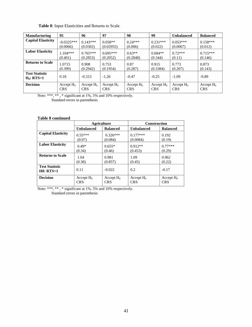
41

Table 8: Input Elasticities and Returns to Scale.

Manufacturing 95 96 97 98 99 Unbalanced Balanced Capital Elasticity -0.0325***

(0.0066) 0.143*** (0.0302)

0.058** (0.02955)

0.24*** (0.006)

0.231*** (0.022)

0.053*** (0.0067)

0.158*** (0.012)

Labor Elasticity 1.104*** (0.401)

0.765*** (0.2853)

0.695*** (0.2052)

0.63** (0.2848)

0.684** (0.344)

0.72*** (0.11)

0.715*** (0.146)

Returns to Scale 1.0715 (0.399)

0.908 (0.2942)

0.753 (0.1954)

0.87 (0.287)

0.915 (0.3384)

0.773 (0.207)

0.873 (0.143)

Test Statistic H0: RTS=1 0.18 -0.313 -1.26 -0.47 -0.25 -1.09 -0.89

Decision Accept H0 CRS

Accept H0 CRS

Accept H0 CRS

Accept H0 CRS

Accept H0 CRS

Accept H0 CRS

Accept H0 CRS

Note: ***, ** , * significant at 1%, 5% and 10% respectively. Standard errors in parenthesis

Table 8 continued

Agriculture Construction Unbalanced Balanced Unbalanced Balanced Capital Elasticity 0.55***

(0.07) 0.326*** (0.084)

0.177*** (0.0084)

0.192 (0.19)

Labor Elasticity 0.49* (0.34)

0.655* (0.46)

0.912** (0.453)

0.77*** (0.29)

Returns to Scale 1.04 (0.38)

0.981 (0.857)

1.09 (0.45)

0.962 (0.22)

Test Statistic H0: RTS=1 0.11 -0.022 0.2 -0.17

Decision Accept H0 CRS

Accept H0 CRS

Accept H0 CRS

Accept H0 CRS

Note: ***, ** , * significant at 1%, 5% and 10% respectively. Standard errors in parenthesis

42

Graph 1

05

101520253035

Perc

enta

ge o

f Fi

rms

95 96 97 98 99

Year

Percentage of Firms by Efficiency Groups: Balanced Panel of the Manufacture Sector

0-2020-4040-6060-8080-100

Graph 2

The Dynamics of Firm Efficiency by Ownership Group for the Balanced Panel of the Manufacture Sector

0.3

0.45

0.6

0.75

0.9

95 96 97 98 99

Years

Tech

nica

l Effi

cien

cy

Dom

Empl

For

Man

Stat

43

Graph 3

0.005.00

10.0015.0020.0025.0030.0035.0040.00

Perc

enta

ge o

f Fi

rms

95 96 97 98 99

Year

Percentage of Firms by Efficiency Groups: Balanced Panel of the Agriculture Sector

0-2020-4040-6060-8080-100

Graph 4

The Dynamics of Firm Efficiency by Ownership Groups for the Balanced Panel of the Agriculture Sector

0

0.2

0.4

0.6

0.8

1

1.2

95 96 97 98 99

Years

Tech

nica

l Effi

cien

cy

Dom

Empl

For

Man

Stat

44

Graph 5

0.0010.0020.0030.0040.0050.0060.0070.00

Perc

enta

ge o

f Fi

rms

95 96 97 98 99

Year

Percentage of Firms by Efficiency Groups: Balanced Panel of the Construction Sector

0-2020-4040-6060-8080-100

Graph 6

The Dynamics of Efficiency by Ownership Groups for the Balanced Panel of the Construction Sector

0.4

0.5

0.6

0.7

0.8

0.9

1

95 96 97 98 99

Years

Tech

nica

l Effi

cien

cy

Dom

Empl

For

Man

Stat

45

i In their study of Russia, Earle, Estrin and Leschenko (1996) point out many cases of insider buyouts at very favorable prices even before the official state privatization program. ii However, it has been observed that soft budget constraints distort the effect of competitive pressure on firm performance (Schafer, 1998; Coricelli and Djankov, 2001). iiiWe check for inconsistencies using different criteria. For instance, a firm’s capital at the beginning and end of each year should be positive; sales should be positive; labor cost in a given year should be positive; average employment per year should be positive and equal or greater than 10; investment in new machines and equipment should be non-negative; and the ownership shares should add up to 100. This leads to a drop of about 10% of observations, resulting in 3578 observations. Furthermore, one of the main weaknesses of the stochastic frontier approach is the presence of outliers, which push the frontier up for all the firms in the sample, causing pronounced firm inefficiency. Therefore, before carrying out the analysis, we perform a series of checks for outliers in the following variables: capital stock, employment, wages and salaries, sales and value added. These consistency checks reveal that eighteen observations belonging to 6 firms are outliers. For these observations employment, capital or sales are more than four times that of the sample average. Consequently, they are dropped from the initial sample. Finally, since we estimate the frontier for three main economic sectors, namely, agriculture, manufacturing and construction, the final number of observations in the analysis is 2174. iv Our measure of soft budget constraint suffers from two further pitfalls. First, it might fail to capture firms with genuine soft budget constraints. More specifically, a firm with negative earnings and zero net financing in a given period is still experiencing soft budget constraint if it expects to receive financing in the future. This measure of soft budget constraint, however, involves unobservables and it will always fail to capture the true degree of soft budget constraint. Second, our measure of soft budget constraint might mistakenly classify as firms that experience soft budget constraints those firms that in fact do not. For example, it could well be the case that young or newly established firms might be loss-making during the first years of their existence until they gain market share and establish relations with financial institutions. In the meantime, they might be receiving outside financing in response to their long-term growth potential. Again, this involves unobservables and as such it is not possible to account for using accounting data. Both these problems generate biases in the real number of firms that experience soft budget constraints, and as such, should be kept in mind in the interpretation of results. v Another technique that estimates firm efficiency is the data envelopment analysis (DEA). This is a non-parametric programming technique. The advantage of DEA is that one need not specify any distributional form for the inefficiency term and for the functional form of the production function. The disadvantage is that it does not account for noise and hence any departure from the frontier is inefficiency. Therefore, this model produces inefficiency scores that are particularly large compared to other frontier models. This assumption is difficult to sustain at the firm level in the presence of measurement error, missing variables and uncontrollable environment factors that can affect production such as the weather. In this paper we pursue the stochastic frontier approach for several reasons. First, this estimation strategy is more likely to be appropriate for transition and developing economies, where the data is heavily influenced by measurement error in the sectors we investigate (agriculture, manufacturing and construction) where the data is also heavily influenced by variables such as weather and disease. Second, we use a data set that is large enough to justifiy the use of parametric estimations. Third, we are also interested in knowing what firm and industry characteristics affect firm level efficiency and the stochastic frontier allows us to do this in a simultaneous estimation. Finally, it allows us to perform tests of hypotheses concerning the existence of inefficiencies, the structure of the production technology and economies of scale. vi A firm’s total inefficiency is composed of allocative and technical inefficiency. Estimating total inefficiency would require data on output and input prices. Unfortunately the data we used in the analysis does not provide information on output and input prices. Therefore, we are able to estimate technical inefficiency only. vii A similar approach is followed by Piesse and Thirtle (2000). viii A problem is that uit is unobservable, hence its prediction is needed. The best predictor for uit is the conditional expectation of uit given the value of eit=vit -uit (Jondrow, Lovell, Materov and Schmidt, 1982). ix The likelihood ratio test statistic is ))}(log())({log(2 10 HlikelihoodHlikelihood −−=λ . It has a

2kχ distribution where k is the number of parameters assumed to be zero in the null hypothesis. Log

likelihoods needed to construct the test statistics are estimated from the Frontier 4.1 program as part of the frontier output (see Coelli, Battese and Rao, 1998). x The literature uses interchangeably two terms, endogeneity and selection bias. Nevertheless, they are both used in the same context i.e., the best firms were given out for privatization and that informed and/or powerful groups of potential owners privatized these firms. xi A different strategy followed in a previous version of the paper was to instrument the current ownership structure with its predicted values obtained from a probit estimation. Firm level characteristics such as firm size, its capital intensity, labor productivity, labor quality and a lag of firms’ ownership structure were used to predict firms’ current ownership structure. The results obtained, showed that the dynamics of efficiency, for instance, for

46

the manufacturing sector, was almost identical to the one reported in this paper (graph 2). The dangers of this approach, however, as Angrist and Krueger (2001) have pointed out, are that unless the first stage nonlinear equation happens to be exactly specified, the use of its predicted values in the second stage will lead to misspecification bias. This graph is available upon request. xii Further evidence on these issues is provided in Kalmi (2002). xiii According to the Estonian Technology Agency 2002 these industries have the highest innovation expenditure intensity.