Physical Topology Logical Topology Authentication Licensing.
Upload
phungkhanhCategory
view
224download
0
This paper is included in the Proceedings of the 2017 USENIX Annual Technical Conference (USENIX ATC ’17).
July 12–14, 2017 • Santa Clara, CA, USA
ISBN 978-1-931971-38-6
Open access to the Proceedings of the 2017 USENIX Annual Technical Conference
is sponsored by USENIX.
deTector: a Topology-aware Monitoring System for Data Center Networks
Yanghua Peng, The University of Hong Kong; Ji Yang, Xi’an Jiaotong University; Chuan Wu, The University of Hong Kong; Chuanxiong Guo, Microsoft Research; Chengchen Hu,
Xi’an Jiaotong University; Zongpeng Li, University of Calgary
https://www.usenix.org/conference/atc17/technical-sessions/presentation/peng

deTector: a Topology-aware Monitoring System for Data Center Networks
Yanghua PengThe University of Hong Kong
Ji YangXi’an Jiaotong University
Chuan WuThe University of Hong Kong
Chuanxiong GuoMicrosoft Research
Chengchen HuXi’an Jiaotong University
Zongpeng LiUniversity of Calgary
Abstract
Troubleshooting network performance issues is a chal-
lenging task especially in large-scale data center net-
works. This paper presents deTector, a network mon-
itoring system that is able to detect and localize net-
work failures (manifested mainly by packet losses) ac-
curately in near real time while minimizing the moni-
toring overhead. deTector achieves this goal by tightly
coupling detection and localization and carefully select-
ing probe paths so that packet losses can be localized
only according to end-to-end observations without the
help of additional tools (e.g., tracert). In particular, we
quantify the desirable properties of the matrix of probe
paths, i.e., coverage and identifiability, and leverage an
efficient greedy algorithm with a good approximation ra-
tio and fast speed to select probe paths. We also propose
a loss localization method according to loss patterns in
a data center network. Our algorithm analysis, experi-
mental evaluation on a Fattree testbed and supplementary
large-scale simulation validate the scalability, feasibility
and effectiveness of deTector.
1 Introduction
A variety of services are hosted in large-scale data cen-
ters today, e.g., search engines, social networks and file
sharing. To support these services with high quality, data
center networks (DCNs) are carefully designed to effi-
ciently connect thousands of network devices together,
e.g., a 64-ary Fattree [9] DCN has more than 60,000
servers and 5,000 switches. However, due to the large
network scale, frequent upgrades and management com-
plexity, failures in DCNs are the norm rather than the
exception [21], such as routing misconfigurations, link
flaps, etc. Among these failures, those leading to user-
perceived performance issues (e.g., packet losses, latency
spikes) are among the first priority to be detected and
eliminated promptly [27, 26, 21], in order to maintain
high quality of service (QoS) for users (e.g., no more
than a few minutes of downtime per month [21]) and to
increase revenue for operators.
Rapid failure recovery is not possible without a good
network monitoring system. There have been a number
of systems proposed in the past few years [36, 26, 37,
48]. Several limitations still exist in these systems that
prohibit fast failure detection and localization.
First, existing monitoring systems may fail to detect
one type of failures or another. Traditional passive mon-
itoring approaches, such as querying the device counter
via SNMP or retrieving information via device CLI when
users have perceived some issues, can detect clean fail-
ures such as link down, line card malfunctions. How-
ever, gray failures may occur, i.e., faults not detected or
ignored by the device, or malfunctioning not properly re-
ported by the device due to some bugs [37]. Active mon-
itoring systems (e.g., Pingmesh [26], NetNORAD [37])
can detect such failures by sending end-to-end probes,
but they may fail to capture failures that cause low rate
losses, due to ECMP in data center (§2).
Second, probe systems such as Pingmesh and NetNO-
RAD inject probes between each pair of servers with-
out selection, which may introduce too much bandwidth
overhead. In addition, they typically treat the whole
DCN as a black box, and hence require many probes to
cover all parallel paths between any server pair with high
probability.
Third, failures in the network can be reported in these
active monitoring systems, but the exact failure locations
cannot be pinpointed automatically. The network opera-
tor typically learns a suspected source-destination server
pair once packet loss happens. Then she/he needs to re-
sort to additional tools such as tracert to verify the issue
and locate the faulty spot. However, it may be difficult
to play back the issues due to transient failures. Hence
this diagnosis approach (i.e., separation of detection and
localization) may take several hours or even days to pin-
point the fault spot [21], yet ideally the failures should
USENIX Association 2017 USENIX Annual Technical Conference 55

be repaired as fast as possible before users complain.
A desirable monitoring system in a DCN should meet
three objectives: exhaustive failure detection (i.e., detect-
ing as many types of losses as possible), low overhead
and real-time failure localization. In this paper, we seek
to investigate the following question: if we are aware of
the network topology of a DCN, can we design a much
better network monitoring system that achieves all these
goals? Our answer is deTector, a topology-aware net-
work monitoring system that we design, implement and
evaluate following the three design objectives. The secret
weapon of deTector is a carefully designed probe matrix
(§4), which achieves good link coverage, identifiability
and evenness. deTector is designed to detect and localize
network failures manifested by user-perceptible perfor-
mance problems such as packet losses and latency spikes
in large-scale data centers. We mainly focus on packet
loss in this paper, but deTector can also handle latency
issues by treating a round trip time (RTT) larger than a
threshold as a packet loss. Throughout the paper, we use
“failure localization”, “fault localization” and “loss lo-
calization” interchangeably. Specifically, we make the
following contributions in developing deTector.
� As compared to the existing active monitoring sys-
tems adopting end-to-end probes (e.g., Pingmesh [26],
NetNORAD [37]), we treat each switch instead of the
whole network as a blackbox, i.e., our system requires
the knowledge of the network topology and routing pro-
tocols in a DCN (i.e., topology-aware) and we use source
routing to control the probing path. In order to achieve
real-time failure localization, we couple detection and lo-
calization closely and only rely on end-to-end measure-
ments to localize failures without the help of other tools
(e.g., fbtracert [3]). To make it possible, we quantify
several desirable properties of probe matrix (e.g., iden-
tifiability) and propose a greedy algorithm to minimize
probe cost. To address the scalability issue in DCNs, we
apply several optimization heuristics and exploit charac-
teristics of the DCN topology to accelerate path compu-
tation (§4).
� We modify a failure localization algorithm based
on packet loss characteristics in large-scale data centers.
Compared to the existing algorithms, our algorithm runs
within seconds and achieves higher accuracy and lower
false positive rate (§5).
� We implement and evaluate our system on a 4-
ary Fattree testbed built with 20 switches. The experi-
ments show that deTector is practically deployable and
can accurately localize failures in near real time with
less probe overhead, e.g., for 98% accuracy, deTector re-
quires 3.9x and 1.9x times fewer probes than Pingmesh
and NetNORAD while localizing failures 30 seconds in
advance without the use of other loss localization tools.
Our supplementary simulation further shows that deTec-
tor achieves greater than 98% accuracy in failure local-
ization with a less than 1% false positive ratio for most
failures in large-scale DCNs (§6). We have open sourced
deTector [6].
2 Motivation
DCNs are usually multi-stage Clos networks with multi-
ple paths between commodity servers for load balancing
and fault tolerance [9, 22, 26, 45]. Each DCN has its
favorable routing protocols for path selection. For exam-
ple, in a Fattree topology [9] and a VL2 topology [22],
the shortest paths between any two ToRs are typically
used in practice [30]. We describe how existing mon-
itoring systems fall short in achieving the three design
objectives. Table 1 shows detailed comparison among
deTector and the existing systems.
The passive approach stores packet statistics on switch
counters, which are polled from SNMP or CLI periodi-
cally. In Fig. 1, if link AB is down, the switch counters
will show a lot of packet losses. However, if the fail-
ure is a gray failure rather than link down, it may go
undetected. For example, when silent packet drops oc-
cur, the switch do not show any packet drop hints (e.g.,syslog errors) due to various reasons (e.g., ASIC deficit),
and hence SNMP data may not be fully trustworthy [26].
Furthermore, switches counters can be noisy, such that
problems identified by this approach may or may not lead
to end-to-end delay or loss perceived by users.
Pingmesh and NetNORAD adopt an end-to-end prob-
ing approach to measure network latency and packet loss.
Pingmesh selects probe paths by constructing two com-
plete graphs within a DCN: one includes all servers under
the same ToR switch (i.e., the switch in the edge layer in
Fig. 1) and the other spans all ToR switches. NetNORAD
is similar to Pingmesh but places pingers in a few pods
instead of all servers. Their approaches simplify the de-
sign but bring quite significant overhead (§6). Although
gray failures can be captured, it is difficult to detect fail-
ures causing low rate losses (e.g., 1%) of a link, when
ECMP is adopted in the DCN: there are many paths be-
Figure 1: A 4-radix Fattree topology: failure on link ABcan be detected by sending probes from s1 to s3.
56 2017 USENIX Annual Technical Conference USENIX Association
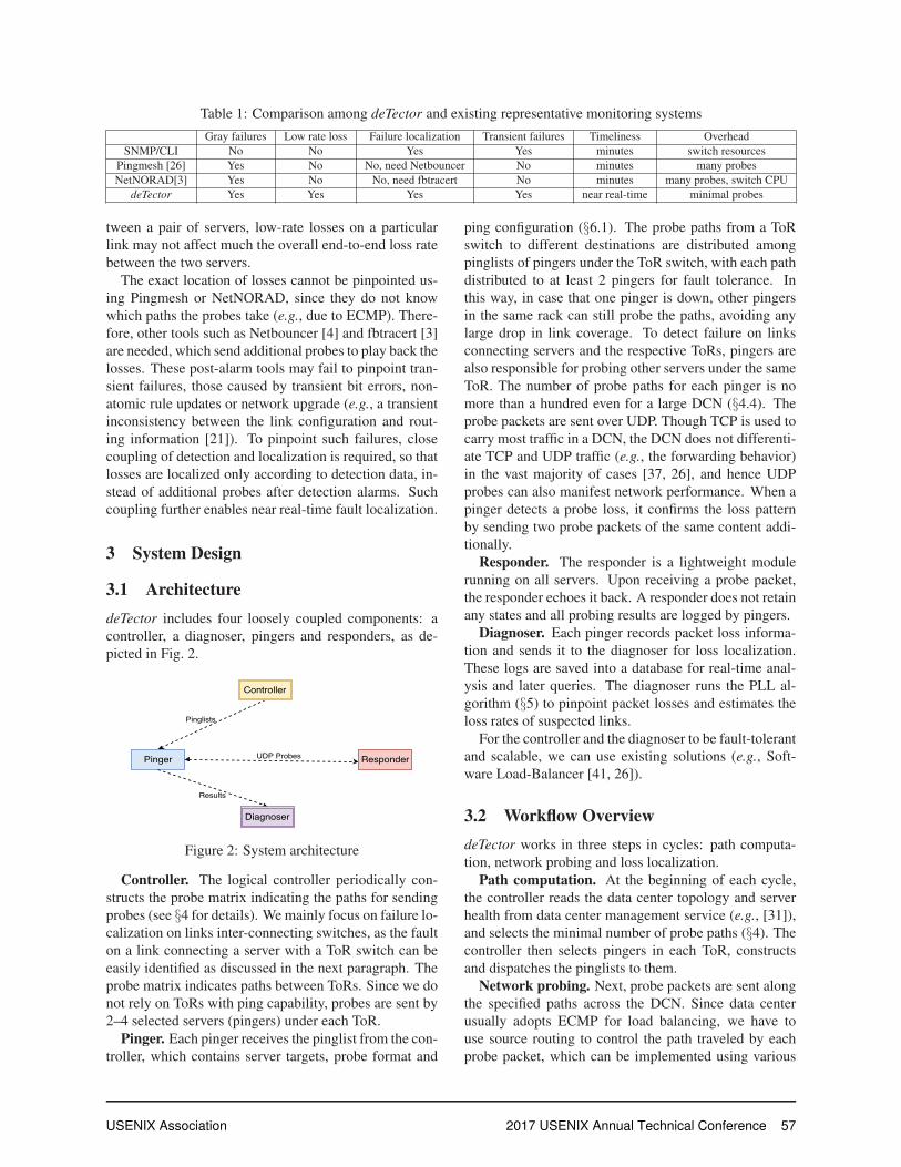
Table 1: Comparison among deTector and existing representative monitoring systems
Gray failures Low rate loss Failure localization Transient failures Timeliness Overhead
SNMP/CLI No No Yes Yes minutes switch resources
Pingmesh [26] Yes No No, need Netbouncer No minutes many probes
NetNORAD[3] Yes No No, need fbtracert No minutes many probes, switch CPU
deTector Yes Yes Yes Yes near real-time minimal probes
tween a pair of servers, low-rate losses on a particular
link may not affect much the overall end-to-end loss rate
between the two servers.
The exact location of losses cannot be pinpointed us-
ing Pingmesh or NetNORAD, since they do not know
which paths the probes take (e.g., due to ECMP). There-
fore, other tools such as Netbouncer [4] and fbtracert [3]
are needed, which send additional probes to play back the
losses. These post-alarm tools may fail to pinpoint tran-
sient failures, those caused by transient bit errors, non-
atomic rule updates or network upgrade (e.g., a transient
inconsistency between the link configuration and rout-
ing information [21]). To pinpoint such failures, close
coupling of detection and localization is required, so that
losses are localized only according to detection data, in-
stead of additional probes after detection alarms. Such
coupling further enables near real-time fault localization.
3 System Design
3.1 ArchitecturedeTector includes four loosely coupled components: a
controller, a diagnoser, pingers and responders, as de-
picted in Fig. 2.
Figure 2: System architecture
Controller. The logical controller periodically con-
structs the probe matrix indicating the paths for sending
probes (see §4 for details). We mainly focus on failure lo-
calization on links inter-connecting switches, as the fault
on a link connecting a server with a ToR switch can be
easily identified as discussed in the next paragraph. The
probe matrix indicates paths between ToRs. Since we do
not rely on ToRs with ping capability, probes are sent by
2–4 selected servers (pingers) under each ToR.
Pinger. Each pinger receives the pinglist from the con-
troller, which contains server targets, probe format and
ping configuration (§6.1). The probe paths from a ToR
switch to different destinations are distributed among
pinglists of pingers under the ToR switch, with each path
distributed to at least 2 pingers for fault tolerance. In
this way, in case that one pinger is down, other pingers
in the same rack can still probe the paths, avoiding any
large drop in link coverage. To detect failure on links
connecting servers and the respective ToRs, pingers are
also responsible for probing other servers under the same
ToR. The number of probe paths for each pinger is no
more than a hundred even for a large DCN (§4.4). The
probe packets are sent over UDP. Though TCP is used to
carry most traffic in a DCN, the DCN does not differenti-
ate TCP and UDP traffic (e.g., the forwarding behavior)
in the vast majority of cases [37, 26], and hence UDP
probes can also manifest network performance. When a
pinger detects a probe loss, it confirms the loss pattern
by sending two probe packets of the same content addi-
tionally.
Responder. The responder is a lightweight module
running on all servers. Upon receiving a probe packet,
the responder echoes it back. A responder does not retain
any states and all probing results are logged by pingers.
Diagnoser. Each pinger records packet loss informa-
tion and sends it to the diagnoser for loss localization.
These logs are saved into a database for real-time anal-
ysis and later queries. The diagnoser runs the PLL al-
gorithm (§5) to pinpoint packet losses and estimates the
loss rates of suspected links.
For the controller and the diagnoser to be fault-tolerant
and scalable, we can use existing solutions (e.g., Soft-
ware Load-Balancer [41, 26]).
3.2 Workflow OverviewdeTector works in three steps in cycles: path computa-
tion, network probing and loss localization.
Path computation. At the beginning of each cycle,
the controller reads the data center topology and server
health from data center management service (e.g., [31]),
and selects the minimal number of probe paths (§4). The
controller then selects pingers in each ToR, constructs
and dispatches the pinglists to them.
Network probing. Next, probe packets are sent along
the specified paths across the DCN. Since data center
usually adopts ECMP for load balancing, we have to
use source routing to control the path traveled by each
probe packet, which can be implemented using various
USENIX Association 2017 USENIX Annual Technical Conference 57

methods.1 A general and feasible solution is to employ
packet encapsulation and decapsulation to create end-to-
end tunnels, though it may cause encapsulating packets
twice in virtualized networks created by VXLAN [1] or
NVGRE [2]. Take the Fattree network in Fig. 1 as an
example: fixing a core switch, there is only one path be-
tween two inter-pod servers; we can use IP-in-IP encap-
sulation to wrap the probe on a server; after the packet ar-
rives at the core switch, the outer header is removed and
the packet is routed to the real destination. Such a source
routing mechanism incurs little overhead on servers and
core switches.
Loss localization. The probe loss measurements are
aggregated and analyzed by our loss localization algo-
rithm (§5) on the diagnoser. We pinpoint the faulty links,
estimate the loss rates, and send alerts to the network op-
erator for further action (e.g., examining switch logs).
4 Probe Matrix Design
The main limitation of existing monitoring systems is
that the probe path selection is far from optimum, such
that not enough useful information can be collected and
additional probes are needed to reproduce losses for lo-
calization. In this section, we elaborate how we carefully
select probe paths to overcome such a limitation.
4.1 Problem
Consider a data center network graph G = (V,E), where
V is the set of switches and E is the set of links. R is the
m×n routing matrix defined by
Ri, j =
{1 if link j is on path i0 otherwise
where m is the number of paths and n = |E| is the num-
ber of links. The possible paths and the routing matrix
are decided by the routing protocols employed in the data
center, e.g., ECMP is typically used to exploit k2/4 paral-
lel paths between any two ToRs in a k-ary Fattree. Fig. 3
gives a routing matrix R with 3 paths and 3 links. Note
that each link in a DCN is typically bi-directional. Once
we select a path from server s1 to server s2 and send a
probe, the reverse path from s2 to s1 is automatically se-
lected, since the response packet can probe faults along
the reverse direction. When we identify that link AB has
failed, it implies that the failure may lie in either direc-
tion of the link, switch A, or switch B.
1Source routing protocols have been designed in some DCNs like
BCube [24] and DCell [25]; [30, 32] introduce other solutions for ex-
plicit path control.
R =
⎛⎝
l1 l2 l3p1 1 1 0
p2 1 0 1
p3 0 0 1
⎞⎠ → R’ =
⎛⎝
l1 l2 l3 l12 l13 l23
1 1 0 1 1 1
1 0 1 1 1 1
0 0 1 0 1 1
⎞⎠
Figure 3: Extend routing matrix with virtual links
Problem 1 Given a DCN routing matrix R, select a setof paths to construct a probe matrix P, such that P si-multaneously (1) minimizes the number of paths, andachieves (2) α-coverage and (3) β -identifiability.
Minimizing the number of probe paths is desirable for
minimizing network bandwidth consumption and anal-
ysis overhead, such that we may finish probing and di-
agnosing the entire DCN in merely a few minutes. Un-
der the same probing bandwidth budget, it allows each
pinger to probe the same set of paths more frequently.
α-coverage requires that each link is covered by at
least α paths in the probe matrix. Covering a link multi-
ple times brings higher statistical accuracy for loss detec-
tion, as well as better resilience to pinger failures (since a
link is more likely to be covered by probes from multiple
pingers).
β -identifiability states that the simultaneous failures of
any (no more than) β links in the DCN can be localized
correctly. For the routing matrix in Fig. 3, suppose we
select p1 and p2 to constitute the probe matrix, i.e., the
probe matrix contains the first two rows of R. If 2 or
more links fail simultaneously, the faulty links cannot be
correctly identified, as the observation from the end is
the same, i.e., packet losses are observed on both paths.
On the other hand, if only one link is faulty, the bad link
can be identified effectively: losses are observed on both
paths, p1, or p2 if link 1, 2, or 3 is faulty, respectively.
Therefore, the probe matrix achieves 1-identifiability, but
not 2 or higher identifiability. Better identifiability con-
tributes to higher accuracy of loss localization.
We find that Problem 1 is NP-hard for general DCNs
as the Minimum Set Cover Problem is a special case of
the problem. We hence resort to an approximation algo-
rithm to compute the probing path, which is at the heart
of deTector.
4.2 PMC AlgorithmWe extend a well-known greedy algorithm [13] for con-
structing a probe matrix achieving 1-identifiability to one
achieving β -identifiability, as well as α-coverage using
a minimal number of probe paths.
In a probe matrix, a link belongs to a set of paths. To
achieve 1-identifiability, the path sets of different links
should all be different, so that losses can be observed on
a particular set of paths to identify the faulty link. Recall
that the set of links in our DCN is E. Once we select
a path from the set of all feasible paths decided by the
58 2017 USENIX Annual Technical Conference USENIX Association

routing matrix based on some criterion, it splits E into
two subsets E1 and E2, containing links on the selected
path and the other links, respectively. If we do not ob-
serve any packet loss on this path, it implies that all links
in E1 are good; otherwise, there must be at least one bad
link in E1. Similarly, we select another path to further
split E1 and E2 into smaller subsets, and repeat this pro-
cedure. Eventually if we can obtain subsets each con-
taining only one link, then the probe matrix constructed
using the selected paths achieves 1-identifiability (since
the set of paths traversing each link is unique); other-
wise, there does not exist a 1-identifiable probe matrix in
the DCN. Throughout the process, if we always select a
path whose links are present in the largest number of link
sets to further split the link sets as much as possible, we
will end up with the minimal number of paths needed.
To achieve β -identifiability, we expand the DCN
graph G with “virtual links”. A virtual link is a com-
bination of multiple physical links, and the set of paths a
virtual link belongs to can be computed by “OR”-ing to-
gether the paths including the individual links [13]. For
the example in Fig. 3, the original routing matrix R is
extended to R’ with three additional virtual links l12, l13
and l23 added; the column corresponding to the virtual
link l12 can be computed by “OR”-ing the two columns
corresponding to links l1 and l2. For β -identifiability,
∑2≤i≤β
C(|E|, i) virtual links should be added in the DCN
graph (routing matrix), corresponding to all combina-
tions of 2 to β links in the original graph. Then we can
run the above algorithm for constructing 1-identifiable
matrix based on the new routing matrix, and the result-
ing probe matrix achieves β -identifiability.
The probe matrix does not achieve even path coverage
among the links yet. For example, for a 1-identifiable
probe matrix constructed on a 64-ary Fattree, the gap
between the maximal and minimal numbers of probing
paths passing through any two links can be as large as
188. To achieve better evenness (i.e., spreading paths and
thus probe overhead evenly among the physical links),
we introduce a link weight w[link], denoting the num-
ber of paths that the link resides on, and ensure that it is
no smaller than α for any physical link. We also define
a score for each (extended) path, i.e., the path includes
virtual links from the extended routing matrix R’:
score(path) = ∑link∈path
w[link]−# of link sets on path
(1)
Here the link sets are the split link sets produced by the
procedure above. We say that a link set is on a path if the
link set contains at least one (physical or virtual) link of
the path. Thus, a lower score indicates that the links on
the path are not covered much by paths already selected
and/or more link sets can be split if the path is selected
Algorithm 1 Probe Matrix Construction (PMC) Algo-
rithm
Require: R, α , β1: Initialize w, score to 0, setnum to 1, sel paths to /0
2: R’← LINKOR(R,β )3: paths← all paths in R’, physlinks← E4: while (setnum �= |E| ‖ physlinks �= /0) && paths �= /0
do5: for path ∈ paths do6: update score[path] according to (1)
7: path← argminpath′∈paths score[path′]8: sel paths← sel paths∪{path}9: paths← paths/{path}
10: for physlink on path do11: w[physlink]← w[physlink]+1
12: if w[physlink]> α then13: physlinks← physlinks/{physlink}14: update setnum as the total number of link sets
after split by path15: return probe matrix constructed by paths in sel paths
(retaining only physical links on the paths)
in the above procedure. We strive to achieve better even-
ness among the links while guaranteeing α-coverage, by
always selecting a path with the lowest score.
Our Probe Matrix Construction algorithm, PMC, is
summarized in Alg. 1. We first reduce the problem of
constructing a β -identifiable matrix to one constructing
1-identifiable matrix, by adding virtual links to the orig-
inal routing matrix of the DCN graph (line 2, where
LINKOR denotes the method for extending routing ma-
trix discussed above). Then in each iteration we update
the score of each (extended) path (lines 5-6) and select
a path which has the minimal score among all candi-
date paths (lines 7-8). We remove the selected path from
the candidate path set (line 9), and update the weight of
physical links (w[physlink]) on the selected path (lines
10-11) and the total number of link sets that the already
selected paths can split into (line 14, which corresponds
to the procedure discussed in the second paragraph of
this subsection). If the number of paths that cover one
(physical) link exceeds α , we remove the link from the
set of all links (line 12-13). The loop stops when the
probe matrix achieves α-coverage (i.e., the set physlinksis empty) and β -identifiability (i.e., the number of link
sets split equals the number of links), or there are no
more candidate paths (i.e., the set paths is empty).
Theorem 1 The PMC algorithm achieves (1− 1e ) ap-
proximation of the optimum in terms of the total numberof probe paths selected, where e is natural logarithm.
We can prove Theorem 1 by showing that the score
of a path set is monotone, submodular and non-negative.
USENIX Association 2017 USENIX Annual Technical Conference 59

The detailed proof is in the technical report [7]. In prac-
tice, the PMC algorithm performs much better than the
(1− 1e ) ≈ 0.63 approximation ratio (§4.4). The issue of
this algorithm, however, is the computation time. The
time complexity of the algorithm is O(m2), where m is
the number of paths, since in the worst case we may up-
date the scores of all paths in each iteration and end up
with selecting all paths. In a 64-radix Fattree, there are
about 4.3×10⁹ desirable paths among ToRs. As we will
see in §4.4, the algorithm is still too slow for any data
center at a reasonable scale, and we adopt a number of
optimizations to further speed it up.
4.3 Algorithm SpeedupTo speed up the PMC algorithm, we apply several opti-
mizations based on the following three observations.
Observation 1 Problem 1 can be divided into a series ofsubproblems.
We can construct a bipartite graph according to the rout-
ing matrix: one partition corresponds to paths and the
other consists of links; an edge exists between a path
node and a link node if the link is on the path. We observe
that if the routing matrix can be partitioned into sets of
paths with no links in common, then the problem can be
divided into independent subproblems. For example, in
Fig. 1, paths traversing the red link have no link overlap-
ping with paths traversing the blue link. Therefore, the
bipartite graph can typically be divided into connected
subgraphs and each subgraph represents a smaller rout-
ing matrix and hence a subproblem. Finding connected
subgraphs can be done in linear time by traversing the
bipartite graph once. Then the PMC algorithm can be
applied to the subproblems in parallel.
Observation 2 The score of each path is non-decreasingover all iterations.
It can be proved that the score of a path is non-decreasing
(Appendix A in [7]). Inspired by the CELF algorithm for
outbreak detection in networks [38], we adopt a strategy
called lazy update which defers the update of a path score
as much as possible even though we know the score is
outdated. Specifically, we maintain a min-heap for all
paths with scores as the keys and only update the score
of a path when the path is at the top of the heap. After
score update, if the path still stays at the top of the heap,
i.e., the path has the minimal score among all available
paths, we will select the path as a probe path, even though
some path scores have yet to be updated. The correctness
of this heuristic is guaranteed by submodularity of the
score of a path set: the marginal gain provided by a path
selected in the current iteration can not be larger than that
provided by the path in the previous iteration.
Observation 3 The DCN topology is typically symmet-ric.
Due to symmetry, when a path is selected, all its topo-
logically isomorphic paths can be selected. For example
in Fig. 1, if the dashed green path spanning Pod 1 and
Pod 2 is selected, then the dashed purple path spanning
Pod 3 and Pod 4 may be a good choice too. This helps us
reduce the scale of the problem since the routing matrix
R can be reduced to a smaller matrix by excluding paths
that are topologically isomorphic to other paths. For ex-
ample, if the green path is in the matrix, we do not need
to include the purple path. For this purpose, we first need
to compute the symmetric components in a DCN graph.
There are many fast algorithms available for symmetry
discovery [17, 15], e.g., O2 [15] can finish computation
within 5 seconds for a Fattree(100) DCN, and we only
need to precompute it once for a DCN.
4.4 Performance
We run our PMC algorithm on a Dell PowerEdge R430
rack server with 10 Intel Xeon E5-2650 CPUs and 48GB
memory, to test its running time and number of paths se-
lected. We compare results on three well-known DCNs,
Fattree [9], VL2 [22] and BCube [24].2
Running time. Table 2 shows the algorithm run-
ning time for constructing a probe matrix achieving 2-
coverage and 1-identifiability. The strawman approach is
our PMC algorithm without any optimizations. The last
three columns contain results when the respective opti-
mization is in place (in addition to the previous one(s)).
The results show that PMC can efficiently select probe
paths for very large DCNs. Specifically, without algo-
rithm speedup, the computation time of PMC can be
larger than 24 hours; after each optimization, the time de-
creases significantly and we can compute the probe ma-
trix for Fattree(72), VL2(140,120,100) and BCube(8,4)
within 18 seconds, 86 seconds and 70 seconds, respec-
tively. We note that the running time in case of problem
decomposition for VL2 and BCube is a bit longer than
that of strawman. This is because decomposition does
not apply to the two DCN topologies, but we need extra
time to decide whether the matrix is decomposable.
Path number. Table 3 shows the number of selected
paths with different α and β in different DCNs. Com-
pared with the number of original paths in DCNs, PMC
only selects a small percentage of paths. We can prove
that the least number of paths for achieving 1-coverage
and 1-identifiability is k3/5 for any k-ary Fattree (Ap-
pendix B in [7]). Thus, a Fattree(64) DCN needs at least
52428 paths and our algorithm selects slightly more, i.e.,
2BCube is a server centric architecture and we treat servers as
switches to run our algorithm.
60 2017 USENIX Annual Technical Conference USENIX Association

Table 2: Algorithm running time (seconds) with α = 2,β = 1 in different DCNs
DCNs # of nodes # of links # of original paths Strawman Decomposition Lazy update Symmetry reduction
Fattree(12) 612 1296 184,032 231.458 5.216 0.506 0.126
Fattree(24) 4,176 10,368 11,902,464 > 24h 1381.226 23.254 0.280
Fattree(72) 99,792 279,936 8,703,770,112 > 24h > 24h > 24h 17.054
VL2(20, 12, 20) 1,282 1,440 70,800 22.030 23.126 0.77 0.253
VL2(40, 24, 40) 9,884 10,560 4,588,800 7387.412 7470.476 39.028 1.404
VL2(140,120,100) 424,390 436,800 4,938,024,000 > 24h >24h >24h 85.567
BCube(4, 2) 112 192 12,096 4.871 4.936 0.227 0.117
BCube(8, 2) 704 1,536 784,896 4050.776 4390.168 9.854 0.220
BCube(8, 4) 53,248 163,840 5,368,545,280 > 24h > 24h > 24h 69.778
Table 3: Number of selected paths with different (α ,β )
DCNs Original pathsSelected paths with (α,β )(1, 0) (1, 1) (3, 2)
Fattree(32) 66,977,792 4,096 7,680 12,288
Fattree(64) 4,292,870,144 32,768 61,440 98,304
VL2(72,48,40) 107,371,008 864 1,440 2,640
VL2(128,96,80) 2,415,132,672 3,072 5,760 9,216
BCube (8,2) 784,896 1,712 2,016 2,832
BCube (8,4) 5,368,545,280 49,152 70,572 119,556
61440 paths. This implies that pingers under each se-
lected ToR in the Fattree are only responsible for probing
about 60 paths, much fewer than that of Pingmesh (about
2000-5000 paths). We also find that VL2 requires much
fewer paths than Fattree and BCube. This is because VL2
has a much smaller number of links between switches
(12288 links in VL2(128, 96,80)), as compared to Fat-
tree (131072 links in Fattree(64)) and BCube (163840
links in BCube(8,4)).
Note that the number of selected path may change
when the third optimization, based on topology symme-try, is in place. Our evaluation shows that the number of
selected paths with symmetry reduction is very similar to
that without symmetry reduction. This is consistent with
the result in [30], and we hence omit the analysis.
Results for β ≥ 3. The probe matrices we constructed
above achieve at most 2-identifiability. For β ≥ 3, the
computation of PMC is not efficient in large DCNs. For
the example of a 48-ary Fattree, computing a probe ma-
trix achieving 3-identifiability requires at least 24 hours,
even when we apply all speedup optimizations in §4.3.
The fundamental reason is that the routing matrix R be-
comes much larger when the number of column increases
from n to ∑1≤i≤β
C(n, i), by adding virtual links. However,
surprisingly, we find that 2-identifiability is enough for
loss localization in DCNs, as we will see in §6.4.
5 Loss Localization
5.1 Data Pre-processing
After collecting the probe data, the first step is to pre-
process the data, removing outliers and normal cases.
Severe packet losses could be caused by bad pingers and
responders (e.g., the server is down or was rebooting dur-
ing probing, thus causing many false alarms [37]). Such
outliers can be identified by keeping track of the status
of servers using a watchdog service. In addition, a link
normally has a regular low loss rate, e.g., 10−4–10−5,
due to transient congestion, bit errors, which should not
be considered as failures [26]. To exclude such nor-
mal cases, we filter out paths with extremely low packet
loss rates by setting a threshold on the number of packet
losses in a period of time or on packet loss ratio (e.g.,10−3 [26, 21]).3 After pre-processing, the loss data that
remain (in the form of (path, number o f losses)) are
likely manifest of network failures rather than noises.
5.2 ProblemOur fault localization problem is: given end-to-end
packet loss observations, find the smallest set of faulty
links that best explains the observations. This problem is
NP-hard as it can be reduced to the NP-complete Min-
imum Hitting Set Problem [18]. Besides, we face two
challenges not existed in previous work:
Much larger problem scale. Our study focuses
on large-scale DCN networks, different from smaller
networks investigated in the existing loss localization
work [10, 18, 42]. At our problem scale, the existing
algorithms are not fast enough (taking tens of seconds or
even minutes) for real-time loss localization.
Different loss patterns. Network failures are mainly
exhibited as two kinds of packet losses: full packet loss
and partial packet loss, meaning that all or part of the
packets traversing a link are dropped. Existing tomog-
raphy techniques assume that if all links on a path are
good, then the path is good [19]. This is not true in case
of partial packet loss in data centers, e.g., packet black-
hole may lead to losses on a link only for a subset of
paths using that link.
5.3 PLL AlgorithmBased on the Tomo algorithm in [18], we design an effi-
cient Packet Loss Localization algorithm, PLL, to local-
3To avoid inaccuracy of the threshold approach, we can use statis-
tical hypothesis testing to look at loss rates over time for noisy data
filtering [27].
USENIX Association 2017 USENIX Annual Technical Conference 61

ize packet losses in DCNs (see [7] for more details). The
basic idea of PLL is as follows.
Step 1: Divide the problem into a series of subprob-
lems, by decomposing the probe matrix following the
same steps discussed for decomposing the routing matrix
in §4.3. For each subproblem, run the following steps.
Step 2: If all probe paths traversing a link experience
no packet loss, we exclude the link. For the remaining
links, we calculate a hit ratio for each link, i.e., the ratio
of the number of observed lossy paths through the link
over the number of all probe paths using the link [34].
Step 3: We compute a score for each link as the num-
ber of lost packets that the link can explain, i.e., if a link
lies in the packet path, we say the link can explain the
packet loss.
Step 4: Among those links whose hit ratios are larger
than a preset threshold, we greedily select the link with
the maximal score and remove those losses this link can
explain.
Step 5: Repeat Step 3 and Step 4 until no loss remains
unexplained.
PLL differs from Tomo mainly in handling partial
packet losses, i.e., we use a hit ratio threshold to filter
suspected links. Setting the threshold requires network
operator’s experience and, if possible, by learning from
real loss data. The analysis on setting this threshold is
presented in [7] due to space constraint and we set it to
0.6 by default in our experiments.
We have compared performance of PLL and other ex-
isting loss localization methods (e.g., Tomo, SCORE [34]
and OMP [42]), and present the results in [7]. The results
show that given the same probe matrix, PLL achieves 2%
higher accuracy (defined as true positive ratio, i.e., the
percentage of bad links correctly identified as bad over
all truly bad links), 2% lower false positive ratio (i.e.,the percentage of good links incorrectly identified as bad
over all correctly and incorrectly identified links), and
is an order of magnitude faster (e.g., localizing failures
within 1 second in a large DCN with 82944 links) than
the other algorithms.
6 Implementation and Evaluation
6.1 ImplementationWe run the controller on one Dell server (or it can run in
a distributed fashion over multiple servers for large-scale
networks). A watchdog service also runs on the server
for monitoring the health of other servers and removing
bad ones. The controller runs the PMC algorithm to re-
compute the probe matrix every 10 minutes, based on the
current network topology from the watchdog service.4
4Once a link or a switch has failed, we remove related link(s) from
the routing matrix to avoid selecting bad paths for probing. Note that
The computed probe matrix is divided into XML pinglist
files for dispatching to pingers. A pinglist file contains
file version, the pinger’s IP address, IP addresses of re-
sponders, transport port numbers, the packet-sending in-
terval and IP addresses of core switches. Our measure-
ment shows that the controller can handle 4473 pinglist
requests per second on average with maximal bandwidth
consumption 688.56Mb/s using one core. Since pingers
are deployed on a small number of servers (about 10%
among all servers), the controller can support more than
100,000 pingers by slightly randomizing the time when
pingers request for pinglists in each cycle.
Each pinger implements a communication module and
a probing module. The communication module is re-
sponsible for connections with the controller and the di-
agnoser. It fetches the pinglist file from the controller
by an HTTP GET request in every cycle (i.e., 10 min-
utes). The probing module generates probe packets ac-
cording to the pinglist and encapsulates them by IP-in-IP
(§3.1). In our experiments, a pinger loops over a range
of ports for each path, and emits several packets for ev-
ery port. Each probe packet has an average size of 850
Bytes, carrying a specified DSCP value in the IP header
to test different QoS classes [12]. If there is no response
for a probe within 100ms, we mark it as a loss. A pinger
repeatedly sends packets by looping through the paths in
the pinglist for multiple times (for statistical accuracy),
at the rate of 10 packets per second. Every 30 seconds,
the pinger aggregates the probing results (i.e., the number
of packet losses and the number of packets sent on each
probe path) into an XML file and sends it to the diagnoser
by an HTTP POST request. The responder module runs
in the userspace of all servers, which listens to a particu-
lar port, and upon packet arrival, it adds a timestamp and
sends the packet back. The pinger and responder incur
little overhead on servers, as we will see in §6.3.
The diagnoser is a Web server module running on the
same server where the controller is in our experiments. It
runs the PLL algorithm for fault localization once every
half a minute, using collected probe results in the past
30 seconds. Given the limited number of servers in our
testbed, we run a virtual machine to emulate a server.
6.2 Experiment SetupWe build a 4-ary Fattree testbed with 20 ONetSwitch [5,
29, 28], each equipped with FPGA-based hardware re-
configurable dataplane, four 1GbE ports and one ded-
icated management port. Though we do not require
programmable switches in deTector, employing SDN
switches facilitates our emulation of various failure cases
that may happen in a real-world DCN. Specifically, we
categorize all losses into three types:
it does not affect symmetry computation which only pre-runs once on
the original DCN topology.
62 2017 USENIX Annual Technical Conference USENIX Association

Full packet loss. We install OpenFlow rules with high
priority to drop all packets coming from a particular port,
to emulate a faulty link with full packet loss. To emulate
a switch down case, we install rules to drop all packets at
the switch.
Deterministic partial loss. Packets with certain fea-
tures (e.g., specific IPs, port numbers) may be dropped
on a link deterministically, e.g., in case of packet black-
hole or misconfigured routing rules. To emulate such
failures, we install rules on the switches to match and
drop packets with certain headers.
Random partial loss. Sometimes packets on a link
are dropped randomly, as caused by bit flips, CRC er-
rors, buffer overflow, etc. SDN switches do not support
random packet dropping. To emulate such losses, we in-
stall rules on the switches to redirect all packets on an
emulated bad link to the SDN controller, and the SDN
controller drops the received packets with certain proba-
bility, following the pattern extracted from [12].
Due to no access to loss data in real-world data centers,
we produce the above loss types according to the failure
measurements in [20] and traffic measurements in [12].
Specifically, we set parameters such as link vs. switch
failure percentage, link loss rates (ranging from 10−4 to
1), failure probabilities for switches in different tiers, all
based on the above measurements. The loss distribu-
tion for links in different tiers is extracted from Fig. 3
in [12]. Aside from deTector, we also implement the
probing modules of Pingmesh and NetNORAD on our
testbed for performance comparison, as well as their fail-
ure localization tools, Netbouncer and fbtracert. Since
we do not know some of their implementation details
(e.g., how data pre-processing is done), we implement
those details in the same way across all three systems.
6.3 Performance
We first investigate how probing itself affects the whole
DCN. We use realistic packet traces (including informa-
tion such as packet header, timestamp) from a univer-
sity data center [11] (mostly HTTP flows) to generate
workload traffic in our testbed, where each server con-
tinuously replays flows based on the packet traces and
sends them to a random receiver. We evaluate how our
probing frequency (i.e., the number of probes a pinger
sends per second) affects the performance of the PLL al-
gorithm, the overhead on the pinger, and RTT and jitter
experienced by the workload traffic. In each minute of
our experiment, we emulate a failure randomly picked
among the three types of failures, with the failed switches
or links randomly picked in the DCN. We run our exper-
iment for 2000 minutes and obtain the average results.
Fig. 4 shows that a higher probe sending frequency
leads to a higher accuracy and a lower false positive ra-
(a) Performance of PLL (b) CPU, memory and band-
width overhead on pingers
(c) RTT of workload traffic (d) Jitter of workload traffic
Figure 4: Sensitivity test of sending frequency
tio (Fig. 4(a)), but causes higher CPU utilization and
bandwidth consumption on pingers (Fig. 4(b)) as well
as slightly larger fluctuation of the RTT (Fig. 4(c)) and
jitter (Fig. 4(d)) experienced by the workload. We find
that 10–15 probes per second is good enough since we
can still achieve higher than 95% accuracy and a lower
than 3% false positive ratio, while only consuming about
100Kbps bandwidth, 0.4% CPU and 13MB memory on
each pinger. Besides, it does not introduce apparent de-
lay and jitter variations for workload traffic. Note that the
overhead of a responder is much smaller than a pinger
because it resumes fewer tasks (e.g., no communication
with the controller and the diagnoser), and hence the re-
sults are omitted.5 In all our experiments, the pinger
sends 10 packets per second by default (i.e., the red
square in Fig. 4).
We then compare the accuracy, false positive ratio and
overhead among deTector, Pingmesh and NetNORAD.
Since Pingmesh can not localize failures by itself, once it
detects a suspected source-destination server pair, we use
Netbouncer [4] to go through all possible paths between
this server pair for loss localization. As for NetNORAD,
similarly, we use fbtracert [3] to probe all possible paths
between the suspected server pair. The interval of loss
data collection is 30 seconds for three systems.
Fig. 5 shows the comparison when one failure is emu-
lated in the testbed (the failure is randomly picked as in
the previous experiment). The number of (ping and re-
ply) probes in the figure includes probes sent for detec-
tion and probes for localization (if any) in each minute
of the experiment. More probes indicate not only more
5Even when we place the pinger and responder on the same server,
the overhead is negligible.
USENIX Association 2017 USENIX Annual Technical Conference 63

Figure 5: Accuracy and false positives of three monitor-
ing systems with different number of probes per minute
Figure 6: Results comparison with multiple failures
bandwidth consumption, but also higher CPU and mem-
ory usage. For deTector, we use a probe matrix with 1-
identifiability and 3-coverage (since it is impossible to
achieve 2-identifiability in a 4-ary Fattree). As we can
see, deTector achieves high accuracy and a low false pos-
itive ratio with a much smaller number of probes, be-
cause deTector covers more types of losses (e.g., low rate
loss) and takes carefully planned paths. For instance, to
achieve 98% accuracy and 1% false positives, deTector,
NetNORAD and Pingmesh need to send 7200, 20700
and 35100 probes per minute, respectively. When the
probe overhead is same (same number of probes sent per
minute), the accuracy and false positive ratio achieved
by deTector is better than those of NetNROAD; as com-
pared to Pingmesh, the accuracy of deTector is much bet-
ter, while the false positive ratio of Pingmesh is slightly
smaller sometimes, since it possibly probes all paths.
Fig. 6 further shows the accuracy and false positive
ratio with multiple failures, when the probe overhead is
fixed to be the same, i.e., 5850 probes per minute. de-Tector always achieves much better performance than
Pingmesh and NetNORAD. Note that deTector also de-
tects and localizes failures much faster than NetNORAD
and Pingmesh (30 seconds in advance in our experi-
ments), because deTector does not need any other diag-
nosis tools to send an additional round of probes for loss
localization, while others do.
6.4 SimulationWe supplement our experimental evaluation with simula-
tions, to investigate how identifiability of the probe ma-
Table 4: Accuracy in a 18-radix Fattree, with probe ma-
trices of different levels of coverage and identifiability
(α,β ) # of pathsAccuracy (%) with # of failed links
1 5 10 20 50
(1,0) 729 30.56 30.87 30.30 30.26 29.19
(2,0) 1485 58.43 57.43 57.08 56.81 57.11
(3,0) 2187 68.22 70.61 69.89 70.40 70.14
(1,1) 1269 94.74 93.37 94.21 93.43 90.29
(1,2) 1512 99.26 99.06 99.02 98.77 95.92
(1,3) 2349 99.63 99.63 99.67 99.62 98.07
trix influences the accuracy of our failure localization,
when running deTector in larger Fattree networks.
We first vary α and β for probe matrix construction
in an 18-radix Fattree. Table 4 shows that higher cov-
erage and higher identifiability lead to higher accuracy,
while the overhead (i.e., the number of selected paths)
does not increase much. Also, we find that identifiability
is more effective and desirable than coverage for failure
localization, since a 1-identifiability matrix increases the
accuracy a lot (from one with 0-identifiability guarantee),
with much less overhead than a 3-coverage probe matrix.
Note that further increasing the level of identifiability
for β > 1 does not increase the accuracy much, and probe
matrices achieving 1-identifiability can already lead to
higher than 90% accuracy. According to the measure-
ments in [12], less than 10% failure events (failures oc-
curring concurrently) contain more than four failures and
less than 1% failure events contain more than 20 failures.
This implies that a probe matrix with 1-identifiability
can guarantee higher than 93% accuracy for 90% fail-
ure events and 2-identifiability provides a 98% accuracy
for 99% failure events.
The result is surprising but reasonable: Since we use
a number of optimizations (§4.3) to reduce the size of
the routing matrix, the PMC algorithm in fact achieves
β ′-identifiability (where β ′ is larger than β used in
the algorithm) for the whole probe matrix, rather than
β -identifiability computed for each small probe matrix
(corresponding to a small network topology). Therefore,
deTector may fail to localize all failures only if more
than β failures appear in a small topology, which occurs
with relatively low probability. This shows that using a
probe matrix with a low level of identifiability guaran-
tee is good enough to identify a much larger number of
concurrent failures.
In addition, by examining the failure events that deTec-tor fails to localize with a low identifiability probe ma-
trix but can identify using a high identifiability matrix,
we find that higher identifiability achieves better results
only when the number of simultaneously failed links is
very large. Such a failure event with many concurrent
link failures is usually triggered by a common bug in
practice (e.g., 180 links fail simultaneously due to sched-
uled maintenance to multiple aggregation switches [20]),
64 2017 USENIX Annual Technical Conference USENIX Association

Table 5: Fault localization performance with probe ma-
trix of 2-identifiability in a 48-ary Fattree
# of failed links 1 5 10 20 50
Accuracy (%) 98.95 98.99 98.98 98.93 98.87
False positive (%) 0.01 0.02 0.02 0.02 0.02
False negative (%) 1.05 1.01 1.02 1.07 1.13
and thus those faulty links are spatially clustered. In such
cases, operators can locate the failure spot effectively ac-
cording to the positions of most failed links.
We further examine the fault localization accuracy,
false positive and false negative (bad links incorrectly
identified as good) ratios achieved using a probe matrix
of 2-identifiability in a 48-ary Fattree. Table 5 shows that
the false positive and false negative ratios remain in a
very low level. In particular, the false positive rate is ex-
tremely low (< 1%), which is desirable in practice [18].
The false negatives are mainly caused by losses of ex-
tremely low loss rate and intermittent losses which may
happen at longer intervals (than 1 minute) [23]. Since it
takes longer time to expose these losses, we can further
reduce false negatives by examining loss measurements
in larger time windows, e.g., 10 minutes.
7 Discussions
Packet entropy. deTector tries to increase packet en-
tropy (i.e., different packet patterns) by varying IP ad-
dresses, port numbers and DSCP values, to cover as
many failures as possible. However, our implementa-
tion uses IP-in-IP encapsulation for source routing, and
hence the range of destination IP addresses is somewhat
limited. In addition, since we use UDP for network
probing, deTector may not be able to detect failures re-
lated to other protocols, e.g., misconfigured TCP param-
eters [26]. Adopting other source routing solutions and
adding more protocols to increase packet entropy are part
of our future work.
Loss diagnosis. While deTector can localize where
packet drops occur, it does not know what causes the
drops, e.g., software bugs, misconfigured rules or bursty
traffic. This is a common deficiency of existing monitor-
ing systems, since network diagnosis is rather complex.
However, it is possible to distinguish full losses, deter-
ministic partial losses, random partial losses and losses
due to congestion, to narrow down the diagnosis scope
(e.g., using machine learning approaches), since they ex-
hibit different loss characteristics. We consider this as a
promising future direction to explore.
Beyond deTector. As opposed to probe-based solutions
like deTector, there are some recent efforts on embedding
metadata in the packet header to trace packet path for net-
work debugging (e.g., CherryPick [46], PathDump [47]).
Our technique can be applied to reduce the overhead in-
volved in these approaches, i.e., only packets travers-
ing those paths computed by the PMC algorithm need
to carry routing information in the packet headers.
8 Related Work
Probe design. Many existing work (e.g., [14, 18, 43, 33,
27]) exploit logs on switches, or utilize multicast or net-
work coding for network probing. Instead, we treat each
switch as a blackbox, and adopt a topology-aware end-
to-end probing approach. Some studies [16, 40, 23] es-
timate loss rates of all links, while we aim at identifying
bad links (i.e., failure spots). Zeng et al. [48] and Nico-
las et al. [23] propose monitoring solutions for backbone
networks that do not apply in DCNs due to scalability,
and the main difference lies in probe matrix design.
Fault localization. Our goal of accurately identify-
ing faulty links falls squarely in the area of binary net-
work tomography. Tomography algorithms such as Sher-
lock [10], Tomo [18], GREEDY [35], SCORE [34] and
OMP [42] do not work well for DCNs due to their prob-
lem scales and loss characteristics. Our PLL algorithm is
built on these work and conquers their limitations.
DCN monitoring. Our work mainly differs from ex-
isting monitoring systems such as Pingmesh [26] and
NetNORAD [37] in the design of probe matrix. We
argue that loss detection and localization must be cou-
pled together to localize more failures (e.g., transient fail-
ures) in real time with low overhead. Carefully designed
probe matrix is the key to achieve them. LossRadar [39]
is a switch-based solution but it requires programmable
switches. Dapper [44] and Zipkin [8] are distributed trac-
ing systems to gather timing data for root-cause analysis.
9 Conclusion
deTector is a real-time, low-overhead and high-accuracy
monitoring system for large-scale data center networks.
At its core is a carefully designed probe matrix, con-
structed by a scalable greedy path selection algorithm
with minimized probe overhead. We also design an ef-
ficient failure localization algorithm according to differ-
ent patterns of packet losses. Our analysis, testbed ex-
periments and large-scale simulations show that deTec-tor is highly scalable, practically deployable with low
overhead, and can localize failures with high accuracy
in near real time.
Acknowledgments We thank Xiaowei Wu for his help
with algorithm design. This work was supported by Na-
tional Key Research and Development Program of China
2016YFB0800101, NSFC 61672425, NSFC 61628209,
and Hong Kong RGC grants HKU 718513, 17204715,
17225516, C7036-15G (CRF).
USENIX Association 2017 USENIX Annual Technical Conference 65

References
[1] VXLAN. https://tools.ietf.org/html/
rfc7348, 2014.
[2] NVGRE. https://tools.ietf.org/html/
rfc7637, 2015.
[3] Fbtracert. https://github.com/facebook/
fbtracert, 2016.
[4] Microsoft Netbouncer. https://www.youtube.
com/watch?v=nfEOEKlInK8, 2016.
[5] ONetSwitch. http://www.onetswitch.org/
index, 2016.
[6] deTector project. https://github.com/
yhpeng-git/deTector, 2017.
[7] deTector technical report. https://github.
com/yhpeng-git/deTector/blob/master/
documentation/technical_report.pdf,
2017.
[8] Zipkin. http://zipkin.io, 2017.
[9] AL-FARES, M., LOUKISSAS, A., AND VAHDAT,
A. A scalable, commodity data center network ar-
chitecture. In Proc. of ACM SIGCOMM (2008).
[10] BAHL, P., CHANDRA, R., GREENBERG, A.,
KANDULA, S., MALTZ, D. A., AND ZHANG,
M. Towards highly reliable enterprise network ser-
vices via inference of multi-level dependencies. In
Proc. of ACM SIGCOMM (2007).
[11] BENSON, T. Data set for IMC 2010 data cen-
ter measurement. http://pages.cs.wisc.edu/
~tbenson/IMC10_Data.html, 2010.
[12] BENSON, T., ANAND, A., AKELLA, A., AND
ZHANG, M. Understanding data center traffic char-
acteristics. In Proc. of ACM SIGCOMM (2010).
[13] BRODIE, M., RISH, I., AND MA, S. Optimizing
probe selection for fault localization. In Proc. ofthe 12th International Workshop on DistributedSystems: Operations and Management (DSOM)(2001).
[14] CASTRO, R., COATES, M., LIANG, G., NOWAK,
R., AND YU, B. Network tomography: recent de-
velopments. Statistical Science 19, 3 (2004), 499–
517.
[15] CHEN, K., GUO, C., WU, H., YUAN, J., FENG,
Z., CHEN, Y., LU, S., AND WU, W. Generic and
automatic address configuration for data center net-
works. In Proc. of ACM SIGCOMM (2010).
[16] CHEN, Y., BINDEL, D., SONG, H., AND KATZ,
R. H. An algebraic approach to practical and scal-
able overlay network monitoring. In Proc. of ACMSIGCOMM (2004).
[17] DARGA, P. T., SAKALLAH, K. A., AND
MARKOV, I. L. Faster symmetry discovery using
sparsity of symmetries. In Proc. of the 45th AnnualDesign Automation Conference (DAC) (2008).
[18] DHAMDHERE, A., TEIXEIRA, R., DOVROLIS, C.,
AND DIOT, C. Netdiagnoser: Troubleshooting net-
work unreachabilities using end-to-end probes and
routing data. In Proc. of the 3rd ACM InternationalConference on emerging Networking EXperimentsand Technologies (CoNEXT) (2007).
[19] DUFFIELD, N. Network tomography of binary
network performance characteristics. IEEE Trans-actions on Information Theory 52, 12 (November
2006), 5373–5388.
[20] GILL, P., JAIN, N., AND NAGAPPAN, N. Under-
standing network failures in data centers: measure-
ment, analysis, and implications. In Proc. of ACMSIGCOMM (2011).
[21] GOVINDAN, R., MINEI, I., KALLAHALLA, M.,
KOLEY, B., AND VAHDAT, A. Evolve or die:
High-availability design principles drawn from
Google’s network infrastructure. In Proc. of ACMSIGCOMM (2016).
[22] GREENBERG, A., HAMILTON, J. R., JAIN, N.,
KANDULA, S., KIM, C., LAHIRI, P., MALTZ,
D. A., PATEL, P., AND SENGUPTA, S. VL2:
a scalable and flexible data center network. In
Proc. of ACM SIGCOMM (2009).
[23] GUILBAUD, N., AND CARTLIDGE, R. Localizing
packet loss in a large complex network. https:
//www.nanog.org/meetings/nanog57/
presentations/Tuesday/tues.general.
GuilbaudCartlidge.Topology.7.pdf, 2013.
[24] GUO, C., LU, G., LI, D., WU, H., ZHANG,
X., SHI, Y., TIAN, C., ZHANG, Y., AND LU, S.
BCube: a high performance, server-centric network
architecture for modular data centers. In Proc. ofACM SIGCOMM (2009).
[25] GUO, C., WU, H., TAN, K., SHI, L., ZHANG, Y.,
AND LU, S. DCell: a scalable and fault-tolerant
network structure for data centers. In Proc. of ACMSIGCOMM (2008).
66 2017 USENIX Annual Technical Conference USENIX Association

[26] GUO, C., YUAN, L., XIANG, D., DANG, Y.,
HUANG, R., MALTZ, D., LIU, Z., WANG, V.,
PANG, B., CHEN, H., ET AL. Pingmesh: A
large-scale system for data center network latency
measurement and analysis. In Proc. of ACM SIG-COMM, 2015.
[27] HERODOTOU, H., DING, B., BALAKRISHNAN,
S., OUTHRED, G., AND FITTER, P. Scalable near
real-time failure localization of data center net-
works. In Proc. of the 20th ACM International Con-ference on Knowledge Discovery and Data Mining(SIGKDD) (2014).
[28] HU, C., YANG, J., GONG, Z., DENG, S., AND
ZHAO, H. DesktopDC: setting all programmable
data center networking testbed on desk. ACM SIG-COMM Computer Communication Review 44, 4
(2015), 593–594.
[29] HU, C., YANG, J., ZHAO, H., AND LU, J. De-
sign of all programmable innovation platform for
software defined networking. In In Proc. of the 4thOpen Networking Summit (ONS) (2014).
[30] HU, S., CHEN, K., WU, H., BAI, W., LAN, C.,
WANG, H., ZHAO, H., AND GUO, C. Explicit path
control in commodity data centers: Design and ap-
plications. In Proc. of the 12th USENIX Symposiumon Networked Systems Design and Implementation(NSDI) (2015).
[31] ISARD, M. Autopilot: automatic data center man-
agement. ACM SIGOPS Operating Systems Review41, 2 (April 2007), 60–67.
[32] JYOTHI, S. A., DONG, M., AND GODFREY, P.
Towards a flexible data center fabric with source
routing. In Proc. of the 1st ACM SIGCOMM Sym-posium on Software Defined Networking Research(SOSR) (2015).
[33] KANDULA, S., MAHAJAN, R., VERKAIK, P.,
AGARWAL, S., PADHYE, J., AND BAHL, P. De-
tailed diagnosis in enterprise networks. In Proc. ofACM SIGCOMM (2009).
[34] KOMPELLA, R. R., YATES, J., GREENBERG, A.,
AND SNOEREN, A. C. IP fault localization via risk
modeling. In Proc. of the 2nd USENIX Symposiumon Networked Systems Design and Implementation(NSDI) (2005).
[35] KOMPELLA, R. R., YATES, J., GREENBERG, A.,
AND SNOEREN, A. C. Detection and localization
of network black holes. In Proc. of IEEE INFO-COM (2007).
[36] LAPUKHOV, P. Configuring IPSLA.
http://www.cisco.com/c/en/us/td/docs/
switches/lan/catalyst4500/12-2/44sg/
configuration/guide/Wrapper-44SG/
swipsla.html.
[37] LAPUKHOV, P. Network debugging at scale.
https://www.nanog.org/sites/default/
files/Lapukhov_Move_Fast_Unbreak.pdf,
2016.
[38] LESKOVEC, J., KRAUSE, A., GUESTRIN,
C., FALOUTSOS, C., VANBRIESEN, J., AND
GLANCE, N. Cost-effective outbreak detection in
networks. In Proc. of the 13th ACM InternationalConference on Knowledge Discovery and DataMining (SIGKDD) (2007).
[39] LIU, Y., MIAO, R., KIM, C., AND YUU, M. Loss-
Radar: Fast detection of lost packets in data center
networks. In Proc. of the 12th ACM InternationalConference on emerging Networking EXperimentsand Technologies (CoNEXT) (2016).
[40] MA, L., HE, T., LEUNG, K. K., TOWSLEY, D.,
AND SWAMI, A. Efficient identification of additive
link metrics via network tomography. In Proc. ofthe 33rd IEEE International Conference on Dis-tributed Computing Systems (ICDCS) (2013).
[41] PATEL, P., BANSAL, D., YUAN, L., MURTHY, A.,
GREENBERG, A., MALTZ, D. A., KERN, R., KU-
MAR, H., ZIKOS, M., WU, H., ET AL. Ananta:
cloud scale load balancing. In Proc. of ACM SIG-COMM (2013).
[42] PATI, Y. C., REZAIIFAR, R., AND KRISH-
NAPRASAD, P. Orthogonal matching pursuit: Re-
cursive function approximation with applications to
wavelet decomposition. In Proc. of the 27th Asilo-mar Conference on Signals, Systems and Comput-ers (ACSSC) (1993).
[43] SHARMA, G., JAGGI, S., AND DEY, B. Net-
work tomography via network coding. In Proc. ofthe 3rd Information Theory and Applications Work-shop (ITA) (2008).
[44] SIGELMAN, B. H., BARROSO, L. A., BURROWS,
M., STEPHENSON, P., PLAKAL, M., BEAVER,
D., JASPAN, S., AND SHANBHAG, C. Dapper,
a large-scale distributed systems tracing infrastruc-
ture. Tech. rep., Google, Inc., 2010.
[45] SINGH, A., ONG, J., AGARWAL, A., ANDERSON,
G., ARMISTEAD, A., BANNON, R., BOVING,
S., DESAI, G., FELDERMAN, B., GERMANO, P.,
USENIX Association 2017 USENIX Annual Technical Conference 67

ET AL. Jupiter rising: A decade of Clos topolo-
gies and centralized control in Google’s datacenter
network. In Proc. of ACM SIGCOMM (2015).
[46] TAMMANA, P., AGARWAL, R., AND LEE, M.
Cherrypick: Tracing packet trajectory in software-
defined datacenter networks. In Proc. of the 1stACM SIGCOMM Symposium on Software DefinedNetworking Research (SOSR) (2015).
[47] TAMMANA, P., AGARWAL, R., AND LEE, M.
Simplifying datacenter network debugging with
pathdump. In Proc. of the 12th USENIX Symposiumon Operating Systems Design and Implementation(OSDI) (2016).
[48] ZENG, H., MAHAJAN, R., MCKEOWN, N.,
VARGHESE, G., YUAN, L., AND ZHANG, M.
Measuring and troubleshooting large operational
multipath networks with gray box testing, msr-tr-
2015-55. Tech. rep., 2015.
68 2017 USENIX Annual Technical Conference USENIX Association