Remote Sensing of Environment 113 (2009) 1293–1303

Contents lists available at ScienceDirect

Remote Sensing of Environment

j ourna l homepage: www.e lsev ie r.com/ locate / rse

Detection of Rossby waves in multi-parameters in multi-mission satelliteobservations and HYCOM simulations in the Indian Ocean

Bulusu Subrahmanyam a,⁎, David M. Heffner b, David Cromwell c, Jay F. Shriver d

a Marine Science Program & Dept. of Geological Sciences, University of South Carolina, Columbia, SC 29205, USAb Dept. of Geological Sciences, University of South Carolina, Columbia, SC 29205, USAc Ocean Observing and Climate Research Group, National Oceanography Centre, Southampton, S014 3ZH, UKd Naval Research Laboratory, Stennis Space Center, Mississippi, USA

⁎ Corresponding author. Tel.: +1 803 777 2572; fax: +E-mail address: sbulusu@geol.sc.edu (B. Subrahman

0034-4257/$ – see front matter © 2009 Elsevier Inc. Adoi:10.1016/j.rse.2009.02.017

a b s t r a c t

a r t i c l e i n f o

Article history:Received 30 September 2008Received in revised form 6 February 2009Accepted 14 February 2009

Keywords:Rossby wavesIndian OceanHYCOMSatellite observationsSSHSSTOcean color

Rossby waves are difficult to detect with in situ methods. However, as we show in this paper, they can beclearly identified in multi-parameters in multi-mission satellite observations of sea surface height (SSH), seasurface temperature (SST) and ocean color observations of chlorophyll-a (chl-a), as well as 1/12° globalHYbrid Coordinate Ocean Model (HYCOM) simulations of SSH, SST and sea surface salinity (SSS) in the IndianOcean. While the surface structure of Rossby waves can be elucidated from comparisons of the signal indifferent sea surface parameters, models are needed to gain direct information about how these waves affectthe ocean at depth. The first three baroclinic modes of the Rossby waves are inferred from the Fast FourierTransform (FFT), and two-dimensional Radon Transform (2D RT). At many latitudes the first and secondbaroclinic mode Rossby wave phase speeds from satellite observations and model parameters are identified.Wavelet transforms of these multi-parameters from satellite observations and model simulations help todiscriminate between the annual and semi-annual signal of these Rossby waves. This comprehensive studyreveals that the surface signature of Rossby waves in SSS anomalies is likely to be between 0.05 and 0.3 psu inthe South Indian Ocean.

© 2009 Elsevier Inc. All rights reserved.

1. Introduction

Rossby waves, a class of low-frequency waves owing theirexistence to the variation of the Coriolis parameter with latitude,have been clearly seen in sea surface height (SSH) measurementsfrom altimetry (e.g. Chelton & Schlax, 1996; Cipollini et al., 1997;Cipollini et al., 2000; Fu, 2004; Perigaud & Delecluse, 1992; Polito &Liu, 2003; Subrahmanyam et al., 2001; Tokmakian & Challenor, 1993).Chelton and Schlax (1996) showed that oceanic Rossby waves arepresent throughout the world's oceans using SSH observations fromTOPEX/Poseidon (T/P) altimetry. They also demonstrated that thestandard linear theory for Rossby wave propagation was lacking as itcould not account for the observed phase speeds which were ingeneral higher than predicted, by a factor greater than 2 in some partsof the ocean. Killworth et al. (1997) extended the theory to account forthe mean background flow and Killworth and Blundell (2003a,b)(hereafter KB2003) further extended it to include the combined effectof mean flow and topographic slope. These extensions, especially themean flow, resolve most of the discrepancy between theory andobservation.

1 803 777 6610.yam).

ll rights reserved.

Recent studies have demonstrated that aside from SSH, Rossbywaves can be detected in sea surface temperature (SST) data frominfrared sensors (Cipollini et al., 1997; Hill et al., 2000) and ocean colordata (chlorophyll-a concentrations) (e.g. Cipollini et al., 2001;Kawamiya & Oschlies, 2001; Machu et al., 1999). Cipollini et al.(1997) found evidence of mode 1 through mode 3 baroclinic Rossbywaves, east of the Mid-Atlantic Ridge at 34°N, in the energy spectrumof SSH and SST data derived from satellites. They found that while thesignal strength in SSH was strongest in the first (fastest) baroclinicmode, and progressively weaker in mode 2 and mode 3, the reversewas true with SST: the strongest mode was the slowest of the three(mode 3). However, in their analysis of global SST data using theRadon Transform to calculate propagation speeds, Hill et al. (2000)found clear evidence of first-mode baroclinic Rossby waves propagat-ing in every ocean basin, with amplitudes between 0.1 and 1.5 K. Theynoted that it seems most likely that the SST signature is caused by theadvection of a meridional temperature gradient because the clearestRossby wave signals are found between 25°S and 40°S (where suchgradients are largest). They also noted that mid-ocean ridges seem tohave an impact on the phase of thewaves. In some cases thewaves areapparently delayed or dissipated altogether, and in other cases theyseem to be generated at the ridges. They also noted that the wavecharacteristics in SST changewith time. For example they show that inone case the phase speeds seem to change from year to year, and

1294 B. Subrahmanyam et al. / Remote Sensing of Environment 113 (2009) 1293–1303

suggest that this might be explained by different modes being moreapparent in different years as a result of the forcing. They also noteseveral cases where seasonal changes seem to have an impact, withdiscontinuities existing in the wave patterns in autumn and winter;yet the phase structure is aligned across the discontinuity, suggestingthat the wave has continued to propagate.

The appearance of Rossby waves in ocean color data may be due toseveral biophysical mechanisms (e.g. Charria et al., 2003, 2006;Cipollini et al., 2001; Killworth et al., 2004; Siegel, 2001; Uz et al.,2001). Cipollini et al. (2001) demonstrated that Rossby waves couldbe seen in the ocean color signal. Uz et al. (2001) correlated the oceancolor signal with the SSH signal of Rossby waves, and concluded thatthe waves produced phytoplankton blooms through the upwelling ofnutrient rich water, a process dubbed the Rossby rototiller by Siegel(2001). The basic idea behind the Rossby rototiller is that by alteringthe pycnocline, these waves also impact the nutricline, upwellingnutrient rich water into the photic zone. Unlike eddies, the Rossbywaves do not transport water masses with them, so they should beable to lift nutrients closer to the surface as they propagate, “turningover” the water masses in their path (Siegel, 2001). However severalother authors pointed out that there may be other processes at work,and that the ocean color signal of the Rossby waves might not be newproduction at all, but rather old phytoplankton made more visible bythe waves, or even simply dissolved organic material that appears tobe chlorophyll to satellites (Dandonneau et al., 2003; Killworth et al.,2004).

Dandonneau et al. (2003) proposed that the ocean color signal ofRossby waves could not possibly be from upwelling, since the positiveocean color anomalies corresponded to positive SSH anomalies, whichwould indicate downwelling. Instead, they suggested that the oceancolor signal was not actually chlorophyll, but rather floating partic-ulate organic material that simply appeared to be chlorophyll becauseof its absorption of blue light, and reflectance of green. In this case, thewaves may be acting as a “hay rake” in that they gather the floatingorganic material into rows at the surface. Killworth et al. (2004)rebutted the “hay rake” hypothesis, stating that planetary waves donot cause particles to converge in a plane. They proposed that thecause of the signal was physical processes, either through horizontalor vertical advection of the phytoplankton, and not caused by newgrowth at all. In the case of vertical advection, thewaves would simplyact to bring phytoplankton at depth closer to the surface where theywould be more visible to a satellite. The horizontal advection hypo-thesis is that the signal is merely a perturbation in an ocean colorgradient along the sea surface.

Killworth et al. (2004) concluded that nutrient pumping could notaccount for the phase lag of the ocean color signal with respect to thesea surface height signal. Since the two signals were basically coinci-dent, it would require that the phytoplankton assimilated the nutrientsalmost instantaneously. They therefore proposed that the horizontaladvection of phytoplankton is the dominant cause of the signal, butthat vertical advection may account for some of the effects. In a laterstudy Charria et al. (2006) used wavelet analysis and determined thatnew production could account for 50% of the signal, with the restbeing explained by horizontal advection.

Quartly et al. (2003) compared SSH, SST, and ocean color Rossbywave signals in the Indian Ocean. They reported an amplitude in theSST signal at 34°S of about 0.5 K, and an SSH amplitude of about 5 cm.They note that the parameters at this latitude are all out of phase, withthe Rossby wave signal in SST leading SSH which in turn leads theocean color. They also noted that most of the faster moving featuresin SST and ocean color (presumably lower-mode baroclinic Rossbywaves) have corresponding signals in SSH. But while there are slowermoving signals (higher mode Rossby waves) in SST and ocean color,there does not appear to be an analogous slow moving signal in SSH.However they did observe that in the band between 15°S and 29°S theSST and ocean color signals were in phase. They reported that the

ocean color signal was strongest in regions with a strong meridionalgradient. However they observed that horizontal advection alonecould not explain why the ocean color and SST signals were in phasenorth of 29°S. Interestingly, they also noted that the strongest Rossbywave signals in SSH and ocean color corresponded with each othersouth of 20°S but that the north of this latitude the dominant signal inocean color favored higher-order mode Rossby waves, while the signalin SSH did not.

More recently, Heffner et al. (2008) used HYbrid Coordinate OceanModel (HYCOM) simulations of sea surface salinity (SSS) to dem-onstrate that Rossby waves can be seen as a signal in salinity as well.We anticipate the high-density satellite measurements of salinityfrom space through future satellite missions Soil Moisture and OceanSalinity (SMOS) and Aquarius missionswill improve our knowledge ofRossby waves. The SMOS mission has been designed to observe soilmoisture over the Earth's landmasses and salinity over the oceans.SMOS is planned for launch in April, 2009. It will yield global coverageevery 3 days (Kerr et al., 2000). The Aquarius/SAC-D is a spacemissiondeveloped by NASA and the Space Agency of Argentina (ComisiónNacional de Actividades Espaciales, CONAE), which is planned forlaunch in May, 2010. It will produce global salinity maps with 0.2 psuaccuracy on a monthly basis (Lagerloef, 2001).

In this paper, we demonstrate that Rossby waves can be identifiedclearly in multi-parameter multi-satellite missions and we showcomparisons with HYbrid Coordinate Ocean Model (HYCOM) derivedparameters. Previous studies show that at 34°N the surface signatureof the amplitude of Rossby waves in SSH is about 5 cm and about 0.5 Kin the SST signal (Quartly et al., 2003). In global SST data, first-modebaroclinic mode Rossbywave surface amplitudes are roughly between0.1 and 1.5 K (Hill et al., 2000). In this study we go further by inves-tigating the amplitude of the surface signature of Rossby waves inchlorophyll concentration (chl-a) and sea surface salinity (SSS). Wehope this study will provide a better understanding of the baroclinicstructure of Rossby waves, through analysis of the comprehensiveinformation of their impact on multiple parameters based on HYCOMmodel simulations and satellite data obtained for the period of 2003–2006. In Section 2, we discuss the multi-mission satellite data andHYCOM simulations. Section 3 presents the techniques we used in thisstudy, namely the Fast Fourier Transform (FFT), Radon Transform (RT)and wavelet analysis; and Section 4 presents our results. Finally, inSection 5, we provide a summary and draw conclusions.

2. Satellite data and model simulations

2.1. Multi-mission satellite data

Sea surface height (SSH) data from Jason-1 altimetry, which en-compasses January 2003 to December 2006, were obtained from theNASA-JPL Physical Oceanography Distributed Active Archive Center(PODAAC). In this study we use 1/2° gridded SSH anomaly data.Merged Ocean Color–Level 3 chlorophyll-a (chl-a) data with a weeklytemporal resolution, and a 9 km spatial resolution, were obtainedfrom ICESS at the University of California at Santa Barbara (Maritorenaet al., submitted for publication). Sea surface temperature (SST) datafrom the GODAE High Resolution Sea Surface Temperature PilotProject (GHRSST-PP) product of Operational SST and sea Ice Analysis(OSTIA) Level-4 data with a spatial resolution of 1/4° and dailytemporal resolutionwere obtained from the National Centre for OceanForecasting.

2.2. HYCOM simulations

In this study we use global HYbrid Coordinate Ocean Model(HYCOM) simulations from 1/12° horizontal resolution (∼7 km atmid-latitudes) and 32 hybrid layers in the vertical. The model isconfigured on a Mercator grid from 78°S to 47°N, with a bipolar grid

Fig. 1. Longitude–time plots at 10°S of parameter anomalies. (Top panel) HYCOM simulations of SSH, SST, SSS, and (bottom panel) satellite-derived parameters of Jason-1 altimetry,GHRSST, and Log of chl-a concentration. The solid lines represent Rossby waves' propagation.

1295B. Subrahmanyam et al. / Remote Sensing of Environment 113 (2009) 1293–1303

used north of 47°N. Monthly mean temperature and salinity fromthe Generalized Digital Environmental Model (GDEM) climatologyin August were used to initialize the model. This model was forced by3 hourly Navy Operational Global Atmospheric Prediction System(NOGAPS) winds, heat fluxes and precipitation fields. This version ofthe model uses the NASA Goddard Institute for Space Studies level 2(GISS) mixed layer scheme and includes monthly river runoff from986 global rivers. There is a weak relaxation to monthly mean SSSfrom the Polar science center Hydrographic Climatology (PHC). Thereis no assimilation of any ocean data, including SST, and no relaxationto any other data except sea surface salinity (SSS) to keep the evapo-ration minus precipitation balance from deviating far from reality. Theactual SSS relaxation e-folding time depends on the mixed layer depth(MLD) and is (30 days×MLDm/30 m) days, i.e. it is more rapid whenthe mixed layer is shallow and less so when it is deep. Heffner et al.(2008) used this version of the model, and from the simulationsof salinity they showed detection of Rossby waves in salinity in theIndian Ocean. In this study we use the same version of the model, butinclude SSH and SST in addition to SSS.

3. Methodology

Jason-1 altimetry SSH anomalies, GHRSST, and the HYCOM simula-tions (SST, SSS, and SSH) were plotted on the same temporal (10-day)spacing, whereas chlorophyll-a datawere plotted on an 8-day temporal

resolution. All of the parameters were plotted at the same spatial(0.5°×0.5°) resolution. All of these parameters were detrended in timeand space by subtracting the 4-year mean for each point, and thensubtracting the longitudinal mean (at a given time) for each point inorder to remove seasonal and spatial trends. The zonal gradients of thedetrended (anomaly) data were taken by subtracting the value at eachpoint from the point on the left (west) and dividing by the spatialresolution inkilometers (to get a gradient in kilometers). These longitude/time gradient grids were then used in the Radon Transform (RT) andFast Fourier Transform (FFT) techniques as outlined below.

TheRadonTransform(RT) is a technique that projects the longitude–time (L/T) plot (or Hovmöller diagram) onto a line at angle theta to thex-axis. The sumof the squares of the values on the projected linewill begreatest when the line is perpendicular to the direction of Rossbywavepropagation (Challenor et al., 2001; Deans,1983), and the speed can becalculated simplyby taking the tangent of theta. For this study, a 2-DRTwas applied to the gradients of the parameter anomalies, and the speedcalculated for the most energetic feature at each latitude. Additionally,a RT was used in conjunction with a sliding window to analyze howthe speed of Rossby waves changes in each parameter as the wavespropagate across a band of longitude. A 2D RT was again used with asliding window of 10° longitude centered on the point of interest.

The Fast Fourier Transform (FFT) is a technique in which the L/Tplot is transformed onto a wave number and frequency space, whichhighlights the different spectral components. The FFT has the advantage

Fig. 2. Longitude–time plots at 20°S of parameter anomalies. (Top panel) HYCOM simulations of SSH, SST, SSS, and (bottom panel) satellite-derived parameters of Jason-1 altimetry,GHRSST, and Log of chl-a concentration. The solid lines represent Rossby waves' propagation.

1296 B. Subrahmanyam et al. / Remote Sensing of Environment 113 (2009) 1293–1303

of showing single components of a wave, which may translate todifferent baroclinic modes (Cipollini et al., 1997; Subrahmanyam et al.,2001). But because it maps a single wave frequency to each com-ponent, it requires that the propagation characteristics of the waveremain constant for the area and time being studied (Cipollini et al.,2000; Hill et al., 2000). The FFT is used to determine the wavelength,period, and amplitude of the first-mode baroclinic Rossby waves inthe zonal gradient of each parameter. The wavelength and period arecalculated by taking the inverse of the frequency components of thepeak corresponding to the first-mode Rossby wave, then convertedto kilometers and days respectively. The amplitude is calculated bydividing the absolute value of the Fourier Transform by one half of theproduct of the length of the x and y dimensions. The wavelength andperiod of the waves in the gradient are the same as in the parameteranomalies; however, the amplitude is not, and needs to be convertedas outlined below:

h = A � cos kx − ωtð Þ ð1Þ

k =2πL: ð2Þ

Eq. (1) is the basic wave equation, where h is the value of theparameter as a function of space (x) and time (t). A is the amplitude ofthe wave,ω is the angular frequency, and k is the wave number which

relates to thewavelength as shown in Eq. (2). Taking the zonal gradientof the parameter h, we have:

AhAx

= − A V� sin kx − ωtð Þ ð3Þ

A V= Ak ð4Þ

A = A VL2π

ð5Þ

where A′ is the amplitude of the gradient. Eq. (5) can be used to con-vert the gradient's amplitude into the parameter's amplitude.

Finally, we use wavelet analysis which is another technique similarto the FFT, in which a one dimensional time series is decomposed intoits frequency components, based on the convolution of the originaltime series with a set of wavelet functions (Graps, 1995; Meyers et al.,1993; Torrence & Compo, 1998). The wavelet method allows one toanalyze localized power variations within a discrete time series at arange of scales (Foufoula-Georgiou & Kumar, 1994). The local waveletpower spectrum is the square of the wavelet coefficients (Torrence &Compo, 1998). The global wavelet spectrum is the average spectrumover the complete time series, equivalent to the Fourier spectrum. Thistechnique allow us to separate out the annual and semi-annual Rossbywave signals and help locate how the various period componentsmight be changing in time and space (by performing wavelet analysis

Fig. 3. Fast Fourier Transform (FFT) of (top panel) HYCOM simulations, and (bottom panel) satellite-derived parameter gradients from longitude/time plots at 10°S.

1297B. Subrahmanyam et al. / Remote Sensing of Environment 113 (2009) 1293–1303

over, e.g., a range of longitudes for a fixed time and latitude). This typeof analysis was used by Cromwell (2001) to study the effects of themid-Atlantic ridge on baroclinic Rossby waves.

For the present study, a temporal wavelet analysis is carried outby applying the wavelet analysis to a time series of data anomaliesextracted at 10°S for longitudes 60°E (western southern Indian Ocean)

Table 1Signal properties of the Rossby wave baroclinic modes from HYCOM simulations andsatellite observations calculated from a Fast Fourier Transforms (FFT) of the parametergradients at 10°S.

Parameter Mode L (km) T (days) c (km/day)

HYCOMSSH Mode 1 5470 370 14.8

Mode 2 2430 192 12.6SST Mode 1 8400 370 22.7

Mode 2 2730 182 15Mode 3 1820 370 4.9

SSS Mode 1 8400 370 22.7Mode 2 2730 182 15Mode 3 1820 370 4.9

SatelliteJason-1 SSH Mode 1 5470 360 15.3

Mode 2 2430 200 12.2GHRSST Mode 1 7300 360 20.4

Mode 2 3130 190 16.6Mode 3 1560 360 4.4

Ocean Color Mode 1 5470 360 15.3

and 90°E (eastern southern Indian Ocean) at a temporal resolution of10 days for each parameter except ocean color which has an 8-dayresolution. The 95% significant curves are based on white noise.Additionally, wavelet analysis is used to investigate the effects ofthe 90 East ridge both on period and wavelength of the Rossby waves.For the temporal analysis, three latitudes were analyzed (10°S, 15°S,and 20°S) and for each latitude, five time series were used for eachparameter (every 2° from 84°E–94°E). The spatial analysis wasperformed at a latitude of 20°S for each parameter at four differenttimes (January 2004 and 2005, and June 2004 and 2005). Thelongitude series for the analysis had a resolution of 0.5° for eachparameter.

Table 2First-mode baroclinic Rossby wave characteristics in different parameters derived fromsatellite observations and HYCOM simulations.

Parameter 10° S 10°S–30°S

Amplitudeof gradient

Wavelength(L) (km)

Period(T) (days)

Surfaceamplitude

Surfaceamplitude range

HYCOM SSS 0.0002199 5500 365 0.19 psu 0.03–0.30 psuHYCOM SSH 0.0105 4000 365 6.68 cm 3.23–6.68 cmHYCOM SST 0.000709 5500 365 0.62 °C 0.33–0.62 °CJason-1 SSH 0.01097 4000 415 6.98 cm 2.98–6.98 cmGHRSST 0.00057 5500 365 0.50 °C 0.45–0.57 °CChlorophyll-a 0.000301 4000 365 1.21 mg/m3 1.06–1.21 mg/m3

These results are calculated from the Fast Fourier Transforms (FFT) at 10°S and between10°S and 30°S.

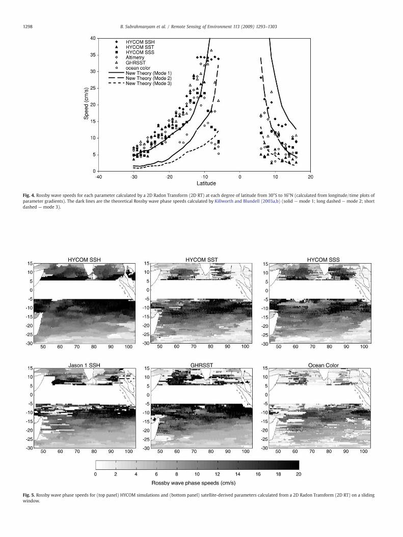
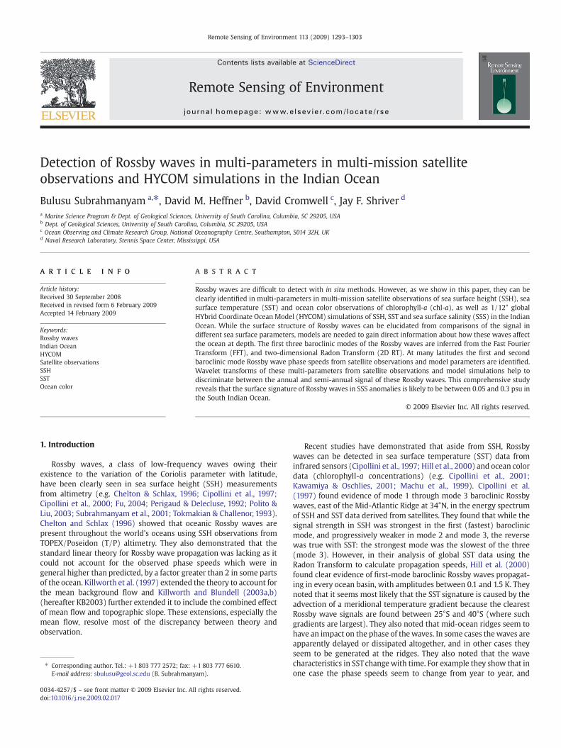
Fig. 4. Rossby wave speeds for each parameter calculated by a 2D Radon Transform (2D RT) at each degree of latitude from 30°S to 16°N (calculated from longitude/time plots ofparameter gradients). The dark lines are the theoretical Rossby wave phase speeds calculated by Killworth and Blundell (2003a,b) (solid — mode 1; long dashed — mode 2; shortdashed — mode 3).

Fig. 5. Rossby wave phase speeds for (top panel) HYCOM simulations and (bottom panel) satellite-derived parameters calculated from a 2D Radon Transform (2D RT) on a slidingwindow.

1298 B. Subrahmanyam et al. / Remote Sensing of Environment 113 (2009) 1293–1303

1299B. Subrahmanyam et al. / Remote Sensing of Environment 113 (2009) 1293–1303

4. Results and discussion

L/T plots along 10°S and 20°S of HYCOM simulations of SSH, SSTand SSS (Figs. 1 and 2 top panel) and satellite observations of Jason-1altimetry SSH, GHRSST and chl-a (Figs. 1 and 2 bottom panel) showclear propagation of Rossby waves from 2003–2006. In Fig. 1, theannual Rossby wave signal at 10°S can be clearly seen in HYCOM SSHand SSS, and Jason-1 altimetry. This signal is not as strong, but is stillvisible, in HYCOM SST, GHRSST, and ocean color chl-a. Also, with theexception of ocean color chl-a, all of the parameters appear to be inphase, where a propagating anomalous high in SSH, corresponds witha high in SST and SSS (this is true for both HYCOM and satellite-derived parameters). Ocean color chl-a however appears to be exactly180° out of phase, where a propagating high anomaly correspondswith a propagating anomalously low chl-a concentration.

In Fig. 2, a very strong Rossby wave-like signal at 20°S is present inHYCOM SSH and SSS, and a weaker signal is present in all the otherparameters. However, it is not clear from these diagrams whether it isan annual or semi-annual signal. The propagating SSH and SST anom-alies appear to be in phase at this latitude, however HYCOM SSS andsatellite-derived ocean color chl-a exhibit the opposite phase.

Thepower spectrumfromthe Fourier transformof eachparameterat10°S shows a strongpeakwitha period of about1 year, and awavelength

Fig. 6.Wavelet analysis of time series extracted from longitude/time plots of parameter anomimportant a certain wave period is at a given time). The bottom diagram is of the global wavdashed curve in the power spectrum figures is the cone of influence, below which edge effecglobal power diagrams is the 95% significance level (anything above is considered significant)ocean color (log of chl-a concentration).

in the 5500–8400 km range (Fig. 3 and Table 1). All of the parameterswith the exception of ocean color also show a peak with a period ofabout half a year and a wavelength around 2500 km. We believe thatthese correspond to the first and second-mode baroclinic Rossby wavescoincidingwith the theoretical values of Killworth and Blundell (2003a,b). There does appear to be some overlap in the speeds as shown inTable 1: 14.8–22.7 km/d for mode 1; and 12.2–15 km/d for mode 2. Thetheoretical speeds in this basin at 10°S are 25 km/d for mode 1 and13 km/d for mode 2. This discrepancy is possibly due to one or both ofthe following causes: 1) the truewavelength and periods of the featuresmay fall in-between two of the Fourier Transform bins, thus giving amuch larger range to the wavelengths and periods of the waves; 2) thesurface expression of the waves in ocean color chl-a and sea surfaceheight may be stronger in locations where the first-modewaves indeedhave a shorter wavelength.

Table 2 presents the amplitude of the surface expression of the first-mode baroclinic waves in each parameter as calculated from the Fouriertransform. The amplitudes in SSH and SST are comparable to the resultsreported by Quartly et al. (2003). Our calculated amplitude in HYCOMSSS of 0.03–0.3 psu suggests that the SMOS and Aquarius missionsshould be able to resolve Rossby waves in SSS at some latitudes.

The results of the Radon Transform (Fig. 4) for southern latitudescompare quite well with the new theoretical speed for Rossby waves

alies at 10°S 60°E. The top diagram of each subplot is thewavelet power spectrum (howelet power (how important a particular period is relative to the whole time series). Thets become important and results have to be treated with caution. The dashed line in the. A) HYCOM SSH, B) HYCOM SST, C) HYCOM SSS, D) Jason-1 altimetry, E) GHRSST, and F)

Fig. 7.Wavelet analysis of time series extracted from longitude/time plots of parameter anomalies at 10°S 90°E. The top diagram of each subplot is the wavelet power spectrum (howimportant a certain wave period is at a given time). The bottom diagram is of the global wavelet power (how important a particular period is relative to the whole time series). Thedashed curve in the power spectrum figures is the cone of influence below which edge effects become important and results have to be treated with caution. The dashed line in theglobal power diagrams is the 95% significance level (anything above is considered significant). A) HYCOM SSH, B) HYCOM SST, C) HYCOM SSS, D) Jason-1 altimetry, E) GHRSST, and F)ocean color (log of chl-a concentration).

1300 B. Subrahmanyam et al. / Remote Sensing of Environment 113 (2009) 1293–1303

given by Killworth and Blundell (2003a,b). Yet interestingly none of theparameters in the northern latitudes match the predicted first-modebaroclinic Rossby wave speeds. Heffner et al. (2008) proposed that thereason Radon Transform showed that the phase speed of the NorthernHemisphere Rossby waves did not match the predicted first-modeBaroclinic speeds was that we had treated the two basins as one ocean,instead of separating them. However, during the Radon Transformexercise for this study,we did indeed separate the two basins (figure notshown), and found that while HYCOM SSS at 10°N–18°N in the ArabianSea did track closer to firstmode, this was not true for other parameters.Additionally, none of the parameters in the Bay of Bengal tracked alongthe baroclinic first-mode speeds.

In Fig. 5 it can be seen that the 2DRTon a slidingwindowwasunableto resolve large portions of the Northern Hemisphere Rossby waves insatellite-derived parameters. HYCOM SST and SSS also appear quitenoisy, but all subplots seem to show a general trend that matches theHYCOM SSH speedmap. From the cleaner HYCOM SSHmap, we can seethat Rossby waves in the Northern Hemisphere indeed do appear totraverse more slowly than those features at comparable latitudes in theSouthern Hemisphere. And even more interesting is that in Fig. 4, if theNorthern HYCOM SSH phase speeds are shifted 5° to the North, theymatch the predicted Mode 1 phase speeds.

TheRossbywave speedmap (Fig. 5) shows a general pattern of fasterphase speeds toward theequator, gradating tomuch slower speeds in themid-latitudes (a 10° band centered around the equator has been blockedout). Interestingly there seems to be a sharper zonal gradient of thespeeds in the eastern part of the basin compared to the west. Thischange showsupclearest in theHYCOM(upperpart of Fig. 5) parameterswhere the band of speeds from 5–12 cm/s occupies a range from about18°S–15°S at 100°E, but this same band extends from 25°S–12°S by 50°E.The same trend can be seen in the satellite-derived parameters (lowerpart of Fig. 5), however there is somewhat more noise.

The results of the temporal wavelet transform (Figs. 6 and 7)clearly show a semi-annual and annual signal. These seem tocorrespond with the first and second baroclinic modes respectively,as pointed out in Fig. 3 and Table 1. It is interesting to note that thesemi-annual signal is rather strong in the western part of the basin,especially in HYCOM SSH and satellite-derived ocean color, where itspeak in the wavelet spectrum is comparable to the annual signal(Fig. 6). In the eastern part of the basin, the semi-annual signal israther weak with a small peak compared to the strong annual signal(Fig. 7). Also, interestingly with the exception of Jason-1 altimetry inthe west, all other parameters in both parts of the ocean have theirstrongest signals in July 2004 (∼1.5 years).

Fig. 8.Wavelet analysis of longitude series extracted from longitude/time plots of parameter anomalies at 20°S for July 15, 2004. The top diagram of each subplot is thewavelet powerspectrum (how important a certainwavelength is at a given time). The bottomdiagram is of the global wavelet power (how important a particular wavelength is relative to thewholetime series). The dashed curve in the power spectrum figures is the cone of influence, below which edge effects become important and results have to be treated with caution. Thedashed line in the global power diagrams is the 95% significance level (anything above is considered significant). A) HYCOM SSH, B) HYCOM SST, C) HYCOM SSS, D) Jason-1 altimetry,E) GHRSST, and F) ocean color (log of chl-a concentration).

1301B. Subrahmanyam et al. / Remote Sensing of Environment 113 (2009) 1293–1303

A wavelet analysis was also run in space to get an idea of how thewavelengths of the Rossby waves change while traversing the basin at20°S. (We also tried a spatial wavelet analysis at 10°S; however, at thislatitude the wavelengths of Rossby waves are too long to be resolved,and so fall under the cone of influence below which edge effectsbecome important. The cone of influence is defined formally as the e-folding time for the autocorrelation of wavelet power at each scale(Torrence & Compo, 1998). The spatial analysis was done at severaltimes (January 15, 2004 and 2005, and July 15, 2004 and 2005);however, only the July 2004 results are shown (Fig. 8). These timeswere chosen because: (1) they span the middle of the study period,and so most of the time series of the previous analyses at those timesfall above the cone of influence; and (2) the analyses presented inFigs. 6 and 7 (as well as other plots not shown) have strong peaks inthe energy plot at those times (not all parameters, however, hadstrong peaks at the same time).

It is important to note that there is a bathymetric feature called the90 East ridge in the Eastern Indian Ocean that spans about 50°S to15°N, running almost directly North–South, with a very slightEastward component. As the name implies, at its northern end it isnear the 90°E meridian (although at 20°S it runs almost parallel to the88°E meridian).

In July 2004 (Fig. 8), the HYCOM parameters all show a featurewith awavelength of about 2000 km to the east of the ridge that shiftssome energy into a shorter wavelength feature of about 800 km uponhitting the ridge and passing over it to the west. In ocean color chl-aand GHRSST, the 800 km feature appears on the east of the ridge anddissipates upon hitting it (this feature is barely visible in ocean colorchl-a largely due to an increasing trend to the east, which appears asthemassive N4100 kmwavelength signal in thewavelet analysis). This800 km feature also appears in Jason-1 altimetry and, like the HYCOMparameters (Fig. 9), it strengthens to the west of the ridge. However,instead of it “getting energy” from the 2000 km feature as it crossesthe ridge, it appears to provide energy to the longer wavelengthfeature at about 70°E, well to the west of the ridge.

5. Summary

Rossby waves are difficult to detect with in situ methods due toinsufficient space-time coverage. However, Rossby waves have thusfar been seen in several parameters derived from satellites such as seasurface height (SSH), sea surface temperature (SST) and ocean colorobservations of chlorophyll-a (chl-a). Up until this point, nobody hasshown that Rossby waves can be seen in global salinity field, largely

Fig. 9. (Top panel) HYCOM simulations of SST and SSS 4-year mean, and (bottom panel) meridional gradient of HYCOM SST and SSS 4-year mean.

1302 B. Subrahmanyam et al. / Remote Sensing of Environment 113 (2009) 1293–1303

because there is currently no easy way to acquire basin wide salinitydata. We did a preliminary study (Heffner et al., 2008) anddemonstrated that Rossby waves can be identified in the sea surfacesalinity (SSS) signal, using HYbrid Coordinate Ocean Model (HYCOM)simulations as a proxy for the awaited satellite-derived salinity data.

Observing Rossby wave signals in salinity will be helpful to betterunderstand these waves. While SST has a strong seasonal signal,salinity is only weakly affected by the changing seasons. It is alsoproblematic observing Rossby waves in ocean color because chlor-ophyll-a depends on various nutrient fields, which are not well knowncompared with standard physical oceanography fields such as(Evaporation–Precipitation) at the surface. A physical variable withbetter defined forcings, the variation of salinity should be much easierto understand than for a biological field.

While the structure of Rossby waves can be elucidated from com-parisons of the signal in different sea surface parameters, models areneeded to gain direct information about how these waves affectthe ocean at depth. The first three baroclinic modes of the Rossbywaves are inferred from the Fast Fourier Transform (FFT), and two-dimensional Radon Transform (2D RT). At many latitudes the first,second and third baroclinic mode Rossby wave phase speeds fromsatellite observations and model parameters are identified. Wavelettransforms of these multi-parameters from satellite observations andmodel simulations help to discriminate between the annual and semi-annual signal of these Rossby waves.

Future salinity missions, notably ESA's Soil Moisture and OceanSalinity (SMOS) and joint U.S. and Argentina Aquarius missions, willopen a new era in Rossby wave studies using high spatial and tem-poral coverage of satellite-derived salinity. HYCOM SSS range of 0.03–

0.3 psu demonstrates that these satellite missions should be able toresolve Rossby waves in SSS at some latitudes.

Acknowledgements

This work was supported in part by the NASA Physical Oceano-graphy Program under Grant NNG06GJ22G awarded to B.S. JS wassupported by the 6.1 project “Global and Remote Littoral Forcing inGlobal Ocean Models” sponsored by the Office of Naval Research(ONR) under program element 601153N. The HYCOM model resultswere obtained under grants of challenge and non-challengecomputer time from the Department of Defense High PerformanceComputing Program at the Naval Oceanographic Office, Stennis SpaceCenter, MS. We wish to give special thanks to Mr. Jeff R. Blundell forproviding helpful comments and discussion that greatly enhancedthis paper. We would also like to thank late Prof. Peter Killworth formaking the theoretical Rossby wave speed data available. Theauthors would like to thank two anonymous reviewers for theirvaluable comments and thorough review.

References

Challenor, P. G., Cipollini, P., & Cromwell, D. (2001). User of the 3D Radon Transform toexamine the properties of oceanic Rossby waves. Journal of Atmospheric and OceanicTechnology, 18, 1558−1566.

Charria, G., Dadou, I., Cipollini, P., Drévillon, M., De Mey, P., & Garçon, V. (2006).Understanding the influence of Rossbywaves on surface chlorophyll concentrationsin the North Atlantic Ocean. Journal of Marine Research, 64, 43−71.

Charria, G.,Mélin, F., Dadou, I., Radenac,M. -H.,&Garçon, V. (2003). Rossbywave andoceancolour: The cells uplifting hypothesis in the South Atlantic Subtropical ConvergenceZone. Geophysical Research Letters, 30, 1125. doi:10.1029/2002/GL016390.

1303B. Subrahmanyam et al. / Remote Sensing of Environment 113 (2009) 1293–1303

Chelton, D. B., & Schlax, M. G. (1996). Global observations of oceanic Rossby waves.Science, 272, 234−238.

Cipollini, P., Cromwell, D., Challenor, P. G., & Raffaglio, S. (2001). Rossby waves detectedin global ocean colour data. Geophysical Research Letters, 28, 323−326.

Cipollini, P., Cromwell, D., Jones, M. S., Quartly, G. D., & Challenor, P. G. (1997). Concur-rent altimeter and infrared observations of Rossby wave propagation near 34°N inthe Northeast Atlantic. Geophysical Research Letters, 24, 889−892.

Cipollini, P., Cromwell, D., Quartly, G. D., & Challenor, P. G. (2000). Remote sensing ofoceanic extra-tropical Rossby waves. In David Halpern (Ed.), Satellites, oceano-graphy, and society (pp. 99−123). New York: Elsevier.

Cromwell, D. (2001). Sea surface height observations of the 34°N ‘waveguide’ in theNorth Atlantic. Geophysical Research Letters, 19, 3705−3708.

Dandonneau, Y., Vega, A., Loisel,H., du Penhoat, Y., &Menkes, C. (2003).OceanicRossbywavesacting as a “hay rake” for ecosystem floating by-products. Science, 302, 1548−1551.

Deans, S. R. (1983). The Radon Transform and some of its applications. New York: JohnWiley.

Foufoula-Georgiou, E., & Kumar, P. (1994). Wavelets in Geophysics. San Diego: AcademicPress.

Fu, L. L. (2004). Latitudinal and frequency characteristics of the westward propagationof large-scale oceanic variability. Journal of Physical Oceanography, 34, 1907−1921.

Graps, A. (1995). An introduction to wavelets. IEEE Computational Science & Engineering,2, 50−61.

Heffner, D. M., Subrahmanyam, B., & Shriver, J. F. (2008). Indian Ocean Rossby wavesdetected in HYCOM sea surface salinity. Geophysical Research Letters, 35, L03605.doi:10.1029/2007GL032760.

Hill, K. L., Robinson, I. S., & Cipollini, P. (2000). Propagation characteristics of extra-tropical planetary waves observed in the ASTR global sea surface temperaturerecord. Journal of Geophysics Research, 105, 21927−21945.

Kawamiya, M., & Oschlies, A. (2001). Formation of a basin-scale surface chlorophyllpattern of Rossby waves. Geophysical Research Letters, 28, 4139−4142.

Kerr, Y., Font, J., Waldteufel, P., & Berger, M. (2000). The second of ESA's opportunitymissions: The Soil Moisture and Ocean Salinity Mission — SMOS. ESA Earth Observ-ation Quarterly, 66, 18f.

Killworth, P. D., & Blundell, J. R. (2003). Long extratropical planetary wave propagationin the presence of slowly varying mean flow and bottom topography. Part I: Thelocal problem. Journal of Physical Oceanography, 33, 784−801.

Killworth, P. D., & Blundell, J. R. (2003). Long extratropical planetary wave propagationin the presence of slowly varying mean flow and bottom topography. Part II: Ray

propagation and comparison with observations. Journal of Physical Oceanography,33, 802−821.

Killworth, P. D., Chelton, D. B., & de Szoeke, R. (1997). The speed of observed andtheoretical long extratropical planetary waves. Journal of Physical Oceanography, 27,1946−1966.

Killworth, P. D., Cipollini, P., Uz, B. M., & Blundell, J. R. (2004). Physical and biologicalmechanisms for planetary waves observed in satellite-derived chlorophyll. Journalof Geophysics Research, 109, C07002. doi:10.1029/2003JC001768.

Lagerloef, G. S. E. (2001). Satellite measurements of salinity. In J. Steele, S. Thorpe, & K.Turekian (Eds.), Encyclopedia of Ocean Sciences (pp. 2511−2516). London: AcademicPress.

Machu, E., Ferret, B., & Garçon, V. (1999). Phytoplankton pigment distribution fromSeaWiFS data in the subtropical convergence zone south of Africa: A waveletanalysis. Geophysical Research Letters, 26, 1469−1472.

Maritorena, S., Siegel, D.A., Hembise Fanton d'Andon, O., Mangin, A. (submitted forpublication). Ocean Color Merged Data Sets: Benefits and Challenges. Remote Sens.of Envi.

Meyers, S. D., Kelly, B. G., & O'Brien, J. J. (1993). An introduction to wavelet analysis inoceanography and meteorology: With application to the dispersion of Yanai waves.Monthly Weather Review, 121, 2858−2866.

Perigaud, C., & Delecluse, P. (1992). Annual sea level variations in the southern tropicalIndian Ocean from Geosat and shallow-water simulations. Journal of GeophysicsResearch, 97, 20169−20178.

Polito, P. S., & Liu, W. T. (2003). Global characterization of Rossby waves at several spectralbands. Journal of Geophysics Research, 108, C13018. doi:10.1029/2000JC0000607.

Quartly, G.D., Cipollini, P., Cromwell, D., & Challenor, P. G. (2003). Rossbywaves: Synergy inaction. Philosophical Transactions of the Royal Society of London. A, 361, 57−63.

Siegel, D. A. (2001). The Rossby rototiller. Nature, 409, 576−577.Subrahmanyam, B., Robinson, I. S., Blundell, J. R., & Challenor, P. G. (2001). Indian Ocean

Rossby waves observed in TOPEX/POSEIDON altimeter data and in modelsimulations. International Journal of Remote Sensing, 22, 141−167.

Tokmakian, R. T., & Challenor, P. G. (1993). Observations in the Canary Basin and the AzoresFrontal region using Geosat data. Journal of Geophysics Research, 98, 4761−4773.

Torrence, C., & Compo, G. P. (1998). A practical guide to wavelet analysis. Bulletin of theAmerican Meteorological Society, 79, 61−78.

Uz, B. M., Yoder, J. A., & Osychny, V. (2001). Pumping of nutrients to ocean surfacewaters by the action of propagating planetary waves. Nature, 409, 597−600.