Mechanisms Setting the Strength of Orographic Rossby Waves ...

Mechanisms Setting the Strength of Orographic Rossby Wavesacross a Wide Range of Climates in a Moist Idealized GCM

ROBERT C. J. WILLS

University of Washington, Seattle, Washington

TAPIO SCHNEIDER

California Institute of Technology, Pasadena, California

(Manuscript received 21 October 2017, in final form 30 May 2018)

ABSTRACT

Orographic stationary Rossby waves are an important influence on the large-scale circulation of the at-

mosphere, especially in Northern Hemisphere winter. Changes in stationary waves with global warming have

the potential to modify patterns of surface temperature and precipitation. This paper presents an analysis of

the forcing of stationary waves by midlatitude orography across a wide range of climates in a moist idealized

GCM, where latent heating and transient eddies are allowed to feed back on the stationary-eddy dynamics.

The stationary-eddy amplitude depends to leading order on the surface winds impinging on the orography,

resulting in different climate change responses for mountains at different latitudes. Latent heating is found to

damp orographic stationary waves, whereas transient eddies are found to reinforce them. As the climate

warms, the damping by latent heating becomes more effective while the reinforcement by transient eddies

becomes less effective, leading to an overall reduction in orographic stationary wave amplitude. These effects

overwhelm the influences of a reduced meridional temperature gradient and increased dry static stability,

both of which increase the sensitivity of the free troposphere to orographic forcing. Together with a reduction

in the midlatitude meridional temperature gradient, the weakening of orographic stationary waves leads to

reduced zonal asymmetry of temperature and net precipitation in warm, moist climates. While circulation

changes in this idealized model cannot be expected to agree quantitatively with changes in the real world, the

key physical processes identified are broadly relevant.

1. Introduction

Large-scale orography such as the Tibetan Plateau,

Rocky Mountains, and Andes influence the general

circulation of the atmosphere by exciting planetary-

scale stationary Rossby waves (Hoskins and Karoly

1981; Held et al. 2002) with consequences for the

zonal variation of temperature (Lau 1979; Kaspi and

Schneider 2011; Deser et al. 2014; Hoskins and

Woollings 2015) and precipitation (Peixóto and Oort

1983, 1992; Broccoli and Manabe 1992; Wills and

Schneider 2015, 2016). Orographic Rossby waves are

particularly important for the dryness of central

North America and Asia in winter (Broccoli and

Manabe 1992), the maintenance of summertime sub-

tropical circulation patterns (Rodwell and Hoskins

2001), and the seasonality and strength of precipitation

in the East Asian monsoon region (Molnar et al. 2010;

Chen and Bordoni 2014). The response of these re-

gional climate features to global warming will thus de-

pend on the response of orographic Rossby waves.

Some studies have suggested that the strength of oro-

graphic stationary waves should increase with global

warming as a result of the decreased lower-tropospheric

meridional temperature gradient (Cook and Held 1988;

Held 1993), but this is only one influence out of many on

the amplitude of stationary waves.

Coupled climate models can give predictions of the

stationary wave response to climate change over the

next century (Stephenson and Held 1993; Joseph et al.

2004; Vecchi and Soden 2007; Brandefelt and Körnich2008; Wang and Kushner 2011; Simpson et al. 2014,

2016). However, the stationary wave response in these

models is a superposition of the response to several

different stationary wave sources, complicating an as-

sessment of the dominant physical mechanisms forCorresponding author: Robert C. Jnglin Wills, [email protected]

15 SEPTEMBER 2018 W I L L S AND SCHNE IDER 7679

DOI: 10.1175/JCLI-D-17-0700.1

� 2018 American Meteorological Society. For information regarding reuse of this content and general copyright information, consult the AMS CopyrightPolicy (www.ametsoc.org/PUBSReuseLicenses).

mailto:[email protected]

http://www.ametsoc.org/PUBSReuseLicenses



these changes. Traditionally, stationary waves have

been split into components attributed to different

forcings using stationary wave models: general circu-

lation models in which transient eddies are strongly

damped (Ting and Yu 1998; Held et al. 2002) or that

explicitly solve the linearized primitive equations

(Egger 1976; Hoskins and Karoly 1981; Nigam et al.

1986, 1988; Valdes and Hoskins 1989; Ting 1994). The

climatology and climate change response of station-

ary waves are well simulated by such models (Nigam

et al. 1988; Stephenson and Held 1993), but they rely

on specifying diagnosed diabatic tendencies, which

themselves depend on the stationary wave solution.

Stephenson and Held (1993) find that changes in la-

tent heating and transient-eddy heat and momentum

fluxes, rather than changes in the zonal-mean basic

state, dominate the stationary wave response to global

warming. This highlights the importance of under-

standing moist processes and transient eddies as they

change with global warming. In the modern climate,

much of the zonal asymmetry in latent heating and

transient-eddy heating is either directly or indirectly a

response to orography (Nigam et al. 1988). Thus, in or-

der to study changes in diabatic tendencies associated

with orography and their role in modifying orographic

stationary Rossby waves under climate change, we use a

moist general circulationmodel (GCM), where transient

eddies are simulated explicitly and latent heating is al-

lowed to feed back on the dynamics.

In Wills and Schneider (2016, hereinafter WS16), we

present idealized GCM experiments in which individual

topographic and ocean-heating zonal asymmetries are

added to an aquaplanet. This allows an analysis of the dif-

fering responses to climate change of stationary waves

forced by these two types of zonally asymmetric forcings.

We simulate a wide range of climates from cold, dry cli-

mates (280-K global-mean surface temperature), where the

influence of latent heating is negligible, to warm, moist cli-

mates (nearly 320-K global-mean surface temperature),

where latent heating plays a leading-order role inmodifying

stationary-eddy circulations. The response of stationary-

eddy vertical velocity to warming is characterized by a

strong decrease with warming when stationary eddies

are forced by equatorial heating, and by a nonmonotonic

response to warming when stationary eddies are forced

by midlatitude orography (WS16). The vertical velocity

response, which is important for changes in precipitation

minus evaporation, mirrors changes in the horizontal

flow as a result of the linear vorticity balance in the lower

troposphere (WS16). In Wills et al. (2017), we study the

mechanisms responsible for the zonally asymmetric

circulation changes in the equatorial heating experi-

ment. Here, we focus on the mechanisms responsible for

changes in the strength of stationary waves in the mid-

latitude orographic forcing experiment.

There is an expectation from quasi-geostrophic

theory that the strength of orographic stationary

waves should depend on the strength of the mean low-

level winds at the latitude of the mountain (Hoskins

and Karoly 1981; Held 1983; Held and Ting 1990). The

role of the low-level winds arises from their role in

setting the strength of topographic vertical motions,

which influence the atmosphere through adiabatic

cooling or heating. Nonlinear modification of the to-

pographic vertical motions by the stationary wave

response reduces the strength of the adiabatic cooling

and heating tendencies (Chen and Trenberth 1988;

Valdes and Hoskins 1991; Ringler and Cook 1997),

but it does not change the conclusion that these adia-

batic tendencies are the primary way in which orogra-

phy influences the free troposphere. In the midlatitudes,

this adiabatic cooling/heating can be balanced by me-

ridional advection along the large meridional temper-

ature gradient. This meridional flow perturbation sets

up a stationary Rossby wave with eastward group ve-

locity (Hoskins and Karoly 1981). The meridional wind

response can be modified by additional heating ten-

dencies, such as the latent heating associated with

orographic vertical motion or the transient-eddy heat

fluxes associated with initiation of a storm track down-

stream. We can analyze the mechanisms governing

changes in the strength of the resulting stationary

Rossby wave using an analysis of the thermodynamic

equation over the orography (cf. Hoskins and Karoly

1981). This is effectively an analysis of the boundary

condition for quasi-geostrophic theory, which is the

only way in which topography explicitly enters the

quasi-geostrophic equations (Hoskins and Karoly 1981;

Vallis 2006).

Considering the importance of the low-level wind

and the meridional temperature gradient (both of

which vary strongly with latitude) for the orographic

forcing of stationary waves, we expect the stationary

wave response to climate change will depend on the

latitude of orographic forcing. We therefore run sim-

ulations with topography at different latitudes, de-

scribed in section 2. The stationary wave response to

climate change forced by increased greenhouse gas

absorption is described in section 3. In section 4, we

analyze the forcing of upslope and downslope oro-

graphic winds by surface flow over and around to-

pography. In section 5, we analyze the thermodynamic

equation over the orography to understand the mecha-

nisms through which the atmosphere responds to

the orographic vertical winds and determine the fac-

tors important in the climate change response. In

7680 JOURNAL OF CL IMATE VOLUME 31

section 6, we discuss how the stationary wave changes

lead to a reduction in the midlatitude zonal variance

of temperature and precipitation in the warmest cli-

mates studied. Section 7 summarizes the paper and

presents our conclusions, and section 8 discusses the

implications of our results for the real world.

2. Idealized GCM experiments

To isolate the response of orographically forced

stationary Rossby waves to global warming, we add

a single large-scale mountain ridge to an idealized

GCM simulation with otherwise zonally symmetric

aquaplanet boundary conditions. These simulations

are described in WS16, which focuses on the response

of the zonally asymmetric hydrological cycle to global

warming. The model used is that of Frierson et al.

(2006) and O’Gorman and Schneider (2008b), based

on the GFDL Flexible Modeling System and the con-

vection scheme of Frierson (2007). The model is run at

T85 spectral resolution, with 38 levels in the vertical.

There is a sponge layer in the top eight model levels

in order to avoid reflections of planetary waves from

the top of the domain, as described in WS16. Our

simulations use a 1-m slab oceanmixed layer depth and

a specified zonally symmetric ocean heat flux conver-

gence that does not extend into latitudes where to-

pography is present (see WS16).

The surface topography is specified as a function of

longitude l and latitude f by

zs(l,f)5 h

0exp

2642(l2 l

0)2

2s2l

2max(0, jf2f

0j2R

f)2

2s2f

375,(1)

where we use h0 5 2500m, Rf 5 2.58, sf 5 58, andsl 5 12.58. We use two different orographic configu-

rations, f0 5 458 and 548N, which we refer to as R45

and R54, respectively. The profile of the topography in

each experiment is shown inFig. 1. TheR45 experiment is

set up to be qualitatively similar to the orographic forcing

by the combined Rocky Mountains, Sierra Nevada, and

Pacific Northwest Coastal Ranges and is the experiment

studied in WS16. The R54 experiment is set up such that

the latitude of the mountain coincides with the latitude of

maximum change in zonal surface westerlies across the

range of climates.

FIG. 1. (a) Barotropic streamfunction and (b) zonally anomalous lower-tropospheric (550–750 hPa) meridional

wind forced by orography in the reference simulation (a5 1, global-mean surface temperature Tg 5 289K) and in

the 3 times optical depth simulation (a5 3,Tg5 307K) for bothmountain configurations (R45 andR54). The black

contours show the 800- and 900-hPa contours of surface pressure.


To focus exclusively on the atmospheric response to

orography, we keep the surface properties over to-

pography the same as in the surrounding aquaplanet

(i.e., the mountains are aquamountains). Note also that

the idealized GCM does not consider the liquid–solid

phase change, so there is no atmospheric ice conden-

sate or sea ice over the elevated topography. The sur-

face of the mountain differs from a land surface by its

higher heat capacity, lower albedo, and lack of water

limitation. The philosophy of this decision is that any

modification of the surface boundary condition (e.g.,

albedo) would provide an additional source of sta-

tionary waves, with different physics, that should be

studied separately.

We have investigated zonal mountain scales sl

ranging from 28 to 508 longitude (Wills 2016). The

stationary wave amplitude is maximum at sl’ 158. We

chose sl 5 12.58 to force a large-amplitude Rossby

wave while keeping the mountain size realistic. For

narrower mountains, the response is confined to the

local orographic precipitation influence (cf. Shi and

Durran 2014). At T85 resolution, there starts to be

substantial grid-scale noise for sl # 58. Such resolution

issues are likely the cause of grid-scale noise in IPCC

models (cf. Wills et al. 2016).

Global warming is simulated by rescaling the long-

wave optical depth t5atref by a factor a, where tref is a

reference optical depth that is a function of latitude and

pressure (O’Gorman and Schneider 2008b):

tref

(f, ~p)5 [ fl~p1 (12 f

l)~p4][te 1 (tp 2 te) sin

2 f] . (2)

Here, fl 5 0:2, ~p is pressure expressed in nondimensional

standard atmospheres, and the longwave optical thick-

ness at the equator and at the pole are te 5 7:2 and

tp 5 3:6, respectively. Note that while the model uses

sigma coordinates, the optical depth is specified as a

function of pressure such that the atmospheric column is

optically thinner over elevated topography. The optical

depth in this model is not modified by water vapor or

cloud radiative feedbacks and is thus fixed throughout

each simulation. These simulations are ‘‘moist’’ princi-

pally because latent heating is allowed to feed back on the

dynamics. We use 16 values of the rescaling factor

a5 [0.6, 0.7, 0.8, 0.9, 1.0, 1.2, 1.4, 1.6, 1.8, 2.0, 2.5, 3.0, 4.0,

6.0], such that we simulate climates with global-mean

surface temperatures ranging from 280 to 316K. Each

simulation is spun up for nine years and averaged over the

following eight years.

3. Stationary wave response

In each simulation, the time-mean barotropic stream-

function (Fig. 1a) or zonally anomalous meridional winds

(Fig. 1b) shows a stationary Rossby wave emanating from

the topography, with a wave train extending southeast

into the tropics. The zonal wavenumber of the stationary

wave is predominantly a mix of wavenumbers 1–4 and

does not show a large change with warming. While

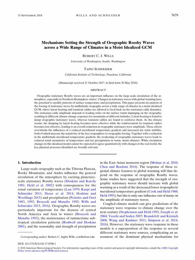
FIG. 2. Vertical profile of sEKE [Eq. (3)] superimposed on contours of the zonal-mean zonal wind (contour interval 5m s21, thick

contour is the [u]5 0 line). (left)–(right) Three climates (a 5 0.8, 1.6, and 4.0) are shown for both the (top) R45 and (bottom) R54

experiments. Temperatures in parenthesis show the global-mean surface temperature. Also shown is the tropopause height computed

from the 2K km21 lapse-rate criterion (blue line). The filled triangle in each plot shows the latitude of the topographic peak f0.


length scale changes resulting from strengthening

of the upper-tropospheric jet stream have been im-

plicated in the stationary wave response to climate

change over the next century (Simpson et al. 2016),

the length scale of the stationary waves is too large for

this to be an important mechanism in our simulations,

since it is important primarily for zonal wavenumbers

k . 4. Length scale changes may be an important

factor in the climate response of stationary waves

forced by orography with a smaller zonal scale.

The stationary wave ray paths (i.e., the southeast-

ward trajectory of the wave train into the tropics) can

be understood in terms of ray-tracing theory (Hoskins

and Karoly 1981) and depend on the structure of the

zonal-mean winds. The zonal-mean winds in the ide-

alized GCM (contours in Fig. 2) are not particularly

realistic; they lack a distinct upper-tropospheric

maximum and show an equatorward shift of the

surface westerlies with climate change. Therefore,

investigation of the precise ray paths and spatial

structure of the stationary Rossby waves in this model

would not necessarily lead to insights about station-

ary wave changes in the real world. Instead, we focus

on the mechanisms controlling the strength of sta-

tionary waves, which should translate to more re-

alistic settings.

We measure the strength of stationary Rossby waves

by the stationary-eddy kinetic energy,

sEKE[1

2r(u*2 1 y*2) , (3)

a bulk measure of the stationary-eddy wind strength.

Here, u is the zonal wind, y is the meridional wind, and

r is the time- and zonal-mean density. Stationary eddies

are characterized by time-mean deviations from the

zonal mean,

(�)*[ (�)2 [�] , (4)

where time averages are denoted by (�) and zonal av-

erages are denoted by [�].Stationary-eddy kinetic energy is distributed through-

out the troposphere and lower stratosphere in the

hemisphere of forcing (Fig. 2). The sEKE is high in

the lower troposphere at the latitude of forcing, then

grows with height following the direction of vertical

and meridional propagation to a local maximum in

the upper troposphere near the latitude of maximum

zonal wind. The upper-tropospheric maximum re-

flects the refraction of Rossby waves into the jet

stream (Hoskins and Karoly 1981). Note that the

latitude–pressure profile of zonal-mean zonal wind

does not differ significantly between R45 and R54

and can thus be thought of as independent of the

latitude of topographic forcing. In most of the simu-

lations shown here, a weaker secondary wave train

can be seen propagating poleward from the mountain,

consistent with ray-tracing theory (Hoskins and

Karoly 1981).

The planetary waves studied here propagate vertically

within the troposphere; all but the longest waves are

evanescent beyond the tropopause. The vertical struc-

ture of sEKE within the troposphere is therefore de-

termined largely by the stationary external mode

(Held et al. 1985). The vertical dispersion of stationary

Rossby waves is inhibited in warm climates because of

the increased upper-tropospheric vertical winds (cf.

Charney and Drazin 1961), which results from the

stronger warming of the tropical upper troposphere

relative to the extratropical upper troposphere–lower

stratosphere. This primarily affects the distribution

of sEKE in the stratosphere and upper troposphere

(compare in particular the decay of sEKE above

500 hPa for a 5 1.6 and 4.0 in Fig. 2). This trap-

ping of stationary waves in the lower troposphere

may contribute to the reduction of sEKE in the

warmest climates. It can equivalently be thought of

as a consequence of the contrasting responses of the

FIG. 3. Variation of global-mean vertically integrated sEKEwith

global warming in the (a) R45 and (b) R54 experiments. The sEKE

is vertically integrated over the full column. Filled symbols indicate

the reference climate (a 5 1).


upper- and lower-tropospheric meridional tempera-

ture gradients, since the meridional temperature gra-

dient sets the strength of stationary-eddy meridional

wind required to balance a given heat source, as will be

discussed in section 5.

To average over any particular differences in sta-

tionary wave ray paths between simulations and focus

on the global changes in the strength of stationary

waves, we compute the global-mean vertically inte-

grated sEKE. This measure still incorporates informa-

tion about changes in the zonal, meridional, and height

extent of stationary wave activity, which can arise be-

cause of changes in meridional and vertical dispersion,

but it allows easy comparison between simulations with

different stationary wave ray paths. There is an increase

in global sEKE with warming in the R45 experiment

until a global-mean surface temperature of 300K (a5 1.8)

is reached, at which point there is a pronounced re-

duction in sEKE with further warming (Fig. 3a). In

contrast, the R54 experiment shows a monotonic re-

duction of global sEKE throughout the range of climates

(Fig. 3b).

The main goal of this paper is to provide physical

mechanisms for the response of the stationary wave

amplitude to warming in these simulations. In particu-

lar, we hope to explain the reasons for the reduction

of sEKE in the warmest climates and the differences in

sEKE for mountains at different latitudes. While

sEKE is just one possible measure of stationary wave

amplitude, we have found that other measures (e.g.,

variance of barotropic streamfunction and wave ac-

tivity) agree with the sense of change in stationary

wave amplitude as diagnosed from sEKE. In most of

what follows, we focus on the sEKE contribution from

the meridional wind variance y*2, which shows similar

fractional changes to the total sEKE across the range

of climates.

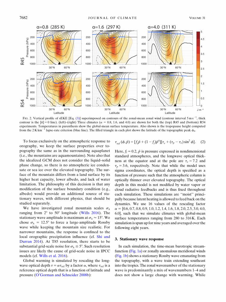
4. Mechanical forcing by orography

The principal means by which the atmosphere

‘‘feels’’ orography is through the mechanical com-

pression of the atmospheric column. This results in

net upward motion on the windward side of a

mountain and net subsidence in the lee (Fig. 4a).

The strength of the orographic vertical pressure

velocity vsfc, in a long-term average, is set at the

surface by the horizontal surface winds usfc and

the horizontal gradient of surface pressure =ps over

topography:

vsfc

5 usfc

� =ps. (5)

Before we discuss the thermodynamics of the response

to this perturbation in the next section, it is useful to

discuss the controls on vsfc, because these factors help to

explain stationary wave amplitude differences between

the R45 and R54 experiments.

In the midlatitudes, the zonal-mean westerlies by

themselves would lead to large orographic vertical

velocities according to [usfc]›xps, leading to ascent on

the western side of the mountain and descent on the

eastern side (Fig. 4b). However, the stationary-eddy

surface wind response reduces the strength of ascent/

descent as a result of the tendency of the cli-

matological wind to follow surface pressure contours

FIG. 4. (a) Map of vsfc* over topography (shading) in the reference climate of R45. Also shown are the horizontal

surface winds (usfc, vectors) and two contours (900 and 800 hPa) of surface pressure (black contours). (b)–(d)

Components of vsfc* based on the decomposition in Eq. (6) and the corresponding surface wind vectors.


around the mountain. This results in an opposing

contribution to the orographic vertical velocity of the

form usfc* � =ps*(Fig. 4c). This effect has been shown to

reduce the amplitude of orographic stationary waves

compared to linear models (Chen and Trenberth

1988; Valdes and Hoskins 1991; Ringler and Cook

1997) and leads to a sublinear dependence of oro-

graphic stationary wave amplitude on topographic

height (Lutsko and Held 2016; Wills 2016). The full

orographic vertical velocity can be expressed in terms

of the components attributed to the zonal-mean and

stationary-eddy surface winds according to

vsfc* ’ ([u

sfc]1 u

sfc* ) � =p

s*1 y

sfc* ›

y[p

s] . (6)

The last term on the right-hand side of Eq. (6) is negli-

gible because j=ps*j � j›y[ps]j. The full zonal-meanwind

term [usfc] � =ps* (Fig. 4d), including the zonal-mean

meridional surface winds, is the same magnitude as the

zonal-mean zonal wind term (Fig. 4b), but the upslope

vertical winds are shifted slightly to the southwest by the

zonal-mean southerly winds in the midlatitudes.1

Although the zonal-mean zonal wind term, [usfc]›xps

is a factor of 2 larger than vsfc* , one might expect them to

scale similarly with warming. Basically, this is assuming

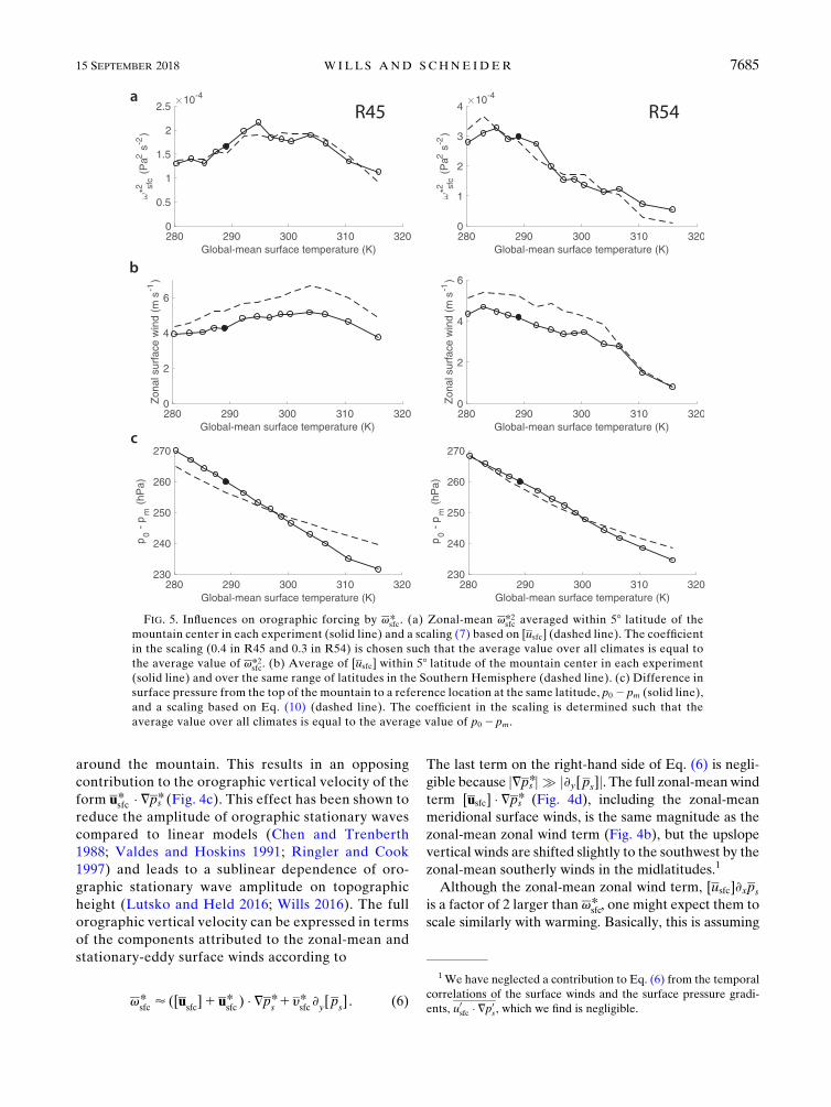
FIG. 5. Influences on orographic forcing by vsfc* . (a) Zonal-mean vsfc*2 averaged within 58 latitude of the

mountain center in each experiment (solid line) and a scaling (7) based on [usfc] (dashed line). The coefficient

in the scaling (0.4 in R45 and 0.3 in R54) is chosen such that the average value over all climates is equal to

the average value of vsfc*2. (b) Average of [usfc] within 58 latitude of the mountain center in each experiment

(solid line) and over the same range of latitudes in the Southern Hemisphere (dashed line). (c) Difference in

surface pressure from the top of the mountain to a reference location at the same latitude, p0 2 pm (solid line),

and a scaling based on Eq. (10) (dashed line). The coefficient in the scaling is determined such that the

average value over all climates is equal to the average value of p0 2pm.

1We have neglected a contribution to Eq. (6) from the temporal

correlations of the surface winds and the surface pressure gradi-

ents, u0sfc � =p0

s, which we find is negligible.


that the flow is deflected around topography to the same

extent in all simulated climates. In this case, the oro-

graphic vertical velocity variance would scale with the

zonal-mean zonal wind according to

d[vsfc* ]; d[[u

sfc]2(›

xps*)

2] . (7)

We find that this scaling describes well the changes in

vsfc*2 with warming in both experiments (Fig. 5a), ex-

cept in the warmest two climates of the R54 experi-

ment, where [usfc] at the latitude of the mountain is

small. The constant of proportionality relating the

left- and right-hand sides of Eq. (7) is 0.4 in R45 and

0.3 in R54, indicating that the stationary-eddy surface

winds reduce the strength of mechanical orographic

forcing by approximately 60%–70% (cf. Chen and

Trenberth 1988; Valdes and Hoskins 1991; Ringler

and Cook 1997).

Based on this scaling, the topographic vertical ve-

locity reflects the zonal-mean zonal surface wind at

the latitude of the mountain (Fig. 5b), which has a

different warming response at different latitudes be-

cause of the equatorward shift of the surface west-

erlies with warming in the idealized GCM (Fig. 6). In

these simulations, the 548N mountain sees a mono-

tonic decrease in the zonal-mean westerlies and the

458N mountain sees a nonmonotonic change in the

zonal-mean westerlies, responses that are reflected in the

orographic vertical velocity changes. The equatorward

shift of the zonal surface winds with warming mirrors the

equatorward shift of upper-tropospheric transient-eddy

kinetic energy (tEKE) in this idealized GCM (Wills

2016). This is in contrast to lower-tropospheric tEKE,

which shifts poleward with warming, as seen also in ob-

servations and comprehensive climatemodels (Fyfe 2003;

Yin 2005; Bender et al. 2012; Chang et al. 2012). The

opposite direction of response in surface winds

compared to observations and comprehensive models

stems from the unrealistic structure of the upper-level

winds in this gray-radiation idealized GCM and

can be corrected by improving the representation

of radiation (Z. Tan, 2017 personal communica-

tion). This paper aims to understand the mechanisms

controlling the amplitude of orographic stationary

waves as a function of mean climate state, rather

than the climate response for a particular mountain

range and mean climate state, so the equatorward

shift of the zonal westerlies does not pose a serious

problem here.

In addition to the effect of zonal surface wind

changes, there is a small reduction in vsfc*2 with warm-

ing due to the reduction of topographic pressure gra-

dients ›xps* (Fig. 5c), which contribute to the scaling

(7). The pressure gradient can be expressed in terms of

the difference in time-mean surface pressure between

the top of the mountain pm and a reference point at sea

level p0,

[(›xps*)

2]’ (p

m2p

0)2/p2r2e cos

2 f , (8)

where re is the radius of Earth.2 The change is dominated

by an increase in pm, which weakens the orographic

forcing of stationary waves in warmer climates by

approximately 10% compared to the reference cli-

mate. Since =ps*also shows up in the nonlinear term of

Eq. (6), the influence of pm on the total orographic

forcing should remain, no matter the structure of the

surface winds.

The increase in top-of-mountain pressure pm is a

simple thermodynamic consequence of the warming

of the lower troposphere. Using hydrostatic balance,

›z lnp52g/RT, we may obtain an expression for the

pressure at height zm (the height of the mountain) over

a point where the surface pressure is p0 by integrating

vertically from the surface:

ln p(zm)’ ln p

02

ðzm0

g

RTdz . (9)

Here, R is the specific gas constant of dry air. Assuming

that time-mean horizontal pressure differences at zm(normally of order 10 hPa) are much less than p0 2pm ;250 hPa, then p(zm)’ pm. Substituting an approxi-

mate temperature profileT(z)5T0 2G0z, we obtain an

FIG. 6. Variation of zonal-mean zonal surface wind [usfc] with

warming across the range of climates. Zonal averages are shown

for the Southern Hemisphere such that values are equivalent

for R45 and R54. Northern Hemisphere winds are up to about

1m s21 weaker because of the presence of topography (Fig. 5b).

Dashed lines indicate the latitude of the mountain center in each

experiment.

2While the mountain length scale sl would show up in a scaling

for the local ›xps*, the relevant length scale for the zonal-mean zonal

pressure gradient variance [(›xps*)2] is precosf.


expression for the top-of-mountain pressure in terms

of a reference lapse rate G0 and a reference surface

temperature T0,

pm’ p

0

�12

G0zm

T0

�g/RG0

. (10)

Evaluating T0 as an average surface temperature at

the latitude of the mountain in the eastern hemisphere

(away from the mountain) and G0 as an average

lapse rate over the bottom 250 hPa of the troposphere

in the same region, we obtain the approximate p0 2 pm

shown as a dashed line in Fig. 5c. By fixing T0 and G0

independently (not shown), we can see that the in-

crease in top-of-mountain pressure is a direct con-

sequence of changes in surface temperature T0;

the influence of changes in G0 is negligible for

the range of climates studied here. This thermody-

namic increase in top-of-mountain pressure has al-

ready been observed over the past century (Toumi

et al. 1999).

The orographic vertical winds, which set the initial

orographic perturbation to the atmosphere, are sen-

sitive to changes in the zonal-mean zonal surface

winds, in the top-of-mountain surface pressure, and in

the stationary-eddy modification of surface winds.

When the orography lies fully within the surface

westerlies, the changes are determined largely by

changes in the strength of the zonal-mean zonal sur-

face winds. There is an additional tendency toward

weaker forcing in warmer climates as the top-of-

mountain surface pressure increases with warming.

The orographic vertical velocity variance vsfc*2 is the

simplest measure that gives a qualitative sense of the

strength of orographic forcing of stationary waves

and the response of stationary wave amplitude (i.e.,

sEKE) to climate change in our simulations. In the

next section, we will examine how the atmosphere

responds to this mechanical surface forcing. It is

worth noting that we designed the R54 experiment to

get the maximum zonal surface wind response to

climate change at the latitude of the mountain, with

the hypothesis that as the zonal winds go to zero at

this latitude, the stationary wave response would be

dramatically reduced. This hypothesis was verified by

these simulations.

5. Thermodynamic response to orographic forcing

To understand how the atmosphere responds to oro-

graphic vertical winds, we study the thermodynamic

tendencies that balance the lower-tropospheric adia-

batic cooling and heating induced by the orographic

vertical winds.We examine the zonally anomalous steady-

state thermodynamic balance,

(u›xu*1 y›

yu1v›pu)*1=

r� (v0u0)*5Q* . (11)

Here,v is the vertical pressure velocity, u is the potential

temperature, and

Q*5Qlatent* 1Q

radiation* 1Q

sub-grid* (12)

is the zonally anomalous heating tendency by latent

heating, radiation, and subgrid-scale turbulent mixing

and convection. Deviations from a time average are

denoted by primes such that=r � (v0u0)* gives the zonallyanomalous potential-temperature-flux divergence by

transient eddies.3 The residual, which arises from the

interpolation to pressure coordinates, is distributed

between the zonal advection and transient-eddy terms

as described in appendix A. The vertical profiles of

the terms in the thermodynamic equation over the

mountain are shown in Figs. 7 and 8 for the reference

climate and a warmer climate, respectively, of the R45

experiment.

a. Meridional wind response to vertical motions

Over the mountain, the adiabatic cooling/heating

(v›pu)* is primarily balanced by stationary-eddy me-

ridional advection (y›yu)*, a consequence of the large

meridional temperature gradient in the midlatitudes.

Both of these terms are dominated by zonal anomalies

in wind rather than zonal anomalies in potential tem-

perature, such that the dominant thermodynamic bal-

ance is

y*›y[u]’2v*›p[u] . (13)

In this way, a stationary-eddy wind y* is forced by flow

over the mountain. If this simple two-term balance

applied across the range of climates, y*2 would be

determined by the inverse square isentropic slope

(›y[u]/›p[u])22 and the vertical wind variance v*2 (or

approximately the orographic surface wind variance

vsfc*2) according to

y*2 ’

›p[u]

›y[u]

!2

v*2 ’

›p[u]

›y[u]

!2

vsfc*2 . (14)

3 The transient-eddy potential temperature flux divergence,

=r � (v0u0)*, is computed using density-weighted horizontal de-

rivatives =r , such that it also includes the effects of temporal sur-

face pressure fluctuations (cf. Boer 1982; WS16).


According to this framework, the sensitivity of stationary-

eddy meridional winds to surface forcing is set by the

inverse of the isentropic slope. This is equivalent to

the perspective that the isentropic slope sets the extent

to which flow goes over versus around topography

(Valdes and Hoskins 1991). The isentropic slope in the

lower troposphere generally decreases as the climate

warms, because the meridional temperature gradient

decreases and the static stability increases (IPCC

2013; Schneider and O’Gorman 2008). One would

therefore expect the sensitivity of stationary-eddy

meridional winds to surface forcing to increase as the

climate warms. However, the terms we have ignored

(zonally anomalous diabatic heating, transient-eddy

heat flux convergence, and zonal advection) are not

negligible in general, so this approximation gives

only a qualitative sense of how orography forces

stationary waves.

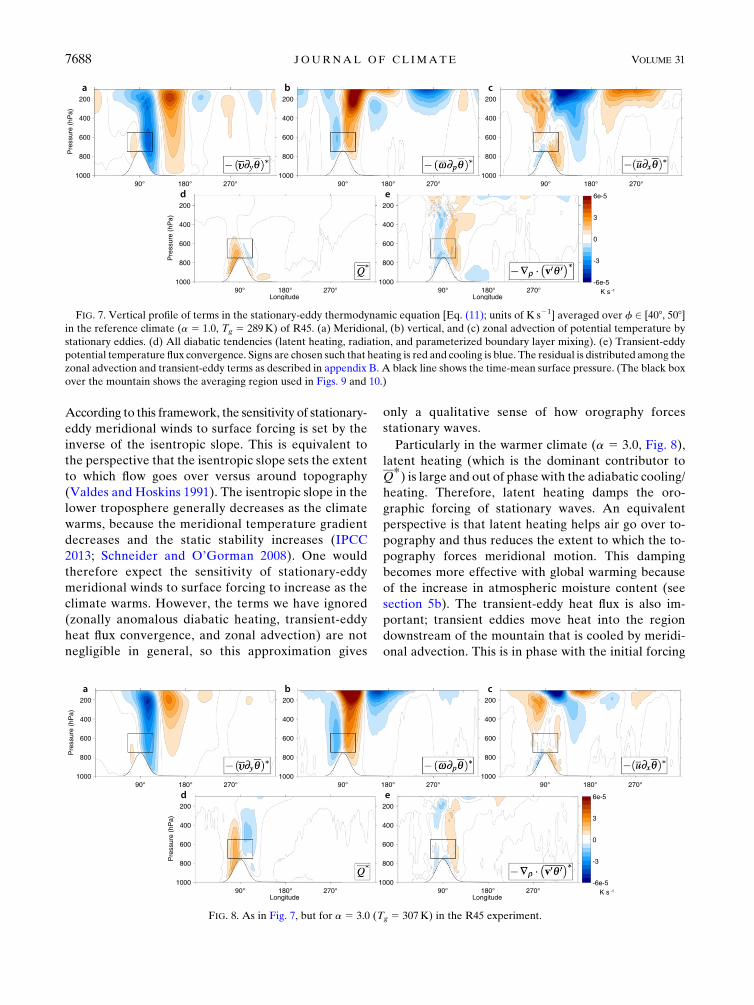
Particularly in the warmer climate (a 5 3.0, Fig. 8),

latent heating (which is the dominant contributor to

Q*) is large and out of phase with the adiabatic cooling/

heating. Therefore, latent heating damps the oro-

graphic forcing of stationary waves. An equivalent

perspective is that latent heating helps air go over to-

pography and thus reduces the extent to which the to-

pography forces meridional motion. This damping

becomes more effective with global warming because

of the increase in atmospheric moisture content (see

section 5b). The transient-eddy heat flux is also im-

portant; transient eddies move heat into the region

downstream of the mountain that is cooled by meridi-

onal advection. This is in phase with the initial forcing

FIG. 7. Vertical profile of terms in the stationary-eddy thermodynamic equation [Eq. (11); units of K s21] averaged over f 2 [408, 508]in the reference climate (a 5 1.0, Tg 5 289K) of R45. (a) Meridional, (b) vertical, and (c) zonal advection of potential temperature by

stationary eddies. (d) All diabatic tendencies (latent heating, radiation, and parameterized boundary layer mixing). (e) Transient-eddy

potential temperature flux convergence. Signs are chosen such that heating is red and cooling is blue. The residual is distributed among the

zonal advection and transient-eddy terms as described in appendix B. A black line shows the time-mean surface pressure. (The black box

over the mountain shows the averaging region used in Figs. 9 and 10.)

FIG. 8. As in Fig. 7, but for a 5 3.0 (Tg 5 307K) in the R45 experiment.


by adiabatic cooling/heating and thus amplifies the

stationary wave. This amplification becomes less ef-

fective with global warming because of decreases in

temperature gradients and transient-eddy kinetic en-

ergy (see section 5c). Zonal advection plays a similar

role to the transient-eddy heat fluxes in the lower tro-

posphere, but it is a weaker effect and will not be a

focus of this study.

To include these effects into a diagnostic theory for

y*2, we arrange the thermodynamic equation (11) into

an equation for y*,

y*’1

›yu(Q*2=

r� (v0u0)*2 u›

xu*2v*›pu)*. (15)

This equation simply states that, in the presence of

a meridional temperature gradient, the net heating

of zonal advection, vertical advection, transient-eddy

heat fluxes, and diabatic terms is balanced by me-

ridional advection. The only approximation applied

thus far is to assume that the stationary-eddy me-

ridional and vertical velocities, y* and v*, are larger

than the zonal-mean meridional and vertical veloci-

ties, [y] and [v]. We make a budget for y*2 by squaring

Eq. (15) to get

y*2 ’1

(›yu)2

(Q2 1Z2 1W2 2 2Q(Z1W)1 2ZW) ,

(16)

where Q[Q*2=r � (v0u0)*, Z[ (u›xu*)*, and

W[v*›pu.

We apply the meridional wind variance budget to

averages between 550 and 750hPa, within 58 latitude and258 longitude of the mountain center (denoted by f�g;shown by boxes in Figs. 7 and 8). The 750-hPa level is just

above the mountain in the time mean. Focusing on this

section of the lower troposphere allows us to diagnose

how the troposphere responds to the initial orographic

perturbation. The average stationary-eddy meridional

wind y* over these pressure levels is shown in Fig. 1b. The

climate change response of fy*2g is qualitatively similar

to the that of the global sEKE (Fig. 9a; cf. Fig. 3); it shows

an increase with warming up to 300-K global-mean sur-

face temperature and decrease with further warming

in the R45 experiment and a monotonic decrease with

warming in the R54 experiment. However, there are

quantitative differences between fractional fy*2g changesand fractional sEKE changes resulting from changes in

horizontal wind anisotropy and changes in the extent to

which Rossby waves propagate out of the orographic

forcing region.

To account for the effect of zonal variations in me-

ridional temperature gradients on the zonal variance

of y, we define an effective meridional temperature

gradient,

L2(f,p)5f(y*›

yu)2g

fy*2g , (17)

such that

fy*2g’ 1

L2fQ21Z2 1W22 2Q(Z1W)1 2ZWg. (18)

The hope is thatL behaves similarly to the zonal-mean

meridional temperature gradient j›y[u]jwith warming.

The effective meridional temperature gradient L is

larger than the zonal-mean meridional temperature

gradient j›y[u]j, due to strong local meridional temper-

ature gradients downstream of the mountain. However,

it shows a similar response to climate change (Fig. 9c).

The reduction in meridional temperature gradient with

global warming increases the meridional wind response

to a given forcing. To show the magnitude of this effect,

we plot L2fy*2g in Fig. 9a. It is scaled to match fy*2gin the reference climate such that it shows the fy*2gchanges that would result without any changes in me-

ridional temperature gradient. The role of the meridio-

nal temperature gradient in fy*2g changes can thus be

seen as the difference between the dashed and solid

black lines in Fig. 9a.

The temperature tendency variance terms on the right-

hand side of Eq. (18) make up a diagnostic for L2fy*2g,as shown in Fig. 9b. In both experiments, the variance

in adiabatic cooling/heating W2 is the largest term. It in-

creases with warming in R45 and decreases with warming

in R54, contributing to the differing responses of L2fy*2gin these experiments (blue lines in Fig. 9b).

The adiabatic cooling/heating term can be further

split up into influences from vertical velocity changes

and from stratification changes:

fW2g5G2fv*2g . (19)

Here, G characterizes the dry static stability felt by

stationary-eddy circulations,

G2(f,p)5f(v*›pu)2g

fv*2g [fW2gfv*2g . (20)

It is systematically smaller than the zonal-mean strati-

fication j›p[u]j in the coldest climates because the

lower-tropospheric (i.e., 750 hPa) temperature is ele-

vated in the vicinity of topography. It increases with

warming beyond 295-K global-mean surface tempera-

ture, roughly following changes in j›p[u]j (Fig. 9d). Thismeans that W2 changes are similar to those computed


FIG. 9. Factors controlling the meridional wind response to vertical motions and zonally anomalous heating. (a) Meridional wind

variance fy*2g across the range of climates in both experiments (solid black line with circles) and the meridional wind variance that would

result without changes in L (dashed line; L is fixed at its value in the reference climate, shown by the filled circle). (b) Variance of zonally

anomalous temperature tendencies, which contribute to changes in fy*2g according to Eq. (18) [see also Eq. (21)]. In each of these terms,

we leave off the factor ofL22 such that they sum toL2fy*2g, which is also shown in (a).Meridional temperature gradient changesmust also

be taken into account in deducing how these terms affect fy*2g. (c) Behavior of the zonal-mean meridional temperature gradient j›y[u]jand the effectivemeridional temperature gradientL across the range of climates. (d) Behavior of the zonal-mean dry static stability j›p[u]j,the effective static stability G (accounting for zonal anomalies in stratification), and the effective static stability Geff (accounting for zonal

anomalies in latent heating) across the range of climates. (e) Vertical wind variance fv*2g and a scaling that assumes it changes following

changes in v*2sfc, connecting the meridional wind variance budget to the analysis of the orographic vertical winds in section 4. Multiplying

fv*2g by G2 and G2eff recover the blue and cyan lines in (b). All averaging is done over the layer immediately above the mountain

(550–750 hPa) within 58 latitude and 258 longitude of the mountain.


from the vertical wind variance v*2 and the zonal-

mean stratification. The vertical wind variance v*2 scales

with the vertical surface wind variance vsfc*2 (Fig. 9e).

Therefore, the dominantW2 term is primarily determined

by the orographic vertical velocities (discussed in the

previous section) and the zonal-mean stratification,

which generally decreases in the midlatitudes as the

climate warms (Schneider and Walker 2008). The

adiabatic cooling and heating differs between the two

experiments primarily because of differences in oro-

graphic vertical velocity variance.

b. Latent heating

We analyze the effects of latent heating, transient

eddies, and zonal advection by grouping the remaining

terms according to

fy*2g’ 1

L2

8>>>><>>>>:W21Q*2

latent22Qlatent* W|fflfflfflfflfflfflfflfflfflfflfflfflfflfflffl{zfflfflfflfflfflfflfflfflfflfflfflfflfflfflffl}

latentheating

1Q*2trans22Q

trans* (W2Q

latent* )|fflfflfflfflfflfflfflfflfflfflfflfflfflfflfflfflfflfflfflfflfflfflfflffl{zfflfflfflfflfflfflfflfflfflfflfflfflfflfflfflfflfflfflfflfflfflfflfflffl}

transient2eddyheating

1Z21Q*2other12(Z2Q

other* )(W2Q

latent* 2Q

trans* )|fflfflfflfflfflfflfflfflfflfflfflfflfflfflfflfflfflfflfflfflfflfflfflfflfflfflfflfflfflfflfflfflfflfflfflfflfflfflfflfflfflffl{zfflfflfflfflfflfflfflfflfflfflfflfflfflfflfflfflfflfflfflfflfflfflfflfflfflfflfflfflfflfflfflfflfflfflfflfflfflfflfflfflfflffl}

other

9>>>>=>>>>;,

(21)

where Qtrans* [2=r � (v0u0)*. In anticipation of the can-

cellation between adiabatic cooling and latent heating,

we plot the net result of W2 and the latent heating term,

rather than the latent heating term by itself (cyan lines in

Fig. 9b). The latent heating term reduces the stationary-

eddy response throughout the range of climates. The

transient-eddy heating term (red lines in Fig. 9b) is

comparable in magnitude to the net forcing by vertical

motions and latent heating, and shows a large decrease

with climate change. It will be discussed in section 5c. The

zonal advection term Z and the other diabatic terms,

Qother* 5Qradiation

* 1Qsub-grid* , are small, but are needed for

quantitative accuracy (gray lines in Fig. 9b). These

terms are larger in the R45 experiment, where they

arise primarily because of the 2ZW term. This term

represents the influence of zonal advection down-

stream of the mountain, where zonal-mean westerlies

interact with a large cold anomaly (at approximately

1358 longitude), leading to heating to the west of the

cold anomaly and cooling to the east (Fig. 7c). This

heating (cooling) is in phase with the adiabatic cooling

(heating) by orographic vertical motions and acts to

strengthen the stationary wave.

The internal cancellation of adiabatic cooling and

latent heating in vertical motions is a common property

of circulations in moist atmospheres. One method to

account for this cancellation is to define an effective

static stability (Kiladis et al. 2009; O’Gorman 2011;

Cohen and Boos 2016; Nie et al. 2016). In this zonally

anomalous context, a requirement for defining an ef-

fective static stability is a strong correlation between

anomalies in adiabatic cooling2v*›p[u] and anomalies

in latent heating, such that

v*›p[u]2Qlatent* ’ «v*›p[u] . (22)

The correlation between adiabatic cooling and latent

heating ranges from 45% to 90% in these experiments,

with the best agreement in the warmest climates. The

effective static stability takes values of « 5 1 in the dry

limit, where latent heating is zero, and « 5 0 in the limit

where the adiabatic cooling is perfectly cancelled by la-

tent heating.

We quantify the effective static stability felt by sta-

tionary-eddy circulations by defining

G2eff(f, p)5

f(v*›pu2Qlatent* )

2gfv*2g [ «2G2 . (23)

Latent heating reduces the effective static stability felt by

stationary-eddy circulations throughout the range of cli-

mates (Fig. 9d). The difference between Geff and G gets

larger with warming as the moisture content of the atmo-

sphere increases and latent heating becomes a leading-

order thermodynamic term. While this result is qualita-

tively intuitive, it remains a challenge to relate « explicitly

to the moisture content of the atmosphere. As a conse-

quence, Geff remains an empirical parameter, diagnosed

from the simulations according to Eq. (23). In appendix B,

we provide a more detailed discussion of the mechanisms

leading to the correlation between zonally anomalous

adiabatic cooling and latent heating within orographic

stationarywaves [Eq. (22)], and their role in determining «.

The thermodynamic forcing of orographic stationary

waves by zonal anomalies in adiabatic cooling/heatingW2

is reduced by zonal anomalies in latent heating. The net

result, (W2Qlatent* )2, is related to the vertical wind vari-

ance byG2eff [Eq. (23)], which does not respond strongly to

climate change (Fig. 9d). Combined with changes in

vertical wind variance (Fig. 9e), the result is a near-

constant forcing by (W2Qlatent* )2 in the R45 experiment

and a strong monotonic decrease in (W2Qlatent* )2 in the

R54 experiment, the dominant factor in their differing

fy*2g responses.


c. Transient-eddy heat fluxes

The transient-eddy heating term is also important,

accounting for about half of the stationary-eddy ther-

modynamic forcing throughout the range of climates

(Fig. 9b). This amplification of stationary waves by

transient-eddy heat fluxes results from downgradient

heat fluxes into the cold region downstream of the

mountain (Figs. 7 and 8). Because this heat flux con-

vergence coincides with heating by adiabatic descent, it

is in phase with the initial forcing and acts to strengthen

the orographic stationary wave. The magnitude of the

temperature anomaly and the resulting transient-eddy

heat fluxes are proportional to the strength of the sta-

tionary-eddy winds, so these transient-eddy heat fluxes

can be thought of as a positive feedback on the strength

of stationary eddies. Note that we have not considered

transient-eddy momentum fluxes, which can modify

the climatological winds and overturning and thus

influence other thermodynamic terms. For example,

transient-eddy momentum fluxes likely play a role in

determining usfc* and thus vsfc* [Eq. (6)].

Transient-eddy heat fluxes act diffusively in the zonal

mean in that they increase as the pole–equator tem-

perature gradient increases (Held 1999; Caballero and

Langen 2005; Schneider and Walker 2008). If this were

the case for the zonally anomalous transient-eddy heat

fluxes in our idealized GCM experiments, the transient-

eddy heat flux convergence would be anticorrelated

with the zonal temperature anomaly. This is qualitatively

true, as shown by the downgradient heat fluxes into the

cold region downstream of the mountain (Figs. 7 and 8).

However, previous work has shown that this does not

lead to a simple functional relationship between zonal

temperature gradients and eddy fluxes (Lau andWallace

1979). Overall, there is a weak anticorrelation between

these quantities, but the transient-eddy heating has some

smaller-scale structure near the mountain related to the

enhanced meridional temperature gradient and the gen-

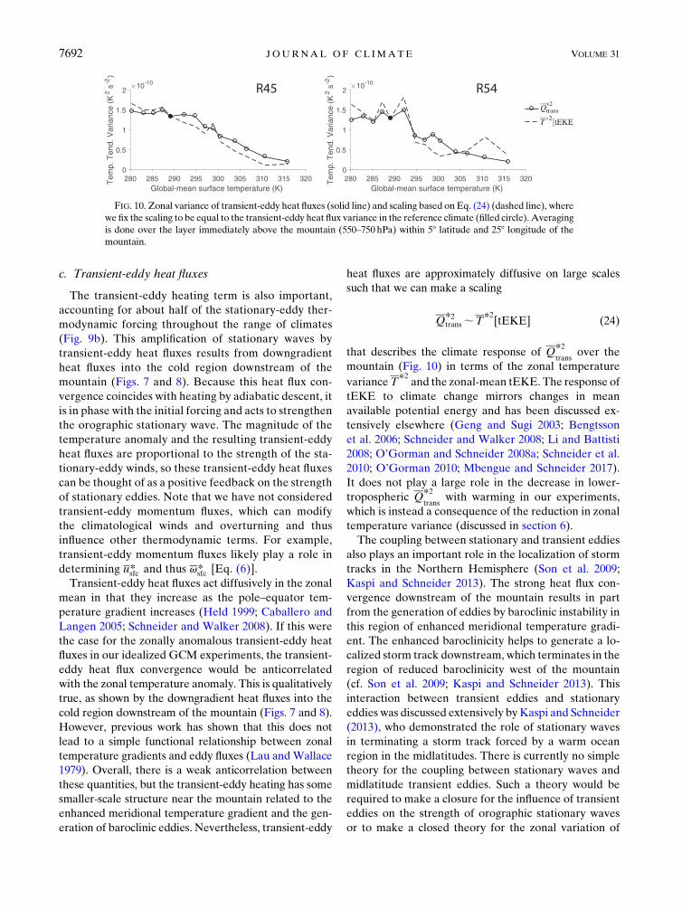
eration of baroclinic eddies. Nevertheless, transient-eddy

heat fluxes are approximately diffusive on large scales

such that we can make a scaling

Q*2trans ;T*

2[tEKE] (24)

that describes the climate response of Q*2trans

over the

mountain (Fig. 10) in terms of the zonal temperature

varianceT*2and the zonal-mean tEKE. The response of

tEKE to climate change mirrors changes in mean

available potential energy and has been discussed ex-

tensively elsewhere (Geng and Sugi 2003; Bengtsson

et al. 2006; Schneider and Walker 2008; Li and Battisti

2008; O’Gorman and Schneider 2008a; Schneider et al.

2010; O’Gorman 2010; Mbengue and Schneider 2017).

It does not play a large role in the decrease in lower-

tropospheric Q*2trans

with warming in our experiments,

which is instead a consequence of the reduction in zonal

temperature variance (discussed in section 6).

The coupling between stationary and transient eddies

also plays an important role in the localization of storm

tracks in the Northern Hemisphere (Son et al. 2009;

Kaspi and Schneider 2013). The strong heat flux con-

vergence downstream of the mountain results in part

from the generation of eddies by baroclinic instability in

this region of enhanced meridional temperature gradi-

ent. The enhanced baroclinicity helps to generate a lo-

calized storm track downstream, which terminates in the

region of reduced baroclinicity west of the mountain

(cf. Son et al. 2009; Kaspi and Schneider 2013). This

interaction between transient eddies and stationary

eddies was discussed extensively byKaspi and Schneider

(2013), who demonstrated the role of stationary waves

in terminating a storm track forced by a warm ocean

region in the midlatitudes. There is currently no simple

theory for the coupling between stationary waves and

midlatitude transient eddies. Such a theory would be

required to make a closure for the influence of transient

eddies on the strength of orographic stationary waves

or to make a closed theory for the zonal variation of

FIG. 10. Zonal variance of transient-eddy heat fluxes (solid line) and scaling based on Eq. (24) (dashed line), where

we fix the scaling to be equal to the transient-eddy heat flux variance in the reference climate (filled circle). Averaging

is done over the layer immediately above the mountain (550–750 hPa) within 58 latitude and 258 longitude of the

mountain.


transient-eddy variance, as exists in the Northern Hemi-

sphere storm tracks.

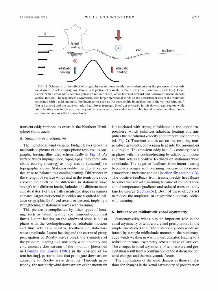
d. Summary of mechanisms

The meridional wind variance budget leaves us with a

mechanistic picture of the tropospheric response to oro-

graphic forcing, illustrated schematically in Fig. 11. As

surface winds impinge upon topography, they force adi-

abatic cooling (heating) as they ascend (descend) on

topographic slopes. Stationary-eddy meridional veloci-

ties arise to balance this cooling/heating. Differences in

the strength of surface winds and in the isentropic slope

account for much of the difference in stationary wave

strengthwith different forcing latitudes and differentmean

climate states. For the smaller isentropic slopes in warmer

climates, larger meridional velocities are required to bal-

ance orographically forced ascent or descent, implying a

strengthening of stationary waves with warming.

This picture is complicated by other types of heat-

ing, such as latent heating and transient-eddy heat

fluxes. Latent heating on the windward slope is out of

phase with the cooling/heating by adiabatic motions

and thus acts as a negative feedback on stationary

wave amplitude. Latent heating and the eastward group

propagation of Rossby waves break the symmetry of

the problem, leading to a northerly wind anomaly and

cold anomaly downstream of the mountain [described

in Hoskins and Karoly (1981) in the absence of la-

tent heating], perturbations that propagate downstream

according to Rossby wave dynamics. Through geos-

trophy, the northerly wind downstream of the mountain

is associated with strong subsidence in the upper tro-

posphere, which enhances adiabatic heating and am-

plifies the meridional velocity and temperature anomaly

(cf. Fig. 7). Transient eddies act on the resulting tem-

perature gradients, converging heat into the anomalous

cold region. The transient-eddy heat flux convergence is

in phase with the cooling/heating by adiabatic motions

and thus acts as a positive feedback on stationary wave

amplitude. The negative feedback from latent heating

becomes stronger with warming because of increased

atmospheric moisture content (section 5b; appendix B).

The positive feedback from transient-eddy heat fluxes

becomes weaker with warming because of reduced hori-

zontal temperature gradients and reduced transient-eddy

kinetic energy (section 5c). Both of these effects act

to reduce the amplitude of orographic stationary eddies

with warming.

6. Influence on midlatitude zonal asymmetry

Stationary-eddy winds play an important role in the

zonal asymmetry of temperature and precipitation. In the

simple case studied here, where stationary-eddy winds are

forced by a single midlatitude mountain, the stationary-

eddy winds weaken in warm, moist climates, leading to a

reduction in zonal asymmetry across a range of latitudes.

The changes in zonal asymmetry of temperature and pre-

cipitation result from a combination of the stationary-eddy

wind changes and thermodynamic factors.

The implications of the wind changes in these simula-

tions for changes in the zonal asymmetry of precipitation

FIG. 11. Schematic of the effect of orography on stationary-eddy thermodynamics in the presence of westerly

zonal winds (black arrows), overlain on a depiction of a single isotherm over the mountain (black line). Here,

a circle with a cross (dot) denotes poleward (equatorward) advection and upward and downward arrows denote

vertical motion. The response is asymmetric, with larger meridional winds on the downstream side of the mountain

associated with a cold anomaly. Nonlinear terms such as the geostrophic intensification of the vertical wind aloft

(big red arrow) and the transient-eddy heat fluxes (squiggly lines) act primarily in this downstream region, while

latent heating acts in the upstream region. Processes are color coded red or blue based on whether they have a

warming or cooling effect, respectively.


minus evaporation (P2E) have been discussed exten-

sively in WS16. There is a general tendency for the zonal

variance of P2E to increase as a result of the increase

in atmospheric moisture content. Superimposed on this

thermodynamic trend are any changes in stationary-eddy

circulations, as characterized by the lower-tropospheric

vertical winds (as shown in Fig. 9e). The zonal variance of

P2E thus increases with warming in moderate climates

before decreasing again at most latitudes in warm, moist

climates (Figs. 5 and 12 of WS16). Note that WS16 only

studied the R45 experiment; there is an even larger de-

crease in zonal P2E variance in the R54 experiment re-

sulting from the larger decreases in lower-tropospheric

vertical and horizontal winds (not shown).

Orographic vertical velocities exert a large influence

on orographic net precipitation (i.e.,P2E on orographic

slopes), through a term of the form

(P*2E*)orographic

’21

g(q

sfcvsfc* )* , (25)

where qsfc is the surface specific humidity (WS16). This

contribution to orographic net precipitation can be

further constrained by the scaling (7) for vsfc* in terms of

the zonal-mean zonal surface winds and surface pres-

sure gradients. However, as has been discussed in

WS16, zonally anomalous transient-eddy moisture

fluxes are large in the vicinity of topography. So while

the changes in time-mean vertical velocities are too

small to lead to much departure of orographic net

precipitation from Clausius–Clapeyron scaling, the

reduction in transient-eddy activity in the warmest

climates leads to a reduction in net precipitation over

orography (Fig. 12a ofWS16). In the real world, where

we expect a poleward migration of surface winds

with global warming (Kushner et al. 2001; Yin 2005),

the resulting changes in orographic vertical velocities

through the scaling (7) could play a role in amplifying

orographic P2E at high latitudes while reducing it at

lower latitudes.

Changes in the zonal variance of temperature also result

from a combination of dynamic and thermodynamic

factors. Based on a Taylor expansion, potential tem-

perature anomalies u* can to first order be expected to

depend on the zonal-mean meridional gradient of po-

tential temperature ›[u]/›y and a Lagrangian displace-

ment length L (Corrsin 1975; Schneider et al. 2015):

u*52L›[u]

›y. (26)

In the context of stationary eddies, L is the meridional

displacement of a time-mean streamline (Hoskins and

Woollings 2015). We examine the root-mean-square

(rms) of u* at the midlatitudes in our simulations, which

decreases with warming near the surface (Figs. 12a,b). It

should scale with the zonal-mean temperature gradient

according to

rms(u*);L

��›[u]›y

�� . (27)

The fractional reduction of the zonal-mean meridional

temperature gradient in the lower troposphere (Figs. 12c,d)

is comparable to the fractional reduction in rms(u*).

Accordingly, changes in the Langrangian displacement

length L, computed empirically, are small (Fig. 12e).

This is partially explained by the lack of changes in

stationary-eddy length scale in these simulations.

An alternative perspective is to think of the length

scaleL as the product of a velocity scale and a time scale

such that

rms(u*); t rms(y*)

��›[u]›y

�� . (28)

We have used the rms stationary-eddy meridional wind

rms(y*) as a velocity scale. The time scale t is the

Lagrangian decorrelation time of stationary eddies

(Swanson and Pierrehumbert 1997; Daoud et al. 2003)

and provides a time scale of the processes acting to re-

duce the temperature anomalies created by stationary-

eddy meridional advection, such as transient-eddy

heat fluxes, zonal advection, and radiation. Fractional

changes in rms(y*) at 850 hPa are small (Fig. 12f) com-

pared to fractional changes in the meridional tempera-

ture gradient. They are smaller than changes at higher

levels, but not considerably [cf. Fig. 9; note that y*2 is the

square of rms(y*)]. Changes in the empirical dissipation

time scale t are also small (Fig. 12g). Zonal temperature

variance changes are primarily determined by the re-

duction of the zonal-mean meridional temperature

gradient with warming, with only small contributions

from changes in dynamics, even in these idealized GCM

simulations that show large changes in stationary-eddy

winds across the range of climates. This is analogous

to the reduction in temporal temperature variance with

warming, which also results primarily from the reduc-

tion of the meridional temperature gradient rather

than dynamic factors (Schneider et al. 2015). It should

be kept in mind however, that a lack of dynamic influ-

ence on changes in zonal temperature variance does not

preclude a large dynamic influence on local changes in

temperature anomaly. Zonal temperature anomalies

are tightly coupled to the stationary-eddy winds and will

shift with shifting wind patterns.


7. Summary and conclusions

We have diagnosed the mechanisms governing the

strength of stationary Rossby waves forced bymidlatitude

orography across a wide range of climates in an idealized

GCM. To summarize, we group the most important in-

fluences on stationary wave amplitude by whether they

increase or decrease the amplitude with warming.

1) Nonmonotonic change with warming:d Change in zonal surface winds at the latitude of the

mountain.

2) Decreased stationary wave amplitude with warming:d Increased damping by latent heating.d Reduced zonal variation of transient-eddy heat

flux convergence as a result of reduced zonal

temperature variance (resulting primarily from a

reduced mean meridional temperature gradient)

and reduced tEKE (in the warmest climates).d Decreased top-of-mountain surface pressure due

to mean warming.

3) Increased stationary wave amplitude with warming:d Decreased isentropic slope resulting from increased

extratropical static stability and reduced meridional

temperature gradients.

The net result, after the internal cancellation of sev-

eral of these effects, is that the amplitude of orographic

stationary Rossby waves in these simulations scales

roughly with the zonal-mean zonal surface winds be-

cause of their influence on orographic vertical winds.

While the decrease in meridional temperature gradient

and increase in extratropical static stability would both

lead to an increased amplitude of orographic stationary

Rossby waves, the increased damping by latent heating

and reduced forcing by transient-eddy heat fluxes win

out to give a reduction in strength of orographic sta-

tionary Rossby waves with global warming. While the

relationship with zonal surface winds no longer applies

for simulations where orography is equatorward of the

band of surface westerlies, the same balance of phys-

ical mechanisms relates topographic vertical winds to

FIG. 12. (a) Root zonal variance of potential temperature rms(u*) at 850 hPa vs latitude in the R45 experiment and (b) an average over

mid-to-high latitudes f 2 [458, 908]. The zonal temperature variance decreases with warming. (c) Zonal-mean meridional temperature gra-

dient 2›y[u] at 850 hPa vs latitude in the R45 experiment and (d) an average over mid-to-high latitudes f 2 [458, 908]. The temperature

gradient decreases with warming. (e) The length scale obtained from dividing rms(u*) by2›y[u] at 850 hPa, which shows the lack of dynamic

changes in zonal temperature variance. (f) Root zonal variance of meridional velocity rms(y*) at 850 hPa. (g) The time scale obtained by

dividing the length scale in (e) by the velocity-scale rms(y*). All quantities in (e)–(g) are averaged over mid-to-high latitudes f 2 [458, 908].


the amplitude of orographic stationary Rossby waves

(Wills 2016).

In understanding the influence of stationary waves

on the zonal asymmetry of temperature and net pre-

cipitation, thermodynamic factors become leading or-

der. Reduced meridional temperature gradients are

associated with a reduction in the zonal asymmetry of

temperature. Increased atmospheric moisture content is

associated with an increase in zonal asymmetry of net

precipitation. However, the reduced amplitude of oro-

graphic stationary Rossby waves is an important factor

in reducing the zonal asymmetry of temperature and

precipitation in the warmest, wettest climates.

8. Implications

There are numerous important differences between the

idealized GCM used here and comprehensive models or

the real atmosphere. For example, the idealized GCM

simulates an equatorward shift of the surface westerlies

with global warming (Fig. 6) while comprehensive models

simulate a poleward shift (Yin 2005). However, all of the

mechanisms discussed herein emerge from the governing

physical equations and should have some relevance to the

real climate system. Which of them can we expect to be

important and which not? Because of the unusual equa-

torward shift of the surfacewesterlies, wedonot expect the

particular changes in surfacewinds and orographic vertical

velocities in theR45 andR54 experiments to apply to real-

worldmountain ranges at these latitudes.We do, however,

expect that the impinging zonal westerlies at the latitude of

the mountain are the relevant surface winds to determine

the strength of orographic forcing by midlatitude moun-

tains. This may remain true even in cases where the zonal

surface winds change sign, such as in the orographic forc-

ing of Rossby waves by the Zagros Mountains in summer

(Simpson et al. 2015).

In our simulations, the strength of the meridional

wind response to orographic perturbations scales with

the lower-tropospheric static stability and inversely with

the meridional temperature gradient. This is a simple

consequence of the thermodynamic equation and should

equally apply to the real world. As an example of these

mechanisms, recent work has shown that Mongolian to-

pography matters more for the wintertime atmospheric

circulation over the Pacific than the higher Tibetan Pla-

teau because of the stronger surface winds and larger

meridional temperature gradient at their higher latitude

(White et al. 2017). The expected increase in static sta-

bility and decrease in lower-tropospheric meridional

temperature gradients with global warming would both

lead to an increase in the strength of orographic station-

ary waves. However, latent heating and transient-eddy

heat fluxes must also be considered. In our simulations,

increased damping by latent heating and reduced re-

inforcement by transient-eddy heat fluxes limits the

strength of orographic stationary waves in warm cli-

mates. More work is needed to characterize latent

heating and transient-eddy feedbacks within stationary

waves in the real world.

Based on the mechanisms discussed in this study, the

response of orographic stationary Rossby wave ampli-

tude to climate change in the real climate system should

depend on the surface wind, meridional temperature

gradient, static stability, and latent heating changes in

key regions around large-scale orography, such as the

Rocky Mountains, Andes, Himalayas, Tibetan Plateau,

and Mongolia, as well as on interactions between sta-

tionary wave changes and storm track changes. Cloud

and water vapor feedbacks, which were not investigated

here, could provide an additional influence on the am-

plitude of orographic stationary Rossby waves, through

their role in the zonally anomalous energy budget, and

should be investigated in this context.

Acknowledgments. This work was primarily com-

pleted while both authors were at the Department of

Earth Sciences, ETH Zürich, Zurich, Switzerland. Thisresearch has also been supported by NSF Grant AGS-

1019211 while both authors were at the California

Institute of Technology, Pasadena, California. The ide-

alized GCM simulations for this study were performed

on ETH Zürich’s EULER computing cluster. Code for

the idealized GCM is available online (at https://github.

com/tapios/fms-idealized). We thank Simona Bordoni,

Andy Thompson, Jess Adkins, Rachel White, Momme

Hell, Farid Ait Chaalal, Ori Adam, and three anony-

mous reviewers for useful comments and discussion

during the development of this manuscript.

APPENDIX A

Interpolation to Pressure Coordinates

While the idealized GCM uses sigma coordinates, we

interpolate to pressure coordinates to avoid large spatial

gradients on sigma surfaces as the coordinate surfaces

slope over orography. The interpolation is done at every

6-hourly analysis time step, by linearly interpolating the

vertical integral of each quantity. This helps ensure that

mass is conserved in the interpolation. However, quanti-

ties with large vertical gradients, such as potential tem-

perature, can be shifted in the vertical direction, creating

large-amplitude grid-scale noise, which integrates to zero.

The residual of the thermodynamic equation (11) after

interpolation is shown in Fig. A1c. We distribute it to the


https://github.com/tapios/fms-idealized

https://github.com/tapios/fms-idealized

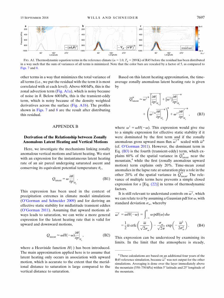
other terms in a way that minimizes the total variance of

all terms (i.e., we put the residual with the term it is most

correlated with at each level). Above 600 hPa, this is the

zonal advection term (Fig. A1a), which is noisy because

of noise in u. Below 600hPa, this is the transient-eddy

term, which is noisy because of the density weighted

derivatives across the surface (Fig. A1b). The profiles

shown in Figs. 7 and 8 are the result after distributing

this residual.

APPENDIX B

Derivation of the Relationship between ZonallyAnomalous Latent Heating and Vertical Motions

Here, we investigate the mechanisms linking zonally

anomalous vertical motions and latent heating. We start

with an expression for the instantaneous latent heating

rate of an air parcel undergoing saturated ascent and

conserving its equivalent potential temperature ue,

Qlatent

5v›u

›p

��ue

. (B1)

This expression has been used in the context of

precipitation extremes in climate model simulations

(O’Gorman and Schneider 2009) and for deriving an

effective static stability for midlatitude transient eddies

(O’Gorman 2011). Assuming that upward motions al-

ways leads to saturation, we can write a more general

expression for the latent heating rate that is valid for

upward and downward motions,

Qlatent

’vH(2v)›u

›p

��ue

, (B2)

where a Heaviside function H(�) has been introduced.

The main approximation applied here is to assume that

latent heating only occurs in association with upward

motion, which is accurate to the extent that the merid-

ional distance to saturation is large compared to the

vertical distance to saturation.

Based on this latent heating approximation, the time-

average zonally anomalous latent heating rate is given

by

Qlatent* ’v[*

"›u

›p

��ue

#1 [v[]

›u

›p

��ue

*

1 v[*›u

›p

��ue

*0@

1A*1v[0›u

›p

��0ue

*

, (B3)

where v[ 5vH(2v). This expression would give rise

to a simple expression for effective static stability if it

were dominated by the first term and if the zonally

anomalous gross upward mass flux v[* scaled with v*

(cf. O’Gorman 2011). However, the dominant term in

Eq. (B3) is the fourth (transient-eddy) term, which ex-

plains 60% of the spatial variance in Qlatent* near the

mountain,4 while the first (zonally anomalous upward

motion) term explains only 20%. Time-mean zonal

anomalies in the lapse rate at saturation play a role in the

other 20% of the spatial variance in Qlatent* . The rele-

vance of multiple terms here prevents a simple closed

expression for « [Eq. (22)] in terms of thermodynamic

factors.

It is still relevant to understand controls on v[, which

we can relate tov by assuming aGaussian pdf forv, with

standard deviation sv, whereby

v[ 5vH(2v) 5

ð 02‘

v pdf(v) dv

51

2v erfc

vffiffiffi2

psv

!2

svffiffiffiffiffiffi2p

p exp

�2

v2

2s2v

�. (B4)

This expression can be understood by examining its

limits. In the limit that the atmosphere is steady,

FIG. A1. Thermodynamic equation terms in the reference climate (a5 1.0, Tg5 289K) of R45 before the residual has been distributed

in a way such that the sum of variances of all terms is minimized. Note that the color bars are rescaled by a factor of 5, as compared to

Figs. 7 and 8.

4 These calculations are based on an additional four years of the

R45 reference simulation, because v[ was not output for the other

simulations. Averaging is done over the layer immediately above

the mountain (550–750 hPa) within 58 latitude and 258 longitude ofthe mountain.


v/sv /‘ and v[ /vH(2v): the time-mean gross

upward mass flux is given by the upward portion of the

time-mean vertical velocity. In the limit of no time-mean

vertical motion, v/sv / 0 and v[ /2sv/ffiffiffi2

pp: the

time-mean gross upward mass flux is proportional to the

standard deviation of the vertical velocity. The typical

time-mean vertical velocities near topography in these

simulations are about 0.05Pa s21, or approximately

5mms21, whereas a typical value for sv is 3–4 times that

(0.15–0.2 Pa s21). This means that zonal anomalies in v[

come in a large part from zonal anomalies in vertical

velocity statistics rather than from zonal anomalies in

the climatological vertical velocity v. Together with

the importance of the transient-eddy term in Eq. (B3),

this means that zonal anomalies in latent heating arise

through the interaction between transient and station-

ary eddies, rather than directly from stationary-eddy

vertical motions.

REFERENCES

Bender, F. A.-M., V. Ramanathan, and G. Tselioudis, 2012:

Changes in extratropical storm track cloudiness 1983–2008:

Observational support for a poleward shift. Climate Dyn., 38,

2037–2053, https://doi.org/10.1007/s00382-011-1065-6.

Bengtsson, L., K. I. Hodges, and E. Roeckner, 2006: Storm tracks

and climate change. J. Climate, 19, 3518–3543, https://doi.org/

10.1175/JCLI3815.1.

Boer, G. J., 1982: Diagnostic equations in isobaric coordinates.

Mon. Wea. Rev., 110, 1801–1820, https://doi.org/10.1175/

1520-0493(1982)110,1801:DEIIC.2.0.CO;2.

Brandefelt, J., and H. Körnich, 2008: Northern Hemisphere sta-

tionary waves in future climate projections. J. Climate, 21,

6341–6353, https://doi.org/10.1175/2008JCLI2373.1.

Broccoli, A. J., and S. Manabe, 1992: The effects of orography on

midlatitude Northern Hemisphere dry climates. J. Climate, 5,

1181–1201, https://doi.org/10.1175/1520-0442(1992)005,1181:

TEOOOM.2.0.CO;2.

Caballero, R., and P. L. Langen, 2005: The dynamic range of

poleward energy transport in an atmospheric general circu-

lation model. Geophys. Res. Lett., 32, L02705, https://doi.org/

10.1029/2004GL021581.

Chang, E. K. M., Y. Guo, and X. Xia, 2012: CMIP5 multimodel

ensemble projection of storm track change under global

warming. J. Geophys. Res., 117, D23118, https://doi.org/

10.1029/2012JD018578.

Charney, J. G., and P. G. Drazin, 1961: Propagation of planetary-

scale disturbances from the lower into the upper atmo-

sphere. J. Geophys. Res., 66, 83–109, https://doi.org/10.1029/

JZ066i001p00083.

Chen, J., and S. Bordoni, 2014: Orographic effects of the Tibetan

Plateau on the east Asian summer monsoon: An energetic

perspective. J. Climate, 27, 3052–3072, https://doi.org/10.1175/

JCLI-D-13-00479.1.

Chen, S.-C., and K. E. Trenberth, 1988: Orographically forced

planetary waves in the Northern Hemisphere winter: Steady

state model with wave-coupled lower boundary formula-

tion. J. Atmos. Sci., 45, 657–681, https://doi.org/10.1175/

1520-0469(1988)045,0657:OFPWIT.2.0.CO;2.

Cohen, N. Y., and W. R. Boos, 2016: Perspectives on moist bar-

oclinic instability: Implications for the growth of monsoon

depressions. J. Atmos. Sci., 73, 1767–1788, https://doi.org/

10.1175/JAS-D-15-0254.1.

Cook, K. H., and I. M. Held, 1988: Stationary waves of the ice

age climate. J. Climate, 1, 807–819, https://doi.org/10.1175/

1520-0442(1988)001,0807:SWOTIA.2.0.CO;2.

Corrsin, S., 1975: Limitations of gradient transport models in

random walks and in turbulence. Advances in Geophysics,

Vol. 18A, Academic Press, 25–60, https://doi.org/10.1016/

S0065-2687(08)60451-3.

Daoud,W. Z., J. D.W.Kahl, and J. K.Ghorai, 2003: On the synoptic-

scale Lagrangian autocorrelation function. J. Appl. Meteor., 42,

318–324, https://doi.org/10.1175/1520-0450(2003)042,0318:

OTSSLA.2.0.CO;2.

Deser, C., A. S. Phillips,M. A.Alexander, and B. V. Smoliak, 2014:

Projecting North American climate over the next 50 years:

Uncertainty due to internal variability. J. Climate, 27, 2271–

2296, https://doi.org/10.1175/JCLI-D-13-00451.1.

Egger, J., 1976: The linear response of a hemispheric two-level prim-

itive equation model to forcing by topography. Mon. Wea. Rev.,

104, 351–364, https://doi.org/10.1175/1520-0493(1976)104,0351:

TLROAH.2.0.CO;2.

Frierson, D. M. W., 2007: The dynamics of idealized convection

schemes and their effect on the zonally averaged tropical cir-

culation. J. Atmos. Sci., 64, 1959–1976, https://doi.org/10.1175/

JAS3935.1.

——, I. M. Held, and P. Zurita-Gotor, 2006: A gray-radiation

aquaplanet moist GCM. Part I: Static stability and eddy

scale. J. Atmos. Sci., 63, 2548–2566, https://doi.org/10.1175/

JAS3753.1.

Fyfe, J. C., 2003: Extratropical Southern Hemisphere cyclones: Har-

bingers of climate change? J. Climate, 16, 2802–2805, https://

doi.org/10.1175/1520-0442(2003)016,2802:ESHCHO.2.0.CO;2.

Geng, Q., and M. Sugi, 2003: Possible change of extratropical cy-

clone activity due to enhanced greenhouse gases and sulfate

aerosols—Study with a high-resolution AGCM. J. Climate, 16,

2262–2274, https://doi.org/10.1175/1520-0442(2003)16,2262:

PCOECA.2.0.CO;2.

Held, I. M., 1983: Stationary and quasi-stationary eddies in the

extratropical troposphere: Theory. Large Scale Dynamical

Processes in the Atmosphere, B. Hoskins and R. Pearce, Eds.,

Academic Press, 127–168.

——, 1993: Large-scale dynamics and global warming. Bull.

Amer. Meteor. Soc., 74, 228–241, https://doi.org/10.1175/

1520-0477(1993)074,0228:LSDAGW.2.0.CO;2.

——, 1999: The macroturbulence of the troposphere. Tellus, 51B,

59–70, https://doi.org/10.3402/tellusb.v51i1.16260.

——, and M. Ting, 1990: Orographic versus thermal forcing of

stationary waves: The importance of the mean low-level

wind. J. Atmos. Sci., 47, 495–500, https://doi.org/10.1175/

1520-0469(1990)047,0495:OVTFOS.2.0.CO;2.

——, R. L. Panetta, and R. T. Pierrehumbert, 1985: Stationary

external Rossby waves in vertical shear. J. Atmos. Sci., 42,

865–883, https://doi.org/10.1175/1520-0469(1985)042,0865:

SERWIV.2.0.CO;2.

——,M. Ting, andH.Wang, 2002: Northern winter stationary waves:

Theory and modeling. J. Climate, 15, 2125–2144, https://doi.org/

10.1175/1520-0442(2002)015,2125:NWSWTA.2.0.CO;2.

Hoskins, B. J., and D. J. Karoly, 1981: The steady linear response

of a spherical atmosphere to thermal and orographic forc-

ing. J. Atmos. Sci., 38, 1179–1196, https://doi.org/10.1175/

1520-0469(1981)038,1179:TSLROA.2.0.CO;2.


https://doi.org/10.1007/s00382-011-1065-6

https://doi.org/10.1175/JCLI3815.1


https://doi.org/10.1175/1520-0493(1982)110<1801:DEIIC>2.0.CO;2

https://doi.org/10.1175/1520-0493(1982)110<1801:DEIIC>2.0.CO;2

https://doi.org/10.1175/2008JCLI2373.1

https://doi.org/10.1175/1520-0442(1992)005<1181:TEOOOM>2.0.CO;2

https://doi.org/10.1175/1520-0442(1992)005<1181:TEOOOM>2.0.CO;2

https://doi.org/10.1029/2004GL021581

https://doi.org/10.1029/2004GL021581

https://doi.org/10.1029/2012JD018578

https://doi.org/10.1029/2012JD018578

https://doi.org/10.1029/JZ066i001p00083

https://doi.org/10.1029/JZ066i001p00083

https://doi.org/10.1175/JCLI-D-13-00479.1


https://doi.org/10.1175/1520-0469(1988)045<0657:OFPWIT>2.0.CO;2

https://doi.org/10.1175/1520-0469(1988)045<0657:OFPWIT>2.0.CO;2

https://doi.org/10.1175/JAS-D-15-0254.1


https://doi.org/10.1175/1520-0442(1988)001<0807:SWOTIA>2.0.CO;2

https://doi.org/10.1175/1520-0442(1988)001<0807:SWOTIA>2.0.CO;2

https://doi.org/10.1016/S0065-2687(08)60451-3

https://doi.org/10.1016/S0065-2687(08)60451-3

https://doi.org/10.1175/1520-0450(2003)042<0318:OTSSLA>2.0.CO;2

https://doi.org/10.1175/1520-0450(2003)042<0318:OTSSLA>2.0.CO;2


https://doi.org/10.1175/1520-0493(1976)104<0351:TLROAH>2.0.CO;2

https://doi.org/10.1175/1520-0493(1976)104<0351:TLROAH>2.0.CO;2

https://doi.org/10.1175/JAS3935.1




https://doi.org/10.1175/1520-0442(2003)016<2802:ESHCHO>2.0.CO;2

https://doi.org/10.1175/1520-0442(2003)016<2802:ESHCHO>2.0.CO;2

https://doi.org/10.1175/1520-0442(2003)16<2262:PCOECA>2.0.CO;2

https://doi.org/10.1175/1520-0442(2003)16<2262:PCOECA>2.0.CO;2

https://doi.org/10.1175/1520-0477(1993)074<0228:LSDAGW>2.0.CO;2

https://doi.org/10.1175/1520-0477(1993)074<0228:LSDAGW>2.0.CO;2

https://doi.org/10.3402/tellusb.v51i1.16260

https://doi.org/10.1175/1520-0469(1990)047<0495:OVTFOS>2.0.CO;2

https://doi.org/10.1175/1520-0469(1990)047<0495:OVTFOS>2.0.CO;2

https://doi.org/10.1175/1520-0469(1985)042<0865:SERWIV>2.0.CO;2

https://doi.org/10.1175/1520-0469(1985)042<0865:SERWIV>2.0.CO;2

https://doi.org/10.1175/1520-0442(2002)015<2125:NWSWTA>2.0.CO;2

https://doi.org/10.1175/1520-0442(2002)015<2125:NWSWTA>2.0.CO;2

https://doi.org/10.1175/1520-0469(1981)038<1179:TSLROA>2.0.CO;2

https://doi.org/10.1175/1520-0469(1981)038<1179:TSLROA>2.0.CO;2

——, and T. Woollings, 2015: Persistent extratropical regimes and

climate extremes. Curr. Climate Change Rep., 1, 115–124,

https://doi.org/10.1007/s40641-015-0020-8.

IPCC, 2013: Climate Change 2013: The Physical Science Basis.

Cambridge University Press, 1535 pp., https://doi.org/10.1017/

CBO9781107415324.

Joseph, R., M. Ting, and P. J. Kushner, 2004: The global stationary

wave response to climate change in a coupledGCM. J. Climate,

17, 540–556, https://doi.org/10.1175/1520-0442(2004)017,0540:

TGSWRT.2.0.CO;2.

Kaspi, Y., and T. Schneider, 2011: Winter cold of eastern conti-

nental boundaries induced by warm ocean waters.Nature, 471,

621–624, https://doi.org/10.1038/nature09924.

——, and ——, 2013: The role of stationary eddies in shaping

midlatitude storm tracks. J. Atmos. Sci., 70, 2596–2613, https://

doi.org/10.1175/JAS-D-12-082.1.

Kiladis, G. N., M. C. Wheeler, P. T. Haertel, K. H. Straub, and P. E.

Roundy, 2009: Convectively coupled equatorial waves. Rev. Geo-

phys., 47, RG2003, https://doi.org/10.1029/2008RG000266; Corri-

gendum, 49, RG3004, https://doi.org/10.1029/2011RG000370.

Kushner, P. J., I. M. Held, and T. L. Delworth, 2001: South-

ern Hemisphere atmospheric circulation response to global

warming. J. Climate, 14, 2238–2249, https://doi.org/10.1175/

1520-0442(2001)014,0001:SHACRT.2.0.CO;2.

Lau, N.-C., 1979: The observed structure of tropospheric stationary

waves and the local balances of vorticity and heat. J. Atmos. Sci.,

36, 996–1016, https://doi.org/10.1175/1520-0469(1979)036,0996:

TOSOTS.2.0.CO;2.

——, and J. M. Wallace, 1979: On the distribution of horizontal

transports by transient eddies in the Northern Hemisphere

wintertime circulation. J. Atmos. Sci., 36, 1844–1861, https://

doi.org/10.1175/1520-0469(1979)036,1844:OTDOHT.2.0.CO;2.

Li, C., and D. S. Battisti, 2008: ReducedAtlantic storminess during

Last Glacial Maximum: Evidence from a coupled climate

model. J. Climate, 21, 3561–3579, https://doi.org/10.1175/

2007JCLI2166.1; Corrigendum, 21, 6777, https://doi.org/

10.1175/JCLI2811.1.

Lutsko, N. J., and I. M. Held, 2016: The response of an idealized

atmosphere to orographic forcing: Zonal versus meridional

propagation. J. Atmos. Sci., 73, 3701–3718, https://doi.org/

10.1175/JAS-D-16-0021.1.

Mbengue, C., and T. Schneider, 2017: Storm-track shifts under

climate change: Toward a mechanistic understanding using

baroclinic mean available potential energy. J. Atmos. Sci., 74,

93–110, https://doi.org/10.1175/JAS-D-15-0267.1.

Molnar, P., W. R. Boos, and D. S. Battisti, 2010: Orographic con-

trols on climate and paleoclimate of Asia: Thermal and me-

chanical roles for the Tibetan Plateau. Annu. Rev. Earth Planet.

Sci., 38, 77–102, https://doi.org/10.1146/annurev-earth-040809-

152456.

Nie, J., D. A. Shaevitz, and A. H. Sobel, 2016: Forcings and feed-

backs on convection in the 2010 Pakistan flood: Modeling

extreme precipitation with interactive large-scale ascent.

J. Adv. Model. Earth Syst., 8, 1055–1072, https://doi.org/

10.1002/2016MS000663.

Nigam, S., I. M. Held, and S. W. Lyons, 1986: Linear simulation of

the stationary eddies in a general circulation model. Part I: The

no-mountain model. J. Atmos. Sci., 43, 2944–2961, https://

doi.org/10.1175/1520-0469(1986)043,2944:LSOTSE.2.0.CO;2.

——,——, and——, 1988: Linear simulation of the stationary eddies

in a GCM. Part II: The ‘‘mountain’’ model. J. Atmos. Sci., 45,

1433–1452, https://doi.org/10.1175/1520-0469(1988)045,1433:

LSOTSE.2.0.CO;2.

O’Gorman, P. A., 2010: Understanding the varied response of

the extratropical storm tracks to climate change. Proc. Natl.

Acad. Sci. USA, 107, 19 176–19 180, https://doi.org/10.1073/

pnas.1011547107.

——, 2011: The effective static stability experienced by eddies in a

moist atmosphere. J. Atmos. Sci., 68, 75–90, https://doi.org/

10.1175/2010JAS3537.1.

——, and T. Schneider, 2008a: Energy of midlatitude transient

eddies in idealized simulations of changed climates. J. Climate,

21, 5797–5806, https://doi.org/10.1175/2008JCLI2099.1.

——, and——, 2008b: The hydrological cycle over a wide range of

climates simulated with an idealized GCM. J. Climate, 21,

3815–3832, https://doi.org/10.1175/2007JCLI2065.1.

——, and ——, 2009: Scaling of precipitation extremes over a wide

range of climates simulated with an idealized GCM. J. Climate,

22, 5676–5685, https://doi.org/10.1175/2009JCLI2701.1.

Peixóto, J. P., and A. H. Oort, 1983: The atmospheric branch of the

hydrological cycle and climate. Variations in the Global Water

Budget, A. Street-Perrott, M. Beran, and R. Ratcliffe, Eds.,

Springer, 5–65.

——, and ——, 1992: Physics of Climate. American Institute of

Physics, 520 pp.

Ringler, T. D., and K. H. Cook, 1997: Factors controlling non-

linearity in mechanically forced stationary waves over orog-

raphy. J. Atmos. Sci., 54, 2612–2629, https://doi.org/10.1175/

1520-0469(1997)054,2612:FCNIMF.2.0.CO;2.

Rodwell, M. J., and B. J. Hoskins, 2001: Subtropical anticyclones

and summer monsoons. J. Climate, 14, 3192–3211, https://

doi.org/10.1175/1520-0442(2001)014,3192:SAASM.2.0.CO;2.

Schneider, T., and P. A. O’Gorman, 2008: Moist convection

and the thermal stratification of the extratropical tropo-

sphere. J. Atmos. Sci., 65, 3571–3583, https://doi.org/10.1175/

2008JAS2652.1.

——, andC. C.Walker, 2008: Scaling laws and regime transitions of

macroturbulence in dry atmospheres. J. Atmos. Sci., 65, 2153–

2173, https://doi.org/10.1175/2007JAS2616.1.

——, P. A. O’Gorman, andX. J. Levine, 2010:Water vapor and the

dynamics of climate changes. Rev. Geophys., 48, RG3001,

https://doi.org/10.1029/2009RG000302.

——, T. Bischoff, and H. Płotka, 2015: Physics of changes in

synoptic midlatitude temperature variability. J. Climate, 28,

2312–2331, https://doi.org/10.1175/JCLI-D-14-00632.1; Corri-

gendum, 29, 3471, https://doi.org/10.1175/JCLI-D-16-0096.1.

Shi, X., and D. R. Durran, 2014: The response of orographic pre-

cipitation over idealized midlatitude mountains due to global

increases in CO2. J. Climate, 27, 3938–3956, https://doi.org/

10.1175/JCLI-D-13-00460.1.

Simpson, I. R., T. A. Shaw, and R. Seager, 2014: A diagnosis of the

seasonally and longitudinally varying midlatitude circulation

response to global warming. J. Atmos. Sci., 71, 2489–2515,

https://doi.org/10.1175/JAS-D-13-0325.1.

——, R. Seager, T. A. Shaw, and M. Ting, 2015: Mediterranean

summer climate and the importance of Middle East topog-

raphy. J. Climate, 28, 1977–1996, https://doi.org/10.1175/

JCLI-D-14-00298.1.

——, ——, M. Ting, and T. A. Shaw, 2016: Causes of change in

Northern Hemisphere winter meridional winds and regional

hydroclimate. Nat. Climate Change, 6, 65–70, https://doi.org/

10.1038/nclimate2783.

Son, S.-W., M. Ting, and L. M. Polvani, 2009: The effect of topog-

raphy on storm-track intensity in a relatively simple general

circulation model. J. Atmos. Sci., 66, 393–411, https://doi.org/

10.1175/2008JAS2742.1.


https://doi.org/10.1007/s40641-015-0020-8

https://doi.org/10.1017/CBO9781107415324

https://doi.org/10.1017/CBO9781107415324

https://doi.org/10.1175/1520-0442(2004)017<0540:TGSWRT>2.0.CO;2

https://doi.org/10.1175/1520-0442(2004)017<0540:TGSWRT>2.0.CO;2

https://doi.org/10.1038/nature09924



https://doi.org/10.1029/2008RG000266

https://doi.org/10.1029/2011RG000370

https://doi.org/10.1175/1520-0442(2001)014<0001:SHACRT>2.0.CO;2

https://doi.org/10.1175/1520-0442(2001)014<0001:SHACRT>2.0.CO;2

https://doi.org/10.1175/1520-0469(1979)036<0996:TOSOTS>2.0.CO;2

https://doi.org/10.1175/1520-0469(1979)036<0996:TOSOTS>2.0.CO;2

https://doi.org/10.1175/1520-0469(1979)036<1844:OTDOHT>2.0.CO;2

https://doi.org/10.1175/1520-0469(1979)036<1844:OTDOHT>2.0.CO;2








https://doi.org/10.1146/annurev-earth-040809-152456

https://doi.org/10.1146/annurev-earth-040809-152456

https://doi.org/10.1002/2016MS000663

https://doi.org/10.1002/2016MS000663

https://doi.org/10.1175/1520-0469(1986)043<2944:LSOTSE>2.0.CO;2




https://doi.org/10.1073/pnas.1011547107

https://doi.org/10.1073/pnas.1011547107

https://doi.org/10.1175/2010JAS3537.1

https://doi.org/10.1175/2010JAS3537.1




https://doi.org/10.1175/1520-0469(1997)054<2612:FCNIMF>2.0.CO;2

https://doi.org/10.1175/1520-0469(1997)054<2612:FCNIMF>2.0.CO;2

https://doi.org/10.1175/1520-0442(2001)014<3192:SAASM>2.0.CO;2

https://doi.org/10.1175/1520-0442(2001)014<3192:SAASM>2.0.CO;2

https://doi.org/10.1175/2008JAS2652.1

https://doi.org/10.1175/2008JAS2652.1

https://doi.org/10.1175/2007JAS2616.1

https://doi.org/10.1029/2009RG000302








https://doi.org/10.1038/nclimate2783

https://doi.org/10.1038/nclimate2783

https://doi.org/10.1175/2008JAS2742.1

https://doi.org/10.1175/2008JAS2742.1

Stephenson, D. B., and I. M. Held, 1993: GCM response of northern

winter stationary waves and storm tracks to increasing amounts

of carbon dioxide. J. Climate, 6, 1859–1870, https://doi.org/

10.1175/1520-0442(1993)006,1859:GRONWS.2.0.CO;2.

Swanson, K. L., and R. T. Pierrehumbert, 1997: Lower-tropospheric

heat transport in the pacific storm track. J. Atmos. Sci., 54,

1533–1543, https://doi.org/10.1175/1520-0469(1997)054,1533:

LTHTIT.2.0.CO;2.

Ting, M., 1994: Maintenance of northern summer stationary waves

in a GCM. J. Atmos. Sci., 51, 3286–3308, https://doi.org/

10.1175/1520-0469(1994)051,3286:MONSSW.2.0.CO;2.

——, and L. Yu, 1998: Steady response to tropical heating in wavy

linear and nonlinear baroclinic models. J. Atmos. Sci., 55,

3565–3582, https://doi.org/10.1175/1520-0469(1998)055,3565:

SRTTHI.2.0.CO;2.

Toumi, R., N. Hartell, and K. Bignell, 1999: Mountain station

pressure as an indicator of climate change.Geophys. Res. Lett.,

26, 1751–1754, https://doi.org/10.1029/1999GL900351.

Valdes, P. J., and B. J. Hoskins, 1989: Linear stationary wave sim-

ulations of the time-mean climatological flow. J. Atmos. Sci., 46,

2509–2527, https://doi.org/10.1175/1520-0469(1989)046,2509:

LSWSOT.2.0.CO;2.

——, and ——, 1991: Nonlinear orographically forced planetary

waves. J. Atmos. Sci., 48, 2089–2106, https://doi.org/10.1175/

1520-0469(1991)048,2089:NOFPW.2.0.CO;2.

Vallis, G. K., 2006: Atmospheric and Oceanic Fluid Dynamics.

Cambridge University Press, 745 pp.

Vecchi, G. A., and B. J. Soden, 2007: Global warming and the

weakening of the tropical circulation. J. Climate, 20, 4316–

4340, https://doi.org/10.1175/JCLI4258.1.

Wang, L., and P. J. Kushner, 2011: Diagnosing the stratosphere-

troposphere stationary wave response to climate change in a

general circulation model. J. Geophys. Res., 116, D16113,

https://doi.org/10.1029/2010JD015473.

White, R. H., D. S. Battisti, and G. H. Roe, 2017: Mongolian

mountains matter most: Impacts of the latitude and height

of Asian orography on Pacific wintertime atmospheric cir-

culation. J. Climate, 30, 4065–4082, https://doi.org/10.1175/JCLI-D-16-0401.1.

Wills, R. C., 2016: Stationary eddies and zonal variations of the

global hydrological cycle in a changing climate. Ph.D. thesis,

California Institute of Technology, 177 pp.

——, and T. Schneider, 2015: Stationary eddies and the zonal

asymmetry of net precipitation and ocean freshwater

forcing. J. Climate, 28, 5115–5133, https://doi.org/10.1175/JCLI-D-14-00573.1.

——, and ——, 2016: How stationary eddies shape changes in the

hydrological cycle: Zonally asymmetric experiments in an

idealized GCM. J. Climate, 29, 3161–3179, https://doi.org/

10.1175/JCLI-D-15-0781.1.

——, M. P. Byrne, and T. Schneider, 2016: Thermodynamic and

dynamic controls on changes in the zonally anomalous hy-

drological cycle. Geophys. Res. Lett., 43, 4640–4649, https://doi.org/10.1002/2016GL068418.

——, X. J. Levine, and T. Schneider, 2017: Local energetic con-

straints on Walker circulation strength. J. Atmos. Sci., 74,1907–1922, https://doi.org/10.1175/JAS-D-16-0219.1.

Yin, J. H., 2005: A consistent poleward shift of the storm tracks in

simulations of 21st century climate. Geophys. Res. Lett., 32,

L18701, https://doi.org/10.1029/2005GL023684.


https://doi.org/10.1175/1520-0442(1993)006<1859:GRONWS>2.0.CO;2

https://doi.org/10.1175/1520-0442(1993)006<1859:GRONWS>2.0.CO;2

https://doi.org/10.1175/1520-0469(1997)054<1533:LTHTIT>2.0.CO;2

https://doi.org/10.1175/1520-0469(1997)054<1533:LTHTIT>2.0.CO;2

https://doi.org/10.1175/1520-0469(1994)051<3286:MONSSW>2.0.CO;2

https://doi.org/10.1175/1520-0469(1994)051<3286:MONSSW>2.0.CO;2

https://doi.org/10.1175/1520-0469(1998)055<3565:SRTTHI>2.0.CO;2

https://doi.org/10.1175/1520-0469(1998)055<3565:SRTTHI>2.0.CO;2

https://doi.org/10.1029/1999GL900351

https://doi.org/10.1175/1520-0469(1989)046<2509:LSWSOT>2.0.CO;2

https://doi.org/10.1175/1520-0469(1989)046<2509:LSWSOT>2.0.CO;2

https://doi.org/10.1175/1520-0469(1991)048<2089:NOFPW>2.0.CO;2

https://doi.org/10.1175/1520-0469(1991)048<2089:NOFPW>2.0.CO;2


https://doi.org/10.1029/2010JD015473







https://doi.org/10.1002/2016GL068418

https://doi.org/10.1002/2016GL068418


https://doi.org/10.1029/2005GL023684

Mechanisms Setting the Strength of Orographic Rossby Waves ...

Documents

Transcript of Mechanisms Setting the Strength of Orographic Rossby Waves ...