CHAPTER 4

DESIGNING AND SELECTING THE SAMPLE

This technical chapter1 is intended mainly for sample specialists, but also for the survey

coordinator and other technical resource persons. It will help you:

Determine the sample size Assess whether an existing sample can be used, or decide on an

appropriate sampling frame for a new sample Decide on the design of the new sample Gain awareness of issues related to subnational indicators and water and

sanitation estimates Become better informed about weighting, estimation and sampling errors Learn about pps sampling and implicit stratification Find out about sample designs used in three countries for the 2000 MICS

Conducting a Multiple Indicator Cluster Survey in your country will be carried out on a sample basis, as opposed to collecting data for an entire target population. There are different target populations in the survey – households, women aged 15 to 49 years, and children under five and in other age groups. The respondents, however, will usually be the mothers or caretakers of children in each household visited.2 It is important to recognize that MICS3 is a national-level survey and a sample from all households in the country will be chosen, not just those households that have young children or women of childbearing age.

DETERMINING THE SAMPLE SIZE The size of the sample is perhaps the most important parameter of the sample design, because it affects the precision, cost and duration of the survey more than any other factor. Sample size must be considered both in terms of the available budget for the survey and its precision 1 Users of the previous Multiple Indicator Cluster Survey Manual will note that this chapter is somewhat revised. Various changes include the formula for calculating sample size, greater emphasis on frame development and updating and on sampling error calculation, and inclusion of country examples from the year 2000 round of MICS. 2 A household is defined in the Multiple Indicator Cluster Survey as a group of persons who live and eat together. Any knowledgeable adult (defined, for the purposes of MICS3, as a person 15 years of age or older) is eligible to be the main respondent to the Household Questionnaire. However, in many cases, the respondent will be a mother or a primary caretaker for the practical reason that these individuals are more likely to be at home at the time of interview.

4.2 MULTIPLE INDICATOR CLUSTER SURVEY MANUAL requirements. The latter must be further considered in terms of the requirements for national versus subnational estimates. Moreover, the overall sample size cannot be considered independently of the number of sample areas – primary sampling units (PSUs) – and the size of the ultimate clusters. So, while there are mathematical formulas to calculate the sample size, it will be necessary to take account of all these factors in making your final decision.

Getting Help

This chapter of the manual, though fairly detailed, is not intended to make expert sampling statisticians of its readers. Many aspects of sample design will likely require assistance from a specialist, either from within the national statistics office or from outside. These aspects may include calculation of the sample size, construction of frame(s), evaluation of the sample design options, applying the pps sampling scheme, computation of the weights, and preparation of the sampling error estimates. In any case, it is strongly recommended that the national statistics office in your country be consulted on the design.

Two general rules of thumb govern the choice on the number of primary sampling units and the cluster sizes: the more PSUs you select the better, as both geographic representation, or spread, and overall reliability will be improved; the smaller the cluster size, the more reliable the estimates will be.

EXAMPLE: In a national survey, 600 PSUs with cluster sizes of 10 households each will yield a more reliable survey result than 400 PSUs with clusters of 15 households each, even though they both contain the same overall sample size of 6,000 households. Moreover, a cluster size of 10 is better than 15, because the survey reliability is improved with the smaller cluster size. In summary, it is better to strive for more rather than fewer PSUs, and smaller rather than larger clusters, provided other factors are the same.

In general, the more PSUs you select, the better your survey will be. However, the number of PSUs in your survey will be affected to a great extent by cost considerations and whether subnational estimates are needed (subnational estimates are discussed later in this chapter). Travel cost is a key factor. If the distances between PSUs are great and the same interviewing teams will be travelling from place to place (as opposed to using resident interviewers in each primary sampling unit), then decreasing the number of PSUs selected will significantly decrease overall survey costs. In contrast, if your survey requirements call for subnational estimates, there will be pressure on selecting more rather than fewer PSUs.

DESIGNING AND SELECTING THE SAMPLE 4.3 The choice of the cluster size is another parameter that has to be taken into account in determining sample size. Its effect can be assessed by the so-called sample design effect, or deff. The deff is a measure that compares the ratios of sampling variance from the actual stratified cluster survey sample (MICS3 in the present case) to a simple random sample3 of the same overall sample size. If, for example, the calculated value of the deff from the indicator survey were to be 2.0, this would tell you that the survey estimate has twice as much sampling variance as a simple random sample of the same size. Several specific examples of choosing the number of PSUs and deciding on the cluster size are given at the end of this section on sample size. The costs of simple random sampling preclude it from being a feasible option for MICS3 and for household surveys in general, which is why cluster sampling is used. The factors that contribute to sample design effects are stratification, the cluster size and the cluster homogeneity − the degree to which two persons (or households) in the cluster have the same characteristic. For example, the increased likelihood of two children living in close proximity both having received a given vaccination, compared to two children living at random locations in the population, is an example of cluster homogeneity. Stratification generally decreases sampling variance, while the homogeneity measure and the cluster size increase it. Hence, an objective in your sample design is to choose your cluster size so as to balance homogeneity, for which a smaller size is better, with cost, for which a larger size is usually better. To calculate the sample size for the survey, the design effect must be taken into account in the calculation formula. There are two problems, however. First, while the value of deff can be easily calculated after the survey, it is not often known prior to the survey, unless previous surveys have been conducted on the same variables. Second, the value of deff is different for every indicator and, in fact, every target group, because the cluster homogeneity varies by characteristic. It is not practical, of course, to conduct a survey with different sample sizes for each characteristic based on their variable deffs, even if we knew what they were. The deffs will not generally be known for indicators prior to the survey, but it is expected that they will be quite small for many indicators, that is, those based on rare subclasses (for example, children aged 12 to 23 months).4 If there has been a previous household survey that collected similar data to that of the MICS, and used a very similar sample design, you may be able to use the deffs from this previous survey to assess the likely design effects for MICS3. Few household

3 A type of probability sampling in which n sample units are selected with equal probability from a population of N units, usually without replacement and by using a table of random numbers. 4 The mathematical expression for deff is a function of the product of the cluster homogeneity and the cluster size. Even if the cluster size is large in terms of total households, it will be small in terms of this particular target population (1-year-old children), and so the deff is likely to be small also.

4.4 MULTIPLE INDICATOR CLUSTER SURVEY MANUAL surveys calculate design effects, but the Demographic and Health Surveys (DHS) project is one good source of such information. In the calculation formula and table for sample size in the following sections, we have assumed the design effect to be 1.5 (which may be somewhat high and therefore a conservative approach). In choosing a conservative deff, we want to ensure that the sample size will be big enough to measure all the main indicators. Nevertheless, a rule of thumb in choosing the cluster size and, by implication, the number of clusters is to make sure that the cluster size is as small as can be efficiently accommodated in the field, taking into account related considerations such as the number of PSUs and field costs (discussed above) and achieving interviewer workloads of a convenient size. CALCULATING THE SAMPLE SIZE To calculate the sample size, using the appropriate mathematical formula, requires that several factors be specified and values for others be assumed or taken from previous or similar surveys. These factors are:

• The precision, or relative sampling error, needed • The level of confidence desired • The estimated (or known) proportion of the population in the specified target group • The predicted or anticipated coverage rate, or prevalence, for the specified indicator • The sample deff • The average household size • An adjustment for potential loss of sample households due to non-response.

The calculation of sample size is complicated by the fact that some of these factors vary by indicator. We have already mentioned that deffs differ. Even the margin of error wanted is not likely to be the same for every indicator (and, in practice, it cannot be). This implies that different sample sizes would be needed for different indicators to achieve the necessary precision. Obviously, we must settle upon one sample size for the survey. The sample size calculation applies only to person-variables, even though it is expressed in terms of the number of households you must visit in order to interview individuals. This is because most of the important indicators for the MICS3 assessment are person-based. Household variables should not be used in the sample-size calculations because they require a different formula, as well as very different design effect (deff) values, as high as 10 or more.

DESIGNING AND SELECTING THE SAMPLE 4.5 The calculating formula is given by

[ 4 (r) (1-r) (f) (1.1) ] n = [ (0.12r)2 (p) (nh) ]

where

• n is the required sample size, expressed as number of households, for the KEY indicator (see following section on determining the key indicator)

• 4 is a factor to achieve the 95 per cent level of confidence • r is the predicted or anticipated prevalence (coverage rate) for the indicator

being estimated • 1.1 is the factor necessary to raise the sample size by 10 per cent for non-

response • f is the shortened symbol for deff • 0.12r is the margin of error to be tolerated at the 95 per cent level of

confidence, defined as 12 per cent of r (12 per cent thus represents the relative sampling error of r)

• p is the proportion of the total population upon which the indicator, r, is based, and

• nh is the average household size. If the sample size for the survey is calculated using a key indicator based on the smallest target group, in terms of its proportion of the total population, then the precision for survey estimates of most of the other main indicators will be better. Observant users of the MICS2 manual will notice that this formula differs in that relative sampling error (value of 0.12r) has been substituted for margin of error (e in the previous edition, with a value of either .05 or .03 for high and low coverage indicators, respectively). In the MICS2 manual, a reliable estimate for the survey was defined differently, depending upon whether it represents high or low coverage. For the indicator estimates, it was recommended that the margin of error, or precision, be set at 5 percentage points for rates of coverage (for example, immunizations) that are comparatively high, greater than 25 per cent, and at 3 percentage points for coverage rates that are low, 25 per cent or less. While a plausible rationale was given for presenting two margins of error defined in this way, users were nevertheless left with the often-difficult choice of which one to use for their survey, especially if the calculated sample sizes were widely different. By using the relative sampling error,5 this problem is avoided altogether because it scales the margin of error to result in comparable precision irrespective of whether a high coverage indicator or low coverage indicator is chosen as the key one for sample size determination. Note, however, that the sample size is nevertheless larger for low coverage 5 Statistically, the relative sampling error is known as the coefficient of variation and is defined as the standard error of a survey estimate divided by the estimate itself.

4.6 MULTIPLE INDICATOR CLUSTER SURVEY MANUAL indicators, which is why it is important to choose carefully which indicator is most key for the survey (see the following section). DEFINING AND CHOOSING THE KEY INDICATOR TO CALCULATE SAMPLE SIZE The recommended strategy for calculating the sample size is to choose an important indicator that will yield the largest sample size. This will mean first choosing a target population that comprises a small proportion of the total population (p in the above formula). This is generally a target population of a single-year age group.6 In MICS3, this is children aged 12 to 23 months, which in many MICS3 countries comprise about 2.5 per cent of the total population. We recommend using 2.5 per cent unless you have better estimates available for your country. If, for example, your figure is higher (3.5, 4 or 5 per cent) your sample sizes will be considerably less that those in Table 4.3, so it is very important to use your best estimate of p for this target population. Second, the particular indicator must be chosen for this same target population. We will label it the key indicator (but only for purposes of calculating the sample size).

Table 4.1

Indicator Coverage Rates, Prevalence or Proportion

Low coverage is undesirable • Use of improved water sources or sanitation facilities • School attendance • Antenatal care and institutional deliveries • Breastfeeding rates • Immunization coverage rates

Low coverage is desirable

• Mortality rates • Underweight, stunting or wasting prevalence • Child labour

In making your decision on the key indicator, you will need to choose one with low coverage. Some low coverage indicators should be excluded from consideration, however. This can be explained by reviewing the indicators in Table 4.1, where examples are given of indicators for which low coverage is undesirable and the associated goal is focused on raising the rate (for example, the immunization rate for DPT, that is, diphtheria, pertussis and tetanus). The second

6 In making your choice of the lowest-percentage population groups, it is strongly recommended that you exclude from consideration the four-month age groupings of children that form the basis for the breastfeeding indicators, because the necessary sample sizes would likely be impractically large.

DESIGNING AND SELECTING THE SAMPLE 4.7 set of indicators in Table 4.1 provides examples for which the opposite is true – low coverage is desirable and the goal is to lower it further (an example is stunting prevalence). It would not make sense to base your sample size on indicators for which low coverage is desired and coverage is already very low; such indicators should be excluded when picking the key indicator.

Table 4.2 provides suggestions for picking the target group and key indicator for purposes of calculating the sample size directly or finding the sample size in Table 4.3. Note that the infant mortality rate (IMR) or the maternal mortality ratio (MMR)7 are not mentioned as candidates for the key indicator. This is because the sample sizes that would be necessary to measure these indicators are much too large – in the tens of thousands – and it would be impractical to consider them. This does not necessarily mean that such indicators should not be measured in the survey, but rather that the sample size for the survey should not be based on them. The survey results for these indicators will have larger sampling errors and, hence, wider confidence intervals than the other indicators.

7 Regarding sample size for measuring the maternal mortality ratio: A 1997 guide by WHO and UNICEF entitled ‘The Sisterhood Method for Estimating Maternal Mortality’ recommends that if the maternal mortality ratio is 300 (per 100,000 live births), it can be estimated with a sample size of about 4,000 respondents with a margin of error of about 60, utilizing the indirect sisterhood method.

4.8 MULTIPLE INDICATOR CLUSTER SURVEY MANUAL

Table 4.2

Checklist for Target Group and Indicator

To decide on the appropriate target group and indicator that you need to determine your sample size: 1. Select two or three target populations that comprise small percentages of the

total population. Normally, these target groups should not be narrower than 1- year age groups, or wider than 5-year age groups. In MICS3, these will typically be children aged 12-23 months, or children under 5 years, which would, in many countries, comprise 2-4 per cent and 10-20 per cent of the total population, respectively.

2. Review important indicators based on these groups, ignoring indicators that have very low (less than 5 per cent) or very high (more than 50 per cent) prevalence. Begin calculations with your smaller group. If the indicators based on this group are high coverage, perform calculations for the wider age group, for which indicators might have lower coverage.

3. In general, pick an indicator that has a fairly low coverage rate for target populations comprising 10 to 15 per cent of the population, on the order of 15 or 20 per cent. For target populations comprising less than 5 per cent of the population, pick an indicator that has slightly higher coverage, above 20 per cent, but below 50 per cent.

4. Do not pick from the desirably low coverage indicators an indicator that is already acceptably low.

In making your choice, you must also consider the relative importance of the various indicators in your country. For example, you would not want to use an indicator that requires a very large sample size if that indicator is of comparatively small importance in your country. USING THE SAMPLE SIZE TABLE Table 4.3 shows sample sizes already calculated on the basis of MICS3 requirements, plus certain assumptions. You may use the table values, if they fit your situation, to get your sample size. Otherwise, you or your sampling specialist may calculate the sample size directly, using the formula given below. If the parameters in Table 4.3 fit the situation in your country, you can find the sample size without having to calculate it using the formula above. In Table 4.3, the level of confidence for the precision of the estimates is pre-specified at 95 per cent. Varying values of the average household size and coverage rate, r, are used – from 4.0 to 6.0 and from 0.25 to 0.40, respectively. The deff is assumed to be 1.5 and the precision (margin of error) level is set at 12 per cent of r, that is, a 12 per cent relative sampling error. The table reflects a 10 per cent upward adjustment in sample size to allow for potential non-response in the survey.

DESIGNING AND SELECTING THE SAMPLE 4.9 It is crucial to note that the table also assumes that the target population for your key indicator comprises 2.5 per cent of the total population. If it is a different value, you cannot use the table to find the required sample size. In general, the table cannot be used when any of the assumed values for the parameters of the formula do not fit your situation. More about what to do in this case is provided later in this section.

Table 4.3 Sample Size (Households) to Estimate Coverage Rates for Smallest Target Population

(with Relative Sampling Error of 12 Per cent of Coverage Rate at 95 Per cent Confidence Level)

Coverage Rates (r) Average Household Size (number of persons) r = 0.25 R = 0.30 R = 0.35 r = 0.40 4.0 13,750 10,694 8,512 6,875 4.5 12,222 9,506 7,566 6,111 5.0 11,000 8,556 6,810 5,500 5.5 10,000 7,778 6,191 5,000 6.0 9,167 7,130 5,675 4,583 Use this table when your

• Target population is 2.5 per cent of the total population; this is generally children aged 12-23 months • Sample design effect, deff, is assumed to be 1.5 and non-response is expected to be 10 per cent • Relative sampling error is set at 12 per cent of estimate of coverage rate, r

If all the assumptions for the parameter values of the formula pertain in your country, then one of the sample sizes in Table 4.3 should fit your situation. In some cases, the parameters may apply, but the coverage rate you choose has to be interpolated. For example, if your coverage rate is between 30 per cent and 35 per cent you may figure the sample size by interpolating a value between the third and fourth columns of the table. To illustrate: in the last row for a 32.5 per cent coverage rate, your sample size would be halfway between 7,130 and 5,675, or about 6,403 households. A stepwise illustration of the use of Table 4.3 can be given as follows:

• First, satisfy yourself that all the parameter values used in Table 4.3 apply in your situation.

• Next, from Table 4.2, pick the indicator that has the lowest coverage, excluding any indicator that is already acceptably low. Suppose it is measles immunization at 35 per cent.

• Next, find the average household size in Table 4.3 that is closest to that in your country (assuming it is within the ranges shown). Suppose it is 5.5 persons.

• Finally, find the value in Table 4.3 that corresponds to a household size of 5.5 persons and 35 per cent coverage rate. That value is 6,191.

4.10 MULTIPLE INDICATOR CLUSTER SURVEY MANUAL The figures should not, however, be taken as exact, but only as approximate sample sizes; remember that several assumptions were made in calculating the sample sizes. It would make sense to round the sample sizes up or down depending upon budget restraints. In this example, you might decide that 6,100 or 6,200 would be appropriate after you consider travel costs between primary sampling units, cluster sizes and interviewer workloads. USING THE SAMPLE SIZE FORMULA8 What happens to the sample size calculations if all the assumptions of the parameter values pertain, except that the proportion of children aged 12-23 months in your country is not 2.5 per cent, but instead is closer to 2.0 per cent? In that case, simply multiply all of the numbers in Table 4.3 by 2.5/2, or 1.25, to come up with the sample sizes. This is important since the sample sizes are significantly larger, an increase of 25 per cent. There are situations, however, when it is best to ignore Table 4.3 and calculate the sample size directly using the formula below. The formula must be used when any of the parameter values in your country differ from the assumptions used in Table 4.3. Table 4.4 outlines the conditions under which the formula should be used. We have already discussed why the sample size must be larger if p is smaller than 0.025. Unless the illustrated example above conforms to the situation in your country, the formula below should be used for calculating the sample size. To repeat, the formula below must be used if any of the other parameter values fit the criteria outlined in Table 4.4.

8 An Excel template for calculating sample size can be found at www.childinfo.org

DESIGNING AND SELECTING THE SAMPLE 4.11

Table 4.4

Checklist for Use of Sample Size Formula

The formula to determine your sample size is given by:

[ 4 (r) (1-r) (f) (1.1) ] n = [ (0.12r)2 (p) (nh) ]

Use it if any (one or more) of the following applies in your country: • The proportion of 1-year-old children (p) is other than 0.025 • The average household size (nh ) is less than 4.0 persons or greater than 6.0 • The coverage rate of your key indicator (r) is under 25 per cent • The sample design effect (f) for your key indicator is different from 1.5, according to

accepted estimates from other surveys in your country • Your anticipated non-response rate is more or less than 10 per cent.

Do not change the confidence level in the formula, but keep its value at 4.

Using the formula is quite easy, since it is basic arithmetic once the parameter values are inserted. For example, for r = 0.25, f = 1.6, non-response adjustment = 1.05, p = 0.035 and nh = 6, we have

[ 4 (0.25) (1-0.25) (1.6) (1.05) ] 1.26 n = [ (0.12 × 0.25)2 (0.035) (6) ] = 0.000189 = 6,667

In previous MICS surveys, the typical sample size has ranged between 4,000 and 8,000 households. That range is a plausible target for you to strive for when doing your calculations on sample size, considering both reliability requirements and budgetary constraints. As we mentioned already, MICS3 will produce estimates of many indicators, each of which will have its own level of precision. It is therefore useful to examine the approximate levels of reliability – standard errors and confidence limits – on your indicators for a particular sample size. Table 4.5 illustrates those levels of reliability for a sample of 6,000 households, which may be regarded as a typical sample size for producing comparatively reliable estimates for most indicators of interest in MICS3.

4.12 MULTIPLE INDICATOR CLUSTER SURVEY MANUAL

Table 4.5 Expected Reliability Measures (Standard Error and Confidence Interval) for Sample of

6,000 Households under Various Demographic Alternatives

Confidence interval (95% level)

Average household size

Size of indicator r

Size of subpopulation P

Number of sample persons in subpopulation

Number of persons with indicator

Standard error

Lower Upper

.025 540 54 .016 .068 .132

.05 1,080 108 .011 .078 .122

.125 2,700 270 .007 .086 .114

0.10

.20 4,320 432 .006 .089 .111

.025 540 108 .021 .158 .242

.05 1,080 216 .015 .170 .230

.125 2,700 540 .009 .181 .219

0.20

.20 4,320 864 .007 .185 .215

.025 540 162 .024 .252 .348

.05 1,080 324 .017 .266 .334

.125 2,700 810 .011 .278 .322

0.30

.20 4,320 1,296 .009 .283 .317

.025 540 270 .026 .447 .553

.05 1,080 540 .019 .463 .537

.125 2,700 1,350 .012 .476 .524

4

0.50

.20 4,320 2,160 .009 .481 .519

.025 675 68 .014 .072 .128

.05 1,350 135 .010 .080 .120

.125 3,375 338 .006 .087 .113

0.10

.20 5,400 540 .005 .090 .110

.025 675 135 .019 .162 .238

.05 1,350 270 .013 .173 .227

.125 3,375 675 .008 .183 .217

0.20

.20 5,400 1,080 .007 .187 .213

.025 675 203 .022 .257 .343

.05 1,350 405 .015 .269 .331

.125 3,375 1,013 .010 .281 .319

0.30

.20 5,400 1,620 .008 .285 .315

.025 675 338 .024 .453 .547

.05 1,350 675 .017 .467 .533

.125 3,375 1,688 .011 .479 .521

5

0.50

.20 5,400 2,700 .008 .483 .517

.025 810 81 .013 .074 .126

.05 1,620 162 .009 .082 .118

.125 4,050 405 .006 .088 .112

0.10

.20 6,480 648 .005 .091 .109

.025 810 162 .017 .166 .234

.05 1,620 324 .012 .176 .224

.125 4,050 810 .008 .185 .215

0.20

.20 6,480 1,296 .006 .188 .212

.025 810 243 .020 .261 .339

.05 1,620 486 .014 .272 .328

.125 4,050 1,215 .009 .282 .318

0.30

.20 6,480 1,944 .007 .286 .314

.025 810 405 .022 .457 .543

.05 1,620 810 .015 .470 .530

.125 4,050 2,025 .010 .481 .519

6

0.50

.20 6,480 3,240 .008 .485 .515

DESIGNING AND SELECTING THE SAMPLE 4.13 Column 4 in Table 4.5 shows the expected number of persons to be interviewed in a 6,000-household sample, assuming a non-response rate of 10 per cent. For example, in a country where the average household size is four persons, the number of sample persons in a subpopulation comprising 2.5 per cent of the total population (say, children aged 12-23 months) would be about 540, instead of 600, after allowing for non-response. Of those, column 5 shows the expected number of sample persons that would have the characteristic, r. The expected number of sample persons is 54 if r is 10 per cent, 108 if r is 20 per cent, 162 if r is 30 per cent, and 270 if r is 50 per cent. Observe that the expected standard error varies considerably depending on the size of the subpopulation and the size of the indicator. An important reliability measure for evaluating your results is the confidence interval, the last column in Table 4.5. The confidence interval, or CI, shows the range around which your estimate can be expected to vary from the true value in the population, taking account of the standard error. It is computed by adding and subtracting twice the standard error (for 95 per cent level of confidence) to the indicator estimate. Looking at the very last row of Table 4.5, the confidence interval shown is │0.485 - 0.515│for an indicator estimated at 0.50. This means that if you estimate the indicator coverage to be 50 per cent, then you can be confident with 95 per cent assurance that the true value of the indicator in the population is between 48.5 per cent and 51.5 per cent. DECIDING ON THE NUMBER OF PRIMARY SAMPLING UNITS AND CLUSTER SIZES – ILLUSTRATIONS At the beginning of the section on sample size, we discussed how the number of PSUs and the size of the clusters play a role in sample size. We emphasized that sampling reliability is improved with more PSUs and smaller cluster sizes. We conclude the section with three examples using different scenarios to illustrate the interrelationship of sample size, number of PSUs and cluster size. EXAMPLE 1:

Target group: Children aged 12 to 23 months Per cent of population: 2.6 per cent Key indicator: DPT immunization coverage Prevalence (coverage): 40 per cent Deff: No information Average household size: 6 Under this scenario, use Table 4.3 because the coverage rate of the key indicator and the household size can be found in the table. The target population, comprising 2.6 per cent, is also very close to the 3 per cent figure that Table 4.3 is based upon. With no information on the design effect, it is assumed to have a value of 1.5, and the non-response adjustment factor is assumed to be 1.1, corresponding to an expected 10 per cent non-response rate. The sample size for an average household size of 6.0 persons for a 40 per cent coverage rate is then found to be 4,583 households. Suppose that your country is relatively large in geographic size and, further, that there are

4.14 MULTIPLE INDICATOR CLUSTER SURVEY MANUAL

a large number of provinces, say, 15. You and your sampling staff have concluded, therefore, that you need to have a minimum of 300 PSUs in order to achieve good geographic spread and sufficient representation in each province. Moreover, you have decided that the budget for the survey would support that number of PSUs. The cluster size would then be calculated as 4,583 divided by 300, or about 15-16 households. Instead of targeting 300 PSUs as your number, you and the survey and sampling staff may have decided, alternatively, that you wanted clusters of a certain size, say, 10, in order to meet operational requirements such as interviewer workload distribution. In this case, you would divide 4,583 by 10 to give you the number of PSUs – about 458. You would then review this number in terms of cost and other considerations, and either accept it or adjust your cluster size. You might conclude that 425 is the maximum number of PSUs you can field because of travel costs, in which case you would have to adjust the cluster size to 11 (that is, 4,583/425).

EXAMPLE 2:

Target group: Children aged 12 to 23 months Per cent of population: 2.5 per cent Key indicator: Polio immunization coverage Prevalence (coverage): 26 per cent Deff: No information Average household size: 6 Under this scenario, you may still use Table 4.3 since, except for the coverage rate of the key indicator, all the parameters of the table pertain, given that we can again assume the design effect is 1.5 and non-response adjustment factor is 1.1. For coverage, r, we can use the column for 25 per cent since the estimated value of 26 per cent is so close. The sample size for an average household size of 6.0 persons is found in the table to be 9,167 households. Because of cost considerations and field workloads, suppose the survey team decides it wants cluster sizes of 30 households, if possible. Here, dividing 9,167 by 30 gives 306 PSUs, and you may decide that this is an acceptable number for the fieldwork. If, on the other hand, you decided that you would like to have about 400 PSUs for geographic spread and also to have enough PSUs to enable subnational estimates to be made for five regions, you would divide 9,167 by 400, which gives you 23 as your cluster size. Recall that the smaller the cluster size the more reliable the indicator estimates will be (for all indicators, not just the key indicator). You may decide, therefore, to use the 400-PSU design with its average cluster size of 23 households, bearing in mind that it will be more expensive than 306 PSUs due to travel costs.

EXAMPLE 3:

Target group: Children aged 0 to 11 months Per cent of population: 3.5 per cent Key indicator: Adequately fed infants Prevalence (coverage): 24 per cent Deff: 1.4 (from a previous survey) Average household size: 4 Expected non-response rate 10 per cent Under this scenario, you would have to calculate the sample size by using the formula provided in this section, since several of the parameters differ from those used or

DESIGNING AND SELECTING THE SAMPLE 4.15

assumed in Table 4.3. They include the values for p, f and the non-response adjustment factor, the latter of which is based on an expected non-response rate of 5 per cent instead of 10 per cent, judging from similar surveys in your country. The formula yields a figure of 10,303 households. Suppose that the survey staff has concluded that the survey can handle a maximum of 300 PSUs because of cost considerations. In this case, you would set 300 as fixed and figure the cluster size by dividing 10,303 by 300, which gives 34 households as the cluster size. Here you would have to evaluate whether a cluster size that big will give sufficiently reliable estimates for indicators other than the key ones.9 If we assume that the maximum cluster size should not be greater than 30 households, the number of PSUs that would be needed for 10,303 households is 343. Thus, the choice would have to be made whether to accept the lower reliability on a 300-PSU design or the higher cost of a 343-PSU design.

DETERMINING WHAT SAMPLE TO USE Once you have decided on the sample size and made initial determinations about the number of PSUs, the next task is to decide what sample to use for the survey. Designing, selecting and implementing a proper probability sample from beginning to end is a time-consuming and expensive process (probability sampling is discussed in the next section). For MICS3, there is the need to produce the indicator estimates in a comparatively short time frame, and you may not have sufficient time to design a new sample for the survey. Hence, there are two major steps to be followed in determining what sample to use for your survey: Step 1: Determine if an existing sample can be used. Step 2: If no suitable existing sample can be found, develop a sample specific to MICS3. In this section we discuss step 1. If there is a suitable existing sample for MICS3, you need not review the optional sample designs presented for step 2, which is discussed in the next section. It is nevertheless useful to review the next section in order to assure yourself that the existing sample you plan to use is a proper probability sample with a reasonably current sampling frame.

9 While the design effect is very low for the key indicator of this example, and hence the reliability of that estimate would be expected to meet the precision requirements set, other indicators that have a much higher intra-cluster correlation than that for children under age one would be expected to have considerably higher sampling errors with a cluster size over 30 compared to, say, 20 or 25.

4.16 MULTIPLE INDICATOR CLUSTER SURVEY MANUAL USE OF AN EXISTING SAMPLE – OPTION 1 Fortunately, most countries have well-developed survey programmes through their national statistical offices or health ministries. It may be possible in your country, therefore, to use an already existing sample, one that has been designed for other purposes. This is the recommended option for your survey if the existing sample is a valid probability sample and is available. The existing sample must be evaluated to see if it meets the requirements of probability sampling (which is discussed in a subsequent section).

There are various ways in which an existing sample may be used: • Attaching MICS3 questionnaire modules to the questionnaires to be used in

another survey • Using the sample, or a subset, from a previous survey • Using the household listings in the sample enumeration areas (or clusters) of

another survey • Using the enumeration areas or clusters from a previous survey with a fresh

listing of households.

Of these choices, there are advantages and limitations to each. Timing considerations are also a key factor. For example, the first choice is only an option if another survey is going to be carried out within the prescribed time frame for the MICS. This choice – attaching the questionnaire modules to another survey, sometimes called ‘piggy-backing’ because the data for both surveys are collected simultaneously – has obvious appeal since the sampling will have already been done, thus saving the sampling costs for MICS3. A major limitation, however, can be the burden it places on the respondent, since MICS3 questionnaires are quite long and the parent survey may have its own lengthy questionnaire. These aspects must be carefully evaluated and discussed with the host survey sponsors and management team. The second choice, using the sample from a previous survey, also has the advantage that the sample design is already in place, again saving sampling costs. If the sample size for the previous survey was too large, it would be a simple matter for the sampling statistician to sub-sample the original sample to bring the size into compliance with MICS3 requirements. By contrast, however, if the sample size is too small, expanding it is more problematic. There is also the limitation of revisiting the same households from the previous survey, again because of potential problems this could pose in terms of respondent burden and/or conditioning. Finally, the previous survey must be very recent for this to be a viable choice. The third choice, using the household listings in sample enumeration areas from a previous survey as a frame for selecting the MICS3 sample, has a dual advantage: (1) the first-stage units are already sampled and (2) household listings are already available. Therefore, again, most of the sampling operations and costs will already have been achieved. An advantage is that different households would be selected for MICS3, thus eliminating the problems of respondent burden, fatigue or

DESIGNING AND SELECTING THE SAMPLE 4.17 conditioning. A limitation is that the household listings would be out of date if the previous survey is more than a year or two old, in which case this choice would not be viable. In fact, when the household listings are out of date, then the fourth choice above can be considered. This choice requires making a fresh listing of households in the sample enumeration areas before sample selection. While this has the limitation of having to carry out a new household listing operation, with its associated expense, the advantage is that first-stage units would have already been selected and the sample plan itself is basically in place without further design work.

Table 4.6

Option 1 – Existing Sample Pros • Saves time and cost • Likely to be properly designed with probability methods • Adjustments to fit MICS3 can be simple Cons • Requires updating if old • Respondents may be overburdened • Indicator questionnaire may be too long if ‘piggy-backed’ • Adjustments to fit MICS3 can be complex

Each of these points should be carefully evaluated and a determination made about the feasibility of implementing the necessary modifications before you decide to use an existing sample. An existing sample that may be an excellent candidate is the Demographic and Health Survey (DHS).10 Many countries have conducted these surveys recently and others plan to in the coming months.11 The measurement objectives of DHS are quite similar to the MICS. For that reason, the sample design that is used in DHS is likely to be perfectly appropriate for your use. Under what circumstances is it appropriate to use the DHS sample? You must evaluate its availability, timeliness and suitability in terms of your requirements. Either a recent but pre-2003 DHS sample could be used to field the MICS, or an upcoming DHS could be used with the MICS3 as a supplement. The DHS will undoubtedly be designed as a probability sample. Therefore, you need only evaluate whether (1) its sample size is large enough for MICS and (2) 10 Sampling matters are described in Demographic and Health Surveys: Sampling Manual, Basic Documentation – 8. Calverton, Maryland: Macro International Inc., 1987. 11 It should be noted, however, that conducting MICS3 is not recommended if a DHS has been done since 2003, or will be done in 2005 or early 2006.

4.18 MULTIPLE INDICATOR CLUSTER SURVEY MANUAL the number of PSUs and cluster sizes are within the ranges that are discussed in this manual. Finally, it would require agreement and cooperation with the DHS sponsoring or implementing agency in your country, noting the constraints mentioned above about overburdening respondents. Another survey that many countries have implemented and whose sample may be appropriate for your use is a labour force survey. While the measurement objectives of labour force surveys are quite different from the objectives of MICS3, labour force surveys are frequently designed in a very similar fashion to Multiple Indicator Cluster Surveys in terms of stratification, sample size and other sampling criteria.

DEVELOPING A SAMPLE FRAME FOR A NEW SAMPLE When an existing sample cannot be used, it will be necessary to use and/or develop a sampling frame of households from which to select a new sample for MICS3. The frame should be constructed in accordance with the tenets of probability sampling. PROPER PROBABILITY SAMPLING DESIGN AND SAMPLING FRAME Design of an appropriate probability sample for the survey is just as important as development of the various questionnaire modules in terms of producing results that will be valid and, as far as possible, free from bias. There are a number of ways you can design a probability sample, and each country will undoubtedly have its own conditions and data needs that dictate the particular sample plan it adopts. There are certain features that should be observed by all countries, however, to meet the requirements of a scientific probability sample:

• Use accepted probability sampling methods at every stage of sample selection • Select a nationally representative sample • Ensure that the field implementation is faithful to the sample design • Ensure that the sample size is sufficient to achieve reliability requirements.

In addition to these four requirements, there are other features of sample design that you are strongly recommended to adopt, although each may be modified in certain ways depending upon country situations and needs. They include:

• Simple, as opposed to complex, sampling procedures • Use of the most recent population census as the sampling frame • A self-weighting sample, if possible.

DESIGNING AND SELECTING THE SAMPLE 4.19 Scientifically grounded probability sampling methods for surveys have been practised in most countries of the world for decades. If a sample is not accurately drawn from the whole population of interest by using well-known probability techniques, the survey estimates will be biased. Moreover, the magnitude of these biases will be unknown. It is crucial to ensure that the sampling methodology employs probability selection techniques at every stage of the selection process. Probability sampling is a means of ensuring that all individuals in the target population12 have a known chance of being selected into the sample. Further, that chance must be non-zero and calculable. A sure sign of not having a probability sample is when the sampling statistician cannot calculate the selection probabilities of the sample plan being used. Examples of sampling methods that are not based on probability techniques are judgement samples, purposive samples and quota samples. The random walk method of selecting children is a quota sample procedure. It is important that you not use such procedures for MICS3. The best way to control sampling bias is to insist on strict probability sampling. There are other biases, non-sampling in origin, including non-response, erroneous response, and interviewer errors, but these will occur in varying degrees anyway, no matter what kind of sampling methods are used. Appropriate steps must be taken to control these non-sampling biases as well, including such measures as pre-testing, careful interviewer training and quality control of fieldwork. A second required feature of sample design for MICS3 is that the sample should be national in scope and coverage. This is necessary because the indicator estimates must reflect the situation of the nation as a whole. It is important to include, to the extent practicable, difficult-to-enumerate groups to ensure complete national coverage. Such groups might be nomads, homeless or transient persons, or those living in refugee camps, military quarters, as well as settlements in isolated areas that are difficult to access. It is quite likely that children in particular, living in such situations, have different health conditions from those found in more

12 MICS3 has different target populations depending upon the indicator. Examples include children aged 0 to 11 months, 12 to 23 months, under 5 years, children under 5 years with diarrhoea, women aged 15 to 49 years, and the total population.

To avoid sample bias, you should use probability sampling to select the respondents. Sample bias depends on the selection techniques, not the sample size. Increasing the sample size will not eliminate sample bias if the selection techniques are wrong.

In probability samples, every person in the target population has a chance of being selected, the selection chance is non-zero and is calculable mathematically, and probability techniques are used in every stage of selection.

4.20 MULTIPLE INDICATOR CLUSTER SURVEY MANUAL stable or traditional living environments, and excluding them would result in biased indicator estimates. One of the crucial ways in which the sample can be truly national in scope and therefore consistent with proper probability sampling is by ensuring that the frame used covers the entire population of the country. The sampling frame is discussed in more detail below. For probability sampling to be effective, it is essential that the field implementation of the sample selection plan, including the interviewing procedures, be faithful to the design. There have been numerous occasions where lax fieldwork has ruined an otherwise perfectly acceptable sample design. The field supervisors must make certain that the sample selection procedures are followed strictly. A crucial feature of valid probability sampling is the specification of precision requirements in order to calculate the sample size. This topic was discussed in the previous section on determining sample size. We have recommended that the precision for the key indicator be set at a relative sampling error of 12 per cent at the 95 per cent level of confidence, and those are the criteria under which the calculation formula for sample size is based. If your key indicator is, for example, one with 20 per cent coverage or prevalence, then the 12 per cent relative error translates into a margin of error of 2.4 percentage points, and the confidence interval on your survey estimate of 20 per cent would be │17.6 – 22.4│. Your sample should be designed as simply as possible. It is well known that the more complex the sample plan is, the more likely it is that its implementation will go wrong. This can be especially troublesome at the field level if complicated sampling procedures have to be carried out. Moreover, the operational objective to produce the survey results in a timely manner may not be met. A sample plan is said to be self-weighting when every sample member of the target population is selected with the same overall probability. The overall probability is the product of the probabilities at each of the stages of selection. A self-weighting sample is desirable because various estimates can be prepared, for example, percentage distributions, from the sample figures without weighting, or inflating, them. In keeping with the desire for simplicity in sample design, it is better to have a self-weighting design than a more complicated, non-self-weighting one. Still, self-weighting should not be considered a strict criterion, because weighting the sample results to prepare the estimates can be easily handled by today’s computers. Moreover, there are some situations where the sample design cannot be self-weighting.

DESIGNING AND SELECTING THE SAMPLE 4.21

EXAMPLE: Suppose that in your country you will need separate urban and rural indicator estimates, and suppose further that you want the estimates to be equally reliable. This would necessitate selecting a sample of equal size in the urban and rural sectors. Unless the urban and rural populations are equal, the sampling rates in each would be different. Hence, the overall national sample would require weighting for correct results and, therefore, the survey sample would not be self-weighting.

CENSUS SAMPLING FRAME AND WHEN UPDATING BECOMES NECESSARY It is strongly recommended that the most recent population census be used as the basis for the sample frame, updated if necessary. Nearly all countries of the world now have a recent population census, that is, one conducted within the last 10 years. The frame is essentially the set of materials from which the survey sample is selected. A perfect sampling frame is one that is complete, accurate and up to date, and while no frame is 100 per cent perfect, the population census comes closest in most countries. The prime use of the census for our survey is to provide a complete list of enumeration areas with measures of size, such as population or household counts, for selection of the first-stage sampling units. Maps are usually part of the census of population in most countries, and these might include sketch maps for the enumeration areas. The maps are a useful resource because the selected enumeration areas will likely have to be updated in terms of the current households residing therein, especially if the census is more than a year or two old. Some countries conducted their year 2000 round of censuses as early as 1999, while many others conducted theirs during the period 2000-2002. This brings us to the very important issue of whether the census frame will need to be updated for MICS. It is recommended, in general, that updating not be undertaken if the census frame was created in 2003 or later, with one exception. In countries where there have been dramatic shifts in population since 2003, especially in highly urbanized areas that have expanded in specific zones due to massive new construction of residential units, an updating operation should be undertaken in such zones. You may decide, however, that this is not necessary if your population census is so recent that it precedes your survey by 12 months or less. The reason for updating is probably apparent. It is necessary to ensure that coverage of the total population is as accurate and complete as possible. The recommended steps for updating the census frame are the same under either scenario, that is, whether in large-scale urban developments since 2003 or for general updating of an old census frame prepared prior to 2003. The difference is in the scope and scale of the updating operation. Updating an old, pre-2003, census frame is considerably more demanding and expensive than updating the more recent frames. In either case, however, the operation must take place for the entire sampling frame and

If the census frame in your country was prepared before 2003, updating is recommended.

4.22 MULTIPLE INDICATOR CLUSTER SURVEY MANUAL not just those enumeration areas – PSUs – that happen to be selected in the sample. In fact, the information gathered in updating is used to select the sample. It is important to be aware that updating a frame is a major statistical operation. If updating becomes necessary, it cannot be ignored in your costing algorithm when you are preparing your budget. Moreover, you are strongly urged to engage the services of your national statistical office when updating is deemed necessary. The specific steps are as follows:

1. Identify the zones, especially in large cities, where there has been massive residential construction since the census was conducted, irrespective of whether your population census is pre- or post-2003.

2. Identify new zones, such as squatter communities that have become highly populated since the census. These may include zones that were ‘empty’ or very sparsely populated at the time of the census.

3. Ignore old, stable residential zones where little change occurs over time. 4. Match the zones identified in steps 1 and 2 with their census enumeration areas, taking

into account overlapping boundaries. 5. In the affected enumeration areas, conduct a canvass of each one and make a quick count

of dwelling units. Note that quick counting only entails making a rough count of dwellings without actually enumerating the occupants. The quick count should not entail knocking on doors at all, except in the case of multi-unit buildings where it is not obvious from the street how many flats or apartments there are.

Use the new quick count of dwellings13 to replace the original count of households on the census frame. This is its new ‘measure of size’, a count necessary to establish the probabilities of selecting the sample enumeration areas. It is obvious that updating the frame prior to sample selection is not a trivial operation, but rather time-consuming and costly. That is one reason why it is recommended to use an existing sample, whenever possible.

13 It is recognized that the number of dwelling units may not equal the number of households. However, it is only important to obtain a rough estimate in order to establish the measure of size. For example, if 120 dwellings were ‘quick counted’ in an enumeration area that was selected for the sample, and it was later found that 132 households occupied these dwellings, the validity and reliability of the sample results would not be seriously affected.

DESIGNING AND SELECTING THE SAMPLE 4.23 USING A NEW SAMPLE FOR MICS AND DECIDING ON ITS DESIGN When a suitable existing sample is not available for use in MICS3, either for a stand-alone survey or a supplement to another survey, a new sample will have to be designed and selected, starting with the preparation of the sampling frame (discussed above). In this section, we outline the main properties that the design of the MICS3 sample should possess. Two options are presented below, preceded by a summary of general features. In the most general terms, your survey sample should be a probability sample in all stages of selection, national in coverage, and designed in as simple a way as possible so that its field implementation can be easily and faithfully carried out with minimum opportunity for deviation from the design. In keeping with the aim of simplicity, both stratification and the number of stages of selection should be minimal. Regarding stratification: its prime purpose is to increase the precision of the survey estimates and to permit oversampling for subnational areas when those areas are of particular interest. A type of stratification that is simple to implement and highly efficient when national level estimates are the main focus is implicit stratification. This is a form of geographic stratification that, when used together with systematic pps14 sampling (see illustrations near the end of this chapter), automatically distributes the sample proportionately into each of the nation’s administrative subdivisions, as well as the urban and rural sectors. Implicit stratification is carried out by geographically ordering the sample frame in serpentine fashion, separately by urban and rural, before applying systematic pps. Further, the design should be a three-stage sample. The first-stage, or primary sampling units, should be defined, if possible, as census enumeration areas, and they should be selected with pps. The enumeration area is recommended because the primary sampling unit should be an area around which fieldwork can be conveniently organized; it should be small enough for mapping, segmentation, or listing of households, but large enough to be easily identifiable in the field. The second stage would be the selection of segments (clusters), and the third stage the selection of the particular households within each segment that are to be interviewed in the survey. These households could be selected in a variety of ways – through sub-sampling from an existing list of households in each segment or a newly created one. There is, of course, room for flexibility in this design, depending on country conditions and needs. The design is likely to vary a good deal from one country to another with respect to the number of sample PSUs, the number of segments or clusters per PSU, and the number of households per segment, and, hence, the overall sample size.

14 This is probability proportionate to size (pps) and it refers to the technique of selecting sample areas proportional to their population sizes. Thus, an area containing 600 persons would be twice as likely to be selected as one containing 300 persons.

4.24 MULTIPLE INDICATOR CLUSTER SURVEY MANUAL As a very general rule of thumb:

• The number of PSUs should be in the range of 250 to 350 • The cluster sizes (that is, the number of households to be interview in each segment)

should be in the range of 10 to 30, depending upon which of two options described below is followed

• The overall sample size should be in the range of 2,500 to 14,000 households.

A country may decide, for its own purposes, that it wants indicator estimates for a few subregions in addition to the national level. In that case, its sample design would undoubtedly include a different stratification scheme and a greater number of PSUs, so as to ensure adequate geographic representation of the sample areas in each subregion. In addition, the sample size for the survey would have to be increased substantially in order to provide reliable estimates for subregions, or for other subnational domains (discussed in more detail later in this chapter). STANDARD SEGMENT DESIGN – OPTION 2 It was mentioned above that the Demographic and Health Surveys project might provide a suitable existing sample for use in MICS3 (recall that we referred to use of an existing sample as Option 1). The standard DHS sample design is, in fact, a good model for MICS3, if you decide that a new sample has to be designed. The DHS sample model has also been used in other health-related survey programmes such as the PAPCHILD surveys in the Arab countries.15 The DHS and PAPCHILD sample models are based on the so-called standard segment design, which has the benefits of probability methodology, simplicity and close relevance to the MICS3 objectives, both substantive and statistical. The sampling manuals for DHS and PAPCHILD note that most countries have convenient area sampling frames in the form of enumeration areas of the most recent population census. Sketch maps are normally available for the enumeration areas, as are counts of population and/or households. The census enumeration areas are usually fairly uniform in size. In many countries, there are no satisfactory lists of living quarters or households, nor is there an adequate address system, especially in many rural areas. Consequently, it is necessary to prepare new listings of households to bring the frame up to date. To apply the standard segment design to the MICS3, first arrange the census frame of enumeration areas in geographic sequence to achieve implicit stratification. Some enumeration areas are so large that it is not economically feasible to carry out a new listing of all households if they are selected. Instead, it is more efficient to use segments. This is done by assigning each enumeration area a measure of size equal to the desired number of ‘standard segments’ it contains. In the DHS and PAPCHILD sampling manuals, it is recommended that the number of standard segments be defined (and computed) by dividing the census population of the 15 See The Arab Maternal and Child Health Survey, Basic Documentation 5: Sampling Manual. Cairo: League of Arab States, 1990.

DESIGNING AND SELECTING THE SAMPLE 4.25 enumeration area by 500 and rounding to the nearest whole number. Note that in cases where you are updating your census frame, the count of dwellings (multiplied by 5) you obtained in the last step of the updating operation (described in the preceding section on frames) should be used instead of the census population figure. The multiplication factor of 5 is necessary to approximate the current population count in the updated enumeration areas so that its measure of size is defined the same as those enumeration areas that are not updated. This size for the standard segment is recommended for MICS3, if you decide to use Option 2. The next step is to select sample enumeration areas using probability proportionate to this measure of size. Note that the measure of size is also the number of segments. In many cases, you may find that the average size of an enumeration area is about 500 persons (equivalent to 100 households when the average household size is five); therefore, the typical measure of size will be one. Segmentation, using the available maps, is the next phase of operation. When the number of segments in a sample enumeration area is equal to one, no segmentation is necessary, because the segment and the enumeration area are one and the same. If the number of segments is greater than one, then segmentation will be necessary. This entails subdividing the sampled enumeration area into parts (equal to the number of segments), with each part containing roughly the same number of households. Segmentation may be done as an office operation if the maps are accurate enough. Otherwise, a field visit would be necessary, especially in cases where identifiable internal boundaries within the enumeration area are not clearly delineated (see Chapter 6 for details on mapping and segmentation).

4.26 MULTIPLE INDICATOR CLUSTER SURVEY MANUAL

Table 4.7

Option 2 – Summary of Standard Segment Design Features

• Three-stage sampling with implicit stratification • Selection of enumeration areas by pps • Mapping and segmentation in enumeration areas with more than one standard segment • Selection of one segment at random in each enumeration area • Listing of households in sample segments • Systematic selection of sample households in segments

Parameters • Usually 250 to 400 sample enumeration areas (PSUs) • Standard segments of 500 population (about 100 households) • Non-compact cluster of size of 10 to 35 households (differs from Option 3 below) • Sample size of usually 4,000 to 14,000 households*

*Note that, in general, we would not recommend the minimum number of PSUs times the minimum cluster size (250 times 10), since 2,500 is most likely too small a sample size to measure the important indicators reliably in most countries.

After segmentation, one segment is selected at random in each sample enumeration area. In all selected segments, a new household listing is undertaken. Again, this will typically be about 100 households. Then, from the listings, using a fixed fraction, choose a systematic sample of households in each sample segment for interview.

Table 4.8

Option 2 – Standard Segment Design Pros

• Probability sample • Minimal mapping and segmentation • Amount of listing is minimal • Somewhat more reliable than Option 3 (below) • Partially corrects for old sampling frame • Self-weighting design

Cons • Listing, though minimal, is necessary in every sample segment • May give widely variable segment sizes, especially if frame is old and not updated

DESIGNING AND SELECTING THE SAMPLE 4.27

EXAMPLE: It might be decided to select one fifth of the newly listed households in each sample segment. Thus, if there are, say, 300 segments, then the number of households selected in each segment would be approximately 20 (though it would vary by PSU) and the overall sample size would be approximately 6,000 households.

The standard segment design is convenient and practical. In a typical country, that is, one where the enumeration area averages about 100 households, very little actual segmentation would have to be done. Moreover, the amount of household listing is also limited. The sample households under Option 2 are contained within non-compact clusters,16 and the sample is self-weighting. The number of households selected in each sample PSU will vary somewhat because the PSUs are selected based on their census sizes (except for those that have been updated), which will likely be different from the actual sizes when the new household listing is made.

EXAMPLE: Suppose the within-segment selection rate is calculated to be 1 in 5 of the listed households. If a segment is selected on the expectation of 98 households based on the census, but the listing shows there are now 112 households, then a one-fifth sample of the households will yield 22 or 23 households (the correct number), instead of the expected 19 or 20. The procedure not only reflects population change correctly, but it also retains the self-weighting nature of the sample. The deviation in the average segment size should not be great, unless an old census frame that has not been updated is used.17

MODIFIED SEGMENT DESIGN – OPTION 3 We have discussed the use of an existing sample as the preferred option for MICS3, whenever a well-designed existing sample is available and relevant. We have also discussed using the DHS and PAPCHILD model sample plan, the standard segment design, as the next best option whenever your country has to design the indicator survey sample from scratch.

16 A non-compact cluster is one in which the households selected for the sample are spread systematically throughout the entire sample area. A compact cluster is one in which each sample household in a given segment is contiguous to its next-door neighbour. Non-compact clusters give more reliable results than compact clusters, because of their smaller design effects. 17 There is an alternative procedure when the population is thought to have changed significantly, so that the average segment size might be too variable for efficient field assignments. The segment size may be fixed rather than the fraction of households to select, in which case a different sampling interval would have to be calculated and applied in each sample segment. Each segment would then have a different weight and this would have to be accounted for in the preparation of the indicator estimates.

4.28 MULTIPLE INDICATOR CLUSTER SURVEY MANUAL Option 3 uses a modification of the standard segment design. The modified segment design is similar to the standard segment design, but there are important differences.18 Rather than creating standard segments of size-500 populations in each sample enumeration area, the latter is subdivided into a predetermined number of segments. This predetermined number is equal to the number of census households (or the updated dwelling count) in the enumeration area divided by the desired cluster size and rounded to the nearest whole number. Note here we are using households (or dwellings for updated frame areas) rather than population, which was used for Option 2. Hence it is not necessary to multiply the dwelling count in updated areas by 5.

EXAMPLE: If the desired cluster size is 20 households, and there are 155 households in the enumeration area, then 8 segments would be created.

As with Option 2, enumeration areas are sampled with probability proportionate to the number of segments they contain. Each selected enumeration area is then segmented into the predetermined number of segments using sketch maps together with a quick count of current dwellings. Carefully delineated boundaries must be formulated in the segmentation, and the number of dwellings in each segment should be roughly equal, although it need not be exact. Note that the quick count can, again, be based on dwellings rather than households, just as is done for frame updating (refer to that section for details). After segmentation, one (and only one) segment is selected at random within each sample enumeration area. All the households contained within the boundaries of the sample segment are then interviewed for the survey, the segment thus forming a compact cluster of households. The other features of the modified segment design are essentially the same as the standard segment design – three-stage sampling, implicit stratification, pps selection of enumeration areas. The modified segment methodology has an advantage over the standard segment design in that no household listings need be undertaken, thus eliminating a major survey expense. The quick-count operation and sketch mapping do, however, bear an additional expense, but the cost of the quick count is minimized since it can be done by visual inspection rather than actually knocking on doors to speak to respondents. In addition, the procedure compensates somewhat for using a sampling frame that may be outdated by interviewing all the current households in a sample segment, no matter how many there were at the time of the census.

18 See a complete description of the modified segment (or cluster) design in: Turner, A., R. Magnani, and M. Shuaib. 1996. ‘A Not Quite as Quick but Much Cleaner Alternative to the Expanded Programme on Immunization (EPI) Cluster Survey Design’. International Journal of Epidemiology 25(1).

DESIGNING AND SELECTING THE SAMPLE 4.29

Table 4.9

Option 3 – Summary of Modified Segment Design

Features • Three-stage sampling with implicit stratification • Predetermination of number of segments by PSU • Selection of census enumeration areas by pps • Mapping and segmentation in all sample enumeration areas • Selection of one segment at random in each enumeration area • Interview of all sample households in selected segment

Parameters • Usually, 250 to 400 sample enumeration areas (PSUs) • Compact cluster of 20 to 30 households (minimum size 20) • Usual sample size of 5,000 to 12,000 households* • Segment size and cluster size are synonymous (unlike Option 2) *Note that the range of sample sizes is different from those for Option 2 in Table 4.7 because the recommended compact cluster sizes are different.

A limitation of the modified segment design is that the segments (the clusters) are compact. Therefore, with the same sample size, the sampling reliability for this design will be somewhat less than the standard segment design, where the clusters are non-compact. This could be compensated, however, by sampling more enumeration areas with a smaller sample ‘take’ within the enumeration areas. Another limitation is that the segmentation itself requires comparatively small segments to be delineated, which may not be practical in some countries. It can be very problematic in small areas where there are not enough natural boundaries such as roads, lanes, streams, etc. for the segmentation to be accurate or even adequate. For this reason, it is recommended that the segment size under this option be at least 20 households; and to compensate for the decrease in reliability with the compact segment, it should not be greater than 30 households. Boundary delineation is extremely important when forming segments, in terms of controlling sampling bias. SHORTCUT DESIGNS – NOT RECOMMENDED In the first round of MICS, in 1995, considerable attention was devoted to a method called ‘random walk’, which is used in the Expanded Programme of Immunization. The chief objection to using this method for MICS3 is that household selection is not based on probability sampling methods, but rather on a procedure that effectively gives a quota sample.

4.30 MULTIPLE INDICATOR CLUSTER SURVEY MANUAL Since MICS3 has large sample sizes, the random walk method is inappropriate. It is sometimes argued that the small-scale, Expanded Programme of Immunization surveys, with their correspondingly small sample sizes, are dominated more by sampling variance than by bias, thus justifying somewhat the use of the random walk method. For MICS3, however, that same argument leads to the reverse conclusion – that bias is of greater concern than sampling variance, due to the much greater sample sizes, and so stricter probability methodologies should be used at each stage of selection.

Table 4.10 Summary Checklist for Sample Size and Design

• Determine target group that is a small percentage of total population • Determine coverage rate for same target group • Choose sample size from Table 4.3 if your country situation fits the table assumptions and

conditions; OR ELSE, calculate sample size with the formula provided in this chapter • Decide on cluster size, usually in a range of 10 to 35 households • Divide sample size by cluster size to get the number of PSUs (sample areas) • Review your choices of n, cluster size, and number of PSUs, IN ORDER TO choose among

Options 1, 2 or 3 for sample design

SPECIAL TOPICS FOR THE MICS3 SAMPLE In this section we discuss a few other important topics that should be taken into account in planning the sampling aspects of MICS3 in your country. Those topics include subnational estimates, estimating change and analytical subgroups, and water and sanitation estimates. SUBNATIONAL ESTIMATES Thus far we have been concerned with sample sizes necessary to generate national estimates of indicators. Many countries, however, will also want to use MICS3 to provide subnational figures – for example, at urban-rural, regional, state, provincial, or possibly district levels. Such data would be used for identifying areas where greater efforts are needed, as well as for programming and evaluation purposes. A crucial limiting factor in providing reliable subnational estimates is sample size. For each reporting domain (that is, subnational area such as a region or urban-rural areas), the overall

Shortcut procedures – such as random walk – which depart from probability designs are not recommended for MICS3 and should not be used.

DESIGNING AND SELECTING THE SAMPLE 4.31 sample size must be increased substantially for the results to be acceptably reliable. If equally reliable results are wanted for each domain, it is common practice to increase the national sample size, n, by a factor close to the number of domains, thus selecting n cases in each domain. So, if equally reliable data are wanted for five regions of the country, the sample size that is calculated for the national estimates on the basis of Table 4.3 or directly from the sample size formula would have to be multiplied by a factor of about 5 in order to obtain the regional estimates. This, of course, increases the overall sample size (and cost) substantially and may be impractical for many countries.19 Compromises have to be considered, especially if the number of domains is large. Various alternatives are also a possibility, one of which is to restrict the separate reporting domains, such as provinces, for example, to only those that exceed a certain population size. The remaining sub-areas could be combined into regional groupings. Another alternative is to allow the precision levels for the domain estimates to be less strict than that for the national estimate. For example, the margin of error for the key indicator for the national estimate is set at 12 per cent of r (see section on sample size), but the separate reporting domains might have their margins of error relaxed considerably – even as high as 25 to 30 per cent of r. Further, these two alternatives could be used in combination. ESTIMATING CHANGES AND SUBGROUP ANALYSES Some of the international goals are expressed as expected reductions, such as decreasing the prevalence of malnutrition by 20 per cent in a 5-year period. You may also have a MICS or DHS survey from some years ago that provided estimates of indicators covered in MICS3, and you may want to make an assessment of changes that have taken place since then. This type of assessment would require two surveys at the beginning and end of the period. The size of the sample necessary to measure the change between two time periods is highly dependent on the magnitude of the change, as well as the magnitude of the two estimates at each point. It is a somewhat complicated matter and impractical to provide short, general guidelines for estimating change over time. It is recommended that you seek the help of the national statistics office or specialized sampling assistance if your plans include change measurement. Regarding subgroup analyses, such as indicators by gender or socio-economic group, the indicator estimates will be less precise than those for the whole sample.

19 Vijay Verma suggests, instead, increasing the national-level sample size by the factor D.65 , where D is the number of domains. The reliability of each domain’s estimate is somewhat less than the national estimate under this approach. See ‘A Critical Review of MICS Sampling Methodology’, a report by Vijay Verma to UNICEF, April 1995.

4.32 MULTIPLE INDICATOR CLUSTER SURVEY MANUAL The example below shows how the margins of error increase for ever-smaller subgroups. EXAMPLE:

Based on the full (national) sample, if the calculated precision is, for example, plus or minus five percentage points for a 50-per cent coverage rate, the margin of error would be, approximately plus or minus

• 6.3 percentages points for gender-specific indicators, assuming 50 per cent boys and 50 per cent girls in the sample

• 8.6 percentage points for a subgroup comprising 20 per cent of the overall sample.20

Thus, reasonably precise results can be obtained for gender-specific indicators as well as for other subgroups making up one fifth or more of the whole sample. WATER AND SANITATION INDICATORS Gathering data on water and sanitation is an important component of MICS3. There are statistical issues when using or evaluating the data, however, which ought to be kept in mind. As we have stated before, the sample design for MICS is based on collecting personal variables as opposed to household variables. Access to water and sanitation are household characteristics, in the sense that the entire household has the same type of access. Moreover, in an area cluster it is often the case that all households in the cluster have the same type of access. For these reasons, the sample design effect, deff, which we have previously discussed, is considerably higher for water and sanitation access indicators than the value of 1.5 that we have assumed for the sample size calculations. As a result, the sampling errors on the water and sanitation indicators will be much larger than those based on individuals. We should point out that if the main purpose of MICS3 were to gather data on types of water and sanitation access, the sample design would be much different. It is likely that the sample plan would entail, more simply, a community survey in which a single informant in the sample communities (area clusters) would be asked about water and sanitation, as opposed to the MICS3 approach where those questions are posed to every household in the sample. Despite the expected large sampling errors for water and sanitation indicators in MICS3, the results should be useful nevertheless, especially in determining trends. This is because data have been collected on these indicators in other household surveys, such as DHS, whose designs are similar to MICS3. Comparison of the MICS3 results with those of other surveys should be highly useful in determining trends because the sample design effects, while high in both surveys, tend to cancel out when estimating change.

20 See the unpublished note to UNICEF by Graham Kalton, ‘Some Proposed Modifications for the WHO Simplified Cluster Sampling Method for Estimating Immunization Coverage’, p. 10, September 1988.

DESIGNING AND SELECTING THE SAMPLE 4.33

PREPARING ESTIMATES AND SAMPLING ERRORS In this section we discuss the weighting alternatives for preparing the estimates, plus the need to calculate sampling errors. Two types of weighting, if appropriate, may be applied in sequence in producing the estimates of the indicators. Unless the sample households have been selected with uniform overall probabilities (that is, a self-weighting design), all sample data should be weighted using the inverse of the overall selection probabilities – the so-called design weights. The design weights should be adjusted to account for non-response, however, even if the sample is self-weighting. This might be done in a variety of ways, including weighting up the respondents in each PSU (or cluster) to represent the non-respondents in that PSU. The main advantage of this approach is that it does not require external data. These two steps, applying design weights and non-response adjustments, may be all the weighting that is necessary for your survey. Further weighting may be undertaken by adjusting the design weights to make the weighted sample distribution for some key variables, such as urban-rural or region, conform to an external population distribution, such as the most recent population census. This type of post-stratification weighting should be considered when there have been significant departures from the design at the implementation stage, when approximate procedures have been used because of deficiencies in the sampling frame, or when the sample departs from strict probability criteria. The actual formulas and calculations of the design weights, non-response adjustment factors and, if necessary, post-stratification adjustments are highly dependent on the sample design used – the number of sampling stages, self-weighting versus non-self-weighting plans, whether non-response is uniform or widely variable across population subgroups or areas, availability of external data for post-stratification, etc. Therefore, it is not practical to present detailed steps on how to calculate the weights for your MICS3 (an example of the calculation of weights for a specific MICS, however, can be found in the country example for Lebanon in the last section of this chapter). The sampling statistician who designs your sample should be fully capable and responsible for designing the weighting scheme, as well as preparing full documentation of it. CALCULATING SAMPLING ERRORS As has been emphasized throughout this chapter, the sample size in your survey is based on a key indicator for which we have pre-specified the expected precision level. However, the survey will produce hundreds of estimates, each of which will have its own precision (sampling error) and these will vary by whether they are national or subnational, as well as by the size of the p, r and deff associated with each (see sample size formula). As noted above, for example, the water and sanitation estimates are expected to have much higher sampling errors than other indicators. This is why it is important to calculate sampling errors for some (not all) of the indicators. As part of the routine preparation of the survey results, therefore, it is recommended that

4.34 MULTIPLE INDICATOR CLUSTER SURVEY MANUAL sampling errors and associated variables, such as deffs, be estimated for the main indicators – perhaps 30 to 50 different estimates. This is essential in order to evaluate the reliability of the indicator estimates. To that end, the confidence intervals incorporating the margin of error around the survey estimates cannot be constructed unless the sampling errors are estimated. Otherwise, interpretation of the estimates will be severely hampered. Calculation of sampling errors, or standard errors, can be a fairly complicated part of the survey operation. Standard errors should be calculated in a way that takes account of the complex sample design (clustering, stratification and weighting). The inappropriate application of simple random sampling formulas will, as a rule, seriously underestimate the standard errors. Since there will undoubtedly be a variety of sample designs used in participating countries, including some based on existing samples, it is not possible to provide one scheme for estimating the sampling errors in MICS3. There is one technique, however, known as the ultimate cluster method, which may fit most of the sample designs used in MICS3. A simple Excel spreadsheet and an SPSS syntax file have been prepared for this purpose, together with instructions on the method, all of which can be found on the MICS3 website, www.childinfo.org. In general, the ultimate cluster method is appropriate if your sample is self-weighting or approximately self-weighting. If the spreadsheet cannot be used, there are several software packages that have been developed and can be adapted for variance estimation. They include the CLUSTERS computer program, originally developed for the World Fertility Survey and available from the University of Essex; CENVAR, a software product available from the U.S. Bureau of the Census without charge; and WesVar, a program produced by WESTAT for use with SPSS. Packages such as SAS, SUDAAN and Epi-Info can also deal with complex designs. Recent versions of SPSS are also capable of calculating sampling errors for complex designs. Some of the packages are free and can even be downloaded from the Internet, while others are commercially sold.21 In either case, whether you use the spreadsheet or a computer software package, the process will be facilitated if you ensure that the data records contain PSU identifiers. If strata are used, the strata need to be identified for all PSUs.

21 For a comprehensive review of these programs, see ‘Sampling Error Software for Personal Computers’, by Jim Lepkowski and Judy Bowles of the University of Michigan. The article appears in The Survey Statistician, No. 35, December 1996, pp. 10–17 (see website: www.fas.harvard.edu/~stats/survey-soft/iass.html). A more recent review can be found in a UN Statistics Division publication, ‘Household Sample Surveys in Developing and Transition Countries’, March 2005, particularly Chapter 21, on ‘Sampling Error Estimation for Survey Data’ by Donna Brogan (http://unstats.un.org/unsd/HHsurveys/pdf/Household_surveys.pdf).

DESIGNING AND SELECTING THE SAMPLE 4.35

DETAILS OF SAMPLE SELECTION TECHNIQUES In this section we provide detailed illustrations of how to apply the sample selection techniques that have been discussed in this chapter. PROCEDURES FOR SAMPLING WITH PPS – OPTION 2 The first technique to be illustrated is how to select the first-stage units using pps. The illustration also shows you how to combine systematic pps sampling with geographic arrangement of the sampling frame to achieve implicit stratification. For the purposes of the illustration, we will use Option 2 from the chapter, the standard segment design, and select a national sample. Suppose (1) the standard segment size under Option 2 is to be 500 persons, or about 100 households; (2) census enumeration areas (EAs) are to be the sample frame; and (3) the number of PSUs to be selected is 300. The steps of the first-stage selection, which follow, should be done as a computer operation, although it is possible to do them manually. Step 1: Sort the file of enumeration areas by urban and rural. Step 2: Within the urban category, further sort the file in geographic serpentine order

according to the administrative subdivisions of your country (for example, province or state, district, commune, etc.).

Step 3: Repeat step 2 for the rural category. Step 4: In one column, show the census population count of the EAs. Step 5: In the next column, compute the number of standard segments, which is equal to

the population count divided by 500 and rounded to the nearest integer. This is the measure of size for the EA.

Step 6: Cumulate the measures of size in the next column. Step 7: Compute the sampling interval, I, by dividing the total cumulant by 300, to one

decimal place. In this illustration suppose the total cumulant is 5,281. Then the sampling interval, I, would be equal to 5,281/300, or 17.6.

Step 8: Select a random start between 0 and 17.6. The way to do this, in practice, is to use a table of random numbers and select a three-digit number between 001 and 176 and insert the decimal afterward. Suppose you select 042; then your random start is 4.2. Then your first sample PSU would be the one for which the cumulant measure of size is the smallest value equal to or greater than 4.2.22

Step 9: Add 4.2 to I, or 4.2 + 17.6 = 21.8; then your next sample PSU would be the one whose cumulant corresponds to the smallest value equal to or greater than 21.8.

Step 10: Add 21.8 to I, or 21.8 + 17.6 = 39.4; the next sample PSU is the one with the cumulant corresponding to the smallest value equal to or greater than 39.4.

22 Kish recommends rounding down when the sampling interval is fractional. See Kish, L. 1965. Survey Sampling, p. 116. New York: Wiley.

4.36 MULTIPLE INDICATOR CLUSTER SURVEY MANUAL Step 11: Continue as above, through the urban EAs followed by the rural ones, until all

300 PSUs have been selected. This procedure is further demonstrated in Table 4.11. The two sample PSUs that are depicted in the illustration are those in EA 003 of commune 01 and EA 002 of commune 03, both in district 01 and province 01. In the case of the first EA, its measure of size is 3. This would mean that three segments would have to be created, each of which is roughly 540 persons (1,630 divided by 3), with one of the segments selected at random for listing and sub-sampling of households. In the second sample EA, two segments would be created, each containing about 590 persons, before selecting one of them at random. The illustration demonstrates the many advantages of implicit stratification: First, it is very easy to achieve, merely requiring that the frame of enumeration areas be sorted geographically before selecting the sample systematically with pps. Second, it automatically provides a sample of PSUs that is proportionately distributed by urban and rural areas and by province (or other geographic subdivisions). For example, if 10 per cent of your population is located in province 12, then 10 per cent of your sample will also be selected in that province. Third, it can be easily implemented on the computer.

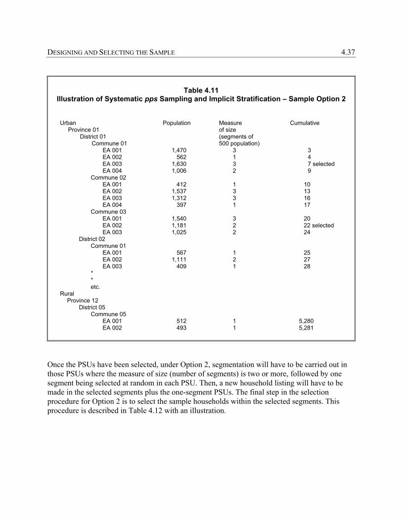
DESIGNING AND SELECTING THE SAMPLE 4.37

Table 4.11

Illustration of Systematic pps Sampling and Implicit Stratification – Sample Option 2

Urban Population Measure Cumulative Province 01 of size District 01 (segments of Commune 01 500 population) EA 001 1,470 3 3 EA 002 562 1 4 EA 003 1,630 3 7 selected EA 004 1,006 2 9 Commune 02 EA 001 412 1 10 EA 002 1,537 3 13 EA 003 1,312 3 16 EA 004 397 1 17 Commune 03 EA 001 1,540 3 20 EA 002 1,181 2 22 selected EA 003 1,025 2 24 District 02 Commune 01 EA 001 567 1 25 EA 002 1,111 2 27 EA 003 409 1 28 * * etc. Rural Province 12 District 05 Commune 05 EA 001 512 1 5,280 EA 002 493 1 5,281

Once the PSUs have been selected, under Option 2, segmentation will have to be carried out in those PSUs where the measure of size (number of segments) is two or more, followed by one segment being selected at random in each PSU. Then, a new household listing will have to be made in the selected segments plus the one-segment PSUs. The final step in the selection procedure for Option 2 is to select the sample households within the selected segments. This procedure is described in Table 4.12 with an illustration.

4.38 MULTIPLE INDICATOR CLUSTER SURVEY MANUAL

Table 4.12

Selecting the Households – Option 2 Suppose your standard segment size is 500 persons. Let your desired cluster size for the survey be designated as ñ households. 1. Calculate the average number of households per segment by dividing 500 by the average

household size in your country. Let this be sh. 2. Divide sh by ñ. This is your sampling interval, I, for selecting households within each sample

segment. (Note: If your standard segment size is other than 500, that value must be used.) Illustration: Suppose your average household size is 5.5. Then sh is 500/5.5, or 90.9. Suppose you want

your cluster size, ñ, to be 25. Divide 90.9 by 25 (1 decimal place) = 90.9/25, or 3.6. Then, select households in each segment at the rate of 1 in 3.6, starting with a random number between 01 and 36 (inserting the decimal after selecting the number).

PROCEDURES FOR SAMPLING WITH PPS – OPTION 3 If Option 3, the modified segment design described in this chapter, is used instead of Option 2, implicit stratification is done in the same way, although the measure of size is different. Under Option 3, if we suppose, as an example, that our segment size is going to be 20 households (on average), then the measure of size would be calculated by dividing the census count of households by 20, rounded to the nearest whole number. Note that under Option 3 the second column in Table 4.13 must be the number of households rather than population. You would calculate the sampling interval, I, by dividing the total cumulant – suppose it is 26,425 – by the desired number of PSUs, again, assume it to be 300. So, you would have 26,425/300 = 88.1. If the random start is chosen to be 19.4, the first two PSUs selected, as illustrated in Table 4.13, would be those corresponding to the smallest cumulants exceeding the values, 19.4 and 107.5 (88.1 + 19.4), respectively. They are EA 002 in commune 01 and EA 002 in commune 03 of province 01, district 01.

DESIGNING AND SELECTING THE SAMPLE 4.39

Table 4.13

Illustration of Systematic pps Sampling and Implicit Stratification – Sample Option 3

Urban Population Measure Cumulative Province 01 of size District 01 (segments of Commune 01 500 population) EA 001 290 14 14 EA 002 120 6 20 selected EA 003 325 16 36 EA 004 200 10 46 Commune 02 EA 001 81 4 50 EA 002 307 15 65 EA 003 261 13 78 EA 004 80 4 82 Commune 03 EA 001 308 15 97 EA 002 236 12 109 selected EA 003 205 10 119 * * * etc. Rural Province 12 District 05 Commune 05 EA 001 102 5 26,400 EA 002 99 5 26,405

Recall that, under Option 3, the measure of size is equivalent to the number of segments of pre-designated size that must be created (20 in our illustration). So, for the sample PSUs chosen, 6 segments of an approximate size of 20 households each must be formed in the first PSU and 12 in the second. Again, one of the segments would then be selected at random within each sample PSU, and all of the households within that segment would be interviewed for the survey, even if the actual number of households in the segment departs significantly from its expected size. Chapter 6 details the procedures for creating segments both for Option 2 and Option 3.

4.40 MULTIPLE INDICATOR CLUSTER SURVEY MANUAL

COUNTRY EXAMPLES FROM THE YEAR 2000 ROUND OF MICS

In the final section of this chapter we describe the sample designs that were used in three countries that participated in the year 2000 round of MICS. Each one illustrates a different aspect of the sampling points that have been discussed in this chapter. The examples are from Lebanon, Papua New Guinea and Angola. LEBANON We begin with Lebanon and provide a fairly detailed description in order to compare the sample design with the year 2000 MICS manual. In addition, we show how the weights were calculated to illustrate how this is done in a specific survey. Sample Plan

MICS was conducted by the Central Administration of Statistics. The principal measurement objectives of MICS were (1) to obtain the relevant, end-of-decade World Summit for Children indicators to profile the situation of women and children in Lebanon and (2) to provide these estimates at the national level and for five subnational areas (domains), which include the four largest muhafazas (governorates) plus the combination of Sud and Nabatieh. The sampling methodology for MICS in Lebanon was to select a probability sample of 1,625 households in each of the five domains using a stratified, clustered design. It was a two-stage selection process using the 1995-1996 Census of Buildings as the sampling frame. Altogether, 8,125 households were to be selected nationwide.

The first-stage clusters (that is, the primary sampling units – PSUs) were defined as ilots, and these were identical in concept and construction as census enumeration areas. They were selected with probability proportionate to their measures of size (or pps), the latter of which are the 1995-1996 counts of occupied dwellings from the Census of Buildings. A total of 65 ilots were selected in each domain, or 325 altogether. Ilots selected at the first stage were to be listed anew, that is, a fresh listing of households prepared in a field operation. Ilots that are very large were divided into geographical segments with one segment selected at random for listing. The new listing constituted the sampling frame for the second stage of selection. A fixed sample size of 25 households from the new listings was selected systematically in each sample ilot for the MICS interview. In a few of the sample ilots, that is, those that contained fewer than 25 households, all the households were surveyed for MICS. It was thought that non-response in the survey could be as high as 10 or 12 per cent, in which case the number of interviewed households would range from about 1,430 to 1,465 in each domain, or 7,150-7,325 nationwide.

DESIGNING AND SELECTING THE SAMPLE 4.41 Discussion of Sample Plan – MICS Philosophy It is significant to note that the sample plan described above is consistent with the overall MICS philosophy for sample design and implementation, according to the previous edition of the MICS manual. That edition, like the current one, promotes several features for sample design, all of which are faithfully followed in the plan undertaken by Lebanon’s Central Administration of Statistics. They include the following:

• Use of simple sampling methodology • Use of the latest census as the sample frame • Sampling in two stages • Use of probability techniques at every stage of selection • Use of clusters of moderate size • Use of an adequate sample size.

The sampling methodology is simple and straightforward, as opposed to complex; for this reason,

it was expected that non-sampling error would be kept to a minimum. The Census of Buildings in 1995-1996 was the appropriate frame to use because (1) it was the latest available and (2) maps were available, so that those ilots selected for MICS could be easily located and their internal boundaries identified. This cartographic aspect is also extremely convenient for the segmentation operation that was required for large ilots. The age of the frame meant that natural population movement and change could decrease the accuracy of the estimates, and for this reason, a new listing of households at the second stage was necessary to bring the frame up to date in the selected areas.

Strict probability selection methods were used at both stages. This helped ensure that the results

would be representative of the various target populations, including households, women of childbearing age and children in Lebanon. The cluster size of 25 households is moderate, which ensured that the sample design effect was not so large as to make the results unreliable for the important indicators.

The national sample size of 8,125 households was consistent with the recommendations in the 2000 edition of the MICS manual regarding this highly important survey parameter. As that manual pointed out, the sample size must be large enough to accomplish various measurement objectives. These include being able to measure key target indicators with a margin of error of 3-5 percentage points, depending upon the indicator. A second important objective was to be able to obtain reasonably reliable estimates of the indicators for the domains of interest (as mentioned in the summary, these included the four large governorates of Beyrouth, Mont Liban, Beqaa and Nord plus the combination, Sud/Nabatieh, as well as the national level).

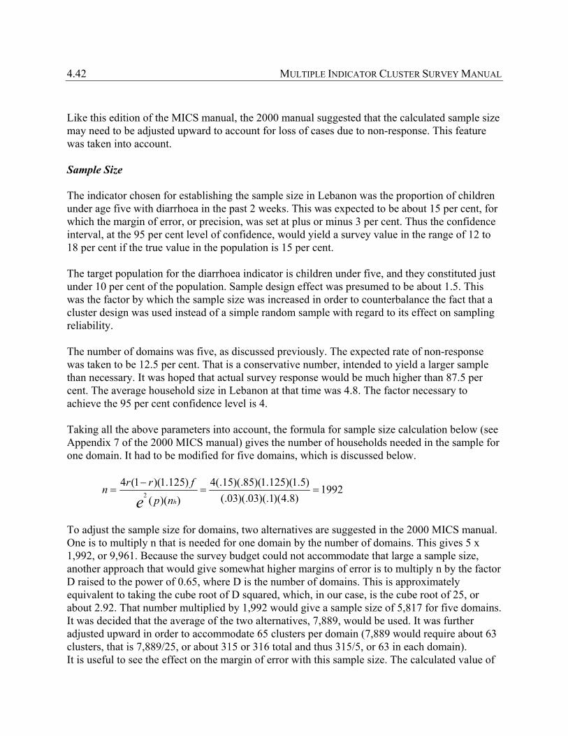
4.42 MULTIPLE INDICATOR CLUSTER SURVEY MANUAL Like this edition of the MICS manual, the 2000 manual suggested that the calculated sample size may need to be adjusted upward to account for loss of cases due to non-response. This feature was taken into account. Sample Size The indicator chosen for establishing the sample size in Lebanon was the proportion of children under age five with diarrhoea in the past 2 weeks. This was expected to be about 15 per cent, for which the margin of error, or precision, was set at plus or minus 3 per cent. Thus the confidence interval, at the 95 per cent level of confidence, would yield a survey value in the range of 12 to 18 per cent if the true value in the population is 15 per cent. The target population for the diarrhoea indicator is children under five, and they constituted just under 10 per cent of the population. Sample design effect was presumed to be about 1.5. This was the factor by which the sample size was increased in order to counterbalance the fact that a cluster design was used instead of a simple random sample with regard to its effect on sampling reliability.

The number of domains was five, as discussed previously. The expected rate of non-response was taken to be 12.5 per cent. That is a conservative number, intended to yield a larger sample than necessary. It was hoped that actual survey response would be much higher than 87.5 per cent. The average household size in Lebanon at that time was 4.8. The factor necessary to achieve the 95 per cent confidence level is 4.

Taking all the above parameters into account, the formula for sample size calculation below (see Appendix 7 of the 2000 MICS manual) gives the number of households needed in the sample for one domain. It had to be modified for five domains, which is discussed below.

1992)8.4)(1)(.03)(.03(.

)5.1)(125.1)(85)(.15(.4))((

)125.1)(1(42

==−

=hnp

frrne

To adjust the sample size for domains, two alternatives are suggested in the 2000 MICS manual. One is to multiply n that is needed for one domain by the number of domains. This gives 5 x 1,992, or 9,961. Because the survey budget could not accommodate that large a sample size, another approach that would give somewhat higher margins of error is to multiply n by the factor D raised to the power of 0.65, where D is the number of domains. This is approximately equivalent to taking the cube root of D squared, which, in our case, is the cube root of 25, or about 2.92. That number multiplied by 1,992 would give a sample size of 5,817 for five domains. It was decided that the average of the two alternatives, 7,889, would be used. It was further adjusted upward in order to accommodate 65 clusters per domain (7,889 would require about 63 clusters, that is 7,889/25, or about 315 or 316 total and thus 315/5, or 63 in each domain). It is useful to see the effect on the margin of error with this sample size. The calculated value of

DESIGNING AND SELECTING THE SAMPLE 4.43 n for diarrhoea is 1,992. Recall above that this would provide a margin of error of plus or minus 3 percentage points. The final sample size, however, is 8,125/5 or 1,625 per domain. Thus the margin of error is somewhat higher. The increase is calculated as the square root of the ratio of sample sizes, or the square root of 1,992/1,625, which is about 1.033. Thus the expected margin of error for this particular indicator at the governorate level would be about 3.3 percentage points, if the prevalence rate for diarrhoea was approximately 15 per cent.

Sample Allocation

The measurement objectives must be taken into account when deciding how to properly allocate

the sample. When national estimates take priority, the sample should be allocated proportionately among the various governorates. For example, if a governorate contains 35 per cent of the nation’s population, then 35 per cent of the sample would be selected in that governorate under the proportional allocation scheme. The problem with this approach, however, is that small governorates (say, one containing only 10 per cent of the population) would have too small a sample size to provide reliable estimates. The latter becomes a serious problem if the governorate level, as opposed to the national level, is the main priority.

The governorate level was in fact the main priority for the government and for

UNICEF/Lebanon. This is because programme planning and policy implementation projects to improve the situation of women and children must proceed at the local level. For that reason, estimates that were as reliable as possible were wanted for each of the governorates. To accomplish this, the sample had to be allocated equally among the governorates (the four large ones plus the southern combination).

Table 4.14 displays the allocation of the sample and the rest of its parameters by governorate.

Table 4.14 Sample Parameters – MICS 2000 in Lebanon

Muhafaza (governorate)

Sample size – number of households (hhs)

Sample size – number of clusters (ilots)

Cluster size – no. of sample hhs per cluster

Total number of frame units (occupied dwellings)

Sample interval to select ilots pps

Beyrouth 1,625 65 25 101,707 1 in 1,564.7 Mont Liban 1,625 65 25 356,517 1 in 5,484.9 Nord 1,625 65 25 150,018 1 in 2,308.0 Beqaa 1,625 65 25 97,638 1 in 1,502.1 Sud/Nabatieh 1,625 65 25 149,093 1 in 2,293.7 Lebanon total 8,125 325 25 854,973 -

4.44 MULTIPLE INDICATOR CLUSTER SURVEY MANUAL Implementation – Sample Selection Procedures

The first stage of selection was a systematic pps sample of census ilots, where the measure of size was the count of occupied dwellings. Prior to selection, the ilots were sorted by governorate and within governorate by caza (district), grand zone and ilot, the latter of which were geographically sequenced. This was all done using the seven-digit geographic identification code of the geographic database. In this way, the systematic selection that was carried out ensured implicit stratification of the sample for each of the domains, or governorates. Sixty-five ilots were thus selected in a computer operation for each domain.

To implement the second stage of selection, a current field listing of households was undertaken. Many of the sample ilots were very large and had to be segmented before conducting the listing. About 180 of the 325 ilots were segmented because they contain more than 150 households each, according to the 1995-1996 sampling frame.

Segmentation was carried out in accordance with Table 4.15.

Table 4.15

Number of Segments to Create

Number of households (according to frame)

Number of segments

Under 150 No segmentation 150-249 2 250-349 3 350-449 4 450-549 5 550-649 6 650-749 7 Etc. Etc.

Some of the sample ilots, about 12 of them, contained fewer than 25 households, according to the frame. For these ilots, no field listing was necessary. Instead, all households contained within the boundary of the ilot were interviewed for MICS, even if the number of such households at the time the MICS was conducted in 2000 was greater than 25.

For segmentation, Table 4.15 was used to figure how many segments to create. For example, if the frame showed that the sample ilot contained 580 households, six segments were created. Procedures about segment construction outlined in Chapter 6 of the 2000 edition of the MICS manual were followed. After segmentation, one segment was selected at random from each ilot that had been segmented.

For all ilots (under 150 households plus the selected segments for those greater than 150

DESIGNING AND SELECTING THE SAMPLE 4.45 households), another visit to the field was made in order to make a complete listing of the then-current households. Next, sampling of households was systematic within each ilot, or segment, at the rate of 1 in I, where I was the sample interval, equal to Ni ÷ η, where Ni was the actual number of households on the listing for the ith sample cluster, and η was 25, the desired cluster size. The value of the sampling interval, I, varied for each sample ilot or segment and it was calculated to one decimal place. Weighting and Estimation

To prepare the survey estimates, weighting had to be used because the sample was not self-weighting; in other words, the sample cases did not all have the same probability of selection. Weighting necessitated multiplying the raw sample data by the sample weight. Weights were variable by cluster since the weight for households in each cluster depends on the measure of size and the number of households obtained in the listing operation for that cluster. The weights are equal to the inverses of the probabilities of selection. The probability for the households, persons, children, women or any other target population group in a particular cluster is given by the following:

ihihh

ihih

sNMmP )25)(65(

= where

• Pih is the probability of selecting a household (or person) from the ith cluster

of the hth domain • 65 is the number of clusters in each domain • 25 is the cluster size • mih is the measure of size in the ith cluster of the hth domain, that is, the

number of occupied dwellings according to the sample frame • Nih is the number of households listed in the ith cluster of the hth domain • sih is the number of segments created in an ilot (the value of sih is 1 for ilots

that are not segmented) • Mh is the total measure of size in the hth domain, that is, the sum of the mih

values, or ∑ mih. Note that the value of Nih is the number of households listed in the cluster, which in non-segmented ilots is the entire ilot, while in segmented ilots it is the segmented part (see examples below).

As mentioned, the weight, Wih, is the inverse, or 1/ Pih .

4.46 MULTIPLE INDICATOR CLUSTER SURVEY MANUAL The Mh values are those in the fourth column of Table 4.14 for each of the domains. The product of 65 and 25 is 1,625. Weights, therefore, for households or persons for the five domains are as shown in Table 4.16.

Table 4.16

Survey Weights by Domain (for Ilots with 25 or more Households)

Governorate Weight Beyrouth (62.6Nisi)/mI Mont Liban (219.4NisI)/mI Nord (92.3Nisi)/mI Beqaa (60.1Nisi)/mI Sud/Nabatieh (91.7Nisi)/mI

EXAMPLE: Suppose in Beyrouth the measure of the size, mi, on the sample frame for the first sample cluster selected is 612. Thus it is segmented into six segments, which is the value of si. Suppose further that the number of households listed in the cluster is 110. Then the weight for all households and persons in sample for that cluster would be equal to (62.6)(110)(6)/(612), or 67.5. EXAMPLE: Suppose in Mont Liban the measure of the size, mi, on the sample frame for the first sample cluster selected is 106. Hence it is not segmented and the value of si is 1. Suppose further that the number of households listed in the cluster is 98. Then the weight for all households and persons in sample for that cluster would be equal to (219.4)(98)(1)/(106), or 202.8.

It was expected that it would be necessary to adjust the design weights discussed above by an additional factor to account for non-response. This was simply a matter of multiplying the weight, separately for each domain, by the ratio of sampled households to interviewed households. The product of the design weight and non-interview factor then becomes the final weight against which to multiply the raw sample counts to produce the estimates.

PAPUA NEW GUINEA MICS in Papua New Guinea was carried out by the National Statistics Office. Its design illustrates issues of sample frame updating and coverage as well as choosing between an existing survey sample (DHS) versus designing a new one. Weight calculation for the Papua New Guinea MICS is also informative. But it is somewhat similar to that of Lebanon, and therefore will not be presented here.

DESIGNING AND SELECTING THE SAMPLE 4.47 Summary of Sample Design Sampling was a two-stage selection process utilizing the 1991 Population Census, partially up-dated, as the sampling frame. The primary sampling units (PSUs) were defined as census enumeration areas or units (CUs). A total of 175 PSUs were selected with probability proportionate to their measures of size (pps), the latter of which were the 1991 household counts in rural areas and updated dwelling counts in urban areas. Census enumeration units selected at the first stage were listed anew; that is, a fresh listing of households was prepared in a field operation. The new listing constituted the sampling frame for the second stage of selection. A fixed sample size of 25 households from the listings was selected systematically in each sample CU for MICS. Altogether, 4,375 households was the targeted sample size.

The number of sample clusters was calculated as 175 by dividing 4,375 by 25. About 43 per cent were allocated to the urban stratum (75 clusters) and 57 per cent to the rural stratum (100 clusters). Before selection at the first stage, the frame was implicitly stratified by sorting the population census by urban and rural at the first level and by region, province, district, subdistrict and CUs at subsequent levels. Sample Frame Modification and DHS as an Alternative

The most recent census to use as a frame for sampling in the 2000 MICS in Papua New Guinea was the population census of 1991 – thus, it was 9 years old at the time. It was out of date to varying degrees in various areas of country, but primarily in urban areas, especially Port Moresby. At the time of the MICS, the National Statistics Office was also preparing to conduct the Year 2000 Population Census, and it intended to use the same census administrative units, CUs, that were used in the 1991 census. Those CUs were in the process of being updated through a new listing of households. At the time of the MICS, the updating had been confined to urban areas, which, for purposes of MICS, was the most important sector in terms of using the data as a sampling frame. The alternatives were to (1) postpone the MICS until the census update operation was completed in the rural areas or (2) use the old census as the sampling frame for rural areas and the updated one for urban areas. What is of key concern for any frame is to have measures of size – that is, counts of households to use in establishing the selection rate – that are fairly accurate. An important point to keep in mind, however, is that the measures of size do not need to be 100 per cent perfect, in order to use them validly for sample selection at the first stage. It was expected, therefore, that the rural CUs from the old census would have household counts that would differ from the situation in 2000 by only a few percentage points; thus, they were still fairly accurate. By contrast, the urban CUs were likely to be quite different, perhaps by factors of 2 or 3 or even greater, compared to 9 years earlier. This phenomenon occurs because, while relatively few people migrate from each rural CU, they all migrate to the same, comparatively few urban CUs. Thus it was much more important to have updated counts for the urban CUs than for the rural ones.

4.48 MULTIPLE INDICATOR CLUSTER SURVEY MANUAL It was consequently decided that, for MICS, two frames would be used for the sample design. For rural CUs, the 1991 Population Census was used as the frame. For urban CUs, the updated CU lists, with their revised count of dwellings that had been prepared for the Year 2000 Population Census were used.

Consideration was given to utilizing the Demographic and Health Survey (DHS) of 1996 as a frame alternative to the 1991 Population Census. This survey has similar objectives to MICS and the sample PSUs were updated in 1996. Thus, the rural PSUs were considerably more current in terms of measures of size than the 1991 census. However, the measurement objectives of DHS were to provide national level data, and this meant that the sample PSUs were distributed proportionately throughout the country. As such, the urban PSUs that were available from DHS were too few to use for MICS, where an important objective was to provide reliable data for the urban sector as a key estimation domain. Accordingly, the DHS was dropped from consideration.

Sample Coverage Certain, mostly interior, areas of Papua New Guinea are inaccessible except by helicopter. The Government felt that survey coverage of the population of these areas would be prohibitively expensive. Accordingly, the Government decided not to include inaccessible areas in MICS, even though it was recognized that the health status of women and children in such areas may be quite different than that of the rest of the country. To achieve a valid survey methodology it is important to eliminate the excluded areas from the sampling frame prior to sample selection. In this way, the sample that is chosen can still be a probability sample of the covered population, even though the latter is less than national in scope. The alternative of selecting the sample areas first and then substituting whenever an excluded area is chosen is a biased procedure statistically, and it was not used. Accordingly, a list of the inaccessible districts or subdistricts that were to be excluded from survey coverage was compiled and all CUs that make up those areas were eliminated from the sample frame. Sample Size and Allocation

The Government had hoped to conduct the MICS with a sample of about 2,500 households. The

2000 MICS manual urged countries to find a sample size that would enable them to measure their most important indicators with a margin of error of 3-5 percentage points (95 per cent level of confidence). At the national level, it was fully expected that 2,500 households would be sufficient to meet those requirements. However, the Government was also interested in having separate, reliable estimates for certain domains, that is, subnational areas that are important for policy planning. These are urban and rural areas, plus four regions: southern, northern, highlands and islands.

DESIGNING AND SELECTING THE SAMPLE 4.49

For the regional estimates, in particular, a sample size of 2,500 was thought to be insufficient, because there would only be, on average, about 625 households in each sample per region – not enough to yield very reliable estimates for key indicators. On a related point, the distribution of the population for the urban and rural sectors suggests that disproportionate sampling had to be used in order to obtain enough sample cases for the urban part. This is because only about 15 per cent of the population of Papua New Guinea reside in urban areas. If the sample were selected proportionally, therefore, less than 400 of the households would be urban, and in only 15 PSUs, both of which are too small of numbers to produce reliable results.

The above suggested two things: (1) oversampling should be used in the urban sector and (2) the

sample size should be increased, overall, to yield sufficient cases to provide reliable regional estimates.

The number of clusters – that is, the first-stage selection units (PSUs) – is also a factor that must

be taken into account for the domain estimates. With 100 PSUs, the average number for a given region would be only 25. This was too thin to provide adequate ‘spread’ of the sample at the regional level. There ought to be about 50 PSUs for each domain estimate, but the absolute minimum should not be less than 30. Accordingly, it was decided that the overall sample size be increased from 2,500 to 4,000 households. It was further decided to make an allowance of 10 per cent for non-response, thus increasing the sample size to about 4,375 households. The number of clusters was then also increased from 100 to 175 (4,375 ÷ 25).

Finally, it was decided that the urban stratum be oversampled by a factor of about 3, that is, an increase in the proportion of the overall sample that is urban from 15 per cent to 43 per cent. That would then yield about 1,875 households in 75 PSUs for the urban stratum and 2,500 households in 100 PSUs for the rural stratum. Oversampling in the urban areas was necessary in order to provide enough sample cases to provide reliable estimates. The disproportionate sample in the urban stratum, however, still left about 2,500 households in sample for the rural stratum, which was more than adequate for reliable figures. Implementation – Sample Selection Procedures In Papua New Guinea, the sample selection procedures were very similar to those in Lebanon – with one important difference. Thus we will only describe how they differed. Two options may be considered, according to the MICS manual (both editions), in deciding on a methodology to use in selecting households at the second (or third) stage. One is to carry out a new listing of households in the sample clusters and to select the households from the new listings. As mentioned in the manual, this is the preferred approach for the MICS, both because it is slightly more reliable and somewhat less complicated than the alternative. The alternative, however, is an approach that has the advantage of avoiding the expense of listing, which can be considerable, and that is the main reason it is suggested in the manual as a suitable option. That option entails constructing geographic segments of approximately equal size in each sample cluster (CUs for Papua New Guinea), selecting one at random and

4.50 MULTIPLE INDICATOR CLUSTER SURVEY MANUAL interviewing all the households within the chosen segment for MICS. As implied above, however, the alternative, though valid, is not as reliable as the listing approach because the households in the sample are ‘clustered’ together and the sample design effect is therefore somewhat greater. Secondly, segmentation is more complicated than listing and may therefore introduce greater non-sampling error, especially if the staff persons are not well trained in the proper use of maps, including segment sketching. The National Statistics Office decided to opt for the preferred approach – listing instead of segmentation. ANGOLA The Multiple Indicator Cluster Survey was implemented by the Instituto Nacional de Estatistica in Angola. The sample design for the MICS in that country illustrates survey implementation done in two phases, months apart, as well as associated issues of population coverage, frame deficiencies and presentation of results to users. Summary of Sample Design The principal measurement objectives of MICS were (1) to obtain the relevant, end-of-decade World Summit for Children indicators to profile the situation of women and children in Angola and (2) to provide these estimates at both the national level and for three ecological zones (domains) – litoral, planalto and interior. The sampling methodology for MICS 2000 in Angola made use of probability selection procedures to choose about 6,660 households in a stratified, clustered design. The survey was administered in a two-phase operation, with the first phase utilizing a sample frame developed for the 2000-2001 Survey of Income and Expenditures (Inquerito sobre Despesas e Receitas, or IDR). The second phase, conducted approximately 2-3 months later, was carried out in the balance of the MICS survey universe, that is, in territory that was excluded from the IDR. The latter phase was delayed because sampling frame materials first had to be developed for it. Sample Selection Sample selection was a two-stage selection process in urban areas and three stages in rural areas. The first-stage units (that is, the primary sampling units – PSUs) are defined as ‘seccaos censitarias’ in urban areas and they consist of geographically defined segments – typically municipal blocks – that contain an average of about 100 households. In rural areas, the clusters are communes, and the secondary units are villages. Thus, the MICS clusters themselves are the first-stage units in urban areas, but second-stage units in rural areas.

DESIGNING AND SELECTING THE SAMPLE 4.51 The clusters were selected in the so-called ‘covered’ areas of the country. These are defined as government-controlled, accessible areas of the country and consist, generally, of provincial and/or municipal capitals, plus some rural areas. Sample coverage was carried out by first removing from the sampling frames those areas that were to be excluded due to problems of internal security and/or access, including areas that were purportedly mined. In addition, internally displaced persons who were living in camps were not covered by the main survey, although there was a plan for sampling and interviewing them as a separate operation. Sample selection of first-stage units was done with probability proportionate to their measures of size (or pps). The measures of size, m.o.s., were then-current counts of houses or other dwellings in urban areas and current estimates of the rural population in rural areas. The counts were obtained from actual field canvassing, while the estimates were taken from local information provided at the provincial level. A total of 408 clusters were selected – 300 from the phase-one IDR frame and 108 from the residual, phase-two frame. Sampling procedures differed for the two phases. In phase one, the MICS clusters were a systematic subset of those already selected for IDR. These clusters had already been listed anew, that is, a fresh listing of households was prepared in a field operation for the IDR. This listing constituted the sampling frame for the last stage of selection. A systematic selection of 15 households was selected in each of the 300 MICS clusters of phase one, independent of the households that were chosen for the IDR, in order to avoid overlap between the two survey interviews. Twenty households per cluster were chosen in the 108 phase- two clusters.23 In phase two, the sample frame had to be developed in the same way as it was developed for the IDR, except that it was extended to those MICS provinces and other areas that were not covered by IDR. Thus, the phase-two frame constituted the source for the selection of the 108 clusters. They were selected using probability proportionate to size. Selected clusters were then listed in the field, so that the second-stage selection of 20 households per cluster could be carried out. This was done using systematic selection. The sample of 6,660 households was distributed proportionately among the three ecological zones or domains. Each of the domains was large enough, in terms of population, so that reliable results could be provided at the domain level with the use of proportionate allocation of the sample. It was thought that non-response in the survey would be about 10 per cent, in which case the number of households actually interviewed for the survey was expected to be closer to 6,000.

23 The cluster sizes differ between phase one and phase two because 20 households per cluster was the recommended number for MICS (see the 2000 edition of the MICS manual), but 15 households was more convenient operationally to select from the IDR frame.

4.52 MULTIPLE INDICATOR CLUSTER SURVEY MANUAL It was not possible to estimate accurately the percentage of the population to be covered by the survey, since current demographic data were not available. It was thought, however, that perhaps 10 per cent of the population resided in camps for internally displaced persons and another 15-25 per cent resided in the inaccessible areas. Thus, it was estimated that about 65-75 per cent national population coverage would be attained by the MICS (see next section). Sample Frame and Coverage

Perfect sampling frames are rarely encountered in practice anywhere, but satisfying the three criteria of completeness, accuracy and currency was especially difficult in Angola. There are several reasons. One is that the usual frame used for national sample surveys is the latest census, which, in the case of Angola, would be the 1970 population census, and that was too out of date for consideration. Thus, other, more recent frames, had to be used – ones that were likely to be somewhat inferior to a current census frame (see further discussion below).

Second, as already mentioned, mined areas were excluded from coverage, as were camps for internally displaced persons and other inaccessible areas. As a result, the criterion of completeness was violated, and to an unknown degree, although it was speculated that national coverage would be about 65-75 per cent, as mentioned above. Third, the available frames suffered from inaccuracies of unknown magnitude, especially in the rural areas where the quality of the population estimates (used to establish the probabilities of selection at the first stage) were thought to be widely variable province-to-province.

The implications for MICS 2000 in Angola were that the survey results would be biased and to an unknown degree, if the results had been presented as though they represent the entire country. This is because ‘representativeness’ cannot be statistically justified for the subpopulations excluded from coverage – subpopulations that are likely to have somewhat different characteristics from those that were included. Another important implication is that estimates of the size of the national population could not be made from MICS, because of lack of coverage of the excluded subpopulations.

Nevertheless, valid and useful results were obtained from the covered population of the MICS, by using careful probability methods in selecting the sample households from the frames that were used, even though these frames were somewhat imperfect. In terms of survey coverage, the frame that was developed by the Instituto Nacional de Estatistica for the IDR was excellent as far as it went. It was a valid and defensible source to use for phase one. The problem with it was that it covered only seven provinces and, within those provinces, usually urban territory only. This is why it was necessary to develop another frame for phase two – to cover the additional 11 provinces, plus as much rural area as could be deemed accessible for surveying.

An important lesson on release of data to the public is learned from the Angola MICS. Release of the survey results in reports should always be handled by stating, as precisely and clearly as

DESIGNING AND SELECTING THE SAMPLE 4.53 possible, the definition of the actual population covered by the survey. In the case of Angola, it was important to inform users that the MICS presented scientifically defensible results for approximately 65-75 per cent of the population of Angola, but did not represent persons living outside government-controlled areas, those residing near certain excluded areas that are mined and internally displaced persons residing in camps.