WWRC-83-08

DESIGN RAINFALL DISTRIBUTIONSFOR THE

STATE OF WYOMING

Patrick T. TyrrellVictor R. Hasfurther August, 1983

Department of Civil EngineeringCollege of EngineeringUniversity of Wyoming

Research Project TechnicalCompletion Report (A-036-WYO)Agreement No. 14-34-0001-2154

Prepared for:U. S. Department of the Interior

The research on which this report is based was financedin part by the U. S. Department of the Interior, as authorizedby the Water Research and Development Act of 1978 (P.L. 95-467).

Contents of this publication do not necessarily reflectthe views and policies of the U.S. Department of the Interior,nor does mention of trade names or commercial productsconstitute their endorsement or recommendation for use by theU. S. Government.

Wyoming Water Research CenterUniversity of Wyoming

Laramie, Wyoming

TABLE OF CONTENTS

Page

INTRODUCTION . . . . . . . . . . . 1

REVIEW OF PREVIOUS WORK . . . . . . . . 2

METHODOLOGY . . . . . . . . . . . 4

Accumulation of Rainfall Data . . . . . 4

Description of Study Area . . . . . . 7

Analysis of Storm Parameters . . . . . 7

Construction of Design Curves . . . . . 10

Comparison of Storm Design Methods . . . . 13

DESIGN STORM RESULTS . . . . . . . . 13

Statistical Analysis . . . . . . . 13

Presentation and Use of Design Curves . . . 15

RESULTS OF DESIGN STORM COMPARISONS . . . . . 21

General Information . . . . . . . 21

Model Parameters . . . . . . . . 23

Design Hyetographs . . . . . . . . 24

DISCUSSION OF RESULTS . . . . . . . . 32

SUMMARY AND CONCLUSIONS . . . . . . . . 34

Summary . . . . . . . . . . . 34

Conclusions . . . . . . . . . . 34

REFERENCES . . . . . . . . . . . 36

LIST OF TABLES

Table Page

I. Precipitation Stations Providing Data forStudy . . . . . . . . . . 5

II. Description of Digital Computer Models Used inDesign Storm Comparisons . . . . . 14

III. Results of Selected Statistical Analysis ofRainfall Characteristics . . . . . 16

IV. Recommended Time Intervals and CorrespondingPercent Time Increments for ObtainingRainfall Versus Time Data from DesignCurves . . . . . . . . . 20

V. Loss Parameters Used with Rainfall RunoffModels for Storm Comparison . . . . 24

VI. Comparative Hyetographs for 10 year, 2-hourThunderstorm . . . . . . . . 25

VII. Comparative Hyetographs for 10 year, 6-hourGeneral Storm . . . . . . . . 26

VIII. Comparative Hyetographs for 10 year, 24-hourGeneral Storm . . . . . . . . 27

IX. Runoff Characteristics for 10 year, 2-hourThunderstorm . . . . . . . . 30

X. Runoff Charateristics for 10 year, 6-hourGeneral Storm . . . . . . . . 31

XI. Runoff Characteristics for 10 year, 24-hourGeneral Storm . . . . . . . . 31

LIST OF FIGURES

Page

Fig. 1 Map of the State of Wyoming showing the

major surface water drainage basins.

Station numbers refer to Table I . . . . 8

Fig. 2 Dimensionless design mass curves for

thunderstorms . . . . . . . . . 11

Fig. 3 Dimensionless design mass curves for general

storms. . . . . . . . . . . 18

Fig. 4 Variation in peak intensity with storm duration . 33

INTRODUCTION

The design of hydraulic structures for use in ungaged drainage basins

requires some estimate of flood flows and their frequency of occurrence.

Because no historical streamflow data exist for these drainages, floods are

estimated either by regional frequency analysis or, with the help of

digital computers, by parametric rainfall-runoff event simulation.

Computer models dealing with rainfall-runoff event simulation are

commonly used today by engineers and hydrologists. These models are used

to predict flood hydrographs given an input rainfall volume, distributed

over time in some manner, and certain geomorphic basin parameters.

Studies exist in the literature documenting the effects of time

distribution of rainfall on runoff hydrographs. The reader is referred to

works by Wei and Larson (1971), Yen and Chow (1980), and Shanholtz and

Dickerson (1964) as examples. Because this relationship between the time

distribution of rainfall and hydrograph characteristics exists, the separ-

ate study of storm rainfall is essential for accurate flood prediction

regardless of other variables that also influence the runoff process.

Additionally, methods of constructing design storms are available and in

wide use, but they are general in nature and assume storms occur with the

same temporal distribution across much of the country. Because of the

drastic climatic differences between the areas encompassed by existing

procedures, it was felt their design curves are not likely to be

representative of the actual time distribution of storms in semi-arid

regions such as Wyoming. It was, therefore, decided to develop a new

2

design storm construction procedure applicable to the State of Wyoming

based on observed storm rainfall in Wyoming. This new design storm

methodology is the topic addressed herein.

REVIEW OF PREVIOUS WORK

Relatively few precipitation studies made to date deal with the

temporal distribution of rainfall as used by hydrologists and engineers in

parametric flood prediction.

The Soil Conservation Service (SCS) method (1973) presents two

temporal rainfall distribution curves for runoff prediction. For studies

in Hawaii, Alaska, and the coastal side of the Sierra Nevada and Cascade

mountain ranges, the Type I and IA curves are used. The Type II curve is

applied in the remaining part of the United States, Puerto Rico, and the

Virgin Islands. These curves are based on generalized rainfall depth-

duration curves obtained from published data of the U.S. Weather Bureau

(National Oceanic and Atmospheric Administration). All design storms

developed with this method, regardless of duration, are based on the 24-

hour volume for a given frequency and location.

The Bureau of Reclamation method (1977) is developed in two parts, one

for the United States east of the 105° meridian and the other for areas

west of the 105° meridian. The procedure requires arranging hourly

rainfall increments in a specified sequence depending on the duration and

type of storm (thunderstorm or general storm). Maximum 6-hour point

rainfall values are used in designing general storms, and maximum 1-hour

point rainfall values are used in designing thunderstorms.

3

The U.S. Weather Bureau procedure (1961) uses depth-duration-frequency

(DDF) curves in design storm construction. In this method rainfall

intensities are obtained from the DDF curves for a given frequency and

duration at a certain locality. These intensities are then rearranged

arbitrarily to form a storm pattern.

Kerr, et al., (1974) present a method of hyetograph construction for

the State of Pennsylvania. Cumulative dimensionless rainfall versus time

graphs used by the method are derived from historical rainfall data. The

curves allow the user much flexibility because, rather than define a single

storm sequence, they bracket a range of possible storm patterns. Picking

the time distribution of a design storm is up to the user, providing he

stays within the limits of the bracketing curves and the minimum and

maximum intensities given.

Huff (1967) presents a procedure derived from heavy storms observed in

Illinois. His distribution patterns are based on the time quartile in

which the majority of rain occurs for a given storm. For each quartile

storm type, frequency values are given so that the user knows the return

period of his design storm.

A method described in Keifer and Chu (1957) uses intensity-duration-

frequency curves for hyetograph design at a given location. In general,

the proposed storm pattern is fit to exponential growth and decay curves

with the most intense part of the storm defined by a parameter termed the

"advanceness ratio." This method was developed in Chicago for urban sewer

design but can easily be used in other areas of the country where adequate

rainfall records are available.

4

Frederick, et al. (1981) developed annual maximum precipitation events

for different durations. The largest precipitation amounts for the

selected durations which coincide with a given duration event are selected.

The events are stratified according to magnitude and ratios of shorter to

longer duration precipitation totals are formed. Accumulated probabilities

of this ratio are suggested as a tool to estimate precipitation increments

necessary in the synthesis of precipitation mass curves. By analyzing the

relative timing of the shorter duration event within the longer duration

event, a characteristic time distribution can be developed.

METHODOLOGY

Accumulation of Rainfall Data

The study of time distribution of rainfall requires historic data

recorded as nearly continuously as possible. Because continuously recorded

rainfall data were not available in the quantities needed for this study,

discrete data were used. Hourly measurements from the National Oceanic and

Atmospheric Administration (NOAA) publications (1948-1979) provided the

data base for the study of general storms while the five-minute incremental

precipitation data available in Rankl and Barker (1977) were used in

thunderstorm analysis. Table I describes the precipitation stations used

from both sources.

The definition of a storm had to be established before usable

information could be obtained from the data. In this report, the criteria

used for defining a storm are as follows:

General Storm - preceded and followed by at least two hours of

zero rainfall

5

TABLE I.

PRECIPITATION STATIONS PROVIDING DATA FOR STUDY___________________________________________________________________Reference Location Name or Major Drainage Recording

Number Number Basin Source Interval__1 Casper WSO AP North Platte NOAA1 Hourly2 Cheyenne WSFO AP North Platte NOAA Hourly3 Douglas Aviation North Platte NOAA HOURLY4 Encampment North Platte NOAA Hourly5 Jelm North Platte NOAA Hourly6 Laramie 2 WSW North Platte NOAA Hourly7 Medicine Bow North Platte NOAA Hourly8 Oregon Trail Crossing North Platte NOAA Hourly9 Pathfinder Dam North Platte NOAA Hourly

10 Phillips North Platte NOAA Hourly11 Pine Bluffs North Platte NOAA Hourly12 Rawlins FAA AP North Platte NOAA Hourly13 Saratoga 4 N North Platte NOAA Hourly14 Seminoe Dam North Platte NOAA Hourly15 Shirley Basin Station North Platte NOAA Hourly16 Torrington 1 S North Platte NOAA Hourly17 Wheatland 4 N North Platte NOAA Hourly18 Buffalo Powder NOAA Hourly19 Douglas 17 NE Powder NOAA Hourly20 Dull Center Powder NOAA Hourly21 Gillette 18 SW Powder NOAA Hourly22 Hat Creek 14 N Powder NOAA Hourly23 Lance Creek Powder NOAA Hourly24 Moorcroft Powder NOAA Hourly25 Mule Creek Powder NOAA Hourly26 Newcastle Powder NOAA Hourly27 Osage Powder NOAA Hourly28 Pine Tree 9 NE Powder NOAA Hourly29 Powder River Powder NOAA Hourly30 Recluse Powder NOAA Hourly31 Sheridan WSO AP Powder NOAA Hourly32 Story Powder NOAA Hourly33 Boysen Dam Big Horn NOAA Hourly34 Lander WSO AP Big Horn NOAA Hourly35 Meteetse 1 ESE Big Horn NOAA Hourly36 Powell Field Station Big Horn NOAA Hourly37 Riverton Big Horn NOAA Hourly38 Tensleep 4 NE Big Horn NOAA Hourly39 Thermopolis Big Horn NOAA Hourly40 Thermopolis 25 WNW Big Horn NOAA Hourly41 Worland Big Horn NOAA Hourly42 Big Piney Green NOAA Hourly43 Mountain View Green NOAA Hourly

6

TABLE I. continued

PRECIPITATION STATIONS PROVIDING DATA FOR STUDY___________________________________________________________________Reference Location Name or Major Drainage Recording

Number Number Basin Source Interval__44 Mud Springs Green NOAA Hourly45 Rock Springs FAA AP Green NOAA Hourly46 Lake Yellowstone Yellowstone NOAA Hourly47 Jackson Snake NOAA Hourly48 Moran 5 WNW Snake NOAA Hourly49 Evanston 1 E Bear NOAA Hourly50 06631150 North Platte USGS2 5-minutely51 06634910 North Platte USGS 5-minutely52 06634950 North Platte USGS 5-minutely53 06644840 North Platte USGS 5-minutely54 06648720 North Platte USGS 5-minutely55 06648780 North Platte USGS 5-minutely56 06312910 Powder USGS 5-minutely57 06312920 Powder USGS 5-minutely58 06313050 Powder USGS 5-minutely59 06313180 Powder USGS 5-minutely60 06316480 Powder USGS 5-minutely61 06382200 Powder USGS 5-minutely62 06233360 Big Horn USGS 5-minutely63 06238760 Big Horn USGS 5-minutely64 06238780 Big Horn USGS 5-minutely65 06256670 Big Horn USGS 5-minutely66 06267260 Big Horn USGS 5-minutely67 06267270 Big Horn USGS 5-minutely68 06274190 Big Horn USGS 5-minutely

______________________________________________________________________1 NOAA (1948-1979)2 Rankl and Barker (1977)======================================================================

7

- at least four hours in duration

- at least one. half (0.5) inch in volume

Thunderstorm - preceded and followed by at least one hour of

zero rainfall

- at least twenty minutes and at most four hours

in duration

- at least one-half (0.5) inch in volume

These criteria are arbitrary but consistent with similar criteria put

forth by Huff (1967), Ward (1973), and Croft and Marston (1950). Minimum

duration requirements were used to make sure the time distribution of any

storm was described by at least four data points. In all, 531 general

storms and 72 thunderstorms were examined.

The period of record represented by the data at most stations covers

the years 1969-1979, though the lack of definable storms at some stations

required data from as far back as 1948. Because the development of design

storms inherently assumes future rainfall events will occur with the same

distribution as past events, the use of data from stations with variable

periods of record is acceptable.

Description of Study Areas

The State of Wyoming was divided into its major surface water drainage

basins for this study. This was done to see if differences in storm

rainfall characteristics exist between basins. Figure 1 shows the entire

State of Wyoming divided into these major drainages.

Analysis of Storm Parameters

Determining if differences in storm rainfall characteristics exist

between basins requires statistical analysis of certain storm parameters.

9

Definitions of parameters used in describing storm rainfall follow:

Storm Duration - the amount of elapsed time, in hours, from the

beginning to the end of a storm.

Storm Volume - the total amount of rainfall measured during a

storm, in inches.

Storm Intensity - the average rainfall rate during a storm, in inches

per hour, calculated by dividing a storm's volume

by its duration.

Percent Time to Peak Intensity - that amount of time, expressed as a

percent of total storm duration, from the beginning

of a storm to the period of most intense rainfall.

Pattern Index - the area beneath a dimensionless cumulative rainfall

versus time curve, expressed as a decimal or as a

percent.

Pattern Index and Percent Time to Peak Intensity were the parameters

used for determining if differences in the time distribution of rainfall

exist between basins. This determination was made using a one-way analysis

of variance technique for samples of unequal size. The procedure,

described in Miller and Freund (1977), tests for differences in the

population means for the populations from which the samples were taken.

Such tests indicate if significant differences in parameter values exist

between all the major drainages. If differences existed, the state would

have to be divided accordingly before design storms could be constructed.

If no differences existed, the state as a whole could be analyzed with the

resulting design storms applicable statewide.

10

Construction of Design Curves

All the observed dimensionless mass rainfall curves are superimposed

on one graph to create a family of "probable" storm patterns. Such an

approach to design storm development is described in Kerr, et al. (1974).

The method's most attractive feature is its flexibility, allowing the user

his choice of three given design hyetographs, as well as the freedom to

construct his own hyetograph, within limits. Such flexibility is desirable

when, for example, a person is designing a structure based on peak flowrate

in one instance and on runoff volume in another. The use of several curves

can allow maximization of either peak flowrate or runoff volume for a

given storm volume. A single design curve does not have this ability.

Figure 2 is a set of design curves. All of the storms used in the

development: of this set of curves are non-dimensionalized and plotted on

one graph of percent rainfall versus percent time. The bold vertical lines

at each ten percent time increment represent the range of all storm data

used. In the center of the plot is the mean curve. The curve is fit

through the points representing the average cumulative percent rainfall at

each ten percent time increment. It should be noted that the mean curve

does not describe the average observed storm, rather it shows average

accumulated rainfall with time based on all storms used. Also drawn on the

plot: are ten percent and 90 percent limit curves. The ten percent limit

curve represents, at a given percentage of storm duration, that value

above which ten percent of the storms had accumulated more precipitation.

Similarly, ten percent of the storms had each accumulated less than the

value described by the 90 percent limit line at a given percentage of storm

duration. It is not correct to assume that ten percent of the storms were

12

totally above the ten percent limit line or totally below the 90 percent

limit line. The use of ten percent as the cutoff when defining the upper

and lower limit lines is arbitrary but reasonable. Using a smaller cutoff

percentage resulting in a broader set of enveloping limit curves would be

too general to accurately predict probable storm patterns. A larger cutoff

value would result in a narrower envelope and a loss in flexibility of the

method.

Under the assumption that future rainfall events will have the same

time distribution as past events, these limit curves are the boundaries of

a region of probable storm sequences. The user of the curves has the

freedom to use either limit curve, or the mean curve, when choosing a

design storm. In fact, he may pick his own storm sequence as long as he

stays between the limit curves at all times and adheres to the maximum and

minimum slope guidelines printed at the top of Figure 2. These guidelines

are constructed in a manner similar to the limit curves in that for each

ten percent time interval they represent intensities exceeded by ten

percent of the storms (the steeper line) as well as intensities exceeded in

90 percent of the storms (the less steep line). In using these intensity

guidelines, the designer cannot create a storm with an intensity greater

than the value defined by the steep line or less than that defined by the

shallow line for the appropriate ten percent increment of storm duration.

The number accompanying each of these lines at the top of Figure 2 is the

slope of that line.

Designing storms in this manner makes the utmost use of historical

rainfall patterns while allowing the user flexibility in choosing the time

13

distribution which will provide the critical peak flowrate or runoff volume

for his purpose.

Comparison of Storm Design Methods

The creation of new storm patterns for use in a particular region is

logically accompanied by a comparison of the results of using the new

method with results obtained using established design storm techniques.

Such a comparison will prove the need for the new region-specific design

curves if the existing general methods do not produce similar runoff

characteristics when applied to a given event.

The different storm designs are compared by inputting them to four

different rainfall-runoff simulation models and examining the runoff

hydrographs produced. Thunderstorm and general storm runoff are simulated

with each model. For each model and storm type the infiltration parameters

are held constant so that any differences noted in outflow hydrograph

characteristics can be attributed to differences in the input hyetographs.

The models used are described in Table II. In addition to the design storm

construction method presented in this paper, techniques given by the U.S.

Soil Conservation Service (1973) and the U.S. Bureau of Reclamation (1977)

are used for comparative purposes. These last two methods have already

been described in the review of previous work.

DESIGN STORM RESULTS

Statistical Analysis

Examination of the linear regression and analysis of variance (ANOVA)

tests performed on the rainfall data leads to the following conclusions:

1. A difference in the time distribution of thunderstorm rainfall

TABLE II

DESCRIPTION OF DIGITAL COMPUTER MODELS USED IN DESIGN STORM COMPARISONS

=======================================================================================================Method of estimating Method of constructing

Model Citation infiltration outflow hydrograph_______________________________________________________________________________________________________SCS Triagular U.S. Soil Conser- Uses a "minimum infiltration Relates incremental excessHydrograph vation Service rate" and runoff curve num- precipitation to incremental

(1972). ber based on soil type. runoff with a hydrographthat is triangular in shape.

HEC-1 U.S. Army Corps Uses an exponentially decay- Derives outflow hydrographof Engineers ing function that depends on from either (1) unitgraph(1973). rainfall intensity and ante- input by either, or (2) Clark

cedent losses. (1945) synthetic unitgraph.

HYMO Williams and Hann Similar to SCS method Uses dimensionless unitgraph(1973). U.S. De- above; uses curve number and (described by exponentialpartment of Agri- minimum infiltration rate. expressions relating flowrateculture. to time) and a "dimensionless

shape parameter."

USGS Dawdy, David R., Uses the Philip (1954) var- Performs finite differenceJohn C. Shaake, Jr.,iation of the Green-Ampt solution of kinematic waveand William M. (1911) equation. Method in- equation for each channel andAlley (1978). cludes soil-moisture account- overland flow segment in drain-U.S. Geological ing between storms. age basin.Survey.

========================================================================================================

15

compared to general storm rainfall exists for the entire State

of Wyoming.

2. The time distribution of both thunderstorms and general storms

is not dependent upon the drainage basin in which the storms

occur.

3. No relationship exists between time distribution character-

istics and duration of general storms or thunderstorms.

Inferred by 1 and 2 above is the need for only one set of general

storm design curves and one set of thunderstorm design curves for use

statewide. Conclusion 3 says that design storms of varying duration, i.e.,

1-, 2-, or 3-hour thunderstorms or 6-, 12-, or 24-hour general storms, can

all be handled with the same set of design curves. Table III lists the

results of selected important linear regression and ANOVA tests used in

drawing these conclusions. The rest of the statistical analysis results

can be found in Tyrrell (1982).

Probably the most outstanding characteristic of the storms analyzed is

their individual diversity. This same finding is corroborated in the paper

by Kerr, et al. (1974) for storms in Pennsylvania. It is precisely because

of this diversity that the use of an enveloping set of curves is preferred

to the use of a single storm pattern when attempting to predict runoff.

Presentation and Use of Design Curves

Figures 2 and 3 are the design curves for thunderstorms and general

storms, respectively, constructed according to the procedures outlined

previously. Figure 2 is to be used when the duration of the design storm

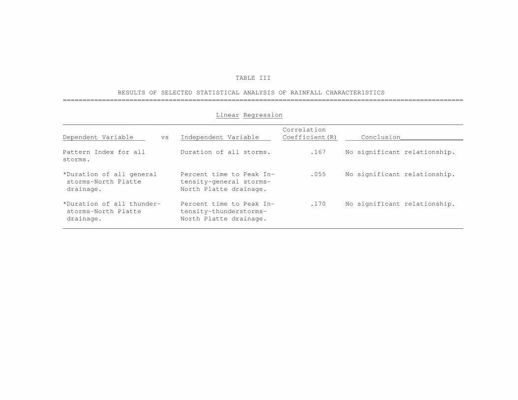
TABLE III

RESULTS OF SELECTED STATISTICAL ANALYSIS OF RAINFALL CHARACTERISTICS======================================================================================================

Linear Regression______________________________________________________________________________________________________

CorrelationDependent Variable vs Independent Variable Coefficient(R) Conclusion________________

Pattern Index for all Duration of all storms. .167 No significant relationship.storms.

*Duration of all general Percent time to Peak In- .055 No significant relationship.storms-North Platte tensity-general storms-drainage. North Platte drainage.

*Duration of all thunder- Percent time to Peak In- .170 No significant relationship.storms-North Platte tensity-thunderstorms-drainage. North Platte drainage.

______________________________________________________________________________________________________

TABLE III, continued

RESULTS OF SELECTED STATISTICAL ANALYSIS OF RAINFALL CHARACTERISTICS======================================================================================================

Analysis of Variance______________________________________________________________________________________________________

Null Hypothesis (Ho) F Statistic ConclusionData F.05 F.10 _______________________________________

Pattern Index values for general 1.22 2.44 1.99 Do not reject Ho; conclude no differencestorms are equal for all five in Pattern Index due to drainage basinmajor drainages. location.

Pattern Index values for thunder- .79 3.14 2.38 Do not reject Ho; conclude no differencestorms are equal for three in Pattern Index due to drainage basinmajor drainages. location.

*Pattern Index values are equal for 24.65 3.91 2.74 Reject Ho; conclude some difference inthunderstorms and general storms- Pattern Index due to type of storm.North Platte River drainage._______________________________________________________________________________________________________*Results from the North Platte drainage data analysis are presented as an example. Results from theother basins are similar.

=======================================================================================================

19

of interest is less than four hours. Figure 3 is used for events four

hours long or longer.

Following is a list of steps involved in using the design curves:

1. Select the storm type to be simulated at a certain location;

for example, the 10-year, 6-hour event at Buffalo, Wyoming.

Consult some source of rainfall frequency data, such as the

Rainfall Frequency Atlas by Miller, et al. (1973), to find the

volume of rain expected for this event.

2. Select the appropriate set of design curves. For the example

above, the general storm curves (Figure 3) are applicable

because the duration is longer than four hours.

3. Select one curve from the plot, either the ten percent or ninety

percent limit curve, the mean curve, or some non-standard curve.

When choosing a non-standard curve, the user must remember to

stay on or between the limit curves at all times. Also, the

steepness (intensity) of a curve in any ten percent time

interval is dictated by the "maximum and minimum allowable

intensities" shown at the top of the design curves. A non-

standard curve must not be more steep than the steeper of these

two lines (the maximum intensity line), or less steep than the

line with smaller slope (the minimum intensity line) in any

given ten percent interval of storm time. Examples of non-

standard time distributions are given in following sections of

this report.

4. Using the curve from Step 3, select the percent rainfall values

that correspond to the percent time values. A maximum time

20

interval length of one hour is suggested. Table IV recommends

percent time increments to be used for storms of varying duration.

TABLE IV

RECOMMENDED TIME INTERVALS AND CORRESPONDING PERCENTTIME INCREMENTS FOR OBTAINING RAINFALL VERSUS

TIME DATA FROM DESIGN CURVES

=====================================================================Interval as a

Storm Recommended Number of Percent ofDuration Time Interval Intervals Storm Duration30 minute 5 minute 6 16.67%1 hour 10 minute 6 16.67%2 hour 15 minute 8 12.50%3 hour 15 minute 12 8.33%6 hour 30 minute 12 8.33%

12 hour 1 hour 12 8.33%24 hour 1 hour 24 4.17%

=====================================================================

5. Organize the data obtained in Step 4 into the form required

by whatever model is being use; i.e., rainfall either as

actual depth or a percent of storm value, sequences either

cumulative or incremental.

6. Run the model with infiltration and geomorphic parameters as

required.

It is recommended that the user run several simulations with different

hyetographs to determine the critical runoff volume or peak flowrate. The

suite of design curves used probably will include both limit curves, the

mean curve, and several curves chosen arbitrarily by the user.

21

A parameter not included in this study is the areal distribution of

rainfall. Therefore, the user of the method presented here is obliged to

reduce point rainfall values when working with large drainage basins.

Methods of reducing point rainfall with increasing drainage basin area are

presented in Design of Small Dams (U.S. Bureau of Reclamation, 1977) and in

the Rainfall Frequency Atlas (Miller, et al., 1973). These reductions are

necessary because of the tendency of point rainfall values to overestimate

actual areal precipitation on large areas.

Because this new design method depicts "probable" events, rather than

extreme events (i.e., ultra-high-intensity bursts or long periods of very

intense rain), it should not be used when designing for runoff due to

"probable maximum" rainfall. Existing methods for probable maximum design

(as in Small Dams) should be consulted for those cases.

RESULTS OF DESIGN STORM COMPARISONS

General Information

The purpose of this section is to compare the use of differing design

storms in parametric flood prediction. Computer models used are HEC-1,

HYMO, HYDRO (SCS Triangular Hydrograph method), and USGS (USGS distributed

routing model). The reader is referred back to Table II for descriptions

of these models. Design storms recommended by the U.S. Bureau of

Reclamation (1977) and the U.S. Soil Conservation Service (1973) are used

in the comparison.

The procedure followed in the comparison was to input differing

design storms to a model, while leaving all geomorphic and loss parameters

unchanged, and examine differences in the simulated outflow hydrograph peak

22

and volume. Variations thus found are attributable to variations in the

input hyetograph.

Some problems were encountered in the use of existing design storms.

For example, the SCS method, rather than using a rainfall volume based on a

certain duration for a given frequency, uses the 24-hour amount for

designing storms of all durations. This practice results in slightly

different storm volumes than those found in the Miller, et al. (1973),

publication for varying durations. Despite this anomaly, the SCS

hyetograph was used without a volume correction. Thus, a valid method-by-

method comparison is ensured. The Bureau of Reclamation (BUREC) method

also involves an odd twist basing its storm volumes on fractions and

multiples of the 6-hour value for a given frequency. Modern practice has

corrected this deficiency by allowing the use of volumes expected for

various durations, not a manipulation of the 6-hour amount, while retaining

the recommended time sequence. The BUREC method also typically calls for

basing designs on runoff from a 3-hour thunderstorm and an 18-hour general

storm. Because there exists no 18-hour duration precipitation data, no

storms of this length were used in comparison. Also, a 2-hour thunderstorm

was deemed most representative of short duration events (thus, the 3-hour

event was not used).

Storms selected for the comparisons were 2, 6 and 24 hours in

duration. The 2-hour event is considered a thunderstorm; the other two are

general storms. A small drainage in the Powder River Basin provided the

geomorphic data for the simulations. Storm volumes (U.S. Weather Bureau,

1961) for the duration's listed above (with a 1O-year return period) at this

location are:

23

2-hour - 1.60"

6-hour - 2.00"

24-hour - 2.75"

while the geomorphic parameters for the basin are:

Drainage Area - 0.83 mi²

Water Course Length - 1.38 mi.

Elevation Difference - 125 feet

Model Parameters

Table V lists the loss parameters used with each model. The values

of these parameters were not changed at any time. "NA" means the particular

model does not use that parameter. It should be emphasized that values of

loss parameters for the HYDRO, HYMO, USGS, and HEC-1 models are not

calibrated values; they are values presented by Haie (1980) as

representative for the Powder River Basin of Wyoming. A requirement of the

USGS program, however, forced optimization of PSP. An optimization range

of 4.0 - 6.0 was, therefore, used. The resulting small fluctuations in

the value of PSP were not felt to harm the objectivity of the testing

procedure. Because of the soil moisture accounting capability of the USGS

model, antecedent rainfall and evaporation data was needed to "prepare" the

soil prior to the occurrence of the storm event. Arbitrary, but

consistent, amounts of .03 inches of daily precipitation and .01 inches of

daily evaporation were applied for thirty days leading up to the simulated

storm.

Because all the results presented herein were obtained using non-

calibrated infiltration parameters, they are useful for comparison purposes

only.

24

TABLE V

LOSS PARAMETERS USED WITH RAINFALL RUNOFF MODELS

FOR STORM COMPARISON

==========================================================================Mon. Infil-

Curve tration RateModel Number (in/hr) STRKR1 DRTKR1 RTIOL1 ERAIN1 TC1 R1

HYDRO 72 .15 NA NA NA NA NA NA

HYMO 72 .15 NA NA NA NA NA NA

HEC-1 NA NA .80 .20 2.75 .70 1.0 5.0

PSP* KSAT* RGI* BMSN* EVC* RR* DRN/(24·KSAT)*

USGS 5.0 0.10 10.0 5.0 0.7 0.9 0.5

==========================================================================*For definition of parameters refer to dawdy, et al. (1978).1The reader is referred to the HEC-1 users manual (U.S. Army Corps ofEngineers, 1973) for definitions of these infiltration parameters.

Design Hyetographs

Tables VI, VII, and VIII present the design hyetographs used for each

duration given as cumulative rainfall amounts. The "WYO" distribution

sequences come from the curves presented in Figures 2 and 3. Those

WYO storms designated A, B, C. etc., correspond to non-standard curves

arbitrarily picked by the authors. These hyetographs can be

graphically constructed by plotting the tabular values on a percent

rainfall versus percent time basis, if the reader wishes to compare them

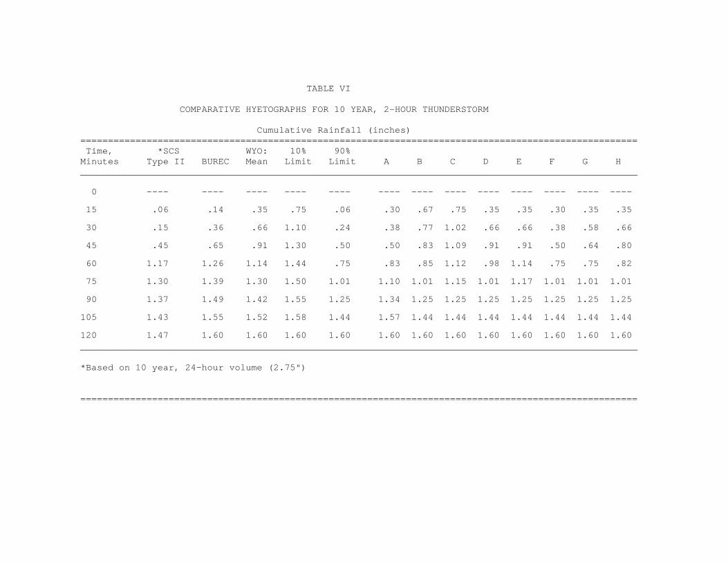
TABLE VI

COMPARATIVE HYETOGRAPHS FOR 10 YEAR, 2-HOUR THUNDERSTORM

Cumulative Rainfall (inches)=====================================================================================================Time, *SCS WYO: 10% 90%

Minutes Type II BUREC Mean Limit Limit A B C D E F G H_____________________________________________________________________________________________________

0 ---- ---- ---- ---- ---- ---- ---- ---- ---- ---- ---- ---- ----

15 .06 .14 .35 .75 .06 .30 .67 .75 .35 .35 .30 .35 .35

30 .15 .36 .66 1.10 .24 .38 .77 1.02 .66 .66 .38 .58 .66

45 .45 .65 .91 1.30 .50 .50 .83 1.09 .91 .91 .50 .64 .80

60 1.17 1.26 1.14 1.44 .75 .83 .85 1.12 .98 1.14 .75 .75 .82

75 1.30 1.39 1.30 1.50 1.01 1.10 1.01 1.15 1.01 1.17 1.01 1.01 1.01

90 1.37 1.49 1.42 1.55 1.25 1.34 1.25 1.25 1.25 1.25 1.25 1.25 1.25

105 1.43 1.55 1.52 1.58 1.44 1.57 1.44 1.44 1.44 1.44 1.44 1.44 1.44

120 1.47 1.60 1.60 1.60 1.60 1.60 1.60 1.60 1.60 1.60 1.60 1.60 1.60_____________________________________________________________________________________________________

*Based on 10 year, 24-hour volume (2.75")

=====================================================================================================

TABLE VII

COMPARATIVE HYETOGRAPHS FOR 10 YEAR, 6-HOUR GENERAL STORM

Cumulative Rainfall (inches)=====================================================================================================Time, *SCS WYO: 10% 90%Minutes Type II BUREC Mean Limit Limit C G_____________________________________________________________________________________________________

0 ---- ---- ---- ---- ---- ---- ----

30 .04 .18 .34 .04 .04 .34

60 .10 .14 .36 .68 .10 .10 .68

90 .17 .56 1.00 .22 .36 .84

120 .24 .32 .74 1.24 .34 .68 .88

150 .41 .92 1.44 .50 1.00 .94

180 1.41 .54 1.12 1.60 .68 1.34 .98

210 1.62 1.30 1.72 .90 1.68 1.04

240 1.72 1.50 1.46 1.82 1.12 1.82 1.12

170 1.80 1.64 1.88 1.34 1.88 1.34

300 1.86 1.82 1.76 1.94 1.56 1.94 1.56

330 1.92 1.90 1.98 1.78 1.98 1.78

360 1.96 2.00 2.00 2.00 2.00 2.00 2.00_____________________________________________________________________________________________________

*Based on 10 year, 24-hour volume (2.75")

=====================================================================================================

TABLE VIII

COMPARATIVE HYETOGRAPHS FOR 10 YEAR, 24-HOUR GENERAL STORMCumulative Rainfall (inches)

=====================================================================================================Time, SCS WYO: 10% 90%hours Type II BUREC Mean Limit Limit A B C D E F G H_____________________________________________________________________________________________________

0 --- --- --- --- --- ---- ---- ---- ---- ---- ---- ---- ----

1 .03 .05 .11 .22 .03 .03 .03 .03 .03 .22 .22 .22 .22

2 .06 .14 .25 .47 .06 .06 .06 .06 .06 .47 .47 .47 .47

3 .09 .22 .36 .72 .08 .08 .08 .08 .08 .72 .72 .72 .61

4 .13 .33 .50 .94 .14 .14 .14 .14 .14 .94 .94 .94 .63

5 .17 .44 .66 1.16 .22 .22 .22 .25 .22 1.16 1.16 1.10 .66

6 .22 .55 .77 1.38 .30 .30 .30 .50 .30 1.38 1.38 1.16 .72

7 .28 .66 .91 1.54 .39 .39 .39 .72 .39 1.54 1.54 1.18 .74

8 .34 .80 1.02 1.71 .47 .47 .58 .94 .47 1.71 1.60 1.21 .77

9 .41 .96 1.16 1.84 .58 .58 .80 1.18 .58 1.84 1.65 1.27 .83

10 .51 1.71 1.27 1.98 .69 .74 1.02 1.38 .69 1.93 1.68 1.29 .85

11 .65 1.95 1.40 2.09 .80 .96 1.27 1.62 .80 1.98 1.71 1.32 .88

12 1.82 2.09 1.54 2.20 .94 1.18 1.49 1.84 .94 2.01 1.73 1.35 .94

13 2.13 2.15 1.65 2.28 1.07 1.40 1.71 2.06 1.18 2.04 1.76 1.38 1.07

14 2.26 2.20 1.79 2.37 1.24 1.62 1.93 2.31 1.40 2.06 1.79 1.43 1.24

15 2.34 2.25 1.90 2.45 1.38 1.84 2.15 2.45 1.62 2.09 1.84 1.49 1.38

16 2.42 2.31 2.01 2.50 1.54 2.09 2.37 2.50 1.84 2.12 1.87 1.54 1.54

TABLE VIII continued

COMPARATIVE HYETOGRAPHS FOR 10 YEAR, 24-HOUR GENERAL STORM

Cumulative Rainfall (inches)=====================================================================================================Time, SCS WYO: 10% 90%hours Type II BUREC Mean Limit Limit A B C D E F G H_____________________________________________________________________________________________________

17 2.48 2.37 2.12 2.53 1.68 2.28 2.53 2.53 2.06 2.15 1.90 1.68 1.68

18 2.54 2.42 2.26 2.59 1.84 2.50 2.59 2.59 2.26 2.17 1.90 1.84 1.84

19 2.58 2.47 2.34 2.64 2.01 2.64 2.64 2.64 2.48 2.20 2.01 2.01 2.01

20 2.62 2.53 2.42 2.67 2.15 2.67 2.67 2.67 2.64 2.20 2.15 2.15 2.15

21 2.66 2.59 2.53 2.70 2.28 2.70 2.70 2.70 2.70 2.28 2.28 2.28 2.28

22 2.70 2.64 2.61 2.72 2.45 2.72 2.72 2.72 2.72 2.45 2.45 2.45 2.45

23 2.72 2.69 2.67 2.72 2.59 2.72 2.72 2.72 2.72 2.59 2.59 2.59 2.59

24 2.75 2.75 2.75 2.75 2.75 2.75 2.75 2.75 2.75 2.75 2.75 2.75 2.75_____________________________________________________________________________________________________

=====================================================================================================

29

visually with the standard 10%, 90% and mean WYO curves. The reader can

see that, due to the discrepancy previously described, the SCS storm

volumes do not quite equal the volumes given by the BUREC and WYO storms in

Tables VI and VII.

The 6-hour event was the last of the three to be evaluated. Results

from the earlier runs for the 2- and 24-hour events were used to indicate

which of the lettered (A, B, C, etc.) WYO curves would probably give the

largest peak runoff flowrate. As a result, the 6-hour event was run with

only the "C" and "G" arbitrary curves used in addition to the mean, ten

percent limit, and 90 percent limit curves.

Tables IX, X, and XI present the results of the model runs for the 2-

hour, 6-hour and 24-hour events, respectively. Generally, results from

HEC-1, HYMO, and HYDRO simulations show that for longer events the WYO

curves produce less runoff (Peak and Volume) than the other methods, while

for shorter events the WYO curves produce greater runoff. Results from

USGS model runs differed from the other models* results by predicting, for

all three storm durations, smaller runoff peaks and volumes due to the WYO

design curves when compared to established procedures. Because of these

results, it is suggested that current methods may lead to consistent over-

design of hydraulic structures, at least when long (durations of 6 or more

hours) events are stated as part of the design criteria. Also, the ability

of any one of the group of WYO curves to produce greater runoff than the

others is dependent upon the model used. These results are further

detailed in the following section.

30

TABLE IX

RUNOFF CHARACTERISTICS FOR 10 YEAR 2-HOUR THUNDERSTORM========================================================================

MODEL:HYDRO HYMO HEC-1 USGS____

Peak Vol. Peak Vol. Peak Vol. Peak Vol.Design Storm (cfs) (in.) (cfs)(in.) (cfs)(in.) (cfs) (in.)_________________________________________________________________________

SCS Type II 47.8 .098 11.7 .036 38 .39 41.1 .162

BUREC 65.3 .137 17.3 .053 36 .38 40.2 .162

WYO-Mean 61.7 .139 12.9 .040 28 .31 16.0 .094

10% Limit 61.8 .123 19.9 .061 42 .45 33.2 .146

90% Limit 76.1 .135 30.7 .100 29 .32 20.6 .107

-A 79.6 .134 41.7 .133 31 .34 24.7 .118

-B 75.3 .133 30.9 .100 32 .39 23.1 .124

-C 62.2 .124 17.2 .064 34 .42 22.2 .138

-D 72.6 .132 30.7 .100 29 .35 19.3 .105

-E 62.5 .130 21.0 0.80 28 .34 18.0 .102

-F 76.1 .135 30.7 .100 27 .31 19.9 .105

-G 76.1 .135 30.7 .100 27 .32 19.2 .103

-H 76.7 .134 30.7 .100 28 .33 18.9 .103

========================================================================

31

TABLE X

RUNOFF CHARACTERISTICS FOR 10 YEAR 6-HOUR GENERAL STORM========================================================================

MODEL:HYDRO HYMO HEC-1 USGS____

Peak Vol. Peak Vol. Peak Vol. Peak Vol.Design Storm (cfs) (in.) (cfs)(in.) (cfs)(in.) (cfs) (in.)_________________________________________________________________________

SCS Type II 85.3 .175 42.7 .143 36 .38 47.1 .184

BUREC 81.6 .251 37.6 .205 20 .23 19.4 .116

WYO-Mean 52.8 .275 18.9 .094 2 .03 6.7 .065

10% Limit 50.5 .208 26.9 .103 11 .14 8.5 .075

90% Limit 83.6 .287 54.8 .261 10 .12 12.4 .085

-C 89.1 .221 49.4 .164 18 .22 16.7 .101

-G 83.6 .226 55.8 .261 10 .16 10.5 .082

========================================================================

TABLE XI

RUNOFF CHARACTERISTICS FOR 10 YEAR 24-HOUR THUNDERSTORM========================================================================

MODEL:HYDRO HYMO HEC-1 USGS____

Peak Vol. Peak Vol. Peak Vol. Peak Vol.Design Storm (cfs) (in.) (cfs)(in.) (cfs)(in.) (cfs) (in.)=========================================================================

SCS Type II 138.6 .346 57.9 .285 30 .34 43.1 .189

BUREC 95.5 .268 45.9 .221 14 .16 14.4 .103

WYO-Mean 0 0 0 0 0 0 1.49 .043

10% Limit 24.3 .107 14.7 .091 0 0 2.22 .051

90% Limit 8.0 .085 6.5 .074 0 0 2.88 .056

-A 50.9 .428 35.5 .352 0 0 5.16 .072

-B 37.6 .400 29.0 .327 0 0 4.91 .070

-C 50.9 .384 36.6 .319 0 0 5.18 .069

-D 37.6 .412 27.7 .343 0 0 4.94 .071

-E 24.3 .134 1.7 .005 0 0 2.22 .057

-F 24.3 .120 14.7 .099 0 0 2.31 .057

-G 8.1 .075 6.1 .063 0 0 2.82 .056

-H 8.1 .085 6.5 .074 0 0 2.88 .056

========================================================================

32

DISCUSSION OF RESULTS

The most significant difference between the WYO design storm

methodology and those developed by the Soil Conservation Service and Bureau

of Reclamation is the use of totally dimensionless curves. By non-

dimensionalizing the time axis, the average intensities of designed storms

is decreased as the storm durations are increased. For example, if two

general storms of the same volume but differing durations, say 6 hours and

12 hours, were distributed over time according to the mean curve of Figure

3, the 12-hour storm would have half the intensity of the 6-hour event at

any point along the curve. This explains why the WYO curves tend to

produce smaller runoff peaks than the other methods for long events, and

larger peaks for short events. Such a change in intensity with duration

may seem inappropriate at first, but analysis of one hundred runoff-

producing storms recorded by Ranki and Barker (1977) shows that, while

there is not a good linear relationship (R = 53%), the peak intensity of a

storm appears to decrease with increasing storm length. Figure 4 suggests

this graphically. It, therefore, seems reasonable for the WYU storm design

technique to make long storms generally less intense than short storms.

Lower rainfall intensity, as obtained from the WYO curves, is the

reason zero runoff is predicted in some instances for the 24-hour event.

For example, referring to Table XI, no runoff is produced using the WYO

mean curve with the HYDRO and HYMO models. One will notice that, for

general storms, the WYO mean curve is almost a 45° line indicating an

almost constant intensity storm. For the 24-hour event, this constant

intensity (.11 in/hour) is less than the minimum infiltration loss of .15

in/hour. Thus, no runoff occurs. Similarly, the HEC-1 model produces zero

33

runoff in several instances. Because shorter storms do produce runoff

according to HEC-1, the reason for zero predicted runoff in the longer

storms obviously also involves low rainfall intensity and associated

infiltration losses.

It is interesting to note that choosing a WYO curve for producing peak

runoff flowrate or volume depends on the computer model to be used. For

instance, referring to Table IX, the WYO 90 percent limit curve produces

more runoff (peak and volume) than the ten percent limit curve when HYDRO

and HYMO are used. When HEC-1 is used, the ten percent limit curve yields

the greatest runoff peak and volume. The user of these curves is,

therefore, warned not to assume that a peak-producing hyetograph for one

34

model will perform similarly with a different simulation scheme. Always

test several curves for their peak-producing ability when changing models,

or when changing storm durations with the same model.

SUMMARY AND CONCLUSIONS

Summary

Parametric flood prediction on ungaged basins in Wyoming requires the

use of temporal storm patterns that realistically represent anticipated

local rainfall events. Because methods of hyetograph construction

currently in use are very general in application, this requirement is not

met. Therefore, a design storm methodology based on analysis of time

distribution characteristics of 603 observed storms in Wyoming is

presented. The "WYO" method of storm design uses not one, but several mass

rainfall curves, allowing flexibility of use and maximization of runoff

from a given storm volume.

Comparisons were made between the WYO method and design storms

recommended by the U.S. Soil Conservation Service and U.S. Bureau of

Reclamation using HEC-1, HYMO, HYDRO (Triangular Hydrograph), and USGS

Distributed Routing rainfall-runoff models.

Conclusions

1. The time distribution of both thunderstorms and general storms

is not dependent upon the drainage basin in which the storms

occur.

2. The most outstanding characteristic of the storms analyzed is

their individual diversity. No relationship exists between time

35

distribution characteristics and duration of general storms

or thunderstorms. However, a difference in the time distribution

of thunderstorm rainfall, compared to general storm rainfall,

exists.

3. One set of thunderstorm design curves and one set of general

storm design curves can be used to create design hyetographs

for the entire State of Wyoming.

4. The "WYO" design storm methodology should not be used to

design for "probable maximum" type events because the most

intense rainfall values have been neglected by the defini-

tion of ten percent and 90 percent limit curves.

5. Simulation of runoff peak and volume using WYO design curves

is sensitive to storm duration and choice of model.

6. WYO curves typically predict greater runoff peaks than Soil

Conservation Service or Bureau of Reclamation synthetic hyeto-

graphs for short duration events, and less runoff for long

duration events, according to HEC-1, HYMO, and HYDRO model

results.

7. WYO curves consistently produce less runoff than Soil Conserva-

tion Service or Bureau of Reclamation synthetic hyetographs

when the USGS Distributed Routing model is used.

REFERENCES

Clark, C. 0., 1945, Storage and the Unit Hydrograph, Am. Soc. Civil

Engineers Trans., V. 110, pp. 1419-1488.

Croft, A. R., and Richard B. Marston, 1950, Summer Rainfall Character-

istics in Northern Utah, Trans. Am. Geophysical Union, Vol. 31,No. 1, pp. 83-95.

Dawdy, David R., John C. Schaake, Jr., and William M. Alley, 1978,

Distributed Routing Rainfall-Runoff Model, U. S. GeologicalSurvey, Water-Resources Investigations 78-90, 146 p.

Frederick, Ralph H., John F. Miller, Francis P. Richards and Richard W.

W. Schwerdt, 1981, Interduration Precipitation Relations ForStorms - Western United States, NOAA Technical Report NWS 27,U. S. Department of commerce, 195 pp.

Green, W. H. and G. A. Ampt, 1911, Studies on Soil Physics; I, Flow

of Air and Water Through Soils: Jour. Agr. Research, V. 4,p. 1-24.

Haan, Charles T., and B. J. Barfield, 1978, Hydrology and Sedimentol-

ogy of Surface Mined Lands, Lexington, Kentucky: University ofKentucky.

Haie, Nairn, 1980, Rainfall-Runoff Models for Ephemeral Streams in the

Eastern Powder River Basin of Wyoming, M. S. Thesis, Universityof Wyoming, 56 pp.

Huff, F. A., 1967, Time Distribution of Rainfall in Heavy Storms,

Water Resources Research 3(4):1007-1019.

Keifer, Clint J., and Henry Hsien Chu, 1957, Synthetic Storm Pattern

for Drainage Design, Journal of the Hydraulics Division, ASCE,Vol. 83, No. HY4.

Kerr, R. L., T. M. Rachford, B. M. Reich, B. H. Lee, and K. H.

Plummer, 1974, Time Distribution of Storm Rainfall in Pennsyl-vania, Pennsylvania State University, Institute for Research onLand and Water Resources, 34 pp.

Miller, Irwin, and John E. Freund, 1977, Probability and Statistics

for Engineers, Second Ed. Prentice-Hall, Inc., Englewood Cliffs,New Jersey.

Miller, J. F., R. H. Frederick and R. J. Tracey, Precipitation-Frequency

Atlas of the Western United States, Vol. II, Wyoming. NOAAAtlas 2. U. S. Dept. of Commerce, Silver Spring MD, 1973

37

National Oceanic and Atmospheric Administration (NOAA), 1948-1979,

Hourly Precipitation Data for Wyoming, National Climatic CenterAsheville, North Carolina.

Philip, J. R., 1954, An Infiltration Equation with Physical Signifi-

cance: Soil Sci. Soc. Am. Proc., V. 77, p. 153-157.

Ranki, J. G., and D. S. Barker, 1977, Rainfall and Runoff Data from

Small Basins in Wyoming, Wyoming Water Placing Program ReportNo. 17, 195 pp.

Shanholtz, V. 0., and W. H. Dickerson, 1964, Influence of Selected

Rainfall Characteristics on Runoff Volume, West Virginia Uni-versity Agricultural Experiment Station, Bulletin 4971.

Tyrrell, Patrick T., 1982,. Development of Design Rainfall Distribu-

tion for the State of Wyoming, M. S. Thesis, University of Wyo-ming, 71 pp.

U. S. Army Corps of Engineers, 1973, HEC-1 Flood Hydrograph Package,

Users and Programmers° Manuals, HEC Program 723-X6-L2010.

U. S. Bureau of Reclamation, 1977, Design of Small Dams, U. S.

Dept. of the Interior, Washington, D.C.: U. S. GovernmentPrinting Office.

U. S. Soil Conservation Service, 1973, A Method for Estimating Volume

and Rate of Runoff in Small Watersheds, SC-TP-149, Department ofAgriculture.

U. S. Weather Bureau, 1961, Rainfall-Frequency Atlas of the United

States for Durations from 30 Minutes to 24 Hours and ReturnPeriods from 1 to 100 Years. Tech. Paper 40, 115 pp.

U. S. Weather Bureau, 1978, Use of DDF Curves in Storm Construction,

In Hydrology and Sedimentology of Surface Mined Lands, Haanand Barfield (1978), pp. 49-52.

Ward, Tim, 1973, Quantification of Rainfall Characteristics, Unpub-

lished. CWRR-DRI, University of Nevada System, Reno, Nevada.

Wei, Tseng C., and C. L. Larson, 1971, Effects of Areal and Time

Distribution of Rainfall on Small Watershed Runoff Hydrographs,Minnesota Univ., Minneapolis, Water Resources Research Center,Bulletin No. 30, 130 pp.

Williams, J. R., and R. W. Hann, 1973, HYMO: Problem-Oriented Com-

puter Language for Hydrologic Modeling, U. S. Department ofAgriculture,Agriculture Research Service.

Yen, Ben Chie, and Ven Te Chow, 1980, Design Hyetographs for Small

Drainage Structures, Journal of the Hydraulics Division, ASCE,Vol. 106.,No. HY6.