Kano State Point Rainfall Seasonal Arima Model Prediction in R

Kano State Point Rainfall Seasonal Arima Model

Prediction in R

I.M. SANNI, H.A. AHMED, U.A. ABUBAKAR & S.A. ABDULLAHI Ahmadu Bello University Zaria, Nigeria

ABSTRACT Point rainfall field data from 1983 to 2017 of Kano State located in

the Chad Basin was obtained from Nigeria Meteorology Agency, for prediction

using Seasonal Auto Regressive Integrated Moving Average (SARIMA) Model in

R programming. Exploratory data analysis, time series decomposition, plots of

Auto Correlation factor (ACF) and Partial Auto Correlation factor (PACF), fitting

the model, diagnostic test were applied to obtain the prediction model parameters

p,d,q,P,D,Q followed with prediction and accuracy test checked. It was revealed

that there was a seasonal cycle of appreciable rainfall that begins in April with in-

creases in trend to August (the threshold month), then decline to March. Presence

of a slowly increasing rainfall trend was observed in the time series. The rainfall

data has a mean higher than the median, which shows a positively skewed series

and a heavy tailed distribution of kurtosis greater than 3. The best SARIMA Model

parameters of the order (6,0,2,0,1,3,12) was selected at minimum AIC of 8.707182.

The prediction shows a insignificant decrease in rainfall amount from 2018 to 2030

with Mean Error (ME) of -8.65, Root Mean Square Error (RMSE) of 28.27 and

Mean Absolute Error (MAE) of 18.88.

Keywords: SARIMA, diagnostic check, accuracy check, predictive model parame-

ters Introduction

Rain is needed as a source of fresh water, which is essential for the survival of hu-

mans, plants and animals. Rain fills aquifers, lakes and rivers, sustain agricultural

processes and maintaining the lives of living organisms. The process of evapora-

tion exhausts fresh water sources, necessitating rain to replace the lost water. The

flow of minerals within the soil, and from the land to the sea, is mediated by rain.

The collection of rainfall data in a sequential order over a time period (rainfall time

series data) can be used to make a reasonable deduction for water resources man-

agement (‘why do we need rain?’, retrieved 12 August, 2019).

Time series analysis comprises methods for analyzing time series data in

order to extract meaningful statistics and other characteristics inherent in the data,

to develop appropriate models that describe future values based on previously ob-

served values. Owing to the prominence of time series many intelligent time series

models have been developed to improve the accuracy and efficiency of time series

forecasting (Adhikari and Agrawal, 2014). One of the most widely used and recog-

nized statistical forecasting time series models is the Autoregressive Integrated

Proceedings on Big Data Analytics & Innovation (Peer-Reviewed),

Volume 4, 2019, pp. 24-35

K�� S� P�� R�� S�� A�� M�� P�� R

25

Moving Average (ARIMA) model, with simplicity as well as the associated Box–

Jenkins methodology for optimal model construction (Khandelwal, et. al. 2015).

Although the method can handle data with a trend, it does not support time series

with a seasonal component. For seasonal time series forecasting, Box and Jenkins

(Box & Jenkins, 1976) proposed a quite successful extension to ARIMA model

that supports the direct modeling of univariate time series data containing trends

and seasonality called SARIMA (Seasonal Autoregressive Integrated Moving Av-

erage) (Priyaranjan, 2017).

SARIMA model prediction of daily point rainfall from 1983 to 2017 was

carried out in R programming environment. The aim was to develop an appropriate

model that could describe the future values of rainfall in the basin based on previ-

ously observed records. The daily rainfall data was converted into monthly maxi-

mum rainfall, divided into training dataset from1983–2012 used to develop the

predictive model and testing dataset from 2013–2017 used in the validation of the

formulated model. Building the model, the outlines steps were follows according to

Aishwarya (2018):

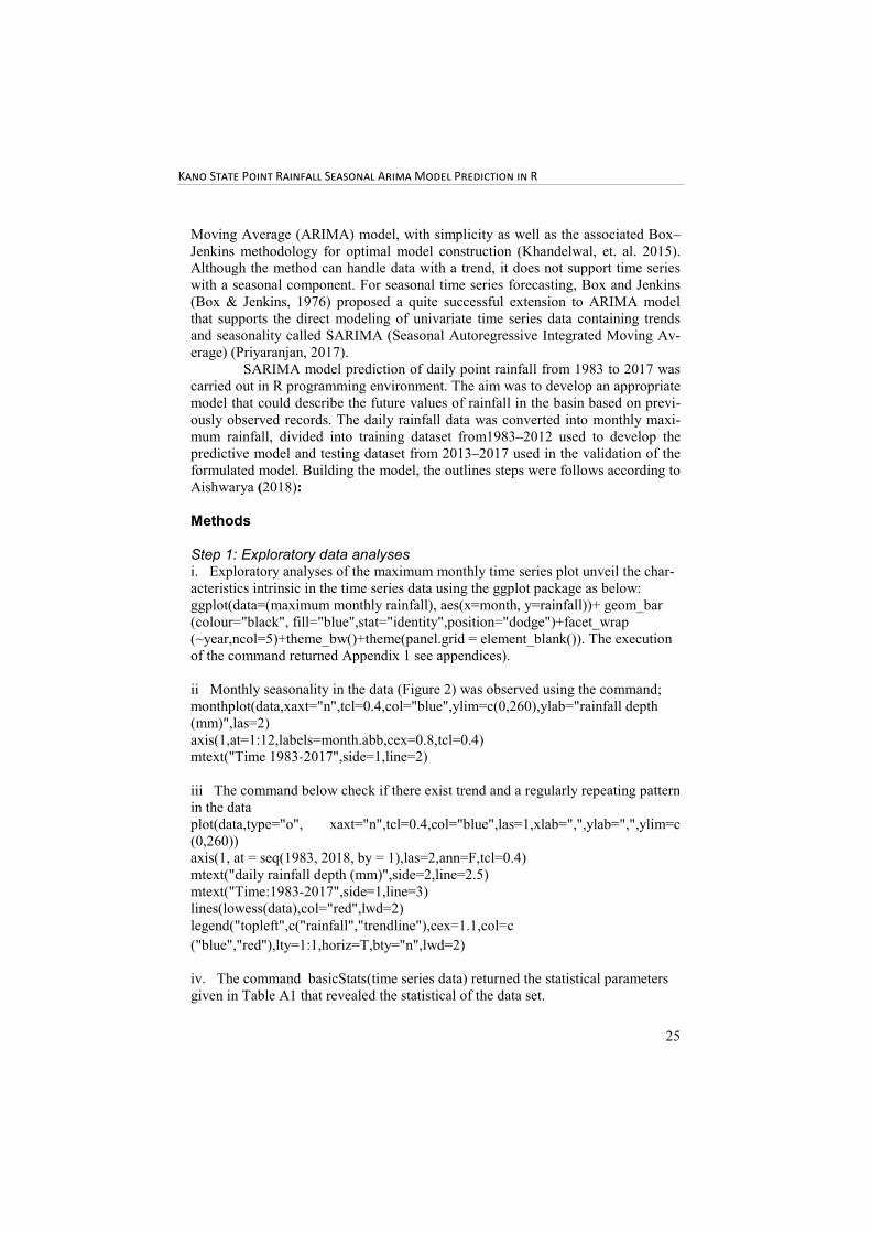
Methods Step 1: Exploratory data analyses

i. Exploratory analyses of the maximum monthly time series plot unveil the char-

acteristics intrinsic in the time series data using the ggplot package as below:

ggplot(data=(maximum monthly rainfall), aes(x=month, y=rainfall))+ geom_bar

(colour="black", fill="blue",stat="identity",position="dodge")+facet_wrap

(~year,ncol=5)+theme_bw()+theme(panel.grid = element_blank()). The execution

of the command returned Appendix 1 see appendices).

ii Monthly seasonality in the data (Figure 2) was observed using the command;

monthplot(data,xaxt="n",tcl=0.4,col="blue",ylim=c(0,260),ylab="rainfall depth

(mm)",las=2)

axis(1,at=1:12,labels=month.abb,cex=0.8,tcl=0.4)

mtext("Time 1983-2017",side=1,line=2)

iii The command below check if there exist trend and a regularly repeating pattern

in the data

plot(data,type="o", xaxt="n",tcl=0.4,col="blue",las=1,xlab=",",ylab=",",ylim=c

(0,260))

axis(1, at = seq(1983, 2018, by = 1),las=2,ann=F,tcl=0.4)

mtext("daily rainfall depth (mm)",side=2,line=2.5)

mtext("Time:1983-2017",side=1,line=3)

lines(lowess(data),col="red",lwd=2)

legend("topleft",c("rainfall","trendline"),cex=1.1,col=c

("blue","red"),lty=1:1,horiz=T,bty="n",lwd=2)

iv. The command basicStats(time series data) returned the statistical parameters

given in Table A1 that revealed the statistical of the data set.

S��

26

Step 2: Time series decomposition

The time series decomposition command fragmented the series into four compo-

nents; the observed data, the trend component, the seasonal component and the

random component. This was realized by the command below:

> plot(decompose(data))

Step 3: Auto Correlation factor (ACF) and Partial Auto Correlation factor (PACF) plot The Auto Correlation factor (ACF) and Partial Auto Correlation factor (PACF)

plot was obtained using the command below:

> acf2(data)

Step 4: Fitting the model and diagnostic test a. The first model parameter was determined by the command auto.arima() func-

tion within the forecast package.:

> model1 = auto.arima(data.train, stepwise = FALSE trace=T, test="kpss",

ic="aic")

The stepwise = FALSE, allows for a more in-depth search of potential models,

trace = TRUE, allows to get a list of all the investigated models fitting models us-

ing approximations to speed the model formulation.

b. the diagnostic test executed using the best selected model revealed the statisti-

cal significance of residual data, this include the residual plot, normal plot and the

p value for Ljung-Box statistic as shows in Figure 6. The command is as below;

> arma1=sarima(data.train, 6,0,2,0,1,3,12)

Step 5: validation or accuracy test done using the command accuracy > (arima1.forecast, data.test)

Step 6: Prediction for thirteen years (2018-2030) using the validated test model > fit<-arima(rf.ts,order =c(6,0,2),seasonal=list(order=c(0,1,3),period = 12))

> predict(fit, n.ahead = 12*13)

Results

K�� S� P�� R�� S�� A�� M�� P�� R

27

Exploratory Analysis:

Figure 1: Seasonal regularly repeating pattern with increasing trend

Figure 2: Monthly seasonality plot

S��

28

ACF and PACF plot:

Figure 3: ACF and PACF plots

Forecast model parameter estimation:

Table 1: Seasonal ARIMA model parameters

Model parameters (p,d,q)(P,D,Q)[m]

auto.arima (0,0,1)(0,1,2)[12]

sarima(data.train, 1,0,1,0,1,2,12)











AIC AICc BIC

3127.09 3127.27 3146.35

8.715259 8.715733 8.779641

8.714646 8.715311 8.789759

8.714781 8.715927 8.811354

8.744617 8.745511 8.830636

8.736105 8.736999 8.822124

8.712219 8.713656 8.819523

8.72059 8.722351 8.838624

8.716768 8.718887 8.845532

8.728608 8.730369 8.846642

8.756668 8.758439 8.874943

8.707182 8.709694 8.846677

K�� S� P�� R�� S�� A�� M�� P�� R

29

Fi�ed model diagnos�c test sta�s�cs:

Figure 4: Fitted model diagnostic test statistic

The predictive model output

Figure 5: Predictive model output

S��

30

Figure 6: Visual predictive model check

Predictive model accuracy check:

Table 2: Predictive model accuracy check

Discussions Figure 1 shows a seasonally repeating pattern with the presence of slowly increas-

ing trend observed in the time series indicating rises in rainfall over the years (1983

-2017). Figure 2 shows that appreciable rainfall begins in April and increases to the

August (the peak month), then decline to March. The short horizontal line repre-

sents the monthly rainfall mean.

Figure 3 shows the seasonal cycle of twelve (12) months period inherent

in the time series that revealed that the series can only be model by the application

of SARIMA. Table 1 gives the various model parameters obtained in the processes

of fitting the model. The best model parameter selected was sarima(6,0,2,0,1,3,12)

with minimum AIC: 8.707182, AICc: 8.709694 and BIC: 8.846677.

Figure 4: The ACF in the fitted model diagnostic test statistics shows a

white noise along with p values all above the significant level that confirmed the

performance level of the selected model parameter sarima (6,0,2,0,1,3,12). Figure

5 shows the predictive model output (2013-2017) follows the seasonal repeating

pattern that exist in the original data, this further validated the selected sarima

(6,0,2,0,1,3,12) parameter.

Figure 6 shows the visual predictive accuracy checks in both the test data

set (the black line) and the predicted data (the blue dash line) obtained. The plot

revealed that the model over predicted the time series. Table 2 shows that the mod-

el over fitted the original data with Mean Error (ME) of 8.65 and Error (MAE)

28.27.

Statistical inference Value obtained

Mean Error (ME) -8.65

Root Mean Square Error (RMSE) 28.27

Mean Absolute Error (MAE) 18.88

K�� S� P�� R�� S�� A�� M�� P�� R

31

Appendix 1 shows the characteristics of rainfall time series over period of

1983 to 2017 at glance. The y axis is the accumulated rainfall depth in mm and the

x axis is the months (1 to 12). Appendix 2 shows the time series decomposition

that consist of the raw data, the seasonal (stochastic) component, and the trend

(deterministic) component and error component in the time series.

Table A1 shows the statistic inherent in the time series. The series has a

positive skewness of value greater than 0 and a heavy tailed distribution of kurtosis

greater than 3.

Appendix 3 shows the predicted result per month for the year 2018 to

2030. All the negative values were due to over prediction of selected model, they

are considered as zeros since there is negative rainfall.

Conclusion In this paper, the SARIMA modelling procedure was applied to point rainfall data

to select the best modelling parameters and go further to make forecast. The time

series analysis revealed that is a seasonally repeated pattern of rainfall depth that

peaks in the month of August with its trough that begins from the month of No-

vember to March, with a weak increase in the accumulated rainfall amount across

1983 to 2017. The prediction results with a Mean Error (ME) of -8.65, Root Mean

Square Error (RMSE) of 28.27 and Mean Absolute Error (MAE) of 18.8 shows

that there will be a very weak decreases in rainfall amount from 2018 to 2030. The

time series is positively skewed with a Kurtosis greater than 3.

Correspondence

I.M. Sanni

Water Resources and Environmental and Engineering

Ahmadu Bello University

Zaria, Nigeria

Email: [email protected]

S��

32

References

Adhikari, R., and Agrawal, R. K. (2014). A combination of artificial neural net-

work and random walk models for financial time series forecasting. Neural

Computing and Applications 24 (6), 1441-1449.

Box, G. E. P., & Jenkins, G. M. (1976). Time series analysis forecasting and con-

trol Box, G.E.P. and Jenkins, G.M. (1976) Time Series Analysis, Fore-

casting and Control. Holden-Day, San Francisco.

Khandelwal, I., Adhikari, R., & Verma, G. (2015). Time Series Forecasting using

Hybrid ARIMA and ANN Models based on DWT Decomposition, 48

(2015) 173 – 179. Available online at www.sciencedirect.com doi:

10.1016/j.procs.2015.04.167.

Why Do We Need Rain? https://www.reference.com/science/need-rain-

33f74dd1e166e232 retrieved 12 August, 2019

Priyaranjan Pattnayak (2017): Monthly Auto Sales in US - Time Series Analysis

using SARIMA https://rstudio-

pubstat-

ic.s3.amazonaws.com/343096_90b218e393454f79a5012e7ad0913e76.htm

l

Aishwarya Singh, (2018): Build High Performance Time Series Models using Au-

to ARIMA in Python and R https://www.analyticsvidhya.com/

blog/2018/08/auto-arima-time-series-modeling-python-r/.

K�� S� P�� R�� S�� A�� M�� P�� R

33

Appendices Appendix 1

K�� E�� J�� .

34

Appendix 2

Table A1 : Basic statistics characteristics of the rainfall time series

nobs 420.00 1st Quartile 0.00 Sum 10920.40 Stdev

36.66

NAs 0.00 3rd Quartile 45.03 SE Mean 1.79 Skewness

2.11

Minimum 0.00 Mean 26.00 LCL Mean 22.48 Kurtosis

6.72

Maximum 241.00 Median 5.70 UCL Mean 29.52 Vari-

ance 1344.04

Appendix 3

K�� S� P�� R�� S�� A�� M�� P�� R

35

Kano State Point Rainfall Seasonal Arima Model Prediction in R

Documents

Transcript of Kano State Point Rainfall Seasonal Arima Model Prediction in R