Managing Energy and Carbon - CALU Centre for Alternative Land Use
Design of Control Systems
Steps to designing a controller:1 Determine the system’s design specifications2 Determine the uncompensated system’s performance3 Determine the controller’s configuration and its connection to the system4 Determine the controller’s parameters5 Test the compensated (controlled) system
Controller Configurations:
1- Series – Cascade compensation
2- Feedback Compensation
3- State Feedback Compensation (not covered here)
+ -
ControllerGc(s)
Controlled Process Gp(s)
+ -
+ -
ControllerGc(s)
Controlled Process Gp(s)
There are other types of related configurations.
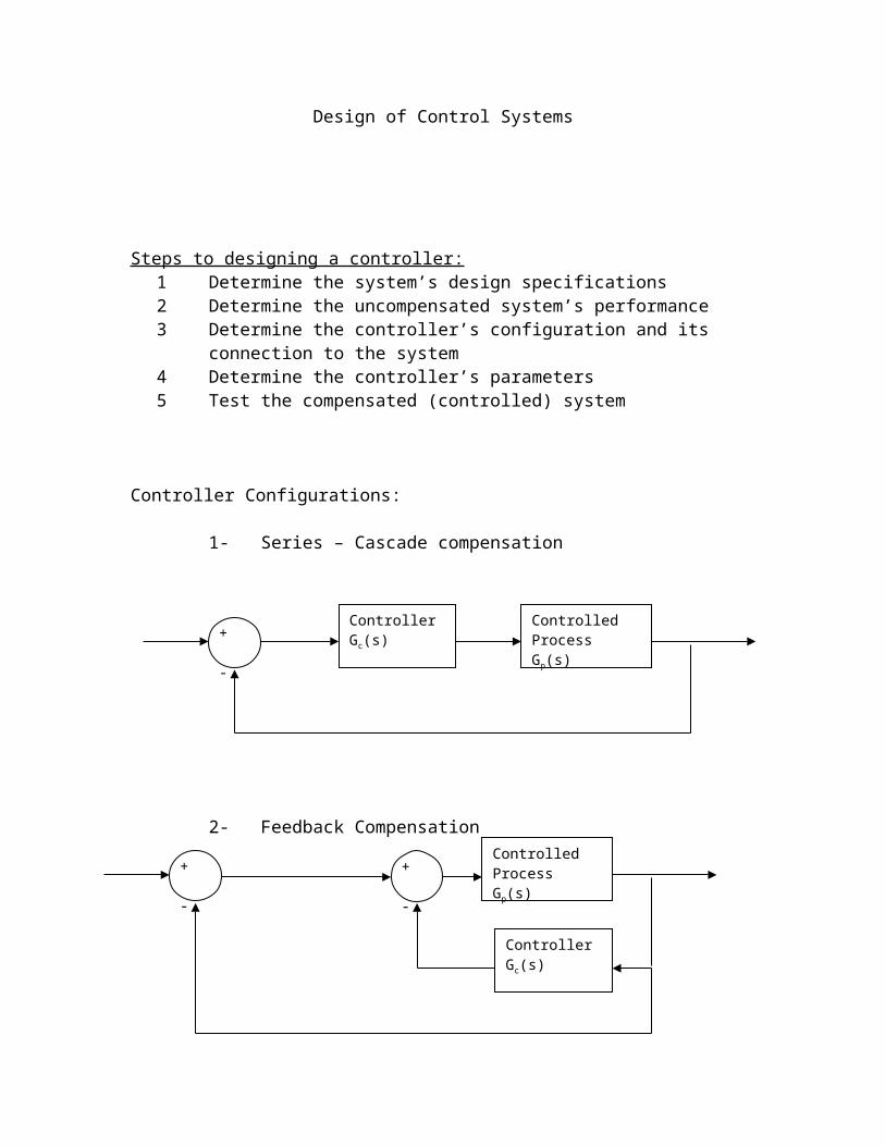
Summary of the time and frequency domain characteristics:
1- Complex poles of the closed loop transfer function lead to underdamped step response. If all the poles are real, the step response is overdamped. Zeros of the closed loop transfer function may cause overshoot even if the system is overdamped.
2- The response of the system is dominated by the poles closest to origin. Transients of those poles farther to the left decay faster.
3- The farther the poles to the left, the faster the decay and the greater the bandwidth is.
4- Time and frequency domain specifications are loosely associated with each other. Rise time and bandwidth are inversely proportional. Phase margin, gain margin, and damping ratio are inversely proportional.
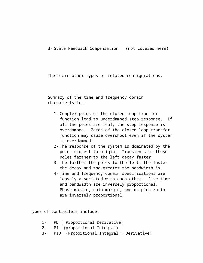
Types of controllers include:
1- PD ( Proportional Derivative)2- PI (proportional Integral)3- PID (Proportional Integral + Derivative)4- Phase Lead controller5- Phase Lag controller6- Lead-lag controller7- Pole zero cancellation8- pole placement9- State Feedback10- State Feedback with integral control11- Robust control12- Optimal control13- Adaptive control
Note: The controls we have done with adjustable gain, K are referred to as Proportional Control.
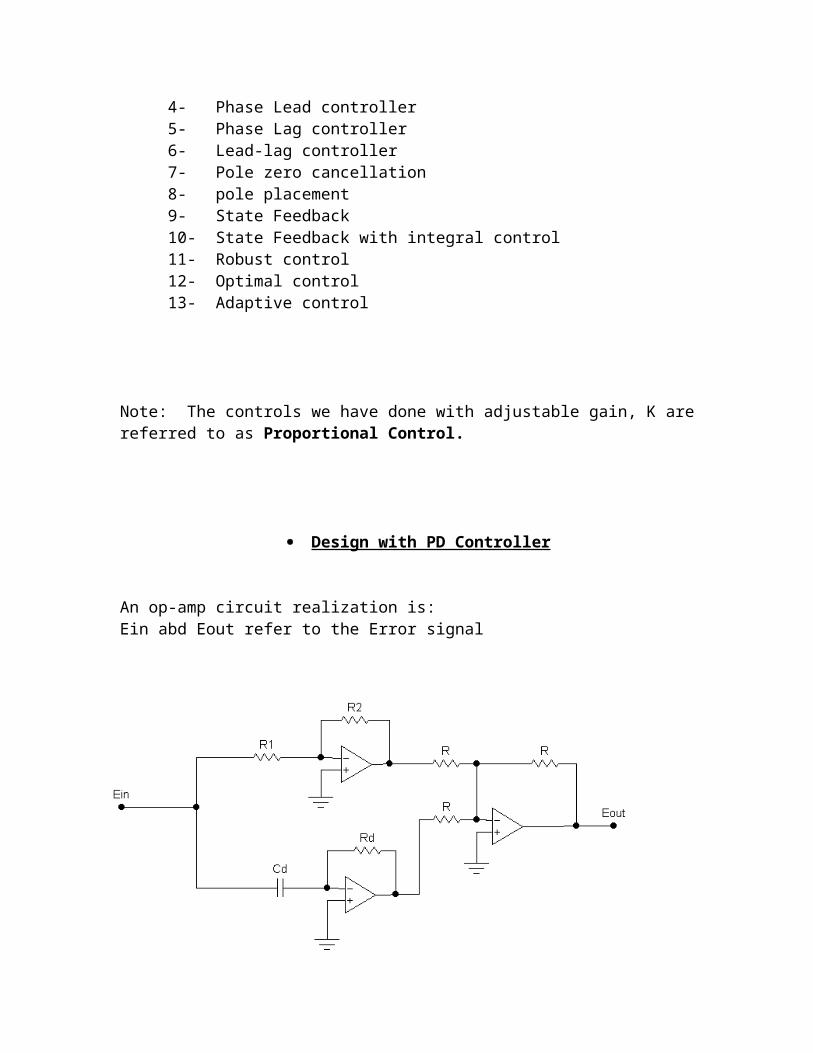
Design with PD Controller
An op-amp circuit realization is:Ein abd Eout refer to the Error signal
The related equations are:
eout(t) = K p ein ( t )+Kd
de in( t )dt
In the s-domain:
Eout (s )Ein( s )
=Gc( s )=R2
R1+RdCd s
Where: Kp=R2/R1 and Kd = RdCd
Therefore:The controller’s transfer function is:
Gc(s) = Kp + Kd S = K p (1+
KdK ps)
(this is the standard form)
Notes on PD Controller/Compensator:
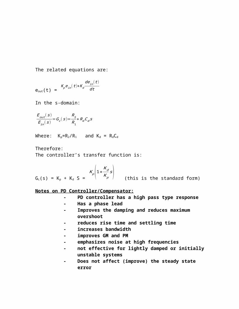
- PD controller has a high pass type response- Has a phase lead- Improves the damping and reduces maximum overshoot- reduces rise time and settling time- increases bandwidth- improves GM and PM- emphasizes noise at high frequencies- not effective for lightly damped or initially unstable systems- Does not affect (improve) the steady state error
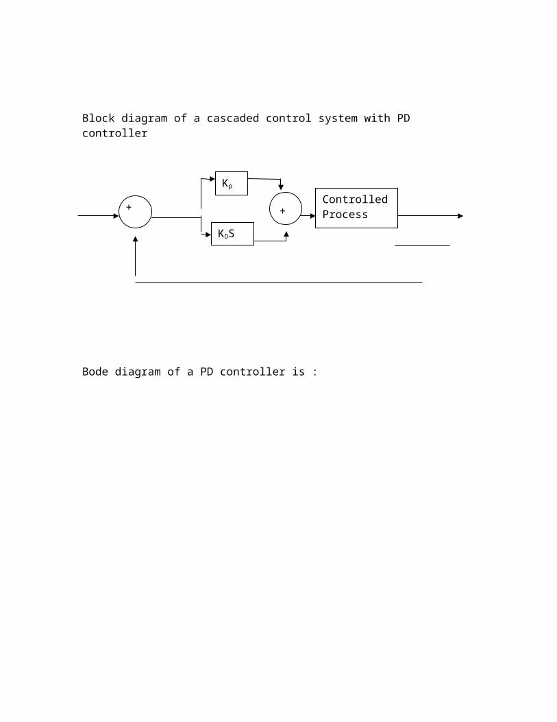
Block diagram of a cascaded control system with PD controller
Bode diagram of a PD controller is :
Controlled Process Gp(s)
Kp
+ -
KDS
+ +
From the figure:1- phase lead property is clearly apparent – it is used to improve the
phase margin of the system2- The magnitude characteristics push the gain-cross over frequency to
higher values.3- Based on 1 and 2, the design principle of the PD controller involves
the placing of the corner frequency of the controller at ω= Kp/Kd such that an effective improvement of the phase margin is realized at the new gain –cross over frequency.
4- For a given system, there is a range of value of Kp/Kd that is optimal for improving the damping of the system (notice the sentence – “damping of system”.)
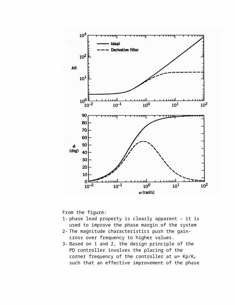
5- Select the values of Kp and Kd while considering physical implementation of the PD controller.
Example:
Given the second order model of an aircraft altitude control with the feedforward transfer function:
Gp (s )=4500 ks( s+361 . 2)
and the performance specifications are:1- steady state error due to a unit ramp input ¿ 0.0004432- maximum overshoot ¿ 5%3- rise time ¿ 0.005 seconds4- settling time ¿ 0.005 seconds
Solution:
To satisfy the maximum steady state error requirement:
Ess = ?
C = GE
C= G1+G
R
Therefore,
E= R1+G
E= R
1+ 4500Ks (s+361.2)
=R s(s+361.2)s ( s+361.2 )+4500 K
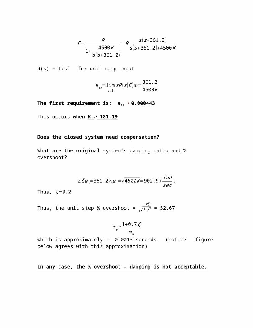
R(s) = 1/s2 for unit ramp input
ess=lims→0
sR (s )E ( s )= 361.24500K
The first requirement is: ess ¿ 0.000443
This occurs when K ≥ 181.19
Does the closed system need compensation?
What are the original system’s damping ratio and % overshoot?
2 ζ ωn=361.2∧ωn=√4500K=902.97 radsec
.
Thus, ζ=0.2
Thus, the unit step % overshoot = e−πζ
√1−ζ 2 = 52.67
t r≅1+0.7 ζωn
which is approximately = 0.0013 seconds. (notice – figure below agrees with this approximation)
In any case, the % overshoot – damping is not acceptable.
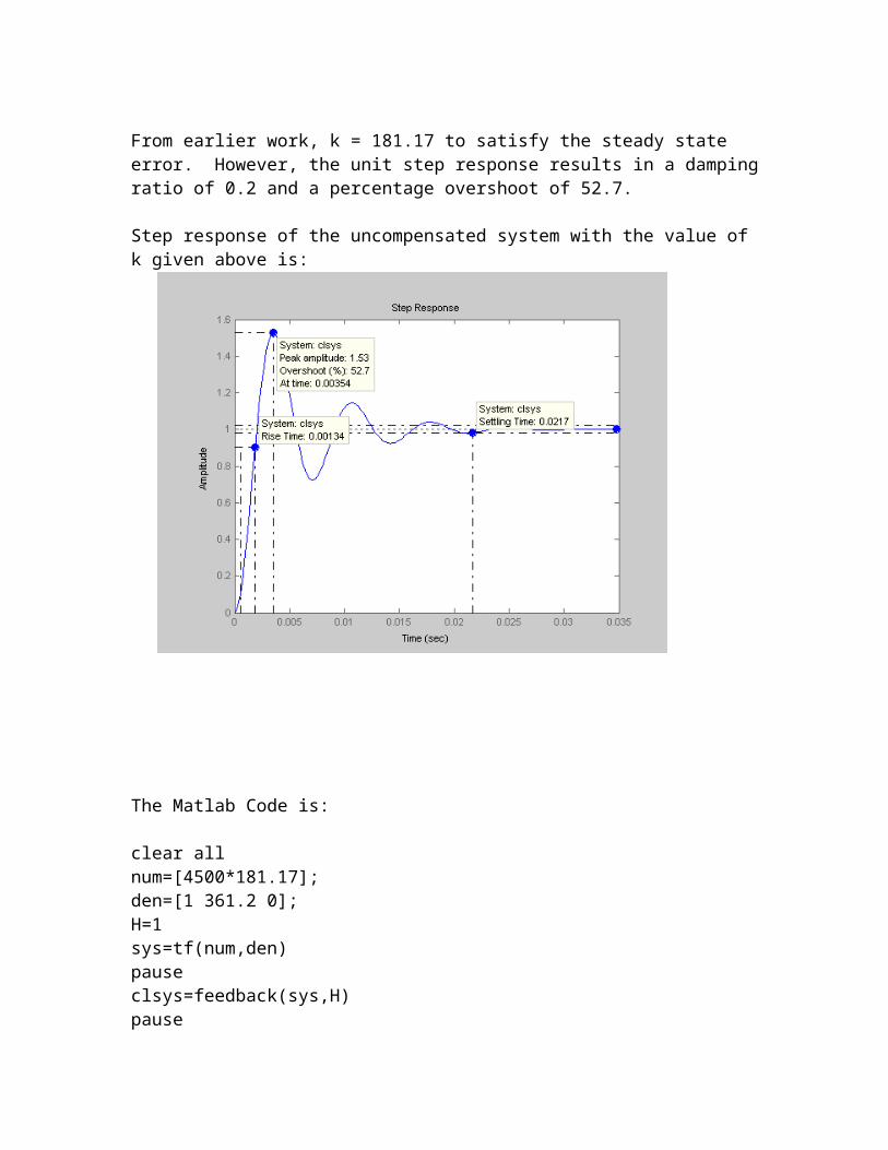
From earlier work, k = 181.17 to satisfy the steady state error. However, the unit step response results in a damping ratio of 0.2 and a percentage overshoot of 52.7.
Step response of the uncompensated system with the value of k given above is:
The Matlab Code is:
clear allnum=[4500*181.17];den=[1 361.2 0];H=1sys=tf(num,den)pauseclsys=feedback(sys,H)pausestep(clsys)
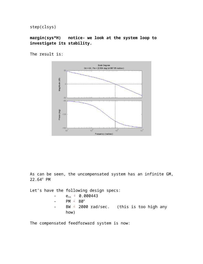
margin(sys*H) notice- we look at the system loop to investigate its stability.
The result is:
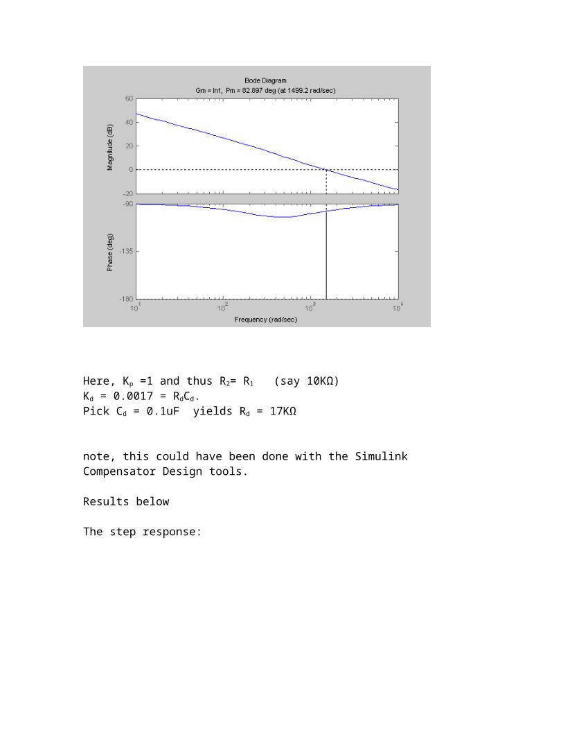
As can be seen, the uncompensated system has an infinite GM, 22.64o PM
Let’s have the following design specs:- ess ¿ 0.000443- PM ¿ 80o
- BW ¿ 2000 rad/sec. (this is too high any how)
The compensated feedforward system is now:
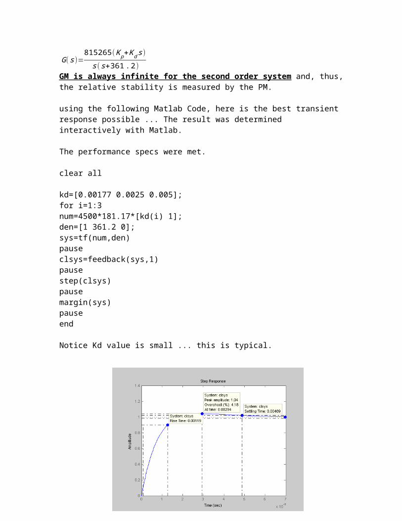
G( s )=815265(K p+Kd s )s (s+361. 2 )
GM is always infinite for the second order system and, thus, the relative stability is measured by the PM.
using the following Matlab Code, here is the best transient response possible ... The result was determined interactively with Matlab.
The performance specs were met.
clear all
kd=[0.00177 0.0025 0.005];for i=1:3num=4500*181.17*[kd(i) 1];den=[1 361.2 0];sys=tf(num,den)pauseclsys=feedback(sys,1)pausestep(clsys)pausemargin(sys)pauseend
Notice Kd value is small ... this is typical.
Here, Kp =1 and thus R2= R1 (say 10KΩ)Kd = 0.0017 = RdCd.Pick Cd = 0.1uF yields Rd = 17KΩ
note, this could have been done with the Simulink Compensator Design tools.
Results below
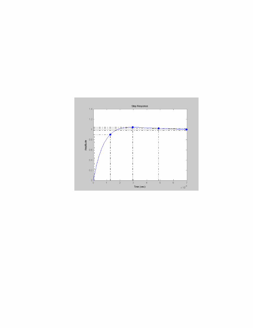
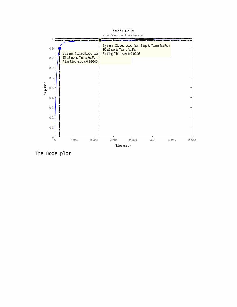
The step response:Step Response
Time (sec)
Ampl
itude
0 0.002 0.004 0.006 0.008 0.01 0.012 0.0140
0.1
0.2
0.3
0.4
0.5
0.6
0.7
0.8
0.9
1
System: Closed Loop from Step to Transfer FcnI/O: Step to Transfer FcnRise Time (sec): 0.00049
System: Closed Loop from Step to Transfer FcnI/O: Step to Transfer FcnSettling Time (sec): 0.0046
From: Step To: Transfer Fcn
The Bode plot
101
102
103
104
-180
-135
-90
-45
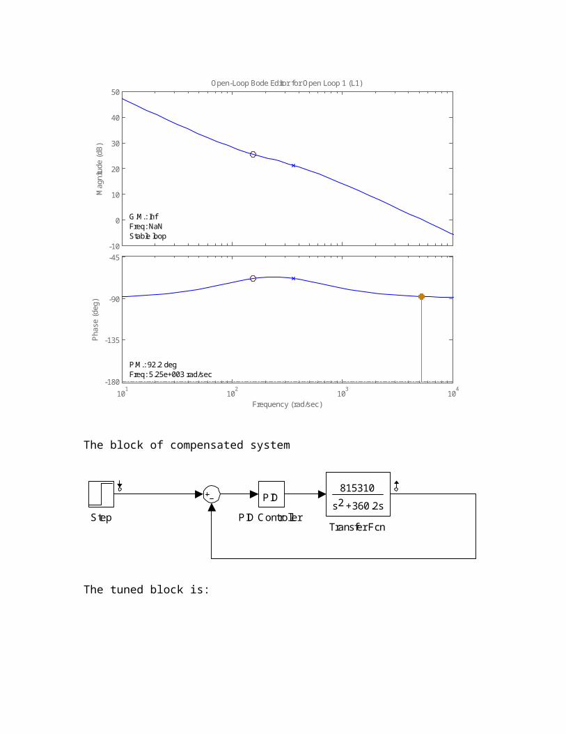
P.M.: 92.2 degFreq: 5.25e+003 rad/sec
Frequency (rad/sec)
Phas
e (d
eg)
-10
0
10
20
30
40
50
G.M.: InfFreq: NaNStable loop
Open-Loop Bode Editor for Open Loop 1 (L1)
Mag
nitu
de (d
B)
The block of compensated system
Transfer Fcn
815310
s +360.2s2Step PID Controller
PID
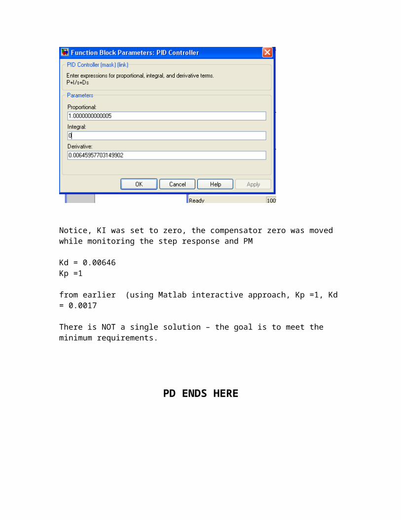
The tuned block is:
Notice, KI was set to zero, the compensator zero was moved while monitoring the step response and PM
Kd = 0.00646Kp =1
from earlier (using Matlab interactive approach, Kp =1, Kd = 0.0017
There is NOT a single solution – the goal is to meet the minimum requirements.
PD ENDS HERE
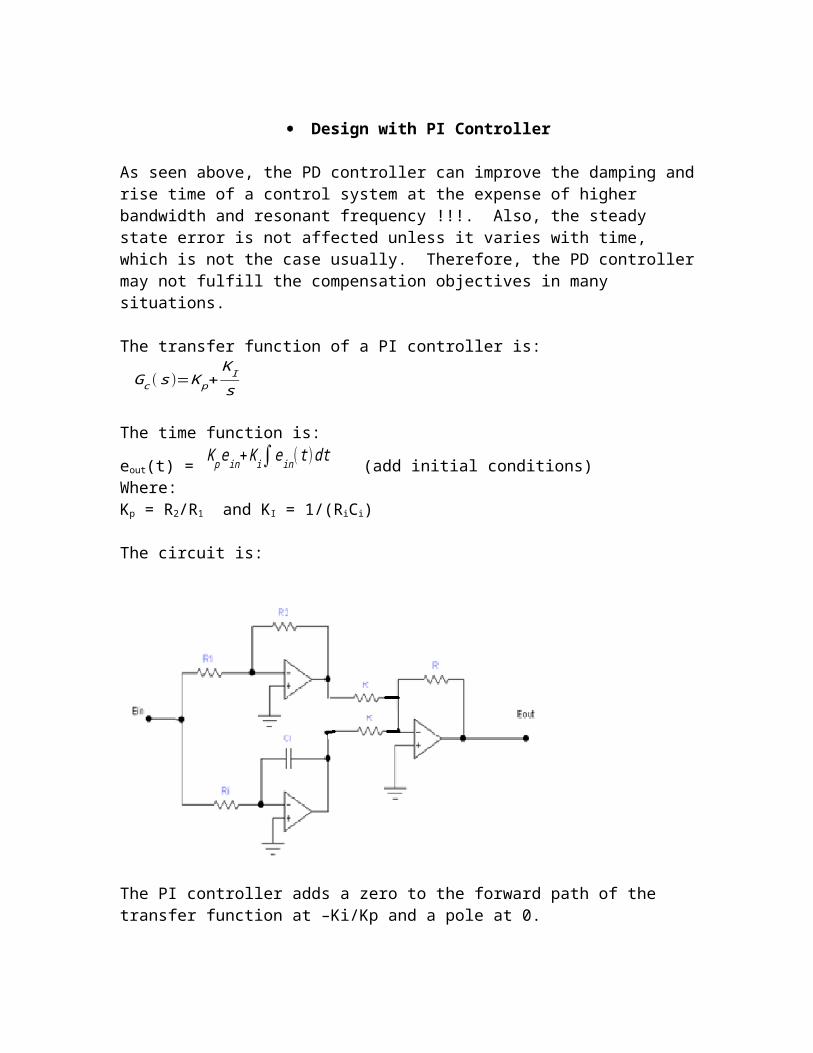
Design with PI Controller
As seen above, the PD controller can improve the damping and rise time of a control system at the expense of higher bandwidth and resonant frequency !!!. Also, the steady state error is not affected unless it varies with time, which is not the case usually. Therefore, the PD controller may not fulfill the compensation objectives in many situations.
The transfer function of a PI controller is:
Gc( s )=K p+K Is
The time function is:
eout(t) = K p ein+K i∫ ein ( t )dt (add initial conditions)Where:Kp = R2/R1 and KI = 1/(RiCi)
The circuit is:
The PI controller adds a zero to the forward path of the transfer function at –Ki/Kp and a pole at 0.
Kp
sK i
+ +
+ - )2(
2
n
n
wssKw
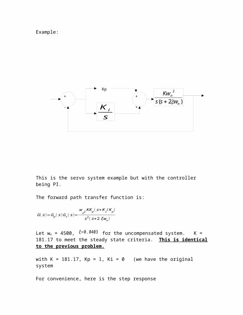
Example:
This is the servo system example but with the controller being PI.
The forward path transfer function is:
G( s )=Gp (s )Gc( s)=wn2KK p( s+K i /K p )
s2 (s+2ξwn )
Let wn = 4500, ξ=0.0403 for the uncompensated system. K = 181.17 to meet the steady state criteria. This is identical to the previous problem.
with K = 181.17, Kp = 1, Ki = 0 (we have the original system
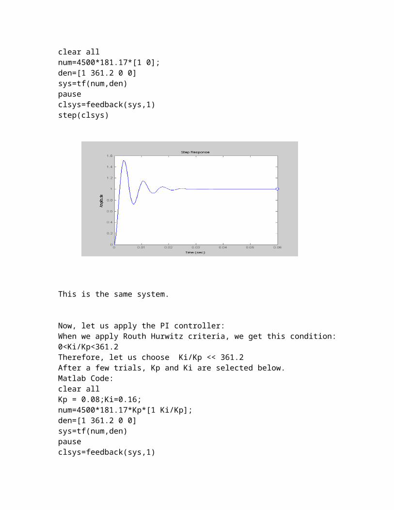
For convenience, here is the step responseclear allnum=4500*181.17*[1 0];den=[1 361.2 0 0]sys=tf(num,den)pauseclsys=feedback(sys,1)step(clsys)
This is the same system.
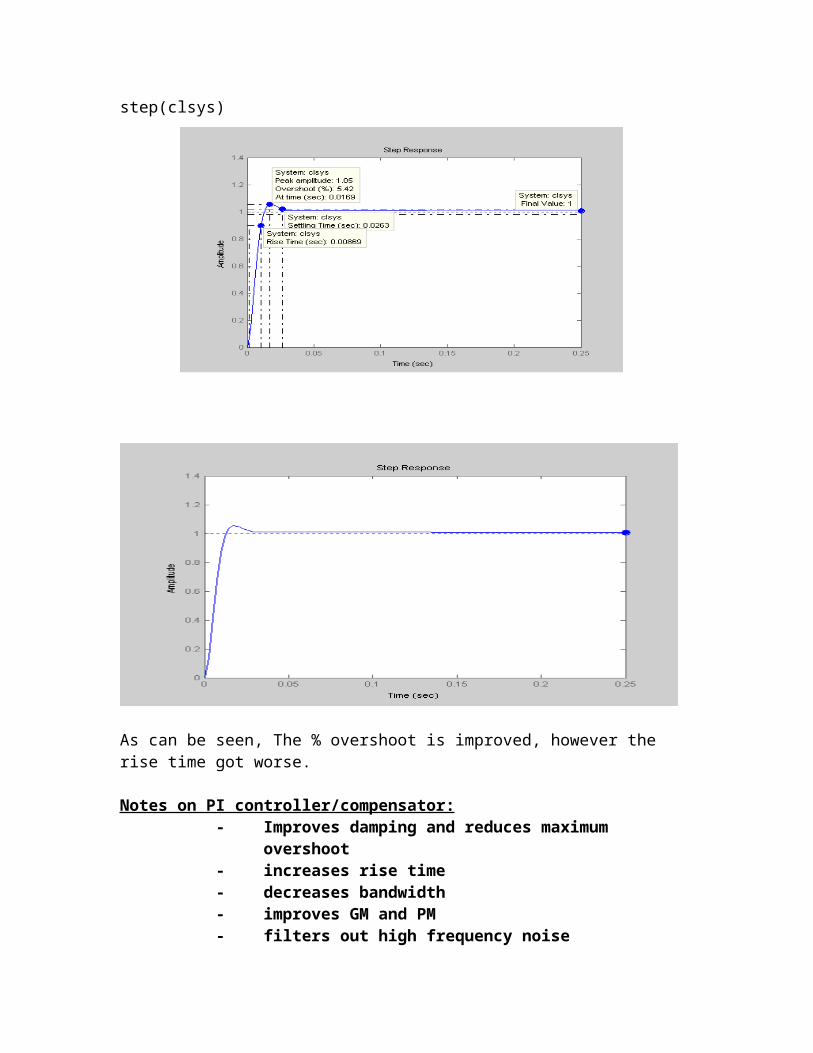
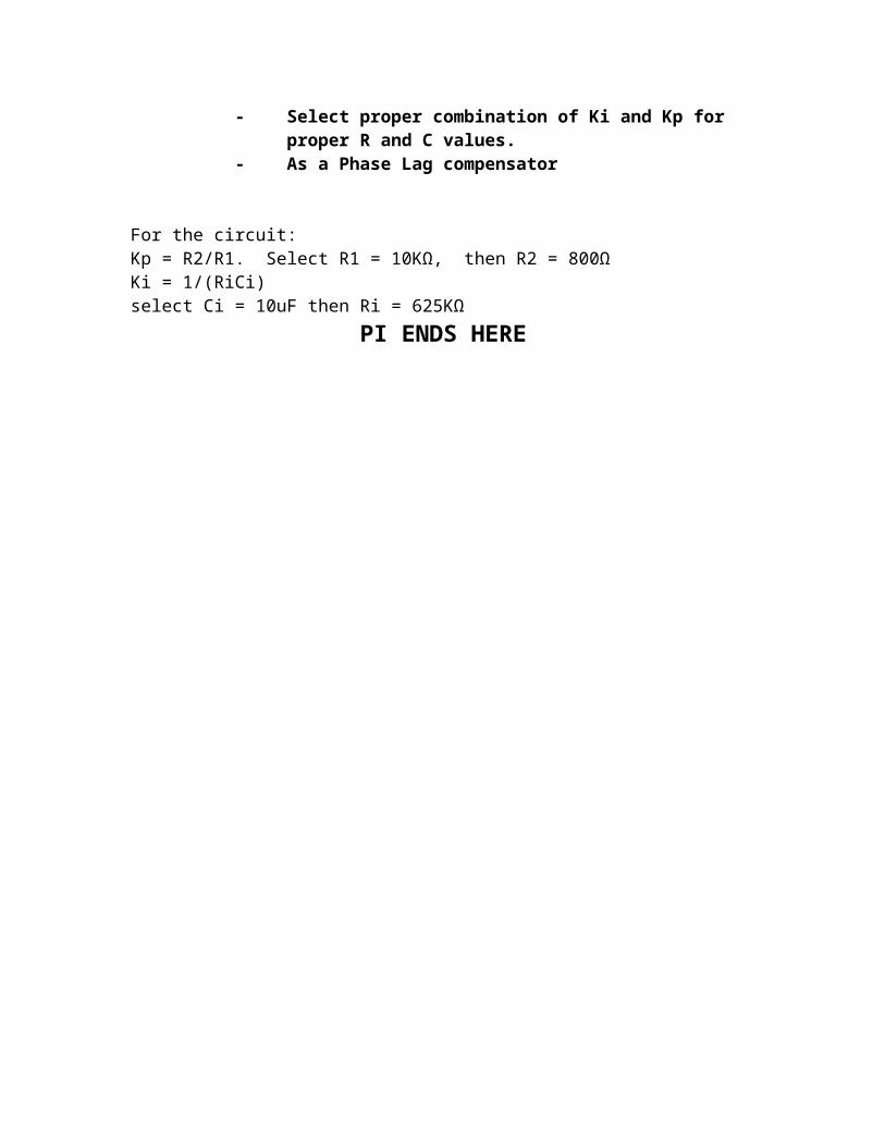
Now, let us apply the PI controller:When we apply Routh Hurwitz criteria, we get this condition:0<Ki/Kp<361.2Therefore, let us choose Ki/Kp << 361.2After a few trials, Kp and Ki are selected below.Matlab Code:clear allKp = 0.08;Ki=0.16;num=4500*181.17*Kp*[1 Ki/Kp];den=[1 361.2 0 0]sys=tf(num,den)pauseclsys=feedback(sys,1)step(clsys)
As can be seen, The % overshoot is improved, however the rise time got worse.
Notes on PI controller/compensator:- Improves damping and reduces maximum overshoot- increases rise time- decreases bandwidth- improves GM and PM- filters out high frequency noise- Select proper combination of Ki and Kp for proper R and C
values.- As a Phase Lag compensator
For the circuit:Kp = R2/R1. Select R1 = 10KΩ, then R2 = 800ΩKi = 1/(RiCi)select Ci = 10uF then Ri = 625KΩ
PI ENDS HERE

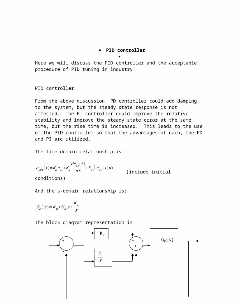
PID controller
Here we will discuss the PID controller and the acceptable procedure of PID tuning in industry.
PID controller
From the above discussion, PD controller could add damping to the system, but the steady state response is not affected. The PI controller could improve the relative stability and improve the steady state error at the same time, but the rise time is increased. This leads to the use of the PID controller so that the advantages of each, the PD and PI are utilized.
The time domain relationship is:
eout (t )=K p ein+K dde in( t )dt
+K i∫ ein (τ )dτ (include initial conditions)
And the s-domain relationship is:
Gc( s )=K p+Kd s+K is
The block diagram representation is:
Kp
K is
+ + +
+ -
Gp(s)
Kd s
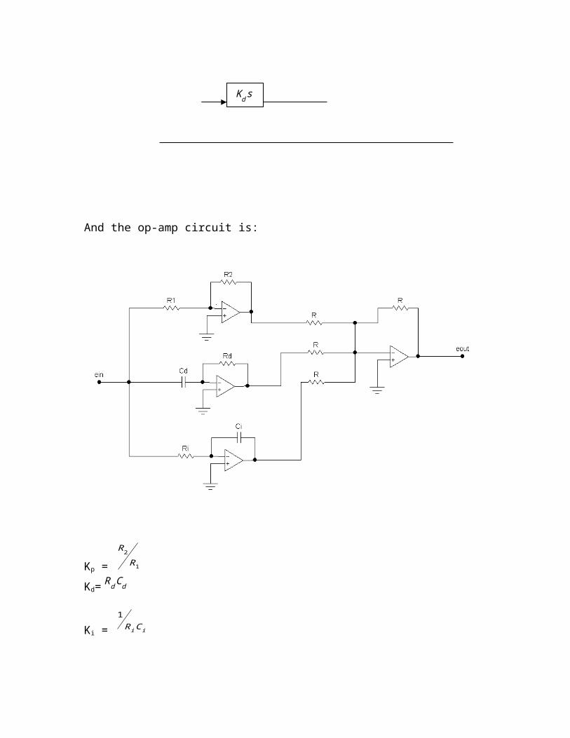
And the op-amp circuit is:
Kp =
R2
R1
Kd=RdCd
Ki = 1RiCi
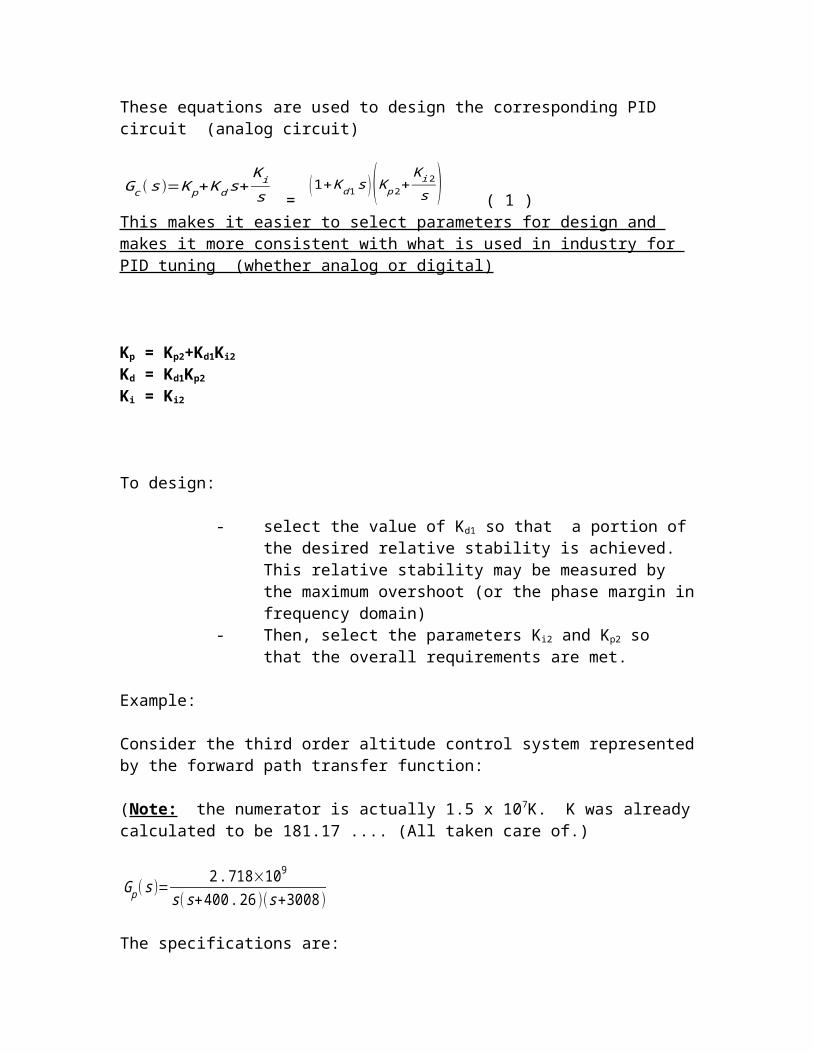
These equations are used to design the corresponding PID circuit (analog circuit)
Gc( s )=K p+Kd s+K is =
(1+K d 1s )(K p 2+K i 2s )
( 1 ) This makes it easier to select parameters for design and makes it more consistent with what is used in industry for PID tuning (whether analog or digital)
Kp = Kp2+Kd1Ki2
Kd = Kd1Kp2
Ki = Ki2
To design:
- select the value of Kd1 so that a portion of the desired relative stability is achieved. This relative stability may be measured by the maximum overshoot (or the phase margin in frequency domain)
- Then, select the parameters Ki2 and Kp2 so that the overall requirements are met.
Example:
Consider the third order altitude control system represented by the forward path transfer function:
(Note: the numerator is actually 1.5 x 10⁷K. K was already calculated to be 181.17 .... (All taken care of.)
Gp (s )=2 .718×109
s( s+400 .26 )(s+3008 )
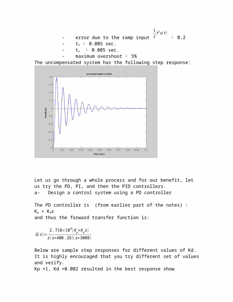
The specifications are:
- error due to the ramp input
12t 2u ( t )
¿ 0.2- tr ¿ 0.005 sec.- ts ¿ 0.005 sec.- maximum overshoot ¿ 5%
The uncompensated system has the following step response:
Let us go through a whole process and for our benefit, let us try the PD, PI, and then the PID controllers.a- Design a control system using a PD controller
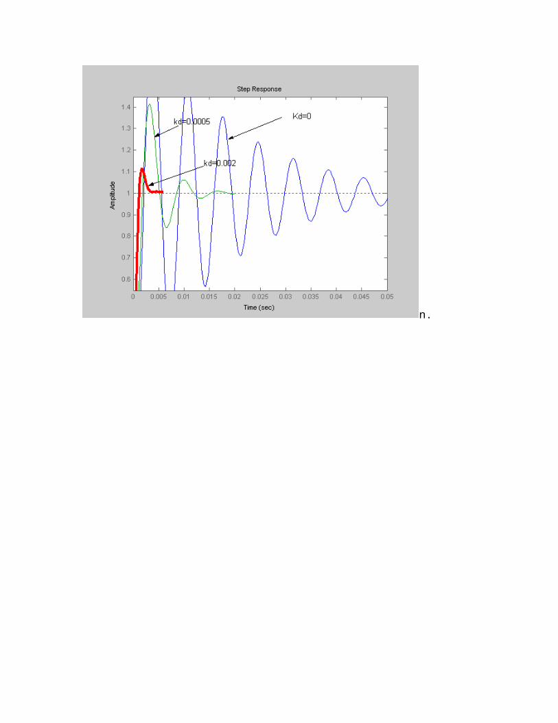
The PD controller is (from earlier part of the notes) :Kp + Kdsand thus the forward transfer function is:
G( s )=2.718×10⁹(K p+Kd s )s (s+400 .26 )( s+3008 )
Below are sample step responses for different values of Kd. It is highly encouraged that you try different set of values and verify.Kp =1, Kd =0.002 resulted in the best response show
n.
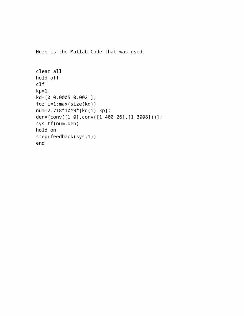
Here is the Matlab Code that was used:
clear allhold offclfkp=1;kd=[0 0.0005 0.002 ];for i=1:max(size(kd))num=2.718*10^9*[kd(i) kp];den=[conv([1 0],conv([1 400.26],[1 3008]))];sys=tf(num,den)hold onstep(feedback(sys,1))end
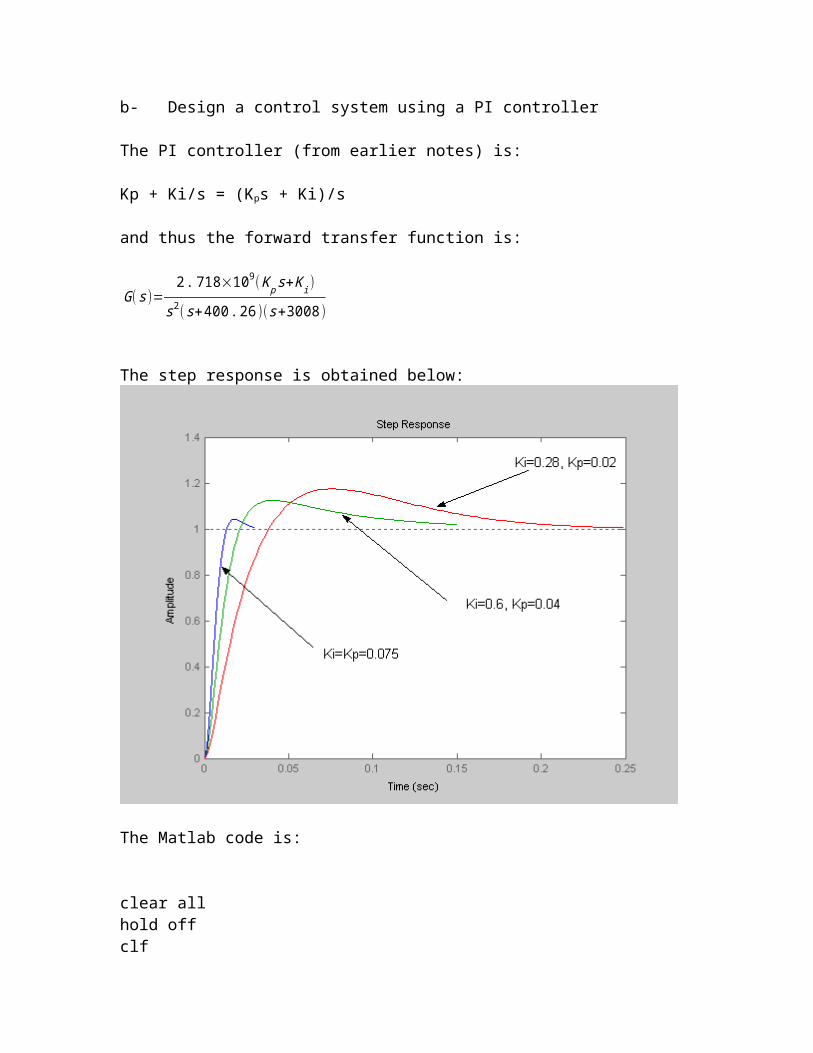
b- Design a control system using a PI controller
The PI controller (from earlier notes) is:
Kp + Ki/s = (Kps + Ki)/s
and thus the forward transfer function is:
G( s )=2 .718×109 (K ps+K i )
s2( s+400 . 26 )(s+3008)
The step response is obtained below:
The Matlab code is:
clear allhold offclfkp=[0.075 0.04 0.02];ki=[0.075 0.6 0.28];for i=1:max(size(ki))
num=2.718*10^9*[kp(i) ki(i)];den=[conv([1 0 0],conv([1 400.26],[1 3008]))];sys=tf(num,den)hold onstep(feedback(sys,1))end
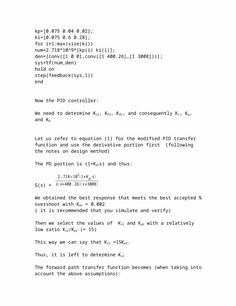
Now the PID controller:
We need to determine Ki2, KP2, Kd1, and consequently Ki, Kp, and Kd
Let us refer to equation (1) for the modified PID transfer function and use the derivative portion first (following the notes on design method)
The PD portion is (1+Kd1s) and thus:
G(s) =
2. 718×109(1+Kd 1 s )s (s+400 . 26)( s+3008 )
We obtained the best response that meets the best accepted % overshoot with Kd1 = 0.002( it is recommended that you simulate and verify)
Then we select the values of Ki2 and Kp2 with a relatively low ratio Ki2/Kp2 (= 15)
This way we can say that Ki2 =15Kp2.
Thus, it is left to determine Ki2
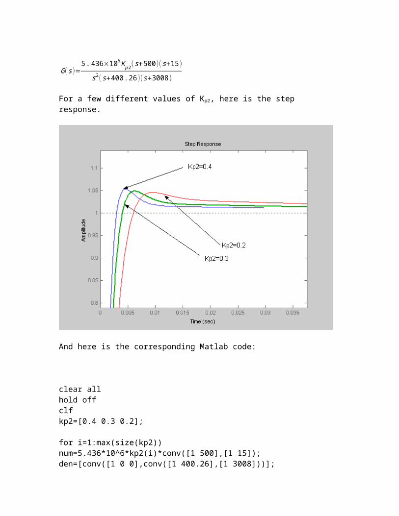
The forward path transfer function becomes (when taking into account the above assumptions):
G( s )=5 .436×106K p2 (s+500)( s+15 )
s2( s+400 .26 )(s+3008 )
For a few different values of Kp2, here is the step response.
And here is the corresponding Matlab code:
clear allhold offclfkp2=[0.4 0.3 0.2];
for i=1:max(size(kp2))num=5.436*10^6*kp2(i)*conv([1 500],[1 15]);den=[conv([1 0 0],conv([1 400.26],[1 3008]))];sys=tf(num,den)hold onstep(feedback(sys,1))end
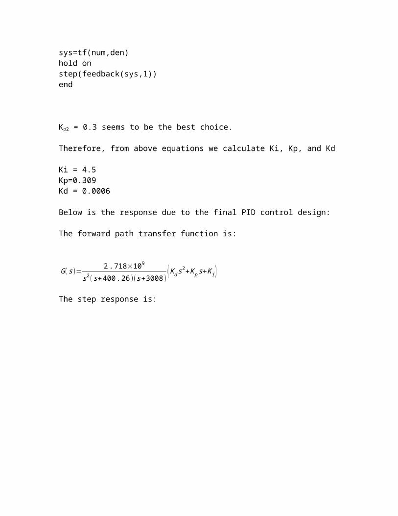
Kp2 = 0.3 seems to be the best choice.
Therefore, from above equations we calculate Ki, Kp, and Kd
Ki = 4.5Kp=0.309Kd = 0.0006
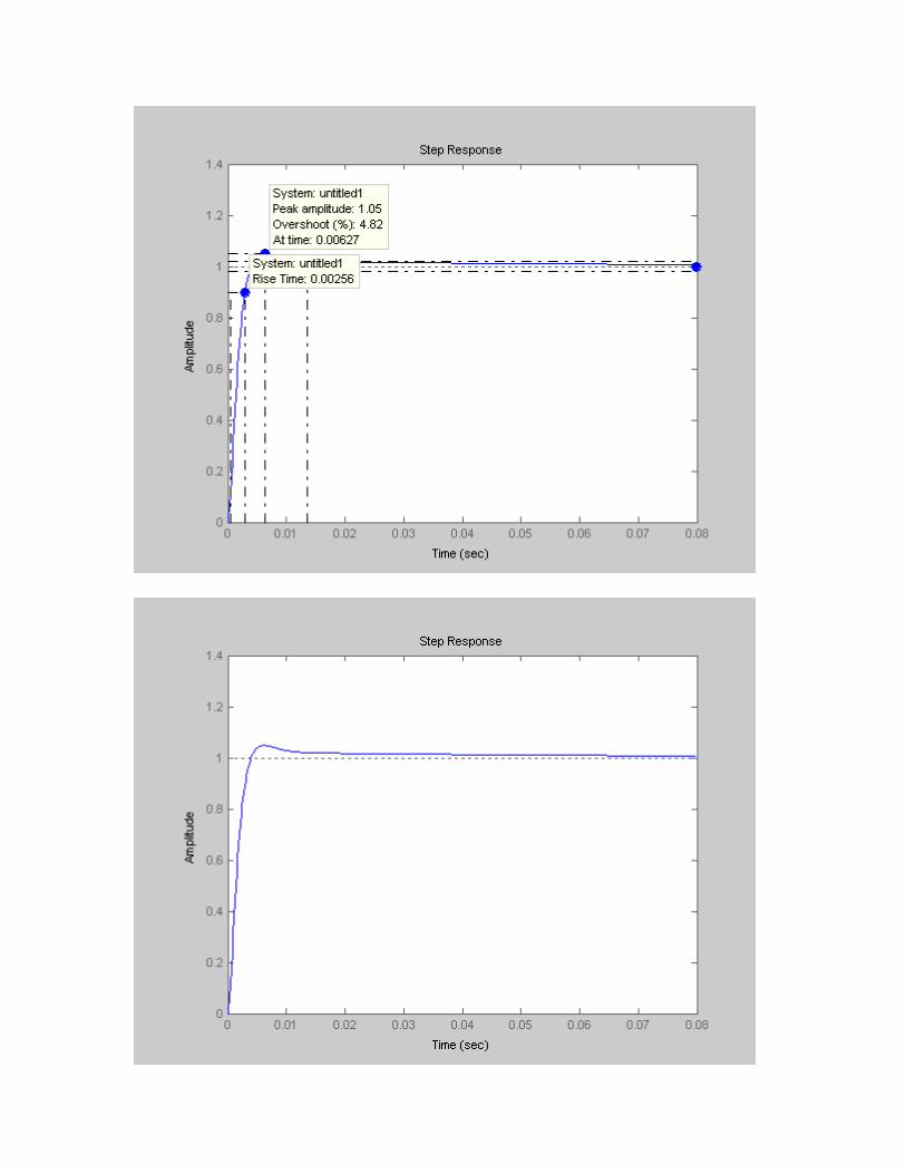
Below is the response due to the final PID control design:
The forward path transfer function is:
G( s )= 2 .718×109
s2( s+400 . 26 )(s+3008)(Kd s2+K ps+K i)
The step response is:
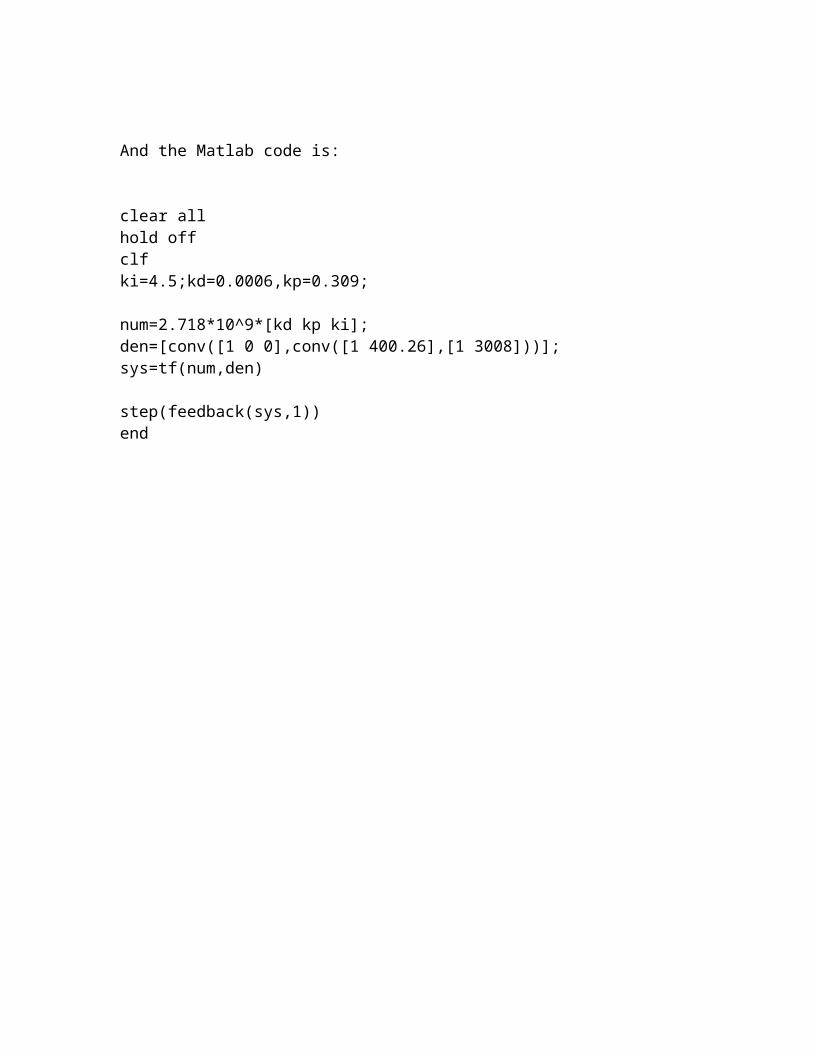
And the Matlab code is:
clear allhold offclfki=4.5;kd=0.0006,kp=0.309;
num=2.718*10^9*[kd kp ki];den=[conv([1 0 0],conv([1 400.26],[1 3008]))];sys=tf(num,den)
step(feedback(sys,1))end
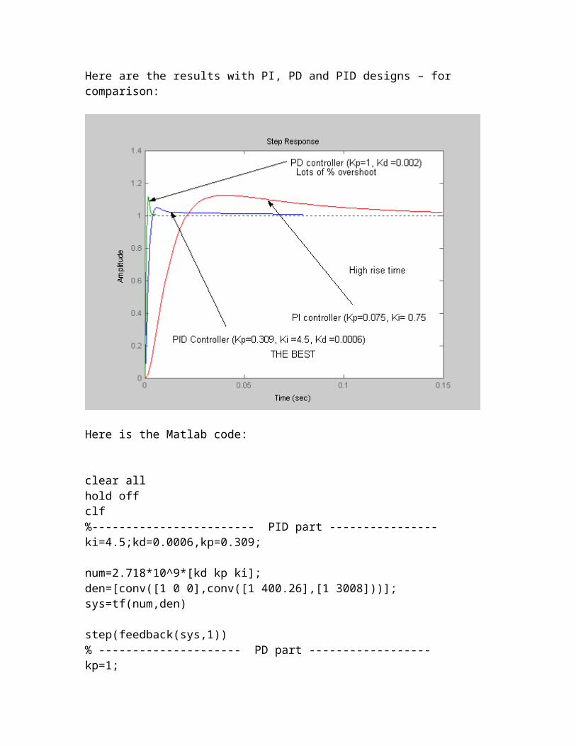
Here are the results with PI, PD and PID designs – for comparison:
Here is the Matlab code:
clear allhold offclf%------------------------ PID part ----------------ki=4.5;kd=0.0006,kp=0.309;
num=2.718*10^9*[kd kp ki];den=[conv([1 0 0],conv([1 400.26],[1 3008]))];sys=tf(num,den)
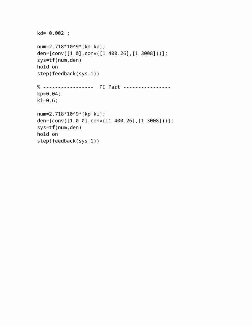
step(feedback(sys,1))% --------------------- PD part ------------------kp=1;kd= 0.002 ;
num=2.718*10^9*[kd kp];den=[conv([1 0],conv([1 400.26],[1 3008]))];sys=tf(num,den)
hold onstep(feedback(sys,1))
% ----------------- PI Part ----------------kp=0.04;ki=0.6;
num=2.718*10^9*[kp ki];den=[conv([1 0 0],conv([1 400.26],[1 3008]))];sys=tf(num,den)hold onstep(feedback(sys,1))
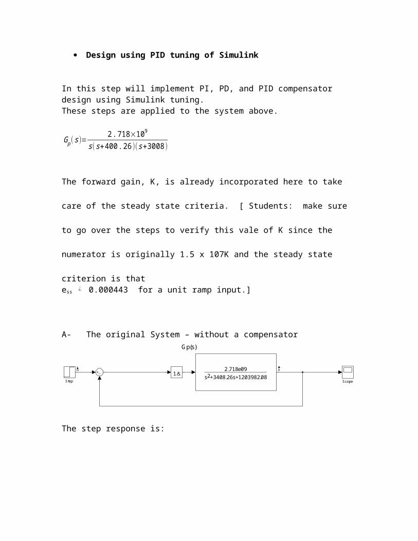
Design using PID tuning of Simulink
In this step will implement PI, PD, and PID compensator design using Simulink tuning.These steps are applied to the system above.
Gp (s )=2 .718×109
s( s+400 .26 )(s+3008 )
The forward gain, K, is already incorporated here to take care of the steady state criteria.
[ Students: make sure to go over the steps to verify this vale of K since the numerator is
originally 1.5 x 10⁷K and the steady state criterion is that ess ¿ 0.000443 for a unit ramp input.]
A- The original System – without a compensatorGp(s)
2.718e09s +3408.26s+1203982.082
Step Scope
1/s
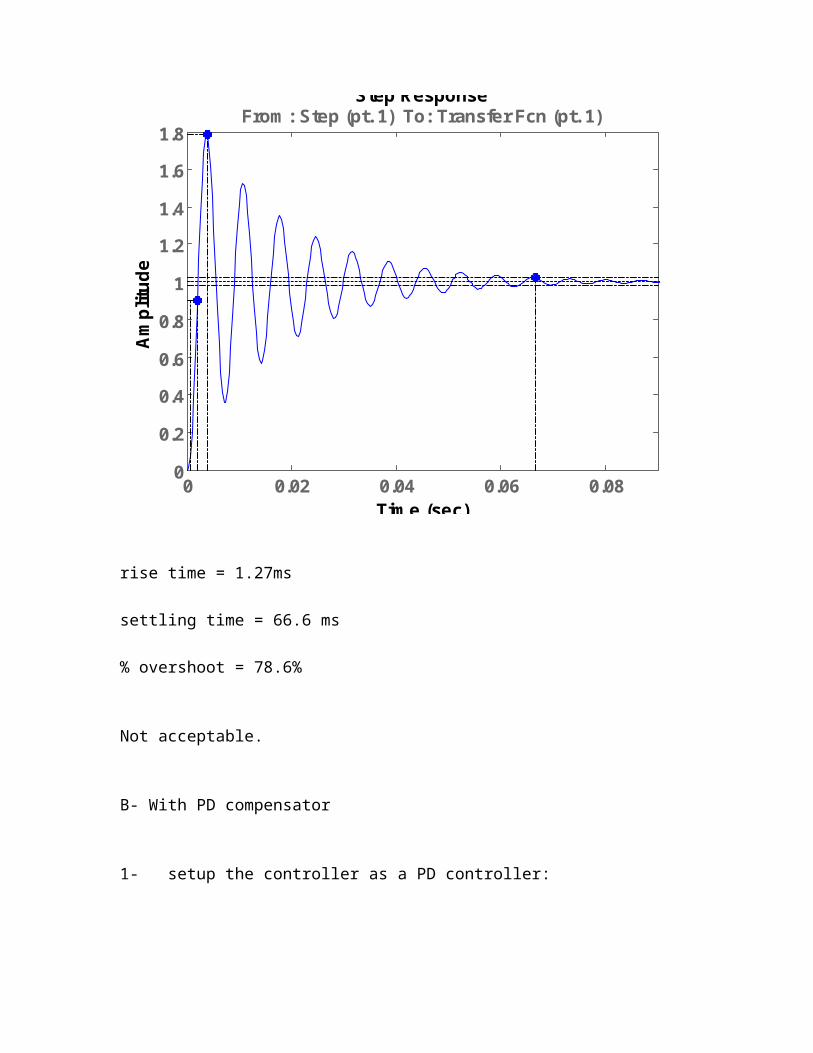
The step response is:
Step Response
Time (sec)
Am
plitu
de
0 0.02 0.04 0.06 0.080
0.2
0.4
0.6
0.8
1
1.2
1.4
1.6
1.8From: Step (pt. 1) To: Transfer Fcn (pt. 1)
rise time = 1.27ms
settling time = 66.6 ms
% overshoot = 78.6%
Not acceptable.
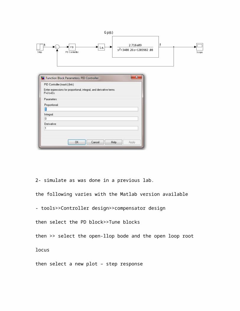
B- With PD compensator
1- setup the controller as a PD controller:
Gp(s)
2.718e09
s +3408 .26s+1203982 .082Step ScopePD Controller
PID 1/s
2- simulate as was done in a previous lab.
the following varies with the Matlab version available
- tools>>Controller design>>compensator design
then select the PD block>>Tune blocks
then >> select the open-llop bode and the open loop root locus
then select a new plot – step response
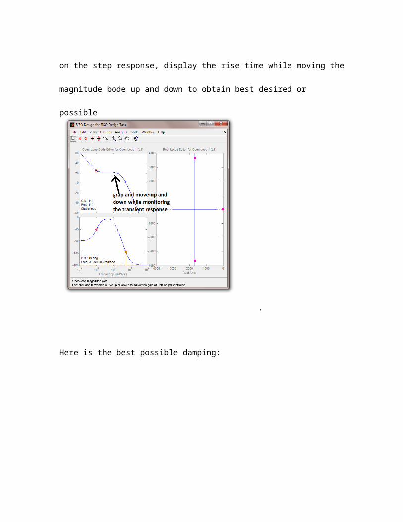
on the step response, display the rise time while moving the magnitude bode up and down
to obtain best desired or possible
.
Here is the best possible damping:
Step Response
Time (sec)
Ampl
itude
0 0.05 0.1 0.150
0.2
0.4
0.6
0.8
1
1.2
1.4From: Step To: Transfer Fcn
Rise time is: 0.58 ms (Excellent )
What is the big problem here ? ---------------------------------
- next, save the controller parameters and update the Simulink block
Here are the new values for Kp and Kd
Observations:
2- Set up the controller and a PI compensator
repeat the steps above, but this time with Kd set to zero.
Gp(s)
2.718e09
s +3408 .26s+1203982 .082Step ScopePI Controller
PID 1/s
The resulting system’s response is:
Step Response
Time (sec)
Ampl
itude
0 0.005 0.01 0.015 0.02 0.025 0.03 0.0350
0.2
0.4
0.6
0.8
1
1.2
1.4From: Step To: Transfer Fcn
System: Closed Loop from Step to Transfer FcnI/O: Step to Transfer FcnRise Time (sec): 0.00834
The controller parameters are:
Observations on the PD and the PI compensation results:
3- PID tuning
repeat the steps above but this time with a PID controller
Gp(s)
2.718e09
s +3408 .26s+1203982 .082Step ScopePID Controller
PID 1/s
all parameters are set to 1
The acceptable response is:
Step Response
Time (sec)
Ampl
itude
0 0.02 0.04 0.06 0.08 0.1 0.120
0.2
0.4
0.6
0.8
1
1.2
1.4System: Closed Loop from Step to Transfer FcnI/O: Step to Transfer FcnPeak amplitude: 1.05Overshoot (%): 4.54At time (sec): 0.0104
From: Step To: Transfer Fcn
System: Closed Loop from Step to Transfer FcnI/O: Step to Transfer FcnRise Time (sec): 0.00412
it was not possible to also meet the settling time requirement.
Observations about the overall result and how the solution is not unique.