Design of an optimal control for an autonomous mobile robot · DESIGN OF AN OPTIMAL CONTROL FOR AN...

INSTRUMENTACION REVISTA MEXICANA DE FISICA 57 (1) 75–83 FEBRERO 2011

Design of an optimal control for an autonomous mobile robot

E.M. Gutierrez-Arias, J.E. Flores-Mena, M.M. Morin-Castillo, and H. Suarez-RamırezFacultad de Ciencias de la Electronica, Benemerita Universidad Autonoma de Puebla,

Av. San Claudio y 18 Sur, Ciudad Universitaria, Colonia Jardines de San Manuel, Puebla, Pue., 72570, Mexico,e-mails: [email protected], [email protected], [email protected], [email protected]

Recibido el 18 de enero de 2010; aceptado el 11 de noviembre de 2010

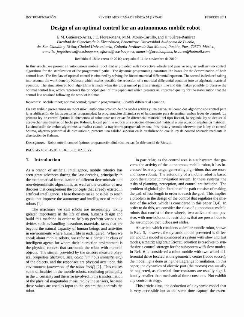
In this article, we present an autonomous mobile robot that is provided with two active wheels and passive one, as well as two controlalgorithms for the stabilization of the programmed paths. The dynamic programming constitute the bases for the determination of bothcontrol laws. The first law of optimal control is obtained by solving the Ricatti matricial differential equation. The second is deduced takinginto account the work done by Kalman, which makes possible the reduction of a matricial differential equation into an algebraic matricialequation. The simulation of both algorithms is made when the programmed path is a straight line and this makes possible to observe theoptimal control law, which represents the principal goal of this paper, and which presents an improved quality for the stabilization that thecontrol law obtained following the work of Kalman.

Keywords: Mobile robot; optimal control; dynamic programming; Ricatti’s differential equation.

En este trabajo presentamos un robot movil autonomo provisto de dos ruedas activas y una pasiva, ası como dos algoritmos de control parala estabilizacion de las trayectorias programadas; la programacion dinamica es el fundamento para determinar ambas leyes de control. Laprimera ley de controloptimo la obtenemos al solucionar una ecuacion diferencial matricial del tipo Riccati, la segunda ley se deduce alaprovechar una disertacion hecha por Kalman, la cual permite reducir una ecuacion diferencial matricial a una ecuacion algebraica matricial.La simulacion de ambos algoritmos se realiza cuando la trayectoria programada es una lınea recta y permite observar que la ley de controloptimo, objetivo primordial de este artıculo, presenta una calidad superior en la estabilizacion que la ley de control obtenida mediante ladisertacion de Kalman.

Descriptores: Robot movil; control optimo; programacion dinamica; ecuacion diferencial de Riccati.

PACS: 45.40.-f; 45.80.+r; 46.15.Cc; 02.30.Yy.

1. Introduction

As a branch of artificial intelligence, mobile robotics hasseen great advances during the last decades, principally inthe mathematical formalization of different deterministic andnon-deterministic algorithms, as well as the creation of newtheories that complement the concepts that already existed inartificial intelligence. These theories make possible to reachgoals that improve the autonomy and intelligence of mobilerobots [1].

The machines we call robots are increasingly takinggreater importance in the life of man, humans design andbuild this machine in order to help us perform various ac-tivities such as handling hazardous materials, tasks that arebeyond the natural capacity of human beings and activitiesin environments where human life is endangered. When wespeak about mobile robots, we refer to a particular class ofintelligent agents for whom their interaction environment isthe physical context that surrounds the robot with materialobjects. The stimuli provided by the sensors measure phys-ical properties (distance, size, color, luminous intensity, etc.)of the objects, and the responses are physical acts upon thisenvironment (movement of the robot itself) [2]. This causessome difficulties in the mobile robots, consisting principallyin the uncertainty and the error involved in the transformationof the physical magnitudes measured by the sensors, becausethese values are used as input to the system that controls therobot.

In particular, as the control area is a subsystem that go-verns the activity of the autonomous mobile robot, it has in-creased its study range, generating algorithms that are moreand more robust. The autonomy of a mobile robot is basedupon the automatic navigation system. In these systems, thetasks of planning, perception, and control are included. Theproblem of global planification of the path consists of makingthe path of less length in order to reach the goal. This impliesa problem in the design of the control that regulates the mis-sion of the robot, which is considered in this paper [3,4]. Inorder to do this, we consider the class of autonomous mobilerobots that consist of three wheels, two active and one pas-sive, with non-holonomic restrictions, that are present due tothe assumption that it does not slides.

An article which considers a similar mobile robot, shownin Ref. 5, however, the dynamic model presented is differ-ent and this model is considered a system with slow and fastmodes, a matrix algebraic Riccati equation is resolves to syn-thesize a control strategy for the subsystem with slow modes.In Ref. 6 is considered a robot mobile with two-wheel dif-ferential drive located at the geometric centre (robot soccer),the modeling is done using the Lagrange formulation. In thispaper, the dynamics of electric part (the motors) can usuallybe neglected, as electrical time constants are usually signif-icantly smaller than mechanical time constants. Not exhibitany control strategy.

This article aims, the deduction of a dynamic model thatis very accessible but at the same time capture the essen-

76 E.M. GUTIERREZ-ARIAS, J.E. FLORES-MENA, M.M. MORIN-CASTILLO, AND H. SUAREZ-RAMIREZ

tial nonlinearities such robots; synthesize two optimal controlstrategies to plan a robot path, considering a quadratic perfor-mance indicator. The first law to get when we solve a Riccatidifferential matrix equation, the second control law deducedfrom the previous work done by Kalman. The second controlstrategy we get it for comparison between the two and showthat the strategy obtained by solving the matrix differentialequation has a higher quality stabilization.

This paper is organized in the following way. Sec. 2 isdevoted to the statement of the control problem. In Sec. 3,the mathematical model of the mobile robot is deduced. InSec. 4, the programmed paths of the mobile robot is de-scribed, using the fact that every real path can be achievedas combinations of the programmed paths. In Sec. 5, thelinear equations of the state variables are considered for theprogrammed paths. In Sec. 6 and 7, the first and secondcontrol laws are obtained, respectively, as well as the solu-tion algorithms and their simulations. Finally, in Sec. 8, theconclusions obtained are presented.

2. Statement of the Problem

Let us consider the following controllable process:

y = f(y,u),u(·) ∈ U = u : u(t) ∈ Ω ⊆ Rr ,

(1)

wherey is thenth-dimensional vector that contains the statecoordinates of the system,u is the rth-dimensional vectorthat represents the input controls andf(y,u) belongs to theC2 class. The control is a vectorial function that is piece-wise continuous, and which for every instant of time, it takesits values from the convex, closed, and boundedΩ set. Letus assume that given some displacementyd(t) and a desiredcontrolud(t), the following equations are satisfied:

yd ≡ f(yd(t),ud(t)),u(.) ∈ U t ∈ [t0, t1).

(2)

Let there bem sensors that produce data about the actualmovement. After the processing of this data, it is possible tomake an estimate of the actual deviationsx(t) = y(t)−yd(t)and to form the control of the actor.

Let us use the following notation:

• ∆u = u− ud is the additional control,

• x = y−yd is the deviation respect to the desired move-ment,

• z = ϕ(y) − ϕ(yd) is the information vector that isreceived concerning the deviation.

The differential equations that govern the deviations

x(t)=y(t)−yd(t) for u(t) = ud(t), [t0, t1)

can be written as:

x = f(x, t), (3)

wheref(0, t) ≡ 0 for t ∈ [t0, t1) andx(t0) 6= 0. These equa-tions admit a trivial solution that corresponds to the desiredmovementyd(t) of the system.

Let us assume thatud(t) is located inside theΩ set fort ∈ [t0, t1) (this means that there still remain additional re-sources). For a given control strategyu = ud(t) + ∆u(z, t)where∆u is the additional control. Afterwards, the follow-ing linear equations of the deviations are obtained:

x = A(t)x + B(t)∆u, (4)

where

A(t) =∂f [yd(t),ud(t)]

∂y,

B(t) =∂f [yd(t),ud(t)]

∂u, (5)

and the linear model of measurement is

z = H(t)x detH 6= 0, (6)

where

H(t) =∂ϕ[(yd(t)]

∂y. (7)

Let us suppose that the perturbations upon the system andthe measurement errors are null. Almost without exception,there are initial perturbations that are presentx(t0) 6= 0 andthere is only a small number of cases in which for∆u ≡ 0,the conditionx(t) → 0 if t → ∞. Nevertheless, it is muchmore probable to have the case in which for∆u ≡ 0, theconditionx(t) 9 0 if t →∞ is satisfied.

This results into the stabilization problem; that is, withthe use of the information of the desired path, we have to de-

FIGURE 1. Autonomous Mobile Robot.

Rev. Mex. Fıs. 57 (1) (2011) 75–83

DESIGN OF AN OPTIMAL CONTROL FOR AN AUTONOMOUS MOBILE ROBOT 77

FIGURE 2. Diagram of the mobile robot.

termine a control∆u(z, t) such that the real deviations de-crease asymptotically. In this paper, it is assumed that wehave the exact and complete information of each one of thecoordinates [7].

3. Dynamic model of the mobile robot

The dynamic model of the mobile robot plays an importantrole in the simulation of the movement, the analysis of themechanic structure of the prototype, and in the design of thecontrol algorithms [8,9]. The autonomous mobile robot thatwas constructed, is shown in Fig. 1. As can be seen, theprototype consists of a straight, non-homogeneous cylinder,with two lateral wheels and one smaller that function as thesupport. The movement of the small wheel is not considered,due to the fact that its mass and size are small when comparedto the body of the robot.

For the construction of the dynamic model of the mobilerobot, we make the following considerations: a) The mobilerobot moves upon a plane; b) we suppose that the parts of themobile robot are rigid bodies; c) the movement of the smallwheel of support is not considered, which can be done be-cause the mass and size of the wheel are small in comparisonto those of the body of the robot; d) the velocities of the mo-bile robot are small, so that the viscous friction force can besafely ignored; e) the lateral wheels satisfy the non-slippingcondition; and f) the friction between the wheels and the flatsurface is such that it satisfies the condition of lateral non-slipping of the wheels.

Taking into account these considerations, the mobil robotconstructed was modeled using a straight cylinder and twolateral wheels with a straight cylinder form, as can be seenin the Figs. 2 and 3, where the mobile robot model is pre-sented, and which was used to obtain the dynamic model.The formulation employed to construct the dynamic modelis the Euler-Newton formulation, which consists of using thefollowing equation [10-12]:

FR = Macm (8)

and

τR =dLcm

dt, (9)

whereFR is the resultant force upon the massM of the bodyandacm is the acceleration of the mass center. On the otherhand, in Eq. (9)τR is the sum of external pairs andLcm isthe angular momentum around the axis that crosses the masscenter. Both of the equations are valid in an inertial systemwhich is assumed to be fixed on a flat surface upon which themobile robot, which is indicated by theX0

1 , X02 y X0

3 axes.Moreover, we consider a reference system that is fixed to therobot’s body, whose axes are denoted byXM

1 , XM2 y XM

3 ,and which are shown in Fig. 2.

Let C be a point that lies along theXM1 axis, and is lo-

cated at a distancec, with a position vectorrc, which willbe represented asrc = (x0

c1, x0c2, x

0c3)

T , and where the su-perindex states that the vector is expressed in the represen-tation of the inertial reference system. The representation ofthe vectorrc in the reference system that is fixed to the bodyhas components(xM

1c , xM2c , xM

3c )T .There is a very useful equation that shows the relationship

of the temporal variations that are measured in the two refer-ence systems, on inertial and the other fixed on the movingbody (which is denoted with an asterisk), which is

dBdt

=d∗Bdt

+ ω ×B, (10)

whereω is the angular velocity of the fixed system respectto the inertial system. Considering the pointC with positionvectorrc = R + C, whereR = (x0

1, x02, x

03)

T is the vectorthat goes from the origin of the inertial reference system tothe origin of the reference system that is fixed to the bodyandC = (c0

1, c02, c

03)

T is the vector that goes from the originof the reference system fixed to the body up to the pointC,using the Eq. (10), then the velocity of the pointC is givenby

x0

c1

x0c2

x0c3

=

v cos θ − ωc sin θ−v sin θ + ωc cos θ

0

, (11)

wherev =√

(x01)2 + (x0

2)2 andθ = ω is the translation ve-locity of the origin of the mobile reference system and theangular velocity around theX0

3 axis, respectively.The velocities of the centers of the wheels are obtained

by using the Eq. (10), so for the left and right wheels, weobtain

xM

l1

xMl2

xMl3

=

xM1 − aωxM

2

0

, (12)

and

xMr1

xMr2

xMr3

=

xM1 + aωxM

2

0

, (13)

Rev. Mex. Fıs. 57 (1) (2011) 75–83


respectively. In these expressions,a is the distance that liesbetween the origin of the system fixed to the body to that ofthe center of the wheel. These velocities have been calculatedfrom the representation of the reference system that is fixedto the body to keep simple the expression.

In order to calculate the acceleration, the Eq. (10) is used,applying it twice in order to obtain the equation of the secondderivative. The acceleration of a pointC that lies upon theXM

1 is given by the following equation

xMc1

xMc2

xMc3

=

xM1 − cθ2

xM2 + cθ

0

. (14)

The acceleration of the pointC is expressed in the represen-tation of the system fixed to the body. Following the sameprocedure, the acceleration at the center of the left and rightwheels are given by the following equations:

xMl1

xMl2

xMl3

=

xM1 − aθ

xM2 − aθ2

0

, (15)

and

xMr1

xMr2

xMr3

=

xM1 + aθ

xM2 + aθ2

0

, (16)

respectively.Taking into account the constriction relationships, let us

assume that the wheels satisfy the rolling and non-slippingconditions. (that no lateral slipping occurs in the wheels).The rolling condition is established using the following equa-tions

Vl = rφl, (17)

Vr = rφr, (18)

whereVl = xMl1 andVr = xM

r1 . With the help of these ex-pressions, it is possible to write down the first coordinate ofthe vectorial equations in the following manner (12), (13)

Vl = v − aω, (19)

Vr = v + aω, (20)

sincexM1 = v. The angular accelerations of the wheels of the

mobile robot are obtained by differentiating respect to timethe Eqs. (19) and (20). Thus,

αl =1r(xM

1 − aθ), (21)

αr =1r(xM

1 + aθ), (22)

whereαl = φl, αr = φr y r is the radius of the wheels.The no-slip lateral condition of the wheels is established

by requiring that the following conditions are satisfied:

xMl2 = xM

r2 = xM2 = 0. (23)

FIGURE 3. Free-Body Diagram.

Moreover, the transformation equations for the velocitiesof the origin of the fixed reference system to the inertial sys-tem, can be written in the following way:

xM1

xM2

xM3

=

cos θ sin θ 0− sin θ cos θ 0

0 0 1

x01

x02

x03

. (24)

Now, by considering the second component of the expres-sion (24) and taking into account the expression (23), the fol-lowing equation is obtained:

xM2 = −x0

1 sin θ + x02 cos θ = 0, (25)

and by differentiating respect to time, then

xM2 = 0. (26)

Using the free-body diagram of Fig. 3, it is possible towrite for every mobile part of the robot the Eq. (8). For thebody of the robot, the Eq. (14) has been used in Eq. (8),wherec = −b, so

(F′l + F

′r

R′l + R

′r

)= mb

(xM

1 + bθ2

xM2 − bθ

), (27)

wheremb is the mass of the body of the robot andb is thedistance between the system that is fixed on the body up tothe robot’s mass center. For the left wheel, it is possible towrite the Eq. (8) as

(Fl − F

′l

Rl −R′l

)= mwl

(xM

1 − aθ

xM2 − aθ2

). (28)

In this expression,mwl is the mass of the left wheel. Mean-while, for the right wheel, Eq. (8) can be rewritten as

(Fr − F

′r

Rr −R′r

)= mwr

(xM

1 + aθ

xM2 + aθ2

). (29)

In this expression,mwr is the mass of the right wheel.Adding the corresponding members of Eqs (27), (28),and (29), then

(Fl + Fr

Rl + Rr

)=

(mbx

M1 + mbbθ

2 + 2mwxM1

mbxM2 −mbbθ + 2mwxM

2

), (30)

Rev. Mex. Fıs. 57 (1) (2011) 75–83


where it has been considered that the masses of the wheelsare equal,mwl = mwr = mw.

In order to finish the dynamic model of the mobile robot,it is necessary to apply the second equation of the Euler-Newton formulation to the robot model shown in Figs. 2and 3. Equation (9), can be rewritten as:

τR = ICM · dω

dt+ mrCM × dvCM

dt. (31)

In order to obtain the equation that completes the dynamicmodel of the mobile robot, we employed the same plan thatproduced the Eqs. (30). Considering the free-body diagramof Fig. 3, and using Eq. (31) for the robot’s body and the twowheels, and adding the corresponding sides of the resultantequations, then

a(Fr − Fl) = (I3c + 2I3w

+2mwa2 + mbb2)θ −mbbx

M2 . (32)

In this expression,I3c is the momentum of inertia along theaxis that goes through the mass center, which is the robot’scenter, and which is parallel toXM

3 , while I3w is the mo-mentum of inertia along the axis that goes through the masscenter of a wheel and that is parallel to theXM

3 axis.Therefore, to obtain the relationship between the pairs ap-

plied by the engines upon the wheels (τl , τr) and the tractionforces that are produced upon the wheels (Fl, Fr), we applyfor each one of the wheels the expression

∑i τi = Iα, where

the sum of the applied pairs are those who are responsible tothe rolling of the wheel with an angular accelerationα aroundthe rotation axis with a momentum of inertiaI. Consideringthe free-body diagram of Fig. 3 and the angular accelerationsof the wheels in the expressions (21) and (22), then

Fl =1r

[τl − I2w

r

(xM

1 − aθ)]

, (33)

Fr =1r

[τr − I2w

r

(xM

1 + aθ)]

, (34)

whereI2w is the momentum of inertia respect to the axis thatpasses through the axis that connects the two wheels.

Substituting the equations (33) and (34), in the first com-ponent of the expressions (28) and (32), then

(τr + τl)r

=(

mb + 2mw +2I2w

r2

)xM

1 + mbbθ2, (35)

a(τr − τl)r

=(

I3c + mbb2

+ 2I3w + 2mwa2 +2a2

r2I2w

)θ, (36)

respectively.The model of the motor which is being considered is the

following one [13]:

τi = χui − σφi, i = l, r, (37)

TABLE I. Programmed trajectories of horizontal and vertical lines.

Trajectory x0dc1 x0d

c2 θd vd ωd

1. horizontal line v0t + ξ0 0 0 v0 0

negative sense

2. horizontal line v0t + ξ0 0 π v0 0

positive sense

3. vertical line 0 v0t + η0π2

v0 0

negative sense

4. vertical line 0 v0t + η0 −π2

v0 0

positive sense

whereui is the potential difference applied to the enginei,φi is the angular velocity at which the engine’s axisi rotates,χ is the ratio that exists between the constant electromotiveforce and the electric resistance of the engine andσ is the ra-tio between the counter-electromotive force and the electricresistance. Considering this expression and using (17)-(20),then

(τr + τl) = χ(ur + ul)− σ2v

r, (38)

(τr − τl) = χ(ur − ul)− σ2aω

r. (39)

Finally, substituting Eqs. (38) and (39) in Eqs. (35)and (36) and by using Eq. (11), but withc = h, and bycombining them, we obtain the dynamic model

x0c1 = v cos θ − hω sin θ,

x0c2 = v sin θ + hω cos θ,

θ = ω,

J1v = −mbbω2 − 2σ

r2 v + χr (ur + ul),

J2ω = 2a2σr2 ω + aχ

r (ur − ul).

(40)

where

J1 = mb + 2mw + 2I2w/r2

and

J2 = I3c + 2I3w + 2mwa2 + mbb2 + 2a2I2w/r2.

The expression of the dynamic model, Eq. (40) is a non-linear system of five differential equations that have two con-trol variablesur y ul.

4. Programmed Paths

The stationary programmed pathsyd(t), are determined froma specific activity of the robot, and they are given in such a

Rev. Mex. Fıs. 57 (1) (2011) 75–83


FIGURE 4. Training Board of the Mobile Robot

way that this activity will be regulated by the desired move-ment.

It is possible to approximate any assigned activity bycombinations of horizontal o vertical straight lines and bysemicircles. We will make eight possible configurations (ascan be seenin Fig. 4).

We show the set of desired paths in Table I, where themovement is done along a segment of a line parallel to the(X0

1 axis or to theX02 axis).

In the case in which the robot goes along a horizontal orvertical straight line, as can be seen in Table I, it is assumedthat there will be no angular movement(ωd = 0). Thoseequations that satisfy this set of conditions is said to be in anequilibrium state.

If the robot moves along a segment of a circle with diam-eterR that is centered on one of the corners of the trainingboard, and if we consider this corner and the configuration ofthe training board, we have four quadrants that are countedcounterclockwise, dividing the circle into four equal semicir-cles. In this situation, it is possible to describe eight possibleconfigurations. Moreover, the set of solutions for the desiredpath results from considering that the robot describes a semi-circular movement, so we assume a constant angular move-ment. The velocity and the angle are given from this angulardisplacement, as well as the position coordinates.

5. Linear Equations in the Deviations

If ud(t) is a nominal entry to the system that is described byEqs. (40) andyd(t) is a nominal path of this system, then it ispossible to find approximations to the neighboring solutionsfor small deviations from the initial state and for the entry.Let us suppose that the system is closed for nominal condi-tions, which implies thatu(t) andy(t) will slightly deviatefrom ud(t) andyd(t).

The linear system for the horizontal line in the positivesense is given by:

TABLE II. Numerical values of system’s parameters.

Variable Value Description

v0 1.5 wanted speed, in meters/seconds

a 0.40 Distance between wheels, in meters

b 0.08 Distance between masses center and

the axis of wheels, in meters

h 0.10 Distance between the wheels and

the array of infrared sensors, in meters

m 4.5 Mass of robot, in kilograms

r 0.08 Radius of wheels, in meters

x0c1 = −v,

x0c2 = −v0θ − hω,

θ = ω,

v = − 2σr2J1

v + χrJ1

(ur + ul),

ω = 2a2σr2J2

ω + aχrJ2

(ur − ul).

(41)

Considering that the desired path is a semicircle, then weobtain the eight systems for the linear deviations, substitutingin the following system each one of the desired movements(in this caseeach system depends onθd), we present one ofthese:

x0c1 = − (

v0 sen θd + hω0 cos θd)θ

+ v cos θd − ωh sen θd,

x0c2 =

(−v0 cos θd − hω0 sen θd)θ

+v sen θd + ωh cos θd,

θ = ω,

v = − 2σr2J1

v − 2bω0ωmbJ1

+ χrJ1

(ur + ul),

ω = 2a2σr2J2

ω + aχrJ2

(ur − ul).

(42)

6. First law of optimal control and solution al-gorithm

Considering the system

x = Ax(t) + Bu(t), (43)

and the stabilization quality functional is given by

G(x,u) =

∞∫

0

(xT (t)G(t)x(t) + uT (t)N(t)u(t))dt. (44)

Rev. Mex. Fıs. 57 (1) (2011) 75–83


FIGURE 5. Diagram of flux to solve the Riccati’s differential ma-tricial equation.

The programmed path is considered as a straight line inthe negative direction (Table I)

x0dc1

x0dc2

θd

vd

ωd

=

v0t + ξ0

0

π

v0

0

. (45)

The matricesA,B of the system (43) are obtained ac-cording to the values of the parameters of the Table II and aredescribed below:

A =

0 0 0 −1 00 0 −1.5 0 −0.10 0 0 0 10 0 0 0.625 00 0 0 0 0.3923

, (46)

B =

0 00 00 0

0.0278 00 0.1744

. (47)

Using the dynamic programming and by consideringBellman’s function,w(x, t) = x(t)L(t)x(t), we obtain Ric-catti’s matricial differential equation [14,15].

L = LBBTL − 2AL −G con L(t1) = 0. (48)

For a given instantt1, we proceed to solve this system in theinverse time as a system with initial conditions using a vari-able exchangeτ = t − t1, so that the system (48), which isa non-linear system with final conditions, is transformed to asystem with initial conditions.

Afterwards, with the use of polynomials, it is possible toobtain an approximation of each one of the matrix elementsL(t). Since these functions are written in the inverse time,it is necessary to return to the direct time, obtaining all thematrix elementsL(t), and thus, the optimal control is writtenas

u = −N−1BTL(t)x(t). (49)

Finally, we substitute this control into the system

x = A(t)x + B(t)u,

and by solving forx=(A − BBTL)x, we simulate the be-havior of the state variables.

FIGURE 6. Behavior of the state variables when the control con-sidersL(t)

Rev. Mex. Fıs. 57 (1) (2011) 75–83


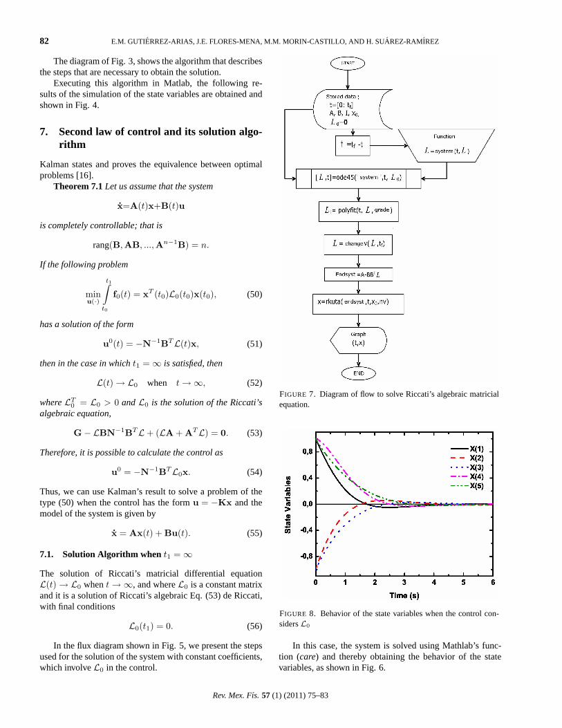
The diagram of Fig. 3, shows the algorithm that describesthe steps that are necessary to obtain the solution.

Executing this algorithm in Matlab, the following re-sults of the simulation of the state variables are obtained andshown in Fig. 4.

7. Second law of control and its solution algo-rithm

Kalman states and proves the equivalence between optimalproblems [16].

Theorem 7.1Let us assume that the system

x=A(t)x+B(t)u

is completely controllable; that is

rang(B,AB, ...,An−1B) = n.

If the following problem

minu(·)

t1∫

t0

f0(t) = xT (t0)L0(t0)x(t0), (50)

has a solution of the form

u0(t) = −N−1BTL(t)x, (51)

then in the case in whicht1 = ∞ is satisfied, then

L(t) → L0 when t →∞, (52)

whereLT0 = L0 > 0 andL0 is the solution of the Riccati’s

algebraic equation,

G− LBN−1BTL+ (LA + ATL) = 0. (53)

Therefore, it is possible to calculate the control as

u0 = −N−1BTL0x. (54)

Thus, we can use Kalman’s result to solve a problem of thetype (50) when the control has the formu = −Kx and themodel of the system is given by

x = Ax(t) + Bu(t). (55)

7.1. Solution Algorithm when t1 = ∞The solution of Riccati’s matricial differential equationL(t) → L0 whent →∞, and whereL0 is a constant matrixand it is a solution of Riccati’s algebraic Eq. (53) de Riccati,with final conditions

L0(t1) = 0. (56)

In the flux diagram shown in Fig. 5, we present the stepsused for the solution of the system with constant coefficients,which involveL0 in the control.

FIGURE 7. Diagram of flow to solve Riccati’s algebraic matricialequation.

FIGURE 8. Behavior of the state variables when the control con-sidersL0

In this case, the system is solved using Mathlab’s func-tion (care) and thereby obtaining the behavior of the statevariables, as shown in Fig. 6.

Rev. Mex. Fıs. 57 (1) (2011) 75–83


8. Conclusions

We obtained the movement Eqs. (40) of the mobile robotfor a horizontal straight line in the positive sense, we wrotedown the deviations linear system (41), and used this sys-tem to deduce both of the control laws. Using the dynamicprogramming as a basis, we obtained the first optimal con-trol law (49) by solving Riccati’s matricial differential equa-tion (48), and the stabilization time in the simulation is quiteacceptable, because by using the Kalman’s work, we have thesecond control law (54) when we solve Riccati’s matricial al-

gebraic equation (53), simplifying the calculations done inthis equation. Nevertheless, the stabilization time increasessignificantly, as can be seen in Fig. 6. A future paper willconsist of determining a control law when the programmedpath is a semicircle.

Acknowledgments

The authors are grateful for the financial support given byCONACyT of Mexico. JEFM is grateful for the support givenby VIEP-BUAP (project 7-ING-2009)

1. A. Ollero Baturone,Robotica Manipuladores y Robots Moviles(Marcobombo, 2001).

2. R. Siegwart and I.R. Nourbakhsh,Introduction to AutonomousMobile Robots(2004).

3. D.E. Kirk, Optimal Control Theory An Introduction(Printice-Hall, 1970).

4. G. Knowles,An Introduction to Applied Optimal Control(NewYork and London Academic Press, 1981).

5. A. Hemani, M.G. Mehrabi, and R.M.H. ChengAutomatice28(1991) 383.

6. G. Klancar, B. Zupancic, R. KarbaModelling and simulationof a group of mobile robots(Simulation Modelling Practice andTheory 15, ELSEVIER, 2007). pp. 647.

7. V.V. Alexandrov et al.,Introduction to Control of DynamicSystems1a ed. (Benemerita Universidad Autonoma de Puebla,2009).

8. M.R.M. Crespo da Silva,Intermediate Dynamics(McGraw-Hill, 2004).

9. Jean Jaques E. Slotine and Li. Weiping,Applied NonlinearControl (Pearson Education, Republic of China, 2004).

10. F.C. Moon,Applied Dynamics(John Wiley & Sons, Inc., 1998).

11. K.R. Symon,Mecanica2da ed. (Addison-Wesley, 1970).

12. J. Angeles, Fundamentals of Robotic Mechanical Systems(Springer-Verlag, 1997).

13. J. Jones and A.M. Flynn,Mobile Robots, Inspiration Implemen-tation (2da ed., Addison-Wesley, 2000).

14. R. Bellman,Mathematical Theory of Control Processesvol. I(New York and London, Academic Press, 1967).

15. R. Bellman,Mathematical Theory of Control Processes,vol. II(New York and London Academic Press, 1971).

16. R.E. Kalman,Contributions to the Theory of Optimal Control(Bulletin of Mexican Mathematic, 1960) P. 102.

Rev. Mex. Fıs. 57 (1) (2011) 75–83

Design of an optimal control for an autonomous mobile robot · DESIGN OF AN OPTIMAL CONTROL FOR AN...

Documents

Transcript of Design of an optimal control for an autonomous mobile robot · DESIGN OF AN OPTIMAL CONTROL FOR AN...