7630 Autonomous Robotics Mobile Robot Kinematicsdream.georgiatech-metz.fr/sites/default/files/3 -...

7630 – Autonomous Robotics Mobile Robot Kinematics

Motion Prediction

Odometry

Mobility Analysis

Based on material from R. Siegwart, M. Mason

Recommended Reading

• Introduction to Autonomous Mobile Robots, Siegwart, Nourbakhsh, Scaramuzza – http://www.mobilerobots.ethz.ch/

– Chapter 3

• Lecture from Matt Mason (CMU): – http://www.cs.cmu.edu/afs/cs/academic/class/16741-

s07/www/lecture5.pdf

http://www.mobilerobots.ethz.ch/

http://www.mobilerobots.ethz.ch/

http://www.cs.cmu.edu/afs/cs/academic/class/16741-s07/www/lecture5.pdf




http://www.amazon.com/gp/reader/0262015358/ref=sib_dp_pt

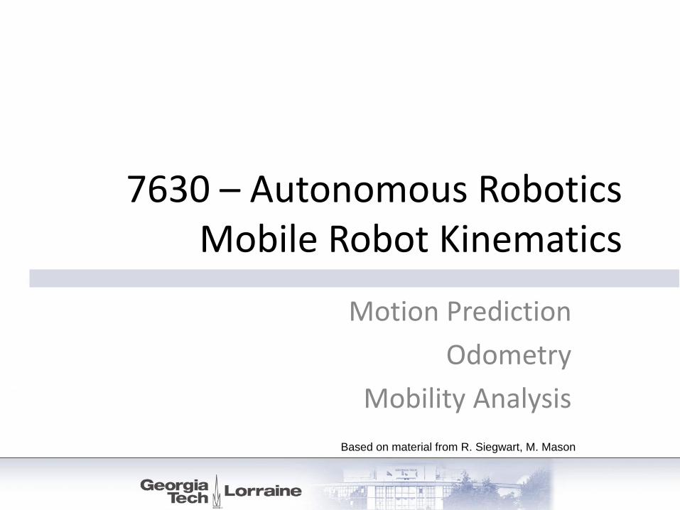
Athlete

Image source: NASA

DEFINITIONS

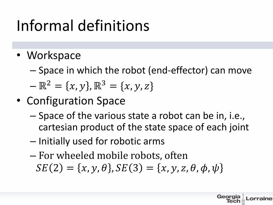
Informal definitions

• Workspace – Space in which the robot (end-effector) can move

– ℝ2 = 𝑥, 𝑦 ,ℝ3 = {𝑥, 𝑦, 𝑧}

• Configuration Space – Space of the various state a robot can be in, i.e.,

cartesian product of the state space of each joint

– Initially used for robotic arms

– For wheeled mobile robots, often 𝑆𝐸 2 = 𝑥, 𝑦, 𝜃 , 𝑆𝐸 3 = 𝑥, 𝑦, 𝑧, 𝜃, 𝜙, 𝜓

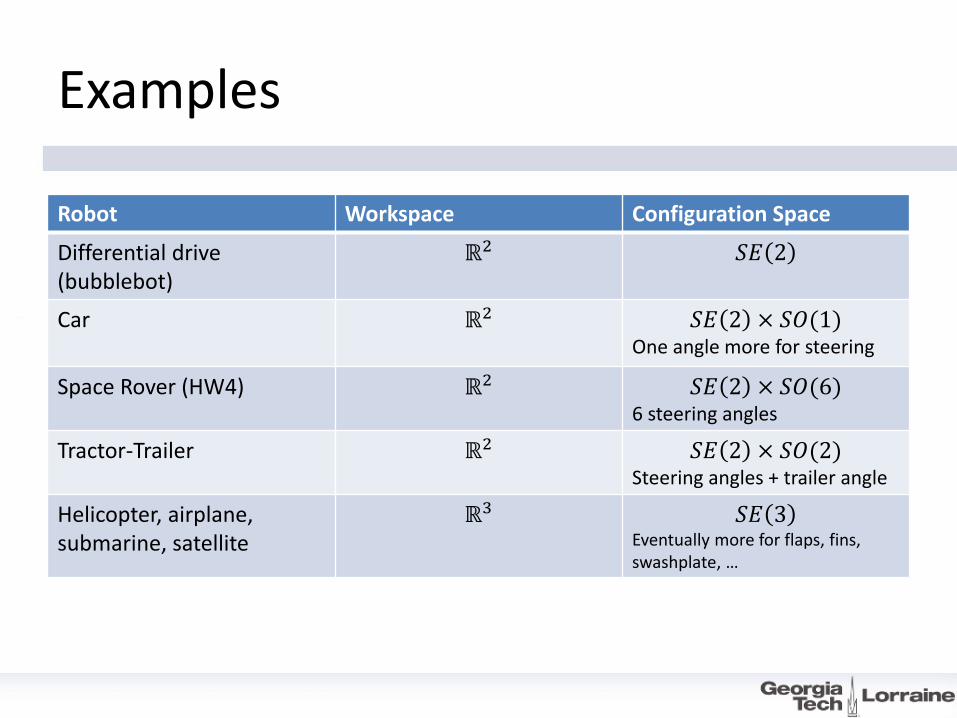
Examples

Robot Workspace Configuration Space

Differential drive (bubblebot)

ℝ2 𝑆𝐸 2

Car ℝ2

𝑆𝐸 2 × 𝑆𝑂(1) One angle more for steering

Space Rover (HW4) ℝ2 𝑆𝐸 2 × 𝑆𝑂(6) 6 steering angles

Tractor-Trailer ℝ2 𝑆𝐸 2 × 𝑆𝑂(2) Steering angles + trailer angle

Helicopter, airplane, submarine, satellite

ℝ3 𝑆𝐸 3 Eventually more for flaps, fins, swashplate, …

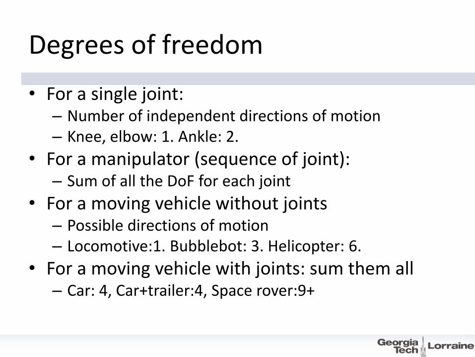
Degrees of freedom

• For a single joint: – Number of independent directions of motion – Knee, elbow: 1. Ankle: 2.

• For a manipulator (sequence of joint): – Sum of all the DoF for each joint

• For a moving vehicle without joints – Possible directions of motion – Locomotive:1. Bubblebot: 3. Helicopter: 6.

• For a moving vehicle with joints: sum them all – Car: 4, Car+trailer:4, Space rover:9+

MOBILITY ANALYSIS FOR WHEELS

For vehicles in the plane

© R. Siegwart, ETH Zurich - ASL

3 - Mobile Robot Kinematics 3

9 Introduction: Mobile Robot Kinematics

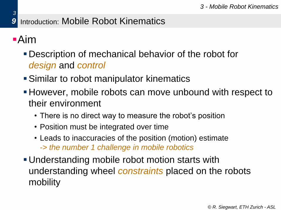
Aim

Description of mechanical behavior of the robot for

design and control

Similar to robot manipulator kinematics

However, mobile robots can move unbound with respect to

their environment

• There is no direct way to measure the robot’s position

• Position must be integrated over time

• Leads to inaccuracies of the position (motion) estimate

-> the number 1 challenge in mobile robotics

Understanding mobile robot motion starts with

understanding wheel constraints placed on the robots

mobility



10 Introduction: Kinematics Model

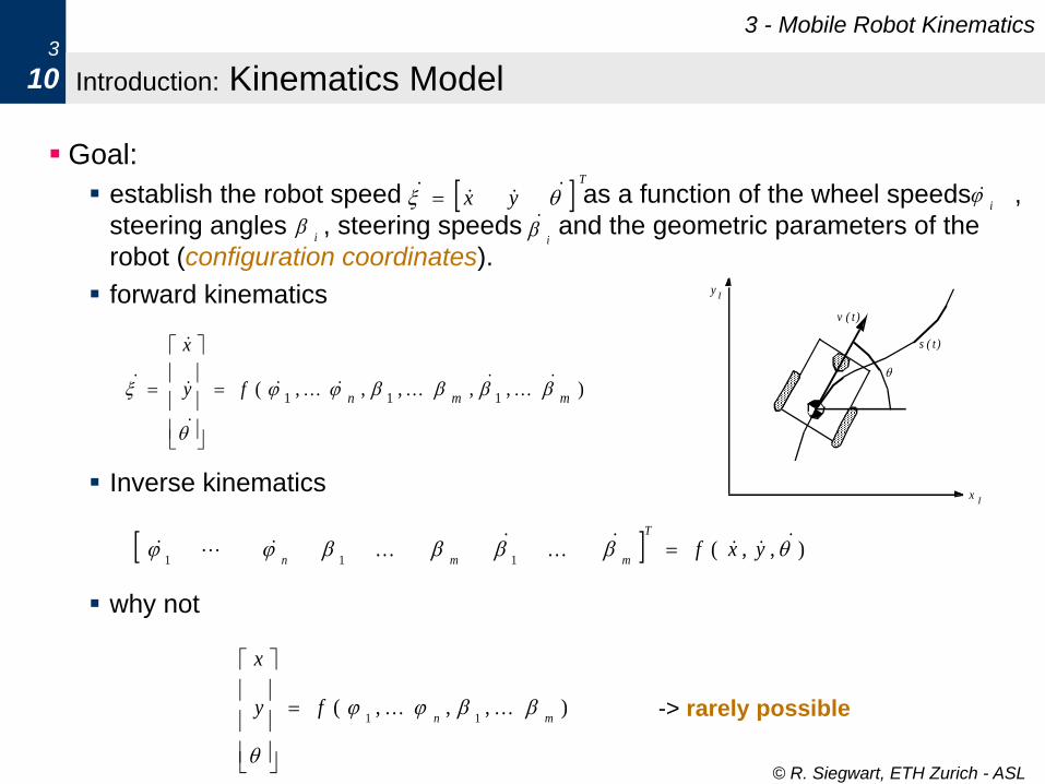
Goal:

establish the robot speed as a function of the wheel speeds ,

steering angles , steering speeds and the geometric parameters of the

robot (configuration coordinates).

forward kinematics

Inverse kinematics

why not

-> rarely possible

),,,,, (111 mmn

fy

x

T

yx

i

i

i

),, ( 111

yxfT

mmn

),,, (11 mn

fy

x

yI

xI

s ( t)

v ( t)



11

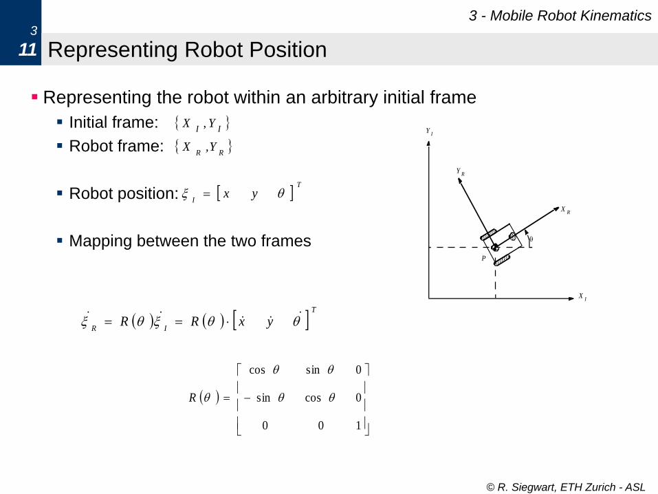
Representing the robot within an arbitrary initial frame

Initial frame:

Robot frame:

Robot position:

Mapping between the two frames

Representing Robot Position

T

Iyx

II

YX ,

RR

Y,X

100

0cossin

0sincos

R

T

IRyxRR

P

YR

XR

YI

XI



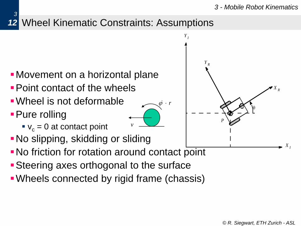
12 Wheel Kinematic Constraints: Assumptions

Movement on a horizontal plane

Point contact of the wheels

Wheel is not deformable

Pure rolling vc = 0 at contact point

No slipping, skidding or sliding

No friction for rotation around contact point

Steering axes orthogonal to the surface

Wheels connected by rigid frame (chassis)

r

v P

YR

XR

YI

XI



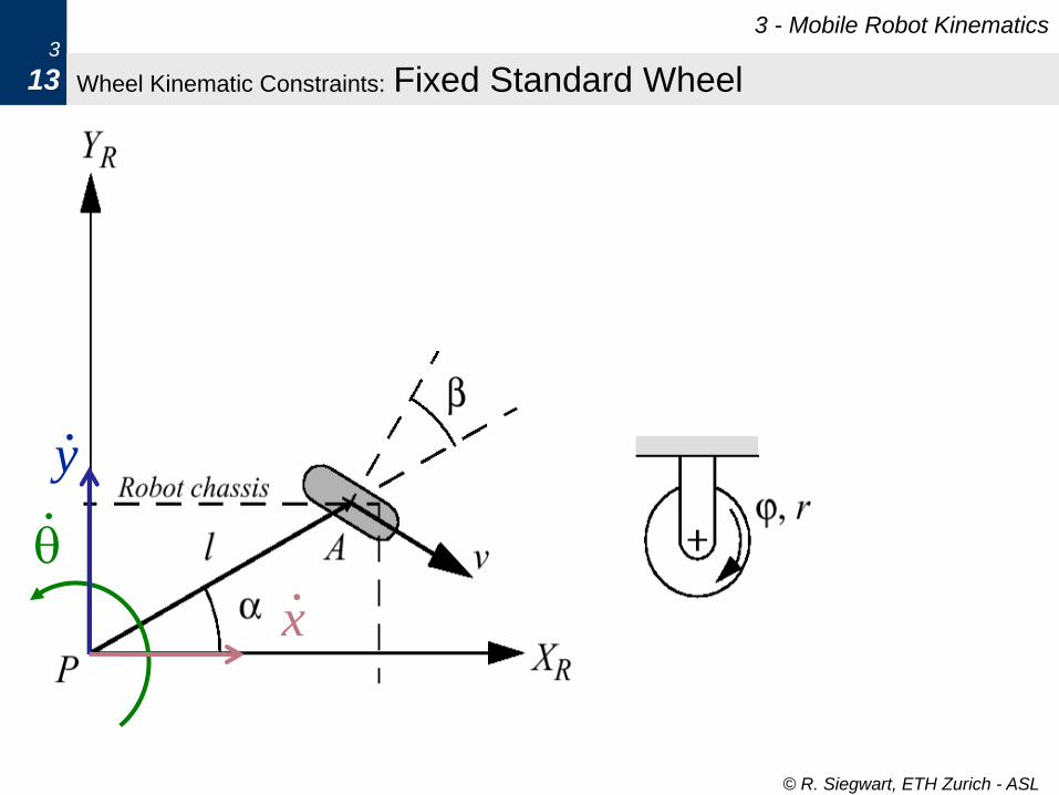
13 Wheel Kinematic Constraints: Fixed Standard Wheel

x .

y .

.

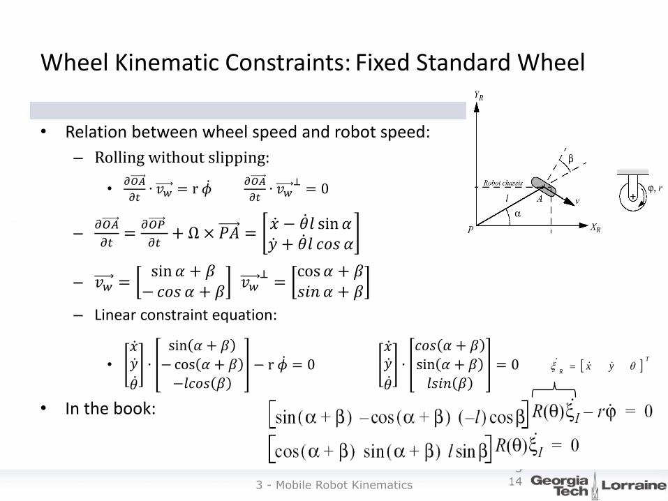
Wheel Kinematic Constraints: Fixed Standard Wheel

• Relation between wheel speed and robot speed:

– Rolling without slipping:

•𝜕𝑂𝐴

𝜕𝑡∙ 𝑣𝑤 = r 𝜙

𝜕𝑂𝐴

𝜕𝑡∙ 𝑣𝑤

⊥= 0

–𝜕𝑂𝐴

𝜕𝑡=

𝜕𝑂𝑃

𝜕𝑡+ Ω × 𝑃𝐴 =

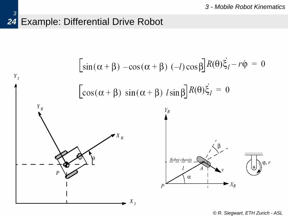
𝑥 − 𝜃 𝑙 sin 𝛼𝑦 + 𝜃 𝑙 𝑐𝑜𝑠 𝛼

– 𝑣𝑤 =sin𝛼 + 𝛽−𝑐𝑜𝑠 𝛼 + 𝛽

𝑣𝑤⊥=

cos𝛼 + 𝛽𝑠𝑖𝑛 𝛼 + 𝛽

– Linear constraint equation:

•

𝑥 𝑦

𝜃 ∙

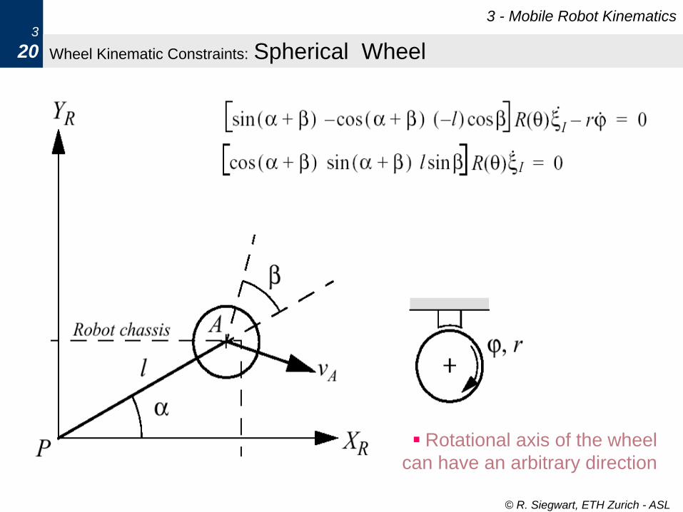
sin 𝛼 + 𝛽

−cos 𝛼 + 𝛽

−𝑙𝑐𝑜𝑠 𝛽

− r 𝜙 = 0 𝑥 𝑦

𝜃 ∙

𝑐𝑜𝑠 𝛼 + 𝛽

sin 𝛼 + 𝛽

𝑙𝑠𝑖𝑛 𝛽

= 0

• In the book:

3 - Mobile Robot Kinematics

3 14

T

Ryx


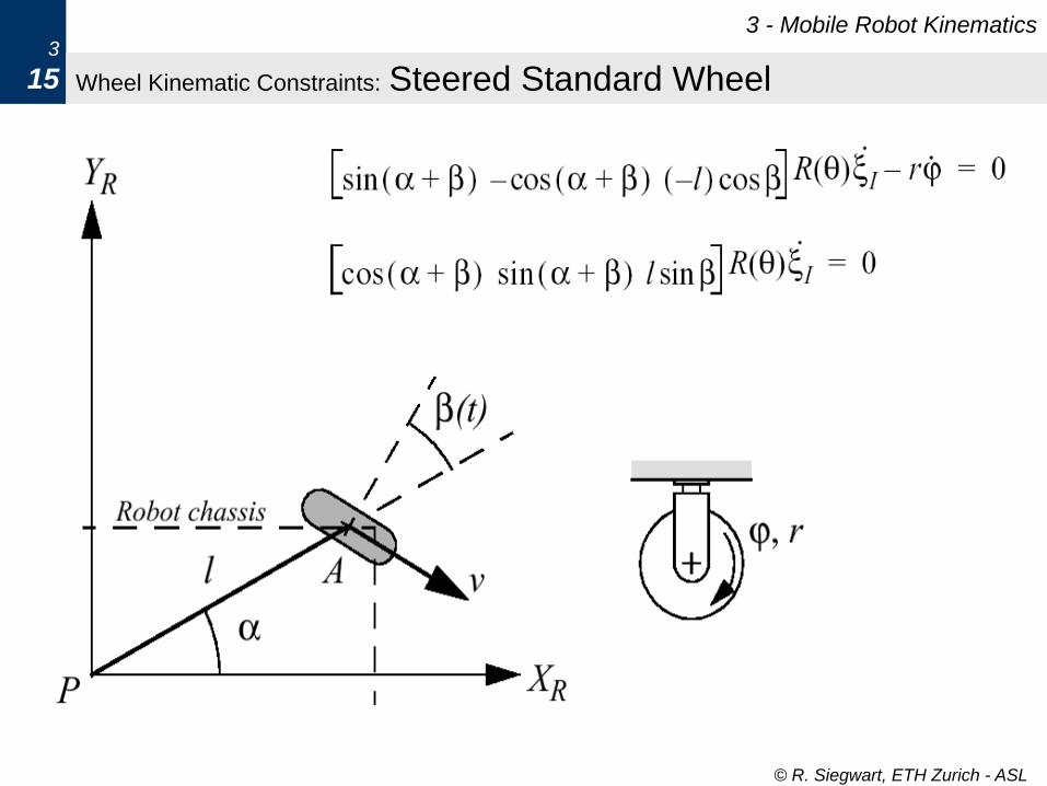
Wheel Kinematic Constraints: Steered Standard Wheel


15


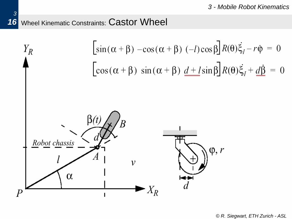
Wheel Kinematic Constraints: Castor Wheel


16

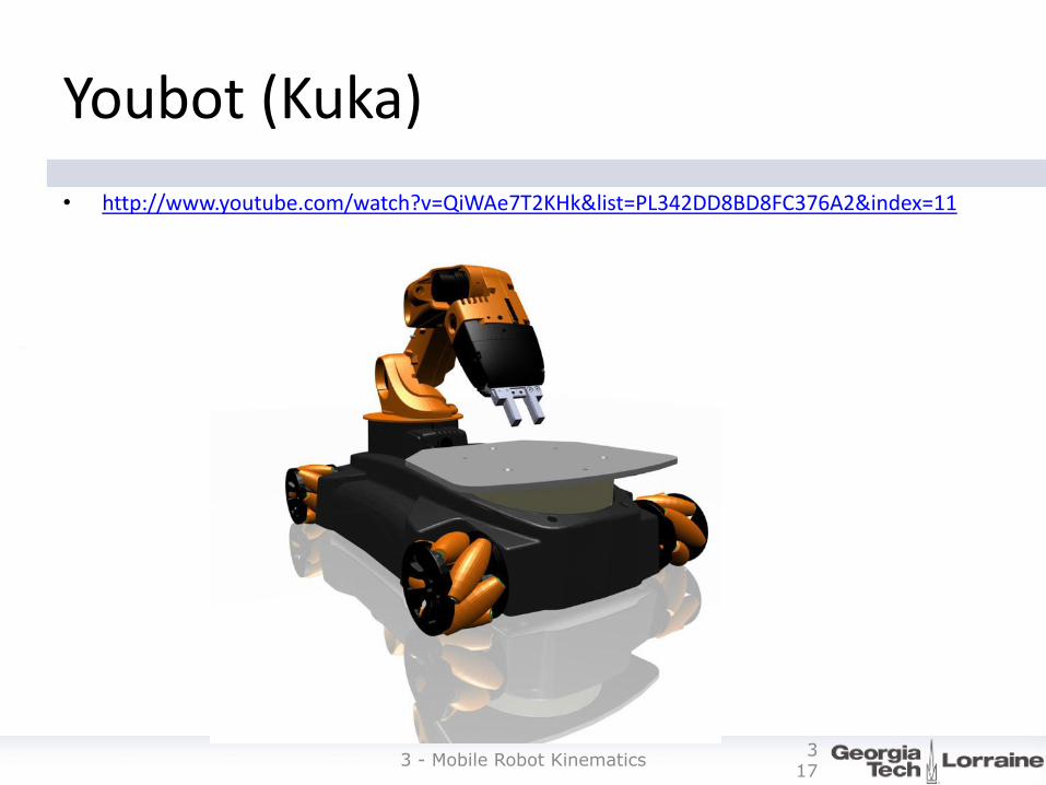
Youbot (Kuka)

• http://www.youtube.com/watch?v=QiWAe7T2KHk&list=PL342DD8BD8FC376A2&index=11


17

http://www.youtube.com/watch?v=QiWAe7T2KHk&list=PL342DD8BD8FC376A2&index=11


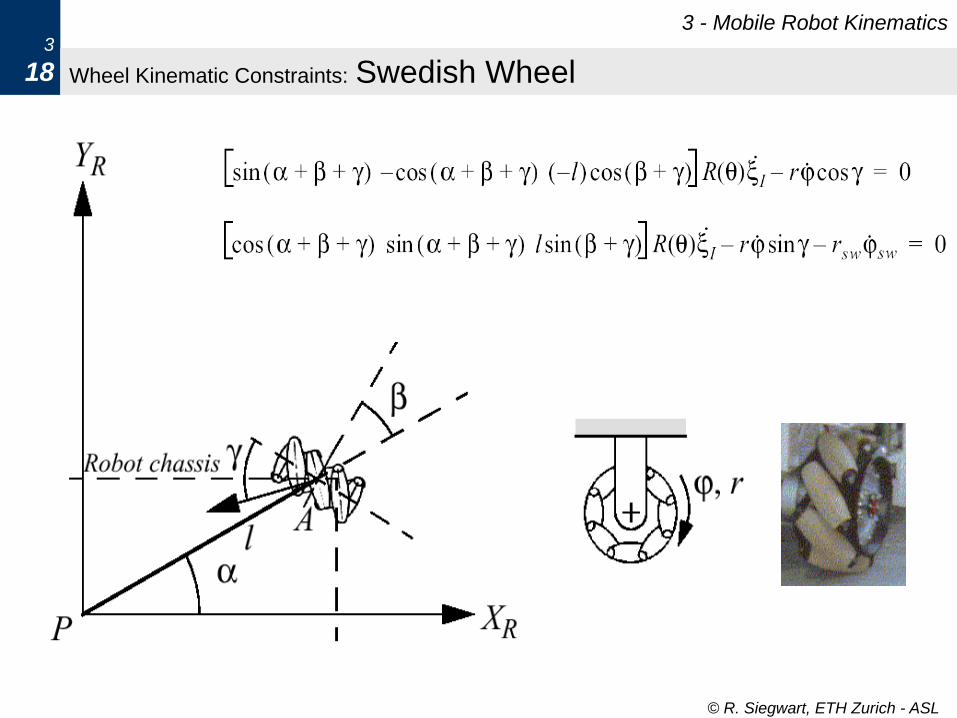
Wheel Kinematic Constraints: Swedish Wheel


18

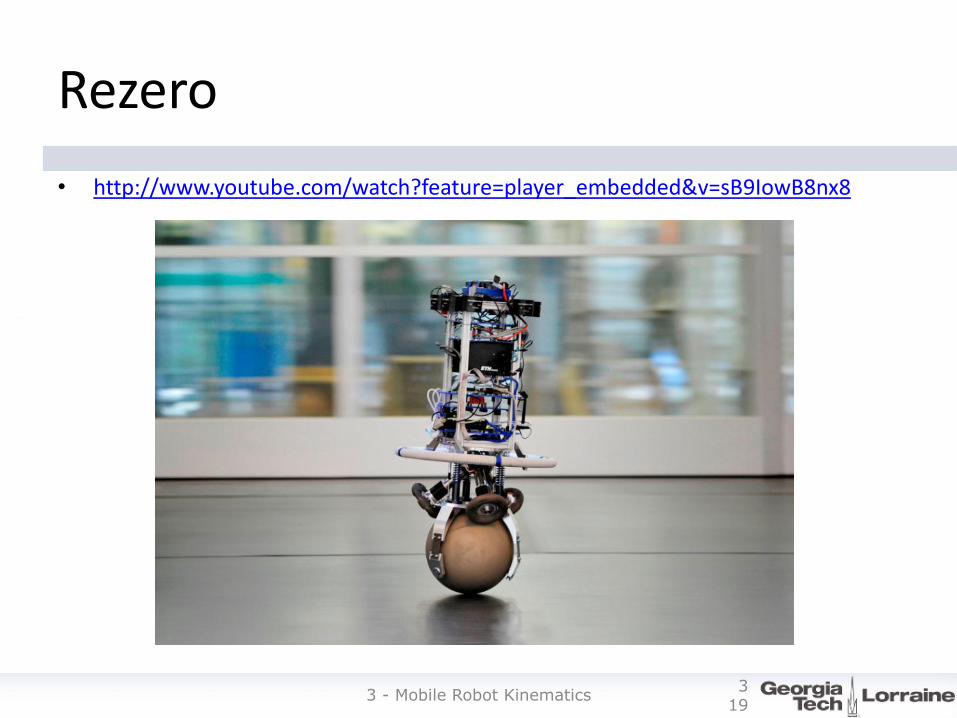
Rezero

• http://www.youtube.com/watch?feature=player_embedded&v=sB9IowB8nx8


19

http://www.youtube.com/watch?feature=player_embedded&v=sB9IowB8nx8








20 Wheel Kinematic Constraints: Spherical Wheel

Rotational axis of the wheel

can have an arbitrary direction

MOBILITY ANALYSIS FOR THE ROBOT

For vehicles in the plane



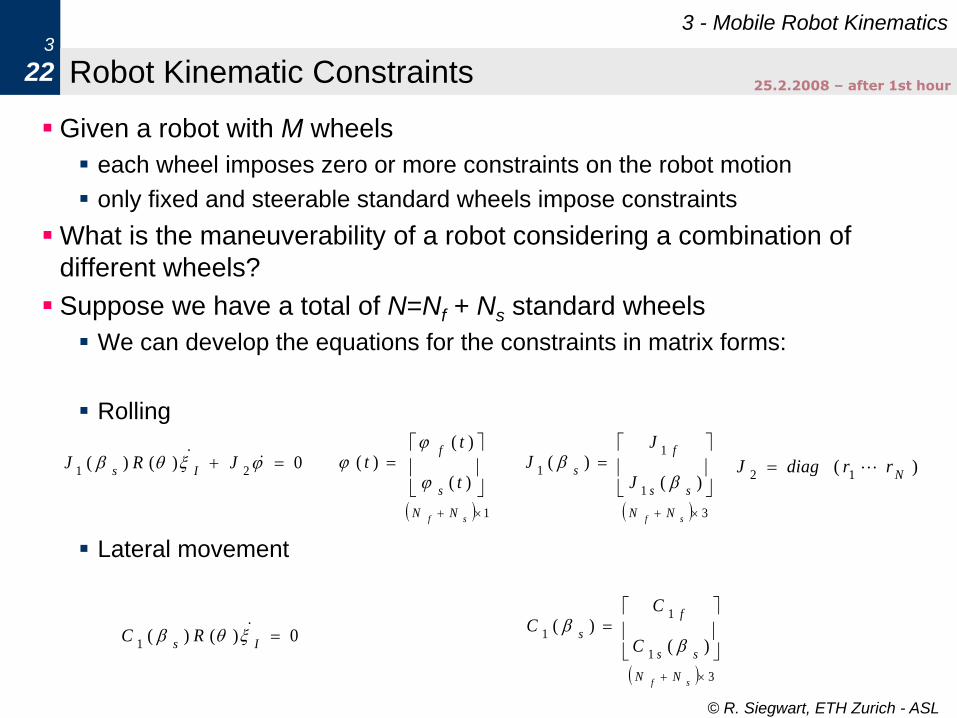
22 Robot Kinematic Constraints

Given a robot with M wheels

each wheel imposes zero or more constraints on the robot motion

only fixed and steerable standard wheels impose constraints

What is the maneuverability of a robot considering a combination of

different wheels?

Suppose we have a total of N=Nf + Ns standard wheels

We can develop the equations for the constraints in matrix forms:

Rolling

Lateral movement

1

)(

)()(

sfNN

s

f

t

tt

0)()(

21 JRJ

Is

3

1

1

1)(

)(

sfNN

ss

f

sJ

JJ

)(

12 NrrdiagJ

0)()(1

Is

RC

3

1

1

1)(

)(

sfNN

ss

f

sC

CC

25.2.2008 – after 1st hour

Example

• Kinematic of a differential drive

• Kinematic of the car

• Kinematic of a car with a trailer

– Why is it hard to reverse with a trailer?



24 Example: Differential Drive Robot

P

YR

XR

YI

XI



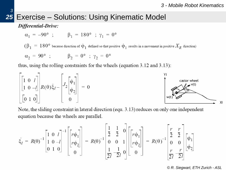
25 Exercise – Solutions: Using Kinematic Model

v(t)

w(t)

q

YI

XI

castor wheel



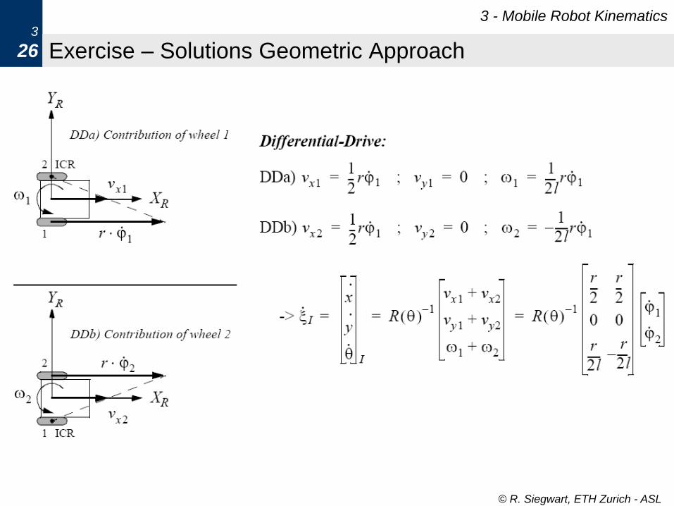
26 Exercise – Solutions Geometric Approach



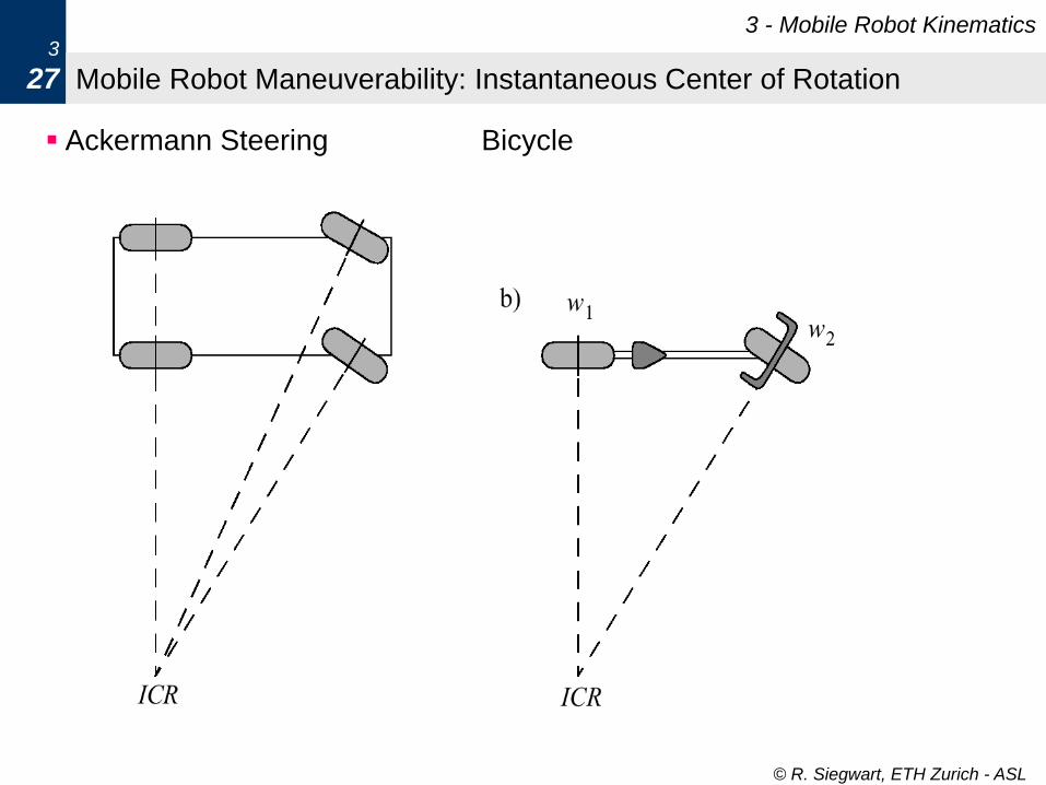
27 Mobile Robot Maneuverability: Instantaneous Center of Rotation

Ackermann Steering Bicycle

APPLICATION: WHEEL CONTROL


28

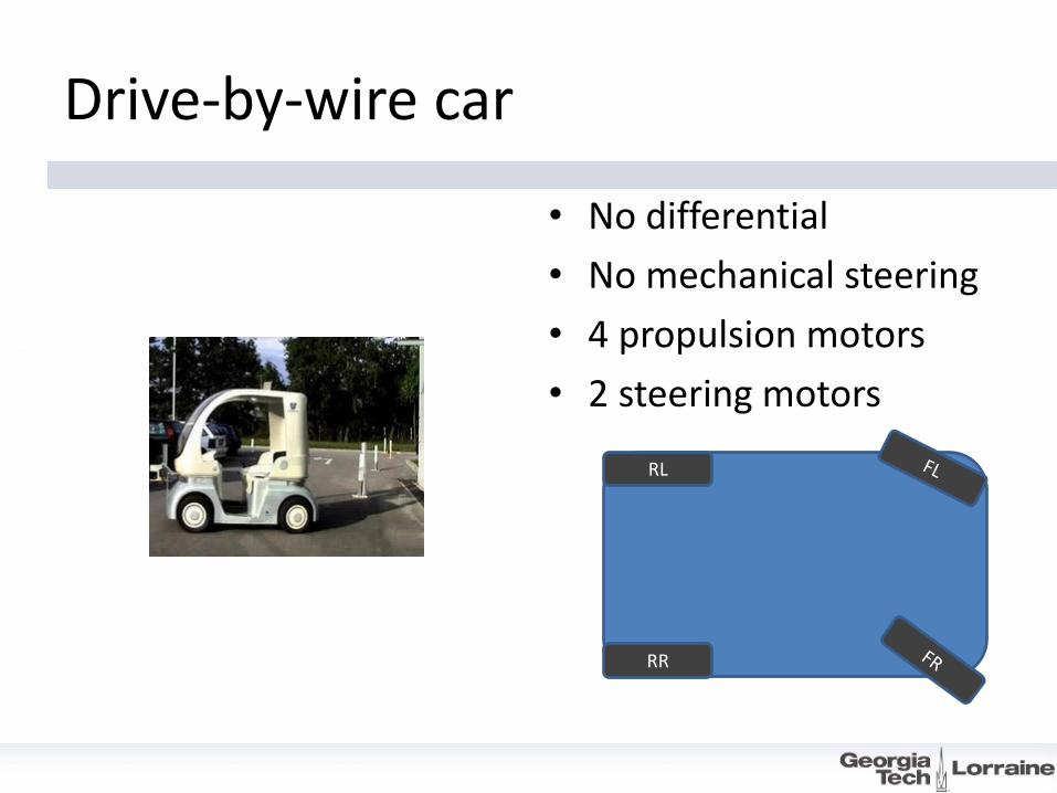
Drive-by-wire car

• No differential

• No mechanical steering

• 4 propulsion motors

• 2 steering motors

RL

RR

Wheel control

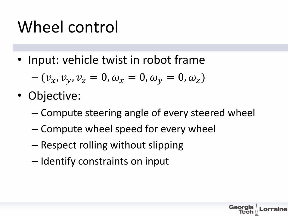
• Input: vehicle twist in robot frame

– (𝑣𝑥, 𝑣𝑦, 𝑣𝑧 = 0,𝜔𝑥 = 0,𝜔𝑦 = 0,𝜔𝑧)

• Objective:

– Compute steering angle of every steered wheel

– Compute wheel speed for every wheel

– Respect rolling without slipping

– Identify constraints on input

Wheel control

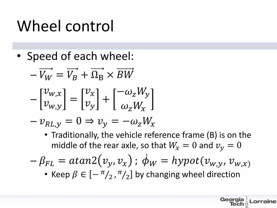
• Speed of each wheel:

– 𝑉𝑊 = 𝑉𝐵 + ΩB × 𝐵𝑊

–𝑣𝑤,𝑥𝑣𝑤,𝑦

=𝑣𝑥𝑣𝑦

+−𝜔𝑧𝑊𝑦

𝜔𝑧𝑊𝑥

– 𝑣𝑅𝐿,𝑦 = 0 ⇒ 𝑣𝑦 = −𝜔𝑧𝑊𝑥 • Traditionally, the vehicle reference frame (B) is on the

middle of the rear axle, so that 𝑊𝑥 = 0 and 𝑣𝑦 = 0

– 𝛽𝐹𝐿 = 𝑎𝑡𝑎𝑛2 𝑣𝑦, 𝑣𝑥 ; 𝜙 𝑊 = ℎ𝑦𝑝𝑜𝑡(𝑣𝑤,𝑦, 𝑣𝑤,𝑥) • Keep 𝛽 ∈ − 𝜋

2 , 𝜋 2 by changing wheel direction

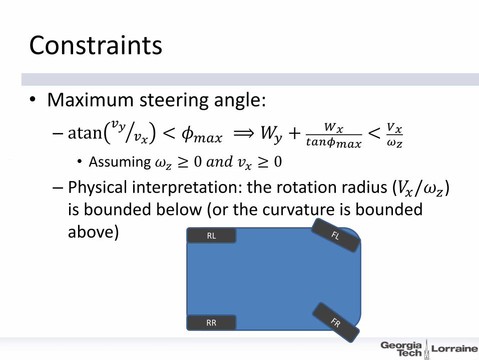
Constraints

• Maximum steering angle:

– atan𝑣𝑦

𝑣𝑥 < 𝜙𝑚𝑎𝑥 ⟹ 𝑊𝑦 +𝑊𝑥

𝑡𝑎𝑛𝜙𝑚𝑎𝑥< 𝑉𝑥

𝜔𝑧

• Assuming 𝜔𝑧 ≥ 0 𝑎𝑛𝑑 𝑣𝑥 ≥ 0

– Physical interpretation: the rotation radius (𝑉𝑥/𝜔𝑧) is bounded below (or the curvature is bounded above)

RL

RR

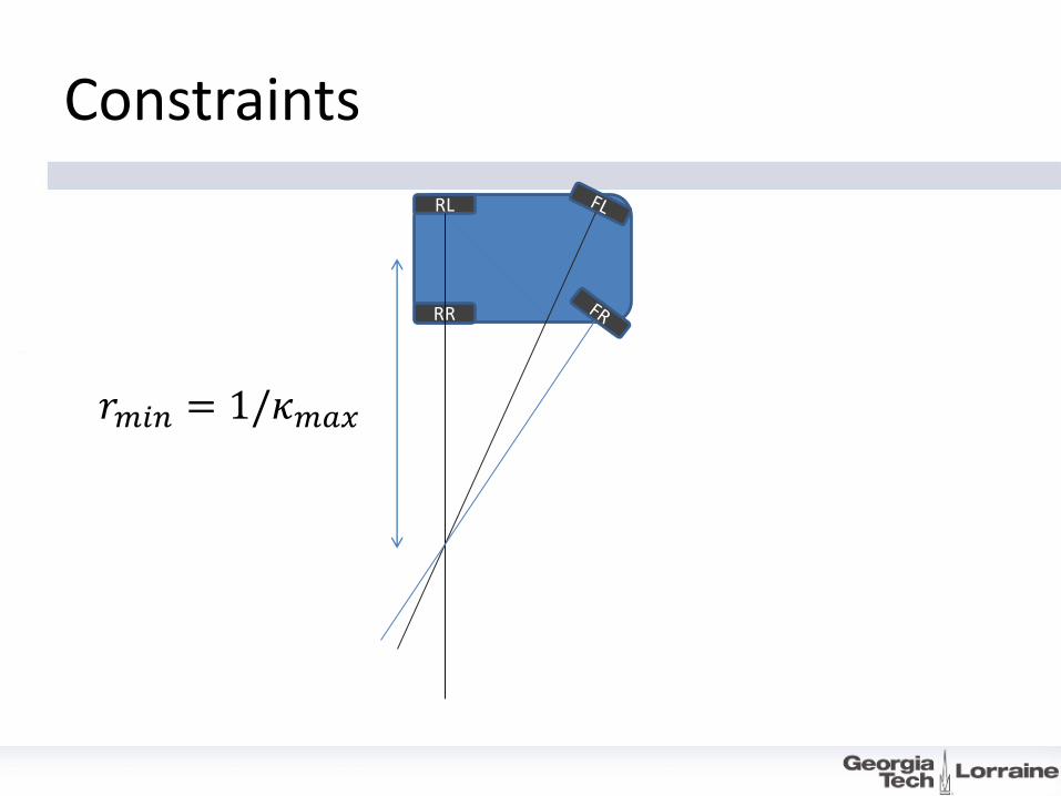
Constraints

RL

RR

𝑟𝑚𝑖𝑛 = 1/𝜅𝑚𝑎𝑥

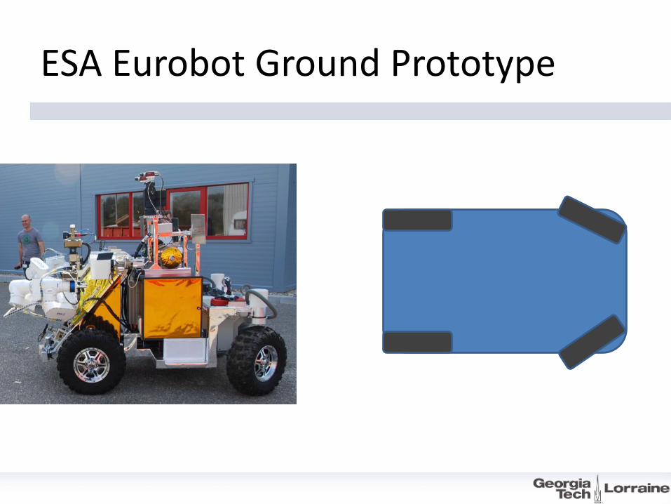
ESA Eurobot Ground Prototype

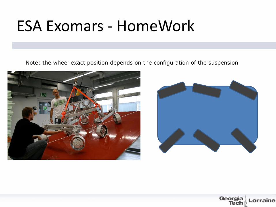
ESA Exomars - HomeWork

Note: the wheel exact position depends on the configuration of the suspension

APPLICATION: WHEEL ODOMETRY


36

Drive-by-wire car

• No differential

• No mechanical steering

• 4 propulsion motors

• 2 steering motors

RL

RR

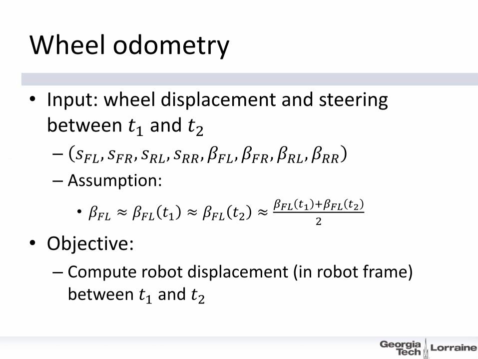
Wheel odometry

• Input: wheel displacement and steering between 𝑡1 and 𝑡2

– 𝑠𝐹𝐿, 𝑠𝐹𝑅, 𝑠𝑅𝐿, 𝑠𝑅𝑅, 𝛽𝐹𝐿, 𝛽𝐹𝑅 , 𝛽𝑅𝐿, 𝛽𝑅𝑅

– Assumption:

• 𝛽𝐹𝐿 ≈ 𝛽𝐹𝐿 𝑡1 ≈ 𝛽𝐹𝐿 𝑡2 ≈𝛽𝐹𝐿 𝑡1 +𝛽𝐹𝐿 𝑡2

2

• Objective:

– Compute robot displacement (in robot frame) between 𝑡1 and 𝑡2

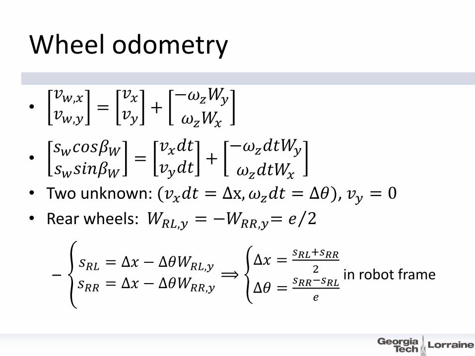
Wheel odometry

•𝑣𝑤,𝑥𝑣𝑤,𝑦

=𝑣𝑥𝑣𝑦

+−𝜔𝑧𝑊𝑦

𝜔𝑧𝑊𝑥

•𝑠𝑤𝑐𝑜𝑠𝛽𝑊𝑠𝑤𝑠𝑖𝑛𝛽𝑊

=𝑣𝑥𝑑𝑡𝑣𝑦𝑑𝑡

+−𝜔𝑧𝑑𝑡𝑊𝑦

𝜔𝑧𝑑𝑡𝑊𝑥

• Two unknown: (𝑣𝑥𝑑𝑡 = Δx,𝜔𝑧𝑑𝑡 = Δ𝜃), 𝑣𝑦 = 0

• Rear wheels: 𝑊𝑅𝐿,𝑦 = −𝑊𝑅𝑅,𝑦= 𝑒 2

– 𝑠𝑅𝐿 = Δ𝑥 − Δ𝜃𝑊𝑅𝐿,𝑦

𝑠𝑅𝑅 = Δ𝑥 − Δ𝜃𝑊𝑅𝑅,𝑦⟹

Δ𝑥 =𝑠𝑅𝐿+𝑠𝑅𝑅

2

Δ𝜃 =𝑠𝑅𝑅−𝑠𝑅𝐿

𝑒

in robot frame

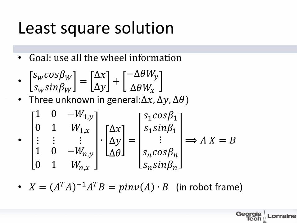
Least square solution

• Goal: use all the wheel information

•𝑠𝑤𝑐𝑜𝑠𝛽𝑊𝑠𝑤𝑠𝑖𝑛𝛽𝑊

=Δ𝑥Δ𝑦

+−Δ𝜃𝑊𝑦

Δ𝜃𝑊𝑥

• Three unknown in general:Δ𝑥, Δ𝑦, Δ𝜃)

•

1 0 −𝑊1,𝑦

0 1 𝑊1,𝑥

⋮ ⋮ ⋮1 0 −𝑊𝑛,𝑦

0 1 𝑊𝑛,𝑥

∙Δ𝑥Δ𝑦Δ𝜃

=

𝑠1𝑐𝑜𝑠𝛽1𝑠1𝑠𝑖𝑛𝛽1

⋮𝑠𝑛𝑐𝑜𝑠𝛽𝑛𝑠𝑛𝑠𝑖𝑛𝛽𝑛

⟹ 𝐴 𝑋 = 𝐵

• 𝑋 = 𝐴𝑇𝐴 −1𝐴𝑇𝐵 = 𝑝𝑖𝑛𝑣 𝐴 ∙ 𝐵 (in robot frame)

ESA Exomars - HomeWork

Note: the wheel exact position depends on the configuration of the suspension

MOBILITY QUANTIFICATION



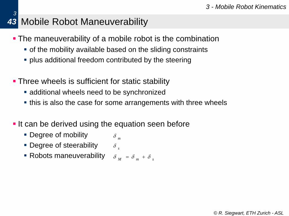
43 Mobile Robot Maneuverability

The maneuverability of a mobile robot is the combination

of the mobility available based on the sliding constraints

plus additional freedom contributed by the steering

Three wheels is sufficient for static stability

additional wheels need to be synchronized

this is also the case for some arrangements with three wheels

It can be derived using the equation seen before

Degree of mobility

Degree of steerability

Robots maneuverability

m

s

smM



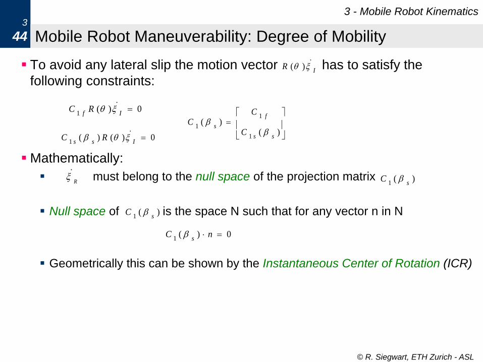
44 Mobile Robot Maneuverability: Degree of Mobility

To avoid any lateral slip the motion vector has to satisfy the

following constraints:

Mathematically:

must belong to the null space of the projection matrix

Null space of is the space N such that for any vector n in N

Geometrically this can be shown by the Instantaneous Center of Rotation (ICR)

0)(1

If

RC

)()(

1

1

1

ss

f

sC

CC

0)()(1

Iss

RC

IR )(

R )(

1 sC

)(1 s

C

0)(1

nCs



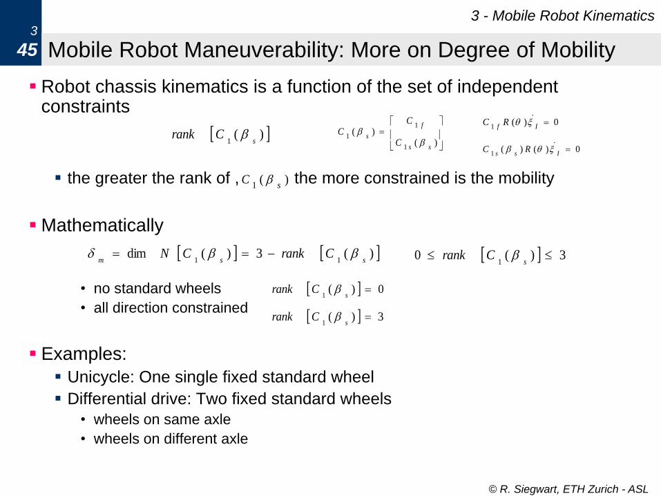
45 Mobile Robot Maneuverability: More on Degree of Mobility

Robot chassis kinematics is a function of the set of independent constraints

the greater the rank of , the more constrained is the mobility

Mathematically

• no standard wheels

• all direction constrained

Examples:

Unicycle: One single fixed standard wheel

Differential drive: Two fixed standard wheels

• wheels on same axle

• wheels on different axle

)( 1 s

Crank

)(1 s

C

)( 3)( dim11 ssm

CrankCN 3)( 01

s

Crank

0)( 1

s

Crank

3)( 1

s

Crank

0)(1

If

RC

)()(

1

1

1

ss

f

sC

CC

0)()(1

Iss

RC



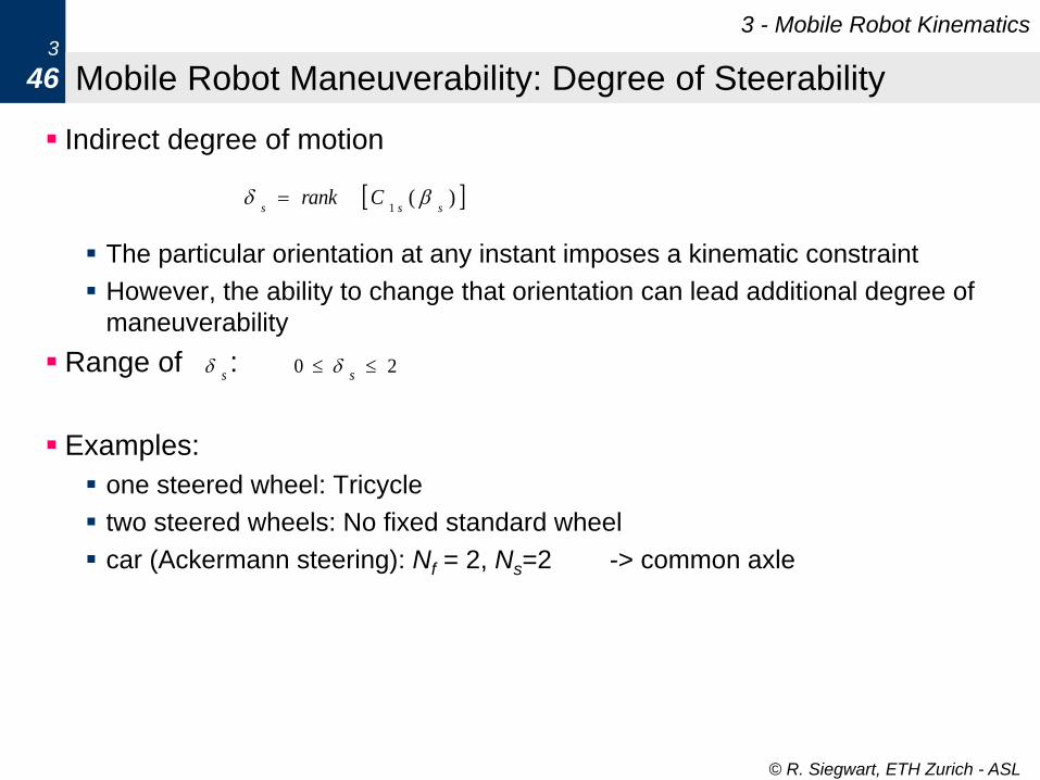
46 Mobile Robot Maneuverability: Degree of Steerability

Indirect degree of motion

The particular orientation at any instant imposes a kinematic constraint

However, the ability to change that orientation can lead additional degree of

maneuverability

Range of :

Examples:

one steered wheel: Tricycle

two steered wheels: No fixed standard wheel

car (Ackermann steering): Nf = 2, Ns=2 -> common axle

)( 1 sss

Crank

20 s

s



47 Mobile Robot Maneuverability: Robot Maneuverability

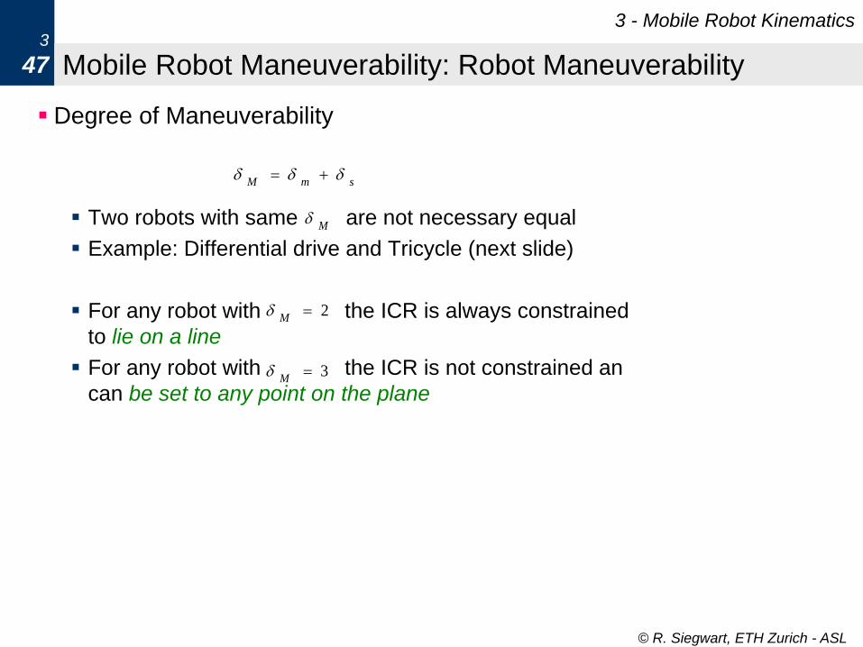
Degree of Maneuverability

Two robots with same are not necessary equal

Example: Differential drive and Tricycle (next slide)

For any robot with the ICR is always constrained

to lie on a line

For any robot with the ICR is not constrained an

can be set to any point on the plane

smM

M

3M

2M



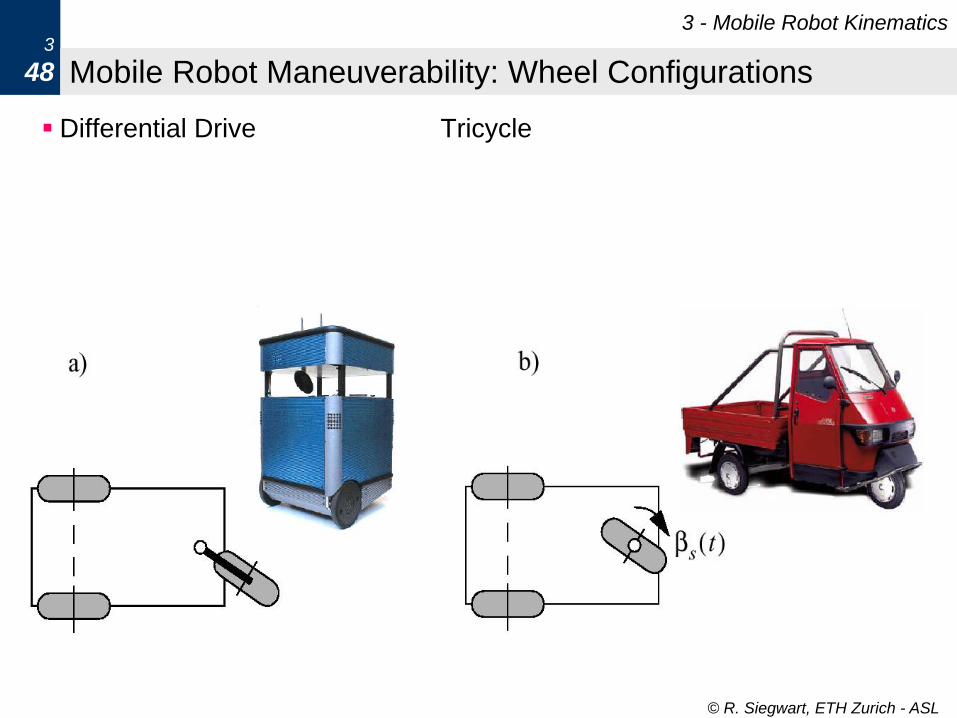
48 Mobile Robot Maneuverability: Wheel Configurations

Differential Drive Tricycle



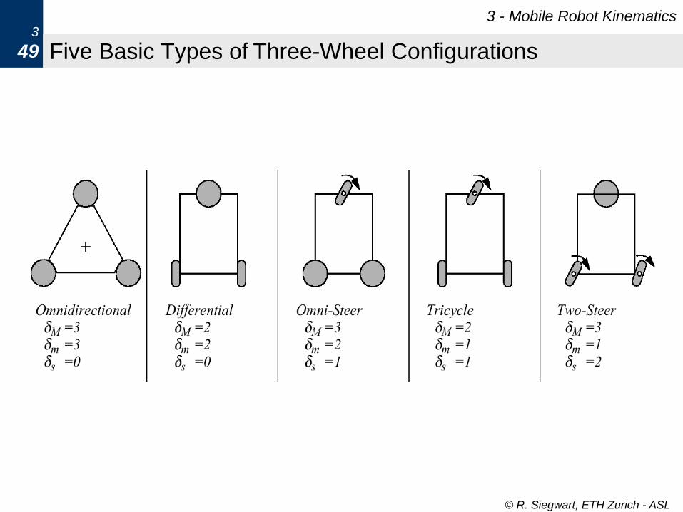
49 Five Basic Types of Three-Wheel Configurations



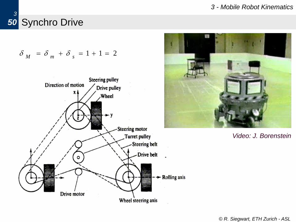
50 Synchro Drive

211 smM

Video: J. Borenstein



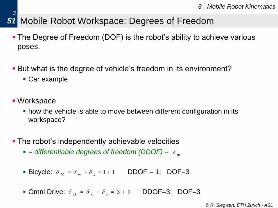
51 Mobile Robot Workspace: Degrees of Freedom

The Degree of Freedom (DOF) is the robot’s ability to achieve various

poses.

But what is the degree of vehicle’s freedom in its environment?

Car example

Workspace

how the vehicle is able to move between different configuration in its

workspace?

The robot’s independently achievable velocities

= differentiable degrees of freedom (DDOF) =

Bicycle: DDOF = 1; DOF=3

Omni Drive: DDOF=3; DOF=3

m

11 smM

03 smM



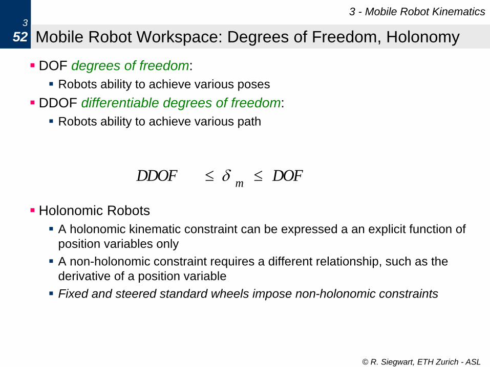
52 Mobile Robot Workspace: Degrees of Freedom, Holonomy

DOF degrees of freedom:

Robots ability to achieve various poses

DDOF differentiable degrees of freedom:

Robots ability to achieve various path

Holonomic Robots

A holonomic kinematic constraint can be expressed a an explicit function of

position variables only

A non-holonomic constraint requires a different relationship, such as the

derivative of a position variable

Fixed and steered standard wheels impose non-holonomic constraints

DOFDDOFm


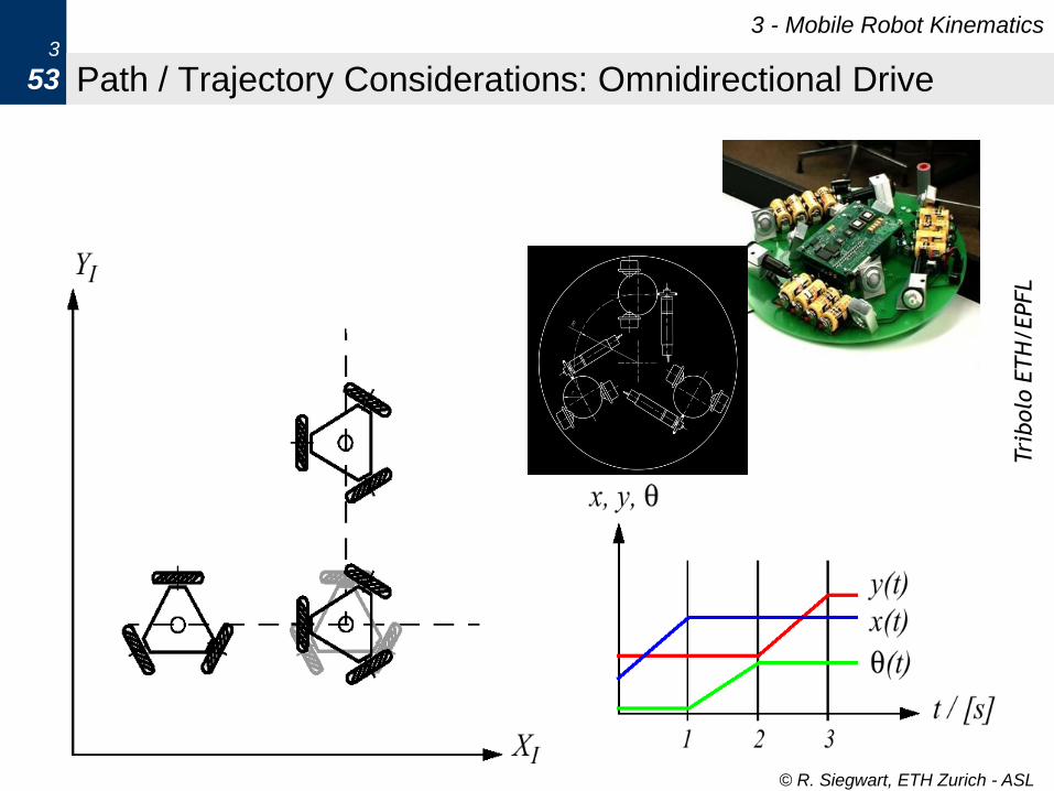
Path / Trajectory Considerations: Omnidirectional Drive


53

Tri

bolo

ETH

/EPFL


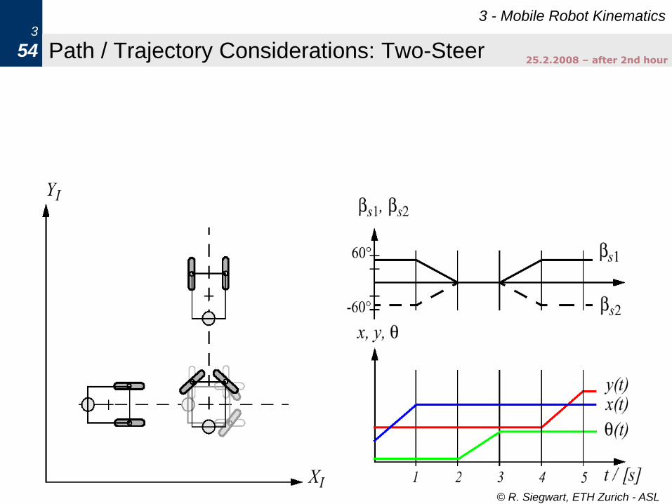
Path / Trajectory Considerations: Two-Steer


54 25.2.2008 – after 2nd hour

NON-HOLONOMIC ROBOTS



56 Mobile Robot Kinematics: Non-Holonomic Systems

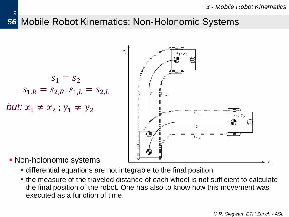
Non-holonomic systems

differential equations are not integrable to the final position.

the measure of the traveled distance of each wheel is not sufficient to calculate the final position of the robot. One has also to know how this movement was executed as a function of time.

s1 L

s1 R

s2 L

s2 R

yI

xI

x1

, y1

x2

, y2

s1

s2

𝑠1 = 𝑠2 𝑠1,𝑅 = 𝑠2,𝑅; 𝑠1,𝐿 = 𝑠2,𝐿

but: 𝑥1 ≠ 𝑥2 ; 𝑦1 ≠ 𝑦2



57 Non-Holonomic Systems: Mathematical Interpretation

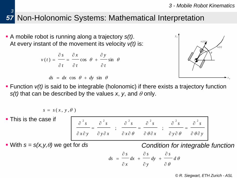
A mobile robot is running along a trajectory s(t).

At every instant of the movement its velocity v(t) is:

Function v(t) is said to be integrable (holonomic) if there exists a trajectory function

s(t) that can be described by the values x, y, and only.

This is the case if

With s = s(x,y,) we get for ds

yI

xI

s ( t)

v ( t)

sincos)(

t

y

t

x

t

stv

sincos dydxds

),,( yxss

y

s

y

s

x

s

x

s

xy

s

yx

s

222222

; ;

ds

dy

y

sdx

x

sds

Condition for integrable function

Lie brackets

• Differential tool to analyze the mobility of a system (many other uses outside of robotics)

• Informally:

– An infinitely small parallel-parking maneuver is a way to move out of the local manifold spanned by the kinematic constraints.

• Lecture from Matt Mason (CMU): – http://www.cs.cmu.edu/afs/cs/academic/class/16741-

s07/www/lecture5.pdf




ARTICLES

Articles

• A novel approach for steering wheel synchronization with velocity/acceleration limits and mechanical constraints, U. Schwesinger, C. Pradalier, R. Siegwart, IROS’12

• Terrain Mapping and Control Optimization for a 6-Wheel Rover with Passive Suspension, P. Strupler , C. Pradalier, R. Siegwart, FSR’12

• Modeling odometry and uncertainty propagation for a Bi-Steerable car, J. Hermosillo, C. Pradalier, S. Sekhavat, IV’02

• 3D-Odometry for rough terrain – Towards real 3D navigation, P. Lamon and R. Siegwart, ICRA’03

• 3D Localization for the MagneBike Inspection Robot, F. Tache, F. Pomerleau, G. Caprari, R. Siegwart, R. Moser, M. Bosse, JFR 2011

• Simultaneous Localization and Odometry Calibration for Mobile Robot, A. Martinelli, N. Tomatis, A. Tapus and R. Siegwart, IROS’03

http://ieeexplore.ieee.org/xpls/abs_all.jsp?arnumber=6385644




http://publications.asl.ethz.ch/files/strupler12terrain.pdf







http://infoscience.epfl.ch/record/97505/files/Odometry3DIcra2003_.pdf







http://publications.asl.ethz.ch/files/tache11three.pdf





http://www.ensta-paristech.fr/~tapus/publications_files/tapus_IROS2003a.pdf



CONCLUSION

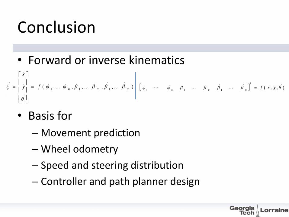
Conclusion

• Forward or inverse kinematics

• Basis for

– Movement prediction

– Wheel odometry

– Speed and steering distribution

– Controller and path planner design

),,,,, (111 mmn

fy

x

),, ( 111

yxfT

mmn

7630 Autonomous Robotics Mobile Robot Kinematicsdream.georgiatech-metz.fr/sites/default/files/3 -...

Documents

Transcript of 7630 Autonomous Robotics Mobile Robot Kinematicsdream.georgiatech-metz.fr/sites/default/files/3 -...