DESIGN AND ANALYSIS OF HONEYCOMB STRUCTURES WITH

ADVANCED CELL WALLS

A Dissertation

by

RUOSHUI WANG

Submitted to the Office of Graduate and Professional Studies of

Texas A&M University

in partial fulfillment of the requirements for the degree of

DOCTOR OF PHILOSOPHY

Chair of Committee, Xinghang Zhang

Co-Chair of Committee, Jyhwen Wang

Committee Members, Amine Benzerga

Karl 'Ted' Hartwig

Head of Department, Ibrahim Karaman

December 2016

Major Subject: Materials Science and Engineering

Copyright 2016 Ruoshui Wang

ii

ABSTRACT

Honeycomb structures are widely used in engineering applications. This work

consists of three parts, in which three modified honeycombs are designed and analyzed.

The objectives are to obtain honeycomb structures with improved specific stiffness and

specific buckling resistance while considering the manufacturing feasibility.

The objective of the first part is to develop analytical models for general case

honeycombs with non-linear cell walls. Using spline curve functions, the model can

describe a wide range of 2-D periodic structures with nonlinear cell walls. The derived

analytical model is verified by comparing model predictions with other existing models,

finite element analysis (FEA) and experimental results. Parametric studies are conducted

by analytical calculation and finite element modeling to investigate the influences of the

spline waviness on the homogenized properties. It is found that, comparing to straight cell

walls, spline cell walls have increased out-of-plane buckling resistance per unit weight,

and the extent of such improvement depends on the distribution of the spline’s curvature.

The second part of this research proposes a honeycomb with laminated composite

cell walls, which offer a wide selection of constituent materials and improved specific

stiffness. Analytical homogenization is established and verified by FEA comparing the

mechanical responses of a full-detailed honeycomb and a solid cuboid assigned with the

calculated homogenization properties. The results show that the analytical model is

accurate at a small computational cost. Parametric studies reveal nonlinear relationships

iii

between the ply thickness and the effective properties, based on which suggestions are

made for property optimizations.

The third part studies honeycomb structures with perforated cell walls. The

homogenized properties of this new honeycomb are analytically modeled and investigated

by finite element modeling. It is found that comparing to conventional honeycombs,

honeycombs with perforated cell walls demonstrate enhanced in-plane stiffness, out-of-

plane bending rigidity, out-of-plane compressive buckling stress, approximately the same

out-of-plane shear buckling strength, and reduced out-of-plane stiffness. For the future

design, empirical formulas, based on finite element results and expressed as functions of

the perforation size, are derived for the mechanical properties and verified by mechanical

tests conducted on a series of 3D printed perforated honeycomb specimens.

iv

ACKNOWLEDGEMENTS

I would like to thank my committee chair and co-chair, Dr. Zhang and Dr. Wang,

and my committee members, Dr. Benzerga, and Dr. Hartwig, for their guidance and

support throughout the course of this research.

I would also like to thank my colleagues, Cheng-Kang Yang and Ying Zhang, for

providing me assists and advice on my research. Thanks also go to my friends and the

department faculty and staff for making my time at Texas A&M University a great

experience.

Finally, I’d like to thank my mother Xiaoli Yang and father Xiaojun Wang for their

encouragement and to my wife, Feng Jiang, for her patience and love during the last year

of my study.

v

TABLE OF CONTENTS

Page

ABSTRACT .......................................................................................................................ii

ACKNOWLEDGEMENTS .............................................................................................. iv

TABLE OF CONTENTS ................................................................................................... v

LIST OF FIGURES ..........................................................................................................vii

LIST OF TABLES ............................................................................................................ xi

1. INTRODUCTION ......................................................................................................... 1

1.1 Literature Review on Honeycomb Materials ....................................................... 2

1.2 Honeycombs with Spline Cell Walls .................................................................. 10

1.3 Honeycombs with Composite Laminated Cell Walls ........................................ 12

1.4 Honeycombs with Perforated Cell Walls ........................................................... 13

1.5 Research Objectives ........................................................................................... 16

2. HONEYCOMBS WITH SPLINE CELL WALLS.......................................................19

2.1 Analytical Modeling ........................................................................................... 19

2.1.1 Bezier Curve Function ................................................................................ 19

2.1.2 In-plane Properties ...................................................................................... 21

2.1.3 Out-of-plane Properties ............................................................................... 24

2.1.4 Boundary Condition: Horizontal Plates ...................................................... 25

2.1.5 Boundary Condition: Bonding Strips .......................................................... 27

2.2 Verification ......................................................................................................... 29

2.2.1 Analytical Verification ................................................................................ 29

2.2.2 Experimental Verification ........................................................................... 32

2.3 Parametric Study and Discussions ..................................................................... 36

2.3.1 FEA Models ................................................................................................ 36

2.3.2 In-plane Stiffness ........................................................................................ 38

2.3.3 Out-of-plane Stability.................................................................................. 39

2.4 Conclusions ........................................................................................................ 42

3. HONEYCOMBS WITH LAMINATED COMPOSITE CELL WALLS .................... 44

3.1 Analytical Modeling ........................................................................................... 44

3.1.1 In-plane Elastic Moduli ............................................................................... 44

vi

Page

3.1.2 In-plane Shear Modulus .............................................................................. 47

3.1.3 Out-of-plane Elastic Modulus ..................................................................... 47

3.1.4 Out-of-plane Shear Moduli ......................................................................... 48

3.1.5 Poisson’s Ratios .......................................................................................... 49

3.2 Numerical Modeling ........................................................................................... 49

3.3 Result and Discussion ........................................................................................ 52

3.3.1 In-plane Mechanical Behaviors ................................................................... 52

3.3.2 Out-of-plane Mechanical Behaviors ........................................................... 56

3.4 Conclusions ........................................................................................................ 59

4. HONEYCOMBS WITH PERFORATED CELL WALLS .......................................... 61

4.1 Analytical Modeling ........................................................................................... 61

4.1.1 Theoretical Considerations.......................................................................... 61

4.1.2 In-plane Moduli ...........................................................................................62

4.1.3 Out-of-plane Compressive Critical Buckling Stress ...................................70

4.2 Finite Element Modeling and Empirical Formulas ............................................ 73

4.2.1 Methodologies .............................................................................................74

4.2.2 In-plane Elastic Moduli ...............................................................................79

4.2.3 In-plane Shear Modulus .............................................................................. 81

4.2.4 Out-of-plane Elastic Modulus ..................................................................... 83

4.2.5 Out-of-plane Shear Moduli ......................................................................... 85

4.2.6 Out-of-plane Bending Rigidity ................................................................... 88

4.2.7 Out-of-plane Critical Compressive Stress ................................................... 91

4.2.8 Out-of-plane Critical Shear Stress .............................................................. 94

4.3 Experimental Verification .................................................................................. 98

4.4 Results and Discussion ..................................................................................... 100

4.5 Conclusions ...................................................................................................... 105

5. SUMMARY AND FUTURE WORK........................................................................ 108

REFERENCES............................................................................................................... 110

vii

LIST OF FIGURES

Page

Fig. 1.1. Two widely used honeycomb manufacturing processes. (a) Bonding-

expanding process; (b) Corrugation-welding process [10]. ................................ 2

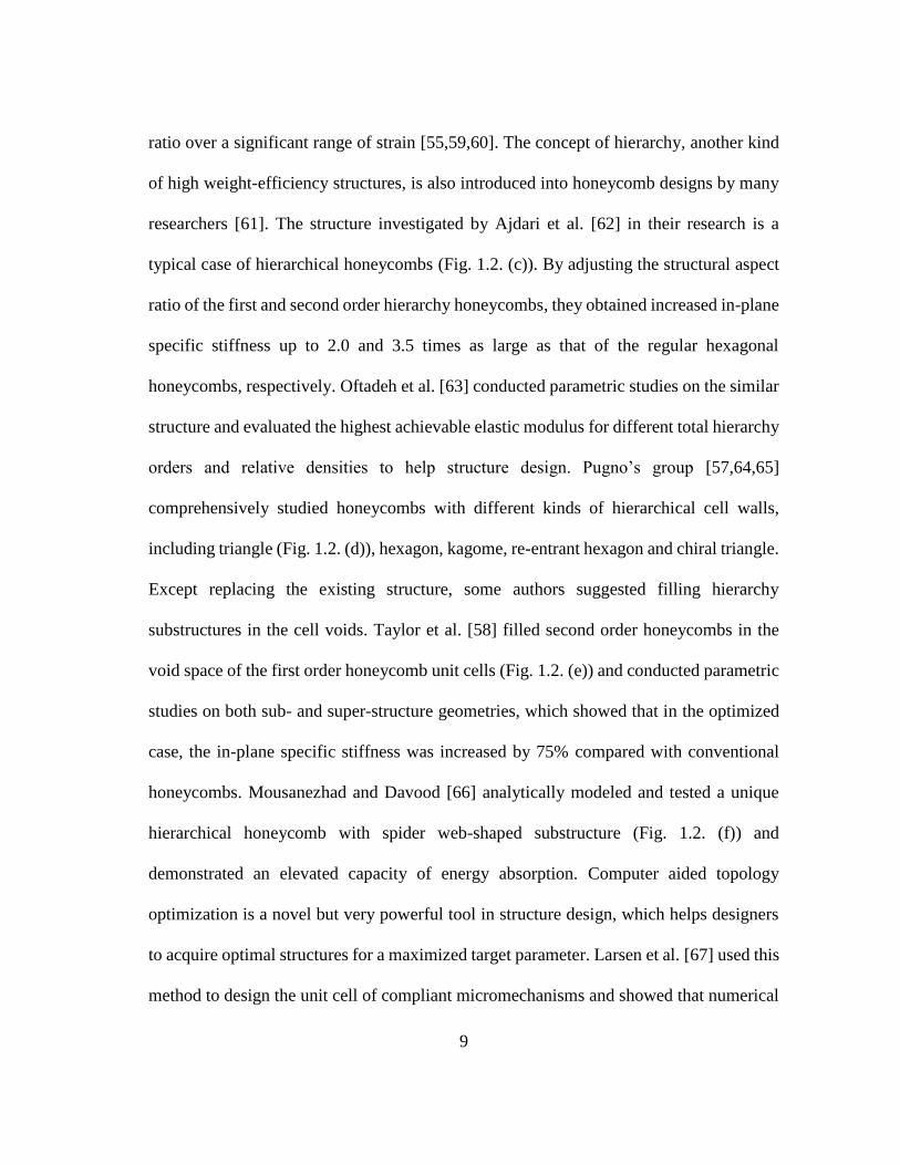
Fig. 1.2. Examples of honeycombs with substructures. (a) Cylinder joint honeycomb

[54]; (b) auxetic chiral honeycomb [55]; (c) honeycomb with hierarchy

joints [56]; (d) honeycomb with hierarchy cell walls [57]; (e) multi-order

honeycomb [58]; (f) spider web hone ................................................................. 8

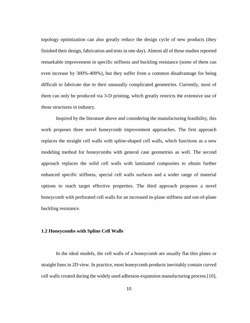
Fig. 1.3. Honeycomb with nonlinear cell walls. (a) Curvature formed during

bonding-expanding process; (b) Wavy cell walls to increase buckling

resistance. .......................................................................................................... 12

Fig. 2.1. Unit cell of honeycombs with spline cell walls. ............................................... 21

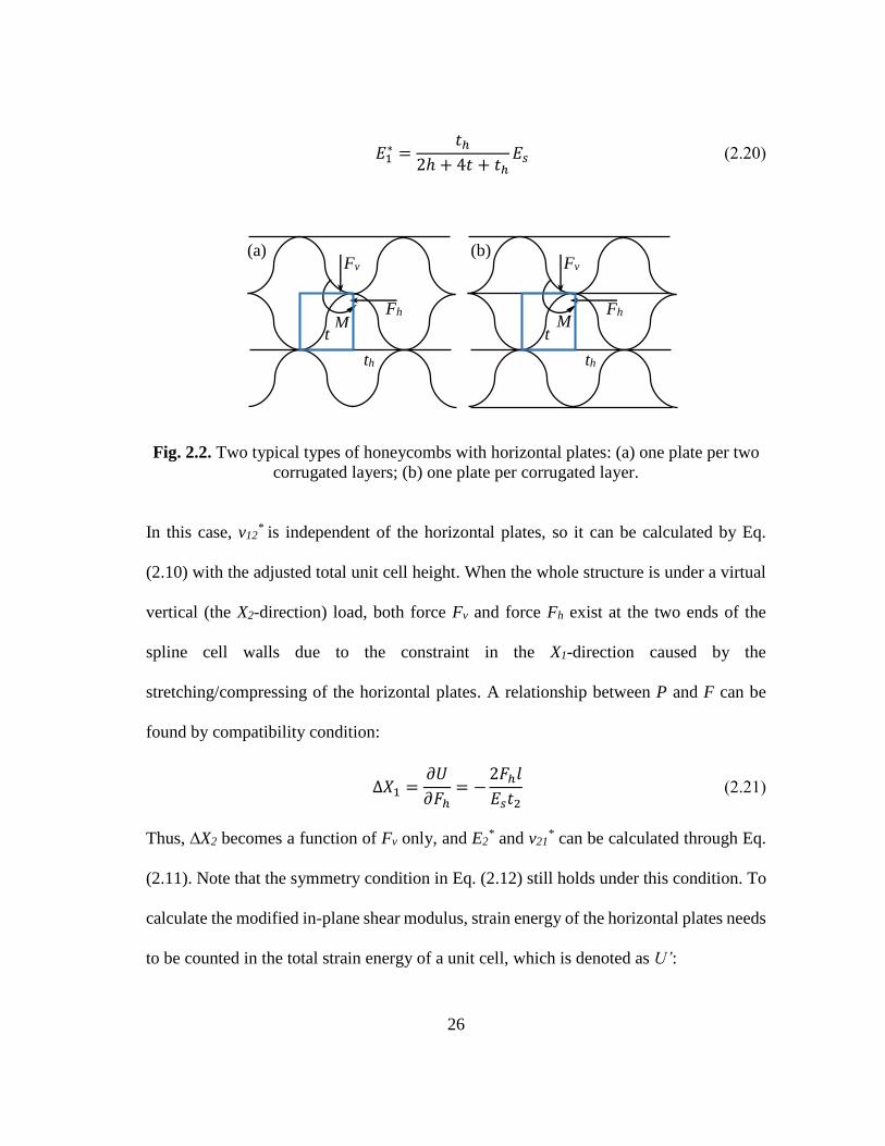
Fig. 2.2. Two typical types of honeycombs with horizontal plates: (a) one plate per

two corrugated layers; (b) one plate per corrugated layer. ............................... 26

Fig. 2.3. (a) Honeycomb with bonding strips instead of bonding lines and (b) its unit

cell. .................................................................................................................... 29

Fig. 2.4. Effective in-plane elastic and shear moduli of hexagonal honeycombs that

are calculated by Gibson and Ashby’s model and the Spline curve model. ..... 31

Fig. 2.5. Effective in-plane transverse elastic and shear moduli of sinusoidal

honeycombs that are calculated by Qiao and Wang’s model and the Spline

curve model. ..................................................................................................... 31

Fig. 2.6. Es/E2* versus unit cell length l. ......................................................................... 32

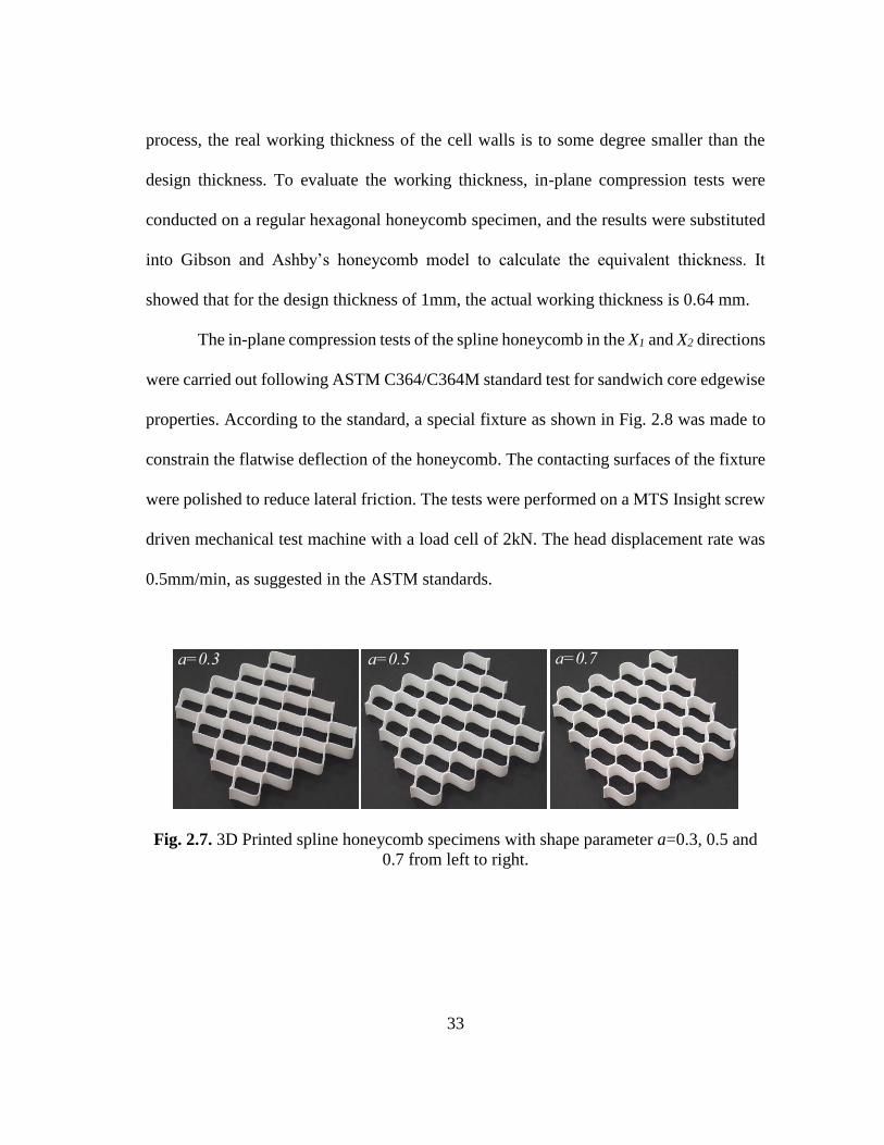
Fig. 2.7. 3D Printed spline honeycomb specimens with shape parameter a=0.3, 0.5

and 0.7 from left to right. .................................................................................. 33

Fig. 2.8. Fixture set for edgewise compression test of honeycomb sandwich cores. ...... 34

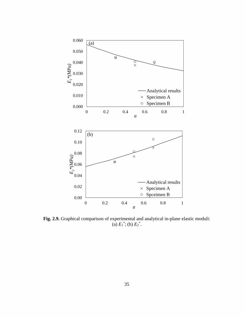
Fig. 2.9. Graphical comparison of experimental and analytical in-plane elastic

moduli: (a) E1*; (b) E2

*. .................................................................................... 35

Fig. 2.10. Finite element unit cell selected from a honeycomb with spline cell walls. ..... 37

viii

Page

Fig. 2.11. The three unit cell aspect ratios with varying spline shape parameters built

in the finite element models. ............................................................................. 37

Fig. 2.12. Normalized effective in-plane moduli versus spline shape parameter under

the three unit cell aspect ratios .......................................................................... 39

Fig. 2.13. Specific out-of-plane buckling stress versus spline shape parameter under

the three unit cell aspect. .................................................................................. 41

Fig. 2.14. First buckling modes of spline cell walls with selected shape parameters

under three aspect ratios. .................................................................................. 42

Fig. 3.1. The bending mode of the inclined cell walls when the honeycomb is

subjected to uniform in-plane compression. ..................................................... 45

Fig. 3.2. Cross section of an n-layer laminated composite honeycomb cell wall. .......... 47

Fig. 3.3. (a) Honeycomb with double-layer cell walls. (b) Ply arrangement in

junction area. ..................................................................................................... 50

Fig. 3.4. FE models built for verification and parametric study. (a) Full detailed

honeycomb model with composite shell elements; (b) cuboid model with

calculated effective properties. ......................................................................... 51

Fig. 3.5. (a) F1n-t1 response of X1 uniaxial compression. (b) Stress contour of the

deformed full detailed model ............................................................................ 53

Fig. 3.6. (a) F2n-t2 response of X2 uniaxial compression. (b) Stress contour of the

deformed full detailed model ............................................................................ 54

Fig. 3.7. (a) F12n-t1 response of X1-X2 shear. (b) Stress contour of the deformed full

detailed model (c) Stress contour of the deformed homogenized model ......... 55

Fig. 3.8. (a) F3n-t1 response of X3 compression. (b) Stress contour of the deformed

homogenized model .......................................................................................... 57

Fig. 3.9. (a) F13n-t1 response of X1-X3 shear. (b) Stress contour of the deformed full

detailed model ................................................................................................... 57

Fig. 3.10. (a) F23n-t1 response of X2-X3 shear. (b) Stress contour of the deformed full

detailed model. .................................................................................................. 58

ix

Page

Fig. 4.1. (a) Bending mode of the honeycomb cell walls under uniform external in-

plane load and (b) its equivalent form of two cantilever beams. ...................... 62

Fig. 4.2. A half perforated cell wall subjected to cantilever-type bending. .................... 63

Fig. 4.3. Eight equally spaced points selected on the x=l/2 and y=l/2 edges. ................ 67

Fig. 4.4. Deflection surface of a perforated cell wall with 2R/l=0.75. ............................ 68

Fig. 4.5. Approximated equivalent shape of a perforated cell wall under bending, the

crosshatch regions have the same area. ............................................................ 69

Fig. 4.6. Representative volume element (RVE) model used in finite element testes

in (a) 2D view and (b) 3D view. ....................................................................... 75

Fig. 4.7. Mesh density convergence of S4 and S8R element under three types of

loads .................................................................................................................. 76

Fig. 4.8. Stress contour of the deformed inclined cell wall of a honeycomb under

uniform in-plane compression. ......................................................................... 79

Fig. 4.9. In-plane elastic moduli of perforated honeycombs vs. 2R/l. ............................ 80

Fig. 4.10. Stress contour of the deformed RVE under in-plane shear ............................... 82

Fig. 4.11. In-plane shear modulus of perforated honeycombs vs. 2R/l ............................. 82

Fig. 4.12. Deformation of the RVE under out-of-plane compression ............................... 84

Fig. 4.13. Out-of-plane elastic modulus of perforated honeycombs vs. 2R/l .................... 84

Fig. 4.14. Deformation of the RVE under out-of-plane shear in the (a) X1-X3 direction

and (b) X2-X3 direction ...................................................................................... 86

Fig. 4.15. Out-of-plane shear moduli of perforated honeycombs vs. 2R/l ........................ 86

Fig. 4.16. Deflection of an inclined cell wall under overall uniform out-of-plane

bending ............................................................................................................. 89

Fig. 4.17. Out-of-plane bending rigidities of perforated honeycombs vs. 2R/l ................. 89

Fig. 4.18. First buckling mode of the RVE under out-of-plane compression with (a)

simply supported connection and (b) clamped connection. .............................. 92

x

Page

Fig. 4.19. Out-of-plane compressive buckling stress of perforated honeycombs vs.

2R/l. ................................................................................................................... 92

Fig. 4.20. First buckling mode of the RVE under out-of-plane shear loads. (a) X1-X3

shear with simply supported connection; (b) X2-X3 shear with simply

supported connection; (c) X1-X3 shear with clamped connection; (d) X2-X3

shear with clamped connection. ........................................................................ 95

Fig. 4.21. Out-of-plane critical shear stress of perforated honeycombs vs. 2R/l in the

(a) X1-X3 and (b)X2-X3 directions ...................................................................... 96

Fig. 4.22. 3D Printed perforated honeycomb specimens with 2R/l=0.25, 2R/l=0.5 and

2R/l=0.75, from left to right. ........................................................................... 100

Fig. 4.23. Experiment setups for (a) in-plane (edgewise) compression tests and (b) out-

of-plane compression tests. ............................................................................. 100

Fig. 4.24. Graphical comparison of analytical, empirical and experimental results of

in-plane elastic moduli. ................................................................................... 102

Fig. 4.25. Graphical comparison of analytical, empirical and experimental results of

the homogenized out-of-plane critical stress. ................................................. 104

Fig. 4.26. The buckling modes of the deformed specimens and the RVE with (a)

2R/l=0.25, (b) 2R/l=0.5, (c) 2R/l=0.75 ........................................................... 105

xi

LIST OF TABLES

Page

Table 4.1. Modeling details of the finite element honeycomb RVE ................................ 76

Table 4.2. Geometric parameters and material properties of the finite element RVE ..... 77

Table 4.3. Properties change brought by the perforations at three 2R/l ratios ............... 107

1

1. INTRODUCTION

Honeycombs are 2-D cellular materials with a regular periodic microstructure

inspired from biological structures such as bee hives, microstructure of abalone shells and

bamboo cross-sections [1–3]. As one of the most famous product of bionic engineering

in human history, honeycombs provide ideal solutions for the balance between high

stiffness, high strength and light weight. In addition, honeycombs with regular hexagonal

cells perform perfect in-plane isotropy, which greatly reduced the effort of modeling and

analysis [4].

The first blooming of honeycomb materials began with Hugo Junkers patented the

first weight-saving sandwich panel core designed for aircraft wing boxes in 1915. Since

then, light-weight sandwich beams and shells with honeycomb cores have become the

most well-known and mostly manufactured honeycomb material products. By bonding

face sheets on the two transverse sides of honeycomb structures, the sandwich panels can

sustain large out-of-plane compression, bending and shear loads with a small weight cost

[5–11]. Note that the term “plane” used in this dissertation defaults to the plane in which

the 2-D periodicity extends. With the further study and understanding of the features of

honeycomb materials, many novel applications of honeycombs such as morphing wings

[12–14], non-pneumatic tires [15] and energy absorption structures for dynamic crushing

[16–18] have also attracted attention in recent years. Attentions have also been paid on the

honeycomb structures’ capabilities of heat dissipation [19,20], noise insulation [21–24]

and fire-resistance [25] owing to their cellular geometry.

2

There are two widely used processes for honeycomb manufacturing, as shown in

Fig. 1.1 [10]. In the first process (Fig. 1.1. (a)), the raw materials sheets are first cut into

panels, then adhesive bond strips are applied on both sides of each panel in a periodic

manner. After stacking together and the adhesive is cured, the sheet piles are pulled and

expanded to form the hexagon honeycombs. In another process (Fig.1.1 (b)), raw material

sheets are first corrugated, then stacked together and welded.

Fig. 1.1. Two widely used honeycomb manufacturing processes. (a) Bonding-expanding

process; (b) Corrugation-welding process. (reprinted from Haydn N.G Wadley, 2006)

[10].

1.1 Literature Review on Honeycomb Materials

For all of the honeycombs’ applications introduced above, a reliable analytical

model is indispensable to predict their mechanical responses and design products with

tailored properties. The commonly used analytical modeling method for honeycombs is to

find their homogenized properties so that the whole structure can be treated as an

(a) (b)

3

orthotropic solid material, which greatly simplifies the calculation complexity. The most

widely recognized fundamental work that firstly and comprehensively described the

mechanical behaviors of general case honeycombs and their analogues was done by

Gibson and Ashby in 1990 [1]. Although they have stated in their work that not all results

were well-investigated, this work has still been treated as the cornerstone of the following

research in this field. In 1996, Masters and Evans [26] proposed an improved in-plane

elastic and shear moduli model of hexagonal honeycombs by taking the hinging and

stretching effect into consideration. Since the most well-known application of honeycomb

materials is sandwich panel cores, the early stage researches of honeycomb modeling

mainly focused on the out-of-plane properties. As one of the examples, Kelsey et al. [27]

developed a model for the shear stiffness of hexagonal honeycombs by the classical energy

method in 1958 and verified it by a series of shear and bending tests.

One shortcoming of those early stage models, including Gibson and Ashby’s

model, is that the effective transverse shear modulus was only given in the form of upper

bound and lower bound. These two bounds coincide when the unit cell is regular hexagon,

but in some special cases the difference between the two bounds can be as high as 100%

[28]. Penzien and Didriksson [29] provided a modified model by formulating a

displacement field and introducing warping effect of sandwich skins. They found that the

transverse shear moduli of honeycomb sandwich are related to its out-of-plane depth. To

find a precise solution for the transverse shear moduli, Grediac [28] conducted parametric

studies on honeycombs with a series of different aspect ratios by FE and concluded that

the exact value of effective transverse shear modulus depends on the ratio of cell wall

4

length and width, i.e. the out-of-plane depth. An empirical function was then given to help

predict the exact shear modulus between the upper and lower bound. Based on this result,

Shi and Pin [30] proposed an improved lower limit calculation method for the effective

transverse shear modulus, which agrees well with the experimental results. To explain the

mechanism behind the empirical function, Pan et al. [31] presented a new analytical model

for the effective transverse shear modulus by combining cantilever beam bending theory

and the thin plates shear strength theory. Xu et al. [8] extended the analytical transverse

shear model of Pan et al. to general configuration honeycombs by a two-scale asymptotic

analysis.

The out-of-plane bending rigidity of honeycombs is also a vital property of

honeycomb materials. Because of the fact that bending deformation of honeycombs cannot

be treated as a plate bending problem by using the effective in-plane elastic modulus, Chen

[32,33] derived a detailed honeycomb out-of-plane bending and torsion model by

combining the 3-D rotation and twisting of each cell wall in a honeycomb panel unit cell.

Chen’s model successfully described the anticlastic shape honeycomb panel forms under

bending load, and it became the most reliable solution in this field.

Other than the traditional mechanics of material approach, many different methods

have also been used to homogenize honeycomb materials. Similar to Kesley et al’s work

[27], Hohe et al. [34,35] presented an energetic homogenization approach for triangular,

hexagonal, quadrilateral and general case honeycomb based on the assumption of

equivalence representative volume element (RVE) energy, and theirs result showed good

agreement with experiments. In their latest work, this method was extended to all polygon

5

cellular materials [36]. As a special case of honeycomb homogenization, Qiao and Wang

[37] derived the mechanical model for fiber reinforced polymer (FRP) sinusoidal

honeycomb by strain energy method. Li et al. [38] used trigonometric function series to

derive the minimized internal strain energy according to a close observation of the

displacement field on a deformed numerical model, and it showed very good agreement

with FE simulation results. To avoid the inaccuracy results from the analytical

assumptions and geometry simplifications, some researchers abandoned tedious equations

and tried to include all of the geometry details of a unit cell in a numerical homogenization

process to find the most precise solution. Works of Grediac [28] and Shi and Pin [30] can

be treated as precursors of this field. To reduce the computational cost of the effective

elastic properties of foam-filled honeycombs, Burlayenko and Sadowski [39] proposed a

displacement based homogenization technique via 3-D finite element analysis. Similar

research has also been carried out by Sadowski and Bęc [40]. In the FE homogenization

strategy proposed by Catapano and Montemurro [41], the cell walls’ stress distribution

along its thickness was firstly taken into consideration. In the second part of their work, a

two-level optimization procedure based on their numerical homogenization and a genetic

algorithm is proposed [42].

Since honeycombs are usually used for load-bearing and energy absorbing, great

attentions have also been paid on their failure and collapse behaviors, especially the out-

of-plane yielding, buckling and crushing properties. In 1963, McFarland [43] assumed the

simplified honeycomb collapse model based on the observation of a honeycomb crushing

experiment and obtained the first analytical solutions of the upper and lower limits of

6

honeycombs’ crushing stress. Wierzbicki [44] modified McFarland’s collapse model by

replacing the semi-empirical buckling wave assumption with a calculated wavelength and

changing the deformation type, which was proven to be closer to the real-tested collapse

stress. Based on Timoshenko’s theory of elastic instability [45], Zhang and Ashby [46]

derived the upper bond and lower bond of honeycombs’ buckling stress by assuming the

extreme cases of cell walls boundary conditions. However, the similar shortcoming

showed again—the difference between the two bonds is too significant. Some

experimental and numerical observations of the collapse process of honeycombs showed

that the cell walls remain flat before the onset of the first eigenmode for buckling, which

always happens before plastic yielding for thin wall honeycombs [47,48]. Inspired by

these facts, Jiménez and Triantafyllidis [49] combined Bloch wave theory and von

Kármán plate theory to solve for the onset of the first bifurcation buckling, and the result

was successfully verified by FE simulations conducted on representative volume element

(RVE) models of hexagonal and square honeycombs.

In addition to deriving the reliable homogenization models, the modification and

improvement of honeycomb structures for tailored properties has also attracted significant

attention. Some researchers seek higher specific stiffness and specific strength while

others aim at achieving certain properties with minimum material cost. Conventionally,

there are two approaches achieve these goals: (1) changing the cell walls’ arrangement,

such as cell wall length, angle and thickness; (2) replacing the cell walls with

substructures.

7

The first approach is mostly based on Gibson and Ashby’s fundamental

honeycomb model and is already widely employed in design of honeycomb products.

Wang and McDowell [4] compared the in-plane stiffness and yield strength (which is

designed to occur before elastic buckling) of seven different periodic lattices and

demonstrated that honeycombs with diamond, equilateral triangle and kagome (a

hexagram-like cell) unit cells have superior in-plane mechanical properties among them.

Ju et al. [50] conducted a series of functional designs on honeycombs with various angles

and fixed width to reach a target shear modulus. They also derived a design space of

material and geometry for the target shear modulus. Hou et al. [51] presented an optimized

geometry design of aluminum honeycomb sandwich panels for high crashworthiness

resistance. Singh et al. [52] and Chen and Davalos [53] discussed the influence of

sandwich skin and fill-in materials on the structure selection for various loadings. All of

the above optimization approaches are straightforward in calculation and easy to be

realized in manufacturing, but the range of material properties that can be achieved are

limited. On the other hand, many researches have already proven that regular hexagonal

is the optimum unit cell geometry for honeycombs to attain the maximum out-of-plane

specific buckling resistance and out-of-plane specific shear stiffness [26]. Regular

hexagonal unit cells can also provide isotropic homogenized in-plane moduli, which is an

important characteristic in many applications. Hence, there are very few options for cell

wall arrangement design.

8

Fig. 1.2. Examples of honeycombs with substructures. (a) Cylinder joint honeycomb

[54] (reprinted from Chen Q, et al., 2014); (b) auxetic chiral honeycomb (reprinted from

Karnessis N, Burriesci G, 2013) [55]; (c) honeycomb with hierarchy joints (reprinted

from Ajdari A, et al., 2012) [56]; (d) honeycomb with hierarchy cell walls (reprinted

from Sun Y, Pugno NM, 2013) [57]; (e) multi-order honeycomb (reprinted from Taylor

CM, 2011) [58]; (f) spider web hone (reprinted from Mousanezhad D, et al., 2015)

[66].

The second approach is relatively new and drawing increasing attentions in the

recent decades. In most of the related researches, the overall configuration of a honeycomb

unit cell is remained as regular hexagons, but part or all of the cell walls or joints are

replaced by substructures. Figure 1.2. depicts some of these examples. Observing the non-

uniform thickness of natural bee hive cell walls, Chen et al. [54] designed and analyzed a

novel cylindrical-joints honeycomb structure (Fig. 1.2. (a)) with in-plane Young’s moduli

and fracture strength 76% and 303% higher than those of the conventional honeycombs,

respectively. Similar geometries are also employed on some auxetic structures called

“chiral” honeycombs (Fig. 1.2. (b)), in which the cell walls are not perpendicularly but

tangentially connected with the cylinder joints to maintain a constant negative Poisson’s

(a) (b) (c)

(d) (e) (f)

9

ratio over a significant range of strain [55,59,60]. The concept of hierarchy, another kind

of high weight-efficiency structures, is also introduced into honeycomb designs by many

researchers [61]. The structure investigated by Ajdari et al. [62] in their research is a

typical case of hierarchical honeycombs (Fig. 1.2. (c)). By adjusting the structural aspect

ratio of the first and second order hierarchy honeycombs, they obtained increased in-plane

specific stiffness up to 2.0 and 3.5 times as large as that of the regular hexagonal

honeycombs, respectively. Oftadeh et al. [63] conducted parametric studies on the similar

structure and evaluated the highest achievable elastic modulus for different total hierarchy

orders and relative densities to help structure design. Pugno’s group [57,64,65]

comprehensively studied honeycombs with different kinds of hierarchical cell walls,

including triangle (Fig. 1.2. (d)), hexagon, kagome, re-entrant hexagon and chiral triangle.

Except replacing the existing structure, some authors suggested filling hierarchy

substructures in the cell voids. Taylor et al. [58] filled second order honeycombs in the

void space of the first order honeycomb unit cells (Fig. 1.2. (e)) and conducted parametric

studies on both sub- and super-structure geometries, which showed that in the optimized

case, the in-plane specific stiffness was increased by 75% compared with conventional

honeycombs. Mousanezhad and Davood [66] analytically modeled and tested a unique

hierarchical honeycomb with spider web-shaped substructure (Fig. 1.2. (f)) and

demonstrated an elevated capacity of energy absorption. Computer aided topology

optimization is a novel but very powerful tool in structure design, which helps designers

to acquire optimal structures for a maximized target parameter. Larsen et al. [67] used this

method to design the unit cell of compliant micromechanisms and showed that numerical

10

topology optimization can also greatly reduce the design cycle of new products (they

finished their design, fabrication and tests in one day). Almost all of those studies reported

remarkable improvement in specific stiffness and buckling resistance (some of them can

even increase by 300%-400%), but they suffer from a common disadvantage for being

difficult to fabricate due to their unusually complicated geometries. Currently, most of

them can only be produced via 3-D printing, which greatly restricts the extensive use of

those structures in industry.

Inspired by the literature above and considering the manufacturing feasibility, this

work proposes three novel honeycomb improvement approaches. The first approach

replaces the straight cell walls with spline-shaped cell walls, which functions as a new

modeling method for honeycombs with general case geometries as well. The second

approach replaces the solid cell walls with laminated composites to obtain further

enhanced specific stiffness, special cell walls surfaces and a wider range of material

options to reach target effective properties. The third approach proposes a novel

honeycomb with perforated cell walls for an increased in-plane stiffness and out-of-plane

buckling resistance.

1.2 Honeycombs with Spline Cell Walls

In the ideal models, the cell walls of a honeycomb are usually flat thin plates or

straight lines in 2D view. In practice, most honeycomb products inevitably contain curved

cell walls created during the widely used adhesion-expansion manufacturing process [10],

11

as shown in Fig. 1.3. (a). In other cases, some honeycombs with corrugated cell walls are

made on purpose to obtain enhanced out-of-plane stability, as shown in Fig. 1.3 (b).

Experiments have demonstrated that those nonlinear geometries could greatly reduce the

reliability of the traditional analytical model predictions which are based on ideal straight

cell walls [37]. To reflect the influence of cell walls’ curvature in analytical models,

William [68] introduced circular arc in the junction region of the cell walls as an imitation

of the deformed cell walls; and Qiao and Wang [37] developed the analytical model for

honeycombs with sinusoidal cell walls. Those models provided satisfying solutions for

specific type of honeycomb cell walls curvature, but could not be used as general solutions

for arbitrary cell wall curvature. In addition to the regular hexagons, honeycombs with

many other cell geometries, such as triangle, square, kagome, and rectangular have also

been investigated to meet the performance requirements of different applications [10,11].

Hohe and Becker [11] developed a new modeling approach for general case unit cells by

discretizing the 2-D cell wall geometry into straight segments to approximate the curved

cell walls. Xu, et al. [8] reported a different homogenization method for honeycombs with

arbitrary 2-D unit cell configurations by solving partial differential equations. Those

models provide exact solutions for arbitrary unit cell geometries, but require great

mathematical efforts to describe specific honeycomb cells geometries.

In this part of work, efforts are made to use spline curve functions to build a unique

unit cell that can be easily modeled and simply transformed to describe different cell

geometries. By selecting enough control points, spline curve unit cells can approximate

arbitrary 2-D single-curve geometries with a much higher flexibility than traditional

12

straight, circular, or sinusoidal models, and that the well-established spline functions and

theories allow relatively simple and invariable expressions for the homogenized moduli.

The introduction of cell wall corrugation brings greatly enhanced out-of-plane buckling

resistance due to the enlarged second moment of inertia offers an alternative to tailoring

and optimizing honeycomb through cell wall length, angle, and thickness change.

Fig. 1.3. Honeycomb with nonlinear cell walls. (a) Curvature formed during bonding-

expanding process (www.lhexagone.com/carton-nid-abeilles.php); (b) Wavy cell walls

to increase buckling resistance (www.indyhoneycomb.com/products/structural-

honeycomb/).

1.3 Honeycombs with Composite Laminated Cell Walls

One of the benefit of using composite laminates is the enhanced bending rigidity

at a small increased weight. To obtain maximized bending rigidity, the stiffer plies are

usually placed at the outermost layers to bear the maximum in-plane stress. In this part,

this feature of composite laminates is utilized to improve the in-plane stiffness of

honeycombs by replacing the single material cell walls with composite laminates. Fan et

al. [69] presented a similar work on honeycomb with sandwich cell walls consist of two

surfaces separated by a light middle core. They have assumed that the middle core

(b) (a)

13

functions only as a spacer and all of the in-plane loads are carried by the surface sheets.

The effect of surface spacing on the homogenized in-plane moduli was investigated, but

the effect of employing multi material laminates was not discussed. By employing multi-

layer cell walls in honeycombs, designers can get a wider material options to reach certain

required homogenized properties, elevated specific stiffness and strength and alterable cell

wall surfaces.

Another reason of choosing composite laminated cell walls is its easiness of

manufacturing. With the widely used bonding-expanding or corrugation-welding

processes (Fig. 1.1.), honeycombs with composite cell walls honeycombs can be

fabricated by simply replacing the single layered cell wall with composite laminates. Due

to the bonding process, the cell walls in the bonding area will have twice the thickness.

This characteristic is considered and discussed in the following sections.

1.4 Honeycombs with Perforated Cell Walls

Two strategies of honeycomb geometry modification can be summarized from the

previous works on honeycombs with substructures to increasing the homogenized

stiffness and strength: (1) reinforcing the cell wall joints, (2) shortening the span of single

cell walls. Based on these facts and considering the manufacturing feasibility, this work

proposes a novel honeycomb with perforated cell walls. One of the supporting proof for

this innovation is a computer aided topology optimization conducted by Dale et al. [13]

on a honeycomb used in an aircraft morphing wing. Their program generated perforations

14

on the honeycomb cell walls to reach a higher specific bending rigidity, but no analytical

discussion was provided. Currently, to the best of the author’s knowledge, no research has

been reported on the mechanical properties of honeycombs with perforated cell walls.

There are some commercial honeycomb products with small perforations on their cell

walls, but the purpose is mostly for air ventilation, water draining or pipeline connections.

The advantage of punching openings on honeycomb cell walls in increasing its

overall effective in-plane stiffness is obvious. Many fundamental works have stated that

when the honeycomb undergoes external in-plane loads, the stress on a honeycomb cell

wall concentrates at its two ends [1]. Chen’s group chose to enhance the joints by utilizing

this phenomenon [54]. Similarly, but there could also be a substantial weight-saving

benefit by removing the materials in the middle area. For the out-of-plane properties, a

large number of researches on perforated thin plates have reported that although a circular

opening at the center of the plate reduces thin plates’ effective stiffness, it increases the

specific buckling resistance of the plate if the perforation’s size and location are in a

certain range [70–84]. Yu, et. Al. [70] investigated the relationship between the in-plane

compressive buckling coefficient k and the ratio of the hole diameter to the plate length of

a square plate with its loading edges clamped and the other two edges simply supported.

Their study revealed that when constant strain load is applied, which is a common loading

condition for honeycomb materials, k first decreases slightly as the hole diameter changes

from zero to half of the plate. The coefficient, k, then rises over the initial value as the hole

diameter keeps increasing. Since it has been proven that for thin wall honeycombs made

from common materials, elastic buckling always occurs before plastic yielding [47,48],

15

there is a room of strengthening by postponing the occurrence of bifurcation to a larger

strain. Although the boundary condition of a honeycomb cell wall is different from that of

a single plate and the failure mode may change with different perforation sizes, such

improvement is still significant if the evaluation is based on unit weight. Roberts, et. al.’s

[71] FEA study showed that different from compressive buckling, the shear buckling

coefficient factor of a square plate decreases monotonically as the size of perforation

increases. However, such decrease can be compensated by the saved structure weight.

Although other perforation shapes such as square and triangle have also been investigated,

it has been concluded that centric circular openings, in general, provide larger load

carrying capacity than others [85–88]. Perforated honeycombs are also expected to have

other potential advantages such as improved noise and heat insulation, which, however,

are not in the scope of this research.

One approach to analyze the overall deformation of perforated honeycombs under

uniform loads is to decompose it into the deflections of perforated thin plates with

appropriate boundary conditions. Although the mechanical responses of perforated thin

plates have attracted significant attention since 1960s, there is still no exact analytical

solution available for the deflection functions of plates with large perforations (the effect

of the hole on the plate’s edge stress is not negligible) due to the non-linear inner boundary

[89,90]. A number of authors have presented approximate solutions for different loads by

point-matching method [89–92] or Rayleigh-Ritz method [93,94]. Theoretically, such

method can provide accurate result if the number of the series function terms are infinite,

but within typical range of calculation complicity (10-20 terms), results calculated from

16

these method deviates greatly from experiment or FEA results when the hole size exceeds

half of the plate width [72–75,91–95]. For this reason, most of the relevant studies are

based on FEA since the early 1970s [75,77].

To produce perforated honeycombs, a sheet perforation process is needed before

the conventional process (Fig. 1.1) to introduce the designed periodic perforation pattern.

This extra process would increase the cost, but it is anticipated to be more economy than

the 3D printing of hierarchy honeycombs when produced in mass.

1.5 Research Objectives

To narrow down the scope of this research and avoid the influence of trivial factors,

the presented research focuses only on thin wall honeycombs (cell wall thickness-to-

length ratio is less than 1/15) under uniform quasi-static external loads. The mechanical

responses discussed are within elastic range and free from adhesive debonding. The

method of homogenization is used in the analytical modeling sections of three parts, which

treat the periodic cellular structures as orthotropic bulks with homogeneous moduli and

strengths.

The objective of the first part is to establish the homogenized orthotropic stiffness

matrix for general case honeycombs by Bezier spline functions. Energy method and

Castigliano’s theorem are used to extract the force-displacement relationship of a single

cell wall, and the homogenized moduli are derived according to the different connection

manners of the cell walls. The derived analytical model is then applied to represent three

17

special honeycomb configurations having sinusoidal, hexagonal and monolithic unit cells.

Numerical and experimental verifications are also conducted for a comprehensive

verification. Parametric studies are conducted, analytically and numerically, to examine

the influence of the spline cell wall geometries on the honeycomb’s effective in-plane

properties and the out-of-plane stability.

The objective of the second part is to derive the analytical homogenized stiffness

matrix of honeycombs with irregular hexagonal unit cells and n-layer cell walls by

combining Gibson and Ashby’s fundamental honeycomb model and the classical

laminated plate theory(CLPT). The analytical model is verified by comparing the

simulation tests results of a full-detailed double layer cell wall honeycomb model and a

monolithic model assigned with the calculated homogenized properties. In the parametric

study section, those two models are used to investigate how the laminate plies influence

the honeycomb’s homogenized properties.

The objective of the third part is to derive the homogenized elastic moduli, bending

rigidities and out-of-plane critical buckling stresses of perforated honeycombs. As an

initial work on this kind of new honeycombs, only square thin cell walls with centric

circular perforations were studied since they can be assumed to have single half wave of

buckling deflection, which maximizes the influence of the perforations. All the cell walls

have the same length and thickness, but the cell wall angle can vary. Parametric studies

were conducted by FEA to investigate how perforation size changes the homogenized

properties. Approximated analytical solutions and empirical formulas derived from FEA

18

results are provided for the effective moduli and critical stresses for the future designing

of this type of structures.

19

2. HONEYCOMBS WITH SPLINE CELL WALLS

2.1 Analytical Modeling

2.1.1 Bezier Curve Function

Originally, spline means curves formed by forcing a highly flexible wood slat pass

though certain fixed points. The basic form of spline curve functions consists of piecewise

cubic functions locate between every two adjacent control points with a second order

continuity at each junction. To achieve a better geometric control, Bezier curve was

created, which can define weight factors on each control point and specify tangent

direction at the two ends by the relative position between the first two and last two control

points. Based on Bezier curve, a further advanced model called B-spline was developed,

which additionally allows local shape adjustment without global propagation.

For the honeycomb structures discussed in this study, the non-linear cell walls are

expected to have zero slope (horizontal tangent) at their junctions due to adhesive bonding,

hence Bezier curves become a suitable choice for their simple control on the starting and

ending curve slope. Since prevention of the control points’ global propagation is not

required, it’s not necessary to employ the higher order B-spline function sets. The basic

function of Bezier curve is:

20

𝑃(𝑢) = ∑ 𝑃𝑖𝐵𝑖,𝑛

𝑛

𝑖=0

(𝑢), 𝑢 ∈ [0,1] (2.1)

in which Pi is the coordinates of the ith control point and Bi,n is defined by:

𝐵𝑖,𝑛(𝑢) =𝑛!

𝑖! (𝑛 − 𝑖)!𝑢𝑖(1 − 𝑢)𝑛−𝑖, 𝑢 ∈ [0,1] (2.2)

where n is the total number of control points minus one. In this part, Bezier curves with

four control points is selected in the analytical modeling, as shown in Fig. 2.1. By adjusting

the point locations and the unit cell size, it can represent honeycombs with unit cell

geometries of hexagon, triangle, kagome, square, diamond, sinusoidal wave, etc. Thus,

setting n=3 yields the Bezier curve function:

𝑃(𝑢) = (1 − 𝑢)3𝑃0 + 3𝑢(1 − 𝑢)2𝑃1 + 3𝑢2(1 − 𝑢)𝑃2 + 𝑢3𝑃3, 𝑢 ∈ [0,1] (2.3)

or in form of parametric equations with separated X1 and X2 coordinates:

𝑋1(𝑢) = (1 − 𝑢)3𝑃0(𝑥1) + 3𝑢(1 − 𝑢)2𝑃1(𝑥1) + 3𝑢2(1 − 𝑢)𝑃2(𝑥1) + 𝑢3𝑃3(𝑥1),

𝑢 ∈ [0,1];

𝑋2(𝑢) = (1 − 𝑢)3𝑃0(𝑥2) + 3𝑢(1 − 𝑢)2𝑃1(𝑥2) + 3𝑢2(1 − 𝑢)𝑃2(𝑥2) + 𝑢3𝑃3(𝑥2),

𝑢 ∈ [0,1] (2.4)

where Pi(x1) and Pi(x2) are the X1 and X2 coordinates of point Pi respectively. The

coordinates of the four control points are P0(0, 0), P1(a, 0), P2(l-a, h) and P3(l, h). l and h

are the length and height of the unit cell respectively. P1 and P2 have the same X2-

coordinate values as those of P0 and P3 respectively to maintain a horizontal tangent at P0

and P3. The extent of the curve’s undulation with respect to the P0-P3 center line is

controlled by a shape parameter a—when a=0, the curve is a straight line; the larger a is,

21

the curvier the cell wall becomes. When a=1, the tangent at the midpoint of the curve is

vertical. The elastic modulus and Poisson’s ratio of the solid material of the cell walls are

Es and vs respectively, and the thickness of the cell wall t is uniform along its length.

Fig. 2.1. Unit cell of honeycombs with spline cell walls.

2.1.2 In-plane Properties

The homogenized orthotropic stiffness matrix of the spline honeycomb is derived

in this and the next subsections. With the curve functions given in Eq. (2.4), strain energy

method is employed to calculate the elastic responses of the unit cells, which are the basic

elements of the honeycomb’s overall mechanical responses. Assuming that the uniform

loads applied on the whole honeycomb structure in the X1 and X2 direction generate

M0

P0 (0, 0) P1 (a·l, 0)

P2 (l(1-a), h)

P3 (l, h)

X1

X2

l

Fv

Fh

N

V

M

t

22

concentrated vertical force Fv and horizontal force Fh on the two ends of each cell wall,

which lead to internal axial force N, shear force V and bending moment M on an arbitrary

cell wall sections:

𝑁 = 𝐹ℎ

1

√1 + (𝑑𝑋2

𝑑𝑋1)2

+ 𝐹𝑣

𝑑𝑋2

𝑑𝑋1

√1 + (𝑑𝑋2

𝑑𝑋1)2

,

𝑉 = 𝐹ℎ

𝑑𝑋2

𝑑𝑋1

√1 + (𝑑𝑋2

𝑑𝑋1)2

− 𝐹𝑣

1

√1 + (𝑑𝑋2

𝑑𝑋1)2

,

𝑀 = 𝐹ℎ𝑋2 − 𝐹𝑣𝑋1 + 𝑀0 (2.5)

where M0 denotes the reaction moment at the two ends to maintain the zero slope:

𝑀0 =𝐹𝑣𝑙

2−

𝐹ℎℎ

2 (2.6)

Since X1 and X2 are functions of u (Eq. (2.4)), dX2/dX1 can be replaced by

(dX2/du)/(dX1/du). Note that in order to let the following integration solvable, this

conversion can only be applied when dX1/du is positive over the whole domain of u∈

[0,1], which leads to the constraint of a≤1. However, this restriction can be eliminated by

rotating the coordinate system. The total elastic strain energy over the spline cell wall is:

𝑈 = ∫ (𝛼𝑁𝑁2

2+

𝛼𝑉𝑉2

2+

𝛼𝑀𝑀2

2)

1

0

√1 + (𝑑𝑋2

𝑑𝑋1)

2 𝑑𝑋1

𝑑𝑢𝑑𝑢 (2.7)

in which

23

𝛼𝑁 =1

𝐸𝑠𝑡, 𝛼𝑉 =

1

𝐺𝑠𝑡, 𝛼𝑀 =

12

𝐸𝑠𝑡3 (2.8)

Applying Castigliano’s theorem, the deflections in the X1 and X2 direction can be

calculated as:

∆𝑋1 =𝜕𝑈

𝜕𝐹ℎ, ∆𝑋2 =

𝜕𝑈

𝜕𝐹𝑣 (2.9)

which are functions of concentrated force Fh and Fv. To obtain the effective modulus in

the X1-direction E1* and the effective in-plane Poisson’s ratio v12

*, the X2-direction load is

assumed to be zero (free expansion condition), that is, Fv =0. The two effective properties

can be calculated:

𝐸1∗ =

𝐹ℎ𝑙

∆𝑋1(ℎ + 𝑡1),

𝑣12∗ = −

∆𝑋2/(ℎ + t)

∆𝑋1/𝑙 (2.10)

where the horizontal force Fh is cancelled and E1*and v12

* are only determined by Es, vs

and unit cell geometry. Considering the cell wall thickness, h+t is used as the total unit

cell height. By the same method, E2* and v21

* can be calculated by setting Fh=0, which

gives

24

𝐸2∗ =

𝐹𝑣(ℎ + 𝑡)

∆𝑋2𝑙,

𝑣21∗ = −

∆𝑋1/𝑙

∆𝑋2/(ℎ + 𝑡) (2.11)

The two effective Poisson’s ratios also satisfy the symmetry condition of orthotropic

materials:

𝑣21∗ = 𝑣12

∗𝐸2

∗

𝐸1∗ (2.12)

The in-plane shear modulus G12* can be obtained by solving

∆𝑋2 =𝜕𝑈

𝜕𝐹𝑣= 0 (2.13)

Once Fh is represented in terms of Fv, G12* can be calculated as:

𝐺12∗ =

𝐹ℎ/𝑙

∆𝑋1/(ℎ + 𝑡) (2.14)

2.1.3 Out-of-plane Properties

The out-of-plane properties are straightforward in derivation since they are less

dependent on the specific curve shape. The out-of-plane compression stiffness E3* is

calculated directly by the Voigt’s upper bound theory:

𝐸3∗ =

𝐸𝑠𝑆𝑡

(ℎ + 𝑡)𝑙 (2.15)

where S is the total length of the cell wall:

25

𝑆 = ∫ 𝑑𝑠 = ∫ √1 + (𝑑𝑋2

𝑑𝑋1)

2 𝑑𝑋1

𝑑𝑢𝑑𝑢

1

0

𝑠

0

(2.16)

The out-of-plane shear moduli were calculated based on Xu and Qiao’s work [8]:

𝐺13∗ =

𝐺𝑠𝑡𝑙

(ℎ + 𝑡)𝑆 (2.17)

𝐺23∗ =

𝐺𝑠𝑡(ℎ + 𝑡)

𝑙𝑆 (2.18)

The out-of-plane Poisson’s ratios are of minor importance in this study, thus the

approximated solutions suggested in Gibson and Ashby’s work are used:

𝑣13∗ = 𝑣23

∗ = 0;

𝑣31∗ = 𝑣32

∗ = 𝑣𝑠 (2.19)

2.1.4 Boundary Condition: Horizontal Plates

In this case, the spline cell walls are connected by horizontal plates with a thickness

of th, as shown in Fig. 2.2 (a) and Fig. 2.2 (b). In the first case, one horizontal plate is

inserted per two corrugated layers. Hence, the total unit cell height changes from h+t to

h+2t+th/2. It has been proven that under the X1-direction load, the horizontal plates take

most of the strain energy and the contribution of the spline cell walls’ bending is

negligible. Assume that the horizontal walls have a different thickness th, then E1*

becomes:

26

𝐸1∗ =

𝑡ℎ

2ℎ + 4𝑡 + 𝑡ℎ𝐸𝑠 (2.20)

Fig. 2.2. Two typical types of honeycombs with horizontal plates: (a) one plate per two

corrugated layers; (b) one plate per corrugated layer.

In this case, v12* is independent of the horizontal plates, so it can be calculated by Eq.

(2.10) with the adjusted total unit cell height. When the whole structure is under a virtual

vertical (the X2-direction) load, both force Fv and force Fh exist at the two ends of the

spline cell walls due to the constraint in the X1-direction caused by the

stretching/compressing of the horizontal plates. A relationship between P and F can be

found by compatibility condition:

∆𝑋1 =𝜕𝑈

𝜕𝐹ℎ= −

2𝐹ℎ𝑙

𝐸𝑠𝑡2 (2.21)

Thus, ∆X2 becomes a function of Fv only, and E2* and v21

* can be calculated through Eq.

(2.11). Note that the symmetry condition in Eq. (2.12) still holds under this condition. To

calculate the modified in-plane shear modulus, strain energy of the horizontal plates needs

to be counted in the total strain energy of a unit cell, which is denoted as U’:

Fh

Fv

MFh

Fv

M

(a) (b)

th th

t t

27

𝑈′ = ∫ (𝛼𝑁𝑁2

2+

𝛼𝑉𝑉2

2+

𝛼𝑀𝑀2

2)

1

0

√1 + (𝑑𝑋2

𝑑𝑋1)

2 𝑑𝑋1

𝑑𝑢𝑑𝑢 +

4𝐹2𝑙

𝐸𝑠𝑡2 (2.22)

Replacing the h+t term (the original total unit cell height) in Eq. (2.13) and (2.14) with

h+2t+th/2 (the new total unit cell height), the modified G12* can be determined. The out-

of-plane moduli E3* and G13

* can be obtained by changing the corresponding unit cell

geometries in Eq. (2.15) and (2.17):

𝐸3∗ =

𝐸𝑠(2𝑆𝑡 + 𝑙𝑡ℎ)

(2ℎ + 4𝑡 + 𝑡ℎ)𝑙 (2.23)

𝐺13∗ =

2𝐺𝑠(𝑡𝑙 + 𝑡ℎ𝑆)

(2ℎ + 4𝑡 + 𝑡ℎ)𝑆 (2.24)

G23*, however, is mainly unaffected by the introducing of the flat walls, so Eq.

(2.18) with the adjusted total height is applicable here. All other properties, such as the

out-of-plane Poisson’s ratios, are also remain unchanged.

For the case of Fig. 2.2 (b), one horizontal plate is inserted per one corrugated

layer. In the analytical derivation, such condition is equivalent to the honeycomb of Fig.

2.2 (a) with flat walls having twice the thickness. Hence, simply replacing th with 2th in

Eq. (2.20) to (2.24) and the total unit cell height yields the desired effective properties.

2.1.5 Boundary Condition: Bonding Strips

Some cellular structures such as hexagonal honeycombs have bonding stripes

instead of bonding bonding lines, which is reflected as the flat cell walls between the

adjacent junction points in the 2D graph, as shown in Fig. 2.3 (a). In this condition, a flat

28

cell wall with length d and the same thickness t is added in the unit cell, as shown in Fig.

2.3 (b). The flat wall won’t generate strain energy under in-plane axial compression and

out-of-plane shear in the X2-X3 direction since they are not continuously connected. Thus,

simply replacing the original unit cell length l by the new total length l+d in Eq. (2.10),

(2.11), (2.15) and (2.18) can provide the corresponding modified properties. The

properties that involve strain energy generated by the flat cell walls are G12* and G13

*. For

G12*, the rotation and bending of the flat cell wall is the main mechanism of the unit cell

deformation. Therefore, M0 in Eq. (2.5) needs to be replaced by the moment generated on

the flat cell wall, Fvd/2. The moment M about the axis of an arbitrary section of the curved

segment becomes:

𝑀′ =𝐹𝑣𝑑

𝑙𝑋1 −

𝐹𝑣𝑑

2 (2.25)

Through the same process shown in Eq. (2.5) to (2.9) and set Fh=0, the deflection ∆X2 can

be calculated. Following the process provided in Gibson and Ashby’s model the modified

G12* becomes:

𝐺12∗ =

𝐹𝑣𝐸𝑠𝑡3(𝑙 + 𝑑)√ℎ2 + 𝑙2

ℎ𝑑(𝐸𝑠𝑡3∆𝑋2 + 2𝐹𝑣𝑑2√ℎ2 + 𝑙2) (2.26)

The modified G13* can be obtained by the same method used in Eq. (2.17) by

adding the flat segment:

𝐺13∗ =

𝐺𝑠𝑡(2𝑙2 + 𝑑2)

2ℎ(𝑙 + 𝑑)𝑆 (2.27)

29

Fig. 2.3. (a) Honeycomb with bonding strips instead of bonding lines and (b) its unit

cell.

2.2 Verification

According to the analytical model derived in the previous section, the in-plane

moduli are very sensitive to the specific shape of the spline cell walls, whereas the out-of-

plane moduli are less shape-dependent and directly determined by the total length S of the

spline curve obtained from the integral in Eq. (2.16). Hence, the in-plane moduli are used

as the indicators to verify the derived homogenization model in the following two

subsections.

2.2.1 Analytical Verification

To verify the analytical models, the derived effective in-plane moduli are

calculated for three different unit cell geometries, and the effective stiffness under varied

unit cell length to height ratios are compared with those calculated from the existing

accepted analytical models.

t

t

l+d

d (a) (b)

30

The first case is the regular hexagonal honeycombs. In this case, the spline cell

walls are shaped as straight lines by setting a=0 and a flat cell wall (bonding stripe) is

added in the unit cell. E1*, E2

* and G12* obtained from the present analytical model and the

classical cell wall bending model [1] are compared in Fig. 2.4 in logarithmic scale. The

second geometry is a sinusoidal honeycomb with horizontal plates. In this case, the shape

parameter a is set as 9/25 for close approximation of a sinusoidal curve. The spline curve

model results are compared with the results from Qiao and Wang [37]. Only E2* and G12

*

are compared Fig. 2.5, since Eq. (2.20) shows that E1* is nearly independent of the curved

cell walls. The curve pairs in Fig. 2.4 and Fig. 2.5 show excellent agreement. The average

differences of each modulus before taking logarithm are less than 2%. This result proves

that the Bezier spline unit cells are capable of describing honeycombs with those 2-D

geometries.

In the third geometry, a slim unit cell is built to approximate a monolithic bulk. In

this case, the tangent direction of the spline curve at its middle point is made vertical by

setting a=1. In Fig. 2.6, the unit cell height h is remained constant. Unit cell length l is

used as x-axis and the ratio of Es/ E2* is used as the y-axis. The cross point of the two

dashed lines marks where the unit cell length equals to the cell wall thickness (l=t) while

E2*=Es, in other words, the ideal solid with elastic modulus of Es. The figure shows that

the predicted curve almost passes through the cross point. Considering the round corner

at the top and bottom ends, the plot shows that the spline unit cell is also capable of

describing such extreme condition.

31

Fig. 2.4. Effective in-plane elastic and shear moduli of hexagonal honeycombs that are

calculated by Gibson and Ashby’s model and the Spline curve model.

Fig. 2.5. Effective in-plane transverse elastic and shear moduli of sinusoidal

honeycombs that are calculated by Qiao and Wang’s model and the Spline curve model.

0

1

2

3

4

5

6

7

8

9

10

0 0.5 1 1.5 2

log

E1*/l

og

E2*/l

og

G12

* (lo

g(M

pa

))

l/h

G&A E1*Spline E1*G&A E2*Spline E2*G&A G12*Spline G12*

0

2

4

6

8

10

12

0 0.5 1 1.5 2

log

E2*/l

og

G12*

(lo

g(M

pa

))

l/h

Sinusoidal E2*

Spline E2*

Sinusoidal G12*

Spline G12*

32

Fig. 2.6. Es/E2* versus unit cell length l.

2.2.2 Experimental Verification

Fig. 2.7 shows the spline honeycomb specimens fabricated by 3D printing (EOS P

396 selective laser sintering printer, EOS of North America Inc, Novi, MI) from nylon

powders. These specimens have unit cell geometry of l=h=16mm, t=0.7mm and three

shape parameters a=0.3, a=0.5 and a=0.7 from left to right, each one has two replicates,

which are labeled as specimen A and B in the following charts. To ensure the junctions

are strong enough to hold the cell walls together, the geometry in these locations was

adjusted. As a result, the bendable segment was shortened, which was considered in the

calculation of analytical solutions. To obtain the printed solid material’s elastic properties,

compression tests in three printing directions were conducted on solid cubic specimens

printed in the same batch. The tests results gave a nearly isotropic stiffness matrix with an

average elastic modulus of 943 MPa. Due to surface roughness caused by the sintering

0

1

2

3

4

5

6

0 0.1 0.2 0.3 0.4 0.5

Es/

E2*

l (mm)

l

33

process, the real working thickness of the cell walls is to some degree smaller than the

design thickness. To evaluate the working thickness, in-plane compression tests were

conducted on a regular hexagonal honeycomb specimen, and the results were substituted

into Gibson and Ashby’s honeycomb model to calculate the equivalent thickness. It

showed that for the design thickness of 1mm, the actual working thickness is 0.64 mm.

The in-plane compression tests of the spline honeycomb in the X1 and X2 directions

were carried out following ASTM C364/C364M standard test for sandwich core edgewise

properties. According to the standard, a special fixture as shown in Fig. 2.8 was made to

constrain the flatwise deflection of the honeycomb. The contacting surfaces of the fixture

were polished to reduce lateral friction. The tests were performed on a MTS Insight screw

driven mechanical test machine with a load cell of 2kN. The head displacement rate was

0.5mm/min, as suggested in the ASTM standards.

Fig. 2.7. 3D Printed spline honeycomb specimens with shape parameter a=0.3, 0.5 and

0.7 from left to right.

a=0.3 a=0.5 a=0.7

34

Fig. 2.8. Fixture set for edgewise compression test of honeycomb sandwich cores.

The experimental and the analytical results are plotted in Fig. 2.9. It can be seen

that the analytical results marked with squares and triangles are in well agreement with

the experimental results marked with crosses. There are two possible reasons for the

differences: the adjusted junction geometry on the specimens and the relatively large

thickness-length ratio of the specimen cell walls. First order bending theory is used in the

analytical model because cell wall thickness is assumed to be negligible, but the

specimens’ relatively large thickness will reduce the accuracy of such model. Real

honeycomb products usually have a thickness-to-length ratio less than 1/20, which is

closer to the solution of the first order bending analysis.

35

Fig. 2.9. Graphical comparison of experimental and analytical in-plane elastic moduli:

(a) E1*; (b) E2

*.

0.000

0.010

0.020

0.030

0.040

0.050

0.060

0 0.2 0.4 0.6 0.8 1

E1*(M

Pa)

a

Analytical results

Specimen A

Specimen B

(a)

0.00

0.02

0.04

0.06

0.08

0.10

0.12

0 0.2 0.4 0.6 0.8 1

E2*(M

Pa)

a

Analytical results

Specimen A

Spceimen B

(b)

36

2.3 Parametric Study and Discussions

2.3.1 FEA Models

It has been verified via commercial finite element code Abaqus that a quarter of

the smallest repetitive unit (Fig. 2.10) with proper boundary conditions can accurately

represent the mechanical behaviors of the corresponding infinite periodic honeycomb

panel. Therefore, a 4-point Bezier curve unit cell is built and tested in Abaqus to reduce

the computational cost. To investigate the effect of spline geometry on the effective

properties, the spline shape parameter a is varied from 0 to 1 at an interval of 0.1 under

three unit cell aspect ratios: l/h=0.5, l/h=1 and l/h=2, as shown Fig. 2.11. Horizontal plates

or flat cell walls are not modeled in order to focus on the effect of spline geometry. For

the same reason stated previously, the in-plane moduli under different unit cell geometries

are investigated in the first subsection. In the second subsection, the out-of-plane buckling

resistance of spline cell walls are investigated, and the empirical functions were derived

based on the results. Linear shell element S4 is used to mesh the part subjected to in-plane

compression loads, and quadratic shell element S8R is used to mesh the part for out-of-

plane buckling tests. The mesh size is determined by convergence studies conducted under

the two loads.

37

Fig. 2.10. Finite element unit cell selected from a honeycomb with spline cell walls.

Fig. 2.11. The three unit cell aspect ratios with varying spline shape parameters built in

the finite element models.

38

2.3.2 In-plane Stiffness

The effect of changing spline cell wall shape on the effective in-plane elastic

moduli E1* and E2

* are investigated and discussed in this subsection. To simulate the

boundary condition in a honeycomb, the two ends of the cell walls are free to translate but

constraint from rotation. Horizontal plates or flat cell walls are not modeled here in order

to focus on the effect of spline geometry. The effective moduli are evaluated by

substituting the displacements and the applied quasi-static load extracted from the two

ends of the unit cell into Eq. (2.10) and (2.11). In Fig. 2.12, the numerical and analytical

in-plane moduli E1*, E2

* of the three unit cell aspect ratios are normalized by Es·ρ, where

ρ is the relative density of the cellular structure:

𝜌 =𝑆

(ℎ + 𝑡1)𝑙 (2.28)

By this way the plotted curves are material-less and weight-normalized. It is obvious that

the analytical and numerical results of E1* and E2

* are in good agreements with a maximum

difference of 2.3%, which further verified the analytical model. For all of the three aspect

ratios, the normalized effective modulus E1* decreases as the shape parameter a increases

(Fig. 2.12 (a), (b), (c)), thus a straight cell wall is preferred to obtain a higher material

efficiency. Nevertheless, the normalized E2* curves exhibit different patterns. In Fig. 2.12

(d), the normalized E2* increases monotonically as a increases; in Fig. 2.12 (e) and (f),

however, the maximums are found at a=0.752 and a=0.445 respectively. These peak

values could be utilized as the optimization strategies for higher specific E2*, but it will

cause a reduced specific E1*.

39

Fig. 2.12. Normalized effective in-plane moduli versus spline shape parameter under the

three unit cell aspect ratios

2.3.3 Out-of-plane Stability

Only the first eigenmodes (smallest rational eigenvalue) are analyzed to calculate

the critical force. By observing the buckling shape of a large spline honeycomb panel, the

spline cell walls are considered to be clamped at all edges. The effective critical stress σ3cr*

is calculated from the critical force Fcr by the following equation:

𝜎3𝑐𝑟∗ =

𝐹𝑐𝑟

(ℎ + 𝑡1)𝑙 (2.29)

0

20

40

60

80

0 0.2 0.4 0.6 0.8 1

E1*/(

Es·

ρ)·

10

9

a

l/h=2Analytical

FEA

0

1

2

3

4

5

0 0.2 0.4 0.6 0.8 1

E2*/(

Es·

ρ)·

10

9

a

l/h=2

Analytical

FEA

0

10

20

30

40

50

0 0.2 0.4 0.6 0.8 1

E1*/(

Es·

ρ)·

10

9

a

l/h=1Analytical

FEA0

1

2

3

4

5

0 0.2 0.4 0.6 0.8 1

E1*/(

Es·

ρ)·

10

9

a

l/h=0.5

Analytical

FEA

0

20

40

60

80

100

120

140

0 0.2 0.4 0.6 0.8 1

E2

*/(

Es·

ρ)·

10

9

a

l/h=0.5Analytical

FEA0

10

20

30

40

50

60

0 0.2 0.4 0.6 0.8 1

E2*/(

Es·

ρ)·

10

9

a

l/h=1

Analytical

FEA

(a) (b) (c)

(d) (e) (f)

40

In order to compare the specific critical buckling stress of different cell wall shapes, the

above critical stress needs to be normalized by the corresponding relative density of the

honeycomb:

𝜎3𝑐𝑟∗ |𝑠𝑝𝑒𝑐𝑖𝑓𝑖𝑐 =

𝜎3𝑐𝑟∗

𝜌=

𝜎3𝑐𝑟∗

𝑆1

(ℎ + 𝑡1)𝑙

=𝐹𝑐𝑟

𝑆 (2.30)

Hence the Fcr/S calculated from the simulation results and S calculated from Eq. (2.16)

are plotted and compared in Fig. 2.13. Obviously, increasing the waviness of spline cell

walls brings substantial increase in the out-of-plane buckling resistance, but the trends are

quite irregular for different unit cell aspect ratios. For l/h=0.5 and l/h=1, the normalized

buckling stresses increase monotonically with a; for l/h=2, the curve shows a maximum

around a=0.8.

To analyze the associated mechanisms, their first eigen buckling shapes of

selected a values are illustrated in Fig. 2.14. The corresponding a values are marked in

Fig. 2.13 by dashed vertical lines. The colored contours in Fig. 2.13 represent the

displacement field. It is obvious that the buckling mode is closely related to the length of

the relatively flat segment on the spline cell walls. In the case of l/h=0.5, the bulge shape

changes continuously as the cell wall becomes curvier, so its Fcr/S-a curve in Fig. 2.13

increases steadily. The buckling mode of l/h=1 altered at a=0.7 from one half-wave to

two half-waves as the flat segment becomes narrow. For this reason, the slope of the Fcr/S-

a curve with l/h=1 has a more significant change. The Fcr/S-a curve of l/h=2, different

from the other two, shows a maximum value around a=0.8. From Fig. 2.14 it can be seen

that at this a value, the buckling region shifts from the middle area to one end (the

41

eigenvalues for buckling to occur on either of the two ends are the same), where the longer

flat segment exists. Hence, it can be summarized that to maximize the out-of-plane

buckling resistance the spline cell walls should have large curvature and avoid continuous

flat segment.

Fig. 2.13. Specific out-of-plane buckling stress versus spline shape parameter under the

three unit cell aspect.

0

0.5

1

1.5

2

2.5

3

3.5

0 0.2 0.4 0.6 0.8 1 1.2

Fcr

/S·1

0-5

(N·m

-1·1

0-5

)

a

l/h=0.5

l/h=1

l/h=2

42

Fig. 2.14. First buckling modes of spline cell walls with selected shape parameters under

three aspect ratios.

2.4 Conclusions

In this part of work, Bezier spline curve functions are used to model the elastic

properties for a wide range of 2-D periodic structures with nonlinear cell walls. The

effective orthotropic stiffness matrix of the primary spline honeycombs is derived via

strain energy method, and a shape parameter a is assigned as an indicator of the extent of

the cell walls’ undulation. Based on this outcome, the analytical solutions for spline

honeycombs with continuous horizontal plates or bonding strips are subsequently derived

by properly modifying the original solutions. Analytical, experimental and numerical

l/h=1 l/h=2 l/h=0.5

a=0.2

a=0.4

a=0.6

a=0.8

a=1.0

43

verifications show that the presented method can precisely predict the in-plane mechanical

properties of several honeycomb structures having a wide range of unit cell geometries.

Parametric studies are performed by finite element simulations to examine the

influence of the spline cell wall shape geometry on its effective in-plane elastic moduli

and out-of-plane stability. Results show that as the spline cell wall becomes curvier, the

effective specific elastic modulus E1* become smaller. The specific E2

*, however, shows

different pattern of change under different unit cell aspect ratios. For l/h=0.5, The specific

E2* increases monotonically with the spline shape parameter a; for l/h=1 and l/h=2,

maximum specific E2* are found at a=0.752 and a=0.445 respectively. This result shows

that the developed model can be used for property optimization. Parametric study of the

out-of-plane stability of the spline cell walls shows that the buckling force is largely

determined by the distribution of the cell walls’ curvature—buckling a relative long

segment of cell wall with small curvature is more prone to buckling, and the buckling

mode depends on the length of this segment. In order to maximize the out-of-plane

stability, the spline cell walls should have continuous high curvature or approximately

equal-length segments with low curvature.

44

3. HONEYCOMBS WITH LAMINATED COMPOSITE CELL WALLS

3.1 Analytical Modeling

Although many new methods have been developed to obtain analytical

homogenization of honeycombs, Gibson and Ashby’s fundamental honeycomb model has

never been significantly challenged. Considering the accuracy and the corresponding

computational cost, their model is still the most efficient one for thin-wall honeycombs

[1]. Therefore, the homogenized stiffness matrix of composite cell wall honeycombs is

derived by combining Gibson and Ashby’s model and the classic laminated plate theory

(CLPT) model. Solutions for the general case honeycomb with n-layer composite cell

walls are presented.

3.1.1 In-plane Elastic Moduli

According to Gibson and Ashby’s model, the normal stress in the cell walls can be

approximated to zero, hence the overall in-plane deformation of honeycombs becomes the

accumulation of cell wall bending deflections as depicted in Fig. 3.1. Due to symmetry of

the unit cell, the deflection angles at the two ends must be zero, which leads to a moment

M0 at these locations. With the above boundary conditions, the effective in-plane elastic

moduli E1* and E2

* are given by Gibson and Ashby’s model as:

𝐸1∗ =

12𝑐𝑜𝑠𝜃𝐸𝑠𝐼

(ℎ + 𝑙𝑠𝑖𝑛𝜃)𝑙2𝑠𝑖𝑛2𝜃,

45

𝐸2∗ =

12(ℎ + 𝑙𝑠𝑖𝑛𝜃)𝐸𝑠𝐼

𝑙4𝑐𝑜𝑠3𝜃 (3.1)

where h, l and θ are the unit cell geometry parameters as shown in Fig. 3.1, Es is the elastic

modulus of the solid material used as the cell walls and I is the moment of inertia of the

cell walls.

Fig. 3.1. The bending mode of the inclined cell walls when the honeycomb is subjected

to uniform in-plane compression.

For honeycombs with laminated cell walls, the macroscopic geometry parameters

h, l and θ remain unchanged, but the flexural rigidity EsI must be replaced by the

corresponding effective parameter of the laminated cell walls. Thus, CLPT is introduced.

Note that X1, X2 and X3 in Fig. 3.1 are the global honeycomb coordinate; x, y and z in Fig.

3.2 are the local cell wall coordinate. By applying CLPT, the bending moment M and

longitudinal force N of a composite beam are:

𝑀 = 𝐵휀𝑥 + 𝐷𝑑2𝑤

𝑑𝑥2, 𝑁 = 𝐴휀𝑥 + 𝐵

𝑑2𝑤

𝑑𝑥2 (3.2)

where w represents the beam deflection as a function of x and εx is the mid-plane strain

along the longitudinal direction. A, B and D are extensional stiffness, coupling stiffness

δ

M0

M F1

F1

l

F2

F2

l

h

θ

X1

X2

X3

46

and bending stiffness respectively, which are determined by the cell wall’s ply

arrangement:

𝐴 = ∑ 𝐸𝑠𝑖(𝑧𝑖 − 𝑧𝑖−1)

𝑛

𝑖=1

,

𝐵 =1

2∑ 𝐸𝑠𝑖(𝑧𝑖

2 − 𝑧𝑖−12),

𝑛

𝑖=1

𝐷 =1

3∑ 𝐸𝑠𝑖(𝑧𝑖

3 − 𝑧𝑖−13)

𝑛

𝑖=1

(3.3)

where Esi is the elastic modulus of the ith ply. Fig. 3.2 illustrates the cross section of an n-

layer composite cell wall, where ti is the thickness of ith ply and zi is the distance from the

cell wall bottom surface to the interface of ith and (i+1)th layer. Due to the assumption of

no normal cell wall stress, we set N=0, then Eq. (3.2) gives the moment at arbitrary cross

section:

𝑀 = (𝐷 −𝐵2

𝐴)

𝑑2𝑦

𝑑𝑥2 (3.4)

Hence (D-B2/A) is the effective flexural rigidity. The effective in-plane elastic moduli E1*

and E2* can then be expressed as:

𝐸1∗ =

12𝑐𝑜𝑠𝜃

(ℎ + 𝑙𝑠𝑖𝑛𝜃)𝑙2𝑠𝑖𝑛2𝜃(𝐷 −

𝐵2

𝐴)

𝐸2∗ =

12(ℎ + 𝑙𝑠𝑖𝑛𝜃)

𝑙4𝑐𝑜𝑠3𝜃(𝐷 −

𝐵2

𝐴) (3.5)

It can be shown by simple calculation that for regular hexagonal honeycombs with θ=30°

and h=l, Eq. (3.5) gives identical solution for E1* and E2

*.

47

Fig. 3.2. Cross section of an n-layer laminated composite honeycomb cell wall.

3.1.2 In-plane Shear Modulus

The in-plane shear deformation is more complicated for it contains twisting and

bending of cell walls in all directions. The local shear deflection in a unit cell is given by:

𝛿𝑣 =2𝜏12𝑙𝑏𝑐𝑜𝑠𝜃

3𝐸𝑠𝐼∙ (

ℎ

2)

3

+𝜏12𝑙2ℎ2𝑏𝑐𝑜𝑠𝜃

24(𝐸𝑠𝐼) (3.6)

The first and second term are the contributions of the cell walls’ bending and torsion

respectively. Due to the different cell wall thickness the flexural rigidity EsI in the two

terms are different. Hence the effective in-plane shear modulus becomes:

𝐺12∗ =

𝜏12

𝛾12=

12(ℎ + 𝑙𝑠𝑖𝑛𝜃)

𝑙ℎ2𝑐𝑜𝑠𝜃∙

2𝐾𝑠𝐾𝑑

𝑙𝐾𝑑 + 2ℎ𝐾𝑠 (3.7)

where Ks and Kd are the effective flexural rigidity (D-B2/A) of the single and double

thickness cell walls respectively.

3.1.3 Out-of-plane Elastic Modulus

The out-of-plane linear elastic deformation of honeycombs is independent of the

unit cell geometry and can be simply derived by Voigt and Reuss’s upper bound:

t1

t2

t3

tn

Ply 1

Ply 2

Ply 3

Ply n

… …

z0

z1

z2

z3

zn

…

x

z

y

48

𝐸3∗ = ∑ 𝑓𝑖

𝑛

𝑖=1

𝐸𝑠𝑖 (3.8)

3.1.4 Out-of-plane Shear Moduli

When the honeycomb is subjected to out-of-plane shear load, the cell walls

undergo both r and bending deformation. It has been observed that the majority of the total

strain energy is stored in the shear deformation of the cell walls that have non-zero

projection on the load directions. Thus, the double-thickness cell walls have no influence

on G13*, which is:

𝐺13∗ =

𝑐𝑜𝑠𝜃

𝑙𝑠𝑖𝑛𝜃 + ℎ∑ 𝐺𝑠𝑖𝑡𝑖

𝑛

𝑖=1

(3.9)

where Gsi is the shear modulus of the ith ply. For G23*, Gibson and Ashby’s model

provided two solutions as the upper and lower bounds. These two bounds have different

values in general case but coincide when the unit cells are regular hexagons. The general

solution of the upper and lower bounds of G23* are:

𝐺23,𝑢𝑝𝑝𝑒𝑟∗ ≤

(ℎ + 𝑙𝑠𝑖𝑛2𝜃)

(ℎ + 𝑙𝑠𝑖𝑛𝜃)𝑙𝑐𝑜𝑠𝜃∑ 𝐺𝑠𝑖𝑡𝑖

𝑛

𝑖=1

,

𝐺23,𝑙𝑜𝑤𝑒𝑟∗ ≥

(2ℎ + 𝑙𝑠𝑖𝑛𝜃)2

(𝑙𝑠𝑖𝑛𝜃 + ℎ)𝑙𝑐𝑜𝑠𝜃(4ℎ + 𝑙)∑ 𝐺𝑠𝑖𝑡𝑖

𝑛

𝑘=1

(3.10)

From M. Grediac’s work [28], the exact value of G23* can be expressed by an empirical

formula:

49

𝐺23∗ = 𝐺23,𝑙𝑜𝑤𝑒𝑟

∗ +0.787

𝑏/𝑙(𝐺23,𝑢𝑝𝑝𝑒𝑟

∗ − 𝐺23,𝑙𝑜𝑤𝑒𝑟∗ ) (3.11)

3.1.5 Poisson’s Ratios

From Gibson and Ashby’s model, the in-plane Poisson’s ratios of honeycombs are

material-independent and only related to the geometry of the unit cell:

𝑣12∗ =

𝑐𝑜𝑠2 𝜃

(ℎ𝑙

+ 𝑠𝑖𝑛 𝜃) 𝑠𝑖𝑛 𝜃,

𝑣21∗ =

(ℎ𝑙

+ 𝑠𝑖𝑛 𝜃) 𝑠𝑖𝑛 𝜃

𝑐𝑜𝑠2 𝜃 (3.12)

For regular hexagonal honeycombs, both in-plane Poisson’s ratios equal to 1. The out-

of-plane Poisson’s ratios, on the contrary, are independent of the unit cell geometry:

𝑣31∗ = 𝑣32

∗ =∑ 𝐸𝑖𝑡𝑖

𝑛𝑖=1

∑ 𝑣𝑖𝐸𝑖𝑡𝑖𝑛𝑖=1

.

𝑣13∗ ≈ 0, 𝑣23

∗ ≈ 0 (3.13)

As presented above, all of the parameters that describe the linear elastic response of the

honeycomb with multi-layered cell walls are derived.

3.2 Numerical Modeling

Commercial finite element code Abaqus Standard is employed to verify the

analytical homogenization model and conduct a parametric study. A full detailed

50

honeycomb model with double-layer cell walls (four layers in the bonded cell walls) as

shown in Fig. 3.3 is built in the FE code. The model has 11×9 hexagonal cells, as shown

in Fig. 3.4 (a). In the parametric study, three Es1-Es2 combinations—200 GPa-2 GPa, 200

GPa-50 GPa and 200 GPa-100 GPa—are assigned to the two plies with varying t1-t2 ratio

are varied under each Es1-Es2 combination. To avoid the influence of geometry change,

the total cell wall thickness (t=t1+t2) is remained constant, and t1 is varied from 0 mm to

1 mm a step size of 0.1 mm, which means t2 is simultaneously varied from 1 mm to 0 mm.

The cell wall length, width (the dimension in the X3 direction) and total thickness (for the

inclined cell walls) are 10 mm, 20 mm and 1mm respectively. S4R shell elements is used

to build the cell walls due to their accuracy and efficiency in solving bending and shear

problems. For comparison, a homogeneous cuboid model with the same overall

dimensions of the full detailed honeycomb model are built by C3D8R brick elements as

shown in Fig. 3.4 (b), and the effective properties calculated from the above Es1, Es2 t1, t2

values through the derived analytical model are assigned to the corresponding cuboid

models.

Fig. 3.3. (a) Honeycomb with double-layer cell walls. (b) Ply arrangement in junction

area.

(b) (a)

51

Fig. 3.4. FE models built for verification and parametric study. (a) Full detailed

honeycomb model with composite shell elements; (b) cuboid model with calculated

effective properties.

Six types of loads—uniaxial compression in the X1, X2 and X3 directions and shear

in the X1-X2, X2-X3, X3-X1 directions—are applied on both models. The compression and

shear loads are applied by coupling the translational degrees of freedom (DOF) of the

nodes on the loading side to a reference point, and the translational DOFs of the nodes on

the other side of the honeycomb/cuboid model are fixed. Under each of the 6 load cases,

the displacement of the reference point is set to a constant in all of the 33 ply arrangements,

and the reaction forces on the reference points are extracted as the indication of the two

models’ stiffness, which are plotted and compared in each subsection below.

X1 X3

X2

(a) (b)

52

3.3 Result and Discussion

3.3.1 In-plane Mechanical Behaviors

The simulation results discussed in this section are uniaxial compression applied

in the X1 and X2 directions. The reaction forces of different cell walls are normalized by

the force generated from the full detailed model with Es2=2 GPa, t1=0, t=t2=1 mm. The

normalized forces are denoted as F1n, F2n, F12n, etc. The resulting curves are plotted in Fig.

3.5 (a) and Fig. 3.6 (a). The three intercepts at the left end of the chart represent the force

obtained from Es2= 2 GPa, Es2= 50 GPa and Es2= 100 GPa from low to high, and the

converged intercept at the right end stands for the result of the cell walls with t=t1 and

Es1=200 GPa.

The F1n-t1 (Fig. 3.5) and F2n-t1 (Fig. 3.6) curves obtained from the full detailed

models and the cuboid models show excellent agreement with each other with an average

percentage difference of 1.63% and 1.42% respectively. The curve shapes in Fig. 3.5 and

Fig. 3.6 are alike, as Eq. (3.6) predicted. While Es1=200 GPa and Es2=2 GPa, the F1n-t1

and F2n-t1 curves behaves like a quadratic function, when Es2=50 GPa, the curves

transform to an “S” shape. With this shape, there is a “flat zone” (t1=0.2~0.4mm) where

the slop of the curve is nearly zero. When Es2 increases to 100GPa, the flat zone moves

rightward to t1=0.3~0.5 mm. Within this flat zone region, thickening the stiffer ply brings

almost no benefit to the whole structure’s effective stiffness. Fig. 3.5 (b) and Fig. 3.6 (b)

illustrate the von Mises stress distribution of the deformed full detailed honeycomb models

53

with Es1=200 GPa, Es2=2 GPa, t1=t2=0.5 mm (which is the default in all of the following

figures). For both load cases, the stress contours show clearly that the stress on the inclined

cell walls is significantly larger than that in the vertical cell walls, which supports the

assumption made earlier that the bending of the inclined cell walls is the dominant

deformation. Boundary effect has also been observed on the model: the von Mises stress

on the outside of the structure is higher than that on the inner region, which could be the

reason for the slight difference between the results of the full detailed and the cuboid

models.

Fig. 3.5. (a) F1n-t1 response of X1 uniaxial compression. (b) Stress contour of the

deformed full detailed model

0

20

40

60

80

100

120

0 0.2 0.4 0.6 0.8 1

F1n

t1(mm)

200GPa-100GPa full detailed200GPa-50GPa full detailed200GPa-2GPa full detailed200GPa-100GPa cuboid200GPa-50GPa cuboid200GPa-2GPa cuboid

(a) (b)

54

Fig. 3.6. (a) F2n-t2 response of X2 uniaxial compression. (b) Stress contour of the

deformed full detailed model

0

20

40

60

80

100

120

0 0.2 0.4 0.6 0.8 1

F2n

t1(mm)

200GPa-100GPa full detailed200GPa-50GPa full detailed200GPa-2GPa full detailed200GPa-100GPa cuboid200GPa-50GPa cuboid200GPa-2GPa cuboid

(a) (b)

55

Fig. 3.7. (a) F12n-t1 response of X1-X2 shear. (b) Stress contour of the deformed full

detailed model (c) Stress contour of the deformed homogenized model

In Fig. 3.7 (a), the F12n-t1 curves obtained from the X1-X2 shear simulations show

similar shape to that of the in-plane compression tests. The curves also display flat zones

in the same t1 ranges. In this case, the average difference between the curves of the full

detailed and the homogenized models is 5.12%, which is larger than the previous cases

but not significant. From the stress contour shown in Fig. 3.7 (b) and (c) it can be seen that

0

20

40

60

80

100

120

0 0.2 0.4 0.6 0.8 1

F12n

t1(mm)

200GPa-100GPa full detailed200GPa-50GPa full detailed200GPa-2GPa full detailed200GPa-100GPa cuboid200GPa-50GPa cuboid200GPa-2GPa cuboid

(a)

(b) (c)

56

the stress distribution on the full detailed and cuboid models are very similar: cells near

the diagonal lines of the models experience higher stress than others.

The flat zones on the curves provide potential benefits in honeycomb design: for

in-plane applications where a certain stiffness is required, the desired value of in-plane

modulus can be laid in the flat zone by choosing proper Es1 and Es2 to ease tolerance,

accommodate production variation, and make the property stable.

3.3.2 Out-of-plane Mechanical Behaviors

The out-of-plane compression modulus is essentially the Voigt and Reuss’s upper

bond, so the effective out-of-plane stiffness is proportional to the volume fraction of the

ply materials, i.e. the ply thickness fraction in this study. The straight F3n-t1 response

curves of X3 compression shown in Fig. 3.8 (a) reflect such linearity. The average

difference of the curves is as small as 0.73%, which is due to the highly uniform stress

distribution in the honeycomb model shown in Fig. 3.8 (b). The curves of the full detailed

model under X1-X3 and X2-X3 shear, however, show slight non-linearity, especially in the

Es2=2 GPa curves, as shown in Fig. 3.9 (a) and Fig. 3.10 (a). In Fig. 3.9 (a), the 200 GPa-

2 GPa curve of the full detailed model begin firstly goes below the straight line of the

cuboid model when t1 begin to increase from zero, then rise above it. At t1=0.2 mm, the

difference between the two curves reaches its maximum at 34.20%. From the same figure

it can be observed that as Es2 increases, the non-linearity of the curves diminishes. The

57

curves in Fig. 3.10 show similar shape change, but in this case F23n of the homogenized

model is 5.82% higher than that of the full detailed model.

Fig. 3.8. (a) F3n-t1 response of X3 compression. (b) Stress contour of the deformed

homogenized model

Fig. 3.9. (a) F13n-t1 response of X1-X3 shear. (b) Stress contour of the deformed full

detailed model

0

20

40

60

80

100

120

0 0.2 0.4 0.6 0.8 1

F3n

t1(mm)

200GPa-100GPa full detailed200GPa-50GPa full detailed200GPa-2GPa full detailed200GPa-100GPa cuboid200GPa-50GPa cuboid200GPa-2GPa cuboid

(a) (b)

0

10

20

30

40

50

60

0 0.2 0.4 0.6 0.8 1

F13n

t1(mm)

200GPa-100GPa full detailed200GPa-50GPa full detailed200GPa-2GPa full detailed200GPa-100GPa cuboid200GPa-50GPa cuboid200GPa-2GPa cuboid

(a) (b)

58

Fig. 3.10. (a) F23n-t1 response of X2-X3 shear. (b) Stress contour of the deformed full

detailed model.

The boundary effect of the FE models that is different from the analytical model

assumptions is most likely the reason for the differences between the results extracted

from the full detailed and cuboid models. It is also believed that the boundary effect is the

cause of the non-linearity of the curves under the out-of-plane loading. The resistant force

generated from the cell wall bending is not considered in the derivation of G13*, which

made the homogenized models less stiff than the full detailed model in the X1-X3 shear

loading and affected the linearity between G13* and the t1, as shown in Fig. 3.9 (a).

Furthermore, the outmost vertical cell walls in the horizontal direction have much higher

von Mises stress than the inner vertical cell walls, which led to a larger difference. Fig.

3.10 (b) shows that the outmost cell walls in the vertical direction have a relatively low

stress, which reduced the resistant force of the full detailed honeycomb. Thus, the F23n-t1

curves of the full detailed model fall below those of the cuboid model in Fig. 3.10 (a).

0

20

40

60

80

100

120

0 0.2 0.4 0.6 0.8 1

F23n

t1(mm)

200GPa-100GPa full detailed200GPa-50GPa full detailed200GPa-2GPa full detailed200GPa-100GPa cuboid200GPa-50GPa cuboid200GPa-2GPa cuboid

(a) (b)

59

3.4 Conclusions

A comprehensive study of honeycombs with composite cell walls is presented in

this part. The analytical homogenization model for general case honeycomb structure with

n-layer cell walls is derived, and numerical simulations are performed on a full detailed

and a homogenized cuboid models to verify the analytical model and investigate the effect

of cell wall ply arrangement on the effective moduli. Six load cases, include three

compression tests and three shear tests, are applied by displacement boundary conditions.

Normalized reaction forces on the loading point are extracted as the indicator of the

effective stiffness and plotted for comparison.

The results show that the analytical homogenization model has very good accuracy

in predicting the linear elastic response of honeycombs with composite cell walls, and

some interesting features are observed. For the in-plane compression and shear tests, the

effective stiffness initially increased rapidly as the thickness of the stiffer ply thickens.

The curves then entered a flat zone where increasing the thickness of the stiffer ply can

hardly improve the effective stiffness. After the flat zone, the curve rises steeply again to

its end value at t1=1 mm. The flat zone is a significant feature that can help stabilizing the

effective property of the composite cell wall honeycombs. Its length and location are

related to the ratio of Es1 and Es2. The larger the difference between Es1 and Es2, the shorter

and more towards the left the flat zone is. The agreement between the curves of the full

detailed and cuboid models under out-of-plane shear is not as good as those of the in-plane

responses, but still satisfactory. The average difference between the curves of the two

60

models under X1-X3 and X2-X3 shear are relatively large, and the F13n-t1 and F23n-t1 curves

of the full detailed model showed slight non-linearity at small t1 and Es2 values. Such

phenomenon is believed to be the result of the assumed borderless analytical model that

is different from the full detailed finite element model, on which boundary effect is

observed.

61

4. HONEYCOMBS WITH PERFORATED CELL WALLS

4.1 Analytical Modeling

4.1.1 Theoretical Considerations

As mentioned in the introduction (Section 1.4), no exact solution has been

developed for the bending, twisting and buckling problems of thin plates with large

perforations (the perforation-plate length ratio 2R/l > 0.3), hence the solutions provided in

this section are based on the approximate method proposed by the previous authors. The

method of homogenization is used in the analytical derivations, which aims to describe

the periodic cellular structures as homogeneous orthotropic bulks with the calculated

effective moduli and strengths. The effective properties of perforated honeycombs to be

analytically modeled in this section are:

In-plane elastic moduli E1* and E2

*;

In-plane shear modulus G12*;

Out-of-plane critical buckling stress σ3cr*;

The same geometry parameter assignment and the global and local coordinates

used in the previous part (Fig. 3.1 and Fig. 3.2) are continuously used in this part. Since

only square cell walls are analyzed, l=h=b.

62

4.1.2 In-plane Moduli

For thin walled honeycombs with cell wall angle not close to 0 nor 90°, the bending

deflection of the cell walls is the dominant deformation mechanism for the global in-plan

compression and shear deformation. Fig. 4.1 (a) depicts the bending mode of the cell

walls defined by Gibson and Ashby [1]. A simple investigation reveals that such

deformation is equivalent to two jointed cantilever beams with the half-length bended in

opposite directions under identical edge forces acting on their free ends, as shown in Fig.

4.1 (b). To start, the deflection of a half perforated cell wall subjected to cantilever-type

bending is analyzed, as shown in Fig. 4.2. In order to describe the inner circular boundary,

a polar coordinate system is overlapped on the previously defined rectangular coordinate

system. The total vertical (the z-direction) force acts at the end of x=0 is F0, and the

corresponding z-direction deflection is δ0.

Fig. 4.1. (a) Bending mode of the honeycomb cell walls under uniform external in-plane

load and (b) its equivalent form of two cantilever beams.

(a) (b)

63

Fig. 4.2. A half perforated cell wall subjected to cantilever-type bending.

Assume that w(x,y) is the deflection function of the plate. According to

Timoshenko’s plate theory [45], the boundary conditions on the outer edges and the inner

edge are:

𝑤𝑥=0 = 0; (𝜕2𝑤

𝜕𝑥2)

𝑥=0

= 0 (4.1a)

𝑤𝑥=

𝑙2

= 𝛿0; (𝜕𝑤

𝜕𝑥)

𝑥=𝑙2

= 0 (4.1b)

𝑀𝑦𝑦 = −𝐷 (𝜕2𝑤

𝜕𝑦2+ 𝑣

𝜕2𝑤

𝜕𝑥2)

𝑦=±𝑙2

= 0 (4.1c)

𝑉yy = −𝐷 (𝜕3𝑤

𝜕𝑦3+ (2 − 𝑣)

𝜕3𝑤

𝜕𝑥2𝜕𝑦)

𝑦=±𝑙2

= 0 (4.1d)

y

x

δ0

l/2

R α

z

F0

l/2

l/2

A

64

𝑀𝑛 = −𝐷 ((𝜕2𝑤

𝜕𝑥2+ 𝑣

𝜕2𝑤

𝜕𝑦2) 𝑐𝑜𝑠2 𝛼 + (

𝜕2𝑤

𝜕𝑦2+ 𝑣

𝜕2𝑤

𝜕𝑥2) 𝑠𝑖𝑛2 𝛼

+2(1 − 𝑣)𝜕2𝑤

𝜕𝑥𝜕𝑦𝑠𝑖𝑛 𝛼 𝑐𝑜𝑠 𝛼)

√𝑥2+𝑦2=𝑅

= 0 (4.1e)

𝑉𝑛 = −𝐷 ((𝜕3𝑤

𝜕𝑥3+ (2 − 𝑣)

𝜕3𝑤

𝜕𝑦2𝜕𝑥) 𝑐𝑜𝑠 𝛼

+ (𝜕3𝑤

𝜕𝑥3+ (2 − 𝑣)

𝜕3𝑤

𝜕𝑦2𝜕𝑥) 𝑐𝑜𝑠 𝛼)

√𝑥2+𝑦2=𝑅

= 0 (4.1𝑓)

where Myy and Vyy are the moment and shear force in the y-direction; Mn and Vn are the

moment and shear force in the radial-direction of the polar coordinate system.

Continuously using Es as the elastic modulus of the solid material, t as the plate thickness

and v as the solid material’s Poisson’s ratio, then the bending rigidity of the plate D is

given as:

𝐷 =𝐸𝑠𝑡3

12(1 − 𝑣2) (4.2)

For small perforations, it can be assumed that the overall deflection is not affected

by the perforation. Let ws(x,y) be the deflection function in this case and assume that the

bending curvature is uniform through the y-direction, it can be derived from Eq. (4.1a)

and (4.1b), by the mechanics of beam deflection that:

𝑤𝑠 =3 𝛿0

(𝑙/2)3(

1

2(

𝑙

2)2𝑥 −

1

6𝑥3) (4.3)

Due to the perforation, the force-deflection relationship is calculated by strain energy

method. The total bending energy Uh of the half cell wall is:

65

𝑈ℎ =𝐷

2∬ ((

𝜕2𝑤𝑠

𝜕𝑥2+

𝜕2𝑤𝑠

𝜕𝑦2 )

2

− 2(1 − 𝑣) (𝜕2𝑤𝑠

𝜕𝑥2∙

𝜕2𝑤𝑠

𝜕𝑦2− (

𝜕2𝑤𝑠

𝜕𝑥𝜕𝑦)

2

)) 𝑑𝑥 𝑑𝑦𝐴

(4.4)

where A is the area of the perforated cell wall, i.e. the green area in Fig. 4.2. Let the

external work done by the force F0 be W:

𝑊 =1

2𝐹0𝛿0 (4.5)

Equating the bending energy and the external work by Uh=W, the force-deflection ratio

F0/δ0 can be obtained, which will be used in the derivation of the effective in-plane moduli

later.

For large perforations, the above method is not valid since the perforation greatly

changes the stress distribution of the whole cell wall. Therefore, a point-matching method

modified from the one proposed in [91] is employed. Let wl(x,y) be the deflection function

in this case. The deflection function in the polar coordinate system that satisfies

equilibrium condition is established as:

𝑤𝑙 = (𝐴0 + 𝐵0 𝑙𝑛(𝑟) + 𝐶0𝑟2 + 𝐷0𝑟2 𝑙𝑛(𝑟)) 𝑐𝑜𝑠 𝛼

+ ∑(𝐴𝑚𝑟𝑚 + 𝐵𝑚𝑟−𝑚 + 𝐶𝑚𝑟𝑚+2 + 𝐷𝑚𝑟−𝑚+2)𝑐𝑜𝑠 (𝑚

∞

𝑚

𝛼) (4.6)

Applying the inner free edge boundary condition given in Eq. (4.1e) and (4.1f) in the form

of the polar coordinates yields the following relationships:

66

𝐵0 =𝑅4 𝐶0 (𝑣 + 3)

𝑣 − 1,

𝐷0 = 0,

𝐴𝑚 =𝐶𝑚𝑎2𝑏3 − 𝐶𝑚𝑎3𝑏2 + 𝐷𝑚𝑎2𝑏4 − 𝐷𝑚𝑎4𝑏2

𝑎1𝑏2 − 𝑎2𝑏1,

𝐵𝑚 = −𝐶𝑚𝑎1𝑏3 − 𝐶𝑚𝑎3𝑏1 + 𝐷𝑚𝑎1𝑏4 − 𝐷𝑚𝑎4𝑏1

𝑎1𝑏2 − 𝑎2𝑏1 (4.7)

where

𝑎1 = 𝑅𝑚−2 𝑚 (𝑚 − 1) (1 − 𝑣),

𝑎2 = 𝑅−𝑚−2𝑚 (𝑚 + 1)(1 − 𝑣),

𝑎3 = 𝑅𝑚 (𝑚 + 1) ((𝑚 + 2) + 𝑣 (2 − 𝑚)),

𝑎4 = 𝑅−𝑚(𝑚 − 1) ((𝑚 − 2) − 𝑣 (𝑚 + 2)),

𝑏1 = 𝑅𝑚−3 (𝑚2 − 𝑚3 + 𝑣 𝑚3 − 𝑣 𝑚2),

𝑏2 = 𝑅−𝑚−3 (𝑚2 + 𝑚3 − 𝑣 𝑚3 − 𝑣 𝑚2),

𝑏3 = 𝑅𝑚−1 (𝑣 𝑚3 − 𝑚3 + 𝑣 𝑚2 + 3𝑚2 + 4𝑚),

𝑏4 = 𝑅−𝑚−1 (−𝑣 𝑚3 − 𝑚3 + 𝑣 𝑚2 + 3𝑚2 − 4𝑚) (4.8)

Observing the bending mode of the cell wall, wl(r,α) must also satisfiy the following

symmetry conditions:

𝑤𝑙(𝑟, 𝛼) = −𝑤𝑙(−𝑟, 𝛼),

𝑤𝑙(𝑟, 𝛼) = 𝑤𝑙(𝑟, −𝛼) (4.9)

67

Hence m can only be 3, 5, 7, 9, 11, …. Let the series in Eq. (4.6) be truncated to K terms,

then there are (2K+2) unknowns in Eq. (4.6). To obtain the same number of equations to

solve these unknowns, a certain number of points with known boundary conditions are

needed. From Eq. (4.1b), each point on the x=l/2 edge can provide two equations. The

points on the y=1/2 edge satisfies not only Eq. (4.1c) but also the deflection Eq. (4.3),

which can also provide two equations. Hence, (K+1) points is needed for (2K+2)

unknowns of K terms.

As an example, let K=7 (16 unknowns) and select 8 equally space points along the

x=l/2 and y=l/2 edges as shown in Fig. 4.3, the deflection function can be solved. By the

strain energy method given in Eq. (4.4) and (4.5), F0/ δ0 under large perforations can be

obtained. The deflection surface of a full perforated cell wall with 2R/l=0.75 generated by

this point-matching method is plotted in Fig. 4.4, in which singularity is formed in the

location of the perforation to match the free boundary condition of the inner edge.

Fig. 4.3. Eight equally spaced points selected on the x=l/2 and y=l/2 edges.

x

y

l/2

l/2

68

Fig. 4.4. Deflection surface of a perforated cell wall with 2R/l=0.75.

In addition to the point-matching method, a semi-empirical method that can

provide good accuracy is also proposed by this work. It is found that the bending

deflection of the perforated cell wall is approximately equivalent to a rectangular plate

with the same bending length l, total area A and a recalculated bending width l’, as

shown in Fig. 4.5. The bending width l’ is calculated as:

𝑙′ =𝑙2 − 𝜋𝑅2

𝑙 (4.10)

Substituting l and l’ into the solution for cantilever beams or cylindrical bending

of wide plates, it can be derived that:

69

𝑃0

𝛿0=

3𝐷𝑙′

(𝑙/2)3 (4.11)

Fig. 4.5. Approximated equivalent shape of a perforated cell wall under bending, the

crosshatch regions have the same area.

At last, according to Ashby and Gibson’s analytical model [1], the effective in-

plane moduli of honeycombs can be expressed by the ratio of the force F0 to the deflection

δ0 derived above:

𝐸1∗ =

𝑐𝑜𝑠𝜃

2 𝑙(1 + 𝑠𝑖𝑛𝜃) 𝑠𝑖𝑛2 𝜃∙

𝐹0

𝛿0,

𝐸2∗ =

(1 + 𝑠𝑖𝑛 𝜃)

2 𝑙 𝑐𝑜𝑠3 𝜃∙

𝐹0

𝛿0,

𝐺12∗ =

(1 + 𝑠𝑖𝑛 𝜃)

3 𝑙 cos 𝜃∙

𝐹0

𝛿0 (4.12)

In as study presented in a later section, it is noticed that the solution of the small

perforation derivation is more accurate when 2R/l<0.52, and the solution of the large

perforation derivation is more accurate when 2R/l>0.52. The in-plane elastic moduli

A

l

l l'

A

l

R

70

E1*and E2

* obtained by the above three approaches are compared with the numerical and

experimental results in Section 4.4.

4.1.3 Out-of-plane Compressive Critical Buckling Stress

The derivation proposed in [72,74] that use Rayleigh-Ritz method is modified to

derive the homogenized buckling stress of perforated honeycombs under constant strain

loads. For honeycombs used as sandwich cores, the jointed edges between the cell walls

can be approximately seen as simply supported, and the boundary conditions of other two

edges that connect with the face sheets are observed as between simply supported and

rigidly clamped conditions. Hence, both boundary conditions are modeled in this section

to obtain the upper and lower bounds of the buckling stress. Note that in either case, the

lateral expansion of the cell walls is restricted, thus the loads on the cell walls are actually

biaxial compression.

For the boundary condition that the four edges are simply supported, A.L. Schlack

[72,73] suggested the plate deflection function, which is denoted as wb here, and the in-

plane displacement functions u and v in form of the finite polynomial series:

𝑤𝑏 = 𝑡 𝐴00 (1 −4𝑥2

𝑙2) (1 −

4𝑦2

𝑙2) (1 + 𝐴20

4𝑥2

𝑙2+ 𝐴02

4𝑦2

𝑙2),

𝑢 = 𝐵𝑥 + 𝑡 (1 −4𝑥2

𝑙2)

2𝑥

𝑙 (𝐵00 + 𝐵20

4𝑥2

𝑙2+ 𝐵02

4𝑦2

𝑙2),

𝑣 = 𝐶𝑦 + 𝑡 (1 −4𝑦2

𝑙2)

2𝑦

𝑙 (𝐶00 + 𝐶20

4𝑥2

𝑙2+ 𝐶02

4𝑦2

𝑙2) (4.13)

71

Since the constant strain load is applied in the y-direction and there is no lateral

expansion in the x-direction, it can be derived that B=0. The total energy U of the system

consists of the bending energy U1 and the membrane energy U2, which are given as:

𝑈1 = 𝐷 ∬ ((𝜕2𝑤𝑏

𝜕𝑥2+

𝜕2𝑤𝑏

𝜕𝑦2 )

2

− 2(1 − 𝑣) (𝜕2𝑤𝑏

𝜕𝑥2∙

𝜕2𝑤𝑏

𝜕𝑦2− (

𝜕2𝑤𝑏

𝜕𝑥𝜕𝑦)

2

)) 𝑑𝑥 𝑑𝑦,𝐴

𝑈2 =𝐸𝑠𝑡

1 − 𝑣2∬ (휀𝑥

2 + 휀𝑦2 + 2𝑣 휀𝑥휀𝑦 +

1 − 𝑣

2𝛾𝑥𝑦

2 ) 𝑑𝑥 𝑑𝑦𝐴

(4.14)

where A still represents the area of a half of a perforated cell wall, as the green area marked

in Fig. 4.2. The membrane strains in the equation are:

휀𝑥 =𝜕𝑢

𝜕𝑥+

1

2(

𝜕𝑤𝑏

𝜕𝑥)

2

,

휀𝑦 =𝜕𝑣

𝜕𝑦+

1

2(

𝜕𝑤𝑏

𝜕𝑦)

2

,

𝛾𝑥𝑦 =𝜕𝑢

𝜕𝑦+

𝜕𝑣

𝜕𝑥+

𝜕𝑤𝑏

𝜕𝑥∙

𝜕𝑤𝑏

𝜕𝑦 (4.15)

According to Timoshenko [45], for a given constant displacement load C the other

constants in Eq. (4.13) should be identified from the conditions of minimum total strain

energy, i.e.

𝜕𝑈

𝜕𝑋𝑖= 0 (4.16)

where Xi refers to any of the constants in Eq. (4.13), such as A00, B20, C02, etc. Solving the

simultaneous equations derived from Eq. (4.16), the smallest real solution for the edge

displacement C can be calculated. Hence, the critical force of a single cell wall is

72

𝑃𝑐𝑟 = 2𝑡 ∙2

𝑙∬ 𝜎𝑦𝑦 𝑑𝑦

𝐴

𝑑𝑥 (4.17)

where

𝜎𝑦𝑦 =𝐸

1 − 𝑣2(휀𝑦 + 𝑣휀𝑦) (4.18)

Hence the critical stress of a uniformly loaded honeycomb, in its out-of-plane direction, is

𝜎3𝑐𝑟∗ =

3𝑃𝑐𝑟

2 𝑐𝑜𝑠 𝜃 (1 + 𝑠𝑖𝑛 𝜃)𝑙2 (4.19)

For the upper bound boundary condition (two opposite edges clamped and the

other two edges simply supported), the deflection and displacement functions in Eq. (4.13)

needs to be modified as wb’, u’ and v’ to fit the zero slope condition at y=±l/2:

𝑤𝑏′ = 𝑡 𝐴00 (1 −

4𝑥2

𝑙2) (1 −

4𝑦2

𝑙2)

2

(1 + 𝐴20

4𝑥2

𝑙2+ 𝐴02

4𝑦2

𝑙2),

𝑢′ = 𝐵𝑥 + 𝑡 (1 −4𝑥2

𝑙2)

2𝑥

𝑙 (𝐵00 + 𝐵20

4𝑥2

𝑙2+ 𝐵02

4𝑦2

𝑙2),

𝑣′ = 𝐶𝑦 + 𝑡 (1 −4𝑦2

𝑙2)

2𝑦

𝑙 (𝐶00 + 𝐶20

4𝑥2

𝑙2+ 𝐶02

4𝑦2

𝑙2) (4.20)

Substituting the modified deflection and displacement functions into the same process of

Eq. (4.14) to (4.19), the upper bound of the buckling stress can be obtained. Due to the

fact that the derivations are based on approximate method, the solutions of the bounds are

found to have relative large difference compared to the numerical and experimental results

at large 2R/l ratios. Moreover, for large perforations, the instability problem is no longer

a plate instability problem, but is similar to the instability problem of two independent

73

columns with varying cross-sections. The critical stress σ3cr* obtained by the above two

methods are compared with the numerical and experimental results in Section 4.4.

4.2 Finite Element Modeling and Empirical Formulas

The homogenization method similar to most of the honeycomb structure studies is

used in this part. The effective properties of perforated honeycombs that are numerically

investigated and empirically formulated are:

In-plane elastic moduli E1* and E2

*;

In-plane shear modulus G12*;

Out-of-plane elastic modulus E3*;

Out-of-plane shear moduli G13* and G23

*;

Out-of-plane bending rigidity D1*, D2

* and D12*;

Out-of-plane compressive critical buckling stress σ3cr*;

Out-of-plane shear critical buckling stress τ13cr* and τ23cr

*.

Note that the effective bending rigidities are not calculated by the classical

equation of D1=E1I/(1-v12·v21), because Chen, D. H. [33] has demonstrated that the

bending rigidities obtained in this way cannot be accurately applied to the honeycomb

bending analysis.

74

4.2.1 Methodologies

The commercial multipurpose finite element software Abaqus (6.12) is used to

conduct finite element simulations. As a typical periodic structure, a uniformly loaded

infinite honeycomb panel can be accurately represented in FEA by a representative

volume element (RVE) with appropriate periodic boundary conditions. The X-shaped

RVE suggested by Wilbert, A., et al.’s [48] is used in this work, as shown by the dashed

lines drawn in Fig. 4.6 (a), and the meshed model is depicted in Fig. 4.6 (b). The

honeycomb cell wall length and height are both l, the thickness is t, and the radius of the

circular perforation is R. The RVE built in FEA represents a regular hexagonal honeycomb

with the cell wall angle θ=30°, hence it has a nominal transverse cross section area of

√3𝑙 × (3/2)𝑙 . Python script is developed to apply node-by-node periodic boundary

conditions on the four truncated edges, i.e. the “a”, “b”, “c” and “d” edges labeled in Fig.

4.6 (b). To be specific, the degrees of freedom of the node pairs on the “a” and “d” edges

are equated to each other, and in the same way on the “b” and “c” edges. The RVE contains

a complete cell wall in the middle, which helps verify the boundary conditions by

comparing its deformation and stress distribution with those of the four half cell walls. For

the in-plane compression and out-of-plane bending tests, however, only a single cell wall

is modeled and tested, because the cell wall deformations under these loads are proven to

be identical (except cell walls in certain directions) and less dependent to each other.

75

Fig. 4.6. Representative volume element (RVE) model used in finite element testes in (a)

2D view and (b) 3D view.

Nine different finite element tests, as listed in Table 4.1, are carried out with 2R/l

varying from 0 to 0.875 to obtain the relationships between the perforation size and the

effective mechanical properties. The unit cells are discretized by Abaqus’s build-in shell

elements. The fully integrated four-node element S4 is used for the models subjected to

static loadings as it allows for finite membrane strains and can better address the stress

concentration around the hole [48]. For buckling problems, the eight-node reduced

integration element S8R is used. S8R element considers the transverse shear effect,

therefore it provides more accuracy prediction on the elastic instability of thin plates [95].

Mesh sizes for the two element types and three load types—bending, compression and

buckling—are determined by three convergence studies shown in Fig. 4.7. The nodes

density selected are listed in Table 4.1. Considering the stress concentration near the

perforations, a radial gradient mesh topology is adopted, as shown in Fig. 4.6 (b). The

critical buckling stresses are solved by the eigen buckling analysis module in Abaqus.

(a) (b)

76

Fig. 4.7. Mesh density convergence of S4 and S8R element under three types of loads

Table 4.1. Modeling details of the finite element honeycomb RVE

Step type Applied load Target property Element type Side node

number Skin effect

Static, general Cell wall bending E1*, E2

* S4 30 No

Static, general X1-X2 Shear G12* S4 30 No

Static, general X3 Compression E3* S4 30 No

Static, general X1-X3 Shear G13* S4 30 Yes

Static, general X2-X3 Shear G23* S4 30 Yes

Static, general Cell wall twisting D1*, D2

*, D12* S4 30 No

Buckling X3 Compression σ3cr

* S8R 10 Yes

Buckling X1-X3 Shear τ13cr

* S8R 10 Yes

Buckling X2-X3 Shear τ23cr

* S8R 10 Yes

Another vital factor in the RVE modeling is its transverse boundary conditions.

Since honeycombs are frequently used as sandwich cores, it is necessary to consider the

effect of sandwich face sheet, i.e. the skin effect, on the RVE’s deformation. Based on

previous studies, it is decided that the skin effect is considered in the static shear, out-of-

0.980

0.985

0.990

0.995

1.000

1.005

1.010

1.015

1.020

1.025

0 10 20 30 40 50 60

No

rmal

ized

def

lect

ion

Edge node number

S4 bendingS4 compressionS8R buckling

77

plane compressive buckling and out-of-plane shear buckling tests. For the buckling

problems, responses of the RVE under clamped and simply supported honeycomb-skin

connections are investigated as the upper and lower bounds of the actual conditions.

Table 4.2. Geometric parameters and material properties of the finite element RVE

l (mm) θ (°) t (mm) R (mm) Es (GPa) Gs (GPa) v

20 30 0.4 0~8.75 70 26.92 0.3

To focus on the interested properties and reduce the effect of trivial factors, the

material anisotropy and residual stress generated during the manufacturing process are

neglected in the finite element model. All cell walls are assumed to be straight without

round angles. Table 4.2 lists the material and geometrical parameters of the RVE, in which

Es, Gs and v are the elastic modulus, shear modulus and Poisson’s ratio of the cell wall

material. These values are chosen based on real Aluminum honeycomb products. When

face sheets are not considered, the external loads are applied on the reference points

coupled with the nodes of the loading sides of the RVE. For conditions with face sheets,

the RVE is bounded onto two rigid plates, and the external loads are applied on the rigid

plates.

The FEA results of the effective moduli are normalized by the cell wall material’s

corresponding moduli Es and Gs to make the result material-independent. In addition, two

comparison curves are provided for every property discussed. Taking Fig. 4.9 as an

example, the Perforated HC curve represents the normalized FEA results, the Weight-

78

normalized curve represents the values of the Perforated HC curve divided by the area

ratio of the perforated to unperforated cell wall, which are calculated:

𝐸1𝑛 =

𝐸1∗/𝐸𝑠

(𝑙2 − 𝜋𝑅2)/𝑙2 (4.21)

where E1n is the value of the Weight-normalized curve.

The values of the Same weight HC curve are obtained from the finite element tests

conducted on the conventional honeycomb RVE with the identical unit weight and cell

wall length but re-calculated cell wall thickness t’:

𝑡′ = 𝑡𝑙2

𝑙2 − 𝜋𝑅2 (4.22)

By this way the properties of the perforated honeycombs and the conventional honeycomb

with the same relative density can be compared.

The empirical formulas are expressed by the corresponding properties of the

unperforated honeycombs multiplied by a relation function. For instance:

𝐸1∗ = 𝐸1

𝑢 𝜆1 (4.23)

where E1u is the corresponding elastic modulus of the unperforated honeycomb with the

same cell wall length l, thickness t and angle θ. λ1 is a polynomial function that is derived

from the FEA results by least square method. The relation functions contain only one

variable: the ratio of 2R/l, and their degree of polynomial is chosen as the smallest number

to make the maximum difference between the empirical function and the FEA results less

than 1%.

79

4.2.2 In-plane Elastic Moduli

By the same method used in Eq. (4.12), the effective in-plane elastic moduli of

honeycombs can be expressed by the vertical force P1 and the corresponding deflection δ1

acting on an inclined cell wall:

𝐸1∗ =

𝑐𝑜𝑠𝜃

𝑙(1 + 𝑠𝑖𝑛𝜃) 𝑠𝑖𝑛2 𝜃∙

𝑃1

𝛿1,

𝐸2∗ =

(1 + 𝑠𝑖𝑛 𝜃)

𝑙 𝑐𝑜𝑠3 𝜃∙

𝑃1

𝛿1 (4.24)

P1 and δ1 can be obtained from the bending tests of a single cell wall depicted in Fig. 4.8,

in which the left end of the cell wall is fully clamped and the right end is constrained from

rotation.

Fig. 4.8. Stress contour of the deformed inclined cell wall of a honeycomb under

uniform in-plane compression.

P1

δ1

80

Fig. 4.9. In-plane elastic moduli of perforated honeycombs vs. 2R/l.

From Eq. (4.24), E1* and E2

* are identical for hexagonal honeycombs with θ=30°,

hence the two elastic moduli are shown as one curve (the Perforated HC curve) in Fig.

4.9. It shows that small perforations have almost no influence on these two moduli, which

dropped by only 1.24% as 2R/l increases from 0 to 0.25. This can be explained by the

classical crack theory that small holes in the middle of a plate have negligible influence

on the stress distribution of the far edges. However, such assumption no longer holds when

the perforation becomes larger. The Weight-normalized curve shows a convex shape with

a maximum at 2R/l=0.397, which is a very useful result for the lightweight designs. The

Perforated HC curve is higher than the Same weight HC curve by 16.23%, 92.66% and

474.91% at 2R/l=0.25, 2R/l=0.5 and 2R/l=0.75 respectively. This significant increase is

mainly due to the cubic relationship between the plate’s bending rigidity and thickness.

Based on the numerical results, the closed-form empirical formulas are given as:

𝐸1∗ = 𝐸1

𝑢 𝜆1,

0

5

10

15

20

25

0 0.2 0.4 0.6 0.8 1

E1*/E

s ·1

06 (E

2*/E

s·1

06 )

2R/l

Perforated HC

Weight-normalized

Same weight HC

81

𝐸2∗ = 𝐸2

𝑢 𝜆2 (4.25)

𝜆1 = 𝜆2 =

2.7599 (2𝑅

𝑙)

4

− 4.5446 (2𝑅

𝑙)

3

+ 1.1337 (2𝑅

𝑙)

2

− 0.0864 (2𝑅

𝑙) + 1 (4.26)

Gibson and Ashby’s model with small modification is employed to obtain E1u and

E2u:

𝐸1𝑢 =

𝐸𝑠 𝑐𝑜𝑠 𝜃

(1 + 𝑠𝑖𝑛 𝜃) 𝑠𝑖𝑛2 𝜃 (1 − 𝑣2)(

𝑡

𝑙)

3

,

𝐸2𝑢 =

𝐸𝑠(1 + 𝑠𝑖𝑛 𝜃)

𝑐𝑜𝑠3 𝜃 (1 − 𝑣2)(

𝑡

𝑙)

3

(4.27)

4.2.3 In-plane Shear Modulus

In this case, the shear loads are applied on the opposite sides of the RVE by the

same amount but opposite directions, as shown in Fig. 4.10. The effective in-plane shear

modulus G12* is calculated from the edge load P12 and the maximum relative displacement

δ12 by the following equation:

𝐺12∗ =

(1 + 𝑠𝑖𝑛 𝜃)

2𝑙 𝑐𝑜𝑠 𝜃

𝑃12

𝛿12 (4.28)

82

Fig. 4.10. Stress contour of the deformed RVE under in-plane shear

Fig. 4.11. In-plane shear modulus of perforated honeycombs vs. 2R/l

By the same manner, the G12*/Es curve and the two comparison curves are plotted

in Fig. 4.11, which shows very similar trends with those in Fig. 4.9. A quantitative

comparison shows that the curves of the two figures have almost identical proportions

values at various 2R/l. This is because the cell walls’ deflection mode for in-plane

compression and shear are the same, even though the cell walls in different directions have

0

1

2

3

4

5

6

0 0.2 0.4 0.6 0.8 1

G12*/E

s·1

06

2R/l

Perforated HC

Weight-normalized

Same weight HC

P12

P12

δ12

83

different extents of deflections. Hence, the same polynomial relationship of λ1 and λ2 is

used in the empirical formula of G12*:

𝐺12∗ = 𝐺12

𝑢 𝜆12, (4.29)

𝜆12 = 𝜆1 = 𝜆2 =

2.7599 (2𝑅

𝑙)

4

− 4.5446 (2𝑅

𝑙)

3

+ 1.1337 (2𝑅

𝑙)

2

− 0.0864 (2𝑅

𝑙) + 1 (4.30)

G12u is also calculated by the same method proposed by Gibson and Ashby:

𝐺12𝑢 =

1 + 𝑠𝑖𝑛 𝜃

3 𝑐𝑜𝑠 𝜃 (1 − 𝑣2)(

𝑡

𝑙)

3

(4.31)

4.2.4 Out-of-plane Elastic Modulus

As shown in Fig.4.12, the out-of-plane compression load is applied on the RVE by

a uniform displacement δ3 in the X3-direction on the transverse edges of the RVE. The

RVE is free to have lateral expansion and the total reaction force P3 is extracted to

calculate the effective out-of-plane elastic modulus E3*. The lateral expansion of the RVE

is free. E3* can be calculated using the RVE’s section area:

𝐸3∗ =

1

2 𝑙 𝑐𝑜𝑠 𝜃 (1 + 𝑠𝑖𝑛 𝜃)

𝑃3

𝛿3 (4.32)

84

Fig. 4.12. Deformation of the RVE under out-of-plane compression

Fig. 4.13. Out-of-plane elastic modulus of perforated honeycombs vs. 2R/l

It can be noticed from the curves plotted in Fig. 4.13 that the perforations do not

bring stiffening effect on the out-of-plane compressive stiffness, even considering the

weight saving. This is because the out-of-plane compression response of honeycombs does

not have the cubic sensitivity to the cell wall thickness like those of the in-plane moduli,

and there is no stress dispersion in the center region. After the initial severe slope change,

0

0.005

0.01

0.015

0.02

0.025

0 0.2 0.4 0.6 0.8 1

E3

*/E

s

2R/l

Perforated HC

Weight-normalized

Same weight HC

P3

δ3

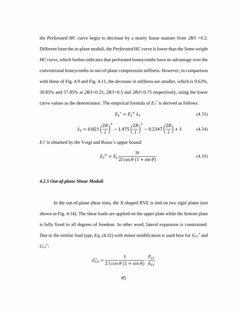
85

the Perforated HC curve begin to decrease by a nearly linear manner from 2R/l =0.2.

Different from the in-plane moduli, the Perforated HC curve is lower than the Same weight

HC curve, which further indicates that perforated honeycombs have no advantage over the

conventional honeycombs in out-of-plane compression stiffness. However, in comparison

with those of Fig. 4.9 and Fig. 4.11, the decrease in stiffness are smaller, which is 9.63%,

30.85% and 57.85% at 2R/l=0.25, 2R/l=0.5 and 2R/l=0.75 respectively, using the lower

curve values as the denominator. The empirical formula of E3* is derived as follows:

𝐸3∗ = 𝐸3

𝑢 𝜆3 (4.33)

𝜆3 = 0.821 (2𝑅

𝑙)

3

− 1.475 (2𝑅

𝑙)

2

− 0.2347 (2𝑅

𝑙) + 1 (4.34)

E3u is obtained by the Voigt and Reuss’s upper bound:

𝐸3𝑢 = 𝐸𝑠

3𝑡

2𝑙 cos 𝜃 (1 + sin 𝜃) (4.35)

4.2.5 Out-of-plane Shear Moduli

In the out-of-plane shear tests, the X-shaped RVE is tied on two rigid plates (not

shown in Fig. 4.14). The shear loads are applied on the upper plate while the bottom plate

is fully fixed in all degrees of freedom. In other word, lateral expansion is constrained.

Due to the similar load type, Eq. (4.32) with minor modification is used here for G13* and

G23*:

𝐺13∗ =

1

2 𝑙 𝑐𝑜𝑠 𝜃 (1 + 𝑠𝑖𝑛 𝜃)∙

𝑃13

𝛿13,

86

𝐺23∗ =

1

2 𝑙 𝑐𝑜𝑠 𝜃 (1 + 𝑠𝑖𝑛 𝜃)∙

𝑃23

𝛿23 (4.36)

where P13, P23, δ13 and δ23 are the RVE’s loads and deflections as marked in Fig. 9 (a) and

Fig. 9 (b).

Fig. 4.14. Deformation of the RVE under out-of-plane shear in the (a) X1-X3 direction

and (b) X2-X3 direction

Fig. 4.15. Out-of-plane shear moduli of perforated honeycombs vs. 2R/l

0

0.0004

0.0008

0.0012

0.0016

0.002

0 0.2 0.4 0.6 0.8 1

G1

3*/G

s(G

23

*/G

s )

2R/l

Perforated HC

Weight-normalized

Same weight HC

δ23

P23

P23

P13

δ13

P13

(a) (b)

87

Similar to E1* and E2

*, the FE simulations produces identical G13* and G23

* for

regular hexagonal honeycombs, as predicted by the existing analytical models [10,28].

Therefore, the two properties are plotted in the same graph as well. The curves in Fig. 4.15

shows that adding perforations on honeycomb cell walls has a negative effect on the

specific out-of-plane shear moduli. In this case, the Same weight HC curve is higher than

the Perforated HC curve by 10.83%, 48.37% and 175.34% at 2R/l=0.25, 2R/l=0.5 and

2R/l=0.75 respectively. Analytical calculations show that for honeycombs under out-of-

plane shear loads, the single cell walls’ planar shear contributes the majority of the strain

energy. Under this form of deformation, the stress of a cell wall will concentrate around

the two diagonal lines. However, the perforation blocks the stress transfer along the

diagonal lines and therefore greatly weakens the shear stiffness.

The empirical formulas for G13* and G23

* are given as:

𝐺13∗ = 𝐺13

𝑢 𝜆13,

𝐺23∗ = 𝐺23

𝑢 𝜆23 (4.37)

𝜆13 = 𝜆23 = 1.5876 (2𝑅

𝑙)

3

− 2.5699 (2𝑅

𝑙)

2

− 0.0304 (2𝑅

𝑙) + 1 (4.38)

where

𝐺13𝑢 =

𝑐𝑜𝑠 𝜃

(1 + 𝑠𝑖𝑛 𝜃)(

𝑡

𝑙) 𝐺𝑠 (4.39)

The calculation of G23u is more complicated compared to G13

u because it is found that G23u

is related to the aspect ratio of the cell wall. Here the empirical solution summarized by

Grediac, M. [28] is employed:

𝐺23𝑢 = 0.213 𝐺23𝑙𝑜𝑤𝑒𝑟

𝑢 + 0.787 𝐺23𝑢𝑝𝑝𝑒𝑟𝑢 (4.40)

88

where G23ulower and G23

uupper are the analytical lower and upper bounds [28]:

𝐺23𝑙𝑜𝑤𝑒𝑟𝑢 =

1 + 𝑠𝑖𝑛 𝜃

3 𝑐𝑜𝑠 𝜃(

𝑡

𝑙) 𝐺𝑠,

𝐺23𝑢𝑝𝑝𝑒𝑟𝑢 =

1 + 2 𝑠𝑖𝑛2 𝜃

2(1 + 𝑠𝑖𝑛 𝜃) 𝑐𝑜𝑠 𝜃(

𝑡

𝑙) 𝐺𝑠 (4.41)

Numerical method is still suggested by many authors to obtain the accurate solutions of

the out-of-plane shear moduli.

4.2.6 Out-of-plane Bending Rigidity

The out-of-plane bending of honeycombs is a collective effect of the twisting and

planar bending of the cell walls, and the twisting has been proven to be the dominant

mechanism [47]. Hence, a single cell wall instead of the X-shaped RVE is again used in

this analysis. From Chen’s work [32], the effective bending rigidities can be derived by

the cell wall edge twisting moment Mt and the cell wall twisting angle β through the

following equations:

𝐷1∗ = −

1

2

𝑐𝑜𝑠 𝜃

(1 + 𝑠𝑖𝑛 𝜃) 𝑠𝑖𝑛2 𝜃∙

𝑀𝑡

𝛽,

𝐷2∗ = −

1

2 (1 + 𝑠𝑖𝑛 𝜃)

𝑐𝑜𝑠3 𝜃∙

𝑀𝑡

𝛽,

𝐷12∗ = −

1

2

1

𝑠𝑖𝑛 𝜃 𝑐𝑜𝑠 𝜃∙

𝑀𝑡

𝛽 (4.42)

And the relationships between the external uniform moment �̅�1, �̅�2 and the external

bending curvature ρ1, ρ2 are given by Timoshenko [96]:

89

�̅�1 = 𝐷1∗

1

𝜌1+ 𝐷12

∗1

𝜌2,

�̅�2 = 𝐷2∗

1

𝜌2+ 𝐷12

∗1

𝜌1 (4.43)

Fig. 4.16. Deflection of an inclined cell wall under overall uniform out-of-plane bending

Fig. 4.17. Out-of-plane bending rigidities of perforated honeycombs vs. 2R/l

0

0.5

1

1.5

2

2.5

3

3.5

4

0 0.2 0.4 0.6 0.8 1

D1

*/E

sIs

(D2

*/E

sIs ,

D12

*/E

sIs)

2R/l

Perforated HC

Weight-normalized

Same weight HC

β

Mt

Mt

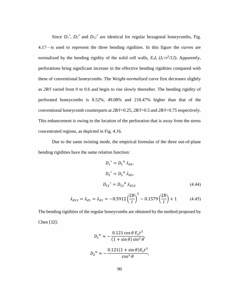
90

Since D1*, D2

* and D12* are identical for regular hexagonal honeycombs, Fig.

4.17—is used to represent the three bending rigidities. In this figure the curves are

normalized by the bending rigidity of the solid cell walls, EsIs (Is=t3/12). Apparently,

perforations bring significant increase in the effective bending rigidities compared with

these of conventional honeycombs. The Weight-normalized curve first decreases slightly

as 2R/l varied from 0 to 0.6 and begin to rise slowly thereafter. The bending rigidity of

perforated honeycombs is 8.52%, 49.08% and 218.47% higher than that of the

conventional honeycomb counterparts at 2R/l=0.25, 2R/l=0.5 and 2R/l=0.75 respectively.

This enhancement is owing to the location of the perforation that is away from the stress

concentrated regions, as depicted in Fig. 4.16.

Due to the same twisting mode, the empirical formulas of the three out-of-plane

bending rigidities have the same relation function:

𝐷1∗ = 𝐷1

𝑢 𝜆𝑑1,

𝐷2∗ = 𝐷2

𝑢 𝜆𝑑2,

𝐷12∗ = 𝐷12

𝑢 𝜆𝑑12 (4.44)

𝜆𝑑12 = 𝜆𝑑1 = 𝜆𝑑1 = −0.5912 (2𝑅

𝑙)

2

− 0.1579 (2𝑅

𝑙) + 1 (4.45)

The bending rigidities of the regular honeycombs are obtained by the method proposed by

Chen [32]:

𝐷1𝑢 ≈ −

0.121 cos 𝜃 𝐸𝑠𝑡3

(1 + sin 𝜃) sin2 𝜃,

𝐷2𝑢 ≈ −

0.121(1 + sin 𝜃)𝐸𝑠𝑡3

cos3 𝜃,

91

𝐷12𝑢 ≈ −

0.121𝐸𝑠𝑡3

𝑐𝑜𝑠 𝜃 sin 𝜃 (4.46)

4.2.7 Out-of-plane Critical Compressive Stress

In this and the next subsections, constant displacement are applied on the rigid

plates bounded to the RVE, and the reaction force on the rigid plates at the critical

displacement is extracted to calculate the effective critical stress. Two types of

honeycomb-skin connections—simply supported and clamped—are modeled to obtain the

lower and upper bounds of the critical stress. The first eigen buckling mode under these

two boundary conditions are shown in Fig. 4.18. From the curves plotted in Fig. 4.19, it is

observed that even without considering the weight, perforated honeycomb still

demonstrates enhanced critical stress compared to the conventional honeycombs. If the

weight is taken into consideration, such effect becomes even more significant. Taking

Perforated HC, clamped curve as an example, the perforated honeycomb has the critical

stress 16.30%, 92.66% and 474.91% higher than the Same weight HC, clamped curve at

2R/l=0.25, 2R/l=0.5 and 2R/l=0.75 respectively.

92

Fig. 4.18. First buckling mode of the RVE under out-of-plane compression with (a)

simply supported connection and (b) clamped connection.

Fig. 4.19. Out-of-plane compressive buckling stress of perforated honeycombs vs. 2R/l.

The critical buckling shape is the major cause for this drastic increase in buckling

resistance. The bending deformation of the first buckling mode shown in Fig. 4.18

accumulates quickly around the center of the plate to satisfy the smallest half wave

number. Since strain energy method indicates that bifurcation occurs when the work done

by the external force on the plate membrane becomes larger than the bending strain energy

0

1

2

3

4

5

6

7

8

9

10

0 0.2 0.4 0.6 0.8 1

σ3cr

*(M

Pa

)

2R/l

Perforated HC, Clamped

Weight-normalized, Clamped

Same weight HC, Clamped

Perforated HC, Simply supported

Weight-normalized, Simply supported

Same weight HC, Simply supported

P3

(a) (b)

P3

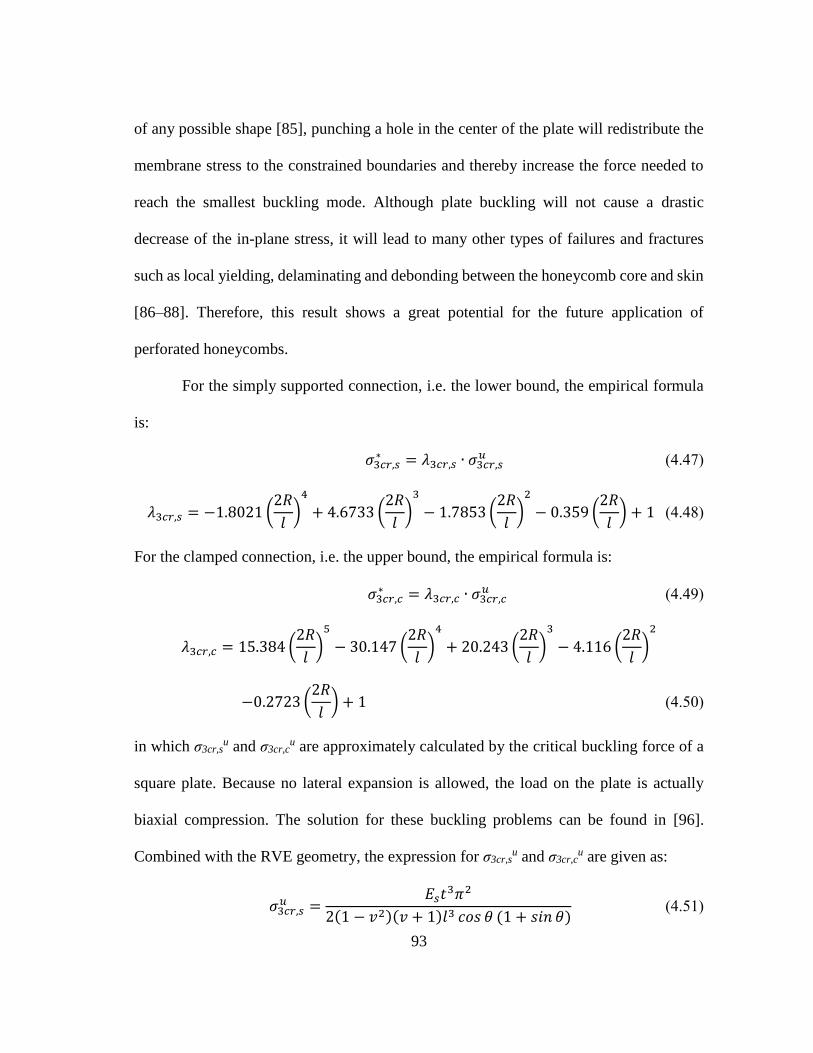
93

of any possible shape [85], punching a hole in the center of the plate will redistribute the

membrane stress to the constrained boundaries and thereby increase the force needed to

reach the smallest buckling mode. Although plate buckling will not cause a drastic

decrease of the in-plane stress, it will lead to many other types of failures and fractures

such as local yielding, delaminating and debonding between the honeycomb core and skin

[86–88]. Therefore, this result shows a great potential for the future application of

perforated honeycombs.

For the simply supported connection, i.e. the lower bound, the empirical formula

is:

𝜎3𝑐𝑟,𝑠∗ = 𝜆3𝑐𝑟,𝑠 ∙ 𝜎3𝑐𝑟,𝑠

𝑢 (4.47)

𝜆3𝑐𝑟,𝑠 = −1.8021 (2𝑅

𝑙)

4

+ 4.6733 (2𝑅

𝑙)

3

− 1.7853 (2𝑅

𝑙)

2

− 0.359 (2𝑅

𝑙) + 1 (4.48)

For the clamped connection, i.e. the upper bound, the empirical formula is:

𝜎3𝑐𝑟,𝑐∗ = 𝜆3𝑐𝑟,𝑐 ∙ 𝜎3𝑐𝑟,𝑐

𝑢 (4.49)

𝜆3𝑐𝑟,𝑐 = 15.384 (2𝑅

𝑙)

5

− 30.147 (2𝑅

𝑙)

4

+ 20.243 (2𝑅

𝑙)

3

− 4.116 (2𝑅

𝑙)

2

−0.2723 (2𝑅

𝑙) + 1 (4.50)

in which σ3cr,su and σ3cr,c

u are approximately calculated by the critical buckling force of a

square plate. Because no lateral expansion is allowed, the load on the plate is actually

biaxial compression. The solution for these buckling problems can be found in [96].

Combined with the RVE geometry, the expression for σ3cr,su and σ3cr,c

u are given as:

𝜎3𝑐𝑟,𝑠𝑢 =

𝐸𝑠𝑡3𝜋2

2(1 − 𝑣2)(𝑣 + 1)𝑙3 𝑐𝑜𝑠 𝜃 (1 + 𝑠𝑖𝑛 𝜃) (4.51)

94

𝜎3𝑐𝑟,𝑐𝑢 =

81𝐸𝑠𝑡3𝜋2

24(1 − 𝑣2)(3𝑙2𝑣 + 4𝑙2)𝑙 cos 𝜃 (1 + sin 𝜃) (4.52)

4.2.8 Out-of-plane Critical Shear Stress

The in-plane moduli E1* and E2

* are identical due to the planar isotropy of regular

hexagonal honeycombs, but the out-of-plane critical shear buckling stresses in the X1 and

X2 directions are different as a result of the different amounts of shear loads in cell walls

along different directions. In Fig. 4.20, when P13 is applied on the RVE, the cell wall along

the y-direction bears no in-plane shear load, hence the buckling initiates on the inclined

cell walls first. But when P23 is applied, the same cell wall bears half of the total shear

load, hence it will buckle before the inclined cell walls. However, since the buckling mode

of the different cell walls are identical, the shape of the τ13cr* and τ23cr

* curves are very

similar, as shown in Fig. 4.21 (a) and Fig. 4.21 (b). It is obvious that both the perforated

and unperforated honeycomb curves have decreased shear buckling stress as the

perforation radius increases, but the trend is slightly different. For all of the four loading

conditions (P13, P23; simply supported, clamped), the critical stresses of the conventional

honeycomb are initially larger than that of the perforated honeycomb, then the Same

weight HC curves fall below the Perforated HC curves when 2R/l exceeds some certain

values. However, from Fig. 4.21 it can be observed that the differences between these two

curves are not significant, so in general the perforation can be seen as having neutral effect

on the out-of-plane shear buckling resistance.

95

Fig. 4.20. First buckling mode of the RVE under out-of-plane shear loads. (a) X1-X3

shear with simply supported connection; (b) X2-X3 shear with simply supported

connection; (c) X1-X3 shear with clamped connection; (d) X2-X3 shear with clamped

connection.

P23

P23

P23

P23

(a) (b)

P13

P13

(d) (c)

P13

P13

96

Fig. 4.21. Out-of-plane critical shear stress of perforated honeycombs vs. 2R/l in the (a)

X1-X3 and (b)X2-X3 directions

From the buckling shapes illustrated in Fig. 4.20, it is found that the bulging

deformation formed an ellipse with its major axis coincides with one of the cell walls’

diagonal lines. In this case, the tensile stress along that diagonal line tends to obstruct the

out-of-the-plane deflection of the plate, but the perforation blocks the transfer of that

tensile stress and hence make the plate more prone to buckling. On the other hand, since

0

0.5

1

1.5

2

2.5

3

3.5

4

4.5

5

0 0.2 0.4 0.6 0.8 1

τ 23cr

*(M

Pa

)

2R/l

Perforated HC, clamped

Weight-normalized, clamped

Same weight HC, clamped

Perforated HC, simply supported

Weight-normalized, simply supported

Same weight HC, simply supported

(b)

0

1

2

3

4

5

6

0 0.2 0.4 0.6 0.8 1

τ 13cr

*(M

Pa

)

2R/l

Perforated HC, clamped

Weight-normalized, clamped

Same weight HC, clamped

Perforated HC, simply supported

Weight-normalized, simply supported

Same weight HC, simply supported

(a)

97

the compression stress along the other diagonal line facilitates the plate’s buckling, the

overall effect of the perforations on the shear buckling tends to be neutralized. Due to the

similar curve shape and identical buckling mode of the cell wall, is it found that the shear

buckling stresses in the two directions under the same edge connection (simply supported

or clamped) can be accurately expressed by one relation function, which means two

relation functions are needed in the four empirical formulas:

𝜏13𝑐𝑟,𝑠∗ = 𝜆13𝑐𝑟,𝑠𝜏13𝑐𝑟,𝑠

𝑢 ,

𝜏13𝑐𝑟,𝑐∗ = 𝜆13𝑐𝑟,𝑐𝜏13𝑐𝑟,𝑐

𝑢 ,

𝜏23𝑐𝑟,𝑠∗ = 𝜆23𝑐𝑟,𝑠𝜏23𝑐𝑟,𝑠

𝑢 ,

𝜏23𝑐𝑟,𝑐∗ = 𝜆23𝑐𝑟,𝑐𝜏23𝑐𝑟,𝑐

𝑢 (4.53)

𝜆13𝑐𝑟,𝑠 = 𝜆23𝑐𝑟,𝑠 = 0.9843 (2𝑅

𝑙)

3

− 0.4548 (2𝑅

𝑙)

2

− 1.2644 (2𝑅

𝑙) + 1 (4.54)

𝜆13𝑐𝑟,𝑐 = 𝜆23𝑐𝑟,𝑐 = 0.4234 (2𝑅

𝑙)

3

+ 0.0556 (2𝑅

𝑙)

2

− 1.1981 (2𝑅

𝑙) + 1 (4.55)

where τ13cr,s* and τ23cr,s

* are the lower bounds (simply supported) of critical shear buckling

stress in the X1-X3 and X2-X3 directions respectively, and τ13cr,c* and τ23cr,c

* are the upper

bounds (clamped) of critical shear buckling stress in the X1-X3 and X2-X3 directions

respectively. The critical shear stresses of the regular honeycombs are calculated from the

shear buckling coefficient of a square plate:

{𝜏13𝑐𝑟,𝑐

𝑢

𝜏13𝑐𝑟,𝑠𝑢 } = 𝑘𝑠

𝐸𝑠𝑡2𝜋2

12(1 − 𝑣2)𝑙2∙

𝑡

𝑙(1 + 𝑠𝑖𝑛 𝜃) (4.56)

{𝜏23𝑐𝑟,𝑐

𝑢

𝜏23𝑐𝑟,𝑠𝑢 } = 𝑘𝑠

𝐸𝑠𝑡2𝜋2

12(1 − 𝑣2)𝑙2∙

𝑡(1 + 2 𝑠𝑖𝑛2 𝜃)

2𝑙 𝑐𝑜𝑠 𝜃 (1 + 𝑠𝑖𝑛 𝜃) (4.57)

98

where ks is the shear buckling coefficient of a square plate. FE studies show that ks=11.15

and ks=13.52 for the lower bound and upper bound respectively.

It is noteworthy that although all of the empirical formulas derived in this section

are based on regular hexagonal honeycombs, they can also describe irregular hexagonal

honeycombs (θ≠30°) since the cell wall angle factor is included in the conventional

honeycomb properties like E1u.

4.3 Experimental Verification

To verify the derived empirical formulas, a series of perforated honeycomb

specimens were fabricated through 3D printing (EOS P 396 selective laser sintering

printer, EOS of North America Inc, Novi, MI) from nylon powders. The designed size

parameters of these specimens are: l=16mm, t=0.7mm, θ=30°. Specimens of three

perforation sizes—2R/l=0.25, 2R/l=0.5 and 2R/l=0.75— are printed, as shown in Fig. 4.22

from left to right. Each design has two replicates, which are labeled as A and B in the

following graphs. Pre-tests were carried out on three solid cubic parts printed in the same

batch to measure the modulus of the printed bulk. The results showed that the printed

material has almost isotropic elastic modulus of 943 MPa. Due to the coarse surface

generated from during sintering, the actual working thickness is less than the designed

thickness. Thus, another two tests were conducted on two conventional honeycomb

specimens, and the actual working thickness is calculated by substituting the measured

stress-strain slope into Gibson and Ashby’s analytical honeycomb model. It was found

99

that for the designed thickness of 0.7mm, the actual working thickness is 0.62mm. The

real modulus and thickness obtained above are used in the calculation of the empirical

solutions that are compared to the test results.

Compression tests in the X1, X2 and X3 directions were conducted on the perforated

honeycomb specimens. The tests were operated according to ASTM C364/C364M test

standard for sandwich core edgewise compressive properties and C365/C365M test

standard for sandwich core flatwise compressive properties. For the in-plane (edgewise)

tests, a special fixture was made according to the ASTM standard to prevent the

specimen’s flatwise deflection, as shown in Fig. 4.23 (a). The fixture has a loose fit with

the specimens, and the contacting surfaces were polished to reduce the friction that

hampers the specimens’ lateral expansion. For the out-of-plane (edgewise) tests, the

specimens were not bonded onto the platens because any adhesive that is strong enough

to form clamped boundary condition (constrain the edge rotations) will generate non-

negligible property change on the adjacent material. Instead, two 1000 grit sandpapers

were adhered on the upper and lower platens to approximate the simply supported non-

expansion boundary condition, as shown in Fig. 4.23 (b). The tests were performed on a

MTS insight screw driven mechanical test machine. The head displacement rates were

1mm/min and 0.5mm/min for the in-plane and out-of-plane compression tests

respectively. For the out-of-plane compression test, the process was video recorded to

capture the moment of onset of buckling onset, so that the corresponding load force can

be obtained from the exported test data. The reason for using this method is because

100

usually there is no significant slope change on the stress-strain curve that can be identified

as buckling [97].

Fig. 4.22. 3D Printed perforated honeycomb specimens with 2R/l=0.25, 2R/l=0.5 and

2R/l=0.75, from left to right.

Fig. 4.23. Experiment setups for (a) in-plane (edgewise) compression tests and (b) out-

of-plane compression tests.

4.4 Results and Discussion

In this part, the in-plane elastic moduli and out-of-plane compressive buckling

stress obtained from the analytical model, empirical formulas and experimental tests are

compared and discussed. Since the empirical formulas provide almost identical results

2R/l=0.2

5

2R/l=0.5 2R/l=0.75

(a) (b)

101

with those of the finite element simulations (recall that the maximum difference is less

than 1%), numerical studies that repeats the experimental tests are not conducted.

In Fig. 4.24, the experimental results of the in-plane effective moduli E1* and E2

*

are compared with the analytical solutions calculated from Eq. (4.1) to (4.12) and the

empirical formulas in Eq. (4.25) to (4.27). As mentioned in Section 4.1, two different

methods are used to derive the analytical in-plane elastic moduli for honeycombs with

small perforation and large perforation respectively, and 2R/l=0.52 is the dividing point

of using the two solutions. It is obvious that the two analytical solutions are very accurate

when 2R/l is close 0 or 1, but they show a relative large deviation around the dividing

point, at which the analytical result is 16.72% higher than the empirical result. The

solutions obtained by the effective width method is also plotted in Fig. 4.24 as the dot-

dashed line. It can be seen that through the whole domain, the empirical results agree better

with the experimental data than the analytical results. The effective width method also

shows a good prediction, but the curve trend at 2R/l > 0.5 doesn’t match the experimental

data very well. Besides, all of the empirical and analytical solutions tend to overestimate

the effective in-plane modulus at large 2R/l values. The major reasons for this difference

is the size of the specimen. The RVE used in the finite element simulations aims to model

an infinite honeycomb panel, but the outer cell walls of the specimens are less constrained

than the inner cell walls, which makes the specimens less stiff under compression.

102

Fig. 4.24. Graphical comparison of analytical, empirical and experimental results of in-

plane elastic moduli.

In Fig. 4.25, the buckling stresses of the specimens under the X3-direction load are

plotted and compared with the upper and lower bounds calculated from the analytical

model stated in Eq. (4.13) to (4.20) and the empirical formulas stated in Eq. (4.47) to

(4.52). Although there is no bonding between the honeycombs and the compression

platens, the cell walls’ free rotation at their contacting edges is still hindered due to the

non-negligible cell wall thickness, which leads to an anti-rotation moment about the

middle plane. Hence, the real cell walls’ constraint is between simply supported and

clamped condition, and this condition agrees with the data distribution of the first three

points shown in Fig. 4.25. Form this figure it can be seen that the analytical upper and

lower bounds buckling stress have a good agreement with the experimental and empirical

0

0.02

0.04

0.06

0.08

0.1

0.12

0.14

0.16

0.18

0.2

0 0.2 0.4 0.6 0.8 1

E1*, E

2*

(MP

a)

2R/l

Empirical formula resultsAnalytical solution of small perforationAnalytical solution of large perforationEffective width methodE1*, specimen AE1*, specimen BE2*, specimen AE2*, specimen B

2R/l=0.52

103

results in most of the domain. At large 2R/l ratio, the approximate Rayleigh-Ritz method

leads to a sharply increased buckling stress, which is due to the different eigen buckling

mode, as discussed in the end of Section 4.1.3. For the first three 2R/l values, the

experimental results do not strictly follow the decrease-increase trend of the analytical and

empirical curves, but remained broadly unchanged. In the aspect of unit weight buckling

resistance, this result confirmed that honeycombs with perforated cell walls have

improved specific buckling stress compared with the conventional honeycombs with the

same relative density. At 2R/l=0.75, in contrast to the increased analytical and empirical

curves, the experimental results decreased steeply and fell below the two lower bounds.

Observing the shape of the deformed specimens, two causes are found for this significant

difference. The first cause is the finite specimen size. For large 2R/l ratios, the cell wall

behaves more like two independent columns with varying cross-sections. The inner

columns with three jointed cell walls can maintain a straight center line at a very high

compression load, but the outer columns (around the perimeter of the specimen) with only

two jointed cell walls tend to bend outward at a relatively small load. The second cause is

the buckling mode change. It is observed that, when the compression load exceeded a

certain value, the 2R/l=0.75 specimens generated a slight horizontal relative displacement

between its upper and lower surfaces, which made the buckling mode shifted from axial

buckling (Fig. 4.18) to shear buckling (Fig. 4.20), which has a much lower buckling

coefficient at a large perforation size. For this reason, perforations with 2R/l>0.5 are not

recommended for the purpose of improving buckling resistance. However, this criterion

is less critical for large honeycomb panels.

104

Fig. 4.25. Graphical comparison of analytical, empirical and experimental results of the

homogenized out-of-plane critical stress.

In spite of the difference between the empirical and experimental buckling stresses, it

is important that the finite element simulations conducted on the RVE can predict the

buckling modes of the cell walls, as shown in Fig. 4.26. In both approaches, there is one

half-wave buckling on each cell wall and the bulging out directions of the cell walls are

barreling about the center axes of the cell wall joints.

0

0.05

0.1

0.15

0.2

0.25

0.3

0.35

0.4

0.45

0.5

0 0.2 0.4 0.6 0.8 1

σ3cr

*(M

Pa

)

2R/l

Empirical upper bound

Empirical lower bound

Analytical upper bound

Analytical lower bound

Specimen A

Specimen B

105

Fig. 4.26. The buckling modes of the deformed specimens and the RVE with (a)

2R/l=0.25, (b) 2R/l=0.5, (c) 2R/l=0.75

4.5 Conclusions

A numerical and experimental study is carried out to investigate and summarize

the mechanical behaviors of a new type of honeycombs with perforated cell walls. FE

simulations are conducted on a RVE with periodic boundary conditions, and the empirical

formulas for the homogenized moduli, bending rigidities and critical buckling stresses are

derived based on the FEA results. A series of specimens were fabricated by 3D printing,

and their compressive responses were tested and compared with those obtained from the

empirical formulas.

To summarized the influence of the perforations, the percentage change of the

properties of the perforated honeycombs with respect to the conventional honeycombs of

(a) (b) (c)

2R/l=0.25 2R/l=0.5 2R/l=0.75

106

the same relative density at three 2R/l ratios are listed in Table 4.3. A positive percentage

indicates an improved property by the perforations and vice versa. The results show that

adding perforations on the cell walls increases the in-plane moduli, bending rigidities, and

out-of-plane compressive buckling resistance; but it decreases the out-of-plane moduli.

For the out-of-plane shear buckling resistance, perforations have in general a nearly

neutral effect. The in-plane and out-of-plane compression tests conducted on the 3D

printed specimens verified the empirical in-plane moduli, but revealed that the buckling

mode of the honeycombs with large perforation sizes is likely to shift from compressive

buckling to shear buckling, which leads to a much lower buckling stress than the numerical

results. Based on this fact, a 2R/l ratio smaller than 0.6 is suggested to obtain the

maximized buckling resistance per unit weight for small honeycomb panels. These

property enhancements show potentials for the perforated honeycombs to be utilized in

real products based on the requirements of the specific applications.

107

Table 4.3. Properties change brought by the perforations at three 2R/l ratios

Stress concentration around the perforations is not investigated in this part of work,

but it can be an important factor to determine the real failure mode—for large holes the

cell walls may yield first instead of buckle. The issue is material and thickness related and

should be studied case by case.

2R/l 0.25 0.5 0.75

E1*, E2

*, G12* 16.2% 92.7% 474.9%

E3* -8.8% -23.6% -36.7%

G13*, G23

* -9.8% -32.6% -63.7%

D1*, D2

*, D12* 8.5% 49.1% 218.5%

σ3cr,s * -1.0% 62.6% 540.0%

σ3cr,c * 16.3% 92.7% 474.9%

τ13cr,s* -20.1% -27.0% -43.4%

τ13cr,c* -16.7% -10.0% 86.4%

108

5. SUMMARY AND FUTURE WORK

In this work, three novel honeycombs with modified cell walls are proposed and

investigated in three corresponding parts.

The first part provides the analytically homogenized stiffness matrix of

honeycombs with spline-shaped cell walls. This new model is proven to be accurate in

describing a wide range of 2-D periodic structures with non-linear cell walls. Based on the

parametric study results, cell wall design strategies are suggested for maximizing the in-

plane moduli and out-of-plane buckling resistance of this honeycomb. For future work,

further research is suggested to model the out-of-plane buckling stress by examining into

the range of the spline function’s curvature that allows low eigenvalue buckling modes to

occur. The spline cell walls with more control points can also be studied to obtain higher

specific stiffness and specific strength.

The second part proposes a novel honeycomb with laminated composite cell walls.

The analytically homogenized stiffness matrix for this new honeycomb is derived and

verified numerically. Parametric study shows that the homogenized in-plane moduli

change non-linearly with the ply thickness ratio—a small thickness of the stiffer ply can

bring a large increase in the effective moduli. To further explore the potential of this type

of honeycombs, their collapse process can be investigated in the future. In addition to the

plastic failure as that of the conventional honeycombs, the composite cell walls can also

delaminate. Such failure can greatly change the stress-strain response during the

collapsing process.

109

The third part proposes a novel honeycomb with centric circular perforations on

its square cell walls. An X-shaped representative volume element with periodic boundary

conditions is built for finite element analysis to investigate the influence of the perforation

size on the homogenized stiffness and buckling stress. It is observed that these perforations

can greatly improve some of the properties at a unit weight. Empirical formulas are derived

from the numerical results to predict the behavior of this honeycomb. Future work can

include the investigation of the stress concentration around the perforations under different

loads, and how the perforation changes the failure mode of honeycombs. Mechanical

behaviors of honeycombs with rectangular cell walls and multiple perforations on one cell

wall can also be considered in the next stage of this research.

110

REFERENCES

[1] Gibson LJ, Ashby MF. Cellular solids: Structure and properties. Cambridge:

Canbridge University Press, 1999

[2] Sarikaya M, Gunnison KE, Yasrebi M, Aksay IA. Mechanical Property-

microstructural relationships in abalone shell. Mater Reseaerch Soc Symp

1990;174:109–116.

[3] Jain S, Kumar R, Jindal UC. Mechanical behaviour of bamboo and bamboo

composite. J Mater Sci 1992;27:4598–4604.

[4] Wang A-J, McDowell DL. In-plane stiffness and yield strength of periodic metal

honeycombs. J Eng Mater Technol 2004;126:137–156.

[5] Kintscher M, Karger L, Wetzel A, Hartung D. Stiffness and failure behaviour of

folded sandwich cores under combined transverse shear and compression.

Compos Part A Appl Sci Manuf 2007;38:1288–1295.

[6] Nilsson E, Nilsson Ac. Prediction and measurement of some dynamic properties

of sandwich structures with honeycomb and foam cores. J Sound Vib

2002;251:409–430.

[7] Petras a., Sutcliffe MPF. Failure mode maps for honeycomb sandwich panels.

Compos Struct 1999;44:237–252.

[8] Xu XF, Qiao P, Davalos JF. Transverse shear stiffness of composite honeycomb

core with general configuration. J Eng Mech 2001;127:1144 –1156.

[9] Frank Xu X, Qiao P. Homogenized elastic properties of honeycomb sandwich

with skin effect. Int J Solids Struct 2002;39:2153–2188.

111

[10] Wadley HNG. Multifunctional periodic cellular metals. Philos Trans R Soc A

Math Phys Eng Sci 2006;364:31–68.

[11] Hohe J, Becker W. Effective stress-strain relations for two-dimensional cellular

sandwich cores: Homogenization, material models, and properties. Appl Mech

Rev 2002;55:61.

[12] Olympio KR, Gandhi F. Flexible skins for morphing aircraft using cellular

honeycomb cores. J Intell Mater Syst Struct 2010;21:1719–1735.

[13] Dale AS, Cooper JE, Mosquera A. Topology optimization & experimental

validation of 0-ν honeycomb for adaptive morphing wing. 22nd

AIAA/ASME/AHS Adaptive Structrures Conference, National Harbor, Maryland,

2014.

[14] Olympio KR, Gandhi F. Zero poisson’s ratio cellular honeycombs for flex skins

undergoing one-dimensional morphing. J Intell Mater Syst Struct 2010; 21:1737–

1753.

[15] Ju J, Kim DM, Kim K. Flexible cellular solid spokes of a non-pneumatic tire.

Compos Struct 2012;94:2285–2295.

[16] Hu L, You F, Yu T. Effect of cell-wall angle on the in-plane crushing behaviour

of hexagonal honeycombs. Mater Des 2013;46:511–523.

[17] Ruan D, Lu G, Wang B, Yu TX. In-plane dynamic crushing of honeycombs - A

finite element study. Int J Impact Eng 2003;28:161–182.

[18] Papka SD, Kyriakides S. In-plane compressive response and crushing of

honeycomb. J Mech Phys Solids 1994;42:1499–1532.

[19] Daryabeigi K. Heat transfer in adhesively bonded honeycomb core panels. J

Thermophys Heat Transf 2002;16:217–221.

112

[20] Lu TJ. Heat transfer efficiency of metal honeycombs. Int J Heat Mass Transf

1998;42:2031–2040.

[21] Huang WC, Ng CF. Sound insulation improvement using honeycomb sandwich

panels. Appl Acoust 1998;53:163–177.

[22] Davis EB. Designing honeycomb panels for noise control. Am Institue Aeronaut

Astronaut 1999:792–801.

[23] Grosveld FW, Mixson JS. Noise transmission through an acoustically treated and

honeycomb stiffened aircraft sidewall. J Aircr 1984;22:434–440.

[24] Ruzzene M. Vibration and sound radiation of sandwich beams with honeycomb

truss core. J Sound Vib 2004;277:741–763.

[25] Wilson S. A new face of aerospace honeycomb. Mater Des 1990;11:323–326.

[26] Masters IG, Evans KE. Models for the elastic deformation of honeycombs.

Compos Struct 1996;35:403–422.

[27] Kelsey S, Gellatly RA, Clark BW. The shear modulus of foil honeycomb cores: a

theoretical and experimental investigation on cores used in sandwich construction.

Aircr Eng Aerosp Technol 1958;30:294–302.

[28] Grediac M. A finite element study of the transverse shear in honeycomb cores. Int

J Solids Struct 1993;30:1777–1788.

[29] Penzien J, Didriksson T. Effective shear modulus of honeycomb cellular structure.

AIAA J 1964;2:531–535.

[30] Shi G, Tong P. Equivalent transverse shear stiffness of honeycomb cores. Int J

Solids Struct 1995;32:1383–1393.

[31] Pan SD, Wu LZ, Sun YG. Transverse shear modulus and strength of honeycomb

113

cores. Compos Struct 2008;84:369–374.

[32] Chen DH. Bending deformation of honeycomb consisting of regular hexagonal

cells. Compos Struct 2011;93:736–746.

[33] Chen DH. Equivalent flexural and torsional rigidity of hexagonal honeycomb.

Compos Struct 2011;93:1910–1917.

[34] Hohe J, Becker W. Effective elastic properties of triangular grid structures.

Compos Struct 1999;45:131–145.

[35] Hohe J, Becker W. An energetic homogenisation procedure for the elastic

properties of general cellular sandwich cores. Compos Part BEngineering

2001;32:185–197.

[36] Hohe J, Beschorner C, Becker W. Effective elastic properties of hexagonal and

quadrilateral grid structures. Compos Struct 1999;46:73–89.

[37] Qiao PZ, Wang JL. Mechanics of composite sinusoidal honeycomb cores. J

Aerosp Eng 2005;18:42–50.

[38] Li YM, Hoang MP, Abbes B, Abbes F, Guo YQ. Analytical homogenization for

stretch and bending of honeycomb sandwich plates with skin and height effects.

Compos Struct 2015;120:406–416.

[39] Burlayenko VN, Sadowski T. Effective elastic properties of foam-filled

honeycomb cores of sandwich panels. Compos Struct 2010;92:2890–2900.

[40] Sadowski T, Bȩc J. Effective properties for sandwich plates with aluminium foil

honeycomb core and polymer foam filling - Static and dynamic response. Comput

Mater Sci 2011;50:1269-1275.

[41] Catapano A, Montemurro M. A multi-scale approach for the optimum design of

sandwich plates with honeycomb core. Part I: Homogenisation of core properties.

114

Compos Struct 2014;118:664–676.

[42] Catapano A, Montemurro M. A multi-scale approach for the optimum design of

sandwich plates with honeycomb core. Part II: The optimisation strategy. Compos

Struct 2014;118:677–690.

[43] McFarland Jr. RK. Hexagonal cell structures under post-buckling axial load.

AIAA J 1963;1:1380–1385.

[44] Wierzbicki T. Crushing analysis of metal honeycombs. Int J Impact Eng

1983;1:157–174.

[45] Timoshenko SP, Gere J. Theory of elastic stability. Stanford: Dover Publications,

2009.

[46] Zhang J, Ashby MF. The out-of-plane properties of honeycombs. Int J Mech Sci

1992;34:475–489.

[47] Aktay L, Johnson AF, Kroplin BH. Numerical modelling of honeycomb core

crush behaviour. Eng Fract Mech 2008;75:2616–2630.

[48] Wilbert A, Jang WY, Kyriakides S, Floccari JF. Buckling and progressive

crushing of laterally loaded honeycomb. Int J Solids Struct 2011;48:803–816.

[49] López Jiménez F, Triantafyllidis N. Buckling of rectangular and hexagonal

honeycomb under combined axial compression and transverse shear. Int J Solids

Struct 2013;50:3934–3946.

[50] Ju J, Summers JD, Ziegert J, Fadel G. Design of honeycombs for modulus and

yield strain in shear. J Eng Mater Technol 2012;134:011002.

[51] Hou S, Ren L, Dong D, Han X. Crashworthiness optimization design of

honeycomb sandwich panel based on factor screening. J Sandw Struct Mater

2012;14:655–678.

115

[52] Singh G, Hopkins JB. General selection of lattice shape in ductile-reinforced

brittle structures for increased stiffness. Compos Struct 2015;131:325–332.

[53] Chen A, Davalos JF. A solution including skin effect for stiffness and stress field

of sandwich honeycomb core. Int J Solids Struct 2005;42:2711–2739.

[54] Chen Q, Pugno N, Zhao K, Li Z. Mechanical properties of a hollow-cylindrical-

joint honeycomb. Compos Struct 2014;109:68–74.

[55] Karnessis N, Burriesci G. Uniaxial and buckling mechanical response of auxetic

cellular tubes. Smart Mater Struct 2013;22:084008.

[56] Ajdari A, Jahromi BH, Papadopoulos J, Nayeb-Hashemi H, Vaziri A. Hierarchical

honeycombs with tailorable properties. Int J Solids Struct 2012;49:1413–1419.

[57] Sun Y, Pugno NM. In plane stiffness of multifunctional hierarchical honeycombs

with negative Poisson’s ratio sub-structures. Compos Struct 2013;106:681–689.

[58] Taylor CM, Smith CW, Miller W, Evans KE. The effects of hierarchy on the in-

plane elastic properties of honeycombs. Int J Solids Struct 2011;48:1330–1339.

[59] Alderson A, Alderson KL, Chirima G, Ravirala N, Zied KM. The in-plane linear

elastic constants and out-of-plane bending of 3-coordinated ligament and

cylinder-ligament honeycombs. Compos Sci Technol 2010;70:1034–1041.

[60] Scarpa F, Blain S, Lew T, Perrott D, Ruzzene M, Yates JR. Elastic buckling of

hexagonal chiral cell honeycombs. Compos Part A Appl Sci Manuf 2007;38:280–

289.

[61] Lakes R. Materials with structural hierarchy. Nature 1993;361:511–515.

[62] Ajdari A, Jahromi BH, Papadopoulos J, Nayeb-Hashemi H, Vaziri A. Hierarchical

honeycombs with tailorable properties. Int J Solids Struct 2012;49:1413–1419.

116

[63] Oftadeh R, Haghpanah B, Vella D, Boudaoud A, Vaziri A. Optimal fractal-like

hierarchical honeycombs. Phys Rev Lett 2014;113:104301.

[64] Chen Q, Pugno NM. In-plane elastic buckling of hierarchical honeycomb

materials. Eur J Mech A/Solids 2012;34:120–129.

[65] Sun Y, Chen Q, Pugno N. Elastic and transport properties of the tailorable

multifunctional hierarchical honeycombs. Compos Struct 2014;107:698–710.

[66] Mousanezhad D, Ebrahimi H, Haghpanah B, Ghosh R, Ajdari A, Hamouda AMS,

et al. Spiderweb honeycombs. Int J Solids Struct 2015;66:218–227.

[67] Larsen UD, Sigmund O, Bouwstra S. Design and fabrication of compliant

micromechanisms and structures with negative Poisson’s ratio. J

Microelectromechanical Syst 1997;6:99–106.

[68] Ko WL. Elastic Constants for Superplastically Formed/ Diffusion-Bonded

Sandwich Structures 1979;18:986–987.

[69] Fan HL, Jin FN, Fang DN. Mechanical properties of hierarchical cellular

materials. Part I: Analysis. Compos Sci Technol 2008;68:3380–3387.

[70] Yu W, Davis CS. Buckling behavior and post-buckling strength of perforated

stiffened compression elements. 1st International Specialty Conference on Cold-

Formed Steel Structures, Rolla, Missouri, 1970.

[71] Roberts TM, Azizian ZG. Strength of perforated plates subjected to in-plane

loading. Thin-Walled Struct 1984;2:153–164.

[72] Schlack AL. Elastic stability of pierced square plates. Experimental Mechanics

1964;4(6):167–172.

[73] Schlack AL. Experimental critical loads for perforated square plates.

Experimental Mechanics 1968;8(2):69–74.

117

[74] Levy BS, Woolley RM, Kroll WD. Instability of simply supported square plate

with reinforced circular hole in edge compression. Journal of Research 1947;571-

577

[75] Nemeth MP, Stein M, Johnson ER. An approximate buckling analysis for

rectangular orthotropic plates with centrally located cutouts. National Aeronautics

and Space Administration Hampton va Langley Research Center, 1986.

[76] Maiorana E, Pellegrino C, Modena C. Elastic stability of plates with circular and

rectangular holes subjected to axial compression and bending moment. Thin-

Walled Struct 2009;47:241–255.

[77] Aydin Komur M, Sonmez M. Elastic buckling of rectangular plates under linearly

varying in-plane normal load with a circular cutout. Mech Res Commun

2008;35:361–371.

[78] Aydin Komur M, Sonmez M. Elastic buckling behavior of rectangular plates with

holes subjected to partial edge loading. J Constr Steel Res 2015;112:54–60.

[79] de Vasconcellos Real M, Isoldi LA, Damas AP, Helbig D. Elastic and elasto-

plastic buckling analysis of perforated steel plates. VETOR-Revista de Ciências

Exatas e Engenharias 2013;23(2):61-70.

[80] El-Sawy KM, Nazmy AS. Effect of aspect ratio on the elastic buckling of

uniaxially loaded plates with eccentric holes. Thin-Walled Struct 2001;39:983–

998.

[81] El-Sawy KM, Nazmy AS, Martini MI. Elasto-plastic buckling of perforated plates

under uniaxial compression. Thin-Walled Struct 2004;42:1083–1101.

[82] El-Sawy KM, Ikbal Martini M. Elastic stability of bi-axially loaded rectangular

plates with a single circular hole. Thin-Walled Struct 2007;45:122–133.

118

[83] Nemeth MP. Buckling behavior of compression-loaded symmetrically laminated

angle-ply plates with holes. AIAA J 1988;26:330–336.

[84] Larsson PL. On buckling of orthotropic stretched plates with circular holes.

Compos Struct 1989;11:121–134.

[85] Rockey K, Narayanan R. Ultimate load capacity of plate girders with webs

containing circular cut-outs. ICE Proc 1981;71:845–862.

[86] Narayanan R, Chow FY. Ultimate capacity of uniaxially compressed perforated

plates. Thin-Walled Struct 1984;2:241–264.

[87] Narayanan R DI. Strength of slender webs having non-central holes. Struct Eng

Part B 1985:57–62.

[88] Shanmugam NE, Thevendran V, Tan YH. Design formula for axially compressed

perforated plates. Thin-Walled Struct 1999;34:1–20.

[89] Shanmugam NE, Dhanalakshmi M. State-of-art review and compilation of studies

on perforated thin-walled structures. Int J Struct Stab Dyn 2001;1:59–81.

[90] Hegarty RF, Ariman T. Elasto-dynamic analysis of rectangular plates with

circular holes. Int J Solids Struct 1975;11:895–906.

[91] Lo CC, Lessian AW. Bending of plates with circular holes. Acta Mechanica

1967;4:64-78.

[92] Le Fort P. Bending of perforated plates with square penetration patterns. Nucl

Eng Des 1970;12:122–134.

[93] Bailey RW, Hicks R. Behaviour of perforated plates under plane stress. J Mech

Eng Sci 1960;2:143–165.

[94] Hoffman RE, Ariman T. Thermal bending of plates with circular holes. Nucl Eng

119

Des 1970;14:231–238.

[95] Osama Bedair. Stress analyses of deep plate girders used at oil and gas facilities

with rectangular web penetrations. Pract Period Struct Des Constr 2011;16:73–81.

[96] Timoshenko, Stephen P. and SW-K. Theory of plates and shells. New York:

McGraw-hill Book Company; 1959.

[97] Miller W, Smith CW, Scarpa F, Evans KE. Flatwise buckling optimization of

hexachiral and tetrachiral honeycombs. Compos Sci Technol 2010;70:1049–1056.