Descriptive Statistics - Harvard University · Quantile(quartile, quintile, percentile, etc.): 25...

Descriptive Statistics

Kosuke Imai

Department of PoliticsPrinceton University

Fall 2011

Kosuke Imai (Princeton University) Descriptive Statistics POL345 Lectures 1 / 45

Variables and their Types

Variables: characteristics about each unit which takedifferent values across unitsQuantitative variables

Continuous: income, age, etc.Discrete: number of siblings, etc.Continuous variables may be measured discretely

Qualitative (Categorical) variablesstate, country, race, gender, party, etc.Nominal vs. Ordinal

In R,quantitative variable as a numeric objectqualitative variable as a factor object

Common data format:comma separated values (csv)other delimiter-separated values format; space, tab


Measurement Error

Variables must be measuredBut often they are measured with errorREADING: FPP Chapter 6

Random (chance) measurement errorNo bias: on average, there is no errorRepeated measurements: “Law of large numbers” which wewill cover later

Systematic measurement errorgovernment statistics in some countriesmis-reporting in surveys (social desirability bias)interpersonal incompatibility in surveys


Measuring the US Turnout Rate

Question: How do you measure turnout rate?Numerator: Total votes cast

Votes for highest office (president; governor or senator inmidterm elections)

Denomenator: VAP vs. VEPVAP from Census (adjustments for non-Census years)VEP = VAP + overseas voters − ineligible votersoverseas voters: military personnel and civiliansineligible voters: non-citizens, disenfranchised felons, mentalincompetents, those who failed to meet states’ residencyrequirement


VAP and VEP Turnout Rates are DifferentTrend graph

through 1948 is strikingly similar to the turnout rateafter 1972. The highs in the 1950s and 1960s areactually quite unusual for the period after the weaken-ing of political machines (Burnham 1987) and perhapswere more momentary than usually supposed.

The Twenty-Sixth Amendment. The drop in turnoutbetween 1968 and 1972 is usually attributed to expan-sion of the franchise from age 21 to age 18 (Rosenstoneand Hansen 1993, 57).4 This is a plausible assumption,since turnout rates for younger persons are lower thanfor older persons. Table 1 shows the turnout rateexcluding persons under age 21. The numerator isderived by using the CPS figures to calculate theproportion of all votes reported by persons age 21 andolder, and then multiplying that proportion by the totalnumber of votes cast for highest office; the denomina-tor is derived by removing the number of citizens age18–20 from the VEP (see the Appendix). The averageeffect of removing this group since 1971 is an increaseof 1.3 percentage points in presidential elections and1.7 percentage points in congressional elections. Thatis slightly more than one-fourth the decrease of 4.7percentage points for the VEP turnout rate between1948–68 and 1972–2000. Because a large drop in voterparticipation occurred between 1968 and 1972, it isassumed that the new voters were a significant factor inthe decline. Yet, the downward trend of the 1960scarries through to the 1972 election even thoughpeople age 18–20 are not included prior to 1972. Andthe turnout rate of voters under age 21 was 49.2% in

1972, according to the CPS, so their presence in thatelection only lowered the rate by a single percentagepoint.

Southern and Nonsouthern Turnout Rates. We need toaccount for the dramatic rise in southern turnout ratesduring the 1960s to make comparisons of the aggregateturnout rate over time. The civil rights movement ledto the Voting Rights Act, which effectively enfran-chised blacks and poor whites in the South. Accord-ingly, voter participation rose dramatically in thatregion during the 1960s (Kousser 1999).

The increase in southern turnout masks some of thedecline in the rest of the nation. The correctionsperformed in Table 1 are repeated in tables 2 and 3 fornonsouthern and southern states, respectively. Figure 2plots the national, southern, and nonsouthern age 21�VEP turnout rate for presidential elections since 1948,thereby controlling for the effects of the extendedfranchise and the elimination of Jim Crow laws. Turn-out rates in the South rose precipitously as the elector-ate mobilized, but elsewhere the electorate contracted(DeNardo 1998).5

Nationally and regionally, using either VAP or VEPin the denominator of the turnout rate, there are twodistinct eras of post–World War II turnout divided by1971. The national VAP presidential turnout rate is an

4 Before 1971, four states allowed persons under age 21 to vote:Georgia since 1944 (18�), Kentucky since 1956 (19�), Alaska since1960 (19�), and Hawaii since 1960 (20�) (GAO 1997).

5 Southern states are Alabama, Arkansas, Florida, Georgia, Louisi-ana, Mississippi, North Carolina, South Carolina, Texas, and Vir-ginia. The contribution of the southern turnout rate to the nationalfigure increased over the last half of the twentieth century. In 1960,approximately one in four eligible voters resided in the South. Asin-migration to that region increased, the number rose to almost oneout of three in 1996. Thus, decline in nonsouthern voter participationis offset by the shift in distribution of eligible voters across regions.

FIGURE 1. National VAP and VEP Presidential Turnout Rates, 1948–2000

American Political Science Review Vol. 95, No. 4

967

McDonald and Popkin (2001) American Political Science ReviewKosuke Imai (Princeton University) Descriptive Statistics POL345 Lectures 5 / 45

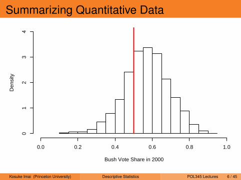
Summarizing Quantitative Data

Bush Vote Share in 2000

Den

sity

0.0 0.2 0.4 0.6 0.8 1.0

01

23

4


How to Read Histograms

READING: FPP Chapter 3

What is density scale?The areas of the blocks sum to 1 or 100%Density scale 6= Percentage (e.g., range 6= [0,1])The height of the blocks equals the percentage divided byclass interval lengthIn this case, “percent per vote share”Or more generally, “percentage per horizontal unit”


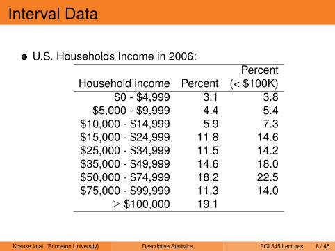
Interval Data

U.S. Households Income in 2006:Percent

Household income Percent (< $100K)$0 - $4,999 3.1 3.8

$5,000 - $9,999 4.4 5.4$10,000 - $14,999 5.9 7.3$15,000 - $24,999 11.8 14.6$25,000 - $34,999 11.5 14.2$35,000 - $49,999 14.6 18.0$50,000 - $74,999 18.2 22.5$75,000 - $99,999 11.3 14.0

≥ $100,000 19.1


Histogram with Interval Data

Income (Thousands of Dollars)

0 10 20 30 40 50 60 70 80 90 100

0.00

00.

005

0.01

00.

015


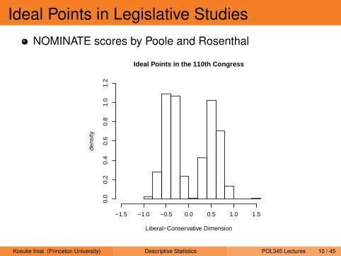
Ideal Points in Legislative Studies

NOMINATE scores by Poole and Rosenthal

Ideal Points in the 110th Congress

Liberal−Conservative Dimension

dens

ity

−1.5 −1.0 −0.5 0.0 0.5 1.0 1.5

0.0

0.2

0.4

0.6

0.8

1.0

1.2


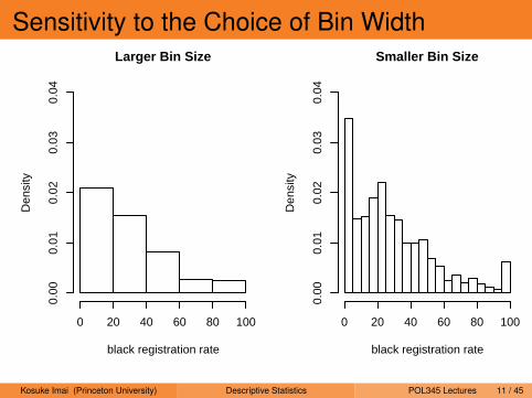
Sensitivity to the Choice of Bin WidthLarger Bin Size

black registration rate

Den

sity

0 20 40 60 80 100

0.00

0.01

0.02

0.03

0.04

Smaller Bin Size


Den

sity

0 20 40 60 80 1000.

000.

010.

020.

030.

04


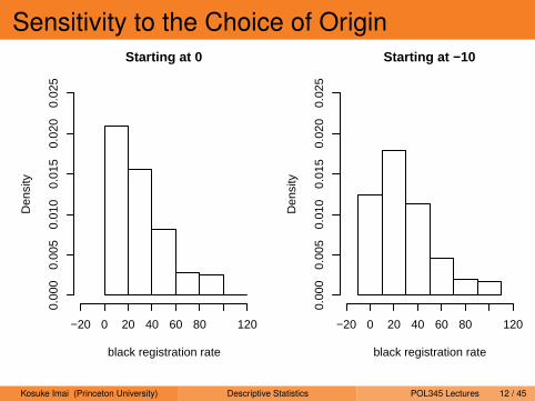
Sensitivity to the Choice of OriginStarting at 0


Den

sity

−20 0 20 40 60 80 120

0.00

00.

005

0.01

00.

015

0.02

00.

025

Starting at −10


Den

sity

−20 0 20 40 60 80 1200.

000

0.00

50.

010

0.01

50.

020

0.02

5


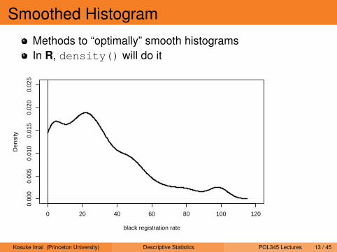
Smoothed Histogram

Methods to “optimally” smooth histogramsIn R, density() will do it

0 20 40 60 80 100 120

0.00

00.

005

0.01

00.

015

0.02

00.

025


Den

sity


Describing the Center of the Data

READING: FPP Chapter 4

(Sample) Mean or average:

X =1n

n∑i=1

Xi

(Sample) Median:

X =

{X( n+1

2 ) if n is odd12X( n

2)+ 1

2X( n2+1) if n is even

Mean is not necessarily medianMedian is more robust to outliers than meanExample: data = {0,1,2,3,100}, mean = 21.2, median = 2


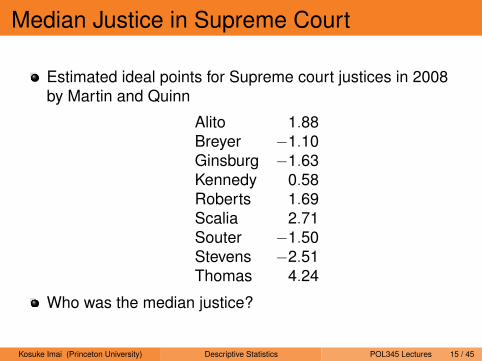
Median Justice in Supreme Court

Estimated ideal points for Supreme court justices in 2008by Martin and Quinn

Alito 1.88Breyer −1.10Ginsburg −1.63Kennedy 0.58Roberts 1.69Scalia 2.71Souter −1.50Stevens −2.51Thomas 4.24

Who was the median justice?


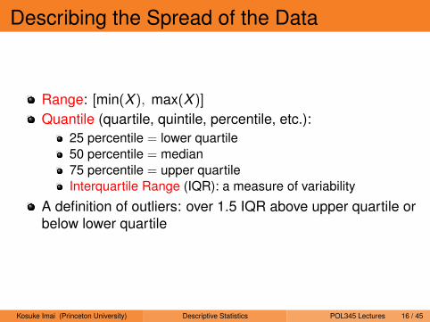
Describing the Spread of the Data

Range: [min(X ), max(X )]

Quantile (quartile, quintile, percentile, etc.):25 percentile = lower quartile50 percentile = median75 percentile = upper quartileInterquartile Range (IQR): a measure of variability

A definition of outliers: over 1.5 IQR above upper quartile orbelow lower quartile


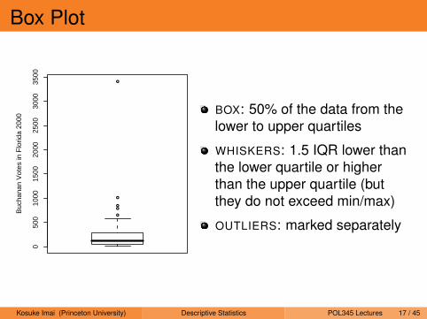
Box Plot

●

●

●

●

●

050

010

0015

0020

0025

0030

0035

00

Buc

hana

n V

otes

in F

lorid

a 20

00

BOX: 50% of the data from thelower to upper quartiles

WHISKERS: 1.5 IQR lower thanthe lower quartile or higherthan the upper quartile (butthey do not exceed min/max)

OUTLIERS: marked separately


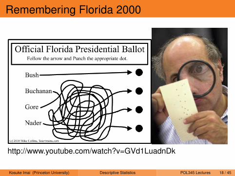
Remembering Florida 2000

http://www.youtube.com/watch?v=GVd1LuadnDk


http://www.youtube.com/watch?v=GVd1LuadnDk

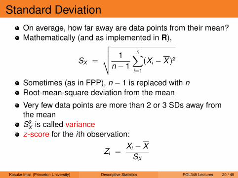
Standard DeviationOn average, how far away are data points from their mean?Mathematically (and as implemented in R),

SX =

√√√√ 1n − 1

n∑i=1

(Xi − X )2

Sometimes (as in FPP), n − 1 is replaced with nRoot-mean-square deviation from the mean

Very few data points are more than 2 or 3 SDs away fromthe meanS2

X is called variancez-score for the i th observation:

Zi =Xi − X

SX


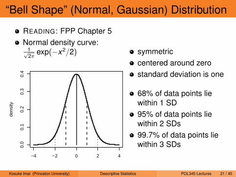
“Bell Shape” (Normal, Gaussian) Distribution

READING: FPP Chapter 5Normal density curve:

1√2π

exp(−x2/2)

−4 −2 0 2 4

0.0

0.1

0.2

0.3

0.4

dens

ity

symmetriccentered around zerostandard deviation is one

68% of data points liewithin 1 SD95% of data points liewithin 2 SDs99.7% of data points liewithin 3 SDs


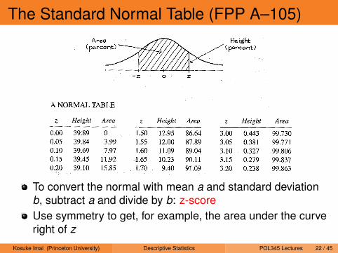
The Standard Normal Table (FPP A–105)

To convert the normal with mean a and standard deviationb, subtract a and divide by b: z-scoreUse symmetry to get, for example, the area under the curveright of z


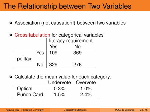
The Relationship between Two Variables

Association (not causation!) between two variables

Cross tabulation for categorical variablesliteracy requirementYes No

Yes 109 369polltax

No 329 276

Calculate the mean value for each category:Undervote Overvote

Optical 0.3% 1.0%Punch Card 1.5% 2.4%


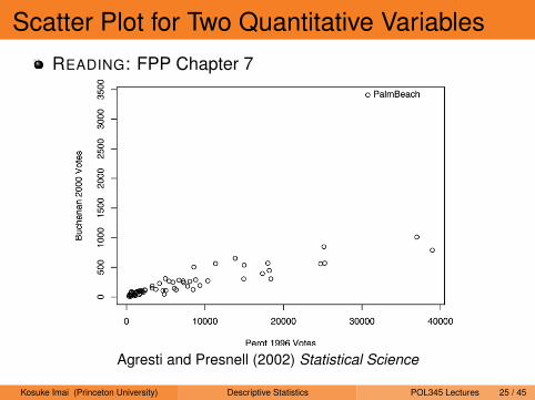
Scatter Plot for Two Quantitative VariablesREADING: FPP Chapter 7

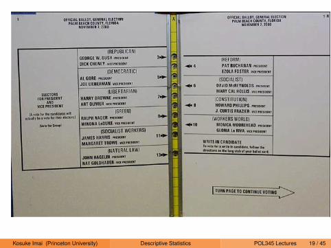
MISVOTES, UNDERVOTES AND OVERVOTES 437

FIG. 1. The Palm Beach county butterfly ballot.

the same: the Buchanan vote in Palm Beach county washighly anomalous.

Besides statistical modeling, other analyses sup-ported the contention that Buchanan may have re-ceived many votes intended for Gore. For instance,

Wand et al. (2001) noted that in Palm Beach county,Buchanan’s proportion of the vote on election-day bal-lots was four times his proportion on absentee (non-butterfly) ballots, yet the Buchanan proportion did notdiffer appreciably between election-day and absentee

FIG. 2. Total vote, by county, for Reform party candidates Buchanan in 2000 and Perot in 1996.Agresti and Presnell (2002) Statistical Science


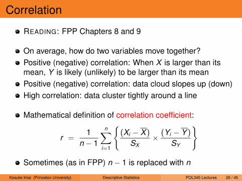
Correlation

READING: FPP Chapters 8 and 9

On average, how do two variables move together?Positive (negative) correlation: When X is larger than itsmean, Y is likely (unlikely) to be larger than its meanPositive (negative) correlation: data cloud slopes up (down)High correlation: data cluster tightly around a line

Mathematical definition of correlation coefficient:

r =1

n − 1

n∑i=1

{(Xi − X )

SX× (Yi − Y )

SY

}

Sometimes (as in FPP) n − 1 is replaced with n


Properties of Correlation Coefficient

Correlation is between −1 and 1

Order does not matter: cor(x,y) = cor(y,x)

Not affected by changes of scale:

cor(x,y) = cor(ax+ b,cy+ d)

for any numbers a, b, c, and d

Celsius vs. Fahrenheit; cm vs. inch; yen vs. dollar etc.

Correlation size is relative to standard deviationGiven the same correlation value, larger standarddeviations make data cloud look more spread around a line

Correlation only measures linear association


Correlation Doesn’t Always Imply Causation

The fact that two things tend to move together does notimply one causes the other

If correlation always implies causation...1 Having telephone increases the chance of breast cancer

death (correlation across 165 countries is 0.74)2 Population increase increases the chance of lung cancer

death (correlation is 0.92 in the US over the last 50 years)3 Gaining weight makes you vote for Bush or Voting for Bush

makes you fat (correlation between Bush’s voteshare andself-reported obesity rates in states is 0.40)

Predictive inference vs. Causal inferenceWhen does correlation imply causation?


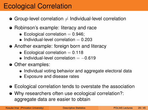
Ecological Correlation

Group-level correlation 6= Individual-level correlation

Robinson’s example: literacy and raceEcological correlation = 0.946;Individual-level correlation = 0.203

Another example: foreign born and literacyEcological correlation = 0.118Individual-level correlation = −0.619

Other examples:Individual voting behavior and aggregate electoral dataExposure and disease rates

Ecological correlation tends to overstate the associationWhy researchers often use ecological correlation?:aggregate data are easier to obtain


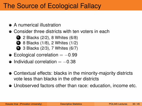
The Source of Ecological Fallacy

A numerical illustrationConsider three districts with ten voters in each

1 2 Blacks (2/2), 8 Whites (6/8)2 8 Blacks (1/8), 2 Whites (1/2)3 3 Blacks (2/3), 7 Whites (6/7)

Ecological correlation = −0.99Individual correlation = −0.38

Contextual effects: blacks in the minority-majority districtsvote less than blacks in the other districtsUnobserved factors other than race: education, income etc.


Linear Regression Model

READING: FPP Chapters 10 – 12

A model for a linear relationship between two variables

Yi = α + βXi + εi

X : Independent (explanatory) variableY : Dependent (outcome, response) variableε: error (disturbance) term

Given a value of X , the model predicts the average of YAbuse of regression: extrapolation, causal misinterpretation


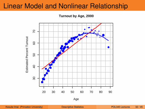
Linear Model and Nonlinear Relationship

20 30 40 50 60 70 80 90

3040

5060

70

Turnout by Age, 2000

Age

Est

imat

ed P

erce

nt T

urno

ut

●

●●

●

●

●

●●

●

●

●

●●●●●

●●●●

●●

●●●●●

●

●●●

●

●

●●●●●

●

●●

●

●●

●

●

●

●

●

●●

●

●●

●●

●

●

●

●

●

●

●

●


Galton (1886)’s Regression


The Regression Effect

Also called regression towards mean“When mid-parents are taller (shorter) than mediocrity, theirchildren tend to be shorter (taller) than they”Galton’s calculation illustrated:

(8 + 5 + 3)(1 + 2 + 3 + 5 + 8 + 9 + 9 + 8 + 5 + 3)

= 0.30

(13 + 10 + 7 + 3 + 1)(14 + 13 + 10 + 7 + 3 + 1 + 3 + 7 + 11 + 13)

= 0.41


Analysis of Regression Effect

If a student scores higher than average in the midterm, thenher final score is likely to be less than the midterm score.

A Regression Model: Yi = 15 + 0.8Xi + εi1 Yi : Final exam score for student i (percent)2 Xi : Midterm exam score for student i (percent)3 εi is normally distributed with mean = 0 and SD = 5

Two group of students: X1 = 60 and X2 = 80Which group of students is likely to do better in the final?

when compared with the other groupwhen compared with their own midterm score


Prediction and Prediction Error

Model parameters: (α, β)Estimates: (α, β)Predicted (fitted) value given Xi :

Yi = α + βXi

Prediction error (residual) = actual − predicted:

εi = Yi − Yi = Yi − (α + βXi)

r.m.s. of residuals =√

1− r 2SY

zero with perfect correlation r = ±1SY with zero correlation


Residuals and Residual PlotsMean of residuals: 1

n

∑ni=1 εi = 0

Does the regression model systematically overpredict orunderpredict for some observations?Heteroskedastic errors?

●● ●●

●

●

●

●●●

●●●●

●●

●●●●●●●●● ●● ●●

●●●● ●

●

●●●●●

●

●

●

●● ●●

●●

●

●

●

●●●

●●

●

●

●●●●●

● ●●

0 200 400 600 800 1200

−50

00

500

1500

2500

With Palm Beach

Fitted Values

Res

idua

ls

●● ●●●

●

●●

●●●

●●●

●●

●●●●●●●●●●●

●

● ●●●●

●

●

●●●● ●

●

● ●●●

●● ●●

● ●●●

●

●●

●

●●●●● ●● ●●

200 400 600 800 1000

−50

00

500

1500

2500

Without Palm Beach

Fitted Values

Res

idua

ls


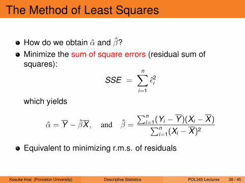
The Method of Least Squares

How do we obtain α and β?Minimize the sum of square errors (residual sum ofsquares):

SSE =n∑

i=1

ε2i

which yields

α = Y − βX , and β =

∑ni=1(Yi − Y )(Xi − X )∑n

i=1(Xi − X )2

Equivalent to minimizing r.m.s. of residuals


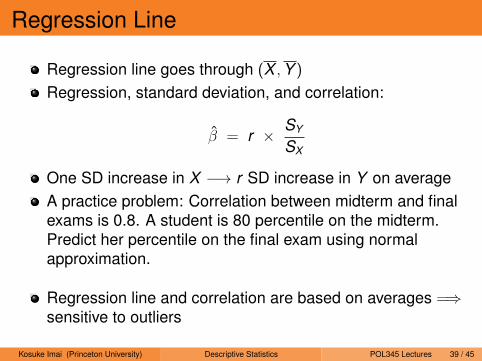
Regression Line

Regression line goes through (X ,Y )

Regression, standard deviation, and correlation:

β = r × SY

SX

One SD increase in X −→ r SD increase in Y on averageA practice problem: Correlation between midterm and finalexams is 0.8. A student is 80 percentile on the midterm.Predict her percentile on the final exam using normalapproximation.

Regression line and correlation are based on averages =⇒sensitive to outliers


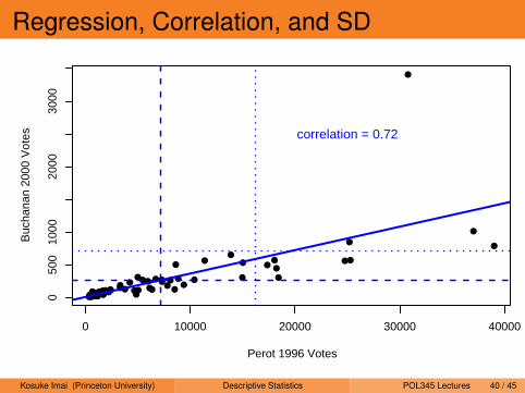
Regression, Correlation, and SD

●

●

●

●

●

●

●●

●●

●●●●

●

●

●●●●●●●●●

●●

●

● ●●●●

● ●●

●●●

●

●

●

●

●●

●

●

●

●

●

●

●

●

●

● ●●●

●●●●●

●

●●●

0 10000 20000 30000 40000

050

010

0020

0030

00

Perot 1996 Votes

Buc

hana

n 20

00 V

otes correlation = 0.72


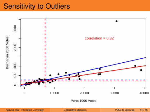
Sensitivity to Outliers

●

●

●

●

●

●

●●

●●

●●●●

●

●

●●●●●●●●●

●●

●

● ●●●●

● ●●

●●●

●

●

●

●

●●

●

●

●

●

●

●

●

●

●

● ●●●

●●●●●

●

●●●

0 10000 20000 30000 40000

050

010

0020

0030

00

Perot 1996 Votes

Buc

hana

n 20

00 V

otes correlation = 0.92


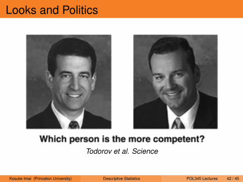
Looks and Politics

Todorov et al. Science


●

●

●●

●

●

●

●

●

●

●●

●

●

●

●

●●

●

●

●

● ● ●

●

●

●

●

●●

●

●

●●

●

●●

●

●

●

●●

●●

● ●

●

●

●

●

●●

●

●●

●

●

●

●●

●

●

●

●

●

●

●

●

●

●

●

●

●

●

●●

●

●●

●

●

●

●●

●

●

●

●

●●

●

●●

●●

0.0 0.2 0.4 0.6 0.8 1.0

−10

0−

500

5010

0

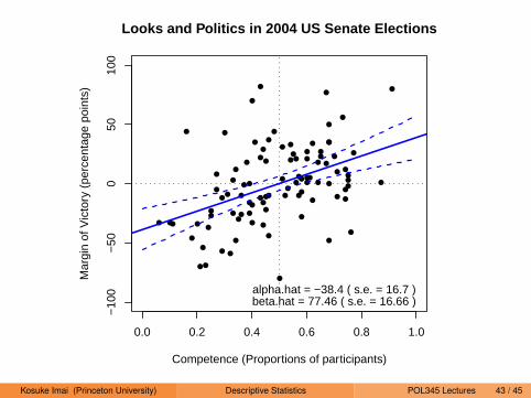
Looks and Politics in 2004 US Senate Elections

Competence (Proportions of participants)

Mar

gin

of V

icto

ry (

perc

enta

ge p

oint

s)

alpha.hat = −38.4 ( s.e. = 16.7 )beta.hat = 77.46 ( s.e. = 16.66 )


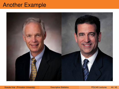
Another Example


Descriptive Statistics - Harvard University · Quantile(quartile, quintile, percentile, etc.): 25...

Documents

Transcript of Descriptive Statistics - Harvard University · Quantile(quartile, quintile, percentile, etc.): 25...