Derivative-Free Optimization: Theory and Practicelnv/talks/siopt-2008.pdf · Filters and...
233
Derivative-Free Optimization: Theory and Practice Charles Audet, ´ Ecole Polytechnique de Montr´ eal Lu´ ıs Nunes Vicente, Universidade de Coimbra Mini-tutorial – SIOPT 2008 – Boston May 2008
Transcript of Derivative-Free Optimization: Theory and Practicelnv/talks/siopt-2008.pdf · Filters and...

Derivative-Free Optimization:Theory and Practice
Charles Audet, Ecole Polytechnique de Montreal
Luıs Nunes Vicente, Universidade de Coimbra
Mini-tutorial – SIOPT 2008 – Boston
May 2008

Presentation Outline
1 Introduction
2 Unconstrained optimization
3 Optimization under general constraints
4 Surrogates, global DFO, software, and references

Presentation Outline
1 Introduction
2 Unconstrained optimizationDirectional direct search methodsSimplicial direct search and line-search methodsInterpolation-based trust-region methods
3 Optimization under general constraintsNonsmooth optimality conditionsMads and the extreme barrier for closed constraintsFilters and progressive barrier for open constraints
4 Surrogates, global DFO, software, and referencesThe surrogate management frameworkConstrained TR interpolation-based methodsTowards global DFO optimizationSoftware and references

Why derivative-free optimization
Some of the reasons to apply Derivative-Free Optimization are thefollowing:
Growing sophistication of computer hardware and mathematicalalgorithms and software (which opens new possibilities foroptimization).
Function evaluations costly and noisy (one cannot trust derivatives orapproximate them by finite differences).
Binary codes (source code not available or owned by a company) —making automatic differentiation impossible to apply.
Legacy codes (written in the past and not maintained by the originalauthors).
Lack of sophistication of the user (users need improvement but wantto use something simple).
Audet and Vicente (SIOPT 2008) Introduction 3/109

Examples of problems where derivatives are unavailable
Tuning of algorithmic parameters:
Most numerical codes depend on a number of critical parameters.
One way to automate the choice of the parameters (to find optimalvalues) is to solve:
minp∈Rnp
f(p) = CPU(p; solver) s.t. p ∈ P,
ormin
p∈Rnpf(p) = #iterations(p; solver) s.t. p ∈ P,
where np is the number of parameters to be tuned and P is of theform p ∈ Rnp : ` ≤ p ≤ u.
It is hard to calculate derivatives for such functions f (which are likelynoisy and non-differentiable).
Audet and Vicente (SIOPT 2008) Introduction 4/109

Examples of problems where derivatives are unavailable
Automatic error analysis:
A process in which the computer is used to analyze the accuracy orstability of a numerical computation.
How large can the growth factor for GE be for a pivoting strategy?Given n and a pivoting strategy, one maximizes the growth factor:
maxA∈Rn×n
f(A) =maxi,j,k |a
(k)ij |
maxi,j |aij |.
A starting point could be A0 = In.
When no pivoting is chosen, f is defined and continuous at all pointswhere GE does not break down (possibly non-differentiability).
For partial pivoting, the function f is defined everywhere (because GEcannot break down) but it can be discontinuous when a tie occurs.
Audet and Vicente (SIOPT 2008) Introduction 5/109

Examples of problems where derivatives are unavailable
Engineering design:
A case study in DFO is the helicopter rotor blade design problem:
The goal is to find the structural design of the rotor blades to minimizethe vibration transmitted to the hub. The variables are the mass,center of gravity, and stiffness of each segment of the rotor blade.
The simulation code is multidisciplinary, including dynamic structures,aerodynamics, and wake modeling and control.
The problem includes upper and lower bounds on the variables, andsome linear constraints have been considered such as an upper boundon the sum of masses.
Each function evaluation requires simulation and can take fromminutes to days of CPU time.
Other examples are wing platform design, aeroacoustic shape design,and hydrodynamic design.
Audet and Vicente (SIOPT 2008) Introduction 6/109

Examples of problems where derivatives are unavailable
Other known applications:
Circuit design (tuning parameters of relatively small circuits).
Molecular geometry optimization (minimization of the potentialenergy of clusters).
Groundwater community problems.
Medical image registration.
Dynamic pricing.
Audet and Vicente (SIOPT 2008) Introduction 7/109

Limitations of derivative-free optimization
iteration ‖xk − x∗‖0 1.8284e+0001 5.9099e-0012 1.0976e-0013 5.4283e-0034 1.4654e-0055 1.0737e-0106 1.1102e-016
Newton methods converge quadratically (locally) but require first andsecond order derivatives (gradient and Hessian).
Audet and Vicente (SIOPT 2008) Introduction 8/109

Limitations of derivative-free optimization
iteration ‖xk − x∗‖0 3.0000e+0001 2.0002e+0002 6.4656e-001...
...6 1.4633e-0017 4.0389e-0028 6.7861e-0039 6.5550e-00410 1.4943e-00511 8.3747e-00812 8.8528e-010
Quasi Newton (secant) methods converge superlinearly (locally) butrequire first order derivatives (gradient).
Audet and Vicente (SIOPT 2008) Introduction 9/109

Limitations of derivative-free optimization
In DFO convergence/stopping is typically slow (per function evaluation):
Audet and Vicente (SIOPT 2008) Introduction 10/109

Pitfalls
The objective function might not be continuous or even well defined:
Audet and Vicente (SIOPT 2008) Introduction 11/109

Pitfalls
The objective function might not be continuous or even well defined:
Audet and Vicente (SIOPT 2008) Introduction 12/109

What can we solve
With the current state-of-the-art DFO methods one can expect tosuccessfully address problems where:
The evaluation of the function is expensive and/or computed withnoise (and for which accurate finite-difference derivative estimation isprohibitive and automatic differentiation is ruled out).
The number of variables does not exceed, say, a hundred (in serialcomputation).
The functions are not excessively non-smooth.
Rapid asymptotic convergence is not of primary importance.
Only a few digits of accuracy are required.
Audet and Vicente (SIOPT 2008) Introduction 13/109

What can we solve
In addition we can expect to solve problems:
With hundreds of variables using a parallel environment or exploitingproblem information.
With a few integer or categorical variables.
With a moderate level of multimodality:
It is hard to minimize non-convex functions without derivatives.
However, it is generally accepted that derivative-free optimizationmethods have the ability to find ‘good’ local optima.
DFO methods have a tendency to: (i) go to generally low regions inthe early iterations; (ii) ‘smooth’ the function in later iterations.
Audet and Vicente (SIOPT 2008) Introduction 14/109

Classes of algorithms (globally convergent)
Over-simplifying, all globally convergent DFO algorithms must:
Guarantee some form of descent away from stationarity.
Guarantee some control of the geometry of the sample sets where theobjective function is evaluated.
Imply convergence of step size parameters to zero, indicating globalconvergence to a stationary point.
By global convergence we mean convergence to some form of stationarityfrom arbitrary starting points.
Audet and Vicente (SIOPT 2008) Introduction 15/109
Classes of algorithms (globally convergent)
(Directional) Direct Search:
Achieve descent by using positive bases or positive spanning sets andmoving in the directions of the best points (in patterns or meshes).
Examples are coordinate search, pattern search, generalized patternsearch (GPS), generating set search (GSS), mesh adaptive directsearch (MADS).
Audet and Vicente (SIOPT 2008) Introduction 16/109
Classes of algorithms (globally convergent)
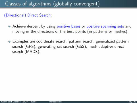
(Simplicial) Direct Search:
Ensure descent from simplex operations like reflections, by moving inthe direction away from the point with the worst function value.
Examples are the Nelder-Mead method and several modifications toNelder-Mead.
Audet and Vicente (SIOPT 2008) Introduction 17/109

Classes of algorithms (globally convergent)
Line-Search Methods:
Aim to get descent along negative simplex gradients (which areintimately related to polynomial models).
Examples are the implicit filtering method.
Audet and Vicente (SIOPT 2008) Introduction 18/109

Classes of algorithms (globally convergent)
Trust-Region Methods:
Minimize trust-region subproblems defined by fully-linear orfully-quadratic models (typically built from interpolation orregression).
Examples are methods based on polynomial models or radial basisfunctions models.
Audet and Vicente (SIOPT 2008) Introduction 19/109

Presentation outline
1 Introduction
2 Unconstrained optimizationDirectional direct search methodsSimplicial direct search and line-search methodsInterpolation-based trust-region methods
3 Optimization under general constraints
4 Surrogates, global DFO, software, and references

Direct search methods
Use the function values directly.
Do not require derivatives.
Do not attempt to estimate derivatives.
Mads is guaranteed to produce solutions that satisfy hierarchicaloptimality conditions depending on local smoothness of the functions.
Examples: DiRect, Mads, Nelder-Mead, Pattern Search.
Audet and Vicente (SIOPT 2008) Unconstrained optimization 21/109

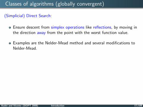
Coordinate search (ancestor of pattern search).
Consider the unconstrained problem
minx∈Rn
f(x)
where f : Rn → R ∪ ∞.
Initialization:x0 : initial point in Rn such that f(x0) <∞∆0 > 0 : initial mesh size.
Poll step: for k = 0, 1, . . .If f(t) < f(xk) for some t ∈ Pk := xk ±∆kei : i ∈ N,
then set xk+1 = tand ∆k+1 = ∆k;
otherwise xk is a local minimum with respect to Pk,set xk+1 = xk
and ∆k+1 = ∆k2 .
Audet and Vicente (SIOPT 2008) Unconstrained optimization 22/109

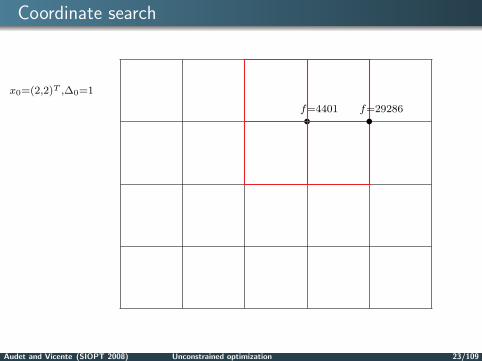
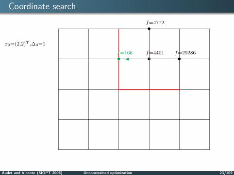
Coordinate search
x0=(2,2)T ,∆0=1
•f=4401
•f=29286
•f=4772
•f=166
Audet and Vicente (SIOPT 2008) Unconstrained optimization 23/109

Coordinate search
x0=(2,2)T ,∆0=1
•f=4401
•f=29286
•f=4772
•f=166
Audet and Vicente (SIOPT 2008) Unconstrained optimization 23/109

Coordinate search
x0=(2,2)T ,∆0=1
•f=4401
•f=29286
•f=4772
•f=166
Audet and Vicente (SIOPT 2008) Unconstrained optimization 23/109
Coordinate search
x0=(2,2)T ,∆0=1
•f=4401
•f=29286
•f=4772
•f=166
Audet and Vicente (SIOPT 2008) Unconstrained optimization 23/109

Coordinate search
x0=(2,2)T ,∆0=1
•f=4401
•f=29286
•f=4772
•f=166
Audet and Vicente (SIOPT 2008) Unconstrained optimization 23/109

Coordinate search
x0=(2,2)T ,∆0=1
•f=4401
•f=29286
•f=4772
•f=166
Audet and Vicente (SIOPT 2008) Unconstrained optimization 23/109
Coordinate search
x0=(2,2)T ,∆0=1
•f=4401
•f=29286
•f=4772
•f=166
Audet and Vicente (SIOPT 2008) Unconstrained optimization 23/109

Coordinate search
x1=(1,2)T ,∆1=1
•f=166
•f=81
Audet and Vicente (SIOPT 2008) Unconstrained optimization 24/109

Coordinate search
x1=(1,2)T ,∆1=1
•f=166
•f=81
Audet and Vicente (SIOPT 2008) Unconstrained optimization 24/109

Coordinate search
x1=(1,2)T ,∆1=1
•f=166
•f=81
Audet and Vicente (SIOPT 2008) Unconstrained optimization 24/109

Coordinate search
x2=(2,2)T ,∆2=1
•f=81
•f=2646
•f=166
•f=152
•f=36
Audet and Vicente (SIOPT 2008) Unconstrained optimization 25/109

Coordinate search
x2=(2,2)T ,∆2=1
•f=81
•f=2646
•f=166
•f=152
•f=36
Audet and Vicente (SIOPT 2008) Unconstrained optimization 25/109

Coordinate search
x2=(2,2)T ,∆2=1
•f=81
•f=2646
•f=166
•f=152
•f=36
Audet and Vicente (SIOPT 2008) Unconstrained optimization 25/109

Coordinate search
x2=(2,2)T ,∆2=1
•f=81
•f=2646
•f=166
•f=152
•f=36
Audet and Vicente (SIOPT 2008) Unconstrained optimization 25/109

Coordinate search
x2=(2,2)T ,∆2=1
•f=81
•f=2646
•f=166
•f=152
•f=36
Audet and Vicente (SIOPT 2008) Unconstrained optimization 25/109

Coordinate search
x3=(0,1)T ,∆3=1
•f=36
•f=17
Audet and Vicente (SIOPT 2008) Unconstrained optimization 26/109

Coordinate search
x3=(0,1)T ,∆3=1
•f=36
•f=17
Audet and Vicente (SIOPT 2008) Unconstrained optimization 26/109

Coordinate search
x4=(0,0)T ,∆4=1
•f=17
•f=24
•f=2402
•f=82
•f=36
Audet and Vicente (SIOPT 2008) Unconstrained optimization 27/109

Coordinate search
x4=(0,0)T ,∆4=1
•f=17
•f=24
•f=2402
•f=82
•f=36
Audet and Vicente (SIOPT 2008) Unconstrained optimization 27/109

Coordinate search
x5=(0,0)T ,∆5= 12
•f=17
•f=18
•f=40
•f=2
Audet and Vicente (SIOPT 2008) Unconstrained optimization 28/109

Coordinate search
x5=(0,0)T ,∆5= 12
•f=17
•f=18
•f=40
•f=2
Audet and Vicente (SIOPT 2008) Unconstrained optimization 28/109

Coordinate search
x5=(0,0)T ,∆5= 12
•f=17
•f=18
•f=40
•f=2
Audet and Vicente (SIOPT 2008) Unconstrained optimization 28/109

Generalized pattern search – Torczon 1996
Initialization:x0 : initial point in Rn such that f(x0) <∞∆0 > 0 : initial mesh size.D : finite positive spanning set of directions.
Audet and Vicente (SIOPT 2008) Unconstrained optimization 29/109

Generalized pattern search – Torczon 1996
Initialization:x0 : initial point in Rn such that f(x0) <∞∆0 > 0 : initial mesh size.D : finite positive spanning set of directions.
Definition
D = d1, d2, . . . , dp is a positive spanning set ifp∑
i=1
αidi : αi ≥ 0, i = 1, 2, . . . p
= Rn.
Remark : p ≥ n + 1.
Definition (Davis)
D = d1, d2, . . . , dp is a positive basis is it is a positive spanning set andno proper subset of D is a positive spanning set.Remark : n + 1 ≤ p ≤ 2n.
Audet and Vicente (SIOPT 2008) Unconstrained optimization 29/109

Generalized pattern search – Torczon 1996
Initialization:x0 : initial point in Rn such that f(x0) <∞∆0 > 0 : initial mesh size.D : finite positive spanning set of directions.For k = 0, 1, . . .
Search step: Evaluate f at a finite number of mesh points.Poll step: If the search failed, evaluate f at the poll pointsxk + ∆kd : d ∈ Dk where Dk ⊂ D is a positive spanning set.Parameter update:Set ∆k+1 < ∆k if no new incumbent was found,otherwise set ∆k+1 ≥ ∆k, and call xk+1 the new incumbent.
Audet and Vicente (SIOPT 2008) Unconstrained optimization 29/109

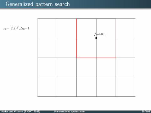
Generalized pattern search
x0=(2,2)T ,∆0=1
•f=4401
@@
@@
@
•f=4772
•f=101
Audet and Vicente (SIOPT 2008) Unconstrained optimization 30/109
Generalized pattern search
x0=(2,2)T ,∆0=1
•f=4401
@@
@@
@
•f=4772
•f=101
Audet and Vicente (SIOPT 2008) Unconstrained optimization 30/109

Generalized pattern search
x0=(2,2)T ,∆0=1
•f=4401
@@
@@
@
•f=4772
•f=101
Audet and Vicente (SIOPT 2008) Unconstrained optimization 30/109

Generalized pattern search
x0=(2,2)T ,∆0=1
•f=4401
@@
@@
@
•f=4772
•f=101
Audet and Vicente (SIOPT 2008) Unconstrained optimization 30/109

Generalized pattern search
x0=(2,2)T ,∆0=1
•f=4401
@@
@@
@
•f=4772
•f=101
Audet and Vicente (SIOPT 2008) Unconstrained optimization 30/109
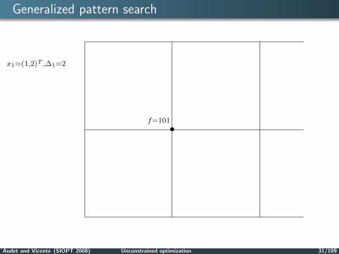
Generalized pattern search
x1=(1,2)T ,∆1=2
•f=101
•f=150
•f=2341
•f=967
Audet and Vicente (SIOPT 2008) Unconstrained optimization 31/109

Generalized pattern search
x1=(1,2)T ,∆1=2
•f=101
•f=150
•f=2341
•f=967
Audet and Vicente (SIOPT 2008) Unconstrained optimization 31/109

Generalized pattern search
x1=(1,2)T ,∆1=2
•f=101
•f=150
•f=2341
•f=967
Audet and Vicente (SIOPT 2008) Unconstrained optimization 31/109

Generalized pattern search
x2=(2,2)T ,∆2=1
•f=101
•A search trial point. Ex: built using a simplex gradient
Audet and Vicente (SIOPT 2008) Unconstrained optimization 32/109

Generalized pattern search
x2=(2,2)T ,∆2=1
•f=101
•A search trial point. Ex: built using a simplex gradient
Audet and Vicente (SIOPT 2008) Unconstrained optimization 32/109

Convergence analysis
If all iterates belong to a bounded set, then lim infk ∆k = 0.
Corollary
There is a convergent subsequence of iterates xk → x of mesh localoptimizers, on meshes that get infinitely fine.
Audet and Vicente (SIOPT 2008) Unconstrained optimization 33/109

Convergence analysis
If all iterates belong to a bounded set, then lim infk ∆k = 0.
Corollary
There is a convergent subsequence of iterates xk → x of mesh localoptimizers, on meshes that get infinitely fine.
GPS methods are directional. The analysis is tied to the fixed set ofdirections D: f(xk) ≤ f(xk + ∆kd) for every d ∈ Dk ⊆ D.
Theorem
If f is Lipschitz near x, then for every direction d ∈ D used infinitely often,
f(x; d) := lim supy→x,t→0
f(y + td)− f(y)t
≥ lim supk
f(xk + ∆kd)− f(xk)∆k
≥ 0.
Audet and Vicente (SIOPT 2008) Unconstrained optimization 33/109

Convergence analysis
If all iterates belong to a bounded set, then lim infk ∆k = 0.
Corollary
There is a convergent subsequence of iterates xk → x of mesh localoptimizers, on meshes that get infinitely fine.
GPS methods are directional. The analysis is tied to the fixed set ofdirections D: f(xk) ≤ f(xk + ∆kd) for every d ∈ Dk ⊆ D.
Corollary
If f is regular near x, then for every direction d ∈ D used infinitely often,
f ′(x; d) := limt→0
f(x + td)− f(x)t
≥ 0.
Audet and Vicente (SIOPT 2008) Unconstrained optimization 33/109

Convergence analysis
If all iterates belong to a bounded set, then lim infk ∆k = 0.
Corollary
There is a convergent subsequence of iterates xk → x of mesh localoptimizers, on meshes that get infinitely fine.
GPS methods are directional. The analysis is tied to the fixed set ofdirections D: f(xk) ≤ f(xk + ∆kd) for every d ∈ Dk ⊆ D.
Corollary
If f is strictly differentiable near x, then
∇f(x) = 0.
Audet and Vicente (SIOPT 2008) Unconstrained optimization 33/109

Related methods
The GPS iterates at each iteration are confined to reside on the mesh.
The mesh gets finer and finer, but still, some users want to evaluatethe functions at non-mesh points.
Frame-based methods, and Generalized Set Search methods removethis restriction to the mesh. The trade-off is that they require aminimal decrease on the objective to accept new solutions.
gps: trial points on the mesh
rxk
.
..............
..................................................................
.................................
................................... .......... ............. ............... .................. ..................... ....................... .......................... ............................. ..........................................................................................
gss: trial points away from xk
rxk
Audet and Vicente (SIOPT 2008) Unconstrained optimization 34/109

Related methods
The GPS iterates at each iteration are confined to reside on the mesh.
The mesh gets finer and finer, but still, some users want to evaluatethe functions at non-mesh points.
Frame-based methods, and Generalized Set Search methods removethis restriction to the mesh. The trade-off is that they require aminimal decrease on the objective to accept new solutions.
direct partitions the space of variables into hyperrectangles, anditeratively refines the most promising ones.
Figure taken from Finkel and Kelley CRSC-TR04-30.
Audet and Vicente (SIOPT 2008) Unconstrained optimization 34/109

Presentation outline
1 Introduction
2 Unconstrained optimizationDirectional direct search methodsSimplicial direct search and line-search methodsInterpolation-based trust-region methods
3 Optimization under general constraintsNonsmooth optimality conditionsMads and the extreme barrier for closed constraintsFilters and progressive barrier for open constraints
4 Surrogates, global DFO, software, and referencesThe surrogate management frameworkConstrained TR interpolation-based methodsTowards global DFO optimizationSoftware and references
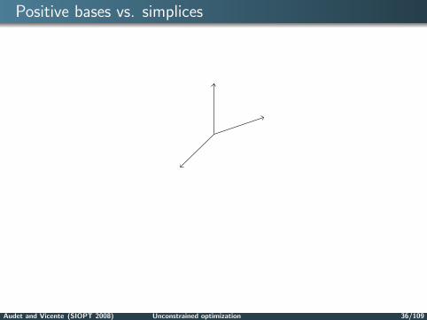
Positive bases vs. simplices
Audet and Vicente (SIOPT 2008) Unconstrained optimization 36/109

Positive bases vs. simplices
Audet and Vicente (SIOPT 2008) Unconstrained optimization 36/109

Positive bases vs. simplices
The 3 = n + 1 points form an affinely independent set.
A set of m + 1 points Y = y0, y1, . . . , ym is said to be affinely independent
if its affine hull aff(y0, y1, . . . , ym) has dimension m.
Audet and Vicente (SIOPT 2008) Unconstrained optimization 36/109

Positive bases vs. simplices
Their convex hull is a simplex of dimension n = 2.
Given an affinely independent set of points Y = y0, y1, . . . , ym,its convex hull is called a simplex of dimension m.
Audet and Vicente (SIOPT 2008) Unconstrained optimization 36/109

Positive bases vs. simplices
Its reflection produces a (maximal) positive basis.
Audet and Vicente (SIOPT 2008) Unconstrained optimization 36/109

Simplices
The volume of a simplex of vertices Y = y0, y1, . . . , yn is defined by
vol(Y ) =|det(S(Y ))|
n!
whereS(Y ) =
[y1 − y0 · · · yn − y0
].
Note that vol(Y ) > 0 (since the vertices are affinely independent).
A measure of geometry for simplices is the normalized volume:
von(Y ) = vol(
1diam(Y )
Y
).
Audet and Vicente (SIOPT 2008) Unconstrained optimization 37/109

Simplicial Direct-Search Methods
The Nelder-Mead method:
Considers a simplex at each iteration, trying to replace the worstvertex by a new one.
For that it performs one of the following simplex operations:reflexion, expansion, outside contraction, inside contraction.
−→ Costs 1 or 2 function evaluations (per iteration).
If they all the above fail the simplex is shrunk.
−→ Additional n function evaluations (per iteration).
Audet and Vicente (SIOPT 2008) Unconstrained optimization 38/109

Nelder Mead simplex operations (reflections, expansions, outsidecontractions, inside contractions)
yr yeyic yocy2
y1
y0
yc
yc is the centroid of the face opposed to the worse vertex y2.
Audet and Vicente (SIOPT 2008) Unconstrained optimization 39/109

Nelder Mead simplex operations (shrinks)
y2
y1
y0
Audet and Vicente (SIOPT 2008) Unconstrained optimization 40/109

McKinnon counter-example:The Nelder-Mead method:
Attempts to capture the curvature of the function.
Is globally convergent when n = 1.
Can fail for n > 1 (e.g. due to repeated inside contractions).
Audet and Vicente (SIOPT 2008) Unconstrained optimization 41/109

McKinnon counter-example
Audet and Vicente (SIOPT 2008) Unconstrained optimization 42/109

Nelder-Mead on McKinnon example (two different starting simplices)
Audet and Vicente (SIOPT 2008) Unconstrained optimization 43/109

Modified Nelder-Mead methodsFor Nelder-Mead to globally converge one must:
Control the internal angles (normalized volume) in all simplexoperations but shrinks.
CAUTION (very counterintuitive): Isometric reflections only preserveinternal angles when n = 2 or the simplices are equilateral.
−→ Need for a back-up polling.
Impose sufficient decrease instead of simple decrease for acceptingnew iterates:
f(new point) ≤ f(previous point)− o(simplex diameter).
Audet and Vicente (SIOPT 2008) Unconstrained optimization 44/109

Modified Nelder-Mead methods
Let Yk be the sequence of simplices generated.Let f be bounded from below and uniformly continuous in Rn.
Theorem (Step size going to zero)
The diameters of the simplices converge to zero:
limk−→+∞
diam(Yk) = 0.
Theorem (Global convergence)
If f is continuously differentiable in Rn and Yk lies in a compact set then
Yk has at least one stationary limit point x∗.
Audet and Vicente (SIOPT 2008) Unconstrained optimization 45/109

Simplex gradients
It is possible to build a simplex gradient:
y0
y1
y2
∇sf(y0) =[
y1 − y0 y2 − y0]−> [
f(y1)− f(y0)f(y2)− f(y0)
].
Audet and Vicente (SIOPT 2008) Unconstrained optimization 46/109

Simplex gradients
It is possible to build a simplex gradient:
y0
y1
y2
∇sf(y0) = S−>δ(f).
Audet and Vicente (SIOPT 2008) Unconstrained optimization 46/109

Simplex gradients
Simple Fact (What is a simplex gradient)
The simplex gradient (based on n + 1 affinely independent points) is thegradient of the corresponding linear interpolation model:
f(y0) + 〈∇sf(y0), yi − y0〉 = f(y0) +(S−>δ(f)
)> (Sei)
= f(y0) + δ(f)i
= f(yi).
−→ Simplex derivatives are the derivatives of the polynomial models.
Audet and Vicente (SIOPT 2008) Unconstrained optimization 47/109
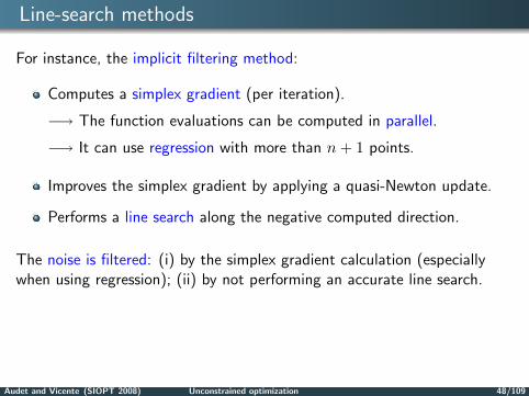
Line-search methods
For instance, the implicit filtering method:
Computes a simplex gradient (per iteration).
−→ The function evaluations can be computed in parallel.
−→ It can use regression with more than n + 1 points.
Improves the simplex gradient by applying a quasi-Newton update.
Performs a line search along the negative computed direction.
The noise is filtered: (i) by the simplex gradient calculation (especiallywhen using regression); (ii) by not performing an accurate line search.
Audet and Vicente (SIOPT 2008) Unconstrained optimization 48/109

Presentation outline
1 Introduction
2 Unconstrained optimizationDirectional direct search methodsSimplicial direct search and line-search methodsInterpolation-based trust-region methods
3 Optimization under general constraintsNonsmooth optimality conditionsMads and the extreme barrier for closed constraintsFilters and progressive barrier for open constraints
4 Surrogates, global DFO, software, and referencesThe surrogate management frameworkConstrained TR interpolation-based methodsTowards global DFO optimizationSoftware and references

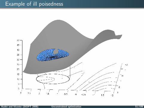
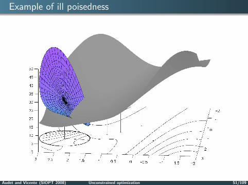
Trust-Region Methods for DFO (basics)
Trust-region methods for DFO typically:
attempt to form quadratic models (by interpolation/regression andusing polynomials or radial basis functions)
m(∆x) = f(xk) + 〈gk,∆x〉+ 1/2〈∆x,Hk∆x〉
based on well-poised sample sets.
−→ Well poisedness ensures fully-linear or fully quadratic models.
Calculate a step ∆xk by solving
min∆x∈B(xk;∆k)
m(∆x).
Audet and Vicente (SIOPT 2008) Unconstrained optimization 50/109

Example of ill poisedness
Audet and Vicente (SIOPT 2008) Unconstrained optimization 51/109

Example of ill poisedness
Audet and Vicente (SIOPT 2008) Unconstrained optimization 51/109
Example of ill poisedness
Audet and Vicente (SIOPT 2008) Unconstrained optimization 51/109
Example of ill poisedness
Audet and Vicente (SIOPT 2008) Unconstrained optimization 51/109

Fully-linear models
Given a point x and a trust-region radius ∆, a model m(y) around x iscalled fully linear if
It is continuous differentiable with Lipschitz continuous firstderivatives.
The following error bounds hold:
‖∇f(y)−∇m(y)‖ ≤ κeg ∆ ∀y ∈ B(x;∆)
and|f(y)−m(y)| ≤ κef ∆2 ∀y ∈ B(x;∆).
For a class of fully-linear models, the (unknown) constants κef , κeg > 0must be independent of x and ∆.
Audet and Vicente (SIOPT 2008) Unconstrained optimization 52/109

Fully-linear models
For a class of fully-linear models, one must also guarantee that:
There exists a model-improvement algorithm, that in a finite,uniformly bounded (with respect to x and ∆) number of steps can:
— certificate that a given model is fully linear on B(x;∆),
— or (if the above fails), find a model that is fully linear on B(x;∆).
Audet and Vicente (SIOPT 2008) Unconstrained optimization 53/109

Fully-quadratic models
Given a point x and a trust-region radius ∆, a model m(y) around x iscalled fully quadratic if
It is twice continuous differentiable with Lipschitz continuous secondderivatives.
The following error bounds hold (...):
‖∇2f(y)−∇2m(y)‖ ≤ κeh ∆ ∀y ∈ B(x;∆)
‖∇f(y)−∇m(y)‖ ≤ κeg ∆2 ∀y ∈ B(x;∆)
and|f(y)−m(y)| ≤ κef ∆3 ∀y ∈ B(x;∆).
Audet and Vicente (SIOPT 2008) Unconstrained optimization 54/109
TR methods for DFO (basics)
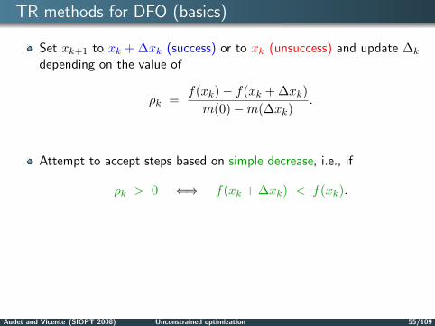
Set xk+1 to xk + ∆xk (success) or to xk (unsuccess) and update ∆k
depending on the value of
ρk =f(xk)− f(xk + ∆xk)
m(0)−m(∆xk).
Attempt to accept steps based on simple decrease, i.e., if
ρk > 0 ⇐⇒ f(xk + ∆xk) < f(xk).
Audet and Vicente (SIOPT 2008) Unconstrained optimization 55/109

TR methods for DFO (main features)
Reduce ∆k only if ρk is small and the model is FL/FQ.
Accept new iterates based on simple decrease (ρk > 0) as long as themodel is FL/FQ
Allow for model-improving iterations (when ρk is not large enoughand the model is not certifiably FL/FQ).
−→ Do not reduce ∆k.
Incorporate a criticality step (1st or 2nd order) when the ‘stationarity’of the model is small.
−→ Internal cycle of reductions of ∆k.
Audet and Vicente (SIOPT 2008) Unconstrained optimization 56/109
TR methods for DFO (global convergence)
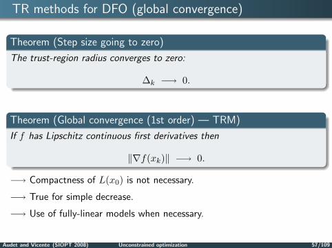
Theorem (Step size going to zero)
The trust-region radius converges to zero:
∆k −→ 0.
Theorem (Global convergence (1st order) — TRM)
If f has Lipschitz continuous first derivatives then
‖∇f(xk)‖ −→ 0.
−→ Compactness of L(x0) is not necessary.
−→ True for simple decrease.
−→ Use of fully-linear models when necessary.
Audet and Vicente (SIOPT 2008) Unconstrained optimization 57/109

TR methods for DFO (global convergence)
Theorem (Global convergence (2nd order) — TRM)
If f has Lipschitz continuous second derivatives then
max‖∇f(xk)‖,−λmin[∇2f(xk)]
−→ 0.
−→ Compactness of L(x0) is not necessary.
−→ True for simple decrease.
−→ Use of fully-quadratic models when necessary.
Audet and Vicente (SIOPT 2008) Unconstrained optimization 58/109

Polynomial models
Given a sample set Y = y0, y1, . . . , yp and a polynomial basis φ, oneconsiders a system of linear equations:
M(φ, Y )α = f(Y ),
where
M(φ, Y ) =
φ0(y0) φ1(y0) · · · φp(y0)φ0(y1) φ1(y1) · · · φp(y1)
......
......
φ0(yp) φ1(yp) · · · φp(yp)
f(Y ) =
f(y0)f(y1)
...f(yp)
.
Example: φ = 1, x1, x2, x21/2, x2
2/2, x1x2.
Audet and Vicente (SIOPT 2008) Unconstrained optimization 59/109

Polynomial models
The systemM(φ, Y )α = f(Y )
can be
Determined when (# points) = (# basis components).
Overdetermined when (# points) > (# basis components).
−→ least-squares regression solution.
Undetermined when (# points) < (# basis components).
−→ minimum-norm solution
−→ minimum Frobenius norm solution
Audet and Vicente (SIOPT 2008) Unconstrained optimization 60/109

Error bounds for polynomial models
Given an interpolation set Y , the error bounds (# points ≥ n + 1) are ofthe form
‖∇f(y)−∇m(y)‖ ≤ [C(n)C(f)C(Y )] ∆ ∀y ∈ B(x;∆)
where
C(n) is a small constant depending on n.
C(f) measures the smoothness of f (in this case the Lipschitzconstant of ∇f).
C(Y ) is related to the geometry of Y .
Audet and Vicente (SIOPT 2008) Unconstrained optimization 61/109
Geometry constants
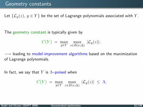
Let Ly(z), y ∈ Y be the set of Lagrange polynomials associated with Y .
The geometry constant is typically given by
C(Y ) = maxy∈Y
maxz∈B(x;∆)
|Ly(z)| .
−→ leading to model-improvement algorithms based on the maximizationof Lagrange polynomials.
In fact, we say that Y is Λ–poised when
C(Y ) = maxy∈Y
maxz∈B(x;∆)
|Ly(z)| ≤ Λ.
Audet and Vicente (SIOPT 2008) Unconstrained optimization 62/109

Model improvement (Lagrange polynomials)
Choose Λ > 1. Let Y be a poised set.
Each iteration of a model-improvement algorithm consists of:
EstimateC = max
y∈Ymaxz∈B|Ly(z)|.
If C > Λ then let yout correspond to the polynomial where themaximum was attained. Let
yin ∈ argmaxz∈B |Lyout(z)|.
Update Y (and the Lagrange polynomials):
Y ← Y ∪ yin \ yout.
Otherwise (i.e., C ≤ Λ), Y is Λ–poised and stop.
Audet and Vicente (SIOPT 2008) Unconstrained optimization 63/109

Model improvement (Lagrange polynomials)
Theorem
For any given Λ > 1 and a closed ball B, the previous model-improvementalgorithm terminates with a Λ–poised set Y after at most N = N(Λ)iterations.
Audet and Vicente (SIOPT 2008) Unconstrained optimization 64/109

Example (model improvement based on LP)
C = 5324
Audet and Vicente (SIOPT 2008) Unconstrained optimization 65/109

Example (model improvement based on LP)
C = 36.88
Audet and Vicente (SIOPT 2008) Unconstrained optimization 65/109

Example (model improvement based on LP)
C = 15.66
Audet and Vicente (SIOPT 2008) Unconstrained optimization 65/109
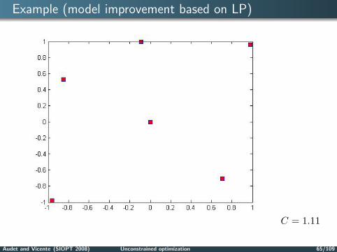
Example (model improvement based on LP)
C = 1.11
Audet and Vicente (SIOPT 2008) Unconstrained optimization 65/109

Example (model improvement based on LP)
C = 1.01
Audet and Vicente (SIOPT 2008) Unconstrained optimization 65/109

Example (model improvement based on LP)
C = 1.001
Audet and Vicente (SIOPT 2008) Unconstrained optimization 65/109

Geometry constants
The geometry constant can also be given by
C(Y ) = cond(scaled interpolation matrix M)
−→ leading to model-improvement algorithms based on pivotalfactorizations (LU/QR or Newton polynomials).
These algorithms yield:
‖M−1‖ ≤ C(n)εgrowth
ξ
where
εgrowth is the growth factor of the factorization.
ξ > 0 is a (imposed) lower bound on the absolute value of the pivots.
−→ one knows that ξ ≤ 1/4 for quadratics and ξ ≤ 1 for linears.
Audet and Vicente (SIOPT 2008) Unconstrained optimization 66/109

Underdetermined polynomial models
Consider a underdetermined quadratic polynomial model built with lessthan (n + 1)(n + 2)/2 points.
Theorem
If Y is C(Y )–poised for linear interpolation or regression then
‖∇f(y)−∇m(y)‖ ≤ C(Y ) [C(f) + ‖H‖] ∆ ∀y ∈ B(x;∆)
where H is the Hessian of the model.
−→ Thus, one should minimize the norm of H.
Audet and Vicente (SIOPT 2008) Unconstrained optimization 67/109

Minimum Frobenius norm models
Motivation comes from:
The models are built by minimizing the entries of the Hessian (in theFrobenius norm) subject to the interpolation conditions.
In this case, one can prove that H is bounded:
‖H‖ ≤ C(n)C(f)C(Y ).
Or they can be built by minimizing the difference between the currentand previous Hessians (in the Frobenius norm) subject to theinterpolation conditions.
In this case, one can show that if f is itself a quadratic then:
‖H −∇2f‖ ≤ ‖Hold −∇2f‖.
Audet and Vicente (SIOPT 2008) Unconstrained optimization 68/109

Presentation outline
1 Introduction
2 Unconstrained optimization
3 Optimization under general constraintsNonsmooth optimality conditionsMads and the extreme barrier for closed constraintsFilters and progressive barrier for open constraints
4 Surrogates, global DFO, software, and references

Limitations of gps
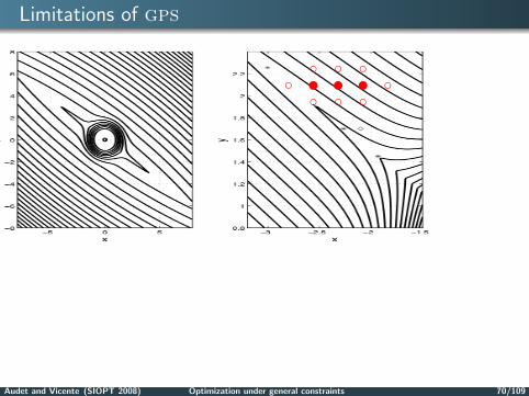
Optimization applied to the meeting logo.
Level sets of f : R2 → R: f(x) =(1− e−‖x‖
2)
max‖x− c‖2, ‖x− d‖2
Audet and Vicente (SIOPT 2008) Optimization under general constraints 70/109

Limitations of gps
u
c cccuc c
cuc ccuc cc c cc
-
6
?
Audet and Vicente (SIOPT 2008) Optimization under general constraints 70/109

Limitations of gps
uc ccc
uc ccuc c
cuc cc c cc-
6
?
For almost all starting points, the iterates of gps with the coordinatedirections converge to a point x on the diagonal, where f is notdifferentiable, with f ′(x;±ei) ≥ 0but f ′(x; d) < 0 with d = (1,−1)T .
Audet and Vicente (SIOPT 2008) Optimization under general constraints 70/109

Limitations of gps
uc cccu
c ccuc c
cuc cc c cc-
6
?
For almost all starting points, the iterates of gps with the coordinatedirections converge to a point x on the diagonal, where f is notdifferentiable, with f ′(x;±ei) ≥ 0but f ′(x; d) < 0 with d = (1,−1)T .
Audet and Vicente (SIOPT 2008) Optimization under general constraints 70/109

Limitations of gps
uc cccuc c
c
uc ccuc cc c cc
-
6
?
For almost all starting points, the iterates of gps with the coordinatedirections converge to a point x on the diagonal, where f is notdifferentiable, with f ′(x;±ei) ≥ 0but f ′(x; d) < 0 with d = (1,−1)T .
Audet and Vicente (SIOPT 2008) Optimization under general constraints 70/109

Limitations of gps
uc cccuc c
cu
c ccuc cc c cc
-
6
?
For almost all starting points, the iterates of gps with the coordinatedirections converge to a point x on the diagonal, where f is notdifferentiable, with f ′(x;±ei) ≥ 0but f ′(x; d) < 0 with d = (1,−1)T .
Audet and Vicente (SIOPT 2008) Optimization under general constraints 70/109
Limitations of gps
uc cccuc c
cuc cc
uc cc c cc-
6
?
For almost all starting points, the iterates of gps with the coordinatedirections converge to a point x on the diagonal, where f is notdifferentiable, with f ′(x;±ei) ≥ 0but f ′(x; d) < 0 with d = (1,−1)T .
Audet and Vicente (SIOPT 2008) Optimization under general constraints 70/109

Limitations of gps
uc cccuc c
cuc ccu
c cc c cc-
6
?
For almost all starting points, the iterates of gps with the coordinatedirections converge to a point x on the diagonal, where f is notdifferentiable, with f ′(x;±ei) ≥ 0but f ′(x; d) < 0 with d = (1,−1)T .
Audet and Vicente (SIOPT 2008) Optimization under general constraints 70/109

Limitations of gps
uc cccuc c
cuc ccuc c
c c cc-
6
?
For almost all starting points, the iterates of gps with the coordinatedirections converge to a point x on the diagonal, where f is notdifferentiable, with f ′(x;±ei) ≥ 0but f ′(x; d) < 0 with d = (1,−1)T .
Audet and Vicente (SIOPT 2008) Optimization under general constraints 70/109

Limitations of gps
uc cccuc c
cuc ccuc cc c cc
-
6
?
For almost all starting points, the iterates of gps with the coordinatedirections converge to a point x on the diagonal, where f is notdifferentiable, with f ′(x;±ei) ≥ 0but f ′(x; d) < 0 with d = (1,−1)T .
Audet and Vicente (SIOPT 2008) Optimization under general constraints 70/109

Limitations of gps - a convex problem
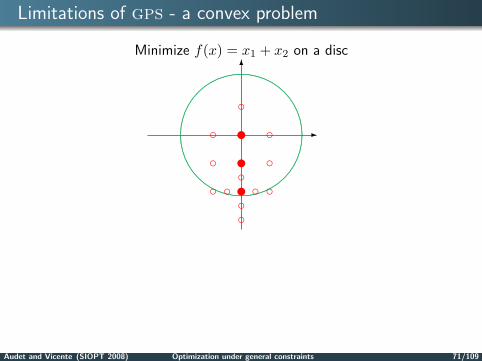
Minimize f(x) = x1 + x2 on a disc6
-....................
...................
...................
...................
..................
..................
....................................
........................................................................................................................................................
..................
..................
..................
..................
...................
...................
...................
..........
.........
..........
.........
...................
...................
...................
..................
..................
..................
..................
................... ................... ................... ................... ................... ......................................
.......................................................
..................
..................
...................
...................
...................
...................
u ccccu cccu ccc
cc ccu -
6
?
Infeasible trial points are simply rejected from consideration.This is called the extreme barrier approach.The gps iterates with the coordinate directions converge to a suboptimalpoint x on the boundary, where f ′(x; +ei) ≥ 0 and x− ei 6∈ Ω.
Audet and Vicente (SIOPT 2008) Optimization under general constraints 71/109

Limitations of gps - a convex problem
Minimize f(x) = x1 + x2 on a disc6
-....................
...................
...................
...................
..................
..................
....................................
........................................................................................................................................................
..................
..................
..................
..................
...................
...................
...................
..........
.........
..........
.........
...................
...................
...................
..................
..................
..................
..................
................... ................... ................... ................... ................... ......................................
.......................................................
..................
..................
...................
...................
...................
...................u
ccccu cccu ccc
cc ccu -
6
?
Infeasible trial points are simply rejected from consideration.This is called the extreme barrier approach.The gps iterates with the coordinate directions converge to a suboptimalpoint x on the boundary, where f ′(x; +ei) ≥ 0 and x− ei 6∈ Ω.
Audet and Vicente (SIOPT 2008) Optimization under general constraints 71/109

Limitations of gps - a convex problem
Minimize f(x) = x1 + x2 on a disc6
-....................
...................
...................
...................
..................
..................
....................................
........................................................................................................................................................
..................
..................
..................
..................
...................
...................
...................
..........
.........
..........
.........
...................
...................
...................
..................
..................
..................
..................
................... ................... ................... ................... ................... ......................................
.......................................................
..................
..................
...................
...................
...................
...................u cccc
u cccu ccc
cc ccu -
6
?
Infeasible trial points are simply rejected from consideration.This is called the extreme barrier approach.The gps iterates with the coordinate directions converge to a suboptimalpoint x on the boundary, where f ′(x; +ei) ≥ 0 and x− ei 6∈ Ω.
Audet and Vicente (SIOPT 2008) Optimization under general constraints 71/109

Limitations of gps - a convex problem
Minimize f(x) = x1 + x2 on a disc6
-....................
...................
...................
...................
..................
..................
....................................
........................................................................................................................................................
..................
..................
..................
..................
...................
...................
...................
..........
.........
..........
.........
...................
...................
...................
..................
..................
..................
..................
................... ................... ................... ................... ................... ......................................
.......................................................
..................
..................
...................
...................
...................
...................u ccccu
cccu ccc
cc ccu -
6
?
Infeasible trial points are simply rejected from consideration.This is called the extreme barrier approach.The gps iterates with the coordinate directions converge to a suboptimalpoint x on the boundary, where f ′(x; +ei) ≥ 0 and x− ei 6∈ Ω.
Audet and Vicente (SIOPT 2008) Optimization under general constraints 71/109

Limitations of gps - a convex problem
Minimize f(x) = x1 + x2 on a disc6
-....................
...................
...................
...................
..................
..................
....................................
........................................................................................................................................................
..................
..................
..................
..................
...................
...................
...................
..........
.........
..........
.........
...................
...................
...................
..................
..................
..................
..................
................... ................... ................... ................... ................... ......................................
.......................................................
..................
..................
...................
...................
...................
...................u ccccu ccc
u ccc
cc ccu -
6
?
Infeasible trial points are simply rejected from consideration.This is called the extreme barrier approach.The gps iterates with the coordinate directions converge to a suboptimalpoint x on the boundary, where f ′(x; +ei) ≥ 0 and x− ei 6∈ Ω.
Audet and Vicente (SIOPT 2008) Optimization under general constraints 71/109

Limitations of gps - a convex problem
Minimize f(x) = x1 + x2 on a disc6
-....................
...................
...................
...................
..................
..................
....................................
........................................................................................................................................................
..................
..................
..................
..................
...................
...................
...................
..........
.........
..........
.........
...................
...................
...................
..................
..................
..................
..................
................... ................... ................... ................... ................... ......................................
.......................................................
..................
..................
...................
...................
...................
...................u ccccu cccu
ccc
cc ccu -
6
?
Infeasible trial points are simply rejected from consideration.This is called the extreme barrier approach.The gps iterates with the coordinate directions converge to a suboptimalpoint x on the boundary, where f ′(x; +ei) ≥ 0 and x− ei 6∈ Ω.
Audet and Vicente (SIOPT 2008) Optimization under general constraints 71/109

Limitations of gps - a convex problem
Minimize f(x) = x1 + x2 on a disc6
-....................
...................
...................
...................
..................
..................
....................................
........................................................................................................................................................
..................
..................
..................
..................
...................
...................
...................
..........
.........
..........
.........
...................
...................
...................
..................
..................
..................
..................
................... ................... ................... ................... ................... ......................................
.......................................................
..................
..................
...................
...................
...................
...................u ccccu cccu ccc
cc ccu -
6
?
Infeasible trial points are simply rejected from consideration.This is called the extreme barrier approach.The gps iterates with the coordinate directions converge to a suboptimalpoint x on the boundary, where f ′(x; +ei) ≥ 0 and x− ei 6∈ Ω.
Audet and Vicente (SIOPT 2008) Optimization under general constraints 71/109
Limitations of gps - a convex problem
Minimize f(x) = x1 + x2 on a disc6
-....................
...................
...................
...................
..................
..................
....................................
........................................................................................................................................................
..................
..................
..................
..................
...................
...................
...................
..........
.........
..........
.........
...................
...................
...................
..................
..................
..................
..................
................... ................... ................... ................... ................... ......................................
.......................................................
..................
..................
...................
...................
...................
...................u ccccu cccu ccc
cc cc
u -
6
?
Infeasible trial points are simply rejected from consideration.This is called the extreme barrier approach.The gps iterates with the coordinate directions converge to a suboptimalpoint x on the boundary, where f ′(x; +ei) ≥ 0 and x− ei 6∈ Ω.
Audet and Vicente (SIOPT 2008) Optimization under general constraints 71/109

Limitations of gps - a convex problem
Minimize f(x) = x1 + x2 on a disc6
-....................
...................
...................
...................
..................
..................
....................................
........................................................................................................................................................
..................
..................
..................
..................
...................
...................
...................
..........
.........
..........
.........
...................
...................
...................
..................
..................
..................
..................
................... ................... ................... ................... ................... ......................................
.......................................................
..................
..................
...................
...................
...................
...................u ccccu cccu ccc
cc ccu -
6
?
Infeasible trial points are simply rejected from consideration.This is called the extreme barrier approach.
The gps iterates with the coordinate directions converge to a suboptimalpoint x on the boundary, where f ′(x; +ei) ≥ 0 and x− ei 6∈ Ω.
Audet and Vicente (SIOPT 2008) Optimization under general constraints 71/109

Limitations of gps - a convex problem
Minimize f(x) = x1 + x2 on a disc6
-....................
...................
...................
...................
..................
..................
....................................
........................................................................................................................................................
..................
..................
..................
..................
...................
...................
...................
..........
.........
..........
.........
...................
...................
...................
..................
..................
..................
..................
................... ................... ................... ................... ................... ......................................
.......................................................
..................
..................
...................
...................
...................
...................u ccccu cccu ccc
cc ccu -
6
?
Infeasible trial points are simply rejected from consideration.This is called the extreme barrier approach.The gps iterates with the coordinate directions converge to a suboptimalpoint x on the boundary, where f ′(x; +ei) ≥ 0 and x− ei 6∈ Ω.
Audet and Vicente (SIOPT 2008) Optimization under general constraints 71/109

Unconstrained nonsmooth optimality conditions
Given any unconstrained optimization problem (NLP ), we desire analgorithm that produces a solution x
Algorithm(NLP ) - x-
Unconstrained optimization hierarchy of optimality conditions :
if f is C1 then 0 = ∇f(x) ⇔ f ′(x; d) ≥ 0 ∀d ∈ Rn
if f is regular then f ′(x; d) ≥ 0 ∀d ∈ Rn
if f is convex then 0 ∈ ∂f(x)if f is Lipschitz near x then 0 ∈ ∂f(x) ⇔ f(x; d) ≥ 0 ∀d ∈ Rn.
Audet and Vicente (SIOPT 2008) Optimization under general constraints 72/109

Clarke derivatives and generalized gradient
Let f be Lipschitz near x ∈ Rn.
The Clarke generalized devivative of f at x in the direction v ∈ Rn is
f(x; v) = lim supy→x, t↓0
f(y + tv)− f(y)t
.
The generalized gradient of f at x is defined to be
∂f(x) = ζ ∈ Rn : f(x; v) ≥ vT ζ for every v ∈ Rn= colim∇f(xi) : xi → x and ∇f(xi) exists .
Properties:
If f is convex, ∂f(x) = sub-gradient.
f is strictly differentiable at x if ∂f(x) contains a single element, andthat element is ∇f(x), and f ′(x; ·) = f(x; ·).
Audet and Vicente (SIOPT 2008) Optimization under general constraints 73/109

Constrained optimization optimality conditions
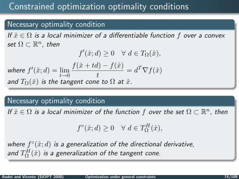
Necessary optimality condition
If x ∈ Ω is a local minimizer of a differentiable function f over a convexset Ω ⊂ Rn, then
f ′(x; d) ≥ 0 ∀ d ∈ TΩ(x),
where f ′(x; d) = limt→0
f(x + td)− f(x)t
= dT∇f(x)
and TΩ(x) is the tangent cone to Ω at x.
Necessary optimality condition
If x ∈ Ω is a local minimizer of the function f over the set Ω ⊂ Rn, then
f(x; d) ≥ 0 ∀ d ∈ THΩ (x),
where f(x; d) is a generalization of the directional derivative,and TH
Ω (x) is a generalization of the tangent cone.
Audet and Vicente (SIOPT 2008) Optimization under general constraints 74/109
Constrained optimization optimality conditions
Necessary optimality condition
If x ∈ Ω is a local minimizer of a differentiable function f over a convexset Ω ⊂ Rn, then
f ′(x; d) ≥ 0 ∀ d ∈ TΩ(x),
where f ′(x; d) = limt→0
f(x + td)− f(x)t
= dT∇f(x)
and TΩ(x) is the tangent cone to Ω at x.
Necessary optimality condition
If x ∈ Ω is a local minimizer of the function f over the set Ω ⊂ Rn, then
f(x; d) ≥ 0 ∀ d ∈ THΩ (x),
where f(x; d) is a generalization of the directional derivative,and TH
Ω (x) is a generalization of the tangent cone.
Audet and Vicente (SIOPT 2008) Optimization under general constraints 74/109

Extending gps to handle nonlinear constraints
For unconstrained optimization, gps garantees(under a local Lipschitz assumption) to produce a limit point x suchthat f(x; d) ≥ 0 for every d used infinitely often.Unfortunately, the d’s are selected from a fixed finite set D, and gpsmay miss important directions. The effect is more pronounced as thedimension increases.
Torczon and Lewis show how to adapt gps to explicit bound or linearinequalities. The directions in D are constructed using the nearbyactive constraints.
gps is not suited for nonlinear constraints.
Recently, Kolda, Lewis and Torczon proposed an augmentedLagrangean gss approach, analyzed under the assumption that theobjective and constraints be twice continuously differentiable.
Mads generalizes gps by allowing more directions. Mads isdesigned for both constrained or unconstrained optimization, anddoes not require any smoothness assumptions.
Audet and Vicente (SIOPT 2008) Optimization under general constraints 75/109

From Coordinate Search to OrthoMads
OrthoMads – 2008
uxk
Audet and Vicente (SIOPT 2008) Optimization under general constraints 76/109

From Coordinate Search to OrthoMads
OrthoMads – 2008
uxk
up1
up2
up3
up4
HHHHH
HHHHH
HH
Audet and Vicente (SIOPT 2008) Optimization under general constraints 76/109

From Coordinate Search to OrthoMads
OrthoMads – 2008
uxk
Audet and Vicente (SIOPT 2008) Optimization under general constraints 76/109

From Coordinate Search to OrthoMads
OrthoMads – 2008
uxk uu
u uJ
JJ
JJ
J
Audet and Vicente (SIOPT 2008) Optimization under general constraints 76/109

From Coordinate Search to OrthoMads
OrthoMads – 2008
uxk
Audet and Vicente (SIOPT 2008) Optimization under general constraints 76/109

From Coordinate Search to OrthoMads
OrthoMads – 2008
uxku
u uu
ZZ
ZZ
Audet and Vicente (SIOPT 2008) Optimization under general constraints 76/109
From Coordinate Search to OrthoMads
OrthoMads – 2008
uxku
u uu
ZZ
ZZ
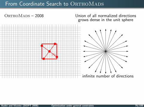
Union of all normalized directionsgrows dense in the unit sphere
6
?
-
@@@@@R
@@
@@@I
AAAAAAU
HHHH
HHY
AAAAAAK
*
HHHHHHj
CCCCCCO
CCCCCCW
:
XXXXXXz
XXXX
XXy
9
infinite number of directions
Audet and Vicente (SIOPT 2008) Optimization under general constraints 76/109

From Coordinate Search to OrthoMads
OrthoMads – 2008
uxku
u uu
ZZ
ZZ
Union of all normalized directionsgrows dense in the unit sphere
6
?
-
@@@@@R
@@
@@@I
AAAAAAU
HHHH
HHY
AAAAAAK
*
HHHHHHj
CCCCCCO
CCCCCCW
:
XXXXXXz
XXXX
XXy
9
infinite number of directions
OrthoMads is deterministic.Results are reproducible on any machine.
At any given iteration, the directions are orthogonal.
Audet and Vicente (SIOPT 2008) Optimization under general constraints 76/109
OrthoMads: Halton Pseudo-random sequence
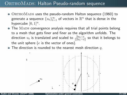
OrthoMads uses the pseudo-random Halton sequence (1960) togenerate a sequence ut∞t=1 of vectors in Rn that is dense in thehypercube [0, 1]n.The Mads convergence analysis requires that all trial points belongto a mesh that gets finer and finer as the algorithm unfolds. Thedirection ut is translated and scaled to 2ut−e
‖2ut−e‖ so that it belongs to
the unit sphere (e is the vector of ones).The direction is rounded to the nearest mesh direction q.
Audet and Vicente (SIOPT 2008) Optimization under general constraints 77/109

OrthoMads: Householder orthogonal matrix
The Householder transformation is then applied to the integerdirection q:
H = ‖q‖2In − 2qqT ,
where In is the identity matrix.
By construction, H is an integer orthogonal basis of Rn.
The poll directions for OrthoMads are defined to be the columns ofH and −H.
A lower bound on the cosine of the maximum angle between anyarbitrary nonzero vector v ∈ Rn and the set of directions in D isdefined as
κ(D) = min0 6=v∈Rn
maxd∈D
vT d
‖v‖‖d‖.
With OrthoMads the measure κ(D) = 1√n
is maximized over all
positive bases.
Audet and Vicente (SIOPT 2008) Optimization under general constraints 78/109

Convergence analysis - OrthoMads with extreme barrier
Theorem
As k →∞, the set of OrthoMads normalized poll directions is dense inthe unit sphere.
Theorem
Let x be the the limit of a subsequence of mesh local optimizers onmeshes that get infinitely fine. If f is Lipschitz near x,then f(x, v) ≥ 0 for all v ∈ TH
Ω (x).
Assuming more smoothness, Abramson studies second order convergence.
Audet and Vicente (SIOPT 2008) Optimization under general constraints 79/109

Convergence analysis - OrthoMads with extreme barrier
Theorem
As k →∞, the set of OrthoMads normalized poll directions is dense inthe unit sphere.
Theorem
Let x be the the limit of a subsequence of mesh local optimizers onmeshes that get infinitely fine. If f is Lipschitz near x,then f(x, v) ≥ 0 for all v ∈ TH
Ω (x).
Assuming more smoothness, Abramson studies second order convergence.Audet and Vicente (SIOPT 2008) Optimization under general constraints 79/109

Open, closed and hidden constraints
Consider the toy problem: minx∈R2
x21 −√
x2
s.t. −x21 + x2
2 ≤ 1x2 ≥ 0
Closed constraints must be satisfied at every trial vector of decisionvariables in order for the functions to evaluate.Here x2 ≥ 0 is a closed constraint, because if it is violated, theobjective function will fail.
Open constraints must be satisfied at the solution, but anoptimization algorithm may generate iterates that violate it. Here−x2
1 + x22 ≤ 1 is an open constraint.
Lets change the objective. x2 6= 0 is now an hidden constraint.f is set to ∞ when x ∈ Ω but x fails to satisfy an hidden contraint.
This terminology differs from soft and hard constraints which meanthat satisfaction might allow, or might not, for some tolerance on theright hand side of cj(x) ≤ 0.
Audet and Vicente (SIOPT 2008) Optimization under general constraints 80/109

Open, closed and hidden constraints
Consider the toy problem: minx∈R2
x21− ln(x2)
s.t. −x21 + x2
2 ≤ 1x2 ≥ 0
Closed constraints must be satisfied at every trial vector of decisionvariables in order for the functions to evaluate.Here x2 ≥ 0 is a closed constraint, because if it is violated, theobjective function will fail.
Open constraints must be satisfied at the solution, but anoptimization algorithm may generate iterates that violate it. Here−x2
1 + x22 ≤ 1 is an open constraint.
Lets change the objective. x2 6= 0 is now an hidden constraint.f is set to ∞ when x ∈ Ω but x fails to satisfy an hidden contraint.
This terminology differs from soft and hard constraints which meanthat satisfaction might allow, or might not, for some tolerance on theright hand side of cj(x) ≤ 0.
Audet and Vicente (SIOPT 2008) Optimization under general constraints 80/109

Constrained optimization
Consider the constrained problem
minx∈Ω
f(x)
where f : Rn → R ∪ ∞and Ω = x ∈ X ⊂ Rn : C(x) ≤ 0 with C : Rn → (R ∪ ∞)m.
Hypothesis
An initial x0 ∈ X with f(x0) <∞, and C(x) <∞ is provided.
Audet and Vicente (SIOPT 2008) Optimization under general constraints 81/109

Constrained optimization
Consider the constrained problem
minx∈Ω
f(x)
where f : Rn → R ∪ ∞and Ω = x ∈ X ⊂ Rn : C(x) ≤ 0 with C : Rn → (R ∪ ∞)m.
Hypothesis
An initial x0 ∈ X with f(x0) <∞, and C(x) <∞ is provided.
Audet and Vicente (SIOPT 2008) Optimization under general constraints 81/109

Filter approach to constraints (Based on Fletcher - Leyffer)
minx∈Ω
f(x)
The extreme barrier handles the closed and hidden constraints X.A filter handles C(x) ≤ 0.
Define the nonnegative constraint violation function
h(x) :=
∑
j
max(0, cj(x))2if x ∈ X and
f(x) <∞,⇐ open constraints
+∞ otherwise. ⇐ closed constraints
h(x) = 0 if and only if x ∈ Ω.The constrained optimization problem is then viewed as a biobjective one:to minimize f and h, with a priority to h. This allows trial points thatviolate the open constraints.
Audet and Vicente (SIOPT 2008) Optimization under general constraints 82/109

Filter approach to constraints
..........................
.......................
......................
....................... ........................ ........................ ......................... .......................... ........................... .............................. ................................................................... ..............................
..........................
.......................
...................
................ ............. ........... .......... ........ ........ ...................................................
...................
......................
.........................
............................
. .................................................................
............................................................................................................................................................................................
...................
..................................
..............................
............................
.........................
.......................
.............
.......
.............
......
..................
.................................
................ ................. ................... ..................... ....................... ......................... ........................... ............................. ................................ ................................... .................................................................................
Ω
X
sxI
6f
-h
ssxF
s.
.........................
................................................
....................... ....................... ....................... ........................ ..................................................
......................
........
..............................
..............................
.
............................
..................................................................................................................................................................
.......................................................................................................................................................................................................................................
................................
................
...................
.......................................................................
...............................
....................
..............
...........................................................................
.
..............................
............................
.........................
.......................
....................
......................................................@
@I
Optimal solution
•
•h=0
h=3
.
.......................................
....................................
................................
.............................
..........................
.......................
....................
.................
...........................................................................
................
...................
......................
..........................
.
.................
..............
................................ ...... ........ .......... ............
...............
..................
......................
.........................
............................
...............................
h=2.
..........
..........
.....
..........
..........
..
..........
........
..........
.....
..........
..................................................
...........................
...................
......................
.........................
............................ •
•
BBBBBBBBBBBBN
Local min of h
Audet and Vicente (SIOPT 2008) Optimization under general constraints 83/109

Filter approach to constraints
..........................
.......................
......................
....................... ........................ ........................ ......................... .......................... ........................... .............................. ................................................................... ..............................
..........................
.......................
...................
................ ............. ........... .......... ........ ........ ...................................................
...................
......................
.........................
............................
. .................................................................
............................................................................................................................................................................................
...................
..................................
..............................
............................
.........................
.......................
.............
.......
.............
......
..................
.................................
................ ................. ................... ..................... ....................... ......................... ........................... ............................. ................................ ................................... .................................................................................
Ω
X
sxI
6f
-h
. ........................................ ...................................... ...................................... ...................................... .....................................................................
........
.......................................
.......................................
....................................
...
................................
.......
............................
........... s(h(xI ,f(xI))
sxF
s.
.........................
................................................
....................... ....................... ....................... ........................ ..................................................
......................
........
..............................
..............................
.
............................
..................................................................................................................................................................
.......................................................................................................................................................................................................................................
................................
................
...................
.......................................................................
...............................
....................
..............
...........................................................................
.
..............................
............................
.........................
.......................
....................
......................................................@
@I
Optimal solution
•
•h=0
h=3
.
.......................................
....................................
................................
.............................
..........................
.......................
....................
.................
...........................................................................
................
...................
......................
..........................
.
.................
..............
................................ ...... ........ .......... ............
...............
..................
......................
.........................
............................
...............................
h=2.
..........
..........
.....
..........
..........
..
..........
........
..........
.....
..........
..................................................
...........................
...................
......................
.........................
............................ •
•
BBBBBBBBBBBBN
Local min of h
Audet and Vicente (SIOPT 2008) Optimization under general constraints 83/109

Filter approach to constraints
..........................
.......................
......................
....................... ........................ ........................ ......................... .......................... ........................... .............................. ................................................................... ..............................
..........................
.......................
...................
................ ............. ........... .......... ........ ........ ...................................................
...................
......................
.........................
............................
. .................................................................
............................................................................................................................................................................................
...................
..................................
..............................
............................
.........................
.......................
.............
.......
.............
......
..................
.................................
................ ................. ................... ..................... ....................... ......................... ........................... ............................. ................................ ................................... .................................................................................
Ω
X
sxI
6f
-h
s(h(xI ,f(xI))s
xF
s.
.........................
................................................
....................... ....................... ....................... ........................ ..................................................
......................
........
..............................
..............................
.
............................
..................................................................................................................................................................
.......................................................................................................................................................................................................................................
................................
................
...................
.......................................................................
...............................
....................
..............
...........................................................................
.
..............................
............................
.........................
.......................
....................
......................................................@
@I
Optimal solution
•
•h=0
h=3
.
.......................................
....................................
................................
.............................
..........................
.......................
....................
.................
...........................................................................
................
...................
......................
..........................
.
.................
..............
................................ ...... ........ .......... ............
...............
..................
......................
.........................
............................
...............................
h=2.
..........
..........
.....
..........
..........
..
..........
........
..........
.....
..........
..................................................
...........................
...................
......................
.........................
............................ •
•
BBBBBBBBBBBBN
Local min of h
Audet and Vicente (SIOPT 2008) Optimization under general constraints 83/109

Filter approach to constraints
..........................
.......................
......................
....................... ........................ ........................ ......................... .......................... ........................... .............................. ................................................................... ..............................
..........................
.......................
...................
................ ............. ........... .......... ........ ........ ...................................................
...................
......................
.........................
............................
. .................................................................
............................................................................................................................................................................................
...................
..................................
..............................
............................
.........................
.......................
.............
.......
.............
......
..................
.................................
................ ................. ................... ..................... ....................... ......................... ........................... ............................. ................................ ................................... .................................................................................
Ω
X
sxI
6f
-h
s(h(xI ,f(xI))s
xF.
.............................................
...........................................
........................................
......................................
....................................
................................................................
....................................................... ........................ ....................... ...................... ......................
.....................
.....................
.....................
(h(xF ,f(xF ))s
..........................
................................................
....................... ....................... ....................... ........................ ..................................................
......................
........
..............................
..............................
.
............................
..................................................................................................................................................................
.......................................................................................................................................................................................................................................
................................
................
...................
.......................................................................
...............................
....................
..............
...........................................................................
.
..............................
............................
.........................
.......................
....................
......................................................@
@I
Optimal solution
•
•h=0
h=3
.
.......................................
....................................
................................
.............................
..........................
.......................
....................
.................
...........................................................................
................
...................
......................
..........................
.
.................
..............
................................ ...... ........ .......... ............
...............
..................
......................
.........................
............................
...............................
h=2.
..........
..........
.....
..........
..........
..
..........
........
..........
.....
..........
..................................................
...........................
...................
......................
.........................
............................ •
•
BBBBBBBBBBBBN
Local min of h
Audet and Vicente (SIOPT 2008) Optimization under general constraints 83/109

Filter approach to constraints
..........................
.......................
......................
....................... ........................ ........................ ......................... .......................... ........................... .............................. ................................................................... ..............................
..........................
.......................
...................
................ ............. ........... .......... ........ ........ ...................................................
...................
......................
.........................
............................
. .................................................................
............................................................................................................................................................................................
...................
..................................
..............................
............................
.........................
.......................
.............
.......
.............
......
..................
.................................
................ ................. ................... ..................... ....................... ......................... ........................... ............................. ................................ ................................... .................................................................................
Ω
X
sxI
6f
-h
ssxF
s.
.........................
................................................
....................... ....................... ....................... ........................ ..................................................
......................
........
..............................
..............................
.
............................
..................................................................................................................................................................
.......................................................................................................................................................................................................................................
................................
................
...................
.......................................................................
...............................
....................
..............
...........................................................................
(h(X), f(X))
.
..............................
............................
.........................
.......................
....................
......................................................@
@I
Optimal solution
•
•h=0
h=3
.
.......................................
....................................
................................
.............................
..........................
.......................
....................
.................
...........................................................................
................
...................
......................
..........................
.
.................
..............
................................ ...... ........ .......... ............
...............
..................
......................
.........................
............................
...............................
h=2.
..........
..........
.....
..........
..........
..
..........
........
..........
.....
..........
..................................................
...........................
...................
......................
.........................
............................ •
•
BBBBBBBBBBBBN
Local min of h
Audet and Vicente (SIOPT 2008) Optimization under general constraints 83/109
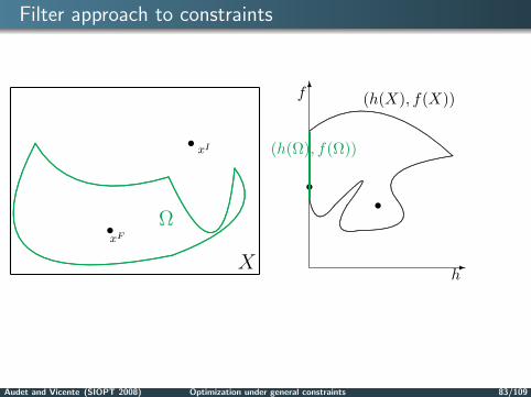
Filter approach to constraints
..........................
.......................
......................
....................... ........................ ........................ ......................... .......................... ........................... .............................. ................................................................... ..............................
..........................
.......................
...................
................ ............. ........... .......... ........ ........ ...................................................
...................
......................
.........................
............................
. .................................................................
............................................................................................................................................................................................
...................
..................................
..............................
............................
.........................
.......................
.............
.......
.............
......
..................
.................................
................ ................. ................... ..................... ....................... ......................... ........................... ............................. ................................ ................................... .................................................................................
Ω
X
sxI
6f
-h
ssxF
s.
.........................
................................................
....................... ....................... ....................... ........................ ..................................................
......................
........
..............................
..............................
.
............................
..................................................................................................................................................................
.......................................................................................................................................................................................................................................
................................
................
...................
.......................................................................
...............................
....................
..............
...........................................................................
(h(X), f(X))
(h(Ω), f(Ω))
.
..............................
............................
.........................
.......................
....................
......................................................@
@I
Optimal solution
•
•h=0
h=3
.
.......................................
....................................
................................
.............................
..........................
.......................
....................
.................
...........................................................................
................
...................
......................
..........................
.
.................
..............
................................ ...... ........ .......... ............
...............
..................
......................
.........................
............................
...............................
h=2.
..........
..........
.....
..........
..........
..
..........
........
..........
.....
..........
..................................................
...........................
...................
......................
.........................
............................ •
•
BBBBBBBBBBBBN
Local min of h
Audet and Vicente (SIOPT 2008) Optimization under general constraints 83/109

Filter approach to constraints
..........................
.......................
......................
....................... ........................ ........................ ......................... .......................... ........................... .............................. ................................................................... ..............................
..........................
.......................
...................
................ ............. ........... .......... ........ ........ ...................................................
...................
......................
.........................
............................
. .................................................................
............................................................................................................................................................................................
...................
..................................
..............................
............................
.........................
.......................
.............
.......
.............
......
..................
.................................
................ ................. ................... ..................... ....................... ......................... ........................... ............................. ................................ ................................... .................................................................................
Ω
X
sxI
6f
-h
ssxF
s.
.........................
................................................
....................... ....................... ....................... ........................ ..................................................
......................
........
..............................
..............................
.
............................
..................................................................................................................................................................
.......................................................................................................................................................................................................................................
................................
................
...................
.......................................................................
...............................
....................
..............
...........................................................................
.
..............................
............................
.........................
.......................
....................
......................................................@
@I
Optimal solution
•
•
h=0
h=3
.
.......................................
....................................
................................
.............................
..........................
.......................
....................
.................
...........................................................................
................
...................
......................
..........................
.
.................
..............
................................ ...... ........ .......... ............
...............
..................
......................
.........................
............................
...............................
h=2.
..........
..........
.....
..........
..........
..
..........
........
..........
.....
..........
..................................................
...........................
...................
......................
.........................
............................ •
•
BBBBBBBBBBBBN
Local min of h
Audet and Vicente (SIOPT 2008) Optimization under general constraints 83/109
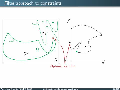
Filter approach to constraints
..........................
.......................
......................
....................... ........................ ........................ ......................... .......................... ........................... .............................. ................................................................... ..............................
..........................
.......................
...................
................ ............. ........... .......... ........ ........ ...................................................
...................
......................
.........................
............................
. .................................................................
............................................................................................................................................................................................
...................
..................................
..............................
............................
.........................
.......................
.............
.......
.............
......
..................
.................................
................ ................. ................... ..................... ....................... ......................... ........................... ............................. ................................ ................................... .................................................................................
Ω
X
sxI
6f
-h
ssxF
s.
.........................
................................................
....................... ....................... ....................... ........................ ..................................................
......................
........
..............................
..............................
.
............................
..................................................................................................................................................................
.......................................................................................................................................................................................................................................
................................
................
...................
.......................................................................
...............................
....................
..............
...........................................................................
.
..............................
............................
.........................
.......................
....................
......................................................@
@I
Optimal solution
•
•h=0
h=3
.
.......................................
....................................
................................
.............................
..........................
.......................
....................
.................
...........................................................................
................
...................
......................
..........................
.
.................
..............
................................ ...... ........ .......... ............
...............
..................
......................
.........................
............................
...............................
h=2.
..........
..........
.....
..........
..........
..
..........
........
..........
.....
..........
..................................................
...........................
...................
......................
.........................
............................ •
•
BBBBBBBBBBBBN
Local min of h
Audet and Vicente (SIOPT 2008) Optimization under general constraints 83/109

Filter approach to constraints
..........................
.......................
......................
....................... ........................ ........................ ......................... .......................... ........................... .............................. ................................................................... ..............................
..........................
.......................
...................
................ ............. ........... .......... ........ ........ ...................................................
...................
......................
.........................
............................
. .................................................................
............................................................................................................................................................................................
...................
..................................
..............................
............................
.........................
.......................
.............
.......
.............
......
..................
.................................
................ ................. ................... ..................... ....................... ......................... ........................... ............................. ................................ ................................... .................................................................................
Ω
X
sxI
6f
-h
ssxF
s.
.........................
................................................
....................... ....................... ....................... ........................ ..................................................
......................
........
..............................
..............................
.
............................
..................................................................................................................................................................
.......................................................................................................................................................................................................................................
................................
................
...................
.......................................................................
...............................
....................
..............
...........................................................................
.
..............................
............................
.........................
.......................
....................
......................................................@
@I
Optimal solution
•
•h=0
h=3
.
.......................................
....................................
................................
.............................
..........................
.......................
....................
.................
...........................................................................
................
...................
......................
..........................
.
.................
..............
................................ ...... ........ .......... ............
...............
..................
......................
.........................
............................
...............................
h=2.
..........
..........
.....
..........
..........
..
..........
........
..........
.....
..........
..................................................
...........................
...................
......................
.........................
............................ •
•
BBBBBBBBBBBBN
Local min of h
Audet and Vicente (SIOPT 2008) Optimization under general constraints 83/109

A Mads algorithm with a progressive barrier
We present an algorithm that
At iteration k, any trial point whose constraint violation value exceedsthe value hmax
k is discarded from consideration.
As k increases, the threshold hmaxk is reduced.
The algorithm accepts some trial points that violate the openconstraints.
Audet and Vicente (SIOPT 2008) Optimization under general constraints 84/109

Progressive barrier algorithm : Iteration 0
..........................
.......................
......................
....................... ........................ ........................ ......................... .......................... ........................... .............................. ................................................................... ..............................
..........................
.......................
...................
................ ............. ........... .......... ........ ........ ...................................................
...................
......................
.........................
............................
. .................................................................
............................................................................................................................................................................................
...................
..................................
..............................
............................
.........................
.......................
.............
.......
.............
......
..................
.................................
................ ................. ................... ..................... ....................... ......................... ........................... ............................. ................................ ................................... .................................................................................
Ω
X
sx0
6f
-h
hmax0
s
Audet and Vicente (SIOPT 2008) Optimization under general constraints 85/109

Progressive barrier algorithm : Iteration 0
..........................
.......................
......................
....................... ........................ ........................ ......................... .......................... ........................... .............................. ................................................................... ..............................
..........................
.......................
...................
................ ............. ........... .......... ........ ........ ...................................................
...................
......................
.........................
............................
. .................................................................
............................................................................................................................................................................................
...................
..................................
..............................
............................
.........................
.......................
.............
.......
.............
......
..................
.................................
................ ................. ................... ..................... ....................... ......................... ........................... ............................. ................................ ................................... .................................................................................
Ω
X
sx0
6f
-h
hmax0
....................................................
..................................................................................................
.............................................. ............................................. ............................................. ............................................. .................................................................................
..........
..............................................
..............................................
..........................................
.....
....................................
...........
................................
...............
..............................
..................
..........................
...................... s
Audet and Vicente (SIOPT 2008) Optimization under general constraints 85/109

Progressive barrier algorithm : Iteration 0
..........................
.......................
......................
....................... ........................ ........................ ......................... .......................... ........................... .............................. ................................................................... ..............................
..........................
.......................
...................
................ ............. ........... .......... ........ ........ ...................................................
...................
......................
.........................
............................
. .................................................................
............................................................................................................................................................................................
...................
..................................
..............................
............................
.........................
.......................
.............
.......
.............
......
..................
.................................
................ ................. ................... ..................... ....................... ......................... ........................... ............................. ................................ ................................... .................................................................................
Ω
X
sx0
6f
-h
hmax0
s
Audet and Vicente (SIOPT 2008) Optimization under general constraints 85/109

Progressive barrier algorithm : Iteration 0
..........................
.......................
......................
....................... ........................ ........................ ......................... .......................... ........................... .............................. ................................................................... ..............................
..........................
.......................
...................
................ ............. ........... .......... ........ ........ ...................................................
...................
......................
.........................
............................
. .................................................................
............................................................................................................................................................................................
...................
..................................
..............................
............................
.........................
.......................
.............
.......
.............
......
..................
.................................
................ ................. ................... ..................... ....................... ......................... ........................... ............................. ................................ ................................... .................................................................................
Ω
X
sx0
6f
-h
hmax0
s
c
cc cs
s.
.............................................
........................................................................................
........................................... ........................................... ........................................... ............................................. .....................................................................................
.........
..................................................
...................................................
..............................................
.......
..........................................
............
......................................
..................
Worst h and worst f
Audet and Vicente (SIOPT 2008) Optimization under general constraints 85/109

Progressive barrier algorithm : Iteration 0
..........................
.......................
......................
....................... ........................ ........................ ......................... .......................... ........................... .............................. ................................................................... ..............................
..........................
.......................
...................
................ ............. ........... .......... ........ ........ ...................................................
...................
......................
.........................
............................
. .................................................................
............................................................................................................................................................................................
...................
..................................
..............................
............................
.........................
.......................
.............
.......
.............
......
..................
.................................
................ ................. ................... ..................... ....................... ......................... ........................... ............................. ................................ ................................... .................................................................................
Ω
X
sx0
6f
-h
hmax0
s
c
cc cs
s
sOutside closed constraints X : reject point (barrier approach)
Audet and Vicente (SIOPT 2008) Optimization under general constraints 85/109
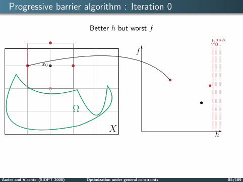
Progressive barrier algorithm : Iteration 0
..........................
.......................
......................
....................... ........................ ........................ ......................... .......................... ........................... .............................. ................................................................... ..............................
..........................
.......................
...................
................ ............. ........... .......... ........ ........ ...................................................
...................
......................
.........................
............................
. .................................................................
............................................................................................................................................................................................
...................
..................................
..............................
............................
.........................
.......................
.............
.......
.............
......
..................
.................................
................ ................. ................... ..................... ....................... ......................... ........................... ............................. ................................ ................................... .................................................................................
Ω
X
sx0
6f
-h
hmax0
s
c
cc cs
s
ss
s.
............................................................
...............................................................................................................
................................................................................................... ............................................. .......................................... ........................................ ....................................... ..................................... ...................................
..................................
................................
...............................
.............................
............................
........................
..
Better h but worst f
Audet and Vicente (SIOPT 2008) Optimization under general constraints 85/109

Progressive barrier algorithm : Iteration 0
..........................
.......................
......................
....................... ........................ ........................ ......................... .......................... ........................... .............................. ................................................................... ..............................
..........................
.......................
...................
................ ............. ........... .......... ........ ........ ...................................................
...................
......................
.........................
............................
. .................................................................
............................................................................................................................................................................................
...................
..................................
..............................
............................
.........................
.......................
.............
.......
.............
......
..................
.................................
................ ................. ................... ..................... ....................... ......................... ........................... ............................. ................................ ................................... .................................................................................
Ω
X
sx0
6f
-h
hmax0
s
ss
ss
sss
................................................
.............................................
..........................................
..............................................................................
...................................................................... ................................ ............................... ............................... ...............................
...............................
...............................
..............................
..............................
..........................
....
........................
........
...................................
.....................................
Better h and better f
Audet and Vicente (SIOPT 2008) Optimization under general constraints 85/109

Progressive barrier algorithm : Iteration 0
..........................
.......................
......................
....................... ........................ ........................ ......................... .......................... ........................... .............................. ................................................................... ..............................
..........................
.......................
...................
................ ............. ........... .......... ........ ........ ...................................................
...................
......................
.........................
............................
. .................................................................
............................................................................................................................................................................................
...................
..................................
..............................
............................
.........................
.......................
.............
.......
.............
......
..................
.................................
................ ................. ................... ..................... ....................... ......................... ........................... ............................. ................................ ................................... .................................................................................
Ω
X
sx0
6f
-h
hmax0
s
ss
ss
sss
The new infeasible incumbent is the one to the left(in (h, f) plot) of the last one with the best f value
x1
hmax1
If time > 11h35, then Skip 12 clicks
Audet and Vicente (SIOPT 2008) Optimization under general constraints 85/109

Progressive barrier algorithm : Iteration 1
..........................
.......................
......................
....................... ........................ ........................ ......................... .......................... ........................... .............................. ................................................................... ..............................
..........................
.......................
...................
................ ............. ........... .......... ........ ........ ...................................................
...................
......................
.........................
............................
. .................................................................
............................................................................................................................................................................................
...................
..................................
..............................
............................
.........................
.......................
.............
.......
.............
......
..................
.................................
................ ................. ................... ..................... ....................... ......................... ........................... ............................. ................................ ................................... .................................................................................
Ω
X
ss
cx1
hmax1
6f
-h
................................................
.............................................
..........................................
..............................................................................
...................................................................... ................................ ............................... ............................... ...............................
...............................
...............................
..............................
..............................
..........................
....
........................
........
...................................
.....................................
Audet and Vicente (SIOPT 2008) Optimization under general constraints 86/109

Progressive barrier algorithm : Iteration 1
..........................
.......................
......................
....................... ........................ ........................ ......................... .......................... ........................... .............................. ................................................................... ..............................
..........................
.......................
...................
................ ............. ........... .......... ........ ........ ...................................................
...................
......................
.........................
............................
. .................................................................
............................................................................................................................................................................................
...................
..................................
..............................
............................
.........................
.......................
.............
.......
.............
......
..................
.................................
................ ................. ................... ..................... ....................... ......................... ........................... ............................. ................................ ................................... .................................................................................
Ω
X
ss
cx1
hmax1
6f
-h
c
cc c
s
ss s
s sss
Audet and Vicente (SIOPT 2008) Optimization under general constraints 86/109
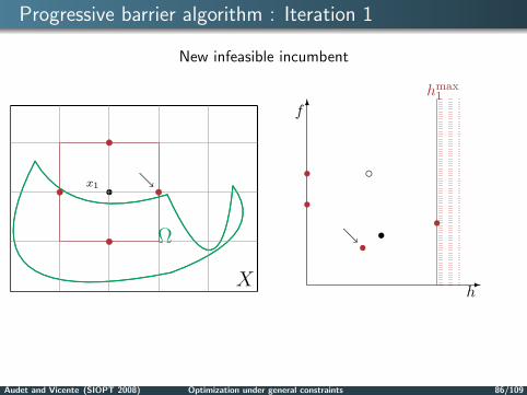
Progressive barrier algorithm : Iteration 1
..........................
.......................
......................
....................... ........................ ........................ ......................... .......................... ........................... .............................. ................................................................... ..............................
..........................
.......................
...................
................ ............. ........... .......... ........ ........ ...................................................
...................
......................
.........................
............................
. .................................................................
............................................................................................................................................................................................
...................
..................................
..............................
............................
.........................
.......................
.............
.......
.............
......
..................
.................................
................ ................. ................... ..................... ....................... ......................... ........................... ............................. ................................ ................................... .................................................................................
Ω
X
ss
cx1
hmax1
6f
-h
c
cc c
s
ss s
s sss
New infeasible incumbent
Audet and Vicente (SIOPT 2008) Optimization under general constraints 86/109

Progressive barrier algorithm : Iteration 1
..........................
.......................
......................
....................... ........................ ........................ ......................... .......................... ........................... .............................. ................................................................... ..............................
..........................
.......................
...................
................ ............. ........... .......... ........ ........ ...................................................
...................
......................
.........................
............................
. .................................................................
............................................................................................................................................................................................
...................
..................................
..............................
............................
.........................
.......................
.............
.......
.............
......
..................
.................................
................ ................. ................... ..................... ....................... ......................... ........................... ............................. ................................ ................................... .................................................................................
Ω
X
ss
cx1
hmax1
6f
-h
c
cc c
s
ss s
s sss
New feasible incumbent
Audet and Vicente (SIOPT 2008) Optimization under general constraints 86/109

Progressive barrier algorithm : Iteration 2
..........................
.......................
......................
....................... ........................ ........................ ......................... .......................... ........................... .............................. ................................................................... ..............................
..........................
.......................
...................
................ ............. ........... .......... ........ ........ ...................................................
...................
......................
.........................
............................
. .................................................................
............................................................................................................................................................................................
...................
..................................
..............................
............................
.........................
.......................
.............
.......
.............
......
..................
.................................
................ ................. ................... ..................... ....................... ......................... ........................... ............................. ................................ ................................... ................................................................................. X
ss
xF2
ss
xI2
hmax2
6f
-h
hmaxk progressively decreases
Audet and Vicente (SIOPT 2008) Optimization under general constraints 87/109
Convergence analysis of OrthoMads under theprogressive barrier
Assumptions
At least one initial point in X is provided – but not required to be inΩ.
All iterates belong to some compact set – it is sufficient to assumethat level sets of f in X are bounded.
Theorem
As k →∞, OrthoMads’s normalized polling directions form a dense setin the unit sphere.
Audet and Vicente (SIOPT 2008) Optimization under general constraints 88/109

Limit of feasible poll centers
Theorem
Let x ∈ Ω be the limit of unsuccessful feasible poll centers xFk on
meshes that get infinitely fine. If f is Lipschitz near x,then f(x, v) ≥ 0 for all v ∈ TH
Ω (x).
Corollary
In addition, if f is strictly differentiable near x, and if Ω is regular near x,then f ′(x, v) ≥ 0 for all v ∈ TΩ(x), i.e., x is a KKT point for min
x∈Ωf(x).
Audet and Vicente (SIOPT 2008) Optimization under general constraints 89/109
Limit of infeasible poll centers
Theorem
Let x ∈ X be the limit of unsuccessful infeasible poll centers xIk on
meshes that get infinitely fine. If h is Lipschitz near x,then h(x, v) ≥ 0 for all v ∈ TH
X (x).
Corollary
In addition, if h is strictly differentiable near x, and if X is regular near x,then h′(x, v) ≥ 0 for all v ∈ TX(x) i.e., x is a KKT point for min
x∈Xh(x).
Audet and Vicente (SIOPT 2008) Optimization under general constraints 90/109

Equality constraints
All the above ideas dealt with inequality constraints.
Dreisigmeyer recently proposed to construct a mesh using geodesics ofthe Riemannian manifold formed by equalities (not necessarily linear).Knowledge of the equalities is necessary.
-
6
x3
x1
x2
.
.......................................
....................................
.................................
..............................
...........................
........................
.....................
....................
.........................
.....................
.............................................
.............................................
..............................................
......................................................................................................................................................................................................................................................................................
............................
........................
................................................
.................................................
. ..................... ...................... ....................... .......................... ............................ . .......................................... ....................................... .................................... ................................. .............................. ........................... ......................... ........................ ...................... ........................................................
Manifold
∗
∗ poll center xk
.......................................................... . ................
................
...................
.....................
........................
. ...................... ........................ ............................ ............................... .................................. ..................................... ........................................ . ...................... ......................... ........................... .............................. .................................. .............................................................................• ••
•
• poll points
Audet and Vicente (SIOPT 2008) Optimization under general constraints 91/109

Presentation outline
1 Introduction
2 Unconstrained optimization
3 Optimization under general constraints
4 Surrogates, global DFO, software, and referencesThe surrogate management frameworkConstrained TR interpolation-based methodsTowards global DFO optimizationSoftware and references

Surrogate functions
Definition
A surrogate sf of the function f is a function that shares some similaritieswith f BUT is much cheaper to evaluate.
Examples:
surfaces obtained from f values at selected sites
simplified physical models
lower fidelity models
a function that evaluates something similar
Audet and Vicente (SIOPT 2008) Surrogates, global DFO, software, and references 93/109

An example in R1 of an excellent surrogate
A surrogate sf is not necessarily a good approximation of the truth f
6 840 2
70
60
30
x
10
40
10
50
20
objective
surrogate
Example: Minimize f , the total time required to perform 1000 tasks.sf might be the time required to perform 10 tasks.
Audet and Vicente (SIOPT 2008) Surrogates, global DFO, software, and references 94/109
A strawman surrogate approach
Given surrogates sf and SΩ of both the objective function and theconstraints.
Minimize sf (x) for SΩ(x) ≤ 0 to obtain xs.Every user has their favorite approach for this part
Compute f(xs), C(xs) to determine if improvement hasbeen made over the best x found to date.But, what if no improvement was found?
Audet and Vicente (SIOPT 2008) Surrogates, global DFO, software, and references 95/109
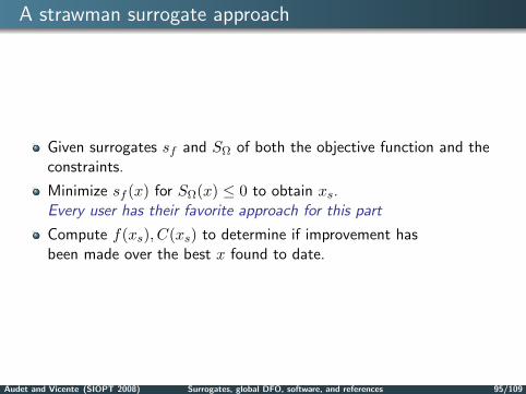

Response surface global models
Choose a space filling set of points.– say by Latin hypercube or orthogonal array sampling.
Run the expensive simulations at these sites.
Interpolate or smooth to f, C on this data.
May be able to interpolate to gradients as well – Alexandrov
Audet and Vicente (SIOPT 2008) Surrogates, global DFO, software, and references 96/109
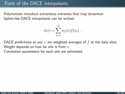
Form of the DACE interpolants
Polynomials introduce extraneous extremes that trap strawmanSpline-like DACE interpolants can be written
s(x) =d∑
i=1
wi(x)f(xi) .
DACE predictions at any x are weighted averages of f at the data sites.Weight depends on how far site is from x.Correlation parameters for each site are estimated.
Audet and Vicente (SIOPT 2008) Surrogates, global DFO, software, and references 97/109

Surrogate Management Framework
-
6
f
x1
x2
∗
∗
∗ is the incumbent solution
Audet and Vicente (SIOPT 2008) Surrogates, global DFO, software, and references 98/109

Surrogate Management Framework
-
6
f
x1
x2
∗
∗
∗ is the incumbent solution
•
Audet and Vicente (SIOPT 2008) Surrogates, global DFO, software, and references 98/109

Surrogate Management Framework
-
6
f
x1
x2
∗
∗
∗ is the incumbent solution
•
•
Audet and Vicente (SIOPT 2008) Surrogates, global DFO, software, and references 98/109

Surrogate Management Framework
-
6
f
x1
x2
∗
∗
∗ is the incumbent solution
•
•
.
.......................................
....................................
.................................
..............................
...........................
........................
.....................
....................
.........................
.....................
.............................................
.............................................
..............................................
......................................................................................................................................................................................................................................................................................
............................
........................
................................................
.................................................
. ..................... ...................... ....................... .......................... ............................ . .......................................... ....................................... .................................... ................................. .............................. ........................... ......................... ........................ ...................... ........................................................
Surrogate function
•
Trial point produced using the surrogate
Audet and Vicente (SIOPT 2008) Surrogates, global DFO, software, and references 98/109

Surrogate Management Framework
-
6
f
x1
x2
∗
∗
∗ is the incumbent solution
•
•
.
.......................................
....................................
.................................
..............................
...........................
........................
.....................
....................
.........................
.....................
.............................................
.............................................
..............................................
......................................................................................................................................................................................................................................................................................
............................
........................
................................................
.................................................
. ..................... ...................... ....................... .......................... ............................ . .......................................... ....................................... .................................... ................................. .............................. ........................... ......................... ........................ ...................... ........................................................
Surrogate function
•
•
f is evaluated at the trial point
Audet and Vicente (SIOPT 2008) Surrogates, global DFO, software, and references 98/109

Surrogate Management Framework
-
6
f
x1
x2
∗
∗
∗ is the incumbent solution
•
•
•
•
.
.......................................
....................................
.................................
..............................
...........................
........................
.....................
....................
.............................
...........................
........................................................
........................................................
.........................................................
........................................................................................................................................................................................................................................
............................
........................
................................................
.................................................
..................
....................... ........................ .......................... ............................ ............................... ................................. . ................... ................... .................... ...................... ........................
.......................... .........................
..............................................
...................... ..................... ..................... ......................
New surrogate function
the surrogate function is updated
Audet and Vicente (SIOPT 2008) Surrogates, global DFO, software, and references 98/109

Surrogate Management Framework
-
6
f
x1
x2
∗
∗
∗ is the incumbent solution
•
•
•
•
.
.......................................
....................................
.................................
..............................
...........................
........................
.....................
....................
.............................
...........................
........................................................
........................................................
.........................................................
........................................................................................................................................................................................................................................
............................
........................
................................................
.................................................
..................
....................... ........................ .......................... ............................ ............................... ................................. . ................... ................... .................... ...................... ........................
.......................... .........................
..............................................
...................... ..................... ..................... ......................
New surrogate function
the surrogate function is updatedPoll around the incumbent (order based on surrogate)
•
•
•
•
•
•
Audet and Vicente (SIOPT 2008) Surrogates, global DFO, software, and references 98/109
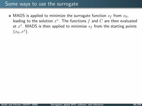
Some ways to use the surrogate
MADS is applied to minimize the surrogate function sf from x0,leading to the solution xs. The functions f and C are then evaluatedat xs. MADS is then applied to minimize sf from the starting pointsx0, x
s.At each iteration, the search and poll trial points are sorted accordingto their surrogate function values. Promising trial points areevaluated first.
At each iteration, the search step returns a list of trial points.The true functions are evaluated only at those having a goodsurrogate value.
Surrogates are updated when new information about the truth isavailable. This may be based on an interpolation model of f − sf .
Convergence analysis is not altered by the use of surrogates.
Audet and Vicente (SIOPT 2008) Surrogates, global DFO, software, and references 99/109
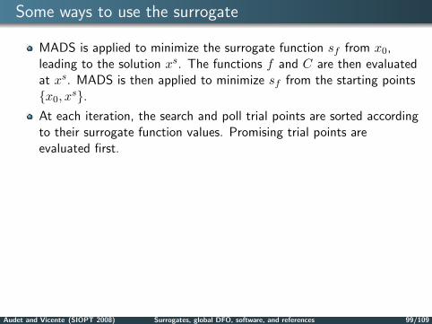

Presentation outline
1 Introduction
2 Unconstrained optimizationDirectional direct search methodsSimplicial direct search and line-search methodsInterpolation-based trust-region methods
3 Optimization under general constraintsNonsmooth optimality conditionsMads and the extreme barrier for closed constraintsFilters and progressive barrier for open constraints
4 Surrogates, global DFO, software, and referencesThe surrogate management frameworkConstrained TR interpolation-based methodsTowards global DFO optimizationSoftware and references

Constrained TR interpolation-based methods
A number of pratical trust-region SQP type methods have been proposed(see available software).
The main ideas are the following:
Use of quadratic models for the Lagrangian function.
Models for the constraints can be linear, or quadratic (especially whenfunction evaluations are expensive but leading to quadraticallyconstrained TR subproblems).
Globalization requires a merit function (typically f) or a filter.
Open constraints have no influence on the poisedness for f .
Audet and Vicente (SIOPT 2008) Surrogates, global DFO, software, and references 101/109

Constrained TR interpolation-based methods
A number of pratical trust-region SQP type methods have been proposed(see available software).
The main ideas are the following:
Use of quadratic models for the Lagrangian function.
Models for the constraints can be linear, or quadratic (especially whenfunction evaluations are expensive but leading to quadraticallyconstrained TR subproblems).
Globalization requires a merit function (typically f) or a filter.
Open constraints have no influence on the poisedness for f .
Currently, there is no (non-obvious) convergence theory developed for TRinterpolation-based methods (in the constrained case).
For example, for (i) linear or box constraints (closed) and (ii) openconstraints without derivatives, the unconstrained theory should bereasonably easy to adapt.
Audet and Vicente (SIOPT 2008) Surrogates, global DFO, software, and references 101/109
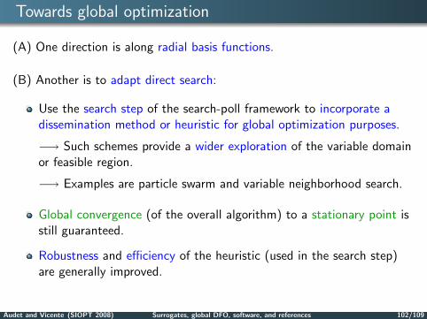
Towards global optimization
(A) One direction is along radial basis functions.
(B) Another is to adapt direct search:
Use the search step of the search-poll framework to incorporate adissemination method or heuristic for global optimization purposes.
−→ Such schemes provide a wider exploration of the variable domainor feasible region.
−→ Examples are particle swarm and variable neighborhood search.
Global convergence (of the overall algorithm) to a stationary point isstill guaranteed.
Robustness and efficiency of the heuristic (used in the search step)are generally improved.
Audet and Vicente (SIOPT 2008) Surrogates, global DFO, software, and references 102/109

Software (directional direct search)
APPSPACK: Asynchronous parallel pattern searchhttp://software.sandia.gov/appspack
NOMAD: Generalized pattern search and mesh adaptive direct searchhttp://www.gerad.ca/NOMADhttp://www.afit.edu/en/ENC/Faculty/MAbramson/NOMADm.html
Mads: Matlab’s implementation of the LtMads method – gads toolboxhttp://www.mathworks.com/products/gads
SID-PSM: Generalized pattern search guided by simplex derivativeshttp://www.mat.uc.pt/sid-psm
Audet and Vicente (SIOPT 2008) Surrogates, global DFO, software, and references 103/109

Software (direct search — others in Matlab)
Iterative Methods for Optimization: Matlab CodesHooke-Jeeves, multidirectional search, and Nelder-Mead methodshttp://www4.ncsu.edu/~ctk/matlab_darts.html
The Matrix Computation ToolboxMultidirectional search, alternating directions, and Nelder-Mead methodshttp://www.maths.manchester.ac.uk/~higham/mctoolbox
fminsearch: Matlab’s implementation of the Nelder-Mead methodhttp://www.mathworks.com/access/helpdesk/help/techdoc/ref/fminsearch.html
Audet and Vicente (SIOPT 2008) Surrogates, global DFO, software, and references 104/109

Software (trust-region interpolation based methods)
DFO: Trust-region interpolation-based methodhttp://www.coin-or.org/projects.html
UOBYQA, NEWUOA: Trust-region interpolation-based [email protected]
WEDGE: Trust-region interpolation-based methodhttp://www.ece.northwestern.edu/~nocedal/wedge.html
Audet and Vicente (SIOPT 2008) Surrogates, global DFO, software, and references 105/109

Software (others)
BOOSTERS: Trust-region interpolation-based method (based on radial basisfunctions)http://roso.epfl.ch/rodrigue/boosters.htm
CONDOR: Trust-region interpolation-based method (version of UOBYQA inparallel)http://www.applied-mathematics.net/optimization/CONDORdownload.html
Implicit Filtering: implicit filtering methodhttp://www4.ncsu.edu/~ctk/iffco.html
Audet and Vicente (SIOPT 2008) Surrogates, global DFO, software, and references 106/109
Software (Global Optimization)
PSwarm: Coordinate search and particle swarm for global optimizationhttp://www.norg.uminho.pt/aivaz/pswarm
Audet and Vicente (SIOPT 2008) Surrogates, global DFO, software, and references 107/109

Benchmarking
K. R. Fowler, J. P. Reese, C. E. Kees, J. E. Dennis Jr., C. T. Kelley,C. T. Miller, C. Audet, A. J. Booker, G. Couture, R. W. Darwin, M.W. Farthing, D. E. Finkel, J. M. Gablonsky, G. Gray, and T. G. Kolda,A comparison of derivative-free optimization methods for groundwatersupply and hydraulic capture community problems, Advances inWater Resources, 31(2): 743-757, 2008.
J. J. More and S. M. Wild, Benchmarking derivative-free optimizationalgorithms, Tech. Report ANL/MCS-P1471-1207, Mathematics andComputer Science Division, Argonne National Laboratory, USA, 2007.
Audet and Vicente (SIOPT 2008) Surrogates, global DFO, software, and references 108/109

Main references
C. Audet and J. E. Dennis, Jr., Mesh adaptive direct searchalgorithms for constrained optimization, SIAM Journal onOptimization, 17 (2006) 188–217.
A. R. Conn, K. Scheinberg, and L. N. Vicente, Introduction toDerivative-Free Optimization, MPS-SIAM Series on Optimization,SIAM, Philadelphia, to appear in 2008.
T. G. Kolda, R. M. Lewis, and V. Torczon, Optimization by directsearch: new perspectives on some classical and modern methods,SIAM Review, 45 (2003) 385–482.
Audet and Vicente (SIOPT 2008) Surrogates, global DFO, software, and references 109/109