INL/EXT-17-43438

Light Water Reactor Sustainability Program

Status of Adaptive Surrogates within the RAVEN framework

Andrea Alfonsi, Congjian Wang, Joshua Cogliati, Diego Mandelli, Cristian Rabiti

September 2017

DOE Office of Nuclear Energy

DISCLAIMER

This information was prepared as an account of work sponsored by an agency of the U.S. Government. Neither the U.S. Government nor any agency thereof, nor any of their employees, makes any warranty, expressed or implied, or assumes any legal liability or responsibility for the accuracy, completeness, or usefulness, of any information, apparatus, product, or process disclosed, or represents that its use would not infringe privately owned rights. References herein to any specific commercial product, process, or service by trade name, trade mark, manufacturer, or otherwise, does not necessarily constitute or imply its endorsement, recommendation, or favoring by the U.S. Government or any agency thereof. The views and opinions of authors expressed herein do not necessarily state or reflect those of the U.S. Government or any agency thereof.

INL/EXT-17-43438

Light Water Reactor Sustainability Program

Status of Adaptive Surrogates within the RAVEN framework

Andrea Alfonsi – INL Congjian Wang – INL Joshua Cogliati – INL Diego Mandelli – INL Cristian Rabiti – INL

September 2017

Idaho National Laboratory Idaho Falls, Idaho 83415

http://www.inl.gov/lwrs

Prepared for the U.S. Department of Energy Office of Nuclear Energy

Under DOE Idaho Operations Office Contract DE-AC07-05ID14517

iii

ABSTRACT

The RAVEN code has been under development at the Idaho National Laboratory since 2012. Its main goal is to create a multi-purpose platform for the deploying of all the capabilities needed for Probabilistic Risk Assessment, uncertainty quantification, data mining analysis and optimization studies. RAVEN has demonstrated a good level of maturity in terms of state-of-art and advanced analysis methodologies. In the past year the RAVEN code has been released as open-source project and is available to download (raven.inl.gov) free of charge.

The main subject of this report is to show the activities that have been recently accomplished with respect the adaptive surrogate modeling:

• Implementation of the metric system for the assessment of surrogate model validity

• Implementation of cross-validation techniques for the global assessment of surrogate models

• Implementation of an automatic infrastructure for switching between a high-fidelity model (e.g. physical code) and a surrogate or set of surrogates

• Implementation of a scheme for automatic optimization of surrogate model parameters.

The aim of this document is to report the status of the development of methods, within the RAVEN framework, to assess the validity of the predictive capabilities of surrogate models. Indeed, after the construction of a surrogate tight to a certain physical model, it is crucial to assess the goodness of its representation, in order to be confident with its prediction. A cross-validation technique has been employed. This report will highlight the implementation details and proof of its correct implementation by an application example. The implementation of a way to assess the predictive capabilities of a surrogate allowed the construction of a RAVEN new entity named “HybridModel” that is aimed to switch between a high-fidelity code and its linked surrogate. In addition, leveraging the optimization algorithms that have been implemented in RAVEN in the last fiscal year, a new scheme has been developed for automatic tuning of the surrogates’ parameters (e.g. penalty factors in support vector machines).

iv

CONTENTS

ABSTRACT ................................................................................................................................................. iii

FIGURES ....................................................................................................................................................... v

TABLES ....................................................................................................................................................... vi

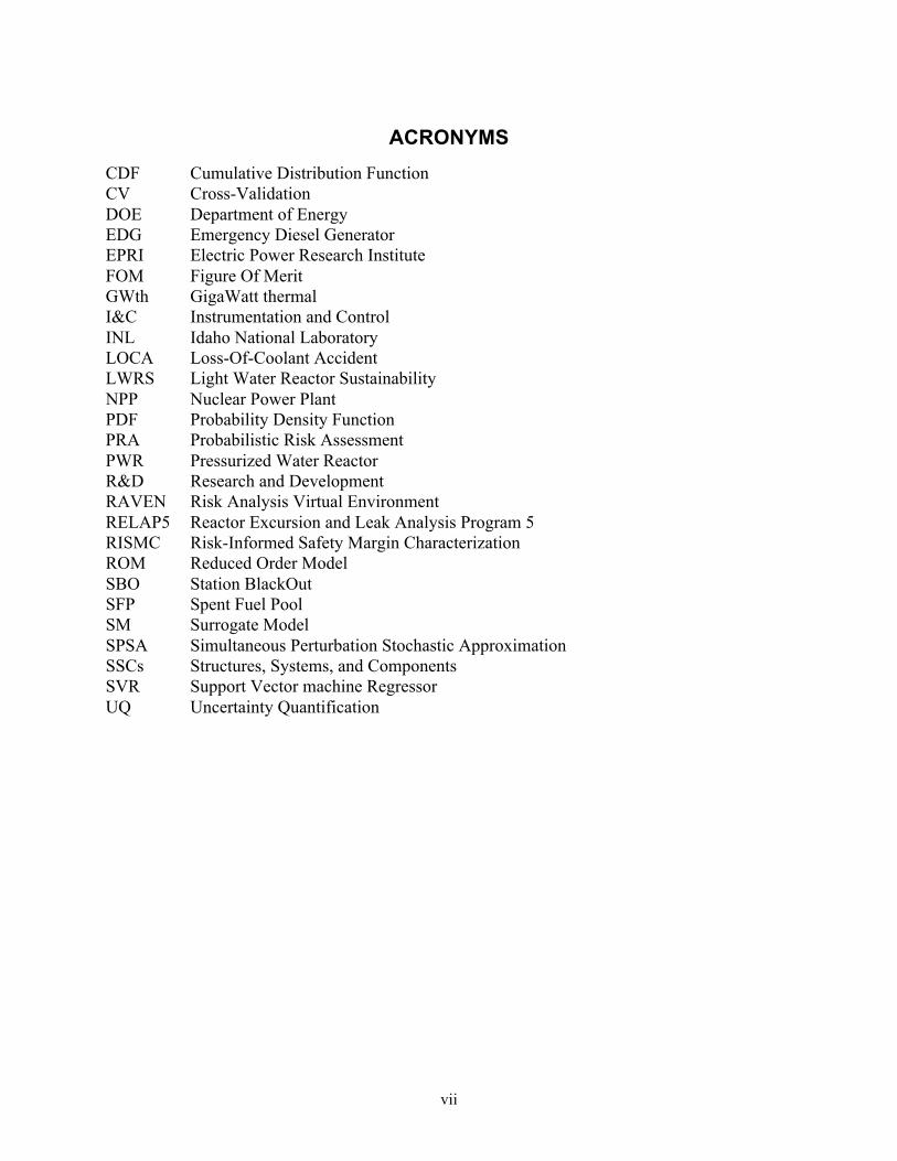
ACRONYMS .............................................................................................................................................. vii

1. INTRODUCTION ............................................................................................................................... 1

2. METRIC SYSTEM ............................................................................................................................. 32.1 Distance and Similarity metrics ................................................................................................ 3

2.1.1 Distance metrics ........................................................................................................... 32.1.2 Similarity metrics ......................................................................................................... 4

2.2 Probabilistic metrics .................................................................................................................. 52.3 Scoring metrics ......................................................................................................................... 62.4 Metrics Post-Processor .............................................................................................................. 7

3. CROSS VALIDATION ...................................................................................................................... 93.1 Cross Validation for assessing surrogate modeling prediction capabilities ............................ 103.2 RAVEN implementation ......................................................................................................... 11

4. SURROGATE MODELS PARAMETER OPTIMIZATION ........................................................... 13

5. AUTOMATIC SELECTION OF HIGH-FIDELITY AND SURROGATE MODELS: HYBRID MODEL ENTITY ............................................................................................................. 16

6. APPLICATION EXAMPLES ........................................................................................................... 196.1 Description of the simulated scenario: SBO of a PWR .......................................................... 19

6.1.1 Initiating Event .......................................................................................................... 206.1.2 Accident progression ................................................................................................. 206.1.3 PWR Model ............................................................................................................... 206.1.4 Stochastic Model ........................................................................................................ 21

6.2 Cross Validation for trained Surrogate Model ........................................................................ 226.2.1 Cross-Validation for a constructed surrogate model ................................................. 22

6.3 Optimization of Surrogate Model Parameters ........................................................................ 256.4 Hybrid Model for Probabilistic Risk Assessment analysis ..................................................... 26

7. conclusions ........................................................................................................................................ 28

8. REFERENCES .................................................................................................................................. 29

v

FIGURES Figure 1 - Metric post-processor functional scheme ......................................................................................8Figure 2 - Cross-Validation dataset partitioning example .............................................................................9Figure 3 – Functional scheme for the cross-validation postprocessor in RAVEN. .....................................12Figure 4 - SVR prediction performance varying C and gamma parameters. ..............................................13Figure 5 - RAVEN optimization workflow .................................................................................................14Figure 6 - Optimization scheme for Surrogate Model parameter selection. ................................................14Figure 7 - RAVEN automatic model selection scheme. ..............................................................................18Figure 8 - Generic scheme of the PWR system. ..........................................................................................19Figure 9 - PWR nodalization .......................................................................................................................21Figure 10 - Temperature profile for the Pump Controller. .........................................................................22Figure 11 - Explained variance score as function of # samples. .................................................................23Figure 12 - Mean absolute error score as function of # samples. ................................................................24Figure 13 - Mean squared error score as function of # samples. .................................................................24Figure 14 - Optimization trajectory. ............................................................................................................26

vi

TABLES Table 1 - SVR SM settings. .........................................................................................................................23Table 2 - SVR SM parameters for the optimization. ...................................................................................25Table 3 – Optimization settings. ..................................................................................................................25Table 4 CV parameters. ...............................................................................................................................26Table 5 HybridModel statistical moments. ..................................................................................................27Table 6 RELAP5-3D statistical moments ....................................................................................................27

vii

ACRONYMS

CDF Cumulative Distribution Function CV Cross-Validation DOE Department of Energy EDG Emergency Diesel Generator EPRI Electric Power Research Institute FOM Figure Of Merit GWth GigaWatt thermal I&C Instrumentation and Control INL Idaho National Laboratory LOCA Loss-Of-Coolant Accident LWRS Light Water Reactor Sustainability NPP Nuclear Power Plant PDF Probability Density Function PRA Probabilistic Risk Assessment PWR Pressurized Water Reactor R&D Research and Development RAVEN Risk Analysis Virtual Environment RELAP5 Reactor Excursion and Leak Analysis Program 5 RISMC Risk-Informed Safety Margin Characterization ROM Reduced Order Model SBO Station BlackOut SFP Spent Fuel Pool SM Surrogate Model SPSA Simultaneous Perturbation Stochastic Approximation SSCs Structures, Systems, and Components SVR Support Vector machine Regressor UQ Uncertainty Quantification

1

Status of Adaptive Surrogates within the RAVEN framework

1. INTRODUCTION

The overall goal of the Risk Analysis in a Virtual ENvironment (RAVEN) software is to understand the probabilistic behavior/response of complex systems. In particular RAVEN is focused on risk analysis. The capability to predict the likelihood that the system under consideration will end in a particular region of the output space, which is the base of the risk analysis, is already an available feature of the RAVEN code (i.e., the “limit surface” approach). Those types of analyses rely on the availability of probability distributions and sampling strategies, according to which the input space of the probabilistic systems are explored, and statistical post processors used to understand the dispersion of the system response.

In the past years RAVEN capabilities were extended to provide the tools to the engineers to better understand the reasons/drivers (the main patterns) of the system responses by adding advanced sampling strategies (e.g. hybrid dynamic event tree and adaptive hybrid dynamic even tree) [1,2], advanced static and time-dependent data mining capabilities (e.g. clustering, principal component analysis, manifold learning) [3], infrastructure to connect multiple reduced order model (able to reproduce scalar and history-type figure of merits) in order to create ensemble of models, advanced topological space decomposition, etc.

While these added capabilities showed remarkable outcomes in terms of analysis workflows, it was clear that some additional enhancements were needed in order to accelerate (in terms of computational times) the analysis process providing ways to associate to the acceleration schemes a way to assess the “confidence” associated to the final outcomes and, eventually, to use this “confidence” metric to be able to choose among different models with different level of fidelity.

This is the motivation for why multiple parallel activities have been performed this year, all of them oriented to better performing surrogate modelling:

• Implementation of the metric system for the assessment of surrogate model validity: In order to compare different datasets, a system of metrics have been implemented. Indeed, in order to assess “how close” two datasets are, a scoring method (i.e. a method that is able to “measure” the “distance” between datasets) is a key component.

• Implementation of cross-validation techniques for the global assessment of surrogate models: After the construction of a surrogate tied to a certain physical model, it is crucial to assess the goodness of its representation, in order to be confident with its prediction. A promising and largely used technique for assessing the global validity of a surrogate model is called cross-validation. This method is a statistical methodology that partitions the training space and tests the surrogate against the real data. The “validity” is assessed comparing the real data with the predicted evaluations using ad-hoc metrics. It is clear how the implementation and development of the Metric system was propaedeutic to the development of a robust and

2

agnostic cross-validation module. This development in RAVEN allows analysts to build complex models and have a method to determine the overall fidelity of those.

• Implementation of a scheme for automatic optimization of surrogate model parameters: The choice of a surrogate model (i.e. the particular algorithm, the settings, etc.) is always challenging if the user is not completely familiar with the mathematical formulations of the surrogates of choice and the behavior, under combined uncertainties, of the system that he wants to surrogate (e.g. non-linear behavior, presence of discontinuities, etc.). In order to facilitate the settings of the surrogates in RAVEN, an automatic optimization scheme has been developed to choose the surrogate parameters and settings in order to maximize the global validity of the model giving a fixed training set.

• Implementation of an automatic infrastructure for switching between a high-fidelity model (e.g. physical code) and a surrogate or set of surrogates: The final activity that has been performed this year is about the construction of an infrastructure to automatically switch between a set of surrogate models and a high-fidelity code. The switching strategy is based on local validation metrics that are able to provide an assessment on the goodness of the prediction made by a surrogate model. This decision metric decides if the surrogate is good enough for a certain realization or if the high-fidelity model needs to be used.

The report is organized as follows: 1) Section 2 reports the development of the metric system within RAVEN.

2) Section 3 shows cross-validation techniques used to testify the convergence of surrogate models.

3) Section 4 is about the development of the automatic optimization of surrogate model parameters

4) Section 5 documents the implementation of the automatic infrastructure for surrogate/high-fidelity models switching.

5) Section 6 shows application results on a PWR SBO case. 6) Section 7 concludes the report, highlighting the future development directions.

3

2. METRIC SYSTEM In data analysis, in general, and model validation, in particular, the ability to compare different

datasets is crucial to get a measurement of “how close” two (or more) datasets are. In order to fulfill this need, a new module has been developed in RAVEN: The Metric system. This entity is in charge of collecting all the algorithms that are able to assess the similarity/dissimilarity of datasets.

Multiple distance/scoring metrics has been implemented in the system in order to cover all the possible cases where datasets need to be compared:

- Distance and Similarity metrics, mostly aimed to deliver a set of methods to compare different data sets in order to answer to the questions “how close?” (Distance) or “how similar?” (Similarity) the two datasets are

- Probabilistic metrics, mainly aimed to provide a set of algorithms to compare model evaluations and experiments (e.g. code validation) in a probabilistic environment

- Scoring metrics, principally envisioned to fulfill the needs to assess how good regression models are (e.g. surrogate model validation)

Independently of the envisioned scope of these metrics (e.g. code validation, surrogate model validation, etc.), the user is able to use any metric in any of the user cases reported in the bullets above.

In the following sections, the three main classes of metrics are briefly reported.

2.1 Distance and Similarity metrics In the following sections, the distance and similarity metrics are reported. Both types of metrics are

widely used for assessing the similarity/dissimilarity of datasets. 2.1.1 Distance metrics

A distance metric is a function that defines a distance between each pair of elements of a set:

𝑑: 𝑋×𝑋 → 0,∞) where 0,∞) is the set of non-negative real numbers. A distance metric satisfies the following

conditions:

- separation axiom: 𝑑 𝑢, 𝑣 ≥ 0

- identity: 𝑑 𝑢, 𝑣 = 0 ⟺ 𝑢 = 𝑣

- symmetry: 𝑑 𝑢, 𝑣 = 𝑑 𝑣, 𝑢

- triangle inequality: 𝑑 𝑢, 𝑘 ≤ 𝑑 𝑢, 𝑣 + 𝑑 𝑣, 𝑘 As inferable from above, these metrics are conceived to measure the distance between data sets.

During this FY, the following distance metrics have been made available: - Manhattan distance metric (L1):

𝑑(𝒖, 𝒗) = 𝑢6 − 𝑣6

8

69:

- Euclidian distance metric (L2):

4

𝑑(𝒖, 𝒗) = 𝑢6 − 𝑣6 ;

8

69:

- Minkowski distance metric (Lp):

𝑑(𝒖, 𝒗) = 𝑢6 − 𝑣6 <

8

69:

=

- Canberra distance metric:

𝑑(𝒖, 𝒗) = 𝑢6 − 𝑣6𝑢6 + 𝑣6

8

69:

- Bray-Curtis distance metric:

𝑑(𝒖, 𝒗) = 𝑢6 − 𝑣6

8

69:

𝑢6 + 𝑣6

8

69:

- Correlation distance metric:

𝑑 𝒖, 𝒗 = 1 −(𝒖 − 𝑢) ∙ (𝒗 − 𝑣)𝒖 − 𝑢 ; 𝒗 − 𝑣 ;

where 𝑢 and 𝑣 are the means of the elements of 𝒖 and 𝒗 respectively

- Cosine distance metric:

𝑑 𝒖, 𝒗 = 1 −𝒖 ∙ 𝒗𝒖 ; 𝒗 ;

2.1.2 Similarity metrics A similarity metric (or measure) is a real-valued function that quantifies the similarity among

datasets. In a simplistic view, a similarity metric can be seen as the inverse of a distance metric; intuitively, higher is its score more similar the datasets are.

During this FY, the following similarity metrics have been delivered in the RAVEN code: - Cosine similarity metric:

𝑘(𝒖, 𝒗) =𝒖𝒗𝑻

𝒖 𝒗

The cosine similarity is the L2-normalized dot product of the vectors 𝒖 and 𝒗. It is named “cosine” similarity since Euclidean (L2) normalization projects the vectors onto the unit sphere, and their dot product is then the cosine of the angle between the points denoted by the vectors.

- Polynomial similarity metric:

𝑘(𝒖, 𝒗) = (𝛾𝒖𝒗𝑻 + 𝑐C)D

5

The polynomial similarity computes the degree-d polynomial kernel between two vectors, where 𝑐C is known as intercept and 𝛾 is the slope. The polynomial kernel represents the similarity between two datasets.

- Sigmoid similarity metric:

𝑘(𝒖, 𝒗) = 𝑡𝑎𝑛ℎ(𝛾𝒖𝒗𝑻 + 𝑐C) The sigmoid similarity computes the sigmoid kernel between two vectors. The sigmoid

kernel is also known as hyperbolic tangent, where 𝑐C is known as intercept and 𝛾 is the slope.

- Radial Basis Function similarity metric:

𝑘(𝒖, 𝒗) = 𝑒𝑥𝑝(−𝛾 𝒖 − 𝒗 ;) where 𝛾 is the slope.

- Laplacian similarity metric:

𝑘(𝒖, 𝒗) = 𝑒𝑥𝑝(−𝛾 𝒖 − 𝒗 ) where 𝒖 − 𝒗 is the L1 distance metric and 𝛾 is the slope.

- Chi-squared similarity metric:

𝑘(𝒖, 𝒗) = 𝑒𝑥𝑝 −𝛾(𝑢6 − 𝑣6);

𝑢6 + 𝑣66

where 𝛾 is the slope.

2.2 Probabilistic metrics

The probabilistic metrics are measurement of the distance of datasets in a probabilistic sense. They assume that the data are part of a statistical population and, consequentially, involve the probability reconstruction of the datasets to be compared.

The following probabilistic metrics have been made available in RAVEN (and usable for any dataset):

- CDF area metric (Minkowski L1 metric):

𝑘𝑝(𝒖, 𝒗) = 𝐶𝐷𝐹 𝑢 − 𝐶𝐷𝐹(𝑣)OP

QP

This metric computes the area contained between the two CDFs generated based on the 𝒖 and 𝒗 vectors.

- PDF area metric:

𝑘𝑝(𝒖, 𝒗) = min 𝑃𝐷𝐹 𝑢 , 𝑃𝐷𝐹(𝑣)OP

QP

6

2.3 Scoring metrics The scoring metrics are measurements that are aimed, alike the distance ones, to assess the distance

between datasets. They are generally statistical metrics that aim to provide the distance in terms of “error”.

In RAVEN, the following ones have been considered: - Discrete (or Boolean) datasets:

o Accuracy score:

If 𝑣V and 𝑢6 are the values of the 𝑖 − 𝑡ℎ points in the datasets𝒗and 𝒖 respectively, then the fraction of matches over 𝑛XYZ<[\X is defined as:

𝑎𝑐𝑐𝑢𝑟𝑎𝑐𝑦 𝒖, 𝒗 = 1

𝑛XYZ<[\X1(

8_`a=bc_

69:

𝑣V = 𝑢6)

where 1(𝑥) is the indicator function1. o Precision score:

The precision score is the ratio 𝑡𝑝/(𝑡𝑝 + 𝑓𝑝)where 𝑡𝑝 is the number of true positives and 𝑓𝑝 is the number of false positives. In classification, the precision is the ability of the classifier not to label as positive a sample that is negative.

o Recall score:

The recall score is the ratio 𝑡𝑝/(𝑡𝑝 + 𝑓𝑛)where 𝑡𝑝 is the number of true positives and 𝑓𝑛 the number of false negatives. In classification, the recall is the ability of the classifier to find all the positive samples.

o Average precision score: It is a score that is based on the computation of the average precision from predictions. The score corresponds to the area under the precision-recall curve.

o Balanced F-score:

The balanced F-score can be represented as a weighted average of the precision and recall, where an F1 score reaches its best value at 1 and worst score at 0. The relative contribution of precision and recall to the F1 score are equal. The formula for the F1 score is:

𝐹1 = 2 ∗(𝑝𝑟𝑒𝑐𝑖𝑠𝑖𝑜𝑛 ∗ 𝑟𝑒𝑐𝑎𝑙𝑙)(𝑝𝑟𝑒𝑐𝑖𝑠𝑖𝑜𝑛 + 𝑟𝑒𝑐𝑎𝑙𝑙)

o Cross entropy loss score: This score is based on the loss function used in (multinomial) logistic regression and extensions of it such as neural networks, defined as the negative log-likelihood of the true labels given a probabilistic classifier’s predictions. For a single sample with true label 𝑦𝑡𝑖𝑛{0,1} and estimated probability 𝑦𝑝 that 𝑦𝑡 = 1, the log loss is:

1 Function defined on a set X that indicates membership of an element in a subset A of X, having the value 1 for all elements of A and

the value 0 for all elements of X not in A

7

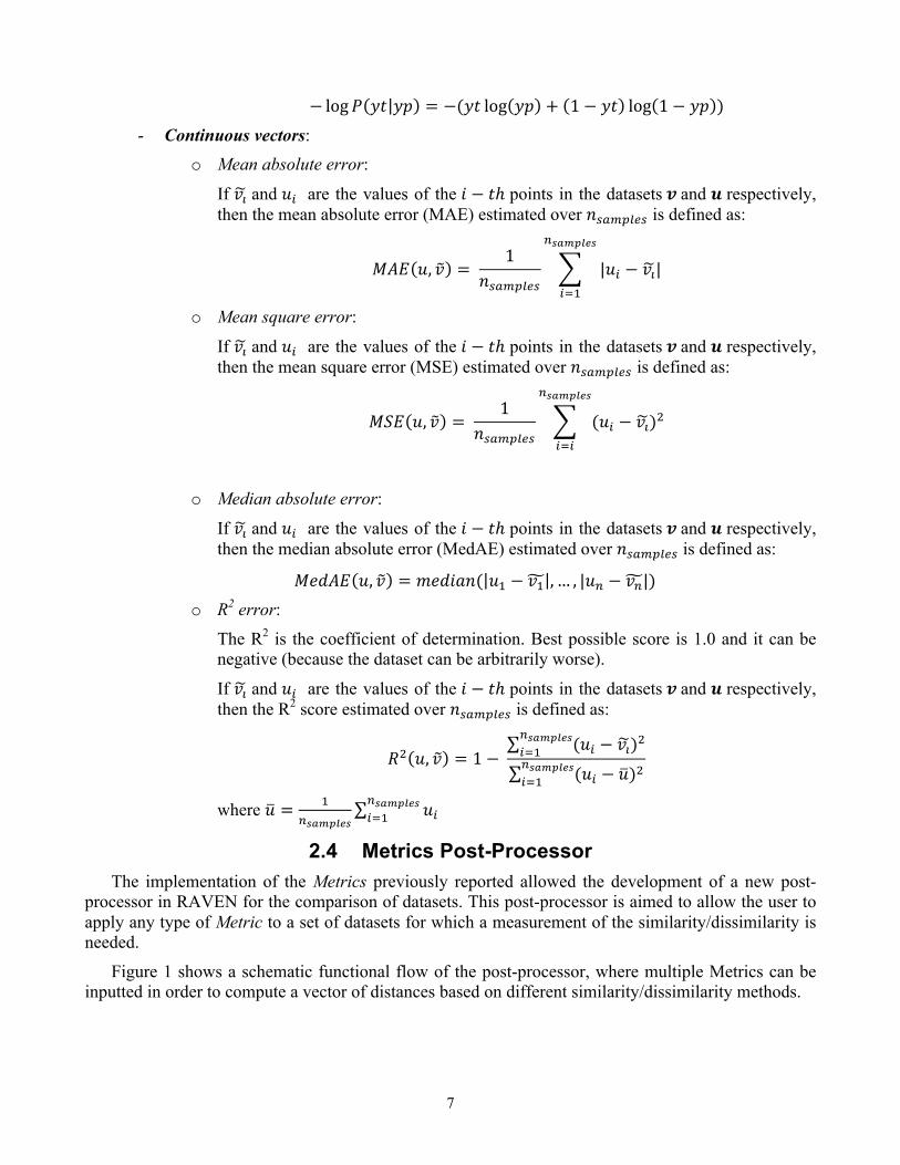
− log𝑃 𝑦𝑡 𝑦𝑝 = −(𝑦𝑡 log 𝑦𝑝 + 1 − 𝑦𝑡 log 1 − 𝑦𝑝 ) - Continuous vectors:

o Mean absolute error:

If 𝑣V and 𝑢6 are the values of the 𝑖 − 𝑡ℎ points in the datasets𝒗and 𝒖 respectively, then the mean absolute error (MAE) estimated over 𝑛XYZ<[\X is defined as:

𝑀𝐴𝐸 𝑢, 𝑣 = 1

𝑛XYZ<[\X|𝑢6 − 𝑣V|

8_`a=bc_

69:

o Mean square error:

If 𝑣V and 𝑢6 are the values of the 𝑖 − 𝑡ℎ points in the datasets𝒗and 𝒖 respectively, then the mean square error (MSE) estimated over 𝑛XYZ<[\X is defined as:

𝑀𝑆𝐸 𝑢, 𝑣 = 1

𝑛XYZ<[\X(𝑢6 − 𝑣V);

8_`a=bc_

696

o Median absolute error:

If 𝑣V and 𝑢6 are the values of the 𝑖 − 𝑡ℎ points in the datasets𝒗and 𝒖 respectively, then the median absolute error (MedAE) estimated over 𝑛XYZ<[\X is defined as:

𝑀𝑒𝑑𝐴𝐸 𝑢, 𝑣 = 𝑚𝑒𝑑𝑖𝑎𝑛( 𝑢: − 𝑣: , … , |𝑢8 − 𝑣8|) o R2 error:

The R2 is the coefficient of determination. Best possible score is 1.0 and it can be negative (because the dataset can be arbitrarily worse).

If 𝑣V and 𝑢6 are the values of the 𝑖 − 𝑡ℎ points in the datasets𝒗and 𝒖 respectively, then the R2 score estimated over 𝑛XYZ<[\X is defined as:

𝑅; 𝑢, 𝑣 = 1 −(𝑢6 − 𝑣V);

8_`a=bc_69:

(𝑢6 − 𝑢);8_`a=bc_69:

where 𝑢 = :8_`a=bc_

𝑢68_`a=bc_69:

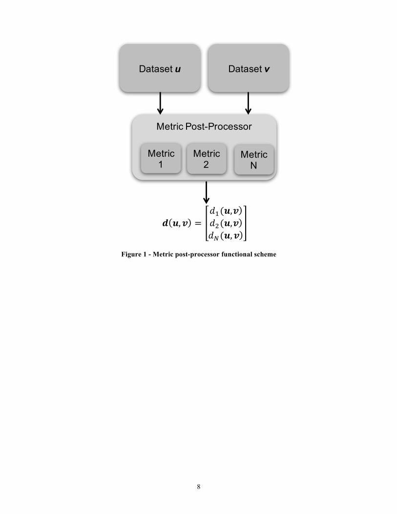
2.4 Metrics Post-Processor The implementation of the Metrics previously reported allowed the development of a new post-

processor in RAVEN for the comparison of datasets. This post-processor is aimed to allow the user to apply any type of Metric to a set of datasets for which a measurement of the similarity/dissimilarity is needed.

Figure 1 shows a schematic functional flow of the post-processor, where multiple Metrics can be inputted in order to compute a vector of distances based on different similarity/dissimilarity methods.

8

Figure 1 - Metric post-processor functional scheme

Dataset u Dataset v

Metric Post-Processor

Metric 1

Metric 2

Metric N

! ",$ =&'(",$)&*(",$)&+(", $)

9

3. CROSS VALIDATION An important path in RAVEN analysis workflow is represented by the heavy usage of Surrogate

Models (a.k.a. Reduced Order Model - ROM). A Surrogate Model is a mathematical model of fast solution trained to predict a response of interest of a physical system. The training process is performed by “sampling” the response of a physical model with respect to variations of parameters that are subject to probabilistic or parametric behavior. These samples are fed into the ROM that tunes itself to replicate those results.

In the RAVEN case the SM is constructed to emulate a numerical representation of a physical system. Indeed, the physical model is often too expensive to be used for propagating the uncertainties in the whole input space.

In RAVEN, several SMs are available: Support Vector Machine, Neighbors-based, multi-class models, Quadratic Discriminants, etc. All these SMs have been imported via an Application Programming Interface (API) within the scikit-learn library [4] and few have been also specifically developed (e.g. Polynomial Chaos, N-Dimensional Spline regressors, topology-based regressors, etc.).

At the begin of FY17 the RAVEN user did not have any easy way to assess the validity of a constructed SM, since no statistical methodologies were available to define “how good” the prediction capability of a SM was. This aspect represented a large limitation on the usage of SMs for uncertainty quantification and probabilistic risk assessment, since the user was not able to fully “trust” the response of a SM, overall when the response of the system (in terms of trends) was not known. The development under RISMC for the RAVEN code has been focused on addressing this limitation, defining and implementing “validation” techniques for SM construction and usage.

In order to tackle this problem, the RAVEN team decided to implement a black-box approach that could be used for all the SMs currently available: cross-validation. As detailed in next section, the cross-validation is a statistical method of comparing and evaluating the validity of learning algorithms (i.e. classification and regression algorithms) in modeling the response of a physical system. Through this methodology it is possible to assess the validity of the regression/classification algorithms in emulating the response of the system. In the following section, the concept of cross-validation is detailed and its implementation in RAVEN is reported.

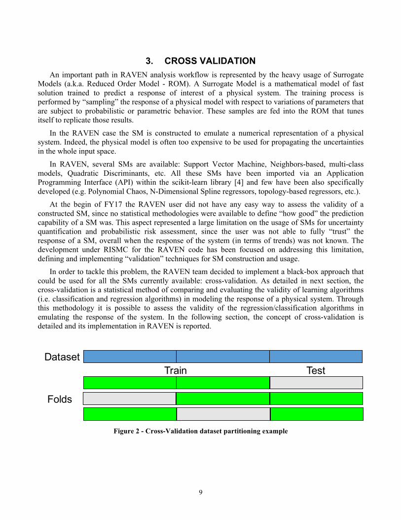
Figure 2 - Cross-Validation dataset partitioning example

Train TestDataset

Folds

10

3.1 Cross Validation for assessing surrogate modeling prediction capabilities

As previously mentioned, the approach that has been chosen for providing initial SM validation capabilities in RAVEN is based on cross-validation. Cross-validation is a statistical method of evaluating and comparing learning algorithms by dividing data into two portions: one used to “train” a surrogate model (building the surrogate model) and the other used to validate the model, based on specific distance/similarity/scoring metrics. In typical cross-validation, the training and validation sets must crossover in successive rounds such that each data point has a chance of being validated against the various sets. The basic form of cross-validation is k-fold cross-validation. Other forms of cross-validation are special cases of k-fold cross-validation or involve repeated rounds of k-fold cross-validation. Figure 2 shows an example on how the “training” dataset is partitioned in multiple folds in order to employ the cross-validation technique.

Cross-validation is used to evaluate or compare learning algorithms as follows: in each iteration, one or more learning algorithms use k folds of data to learn one or more models, and subsequently the learned models are asked to make predictions about the data in the validation fold. The performance of each learning algorithm on each fold can be tracked using some pre-determined scoring/distance metric (see Sect. 2). Upon completion, k samples of the performance metric will be available for each algorithm. Different methodologies such as averaging can be used to obtain an aggregate measure from these samples, or these samples can be used in a statistical hypothesis test to show that one algorithm is superior to another.

As highlighted in [5], there are two possible goals in cross-validation:

• To estimate performance of the learned model from available data using one algorithm. In other words, to gauge the generalizability of an algorithm

• To compare the performance of two or more different algorithms and find out the best algorithm for the available data, or alternatively to compare the performance of two or more variants of a parameterized model.

The above two goals are highly related, since the second goal is automatically achieved if one knows the accurate estimates of performance. Given a sample of N data instances and a learning algorithm A, the average cross-validated accuracy of A on these N instances may be taken as an estimate for the accuracy of A on unseen data when A is trained on all N instances. Alternatively, if the end goal is to compare two learning algorithms, the performance samples obtained through cross-validation can be used to perform two-sample statistical hypothesis tests, comparing a pair of learning algorithms.

Concerning these two goals, various procedures are available:

• Re-substitution Validation: In re-substitution validation, the model is learned from all the available data and then tested on the same set of data. This validation process uses all the available data but suffers seriously from over-fitting. That is, the algorithm might perform well on the available data yet poorly on future unseen test data.

• Hold-Out Validation: To avoid over-fitting, an independent test set is preferred. A natural approach is to split the available data into two non-overlapped parts: one for training and the other for testing. The

11

test data is held out and not looked at during training. Holdout validation avoids the overlap between training data and test data, yielding a more accurate estimate for the generalization performance of the algorithm. The downside is that this procedure does not use all the available data and the results are highly dependent on the choice for the training/test split. To deal with these challenges and utilize the available data to the max, k-fold cross-validation is used.

• K-Fold Cross-Validation: In k-fold cross-validation the data is first partitioned into k-equally (or nearly equally) sized segments or olds. Subsequently k iterations of training and validation are performed such that within each iteration a different fold of the data is held-out for validation while the remaining k-1 folds are used for learning. Data is commonly stratified prior to being split into k folds. Stratification is the process of rearranging the data as to ensure each fold is a good representative of the whole. For example, in a binary classification problem where each class comprises 50% of the data, it is best to arrange the data such that in every fold, each class comprises around half the instances.

• Leave-One-Out Cross-Validation: Leave-one-out cross-validation (LOOCV) is a special case of k-fold cross-validation where k equals the number of instances in the data. In other words, in each iteration nearly all the data except for a single observation are used for training and the model is tested on that single observation. An accuracy estimate obtained using LOOCV is known to be almost unbiased but it has high variance, leading to unreliable estimates [6]. It is still widely used when the available data are very rare, especially in bioinformatics where only dozens of data samples are available.

• Repeated K-Fold Cross-Validation: To obtain reliable performance estimation or comparison, large number of estimates is always preferred. In k-fold cross-validation, only k estimates are obtained. A commonly used method to increase the number of estimates is to run k-fold cross-validation multiple times. The data is reshuffled and re-stratified before each round.

3.2 RAVEN implementation The implementation of the cross-validation technique involved the development of a new post-

processor able to leverage the functionalities introduced by the Metric entity previously documented. Indeed, as inferable from the previous section, the final step of the cross-validation statistical method is the comparison of the outcomes, predicted by the SM, on multiple test datasets with the true values of the “high-fidelity” model, after partitioning the training data.

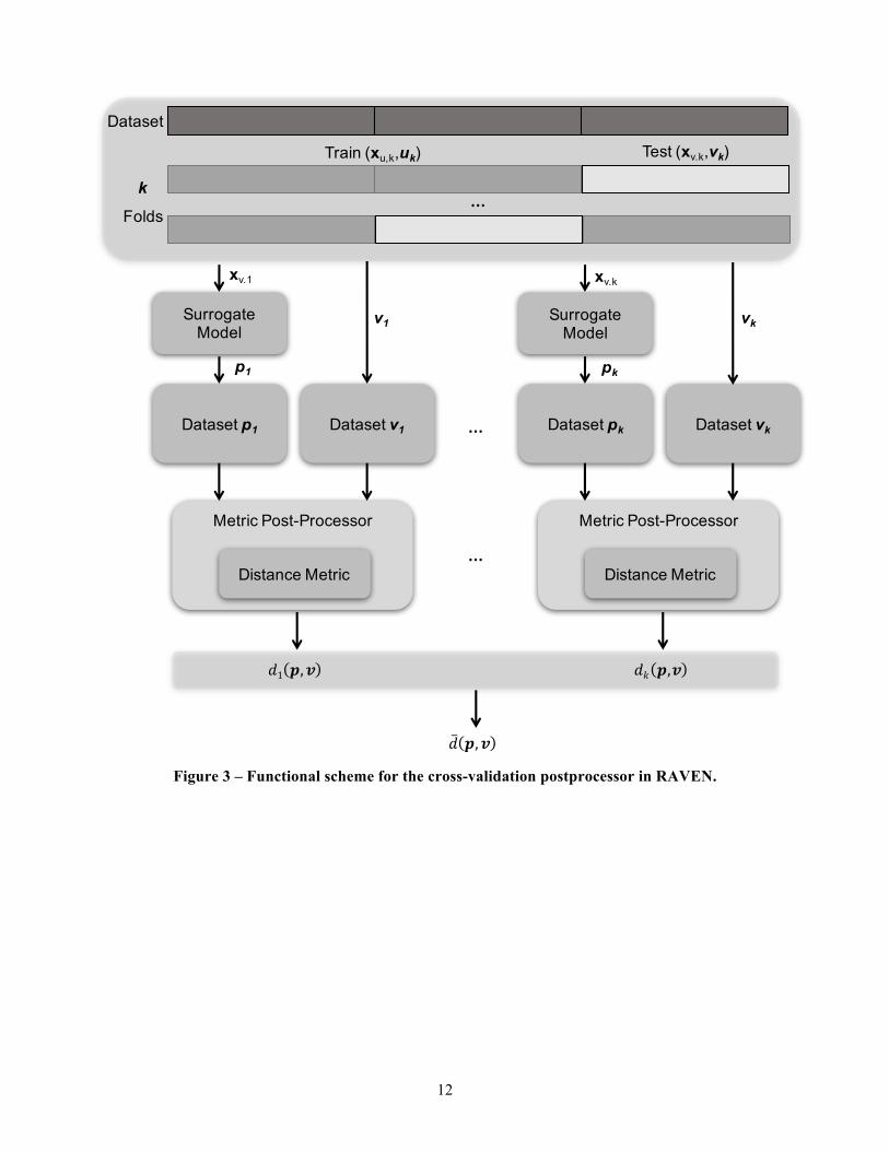
Figure 3 shows a functional scheme of the cross-validation post-processor. The training data (contained in RAVEN data storage objects) is partitioned based on any of the strategies listed in previous section. Part of the training data (xu,k ,uk) are used to construct the surrogate model and the remaining data are used for testing (xv,k ,vk). The post-processor used the newly constructed surrogate model to predict the outcomes of the test dataset (xv,k), obtaining the vector of predicted values pk. The predicted and true values are then compared based on any distance/similarity metric obtaining a distance Figure of Merit (FOM) dk(p,v). The post-processor repeats the process for all the folds k and the resulting distances are then averaged.

12

Figure 3 – Functional scheme for the cross-validation postprocessor in RAVEN.

Dataset p1 Dataset v1

Metric Post-Processor

Distance Metric

!1 #, %

Dataset pk Dataset vk

Metric Post-Processor

Distance Metric

!& #,%

…

…

Train (xu,k,uk) Test (xv.k,vk)

Dataset

k

Folds…

!̅ #, %

Surrogate Model

Surrogate Model

p1 pk

xv.1 xv.k

v1 vk

13

4. SURROGATE MODELS PARAMETER OPTIMIZATION The choice of a surrogate model (i.e. the particular algorithm, the settings, etc.) is always

challenging if the user is not completely familiar with the mathematical formulations of the surrogates of choice and the behavior, under combined uncertainties, of the system that he wants to surrogate (e.g. non-linear behavior, presence of discontinuities, etc.).

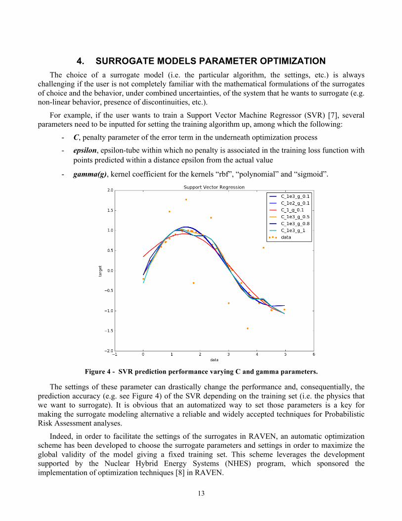
For example, if the user wants to train a Support Vector Machine Regressor (SVR) [7], several parameters need to be inputted for setting the training algorithm up, among which the following:

- C, penalty parameter of the error term in the underneath optimization process - epsilon, epsilon-tube within which no penalty is associated in the training loss function with

points predicted within a distance epsilon from the actual value

- gamma(g), kernel coefficient for the kernels “rbf”, “polynomial” and “sigmoid”.

Figure 4 - SVR prediction performance varying C and gamma parameters.

The settings of these parameter can drastically change the performance and, consequentially, the prediction accuracy (e.g. see Figure 4) of the SVR depending on the training set (i.e. the physics that we want to surrogate). It is obvious that an automatized way to set those parameters is a key for making the surrogate modeling alternative a reliable and widely accepted techniques for Probabilistic Risk Assessment analyses.

Indeed, in order to facilitate the settings of the surrogates in RAVEN, an automatic optimization scheme has been developed to choose the surrogate parameters and settings in order to maximize the global validity of the model giving a fixed training set. This scheme leverages the development supported by the Nuclear Hybrid Energy Systems (NHES) program, which sponsored the implementation of optimization techniques [8] in RAVEN.

14

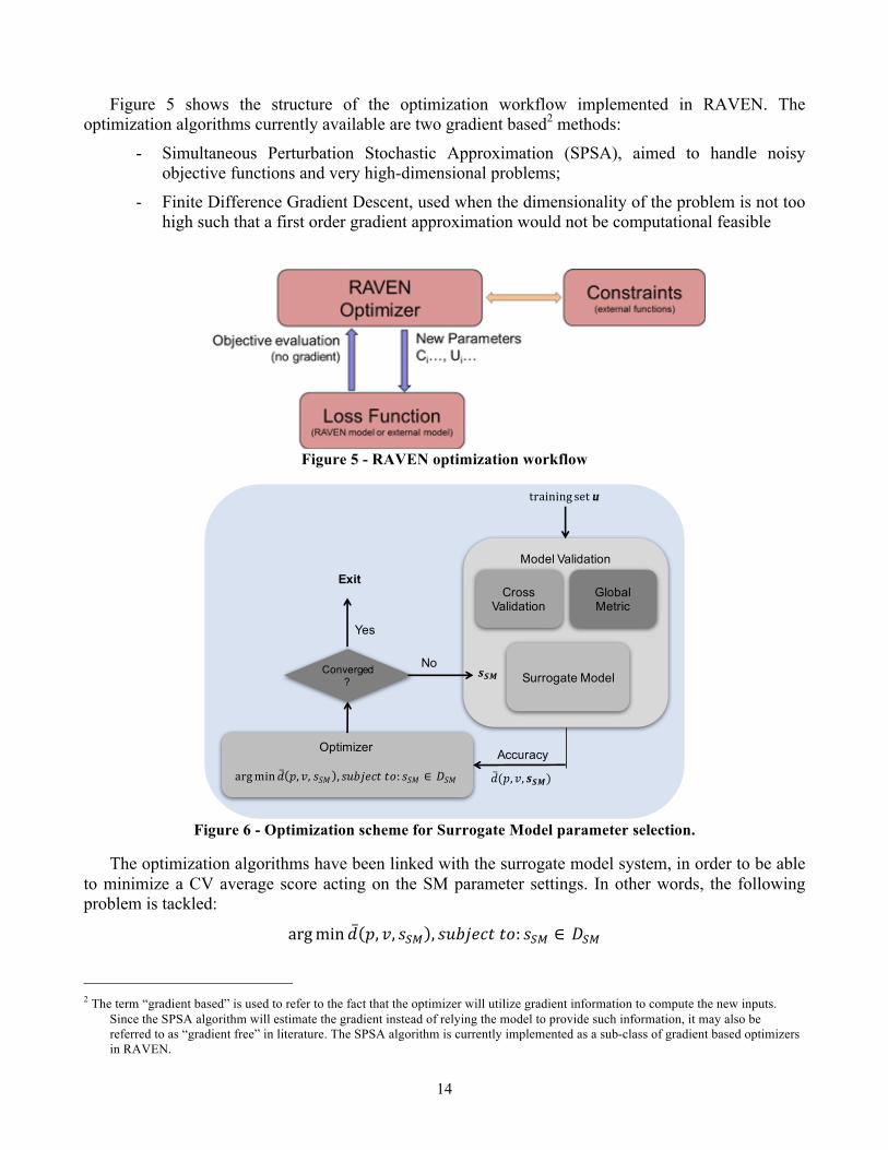
Figure 5 shows the structure of the optimization workflow implemented in RAVEN. The optimization algorithms currently available are two gradient based2 methods:

- Simultaneous Perturbation Stochastic Approximation (SPSA), aimed to handle noisy objective functions and very high-dimensional problems;

- Finite Difference Gradient Descent, used when the dimensionality of the problem is not too high such that a first order gradient approximation would not be computational feasible

Figure 5 - RAVEN optimization workflow

Figure 6 - Optimization scheme for Surrogate Model parameter selection.

The optimization algorithms have been linked with the surrogate model system, in order to be able to minimize a CV average score acting on the SM parameter settings. In other words, the following problem is tackled:

argmin 𝑑 𝑝, 𝑣, 𝑠z{ , 𝑠𝑢𝑏𝑗𝑒𝑐𝑡𝑡𝑜: 𝑠z{ ∈ 𝐷z{ 2 The term “gradient based” is used to refer to the fact that the optimizer will utilize gradient information to compute the new inputs.

Since the SPSA algorithm will estimate the gradient instead of relying the model to provide such information, it may also be referred to as “gradient free” in literature. The SPSA algorithm is currently implemented as a sub-class of gradient based optimizers in RAVEN.

Model Validation

Cross Validation

Global Metric

AccuracyOptimizer

argmin '̅ ), +, ,-. , ,/0123446: ,-. ∈9-. '̅(), +, ;<=)

Surrogate Model

trainingsetu

;<=Converged?

No

Yes

Exit

15

where, with CV notation, 𝑝 is the prediction vector on the test set, 𝑣 the true values of the test set and 𝑠𝑆𝑀 is the vector of SM setting parameters that need to be optimized to minimize the CV distance (i.e. maximize the accuracy of the SM).

Figure 6 shows the functional scheme of the optimization of surrogate model parameter selection.

16

5. AUTOMATIC SELECTION OF HIGH-FIDELITY AND SURROGATE MODELS: HYBRID MODEL ENTITY

In the previous sections, all the propaedeutic activities to construct a smart infrastructure for surrogate/high fidelity models have been reported. All the post-processors and schemes represented the key components for the development of a new Model entity in RAVEN: The HybridModel.

The HybridModel is designed to combine multiple surrogate models and any other Model (i.e. high-fidelity model) leveraging the EnsembleModel infrastructure developed in FY15 [ 9 ] and improvement last year [10], deciding which of the Model needs to be evaluated based on the model validation score.

As reported in Section 3, the cross-validation (CV) techniques is able to measure, with a statistical method, the validity of a surrogate model within its training domain. It represents a global metric that assesses how good a surrogate is able to emulate the high-fidelity model in “average”. This technique is crucial to identify when a SM is converged, which represents the first trigger that needs to be satisfied in order to start using the SM instead of the high-fidelity model.

Even if the convergence test, performed via CV, is the key component, an additional trigger needs to be identified to get information about the “confidence” on a single prediction; indeed, the CV is a global metric that does not provide any information about the “confidence” on a certain prediction. For this reason, at least a local metric needed to be implemented: crowding distance. This metric is generally used in multi-objective optimization using genetic algorithms (e.g. NSGA-II [11]).

The crowding distance is a distance metric that represents a measure of spread of solutions in the approximation of the Pareto front. In other words, the crowding distance of a point represents the density of training points, in this case, around that point; this means that:

- A large crowding distance value of a point (the one for which the SM should be used for the prediction) reflects low sample density (fewer points around that point), and the measure of accuracy of the surrogate is expected to be relatively lower around that point. Therefore, the ability of the surrogate model to predict the outcomes of interest with a reasonable accuracy is not guaranteed

- A small crowding distance value of a point reflects high sample density (more points around that point), and the measure of accuracy of the surrogate is expected to be relatively higher around that point. Therefore, the prediction ability of the surrogate model is much higher, overall if it has been “validated” with a previous CV step.

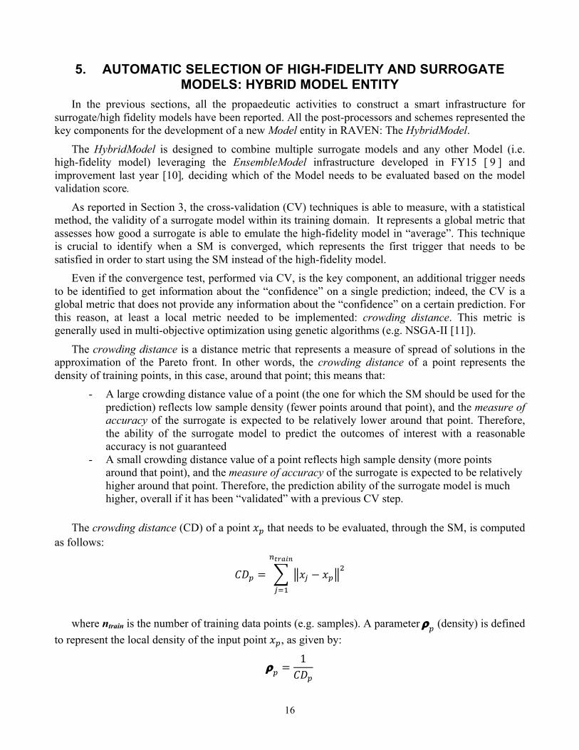
The crowding distance (CD) of a point 𝑥< that needs to be evaluated, through the SM, is computed

as follows:

𝐶𝐷< = 𝑥� − 𝑥<;

8��`��

�9:

where ntrain is the number of training data points (e.g. samples). A parameter r< (density) is defined

to represent the local density of the input point 𝑥<, as given by:

r< =1𝐶𝐷<

17

The parameter r<is then normalized to compute the distance coefficient 𝜶<, as given by:

𝛼< =max r − r<

min r −max r

The parameter 𝛼< (normalized between 0 and 1) represent the decision coefficient for determining if the SM evaluation can be accepted or rejected (𝛼< ≥ 𝛼��); practically, a threshold (𝛼��) of 0.2 is generally acceptable.

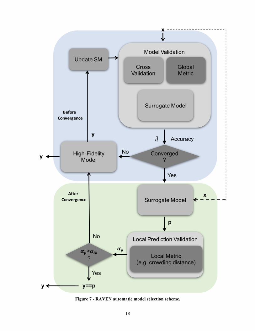
In summary, the HybridModel can be considered as a Petri-net [12] with N+1 nodes (1 high-fidelity model and N SMs) and a single gate (Validation Metrics).

Figure 7 shows the functional scheme of this new entity, for a single evaluation request 𝑥: 1) The SM is validated with a CV technique

2) If the SM is not converged (based on the calculated CV average distance 𝒅), the high-fidelity model gets inquired (y) and the new point is used to update the SM training set. The steps 1) and 2) are repeated for all the new evaluations until the CV convergence test is satisfied

3) SM is evaluated on the feature coordinates 𝒙, producing the outcome 𝒑; 4) The local prediction validation entity is inquired in order to estimate the validity of the

prediction 𝑎<;

5) If the prediction meets a user-define acceptability criterion, the outcome 𝒑 is kept and used as actual “true” value y;

6) If the prediction does not meet the user-defined acceptability criterion, the outcome 𝒑 is discarded and the high-fidelity model is inquired producing the “true” response 𝒚. The new “true” evaluation is added in the current SM training set and the SM is then reconstructed.

As inferable from the algorithm reported above, the HybridModel can speed up the Uncertainty Quantification and Probabilistic Risk Assessment without any loss of accuracy (within the user-defined accuracy levels).

18

Figure 7 - RAVEN automatic model selection scheme.

Model Validation

Cross Validation

Global Metric

Accuracy

Converged?

Update SM

High-Fidelity Model

Yes

No

x

!̅

Surrogate Model

y

Local Prediction Validation

Local Metric(e.g. crowding distance)

Surrogate Modelx

p

#$#$>#%&?

No

Yes

y==p

y

y

AfterConvergence

BeforeConvergence

19

6. APPLICATION EXAMPLES In order to test the correct implementation of all the schemes reported in previous chapters, several

different application analyses have been carried out. In order to define an analysis workflow, a single base accident scenario case has been considered for all the applications: a Station Black Out (SBO) accident of a Pressurized Water Reactor (PWR).

It is important to notice that the main goal of the results presented is to show the potential of the algorithms and schemes newly developed.

The following sections are organized as follows: - Section 6.2 describe the accident scenario that has been modeled/simulated and used as

base for all the following reported analyses - Section 6.2 shows the usage of the cross-validation post-processor for the assessment of the

global validity of the surrogate models - Section 6.3 shows the usage of the optimization scheme for SM parameters optimization

- Finally, Section 6.4 reports the application of the Hybrid Model for a Probabilistic Risk Assessment analysis for a PWR LOCA analysis

6.1 Description of the simulated scenario: SBO of a PWR In order to show the potential of the new capabilities, a SBO analysis for a prototypical PWR has

been considered. The accident scenario here considered is part of a larger analysis effort aimed to demonstrate a methodology for Multi-Unit PRA [13].

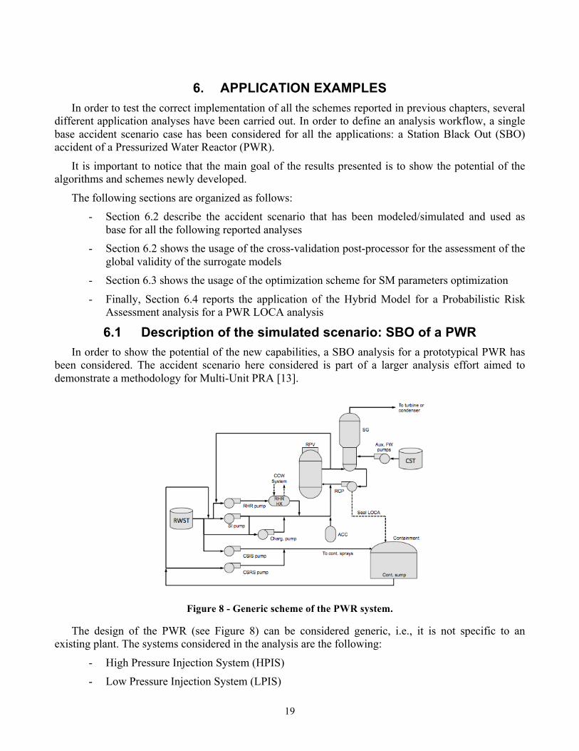
Figure 8 - Generic scheme of the PWR system.

The design of the PWR (see Figure 8) can be considered generic, i.e., it is not specific to an existing plant. The systems considered in the analysis are the following:

- High Pressure Injection System (HPIS) - Low Pressure Injection System (LPIS)

20

- Residual Heat Removal (RHR) system - Accumulators (ACCs)

- Auxiliary Feed-water (AFW) system - Charging pumps

In addition, two electrical switch-yards can provide electrical power to the unit. The unit has a set of Emergency Diesel Generators (EDGs) and, in addition, a swing EDG (i.e., EDGS) can be employed to provide an alternate AC power to the Unit.

More details about the systems can be found in Ref. [13]

6.1.1 Initiating Event The considered initiating event is a seismic event which causes the following events:

- Both switch-yards are disabled

- All EDGs are disabled except EDGS

- The seismic event might also rupture the SFPs. Thus a leak might bepresent during the accident scenario

Prior the seismic event, the PWR unit is at full power (100% power level). 6.1.2 Accident progression

Given the initiating event and the status of the plant, the analyzed accident focuses on the recovery strategy in order to place the PWR in a safe condition. For the scope of this scoping analysis, a unit is in safe state when EPEs are connected to the unit. These EPEs are located between the plant site boundaries and once connected to a unit can provide AC power and water injection.An EPE is available and it is assumed that the seismic event has not damaged it.

The PWR unit is in SBO condition but it has a good time margin before reaching Core Damage due to the fact that core injection can be employed for several hours.More details about the accident progression can be found in Ref. [13]. 6.1.3 PWR Model

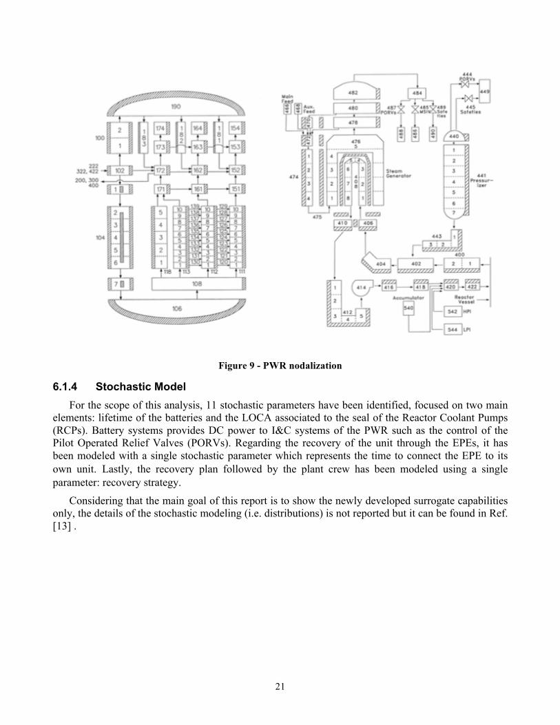
The accident sequence and, consequentially, the system has been modeled using RELAP5-3D [14]. The PWR model is based on the so-called INL Generic PWR (IGPWR) model [15]. The input deck is modeling a 2.5 GWth Westinghouse 460 3-loops PWR, including the RPV, the 3 loops and the primary and secondary sides of the steam generators (SGs) as shown in Figure 9. Four independent channels are used for representing the reactor core. Three channels model the active core and one channel models the core bypass. Different power values are assigned to the three core channels in order to take into account the radial power distribution. Passive and active heat structures simulate the heat transfer between the coolant and fuel, the structures and the secondary side of the IGPWR. The possible operator actions that can occur during a SBO event with the reactor at full power are implemented through the RELAP5-3D control logic. These actions include SG cool-down, feed and bleed, flow control, primary/secondary side emergency injection, etc.

21

Figure 9 - PWR nodalization

6.1.4 Stochastic Model For the scope of this analysis, 11 stochastic parameters have been identified, focused on two main

elements: lifetime of the batteries and the LOCA associated to the seal of the Reactor Coolant Pumps (RCPs). Battery systems provides DC power to I&C systems of the PWR such as the control of the Pilot Operated Relief Valves (PORVs). Regarding the recovery of the unit through the EPEs, it has been modeled with a single stochastic parameter which represents the time to connect the EPE to its own unit.Lastly, the recovery plan followed by the plant crew has been modeled using a single parameter: recovery strategy.

Considering that the main goal of this report is to show the newly developed surrogate capabilities only, the details of the stochastic modeling (i.e. distributions) is not reported but it can be found in Ref. [13] .

22

6.2 Cross Validation for trained Surrogate Model The application example here reported is aimed to show how a constructed surrogate model can be

used in conjunction with model validation techniques (see Section 3) in order estimate the model validity for Uncertainty Quantification and PRA analyses.

6.2.1 Cross-Validation for a constructed surrogate model

As previously mentioned, the infrastructure for surrogate model validation has been developed. In order to show how the newly implemented capability can be used to construct a usable surrogate model for uncertainty quantification and PRA, the accident scenario briefly described in the previous section has been simulated.

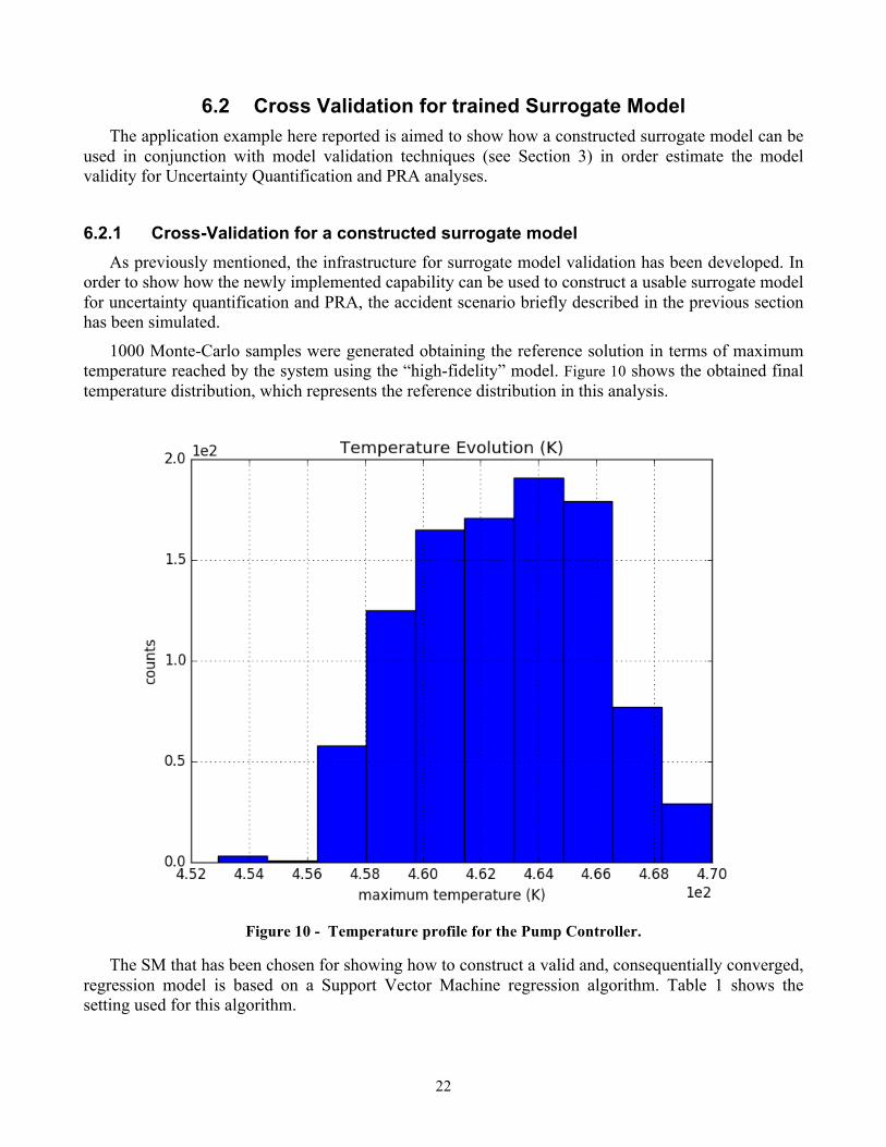
1000 Monte-Carlo samples were generated obtaining the reference solution in terms of maximum temperature reached by the system using the “high-fidelity” model. Figure 10 shows the obtained final temperature distribution, which represents the reference distribution in this analysis.

Figure 10 - Temperature profile for the Pump Controller.

The SM that has been chosen for showing how to construct a valid and, consequentially converged, regression model is based on a Support Vector Machine regression algorithm. Table 1 shows the setting used for this algorithm.

23

Table 1 - SVR SM settings.

Parameter Short description Value used

kernel Non-linear kernel Radial Basis Function

C Penalty parameter of the error term in the underneath optimization process 5.0

epsilon Epsilon-tube within which no penalty is associated in the training loss function with points predicted within a distance epsilon from the actual value.

0.1

gamma Kernel coefficient for the kernels “rbf” 0.1

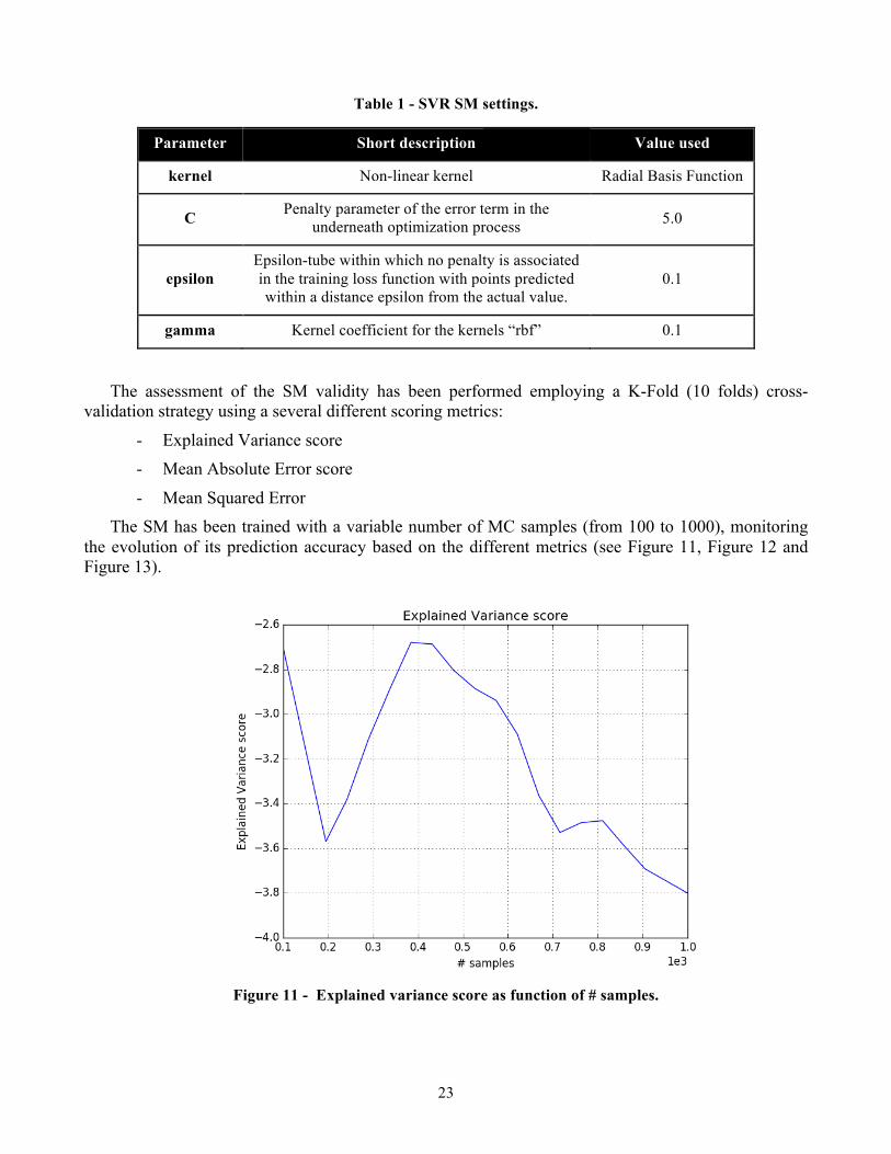
The assessment of the SM validity has been performed employing a K-Fold (10 folds) cross-validation strategy using a several different scoring metrics:

- Explained Variance score - Mean Absolute Error score

- Mean Squared Error The SM has been trained with a variable number of MC samples (from 100 to 1000), monitoring

the evolution of its prediction accuracy based on the different metrics (see Figure 11, Figure 12 and Figure 13).

Figure 11 - Explained variance score as function of # samples.

24

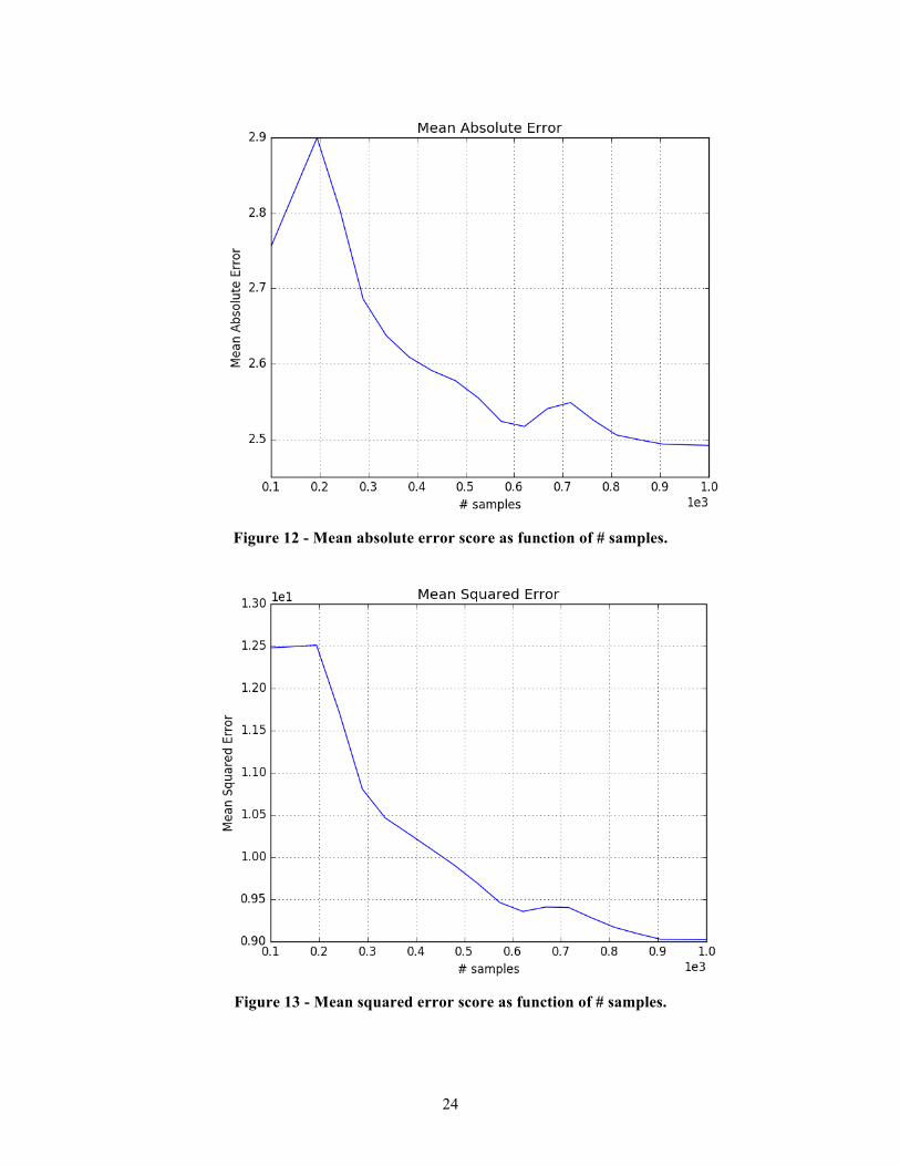
Figure 12 - Mean absolute error score as function of # samples.

Figure 13 - Mean squared error score as function of # samples.

25

Figure 11, Figure 12 and Figure 13 show the evolution of the score metrics as function of the number of training samples used for the surrogate construction. It can be seen that, after an initial oscillation of the metric scores (due to the too low number of samples), increasing the number of samples in the training set improves the prediction capabilities of the SM. Indeed, in Figure 11 it is shown how, with 1000 samples, the mean absolute error fells below 2.5 K.

6.3 Optimization of Surrogate Model Parameters In Section 4, it has been highlighted how the choice of a surrogate model (i.e. the particular

algorithm, the settings, etc.) can be challenging if the user is not completely familiar with the mathematical formulations of the surrogates of choice and the behavior, under combined uncertainties, of the system that he wants to surrogate (e.g. non-linear behavior, presence of discontinuities, etc.).

The optimization of the SM parameters is a key component to get a reliable regression model, overall when its usage is tight to PRA and UQ analyses.

In this section, an application example of the Optimization scheme for SM parameters is reported. The same SM (SVR) used in the previous section has been employed. The parameters that have been optimized are summarized in Table 2.

Table 2 - SVR SM parameters for the optimization.

Parameter Short description Value used

C Penalty parameter of the error term in the underneath optimization process 5.0

gamma Kernel coefficient for the kernels “rbf” 0.1

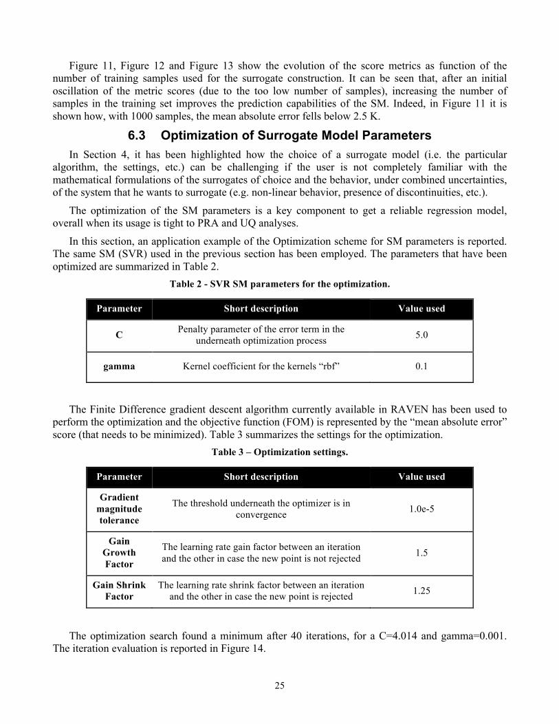
The Finite Difference gradient descent algorithm currently available in RAVEN has been used to perform the optimization and the objective function (FOM) is represented by the “mean absolute error” score (that needs to be minimized). Table 3 summarizes the settings for the optimization.

Table 3 – Optimization settings.

Parameter Short description Value used

Gradient magnitude tolerance

The threshold underneath the optimizer is in convergence 1.0e-5

Gain Growth Factor

The learning rate gain factor between an iteration and the other in case the new point is not rejected 1.5

Gain Shrink Factor

The learning rate shrink factor between an iteration and the other in case the new point is rejected 1.25

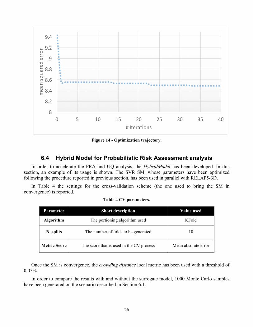
The optimization search found a minimum after 40 iterations, for a C=4.014 and gamma=0.001. The iteration evaluation is reported in Figure 14.

26

Figure 14 - Optimization trajectory.

6.4 Hybrid Model for Probabilistic Risk Assessment analysis In order to accelerate the PRA and UQ analysis, the HybridModel has been developed. In this

section, an example of its usage is shown. The SVR SM, whose parameters have been optimized following the procedure reported in previous section, has been used in parallel with RELAP5-3D.

In Table 4 the settings for the cross-validation scheme (the one used to bring the SM in convergence) is reported.

Table 4 CV parameters.

Parameter Short description Value used

Algorithm The portioning algorithm used KFold

N_splits The number of folds to be generated 10

Metric Score The score that is used in the CV process Mean absolute error

Once the SM is convergence, the crowding distance local metric has been used with a threshold of 0.05%.

In order to compare the results with and without the surrogate model, 1000 Monte Carlo samples have been generated on the scenario described in Section 6.1.

8

8.2

8.4

8.6

8.8

9

9.2

9.4

0 5 10 15 20 25 30 35 40

meansqua

rederror

#Iterations

27

When the HybridModel is used, of the 1000 Monte Carlo samples, only 200 were run using the RELAP5-3D model, resulting in a computational time reduction of 800*4 = 3200 CPU-hrs.

The comparison has been performed computing the main statistical moments. The results are summarized in Table 5 and Table 6.

Table 5 HybridModel statistical moments.

Parameter Result

mean 462.64

Minimum 458.57

Maximum 467.32

Median 462.64

Table 6 RELAP5-3D statistical moments

Parameter Result

mean 462.65

Minimum 458.03

Maximum 467.53

Median 462.64

The results show a very good agreement in terms of statistical moments and testify how promising this kind of techniques can be in order to tackle the computational burden of UQ and PRA with high-fidelity codes. The automatic model selection is illustrated in Figure 15.

28

Figure 15 - Automatic model selection for the first 200 runs (The value “1” indicates that we will execute

the surrogate while the value “0” indicates that we will execute RELAP5 model)

7. CONCLUSIONS The work that has been carried out in FY17 has been heavily focused on surrogate model

adaptivity. These activities are important to make the surrogate modeling techniques penetrate in the PRA and UQ world. The milestone of FY17 has been fully accomplished, delivering Global Validation methods, Local validation metrics, automatic optimization of surrogate parameters and, finally, an automatic scheme to switch between high-fidelity models and surrogates.

29

The RAVEN team is planning to extend the adaptive surrogate capabilities, introducing new metrics (local) that are close to the SM mathematical formulation instead of data points’ density.

8. REFERENCES

30

1. A Alfonsi, C Rabiti, D Mandelli, J Cogliati, RA Kinoshita, A Naviglio, “Dynamic event tree

analysis through Raven”, Idaho National Laboratory (INL) (2014) 2. A Alfonsi, C Rabiti, D Mandelli, J Cogliati, R Kinoshita, A Naviglio, “Hybrid Dynamic Event Tree

sampling strategy in RAVEN code”, Proceedings of International Topical Meeting on Probabilistic Safety Assessment (2015)

3. Joshua Joseph Cogliati, Jun Chen, Japan Ketan Patel, Diego Mandelli, Daniel Patrick Maljovec, Andrea Alfonsi, Paul William Talbot, Cristian Rabiti, “Time Dependent Data Mining in RAVEN”, INL/EXT-16-39860 (2016)

4. Scikit-learn: Machine Learning in Python, Pedregosa et al., JMLR 12, pp. 2825-2830, 2011.

5. Jie Zhang, Souma Chowdhury and Achille Messac, “An adaptive hybrid surrogate model”, Struct Multidisc Optim (2012) 46:223-238

6. A. Alfonsi, C. Rabiti, D. Mandelli, J. J. Cogliati, R. S. Sen, and C. L. Smith. Improving Limit Surface Search Algorithms in RAVEN Using Acceleration Schemes: Level II Milestone, Jul 2015.

7. A. J. Smola and B. Scholkopf, A tutorial on support vector regression, Statistics and Computing, vol. 14, no. 3, pp. 199–222, 2004.

8. Aaron S Epiney, Andrea Alfonsi, Cristian Rabiti, Jun Chen, “Economic Assessment of Nuclear Hybrid Energy Systems: Optimization using RAVEN”, 2017 Annual Meeting, American Nuclear Society (2017)

9. D. Mandelli, C. Smith, A. Alfonsi, C. Rabiti, J. Cogliati, H. Zhao, I. Rinaldi, D. Maljovec, P.Talbot, B. Wang, V. Pascucci. Reduced Order Model Implementation in the Risk-Informed Safety Margin CharacterizationToolkit. INL/EXT-15-36649

10. Andrea Alfonsi, Cristian Rabiti, Daniel Maljevoic, Diego Mandelli, Joshua Cogliati, “Enhancements to the RAVEN code in FY16”, INL/EXT-16-40094

11. K. Deb, A. Pratap, S. Agarwal, T. Meyarivan, “A fast and elitist multiobjective genetic algorithm: NSGA-II”, IEEE Transactions on Evolutionary Computation, Vol. 6 (2) (2002)

12. Petri, Carl Adam; Reisig, Wolfgang (2008). "Petri net". Scholarpedia. 3 (4): 6477. doi:10.4249/scholarpedia.6477

13. D. Mandelli, C. Parisi, A. Alfonsi, D. Maljovec, R. Boring, S. Ewing, S. St Germain, C. Smith, C. Rabiti, “Multi-Unit PRA: a Simulation-Based Approach”, submitted to Reliability Engineering & System Safety (2017)

14. C. B. Davis, "Assessment of RELAP5-3D Using Data from Two-Dimensional RPI Flow Tests," Proceedings from the 1998 RELAP5 International Users Seminar, College Station, Texas, May 17-21, 1998.

15. C. Parisi, S. R. Prescott, R. H. Szilard, J. L. Coleman, R. E. Spears, A. Gupta, “Demonstration of External Hazards Analysis”, Technical Report, Idaho National Laboratory Technical Report: INL/EXT-16-39353, 2016.