Demand Estimation and Household's Welfare...

r.t ~ *~ ~ * "f: *l iti liJf ~ ~ifB ~ *29%* 2 . 3 % 2006ip12Y=]

Demand Estimation and Household's Welfare Measurement :

Case Studies on Japan and Indonesia

Tri Widodo*

Abstract

This paper aims to estimate households' demand function and welfare

measurement under Linear Expenditure System (LES) in the case of Japan and

Indonesia. In estimating the coefficients of the LES, this paper applies Seeming

ly Uncorrelated Regression (SUR) method. This paper gives some conclusions.

First, for food consumption Indonesian households have the maximum mar

ginal budget share on Meat and the minimum one on Fruits; meanwhile

Japanese households have the maximum marginal budget share on Fish and

sellfish and the minimum one on Dairy products and eggs. Indonesian house

holds are 'meat lover' and Japanese households are 'fish lover'. Second, In

donesian households have smaller gap between minimum consumption (subsis

tence level) and average consumption than Japanese households have. Third,

with the same level of price increase on foods the simulation shows that in

nominal-term (Yen, ¥) Japanese households get greater welfare decrease than

Indonesian households get. However, in the percentage of total food expendi

ture, Indonesian households get greater welfare decrease than Japanese house

holds get. Fourth, for the period 2000-2004 the changes of prices in living

expenditure increased both Japanese All Households and Japanese Worker

Households more than ¥4, 500.

Keywords: Linear Expenditure System (LES), Seemingly Uncorrelated Regression (SUR),

Compensating Van'alion (CV), Equivalent Variation (EV).

* Doctoral Program, Graduate School of Economics, Hiroshima University of Economics, Hiroshima, Japan. The author would like to thank Prof. Masumi Hakogi, Prof. Toshiyuki Mizoguchi and all participants of discussion conducted at Hiroshima university of Economics June 27th, 2006 for helpful comments and corrections.

104

1. Introduction

An individual household gets welfare (utility) from its consumption of

goods and services, such as food, clothes, housing, fuel, light, water, furniture,

transportation and communication, education, recreation and so on. The idea

of standard of living relates to various elements of household's livelihood and

varies with income. When income was low as in Japan in the 1950s this could

be indicated mainly by the consumption level, especially of foods. After most

of the households were able to meet basic needs in the 1960s, household con

sumption on semi-durable and durable goods became measure of the standard

living (Mizoguchi, 1995). How many goods and services the individual house

hold might have access depends very much on many factors such as income,

prices of goods (complementary and substitution), availability of goods in

market, etc.

In the basic microeconomics theory, it is assumed that the individual

household wants to maximise its welfare (utility) subject to its income. It is

achieved by determining the optimal number of goods and services (Mas-Colell

et aI., 1995). Therefore, some changes not only in prices of goods and services

but also in the individual household's income will affect the individual house

hold's welfare. As the income increased as high as the other developed coun

tries in the 1970s, Japanese household's interest turned from current expendi

ture to financial and real assets for maintaining a stable life in the present and

in the future. Further, in such a higher income level country as Japan, house

holds start preferring leisure hours to overtime pay.

The prices of goods and services and income might be determined by

market mechanism or government intervention. By market mechanism means

that the prices of goods and services are determined by the interaction between

market supply and demand. In market, the prices will decrease if supply is

greater than demand (excess supply); in contrast, the prices will increase when

demand is greater than supply (excess demand). The government might control

the prices of goods and services for some reasons; such as equality in distribu

tion, pro-poor government policy, floor and ceiling prices policy (for example

in agricultural products: e.g.rice), efficiency, etc. The goods and services which

Demand Estimation and Household's Welfare Measurement: Case Studies on Japan and Indonesia 105

the prices are determined by the government are called administrated goods

(Tambunan, 2001). In Indonesia, for example, the government determines the

prices of fuel (Bahan Bakar Minyak, BBM), electricity, telephone, minimum

wage and so on. Therefore, estimation demand and welfare measurement of

the individual household are very interesting to be analysed.

This paper has some aims i.e. to derive a model of demand and welfare

measurement of an individual household; to estimate the model for Japan and

Indonesia cases; to make some simulation from the estimation. The rest of this

paper is organized as follows. Part 2 gives the theoretical framework that will

be used. Data and estimation method are presented in part 3. Research findings

will be presented in part 4. Finally, some conclusions are in part 5.

2. Theoretical Framework

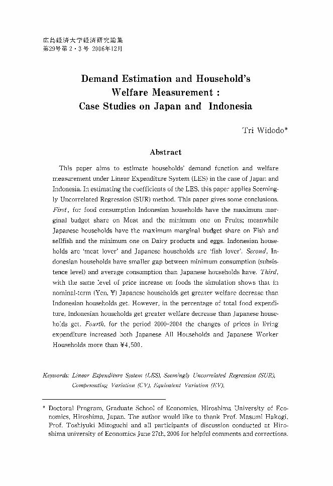
This paper will estimate the measurement of household welfare-change and

then use the estimation for analyzing the welfare impact of price changes due

to any shocks - such as government policies, economic crisis-in the case of

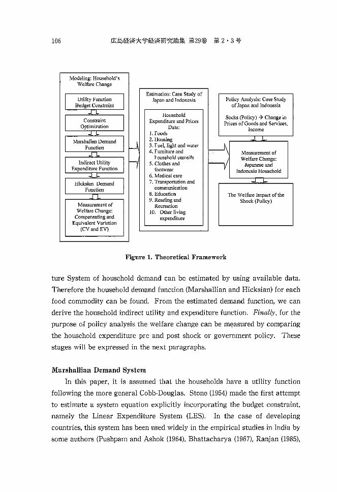
Japan and Indonesia. Figure 1 shows the theoretical framework of this paper.

The welfare analysis in this paper is mainly derived from the household

consumption. Theoretically, the household demand for goods and services is a

function of prices and income (by definition of Marshallian demand function).

Therefore, some changes in income and prices of goods and services will

directly affect the number of goods and services and indirectly affect household

welfare.

2.1. Estimating Demand, Indirect Utility and Expenditure Function

To get the measurement of welfare change, we have to estimate the

household expenditure function. For that purpose, some steps should be foll

owed. Firstly, the household utility function should be established. In this

paper, the household's utility function is assumed to be Cobb-Douglas function

which can derive the Linear Expenditure System of demand (LES) (Stone, 1954).

This assumption is taken because the Linear Expenditure System (LES) is (j)

suitable for the household consumption/demand. Secondly, the Linear Expendi-

106

Modeling: Household's Welfare Change

Estimation: Case Study of Utility Function Japan and Indonesia Policy Analysis: Case Study

Budget Constraint of Japan and Indonesia

L!. Household Constraint Expenditure and Prices

Socks (policy) ~ Change in Prices of Goods and Services,

Optimization Data: Income I. Foods

Marshalian Demand W 2. Housing

Function 3. Fuel, light and water -\ .LJ. 4. Furniture and Measurement of

household utensils

-vi Welfare Change:

Indirect Utility n 5. Clothes and Japanese and Expenditure Function footwear Indonesia Household

...!.....!- 6. Medical care

Hicksian Demand 7. Transportation and

Function communication

J J. 8. Education The Welfare Impact of the

Measurement of 9. Reading and Shock (Policy)

Recreation Welfare Change: 10. Other living

Compensating and expenditure Equivalent Variation

CCVandEV)

Figure 1. Theoretical Framework

ture System of household demand can be estimated by using available data.

Therefore the household demand function (Marshallian and Hicksian) for each

food commodity can be found. From the estimated demand function, we can

derive the household indirect utility and expenditure function. Finally, for the

purpose of policy analysis the welfare change can be measured by comparing

the household expenditure pre and post shock or government policy. These

stages will be expressed in the next paragraphs.

Marshallian Demand System

In this paper, it is assumed that the households have a utility function

following the more general Cobb-Douglas. Stone (1954) made the first attempt

to estimate a system equation explicitly incorporating the budget constraint,

namely the Linear Expenditure System (LES). In the case of developing

countries, this system has been used widely in the empirical studies in India by

some authors (Pushpam and Ashok (1964), Bhattacharya (1967), Ranjan (1985),


Satish and Sanjib (1999».

Formally the individual household's preferences defined on n goods are

characterized by a utility function of the Cobb-Douglas form. Klein and Rubin

(1948) formulated the LES as the most general linear formulation in prices and

income satisfying the budget constraint, homogeneity and Slutsky symmetry.

Basically, Samuelson (1948) and Geary (1950) derived the LES representing the

utility function:

U(Xl ...... xn)=(XI-X~)al(X2-x~y2(X3-X~)a3······(Xn-X~)an ........................... (1)

The individual household's problem is to choose Xi that can maximize its

utility U(Xl) subject to its budget constraint. Therefore, the optimal choice of

Xl is obtained as a solution to the constrained optimization problem as follows: n

Max U(X,)= II (Xl-X?)a,

Xl

Subject to:

PX::;:M

1=1

Solving the utility maximization problem, we can find the Marsha11ian

(uncompensated) demand function for each commodity Xl as follows:

al (M- ~PjxY) Xl=X?+ d- for all i and j .......................................... (2)

Pl~al 1=1

Where: i E (1,2, ...... n)

j E (1,2, ...... n) n

Since a restriction that the sum of parameters al equals to one, ~al=l, is 1=1

imposed equation (2) becomes:

al (M- ~PjxY) Xl=X?+ J- for all i and j .......................................... (3)

Pl

Equation (2) can be also reflected as the Linear Expenditure System as follows:

P1Xl =P1X? + al (M - ±PjxY) for all i and j ...................................... '(4) J=I

This equation system (4) can be interpreted as stating that expenditure on

good i , given as PIXI, can be broken down into two components. The first part

is the expenditure on a certain base amount x? of good i , which is the minimum

108

expenditure to which the consumer is committed (subsistence expenditure), PIX?

(Stone, 1954). Samuelson (1948) interpreted x? as a necessary set of goods

resulting in an informal convention of viewing xP as non-negative quantity.

The restriction of xP to be non-negative values however is unnecessarily

strict. The utility function is still defined whenever: Xl- x? > O. Thus the

interpretation of xP as a necessary level of consumption is misleading (Pollak,

1968). The x? allowed to be negative provides additional flexibility in allowing

price-elastic goods. The usefulness of this generality in price elasticity depends

on the level of aggregation at which the system is treated. The broader the

category of goods, the more probable it is that the category would be price

elastic. Solari (in Howe, 1954 : 13) interprets negativity of x? as superior or

deluxe commodities.

In order to preserve the committed quantity interpretation of the x?'s when n

some x? are negative, Solari (1971) redefines the quantity :l:PjX¥ as 'augmented j=1

supernumerary income' (in contrast to the usual interpretation as supernumer

ary income, regardless of the signs of the x?). Then, defining n* such that all

goods with is n * have positive x? and goods for i > n * are superior with negative n n

x?, Solari interprets :l:PjX¥ as supernumerary income and :l: pjXy as fictitious j=1 j=n+1

zncome. The sum of 'Solary-supernumerary income' and fictitious income

equals augmented supernumerary income. Although somewhat convoluted,

these redefinition allow the interpretation of 'Solari-supernumerary income' as

expenditure in excess of the necessary to cover committed quantities.

The second part is a fraction al of the supernumerary income, defined as the n

income above the 'subsistence income' :l:PjX¥ needed to purchase a base amount j=1

of all goods. The al are scaled to sum to one to simplify the demand functions.

The al is referred to as the marginal budget share, al/:l:al. It indicates the

proportion in which the incremental income is allocated.

Indirect Utility

The indirect utility function V(P,M) can be found by substituting the

Marshallian demand Xl (equation 3) into the utility function U(XI) (equation 1).


Therefore the indirect utility function is:

n al M- ~pjxY

(

( n ) )ai

V(P, M)= II j=1 for all i and j ···· .. ···· .. ······· .. ·········(5) I=a PI

Expenditure Function

Equation (5) shows the household's utility function as a function of income

and commodity prices. By inverting the indirect utility function the expendi

ture function E(P,U), which is a function of certain level of utility and commod

ity prices, can be expressed as follows:

E(P, U) n V + ±Plxf for all i and j ..................................... "(6) II (J!L) 1=1

1=1 PI

2.2. Welfare Change

Equivalent Variation (EV) and Compensating Variation (CV) will be

applied to analyze the impact of the price changes due to any shock or govern

ment policy. The Equivalent Variation (EV) can be defined as the dollar

amount that the household would be indifferent in accepting the changes in food

prices and income (wealth). It is the change in household's wealth that would

be equivalent to the prices and income change in term of its welfare impact (EV

is negative if the prices and income changes would make the household worse

off). Meanwhile, the Compensating Variation (CV) measures the net revenue of

the planner who must compensate the household for the food prices and income

changes, bringing the household back to its welfare (utility level) (Mas-Colell et

a1., 1995 : 82). The CV is negative if the planner would have to pay household

a positive level of compensation because the prices and income changes make

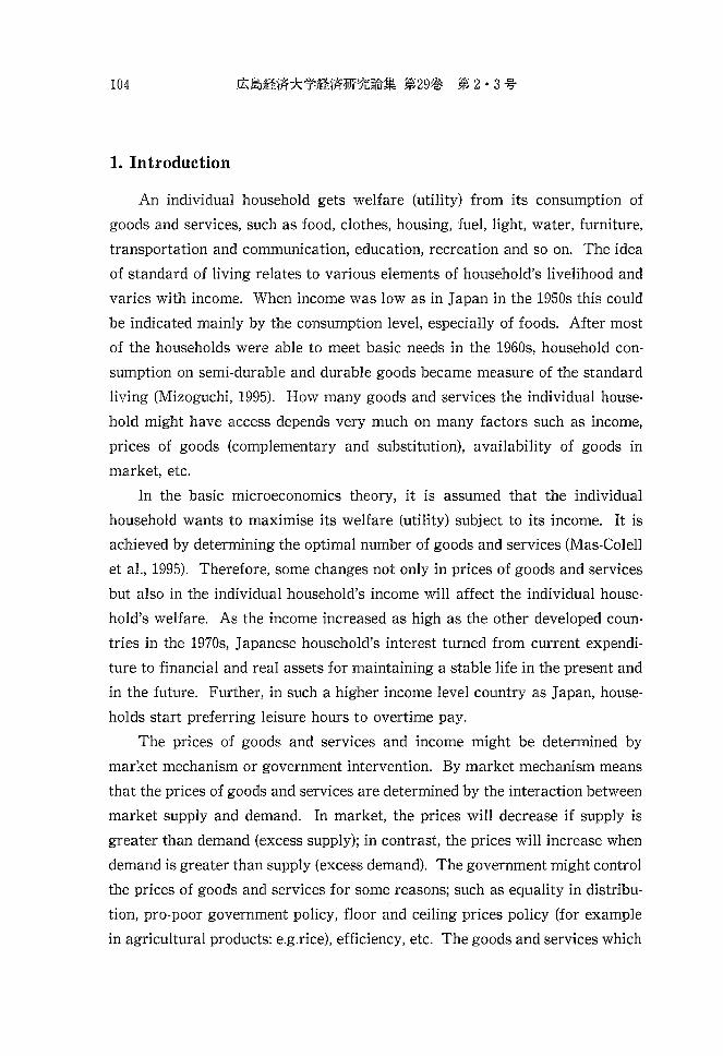
household worse off). Figure 2 visualizes the EV and CV when there is only an

increase in price of one good.

If there are changes in prices and income, the EV and CV can be formulated as: EV = F(pO, V') - E(p, U) + (M' - MO) ................................................ (7)

CV = E(pO, VO) - E(p', V) + (M' - MO) ................................................ (8)

In the context of Linear Expenditure System (LES), equation (7) and (8) become:

110

R

R

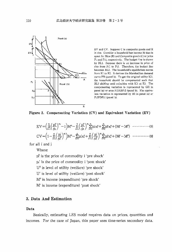
EV and CV. Suppose C is composite goods and R is rice. Consider a household has income M that is spent for Rice (R) and Composite goods (C) at price p, and P,l, respectively. The budget line is shown by ELL Suppose there is an increase in price of rice from Pel to P,2. Therefore, the budget line becomes EL2. The household's equilibrium moves from E1 to E2. It derives the Marshallian demand curve FE (panel b). To get the original utility IC1, the household should be compensated such that EL2 shifting until coincides with IC1 at E3. The compensating variation is represented by GH in panel (a) or area P,2AEPcl (panel b). The equivalent variation is represented by HI in panel (a) or P,2FDP,1 (panel b).

Figure 2. Compensating Variation (CV) and Equivalent Variation (EV)

EV=(IT (p?)a, -l)MO- IT (p?)a'i!Pix?+ i!p?x?+(M'- MO) ············ .. ·(9) 1=1 PI 1=1 PI i=1 1=1

CV=(l- IT (pi)a')MO- i!pix?+ IT (pi)ali!p?x?+(M'- MO) ···············(10) 1=1 PI 1=1 1=1 PI 1=1

for all i and j

Where:

pP is the price of commodity i 'pre shock'

PI' is the price of commodity i 'post shock'

VO is level of utility (welfare) 'pre shock'

V' is level of utility (welfare) 'post shock'

MO is income (expenditure) 'pre shock'

M' is income (expenditure) 'post shock'

3. Data And Estimation

Data

Basically, estimating LES model requires data on prices, quantities and

incomes. For the case of Japan, this paper uses time-series secondary data.


The data on yearly average monthly receipts and disbursement per household

(All household and Worker household) (in Yen) are taken from Annual Report

on the Family Income and Expenditure (Two or More Person Household) 1963

-2004 published by Statistics Bureau, Ministry of Internal Affairs and Commu

nication, japan.

The analysis is divided into two i.e. analysis on food expenditure and on

living expenditure. The food expenditure covers Cereal; Fish and shellfish;

Meat; Dairy products and eggs; Vegetable and seaweeds; Fruits; and Cooked

food. Meanwhile, the living expenditure covers: Food; Housing; Fuel, light and

water; Furniture and household utensils; Clothes and footwear; Medical care;

Transportation and communication; Education; Reading and recreation; and

Other living expenditure. The Other living expenditure consists of personal

care, toilet articles, personal effects, tobacco, etc.

Consumer Price Indexes (CPI) on food and living expenditure (subgroup

index) are taken from Annual Report on the Consumer Price Index 1963-2004

published by Statistics Bureau, Ministry of Internal Affairs and Communica

tion, japan. There are three year basis 1980=100; 1990=100 and 2000=100.

This paper converts the index into the same base year 2000=100 (base year

shifting). Prices of commodities on food and living expenditure are taken from

Annual Report on the Price Survey 2000 published by Statistics Bureau,

Ministry of Internal Affairs and Communication, japan. Food commodity

prices (Cereal; Fish and shellfish; Meat; Dairy products and eggs; Vegetable and

seaweeds; Fruits; and Cooked food) are then derived from the simple average

of two extreme prices of the items in 49 towns and villages in Japan. Prices of

living expenditure (Food, Housing, Fuel, light and water, Furniture and house

hold utensils, Clothes and footwear, Medical care, Transportation and commu

nication, Education, Reading and recreation, and Other living expenditure) are

derived from the weighted average of the items in 49 towns and villages in

Japan. This paper uses the weight from the Annual Report on the Consumer

Price Index 2000. Since the prices in 2000 derived, prices in the other years can

be calculated by using correspondence Consumer Price Index. Data on quantity

of goods or services consumed can be derived by dividing good or services

expenditure with related prices.

112

(2)

For the case study of Indonesia, this paper uses pooled (time series and

cross section, panel) secondary data about individual household's expenditure

from Rural Price Statistics (Statistik Harga Pedesaan) and Survey of Living Cost

(Survey Biaya Hidup) published by the Central Bureau of Statistics (Badan

Pusat Statistik, BPS) Indonesia 1980, 1981, 1984, 1987, 1990, 1993 and 1996. The

data used are consumption on foods, prices of foods, income (total expenditure)

of households. For the comparison proposes between Japan and Indonesia, this

paper uses the same kind of food products i.e. Cereal; Fish and shellfish; Meat;

Diary products and eggs; Vegetable and seaweeds; Fruits; and Cooked food.

There is no analysis of living expenditure due to the lack of availability of data

on prices of living expenditures in Indonesia.

Estimation

The estimation of a linear expenditure system (LES) shows certain compli

cations because, while it is linear in the variables, it is non-linear in the

parameters, involving the products of al and x? in equation systems (3) and (4).

There are several approaches to estimation of the system (Intriligator et aI.,

1996). The first approach determines the base quantities x? on the basis of

extraneous information or prior judgments. The system (4) then implies that

expenditure on each good in excess of base expenditure (PIXI-PIXP) is a linear

function of supernumerary income, so each of the marginal budget shares al can

be estimated applying the usual single-equation simple linear regression

methods.

The second approach reverses this procedure by determining the marginal

budget shares al on the basis of extraneous information or prior judgments (or

Engel curve studies, which estimate al from the relationship between expendi

ture and income). It then estimates the base quantities x? by estimating the

system in which the expenditure less the marginal budget shares time income

(PIXI- aiM) is a linear function of all prices. The total sum of squared errors -

over all goods as well all observations- is then minimized by choice of the x?

The third approach is an iterative one, by using an estimate of al condi

tional on the x? (as in the first approach) and the estimates of the xP conditional

on al (as in the second approach) iteratively so as to minimize the total sum of


squares. The process would continue, choosing al based on estimate xP and

choosing xP based on the last estimated ai, until convergence of the sum of

squares is achieved.

The fourth approach selects al and xP simultaneously by setting up a grid

of possible values for the 2n-1 parameters (the-1 based on the fact that the al n

sum tends to unity, ~al=l) and obtaining that point on the grid where the total 1=1

sum of squares over all goods and all observations is minimized.

This paper applies the fourth approach. The reason is that when estimat

ing a system of seemingly uncorrelated regression (SUR) equation, the estima

tion may be iterated. In this case, the initial estimation is done to estimate

variance. A new set of residuals is generated and used to estimate a new

variance-covariance matrix. The matrix is then used to compute a new set of

parameter estimator. The iteration proceeds until the parameters converge or

until the maximum number of iteration is reached. When the random errors

follow a multivariate normal distribution these estimators will be the maxi

mum likelihood estimators (Judge et aI., 1982: 324).

Rewriting equation (4) to accommodate a sample t= 1,2,3, ...... T and 10

goods yields the following econometric non-linear system:

PltXlt=PltX~t+ a1(M - ~pjx1)+elt J=l

P2tX2t=P2tX~t+ a2(M - ~pjx1) +e2t for all i and j .............................. (11) J=l

Where: elt is error term equation (good) i at time t.

Given that the covariance matrix EI et ef 1 ='; where e1 = (elt, elt, ...... e10t)

and'; is not diagonal matrix, this system can be viewed as a set of non-linear

seemingly unrelated regression (SUR) equations. There is an added complica-10

tion, however. Because ~Pltxlt=M the sum of the dependent variables is equal 1=1

to one of the explanatory variables for all t, it can be shown that (elt, e2t, ..... .

elOt)=O and hence'; is singular, leading to a breakdown in both estimation

114

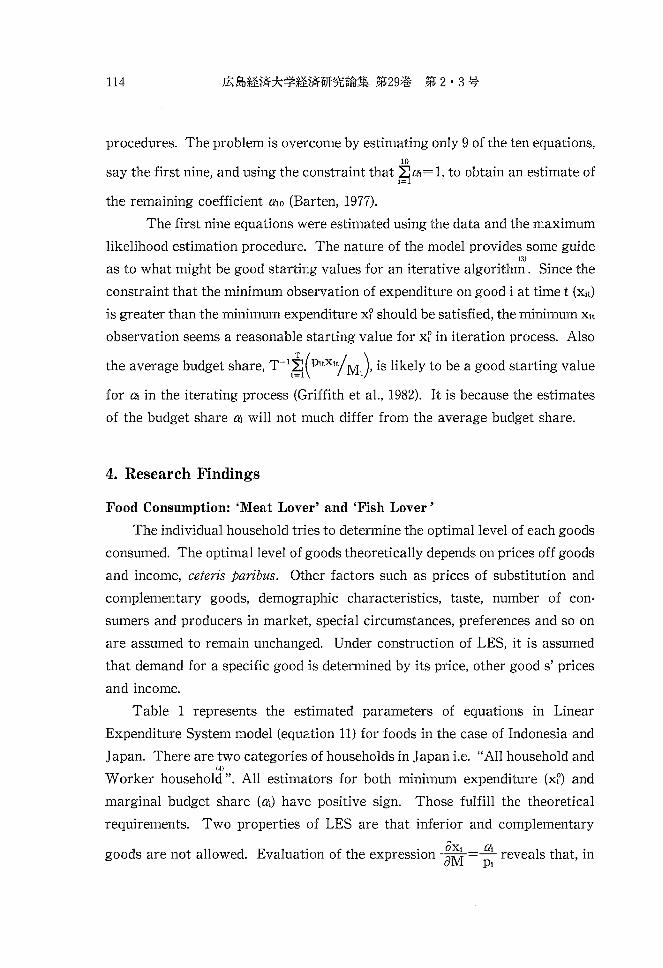
procedures. The problem is overcome by estimating only 9 of the ten equations, 10

say the first nine, and using the constraint that 2:al=l, to obtain an estimate of 1=1

the remaining coefficient alO (Barten, 1977).

The first nine equations were estimated using the data and the maximum

likelihood estimation procedure. The nature of the model provides some guide (3)

as to what might be good starting values for an iterative algorithm. Since the

constraint that the minimum observation of expenditure on good i at time t (Xlt)

is greater than the minimum expenditure x? should be satisfied, the minimum Xlt

observation seems a reasonable starting value for x? in iteration process. Also

the average budget share, T- 1i1(Pltxlt/MJ is likely to be a good starting value

for al in the iterating process (Griffith et aI., 1982). It is because the estimates

of the budget share al will not much differ from the average budget share.

4. Research Findings

Food Consumption: 'Meat Lover' and 'Fish Lover'

The individual household tries to determine the optimal level of each goods

consumed. The optimal level of goods theoretically depends on prices off goods

and income, ceteris paribus. Other factors such as prices of substitution and

complementary goods, demographic characteristics, taste, number of con

sumers and producers in market, special circumstances, preferences and so on

are assumed to remain unchanged. Under construction of LES, it is assumed

that demand for a specific good is determined by its price, other good s' prices

and income.

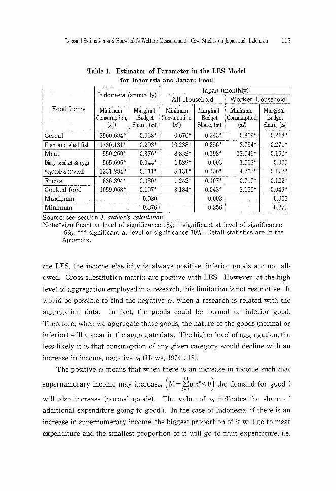
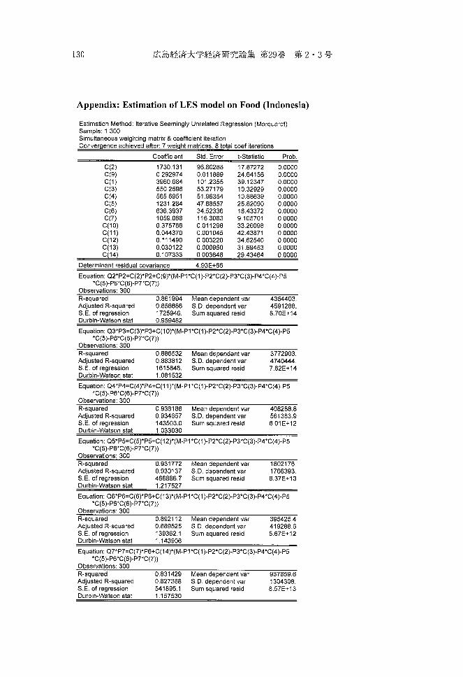
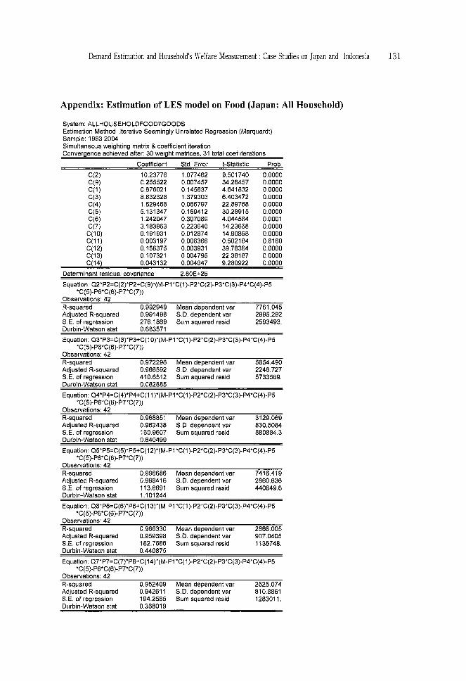
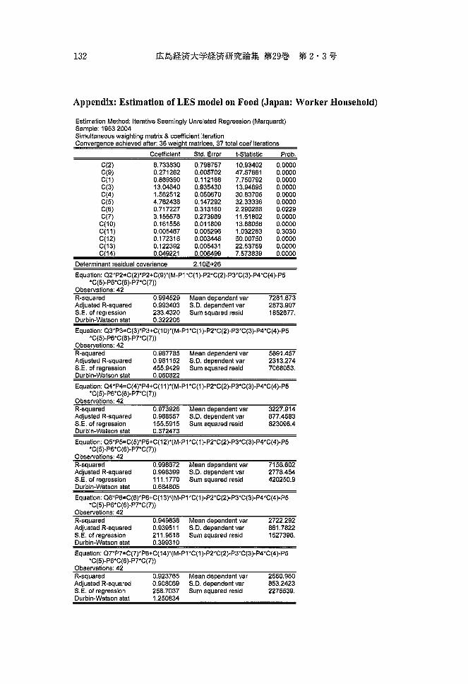
Table 1 represents the estimated parameters of equations in Linear

Expenditure System model (equation 11) for foods in the case of Indonesia and

Japan. There are two categories of households in Japan i.e. "All household and (4)

Worker household". All estimators for both minimum expenditure (x?) and

marginal budget share (al) have positive sign. Those fulfill the theoretical

requirements. Two properties of LES are that inferior and complementary

goods are not allowed. Evaluation of the expression g~ = ;: reveals that, in


Table 1. Estimator of Parameter in the LES Model for Indonesia and Japan: Food

Japan (monthly) Indonesia (annually)

All Household Worker Household

Food Items Minimmn Marginal Minimmn Marginal Minimum Marginal Consmnption, Budget Consmnption, Budget Consmnption, Budget

(x?) Share, (£1'1) (x?) Share, (ai) (x?) Share, (£1'1)

Cereal 3960.684* 0.038* 0.676* 0.243* 0.869* 0.218*

Fish and shellfish 1730.131* 0.293* 10.238* 0.256* 8.734* 0.271 *

Meat 550.260* 0.376* 8.832* 0.192* 13.046* 0.162*

Diary product & eggs 565.695* 0.044* 1.529* 0.003 1.563* 0.005

Vegetable & seaweeds 1231.284* 0.111 * 5.131 * 0.156* 4.762* 0.172*

Fruits 636.394* 0.030* 1.242* 0.107* 0.717* 0.122*

Cooked food 1059.068* 0.107* 3.184 * 0.043* 3.156* 0.049*

Maximum 0.030 0.003 0.005

Minimum 0.376 0.256 0.271

Source: see section 3, author's calculation Note:*significant at level of significance 1%; **significant at level of significance

5%; *** significant at level of significance 10%. Detail statistics are in the Appendix.

the LES, the income elasticity is always positive, inferior goods are not all

owed. Cross substitution matrix are positive with LES. However, at the high

level of aggregation employed in a research, this limitation is not restrictive. It

would be possible to find the negative ai, when a research is related with the

aggregation data. In fact, the goods could be normal or inferior good.

Therefore, when we aggregate those goods, the nature of the goods (normal or

inferior) will appear in the aggregate data. The higher level of aggregation, the

less likely it is that consumption of any given category would decline with an

increase in income, negative aj (Howe, 1974 : 18).

The positive aj means that when there is an increase in income such that

supernumerary income may increase, (M - j~PjX~ < 0) the demand for good i

will also increase (normal goods). The value of aj indicates the share of

additional expenditure going to good i. In the case of Indonesia, if there is an

increase in supernumerary income, the biggest proportion of it will go to meat

expenditure and the smallest proportion of it will go to fruit expenditure, i.e.

116

37.6 percent and 3 percent, respectively. Indonesian households can be referred

as 'meat lover' households. In contrast, Japanese households (both All house

holds and Worker households), the highest marginal budget share is for Fish

and shellfish and the minimum one is for Dairy product and eggs i.e. 27.1

percent and 0.5 percent. Japanese households can be identified as 'fish lover'

households. If there is increase in supernumerary income, 27.1 percent of it will

be allocated for fish and sellfish expenditure.

The minimum consumption (xf) of both Indonesian and Japanese cases are

not comparable because the data (quantity and value) used are different from

each other i.e. currency, prices and unit of measurements. To make it compa

rable, this paper constructs the ratio between minimum consumption (x?) and o

average consumption (AC), in notation: CR = tC' The minimum consumption (5)

(xf) can be defined as the amount of goods consumed by the 'poorest household',

meanwhile the average consumption (AC) can be interpreted as the amount of

goods consumed by the 'average household'.

The ratio can be seen as an indicator of 'gap' between the minimum and the

average expenditures (or 'gap' between the 'poorest household' and the 'average

household' consumption). The ratio will lie between zero and one. The ratio

CR will be close to one when the minimum consumption x? is close to the

average. There is no much difference between the minimum consumption and

the average consumption. In contrast, the ratio CR will close to zero when the

minimum consumption x? is far from to the average. It is theoretically hoped,

the households in developed countries which have a high level on non-food

consumption, will have relatively lower CR ratio than the households in devel

oping countries which still have problems in food fulfillment. Households in

developed countries have a larger variety of food consumption than household

in developing countries. Japanese consumers are increasingly looking for

diversity and high quality food choices (Agriculture and Agri-Food Canada,

2005).

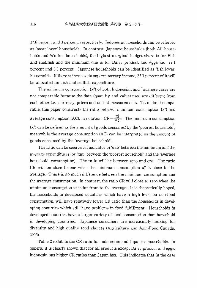
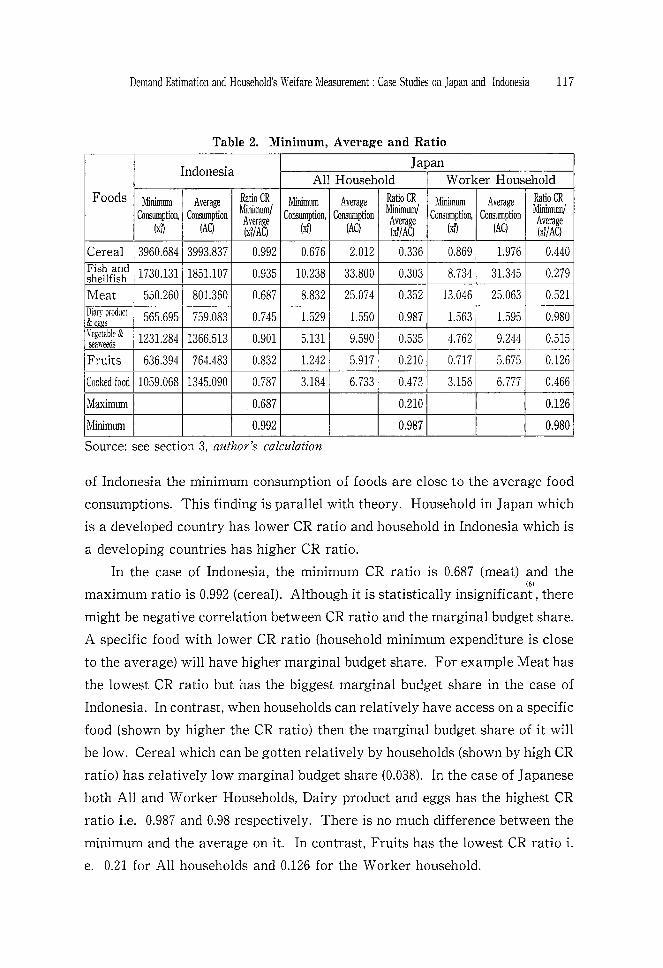
Table 2 exhibits the CR ratio for Indonesian and Japanese households. In

general it is clearly shown that for all products except Dairy product and eggs,

Indonesia has higher CR ratios than Japan has. This indicates that in the case


Table 2. Minimum, Average and Ratio

Indonesia Japan

All Household Worker Household Foods Minimum Average Ratio CR Minimum Average Ratio CR Minimum Average Ratio CR

Consumption, Consumption Minimum/ Consumption, Consumption Minimum/ Consumption, Consumption Minimum! Average Average Average

(x1) (AC) (x1/AC) (xn (AC) (xf/AC) (x1) (AC) (x1/AC)

Cereal 3960.684 3993.837 0.992 0.676 2.012 0.336 0.869 1.976 0.440 Fish and 1730.131 1851.107 0.935 10.238 33.800 0.303 8.734 31.345 0.279 shellfish

Meat 550.260 801.360 0.687 8.832 25.074 0.352 13.046 25.063 0.521 Diary product 565.695 759.083 0.745 1.529 1.550 0.987 1.563 1.595 0.980 & eggs \'egetable & 1231.284 1366.513 0.901 5.131 9.590 0.535 4.762 9.244 0.515 seaweeds

Fruits 636.394 764.483 0.832 1.242 5.917 0.210 0.717 5.675 0.126

Cooked food 1059.068 1345.090 0.787 3.184 6.733 0.473 3.156 6.777 0.466

Maximum 0.687 0.210 0.126

Minimum 0.992 0.987 0.980

Source: see section 3, author's calculation

of Indonesia the minimum consumption of foods are close to the average food

consumptions. This finding is parallel with theory. Household in Japan which

is a developed country has lower CR ratio and household in Indonesia which is

a developing countries has higher CR ratio.

In the case of Indonesia, the minimum CR ratio is 0.687 (meat) and the 161

maximum ratio is 0.992 (cereal). Although it is statistically insignificant, there

might be negative correlation between CR ratio and the marginal budget share.

A specific food with lower CR ratio (household minimum expenditure is close

to the average) will have higher marginal budget share. For example Meat has

the lowest CR ratio but has the biggest marginal budget share in the case of

Indonesia. In contrast, when households can relatively have access on a specific

food (shown by higher the CR ratio) then the marginal budget share of it will

be low. Cereal which can be gotten relatively by households (shown by high CR

ratio) has relatively low marginal budget share (0.038). In the case of Japanese

both All and Worker Households, Dairy product and eggs has the highest CR

ratio i.e. 0.987 and 0.98 respectively. There is no much difference between the

minimum and the average on it. In contrast, Fruits has the lowest CR ratio i.

e. 0.21 for All households and 0.126 for the Worker household.

118

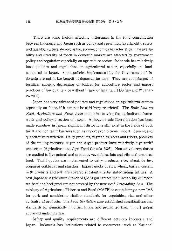
There are some factors affecting differences in the food consumption

between Indonesia and Japan such as policy and regulation (availability, safety

and quality), culture, demographic, socio-economic characteristics. The availa

bility and diversity of foods in domestic market are affected by government

policy and regulation especially on agriculture sector. Indonesia has relatively

loose policies and regulations on agricultural sector, especially on food,

compared to Japan. Some policies implemented by the Government of In

donesia are not in the benefit of domestic farmers. They are abolishment of

fertilizer subsidy, decreasing of budget for agriculture sector and import

practices of low quality rice without illegal or legal tariff (Arfian and Wijanar

ko 2000).

Japan has very advanced policies and regulations on agricultural sectors

especially on foods, if it can not be said 'very restricted'. The Basic Law on

Food, Agriculture and Rural Area maintains to give the agricultural frame

work and policy direction of Japan. Although trade liberalization has been

made somehow in Japan, significant distortions still exist in the fields of both

tariff and non tariff barriers such as import prohibitions, import licensing and

quantitative restriction. Dairy products, vegetables, roots and tubers, products

of the milling industry, sugar and sugar product have relatively high tariff

protection (Agriculture and Agri-Food Canada 2005). Non ad-valorem duties

are applied to live animal and products, vegetables, fats and oils, and prepared

food. Tariff quotas are implemented to dairy products, rice, wheat, barley,

prepared edible fat and starches. Import guota of rice, wheat, barley, certain

milk products and silk are covered substantially by state-trading entities. A

new Japanese Agriculture Standard (JAS) guarantees the traceability of impor

ted beef and beef products not covered by the new Beef Traceability Law. The

ministry of Agriculture, Fisheries and Food (MAFF) is establishing a new JAS

for pork and considering similar standards for vegetables, rice and other

agricultural products. The Food Sanitation Law established specifications and

standards for genetically modified foods, and prohibited their import unless

approved under the law.

Safety and quality requirements are different between Indonesia and

Japan. Indonesia has institutions related to consumers -such as National


Consumer Protection Institution (Badan Perlindungan Konsumen Nasional

BPKN), Indonesian Consumer Institution Foundation (Yayasan Lembaga Kon

sumen Indonesia YLKI), National Consumer Protection Institution Foundation

(Yayasan Lembaga Perlindungan Konsumen Nasional YLPKN), Indonesian

cosumer Advocating Institution (Lembaga Advokasi Konsumen Indonesia

(LAKI) etc- but they are relatively powerless in intervening policy or regulation

related to consumers. Law No. 8/1999 about Consumer Protection was estab

lished. Nevertheless, the implementation is still far from perfect. A Consumer

co-cooperative is a valuable lesson from Japanese case. The Japanese move

ment of cooperatives goes back to the 19th century when the first consumer

cooperative was established in 1896. Today, the Japanese consumer co

operatives have established themselves as a major force in the retailing indus

try, foods are the dominant products for them. The Japanese Consumers'

Co-operative Union (JCCU) develops its own food standards, much stricter than

those imposed by the government and ensures that food and co-op brand

products supplied by their members meet its own standards for safety and

quality (JCCU 2002-2003). The revision of the Food Sanitation Law and the

passage of the new Basic Law for Food Safety in 2003 gave consumer co

operatives a central role in food safety (JCCU, 2002-2003). In the past (New

Order regime), Indonesia had many kinds of co-operatives including consumer

co-cooperative. But they did not develop well because the governments used

them as 'political commodity'.

Religions, geography, climate and cultural belief, basic nutritional require

ments and the unaccountable elements of tastes and preferences might affect

the development of a particular country's eating habits and cuisine. In the

Japanese case, it might be guessed that fish and seafood - both fresh and

preserved- play an important dietary role in daily life. Generally speaking,

Japanese are supposed to enjoy meals with their eyes. 'Nature' and 'harmony'

are words used to represent Japanese food which is served in a very artistic and

three-dimensional way. With preference put on freshness and natural flavour,

Japanese people love foods and ingredients that are at their 'shun' (now-in

season). They believe that eating the ingredients that are at their 'shun' will be

good for the health and spiritual life.

120

The japanese food culture is also influenced by religious beliefs. Despite

much longer existence of Shinto and Confucianism, Buddhism became the

official religion of japan in the sixth century. During the following 1,200 years,

meat was a prohibited food to the japanese because Buddhist teaching did not

allow killing of animals for food. Meat was allowed for sale and consumption

only after the Meiji Restoration in 1867. Although meat is widely consumed,

only certain cuts are preferred (Agriculture and Agri-Food Canada 2005). In

contrast, Moslem religion is the dominant religion in Indonesia. Indonesia is

the biggest Moslem country in the world. At least, there are two big religion

days of Islam i.e. Idul Fitri and Idul Adha. In the Idul Adha, Moslem people

cut sheep and cow for sacrificing and distribute them to the society. Idul Fitri

is the holy day celebrating the end of the fasting time holly Ramadan. In the

Idul Fitri, Indonesian moslem households always serve delicious foods in which

the ingredient is meat.

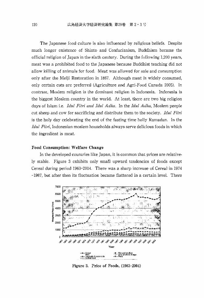
Food Consumption: Welfare Change

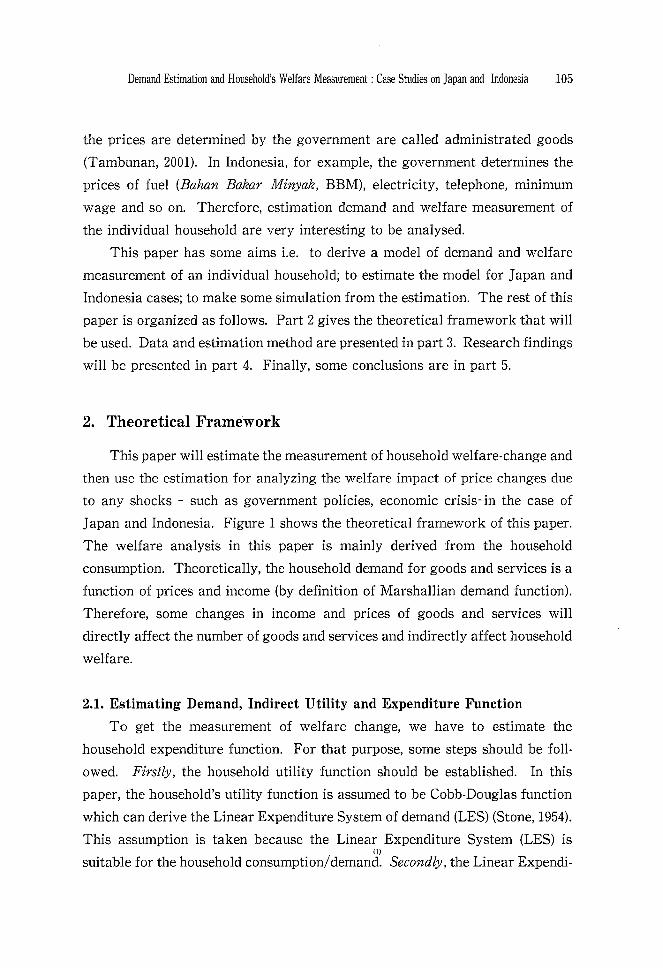
In the developed countries like japan, it is common that prices are relative

ly stable. Figure 3 exhibits only small upward tendencies of foods except

Cereal during period 1963-2004. There was a sharp increase of Cereal in 1974

-1987, but after then its fluctuation became flattered in a certain level. There

6000 +--"--~-,---:--:-------- ..... ---~--'--l

_ 5000 c

~ ~ 4000rr--'-c Il.

~ 3000 .!!'

~ 2000 +----c--=-=*'~,------------___ -_,_l

~~#~~##~~#~#~~$~~~~##

-- -~Cereal Meat

-.- Vegetable & seaweeds -+--- Cooked food

Year

_____ Fish and shellfish ~ ~Z products & eggs

Figure 3. Price of Foods, (1963-2004)


has been change in food consumption (Agriculture and Agri-Food Canada 2005).

Due to rapid economic growth in the 1960s and 1970s, the traditional way of

eating, reliant on rice and fish, gradually shifted towards new food products

such as livestock and dairy products. The mid-1980s saw the emergence of a

variety of processed foods and the proliferation of fast food restaurants. In

1990s, there were change in dining pattern from the traditional form of dining

at home at a fixed time with all household members present to 'flexible meal

pattern' with family members having own meals at different times to suit their

lifestyles and schedules. These development leads to a strong preference for

processed foods and eating out.

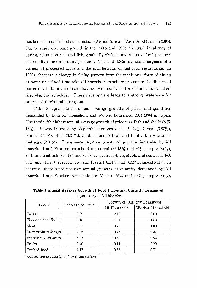
Table 3 represents the annual average growths of prices and quantities

demanded by both All household and Worker household 1963-2004 in Japan.

The food with highest annual average growth of price was Fish and shellfish (5.

16%). It was followed by Vegetable and seaweeds (5.07%), Cereal (3.87%),

Fruits (3.40%), Meat (3.21%), Cooked food (2.17%) and finally Diary product

and eggs (2.05%). There were negative growth of quantity demanded by All

household and Worker household for cereal (-2.13% and -2%, respectively),

Fish and shellfish (-1.51% and -1.53, respectively), vegetable and seaweeds (-0.

89% and -1.92%, respectively) and Fruits (-0.14% and -0.39% respectively). In

contrast, there were positive annual growths of quantity demanded by All

household and Worker Household for Meat (0.75% and 0.47% respectively),

Table 3 Annual Average Growth of Food Prices and Quantity Demanded (in percent/year), 1963-2004

Foods increase of Price Growth of Quantity Demanded


Cereal 3.89 -2.13 -2.00

Fish and shellfish 5.16 -1.51 -1.53

Meat 3.21 0.75 1.00

Dairy products & eggs 2.05 0.47 0.47

Vegetable & seaweeds 5.07 -0.89 -0.92

Fruits 3.40 -0.14 -0.39

Cooked food 2.17 0.66 0.71

Source: see section 3, author's calculation

122

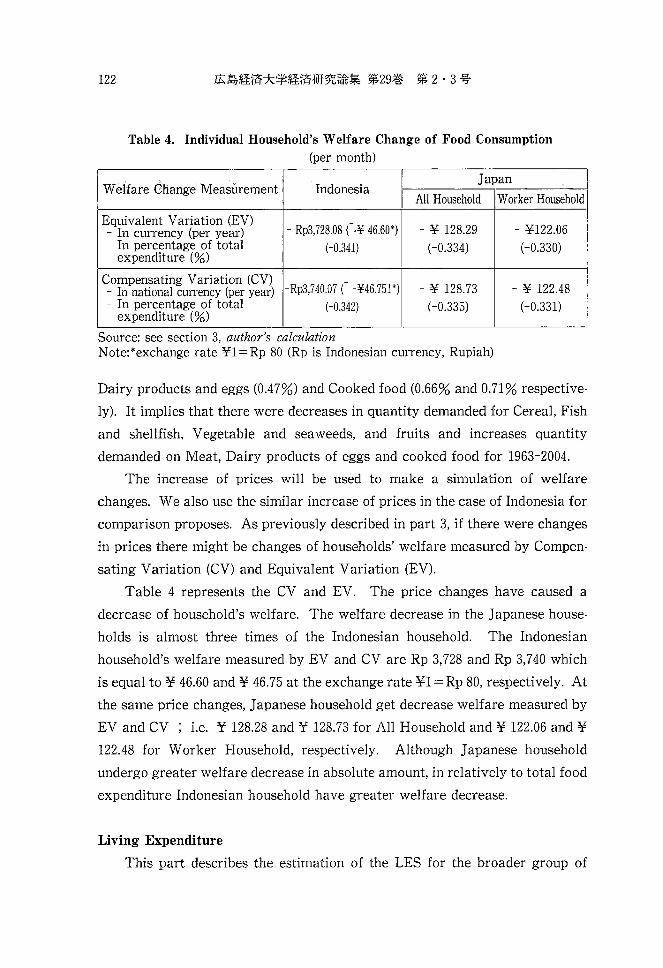
Table 4. Individual Household's Welfare Change of Food Consumption (per month)

WeIfare Change Measurement Indonesia Japan


Equivalent Variation (EV) - Rp3,728.08 c·¥ 46.60*) - ¥ 128.29 - ¥122.06 - In currency (per year)

- In percentage of total (-0.341) (-0.334) (-0.330) expenditure (%)

Compensating Variation (CV) -Rp3,740.07 C -¥46.751*) - ¥ 128.73 - ¥ 122.48 - In national currency (per year)

- In percentage of total (-0.342) (-0.335) (-0.331) expenditure (%)

Source: see section 3, author's calculation Note:*exchange rate ¥l=Rp 80 (Rp is Indonesian currency, Rupiah)

Dairy products and eggs (0.47%) and Cooked food (0.66% and 0.71% respective

ly). It implies that there were decreases in quantity demanded for Cereal, Fish

and shellfish, Vegetable and seaweeds, and fruits and increases quantity

demanded on Meat, Dairy products of eggs and cooked food for 1963-2004.

The increase of prices will be used to make a simulation of welfare

changes. We also use the similar increase of prices in the case of Indonesia for

comparison proposes. As previously described in part 3, if there were changes

in prices there might be changes of households' welfare measured by Compen

sating Variation (CV) and Equivalent Variation (EV).

Table 4 represents the CV and EV. The price changes have caused a

decrease of household's welfare. The welfare decrease in the Japanese house·

holds is almost three times of the Indonesian household. The Indonesian

household's welfare measured by EV and CV are Rp 3,728 and Rp 3,740 which

is equal to ¥ 46.60 and ¥ 46.75 at the exchange rate ¥1 = Rp 80, respectively. At

the same price changes, Japanese household get decrease welfare measured by

EV and CV ; i.e. ¥ 128.28 and ¥ 128.73 for All Household and ¥ 122.06 and ¥

122.48 for Worker Household, respectively. Although Japanese household

undergo greater welfare decrease in absolute amount, in relatively to total food

expenditure Indonesian household have greater welfare decrease.

Living Expenditure

This part describes the estimation of the LES for the broader group of


expenditure than food expenditure previously analyzed i.e. living expenditure

in the case of Japan. We do not analyze Indonesian case because there is no

data on prices of living expenditure. The living expenditure consists of Food;

Housing; Fuel, light and water charges; Furniture and household utensils;

Clothes and Footwear; Medical care; Transportation and communication;

Education; Reading and recreation; and Other living expenditure. The Other

living expenditure consists of personal care services, toilet articles, personal

effects, tobacco, etc.

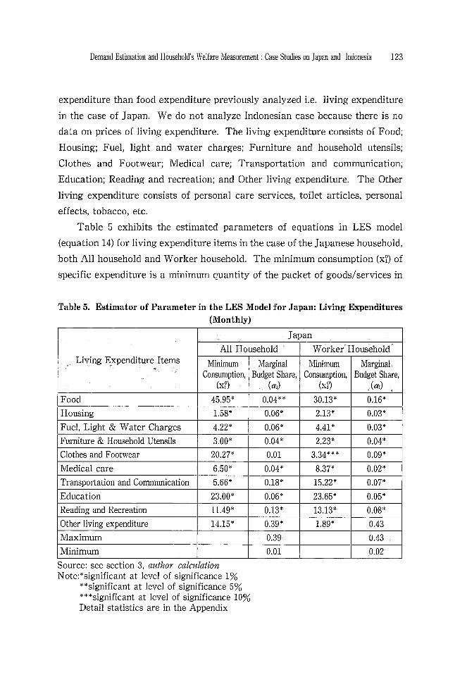
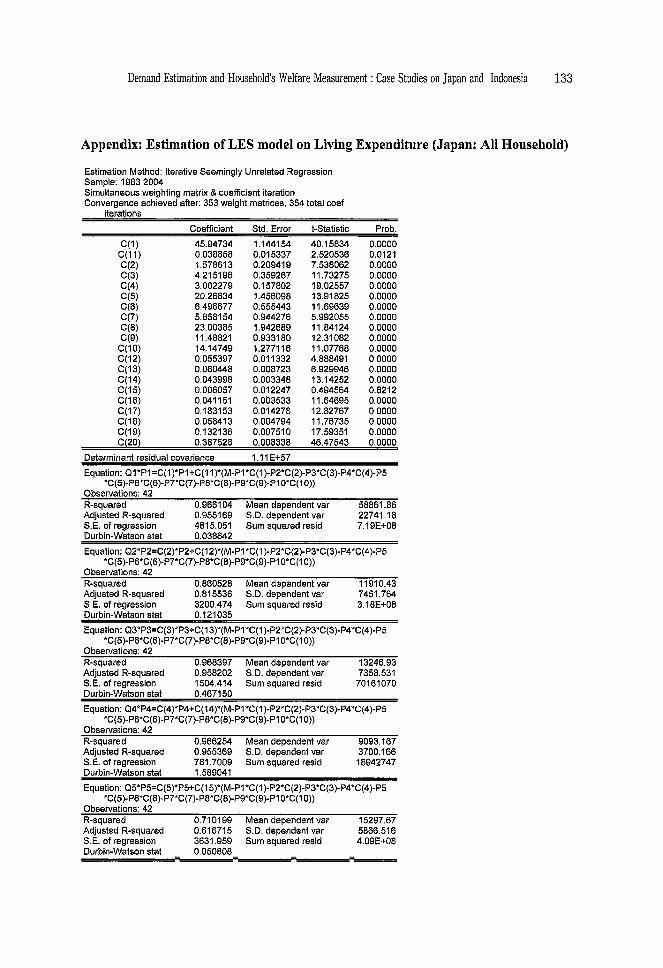
Table 5 exhibits the estimated parameters of equations in LES model

(equation 14) for living expenditure items in the case of the Japanese household,

both All household and Worker household. The minimum consumption (x~) of

specific expenditure is a minimum quantity of the packet of goods/services in

Table 5. Estimator of Parameter in the LES Model for Japan: Living Expenditures (Monthly)

Japan

All Household Worker Household Living Expenditure Items Minimum

Consumption, (x?)

Food 45.95*

Housing 1.58*

Fuel, Light & Water Charges 4.22*

Furniture & Household Utensils 3.00*

Clothes and Footwear 20.27*

Medical care 6.50*

Transportation and Communication 5.66*

Education 23.00*

Reading and Recreation 11.49*

Other living expenditure 14.15*

Maximum

Minimum

Source: see section 3, author calculation N ote:*significant at level of significance 1%

**significant at level of significance 5% ***significant at level of significance 10% Detail statistics are in the Appendix

Marginal Minimum Marginal Budget Share, Consumption, Budget Share,

(al) (xf) (al)

0.04** 30.13* 0.16*

0.06* 2.13* 0.03*

0.06* 4.41 * 0.03*

0.04* 2.23* 0.04*

0.01 3.34*** 0.09*

0.04* 8.37* 0.02*

0.18* 15.22* 0.07*

0.06* 23.65* 0.05*

0.13* 13.13* 0.08*

0.39* 1.89* 0.43

0.39 0.43

0.01 0.02

124

the specific category consumed by individual household in a month. Therefore,

if we want to know the minimum expenditure we just need to multiply the (7)

minimum consunption with corres ponding general price.

All estimators both minimum consumptions (x?) and marginal budget share

(£<'1) have positive sign. Those fulfill the theoretical requirements. All

estimators are significant less than 1% level of significance except minimum

consumption of Clothes and footwear in the case of Worker household which is

significant at 10% level of significance. In addition, the marginal budget share

of Clothes and footwear in the case of All household and the marginal budget

share of Other living expenditure are statistically insignificant. The last two

rows of Table 5 represents maximum and minimum values of marginal budget

share of the All household and the Worker household. The maximum marginal

budget share is for other living expenditure, i.e 0.39 for the All household and

0.43 for the Worker household. It means that if there is an additional supernu

merary income, the expenditure on Miscellaneous will get highest proportion.

1200

1)00

.00

600

400

200

~Focd

-Housing

Fuel. Ugh! & WaleI Charges

-~ Furniture & Household Utensils

--r- Clothes and Footwear

-Medical care

-+- Transportation and Corrm.mication

-Education

~ Reading and Recreation

ooL-______________________________________ +-__ -J Miscellaneous/Other living expenditure

~#~~~#~~~~~##~~#~#~~~ Year

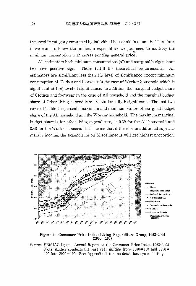
Figure 4. Consumer Price Index: Living Expenditure Group, 1963-2004 (2000=100)

Source: SBMIAC· Japan, Annual Report on the Consumer Price Index 1963-2004. Note: Author conducts the base year shifting from 1980=100 and 1990= 100 into 2000= 100. See: Appendix 1 for the detail base year shifting


Welfare Change Simulation: Japan 2000-2004

Figure 4 exhibits Consumer Price Index (CPI) for Living Expenditure

Group: Food; Housing; Fuel, light and water charges; Furniture and household

utensils; Clothes and footwear; Medical care; Transportation and communica

tion; Education; Reading and recreation; and Miscellaneous. It is interesting to

analyse the change in CPI for living expenditure group especially 'before' and

'after' 2000. Furniture and household utensil had the highest index before 2000

and it becomes the lowest after 2000. The index of Furniture and household has

downward tendency since 1993. In contrast, Education had lowest index before

2000 and it becomes the highest after 2000. The index of Eduction has an

upward tendency.

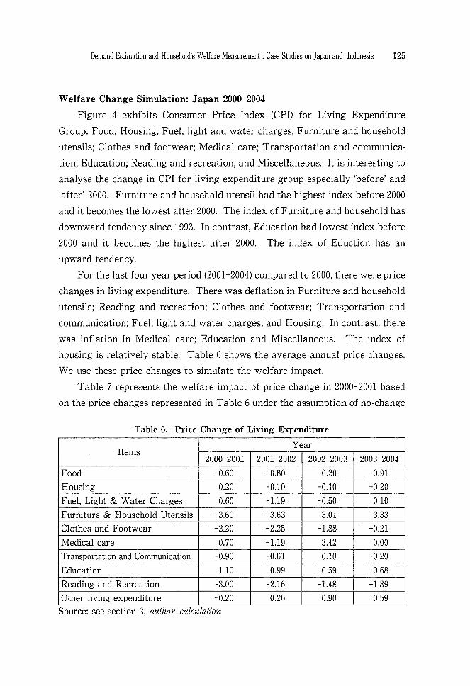
For the last four year period (2001-2004) compared to 2000, there were price

changes in living expenditure. There was deflation in Furniture and household

utensils; Reading and recreation; Clothes and footwear; Transportation and

communication; Fuel, light and water charges; and Housing. In contrast, there

was inflation in Medical care; Education and Miscellaneous. The index of

housing is relatively stable. Table 6 shows the average annual price changes.

We use these price changes to simulate the welfare impact.

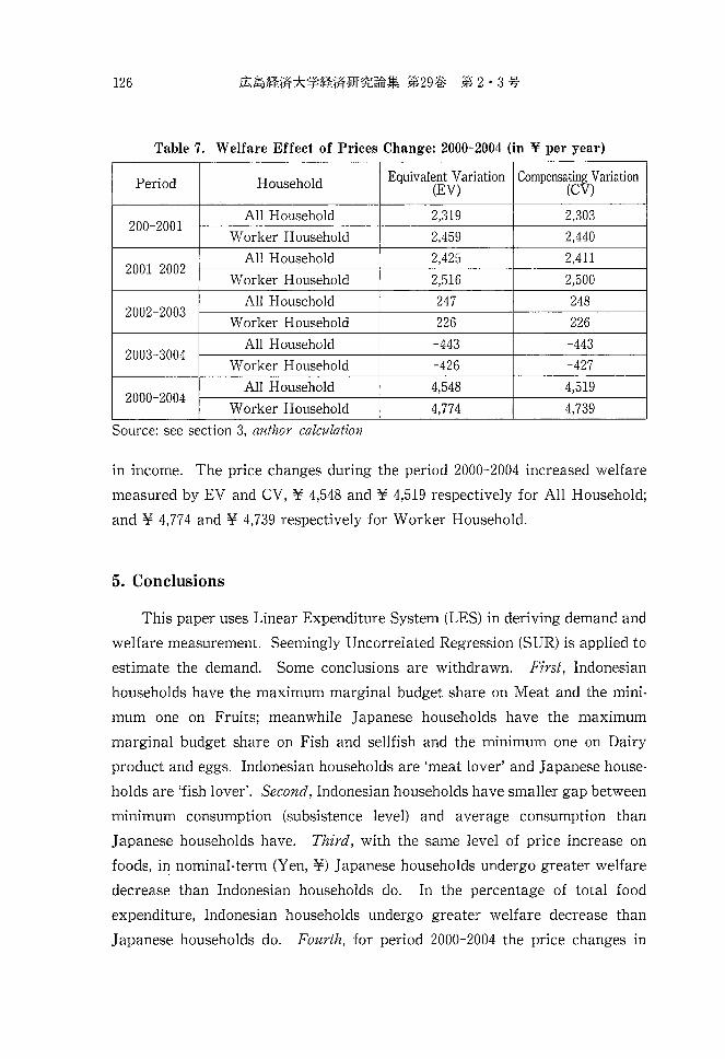
Table 7 represents the welfare impact of price change in 2000-2001 based

on the price changes represented in Table 6 under the assumption of no-change

Table 6. Price Change of Living Expenditure

Year Items

2000-2001 2001-2002 2002-2003 2003-2004

Food -0.60 -0.80 -0.20 0.91

Housing 0.20 -0.10 -0.10 -0.20

Fuel, Light & Water Charges 0.60 -1.19 -0.50 0.10

Furniture & Household Utensils -3.60 -3.63 -3.01 -3.33

Clothes and Footwear -2.20 -2.25 -1.88 -0.21

Medical care 0.70 -1.19 3.42 0.00

Transportation and Communication -0.90 -0.61 0.10 -0.20

Education 1.10 0.99 0.59 0.68

Reading and Recreation -3.00 -2.16 -1.48 -1.39

Other living expenditure -0.20 0.20 0.90 0.59

Source: see section 3, author calculatzon

126

Table 7. Welfare Effect of Prices Change: 2000-2004 (in ¥ per year)

Period Household Equivalent Variation Compensating Variation (EV) (CV)

All Household 2,319 2,303 200-2001

Worker Household 2,459 2,440

All Household 2,425 2,411 2001-2002


All Household 247 248 2002-2003

Worker Household 226 226

All Household -443 -443 2003-3004

Worker Household -426 -427

All Household 4,548 4,519 2000-2004


Source: see section 3, author calculation

in income. The price changes during the period 2000-2004 increased welfare

measured by EV and CV, ¥ 4,548 and ¥ 4,519 respectively for All Household;

and ¥ 4,774 and ¥ 4,739 respectively for W or ker Household.

5. Conclusions

This paper uses Linear Expenditure System (LES) in deriving demand and

welfare measurement. Seemingly Uncorrelated Regression (SUR) is applied to

estimate the demand. Some conclusions are withdrawn. First, Indonesian

households have the maximum marginal budget share on Meat and the mini

mum one on Fruits; meanwhile Japanese households have the maximum

marginal budget share on Fish and sellfish and the minimum one on Dairy

product and eggs. Indonesian households are 'meat lover' and Japanese house

holds are 'fish lover'. Second, Indonesian households have smaller gap between

minimum consumption (subsistence level) and average consumption than

Japanese households have. Third, with the same level of price increase on

foods, in nominal-term (Yen, ¥) Japanese households undergo greater welfare

decrease than Indonesian households do. In the percentage of total food

expenditure, Indonesian households undergo greater welfare decrease than

Japanese households do. Fourth, for period 2000-2004 the price changes in


living expenditure increased welfare for both All Household and Worker

Household.

For future study, a research might consider number of family member

(household size) for example one-person and two or more person household. In

the literature, it is called demographic equivalent scale. This can show us the

marginal living cost of the one additional household's member. Another

research can be also conducted for several different groups of household for

example: income group, location (district, rural-urban), etc.

Notes

(1) For detailed information, see Barten (1977), Deaton and Muellbauer (1980), Philips (1993)

and Deaton (1986).

(2) This paper does not take into account the variation of areas (urban and rural) and times.

It is simply assumed that there are no differences within areas and time. See Gudjarati

(2000) for detail explanation about panel-data models.

(3) For a detailed explanation about iterative algorithms, see Griffith et al 1982.

(4) Mizoguchi (1995) states that the 1959 National Survey of Family Income and Expenditure

(Zenkoku Shohi Jittai Chosa), NISFIE, was the first effort to capture household expenditure

in rural area because the Family Income and Expenditure Survey (Kakei Chosa), FIES, was

restricted to the urban area before 1962. As in the FIES, forestry, farming and fishery

households were not included in the NSFIE sample frame but were included after the 1984

survey. Therefore, the recent NISFE covers nearly all households in Japan in the popula

tion frame.

(5) By construction of LES, a poorest household is the household which consume in the

minimum amolmt of goods (subsistence level, x?).

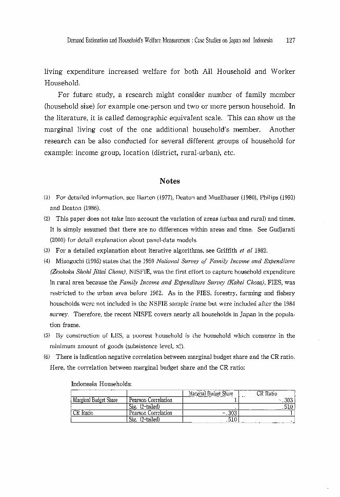
(6) There is indication negative correlation between marginal budget share and the CR ratio.

Here, the correlation between marginal budget share and the CR ratio:

Indonesia Households:

Marginal Budget Share CR Ratio Marginal Budget Share Pearson Correlation 1 -.303

Sig. (2-tailed) .510 CR Ratio Pearson Correlation -.303 1

Sig. (2-tailed) .510

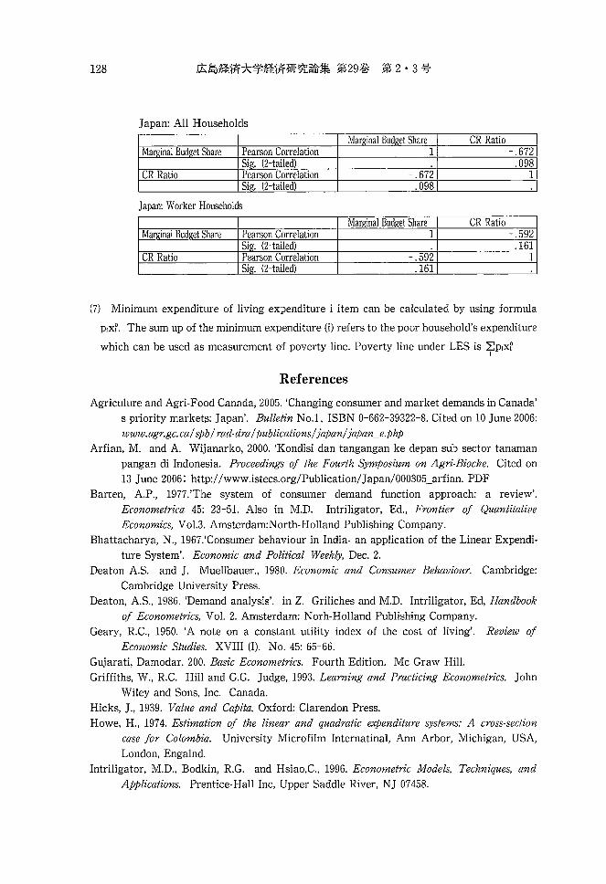
128

Japan: All Households


Sig. (Hailed) .098 CR Ratio Pearson Correlation -.672 1

Sig. (Hailed) .098

Japan: Worker Households


Sig. (Hailed) .161 CR Ratio Pearson Correlation -.592 1

Sig. (Hailed) .161

(7) Minimum expenditure of living expenditure i item can be calculated by using formula

PIX? The sum up of the minimum expenditure (i) refers to the poor household's expenditure

which can be used as measurement of poverty line. Poverty line under LES is ::EPIX? I

References

Agriculure and Agri-Food Canada, 2005. 'Changing consumer and market demands in Canada' s priority markets: Japan'. Bulletin No.1, ISBN 0-662-39322-8. Cited on 10 June 2006:

www.agr.gc.ca/spb/ rad-dra/ publications/ japan/japan_e.php Arfian, M. and A. Wijanarko, 2000. 'Kondisi dan tangangan ke depan sub sector tanaman

pangan di Indonesia. Proceedings of the Fourth Symposium on Agri-Bioche. Cited on

13 June 2006: http://www.istecs.org/PublicationlJ apan/000305_arfian. PDF Barten, A.P., 1977.'The system of consumer demand function approach: a review'.

Econometrica 45: 23-51. Also in M.D. Intriligator, Ed., Frontier of Quantitative Economics, Vo1.3. Amsterdam:North-Holland Publishing Company.

Bhattacharya, N., 1967.'Consumer behaviour in India- an application of the Linear Expendi

ture System'. Economic and Political Weekly, Dec. 2. Deaton A.S. and]. Muellbauer., 1980. Economic and Consumer Behaviour. Cambridge:

Cambridge University Press. Deaton, A.S., 1986. 'Demand analysis'. in Z. Griliches and M.D. Intriligator, Ed, Handbook

of Econometrics, Vol. 2. Amsterdam: Norh-Holland Publishing Company. Geary, R.C., 1950. 'A note on a constant utility index of the cost of living'. Review of

Economic Studies. XVIII (1). No. 45: 65-66. Gujarati, Damodar. 200. Basic Econometrics. Fourth Edition. Mc Graw Hill.

Griffiths, W., R.C. Hill and G.G. Judge, 1993. Learning and Practicing Econometrics. John Wiley and Sons, Inc. Canada.

Hicks, ]., 1939. Value and Capita, Oxford: Clarendon Press. Howe, H., 1974. Estimation of the linear and quadratic expenditure systems: A cross-section

case for Colombia. University Microfilm Internatinal, Ann Arbor, Michigan, USA,

London, Engalnd. Intriligator, M.D., Bodkin, R.G. and Hsiao,C., 1996. Econometric Models, Techniques, and

Applications. Prentice-Hall Inc, Upper Saddle River, NJ 07458.


JCCU (Japanese Consumers' Cooperative Union). 2002-03. Co-op for a Better Tomorrow. JCCU (Japanese Consumers' Cooperative Union). 2002-03. Co-op Fact and Figure. Judge, G.G., Hill. RC., Griffiths. W.E. Helmut,L., and Lee.T.e., 1982. Introduction to the

Theory and Practice of Econometrics. John Wiley and Sons, Inc. Canada Klein, L.R, and Rubin, H., 1948. 'A constant utility index of the cost of living'. Review of

Economic Studies. XV (2). No. 38: 84-87.

Mas-Colell, A, Whinston, M.D. and Green, lR, 1995. Microeconomic Theory. Oxford University Press. New York.

Mizoguchi, T., 1995. Reform of Statistical System under Socio-Economic Changes: Overview of Statistical Data in Japan. Maruzen Co., Ltd. Tokyo, Japan.

Philips, L., 1993. Applied Consumption Analysis. Revised and enlarged ed. Amsterdam: North Holland Publishing Company.

Pollak, RA, 1968. 'Additive utility function and linear Engel curves'. Discussion Paper. No 53, Department of Economics, University of Pennsylvania, revised Feb.

Puspham, P. and Ashok, R, 1964. "Demand elasticity for food grain'. Economic and Political Weekly. Nov. 28.

Ranjan, R. 1985. 'A dynamic analysis of expenditure pattern in mral India'. Journal of Development Economics. Vol. 19.

Samuelson, P.A ,1948. 'Some implication of linearity'. Review of Economic Studies. XV (2).

No. 38: 88-90

Samuelson, P.A dan Nordhaus, W.D., 2001. Microeconomics. Seventeenth Edition. McGrawHill. New York:.

Satish, Rand Sanjib, P., 1999. 'An analysis of consumption expenditure of rural and urban income groups in LES framework. ASIAN Economies.

Solari, L., 1971. ThOrie des Choir; et Fonctions de Consommation Semi-Agregees: Modeles Statiques. Geneve: Librairie Droz: 59-63.

Stone, R., 1954. 'Linear expenditure system and demand analysis: an application to the pattern of Britissh demand.' Economic Journal. 64: 511-27.

Tamblman, Tulus, 2000. Perekonomian Indonesia. Ghalia Indonesia. Jakarta. The Central Bureau of Statistics (Badan Pusat Statistik, BPS) of Indonesia, 1980, 1981, 1984,

1987, 1990, 1993, 1996. Statistik Harga Konsumen Pedesaan Di Java Dan Sepuluh Provinsi Luar Java (Rural Consumer Price Statistics in Java and Ten Provinces Out of Java). Jakarta.

__ , 1980, 1981, 1984, 1987, 1990, 1993, 1996. Survey Biaya Hidup (Survey of Living Cost). Jakarta.

130

Appendix: Estimation of LES model on Food (Indonesia)

Estimation Method: Iterative Seemingly Unrelated Regression (Marquardt) Sample: 1 300 Simultaneous weighting matrix & coefficient iteration Convergence achieved after: 7 weight matrices, 8 total coef iterations

Coefficient Std. Error t-Statistic Prob.

C(2) C(9) C(1) C(3) C(4) C(5) C(6) C(7)

C(10) C(11) C(12) C(13) C(14)

1730.131 0.292974 3960.684 550.2596 565.6951 1231.284 636.3937 1059.068 0.375768 0.044370 0.111490 0.030122 0.107333

Determinant residual covariance

96.80288 0.011889 101.2355 53.27179 51.96354 47.68557 34.52336 116.3083 0.011298 0.001045 0.003220 0.000950 0.003646

4.93E+66

17.87272 24.64156 39.12347 10.32929 10.88639 25.82090 18.43372 9.105701 33.26098 42.43871 34.62540 31.69453 29.43464

0.0000 0.0000 0.0000 0.0000 0.0000 0.0000 0.0000 0.0000 00000 0.0000 0.0000 0.0000 0.0000

Equation: Q2*P2=C(2)*P2+C(9)*(M-P1*C( 1 )-P2*C(2)-P3*C(3)-P4 *C( 4 )-P5 *C(5)-P6*C(6)-P7*C(7»

Observations: 300 R-squared 0.861994 Adjusted R-squared 0.858686 S. E. of regression 1725946. Durbin-Watson stat 0.959482

Mean dependent var S.D. dependentvar Sum squared resid

4354403. 4591288. 8.70E+14

Equation: Q3*P3=C(3)*P3+C(1 0)*(M-P1 *C(1 )-P2*C(2)-P3*C(3)-P4*C(4 )-P5 *C(5)-P6*C(6)-P7*C(7»

Observations: 300 R-squared Adjusted R-squared S. E. of regression Durbin-Watson stat

0.886532 0.883812 1615846. 1.081532


3772903. 4740444. 7.62E+14

Equation: Q4*P4=C(4)*P4+C(11 )*(M-P1*C(1 )-P2*C(2)-P3*C(3)-P4*C(4)-P5 *C(5)-P6*C(6)-P7*C(7»

Observations: 300 R-squared Adjusted R-squared S.E. of regression Durbin-Watson stat

0.936186 0.934657 143503.0 1.033030


408288.8 561383.9 6.01 E+12

Equation: Q5*P5=C(5)*P5+C(12)*(M-P1 *C(1 )-P2*C(2)-P3*C(3)-P4*C(4 )-P5 *C(5)-P6*C(6)-P7*C(7»


0.931772 0.930137 466886.7 1.217527


1802176. 1766393. 6.37E+13

Equation: Q6*P6=C(6)*P6+C(13)*(M-P1 *C( 1 )-P2*C(2)-P3*C(3)-P4 *C(4 )-P5 *C(5)-P6*C(6)-P7*C(7»


0.892112 0.889525 139362.1 1.143906


395425.4 419288.6 5.67E+12

Equation: Q7*P7=C(7)*P6+C( 14 )*(M-P1*C( 1 )-P2*C(2)-P3*C(3)-P4 *C(4 )-P5 *C(5)-P6*C(6)-P7*C(7»


0.831429 0.827388 541895.1 1.157530


937859.6 1304308. 8.57E+13

Demand Estimation and Household's Welfare Measurement: Case Studies on Japan and Indonesia l31

Appendix: Estimation ofLES model on Food (Japan: All Household)

System: ALLHOUSEHOLDFOOD7GOODS Estimation Method: Iterative Seemingly Unrelated Regression (Marquardt) Sample: 1963 2004 Simultaneous weighting matrix & coefficient iteration Convergence achieved after: 30 weight matrices, 31 total coef iterations


C(2) 10.23776 1.077462 9.501740 0.0000 C(9) 0.255522 0.007457 34.26457 0.0000 C(1) 0.676021 0.145637 4.641832 0.0000 C(3) 8.832328 1.379303 6.403472 0.0000 C(4) 1.529488 0.066797 22.89768 0.0000 C(5) 5.131347 0.169412 30.28915 0.0000 C(6) 1.242047 0.307089 4.044584 0.0001 C(7) 3.183863 0.223640 14.23658 0.0000 C(10) 0.191931 0.012874 14.90898 0.0000 C(11) 0.003197 0.006366 0.502184 0.6160 C(12) 0.156375 0.003931 39.78364 0.0000 C(13) 0.107321 0.004795 22.38187 0.0000 C(14) 0.043132 0.004647 9.280922 0.0000

Determinant residual covariance 2.80E+26

Equation: Q2*P2=C(2)*P2+C(9)*(M-P1*C(1 )-P2*C(2)-P3*C(3)-P4 *C(4 )-P5 'C(5)-P6*C(6)-P7*C(7»


0.992949 0.991498 276.1869 0.683571


7761.045 2995.292 2593493.

Equation: Q3*P3=C(3)*P3+C(1 0)*(M-P1*C(1 )-P2*C(2)-P3*C(3)-P4*C(4 )-P5 *C(5)-P6*C(6)-P7*C(7»


0.972296 0.966592 410.6512 0.082885


5854.490 2246.727 5733569.

Equation: Q4*P4=C(4 )*P4+C(11 )*(M-P1*C(1 )-P2*C(2)-P3*C(3)-P4*C(4 )-P5 *C(5)-P6'C(6)-P7*C(7»


0.968851 0.962438 160.9607 0.640499


3129.069 830.5084 880884.3

Equation: Q5*P5=C(5)*P5+C(12)*(M-P1*C(1 )-P2*C(2)-P3*C(3)-P4 *C(4 )-P5 'C(5)-P6*C(6)-P7*C(7»

Observations: 42 R-squared 0.998686 Adjusted R-squared 0.998416 S.E. of regression 113.8691 Durbin-Watson stat 1.101244


7416.419 2860.636 440849.6

Equation: Q6*P6=C(6)*P6+C( 13)*(M-P1*C(1 )-P2*C(2)-P3*C(3)-P4*C(4 )-P5 *C(5)-P6*C(6)-P7*C(7»


0.966330 0.959398 182.7686 0.440875


2866.005 907.0405 1135748.

Equation: Q7*P7=C(7)*P6+C(14 )*(M-P1*C( 1 )-P2*C(2)-P3*C(3)-P4 *C(4 )-P5 *C(5)-P6*C(6)-P7*C(7»


0.952409 0.942611 194.2565 0.368019


2525.074 810.8861 1283011.

132

Appendix: Estimation ofLES model on Food (Japan: Worker Household)

Estimation Method: Iterative Seemingly Unrelated Regression (Marquardt) Sample: 1963 2004 Simultaneous weighting matrix & coefficient iteration Convergence achieved after: 36 weight matrices, 37 total coef iterations


C(2) C(9) C(1) C(3) C(4) C(5) C(6) C(7)

C(10) C(11) C(12) C(13) C(14)

8.733630 0.798757 10.93402 0.0000 0.271262 0.005702 47.57661 0.0000 0.869390 0.112168 7.750792 0.0000 13.04640 0.935430 13.94695 0.0000 1.562512 0.050670 30.83705 0.0000 4.762436 0.147292 32.33336 0.0000 0.717227 0.313160 2.290288 0.0229 3.155576 0.273969 11.51802 0.0000 0.161556 0.011809 13.68056 0.0000 0.005467 0.005296 1.032283 0.3030 0.172316 0.003446 50.00750 0.0000 0.122392 0.005431 22.53759 0.0000 0.049221 0.006499 7.573839 0.0000


Equation: Q2*P2=C(2)"P2+C{9)*{M-P1*C{1)-P2*C{2)-P3*C{3)-P4*C{4)-P5 *C(5)-P6*C{6)-P7*C{7»


Mean dependent var S.D.dependentvar Sum squared resid

7261.873 2873.907 1852677.

Equation: Q3*P3=C(3)*P3+C{1 O)*{M-P1*C{1 )-P2'C{2)-P3*C{3)-P4*C{4 )-P5 'C(5)-P6*C{6)-P7*C{7»



5891.457 2313.274 7068053.

Equation: Q4*P4=C{4 )"P4+C{11 )*(M-P1'C{1 )-P2'C{2)-P3*C{3)-P4*C{4 )-P5 *C(5)-P6*C{6)-P7*C{7»



3227.914 877.4583 823096.4

Equation: Q5*P5=C(5)*P5+C{12)*{M-P1*C{1 )-P2*C{2)-P3*C{3)-P4*C{4)-P5 'C(5)-P6*C{6)-P7*C{7»



7158.602 2778.454 420250.9

Equation: Q6*P6=C(6)"P6+C{13)*{M-P1*C{1 )-P2*C{2)-P3*C{3)-P4*C{4 )-P5 *C(5)-P6*C{6)-P7*C{7»


0.949838 0.939511 211.9516 0.399310

Mean dependent var S.D. dependent var Sum squared resid

2722.292 861.7822 1527398.

Equation: Q7*P7=C(7)*P6+C{14)*{M-P1*C{1)-P2*C{2)-P3*C{3)-P4*C{4)-P5 *C(5)-P6*C{6)-P7*C{7»


0.923765 0.908069 258.7037 1.250834


2550.960 853.2423 2275539.


Appendix: Estimation ofLES model on Living Expenditure (Japan: All Household)

Estimation Method: Iterative Seemingly Unrelated Regression Sample: 1963 2004 Simultaneous weighting matrix & coefficient iteration Convergence achieved after: 353 weight matrices, 354 total coef

iterations


C(1) 45.94734 1.144154 40.15834 0.0000 C(11) 0.038658 0.015337 2.520536 0.0121 C(2) 1.578613 0.209419 7.538062 0.0000 C(3) 4.215196 0.359267 11.73275 0.0000 C(4) 3.002279 0.157802 19.02557 0.0000 C(5) 20.26634 1.456098 13.91825 0.0000 C(6) 6.496677 0.555443 11.69639 0.0000 C(7) 5.658154 0.944276 5.992055 0.0000 C(8) 23.00385 1.942689 11.84124 0.0000 C(9) 11.48821 0.933180 12.31082 0.0000

C(10) 14.14749 1.277116 11.07768 0.0000 C(12) 0.055397 0.011332 4.888491 0.0000 C(13) 0.060448 0.008723 6.929946 0.0000 C(14) 0.043998 0.003348 13.14252 0.0000 C(15) 0.006057 0.012247 0.494564 0.6212 C(16) 0.041151 0.003533 11.64695 0.0000 C(17) 0.183153 0.014278 12.82767 0.0000 C(18) 0.056413 0.004794 11.76735 0.0000 C(19) 0.132136 0.007510 17.59351 0.0000 C(20) 0.387526 0.008338 46.47543 0.0000

Determinant residual covariance 1.11 E+57

Equation: Q1*P1=C(1 )*P1 +C(11)*(M-P1*C(1 )-P2*C(2)-P3*C(3)-P4*C(4)-P5 *C(5)-P6*C(6)-P7*C(7)-P8*C(8)-P9*C(9)-P1 0*C(1 0»



58861.86 22741.18 7.19E+08

Equation: Q2*P2=C(2)*P2+C(12)*(M-P1*C(1 )-P2*C(2)-P3*C(3)-P4 *C(4 )-P5 *C(5)-P6*C(6)-P7*C(7)-P8*C(8)-P9*C(9)-P1 0*C(1 0))



11910.43 7451.764 3.18E+08

Equation: Q3*P3=C(3)*P3+C(13)*(M-P1*C(1 )-P2*C(2)-P3*C(3)-P4*C(4 )-P5 *C(5)-P6*C(6)-P7*C(7)-P8*C(8)-P9*C(9)-P1 0*C(1 0»



13246.93 7358.531 70161070

Equation: Q4*P4=C(4)*P4+C(14 )*(M-P1*C(1 )-P2*C(2)-P3*C(3)-P4*C(4 )-P5 *C(5)-P6*C(6)-P7*C(7)-P8*C(8)-P9*C(9)-P1 0*C(1 0»



9093.167 3700.166 18942747



0.710199 0.616715 3631.959 0.050808


15297.67 5866.516 4.09E+08

134

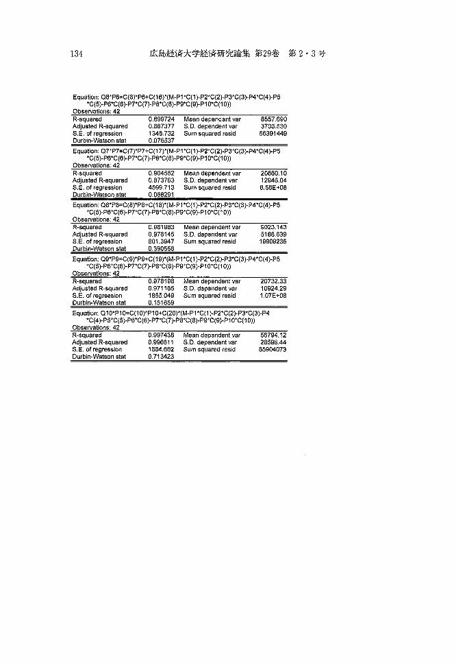
Equation: Q6*P6=C(6)*P6+C(16)*(M-P1*C(1 )-P2*C(2)-P3*C(3)-P4*C(4 )-P5 *C(5)-P6*C(6)-P7*C(7)-P8*C(8)-P9*C(9)-P1 0*C(1 0))


0.899724 0.867377 1348.732 0.076537


6557.690 3703.530

56391449

Equation: Q7*P7=C(7)*P7+C(17)*(M-P1*C(1)-P2*C(2)-P3*C(3)-P4*C(4)-P5 *C(5)-P6*C(6)-P7*C(7)-P8*C(8)-P9*C(9)-P1 0*C(1 0))


0.904552 0.873763 4599.713 0.068291


20660.10 12946.04 6.56E+08

Equation: Q8*P8=C(8)*P8+C(18)*(M-P1*C(1 )-P2*C(2)-P3*C(3)-P4*C(4 )-P5 *C(5)-P6*C(6)-P7*C(7)-P8*C(8)-P9*C(9)-P1 0*C(1 0))



9023.143 5188.639 19909236

Equation: Q9*P9=C(9 )*P9+C( 19)*(M-P1*C( 1 )-P2*C(2)-P3*C(3)-P4 *C( 4 )-P5 *C(5)-P6*C(6)-P7*C(7)-P8*C(8)-P9*C(9)-P1 0*C(1 0))


0.978198 0.971165 1855.049 0.151659


20732.33 10924.29 1.07E+08

Equation: Q1 0*P1 0=C(1 0)*P1 0+C(20)*(M-P1*C(1 )-P2*C(2)-P3*C(3)-P4 *C( 4)-P5*C( 5)-P6*C(6)-P7*C(7)-P8*C(8)-P9*C(9)-P1 O*C( 1 0))


0.997438 0.996611 1664.662 0.713423

Mean dependent var S.D. dependent var Sum squared resid

56794.12 28596.44 85904073


Appendix: Estimation ofLES model on Living Expenditure (Japan: Worker

Household)

Estimation Method: Iterative Seemingly Unrelated Regression Sample: 19632004 Simultaneous weighting matrix & coefficient iteration Convergence achieved after: 182 weight matrices, 183 total coef

iterations


C(1) 30.12914 1.443349 20.87447 0.0000 C(11) 0.159825 0.009160 17.44780 0.0000 C(2) 2.127116 0.268021 7.936365 0.0000 C(3) 4.406852 0.484444 9.096718 0.0000 C(4) 2.231857 0.149199 14.95893 0.0000 C(5) 3.338788 1.904799 1.752830 0.0804 C(6) 8.367445 0.504365 16.59005 0.0000 C(7) 15.21961 1.041232 14.61693 0.0000 C(8) 23.64671 2.465731 9.590142 0.0000 C(9) 13.12788 0.949276 13.82935 0.0000

C(10) 1.894845 1.874412 1.010901 0.3127 C(12) 0.025640 0.009217 2.782005 0.0057 C(13) 0.032139 0.006734 4.772926 0.0000 C(14) 0.039869 0.001916 20.80636 0.0000 C(15) 0.092085 0.007918 11.63033 0.0000 C(16) 0.018334 0.002016 9.093137 0.0000 C(17) 0.071557 0.010444 6.851537 0.0000 C(18) 0.049079 0.004059 12.09011 0.0000 C(19) 0.081227 0.005435 14.94490 0.0000 C(20) 0.431541 0.010056 42.91409 0.0000


Equation: Q1*P1 =C(1 )*P1 +C(11 )*(M-P1*C(1)-P2*C(2)-P3*C(3)-P4*C(4)-P5 *C( 5)-P6*C(6)-P7*C(7)-P8*C(8)-P9*C(9)-P1 0*C(1 0»



59040.74 23432.43 9.65E+08

Equation: Q2*P2=C(2)*P2+C(12)*(M-P1*C(1)-P2*C(2)-P3*C(3)-P4*C(4)-P5 *C(5)-P6*C(6)-P7*C(7)-P8*C(8)-P9*C(9)-P1 0*C(1 0»


0.942870 0.924440 2038.088 0.367242


13303.00 7414.442 1.29E+08



0.956955 0.943069 1716.049 0.373301


12759.76 7192.120

91289531

Equation: Q4*P4=C(4 )*P4+C(14 )*(M-P1*C(1 )-P2*C(2)-P3*C(3)-P4*C(4 )-P5 *C(5)-P6*C(6)-P7*C(7)-P8*C(8)-P9*C(9)-P1 0*C(1 0»


0.968221 0.957970 775.6717 1.056354


9529.976 3783.543 18651662

Equation: Q5*P5=C(5)*P5+C(15)*(M-P1*C(1 )-P2'C(2)-P3*C(3)-P4*C(4)-P5 *C(5)-P6*C(6)-P7*C(7)-P8*C(8)-P9*C(9)-P1 0'C(1 0»

Observations: 42 R-squared Adjusted R-squared S.E. of regression

0.682316 0.579837 3955.219


15840.24 6101.853 4.85E+08

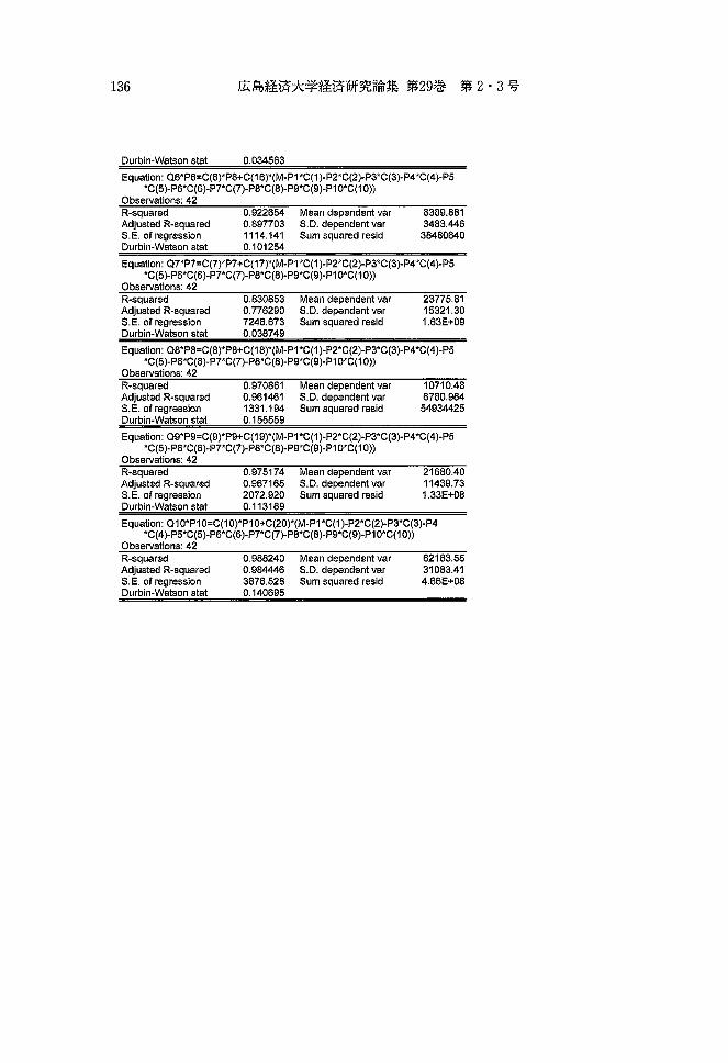
136

Durbin-Watson stat 0.034563




6389.881 3483.446 38480640

Equation: Q7*P7=C(7)*P7+C(17)*(M-P1*C(1)-P2*C(2)-P3*C(3)-P4*C(4)-P5 *C( 5 )-P6*C(6)-P7*C(7)-P8*C(8)-P9*C(9)-P1 O*C( 1 0»



23775.81 15321.30 1.63E+09

Equation: Q8*P8=C(8)*P8+C(18)*(M-P1*C(1 )-P2*C(2)-P3*C(3)-P4*C(4 )-P5 *C( 5 )-P6*C(6)-P7*C(7)-P8*C(8)-P9*C(9)-P1 O*C( 10»



10710.48 6780.964

54934425

Equation: Q9*P9=C(9)*P9+C(19)*(M-P1*C(1 )-P2*C(2)-P3*C(3)-P4*C(4)-P5 *C(5)-P6*C(6)-P7*C(7)-P8*C(8)-P9*C(9)-P1 0*C(1 0»



21680.40 11439.73 1.33E+08

Equation: Q1 0*P1 0=C(1 0)*P1 0+C(20)*(M-P1*C(1 )-P2*C(2)-P3*C(3)-P4 *C(4 )-P5*C( 5)-P6*C(6)-P7*C(7)-P8*C(8)-P9*C(9)-P1 O*C( 1 0»


0.988240 0.964446 3876.528 0.140695


62163.55 31083.41 4.66E+08

Demand Estimation and Household's Welfare...

Documents

Transcript of Demand Estimation and Household's Welfare...