ESTIMATION OF THE IMPACT OF RURAL ROADS … · ESTIMATION OF THE IMPACT OF RURAL ROADS ON HOUSEHOLD...

Asia-Pacific Development Journal Vol. 18, No. 2, December 2011

105

ESTIMATION OF THE IMPACT OF RURAL ROADSON HOUSEHOLD WELFARE IN VIET NAM

Nguyen Viet Cuong*

There is a consensus on the importance of rural roads when increasingeconomic growth and household welfare. However, little is knownregarding the positive effect these roads will have on the welfare ofhouseholds in Viet Nam. This paper aims to measure that effect. It isknown that rural roads help households increase per capita income andworking hours. The estimated impact of these roads on expenditure, theshare of non-farm income, and children’s schooling rate is not statisticallysignificant.

JEL Classification: O12, O22, R20.

Key words: Rural roads, impact evaluation, household welfare, household survey,Viet Nam.

I. INTRODUCTION

Rural roads play a crucial role in the socio-economic development of ruralareas (WB, 1994; Gannon and Liu, 1997; Lipton and Ravallion, 1995; Jalan andRavallion, 2001). Jalan and Ravallion (2001) pointed out that rural roads area necessary element for fostering rural income growth and reducing poverty. Ruralroads can increase household income, including both farm and non-farm income.They increase agricultural productivity by reducing transportation costs, increasingaccess to advanced technology, increasing capital and enabling the employment oflabour from outside local areas. Farmers also have better access to a greater numberof markets, which facilitates the selling of goods. In addition, rural roads can alsoincrease non-farm production and non-farm employment opportunities for local

* Researcher, Institute of Public Policy and Management, National Economics University, Hanoi,Viet Nam, E-mail: [email protected]. Acknowledgement: The author would like to thank the twoanonymous reviewers of the Asia-Pacific Development Journal, whose useful comments and suggestionsgreatly assisted in the preparation of this paper.


106

people. Increased income leads to an increase in consumption expenditure anda reduction in poverty. Additionally, rural roads result in an increased education levelfor children as the availability of a reliable road system reduces education costs andimproves travel to and from schools.

There are several studies that measure the impact of roads on householdwelfare. Most find a positive connection between rural roads and non-farm income.Kwon (2000) found that in Indonesia economic growth has a larger effect on povertyreduction in areas with good roads. Roads are also found to have a positive effect onwage and employment. According to Balisacan and others (2002), roads havea remarkable direct and indirect effect on the welfare of the poor in the Philippines.Fan and others (2002) examined the effect of a variety of infrastructure projects onpoverty reduction in China. They found that the effect of rural roads on povertyreduction is larger than the effect of other infrastructures. Other positive effects ofroads on household income are found in Nicaragua and Peru (Corral and Reardon,2001; Escobal, 2001).1

Viet Nam is a developing country with more than two-thirds of the populationliving in rural areas. Although Viet Nam is very successful in promoting economicgrowth and reducing poverty, poverty remains very high in rural areas, especially inthe mountain regions. In 2006, 20 per cent of the poverty stricken population of VietNam lived in rural areas, while 36 per cent resided in the Northern mountainousregions (Viet Nam, 2006). State and international agencies work continuously toimprove and maintain infrastructures, including roads. According to Donnges andothers (2007), Viet Nam had a rural road network consisting of approximately175,000 kilometres in 2007. Around 80 per cent of the population has access to anall-weather road (according to Viet Nam Household Living Standard Survey in 2006).This all-weather road can reach about 84 per cent of all rural cities and villages. Inaddition, nearly 54 per cent of provincial roads and 21 per cent of district roads arepaved (Donnges and others, 2007).

The importance of rural roads in economic growth and household welfare isclear. However, there is little specific information regarding their impact uponhousehold welfare in Viet Nam. Their impact on living standards is often mentioned inqualitative studies. Perhaps the two exceptions are Van de Walle and Cratty (2002)and Mu and Van de Walle (2007), who examined the effect of rural road rehabilitationprojects on household welfares using data collected from the projects. They foundthat rural roads improve transportation to and from local markets in Viet Nam.

1 A review on empirical studies of the impact of rural roads can be found in Ali and Pernia (2003).


107

This paper particularly investigates the impact of rural roads on householdwelfare in Viet Nam. Welfare indicators include household income and consumptionexpenditure, working effort, non-farm income and the education rate and level ofchildren. Unlike Van de Walle and Cratty (2002) and Mu and Van de Walle (2007), whomeasured the effect of specific road projects, this paper examines the effect of roadsin rural Viet Nam using nationally representative data from Viet Nam Household LivingStandard Surveys (VHLSSs) of 2004 and 2006. Therefore, estimates can berepresentative for the rural areas. In addition, the data sets used in this study aremore recent than those used by Van de Walle and Cratty (2002) and by Mu and Vande Walle (2007) (who used data surveys before 2000). The condition and effect ofa road system can change remarkably over time. Therefore, more recent data arerequired for capturing the current effect of rural roads. Two estimation methodsemployed in this study include fixed-effect regressions and difference-in-differenceswith propensity score matching, using panel data from VHLSSs 2004 and 2006.

The paper is structured into six sections. Section II introduces the data setsthat were used in this analysis. Section III presents the definition of rural roads anddiscusses their availability in Viet Nam. Section IV presents estimation methods.Estimation results are presented in section V, showing the impact assessment of ruralroads on household welfare. Finally, section VI provides the paper’s conclusion.

II. DATA SOURCE

This study relies on data from the Viet Nam Household Living StandardSurveys (VHLSSs) conducted in 2004 and 2006 by the General Statistics Office (GSO)of Viet Nam. The surveys contain household data which include basic demography,employment and labour force participation, education, health, income, expenditure,housing, fixed assets and durable goods, participation of households in povertyalleviation programs, and especially information on access to different sources ofwater for drinking and daily use. The surveys also contain commune data, whichconsist of demography and general situation of communes, general economicconditions and aid programs, non-farm employment, agriculture production, localinfrastructure and transportation, education, health, and social affairs. Communedata can be merged with household data.

The samples of the 2004 and 2006 VHLSSs covered 9,188 and 9,189households respectively. Information on commune characteristics was collectedfrom 2,181 rural communes and was representative of the urban and rural areas ofeight regions. The two surveys set up a panel data set of 4,216 households. Thispaper focuses on 3,204 of those households, which belong to 1,068 communes. Itshould be noted that in VHLSS, each village is sampled from each commune.


108

Therefore, the number of villages in this sample is also 1,068, and there are 3households per village.

III. RURAL ROADS IN VIET NAM

Viet Nam has a highly dense population. The country is approximately331,688 square kilometres in size, but had a population of nearly 86 million in 2009.Currently, Viet Nam is divided into 63 provinces, with each province further dividedinto districts. Smaller administrative units are called communes and villages. In2009, there were 685 districts, 10,987 communes, and 125,710 villages. The averagepopulation of a village is around 685. In 2006, 97 per cent of rural communescontained an internal road that was passable by cars. However, the proportion ofvillages that could be reached by cars, in other words, having a connecting road thatwas passable by cars was lower. The proportion of households living in rural villageswith a road which could be driven year round was 72.8 per cent in 2004 and 79.7 percent in 2006 (see figure 1).2

Figure 1. Percentage of households living in villages with a good road

2 In the VHLSSs, there is a question: ‘For how many months during the past year was the roadpassable by cars?’ The answers are coded from 1 month to 12 months. In this study, we define a villagehaving a good road if the road is passable for 12 months.

Source: Author’s estimation from VHLSSs 2004 and 2006.

66.0

72.8

82.9 81.5

70.3

79.7

74.9

59.9

74.7

60.2

0

20

40

60

80

100

Kinh/Hoa Ethnic minorities Non-poor Poor All rural

2004 2006


109

Although the proportion of people living in a village with a good roadincreased between 2004-2006, there was still a large disparity in accessing a roadbetween different groups (figure 1). In 2006, the proportion of households living ina village with access to a good road was 82.9 per cent for Kinh and Hoa and 60.2 percent for ethnic minorities. The figure for the non-poor and the poor was 81.5 per centand 70.3 per cent respectively. It should be noted that while the percentage of peopleaccessing a road in villages increases for all household groups, the differencebetween the poor and the non-poor as well as the Kinh/Hoa and ethnic minorityhouseholds tended to be larger between 2004 and 2006.

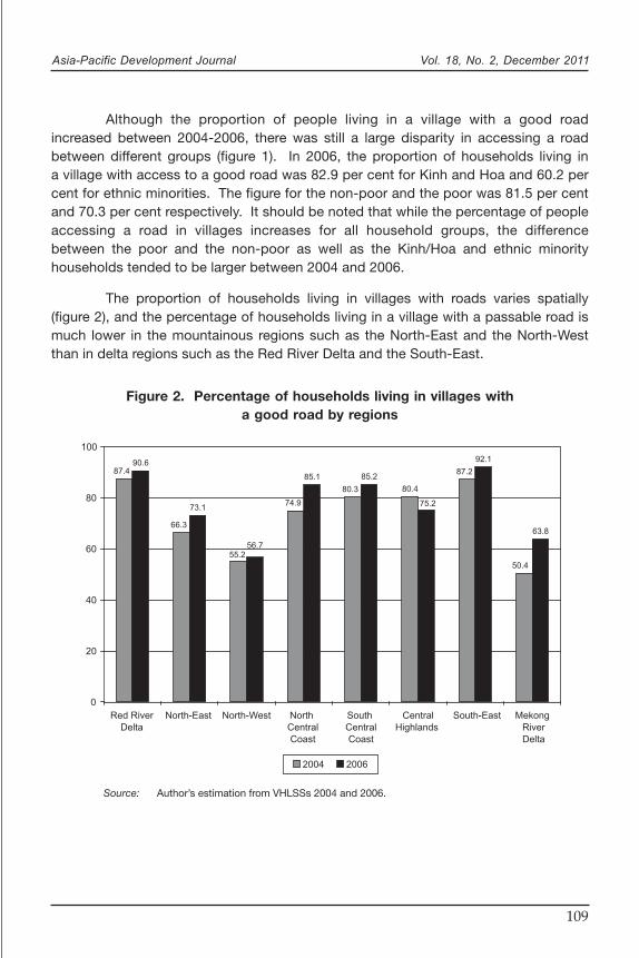
The proportion of households living in villages with roads varies spatially(figure 2), and the percentage of households living in a village with a passable road ismuch lower in the mountainous regions such as the North-East and the North-Westthan in delta regions such as the Red River Delta and the South-East.

Figure 2. Percentage of households living in villages witha good road by regions


87.4

66.3

55.2

74.9

80.3 80.4

87.2

50.4

90.6

73.1

56.7

85.1 85.2

75.2

92.1

63.8

0

20

40

60

80

100

Red River

Delta

North-East North-West North

Central

Coast

South

Central

Coast

Central

Highlands

South-East Mekong

River

Delta

2004 2006


110

IV. ESTIMATION METHOD

In this study, we use two methods to estimate the effect of rural roads onhousehold welfare. This section describes these methods.

Fixed-effects regression

We use a similar specification for estimating the effect of rural roads on percapita income, per capita expenditure, work efforts, the share of non-farm income,and on children’s education enrollment:

Yijt

= β0 + X

ijtβ

1 + D

jtβ

2 + C

jtβ

3 + u

ij + v

j + ε

ijt, t = 1, 2 (1)

Where Y is a vector including income per capita, expenditure per capita, and otherhousehold welfare indicators, the subscripts i, j and t refer to household i in village j attime t respectively. X is a vector of household variables. D is a dummy variableindicating whether a village has a good road. C is a vector of control variables withvillage characteristics. u

ij and v

j are unobserved time-invariant household and village

characteristics respectively. εijt is an error term. The summary statistics of dependent

and independent variables is presented in annex tables A.1 and A.2. The impact ofavailability of a rural road in a village on household welfare is measured by β

2.

A common problem during an impact evaluation of rural households is theendogeneity of roads (Van de Walle, 2002). Households in an area with a largenumber of roads obviously have better conditions. It is more difficult to separate theeffect of rural roads from the effect of other unobserved simultaneous factors at work.Technically, unobserved variables in regressions are correlated with rural roads. Astandard method to deal with the endogeneity is instrumental variables regression.However, finding a valid instrument which is correlated with rural roads but nothousehold welfare is a difficult task. We tried a variable of historic road network asthe instrument for current rural roads, but this instrument does not work. Therefore, inthis study we use fixed-effects regressions to estimate equation number 1. In fixed-effects regressions, the time invariant household and commune characteristics,including u

ij and v

j which are correlated with the rural road, are dropped from the

model. It is expected that unobserved variables which are time-variant are notcorrelated with rural roads in the household welfare equation.

Time-invariant observed variables, like regional dummies, are also removedin fixed-effects regressions. To control time-invariant variables, we can interact thesetime-invariant observed variables with other time-variant observed variables andcontrol these interactions in the fixed-effects regression.


111

Difference-in-differences with propensity score matching

In addition to the fixed-effects regrssions, we also used the difference-in-differences with propensity score matching. This method is ideally applied toevaluate the impact of a program when we have data on the treatment and controlbefore and after the program implementation. For the impact of rural roads, the 2004VHLSS was not clean baseline data since there were many households living invillages with a good road in 2004. In addition, there were a number of households ina village in which there was a good road in 2004 but not in 2006 due to thedeterioration of road quality. To apply the difference-in-differences estimator, welimited our sample to households who lived in a village without a good road in 2004.This sample consisted of 686 households, of these households there were 281households living in villages with a good road in 2006 and 405 households living invillages without a good road in 2006. The 281 households set up the treatmentgroup, while the 405 households set up the control group.

These control and treatment groups can be used to measure the effect ofrural roads. The difference-in-differences estimator can be expressed as follows:

ATT = (YT2006 – Y

C2006 ) – (YT

2004 – YC

2004 ), (2)

where YT

2004 and YC

2004 is the mean of a welfare indicator of interest of the treatmentgroup (households living in villages with a good road in 2006) and the control group(households living in villages without a good road in 2006) in the year 2004respectively. Y

T2006 and Y

C2006 are the welfare means of the treatment group and the

control group in 2006 respectively.

The above parameter of the program impact is Average Treatment Effect onthe Treated, which is most popular parameter in impact evaluation (Heckman andothers, 1999). This is the expected impact of the rural roads on the treatment group.To remove the difference in welfare between the treatment and control groups, due toobserved variables, we combined the difference-in-differences estimator withpropensity score matching. The control group was constructed in a way so that it issimilar to the treatment group. In order to construct a comparison group that wassimilar to the treatment group in observed characteristics, matched each household inthe treatment group (participants) with households in the control group (non-participants) based on the similarity of observed characteristics. There were a largenumber of characteristic variables and finding “close” non-participants to match witha participant was not straightforward. A widely-used way to find the matched sampleis the propensity score matching, which is the probability of being assigned into theprogram (Rosenbaum and Rubin, 1983). In this study, the matching based on the

ˆ


112

propensity score is proposed to be employed.3 The propensity score is oftenestimated using a probit or logit regression. Once the scores are estimated,participants are matched with non-participants according to the closeness ofestimated scores. Standard errors of the estimator given by equation (2) can beestimated using bootstrap.

Compared with the fixed-effects regressions, the difference-in-differenceswith propensity score matching has an advantage in that it does not rely on theassumption of the functional form of welfare outcomes. However, in this study sincewe restricted our sample when using the difference-in-differences with propensityscore matching, estimates from this method should be interpreted for this restrictedsample, not for the entire population.

V. ESTIMATION RESULTS

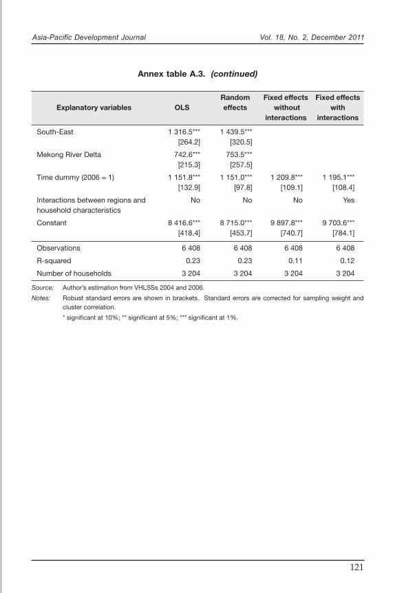
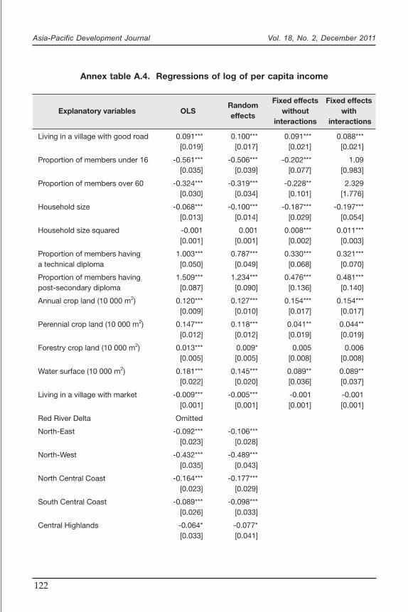
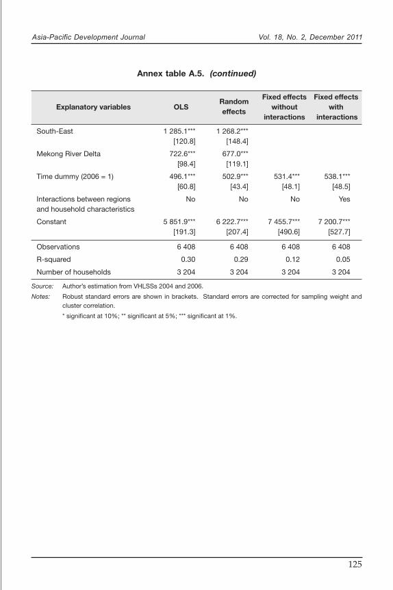
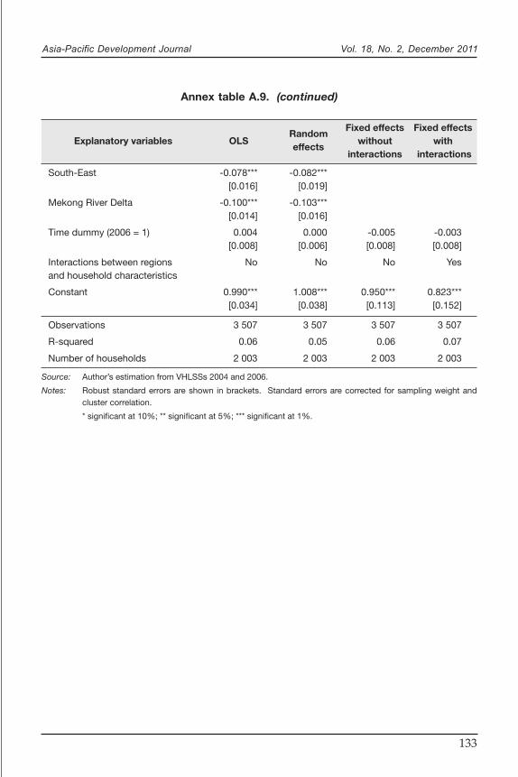
Table 1 presents the coefficient of rural roads in regressions of differenthousehold welfare indicators. Four models were used: ordinary least squares (OLS),random-effects, fixed-effects without and fixed-effects with interactions betweenregional dummies and household demographic variables. OLS and random-effectsmodels are presented for comparison and examination of potential biases caused byunobserved time-invariant variables. For income and expenditure, in addition to linearmodels presented by equation number 1, we also use semi-log functions. Table 1reports only the estimates of rural roads, and the full regressions are reported inannex tables A.3 to A.9.

It shows that rural roads have a positive effect on household income. Theestimates of the impact on income are quite similar in different models. According tofixed-effect linear regression with interactions, rural roads increase per capita incomeby around VND4 858,000. The fixed-effect regressions log of per capita incomeindicates an increase of approximately 8.8 per cent. It should be noted that incomeand expenditure of 2004 are adjusted to reflect those of 2006.

The impact on per capita expenditure is positive, but not statisticallysignificant in fixed-effect regressions. The point estimate of the impact onexpenditure is much lower than the estimate on income. It implies that rural roadshave positive effects on households’ investment and saving. In addition, expenditureis less fluctuated than income. Houeseholds with low income still have to keep

3 Other matching methods can be subclassification (see, e.g., Cochran and Chambers, 1965;Cochran, 1968) and covariate matching (Rubin, 1978; 1979).

4 Viet Nam Dong.


113

Table 1. The estimates of the impact of rural using regressions

Regression models

Dependent variables Fixed Fixed

(outcome variables) OLSRandom effects effectseffects without with

interactions interactions

Per capita income (thousand VND) 527.6*** 666.3*** 867.2*** 858.0***[189.4] [183.7] [273.8] [278.4]

Log of per capita income 0.091*** 0.100*** 0.091*** 0.088***(thousand VND) [0.019] [0.017] [0.021] [0.021]

Per capita expenditure (thousand VND) 227.3*** 228.9*** 205.4 214.4[86.6] [82.9] [144.0] [146.8]

Log of per capita expenditure 0.056*** 0.042*** 0.014 0.014(thousand VND) [0.016] [0.014] [0.019] [0.019]

Annual working hours per capita 40.28*** 38.02*** 34.34* 37.13**[14.02] [13.76] [18.69] [18.84]

The share of non-farm income 0.040*** 0.023*** 0.004 0.002[0.010] [0.009] [0.010] [0.010]

Proportion of children attending school 0.010 0.001 0.002 -0.025[0.011] [0.011] [0.020] [0.020]


Notes: In fixed-effects models with interactions, we interacted regional dummies with three demographicvariables of households, including size, proportion of members under 16 and proportion of membersover 60. There are 21 interaction terms controlled in the fixed-effects models.

Income and expenditure data of the 2004 VHLSS are deflated to the 2006 price for comparison.

Robust standard errors are shown in brackets. Standard errors are corrected for sampling weight andcluster correlation.

* significant at 10%; ** significant at 5%; *** significant at 1%.

consumption expenditure at a sufficient level. Thus, rural roads can have a minimalimpact on expenditure.

Households in a village with a good road are more likely to have higherworking hours per person than those without one. Although the effect estimated ataround 37 hour per person per year is small, it implies the importance of rural roads inincreasing employment. The effect of rural roads on the share of non-farm income intotal household income and the schooling rate of children between the ages of 6 and17 is not statistically significant.


114

As mentioned in section III, most communes have a road which leads to thecommune center. The impact of a village road can depend on the closeness ofa village to its commune road. In the VHLSS, we did not have data on the distance.Although the distance between village and commune road can increase or mitigatethe actual effect of the road, it does not make our estimate biased as the distancefrom village to commune road is assumed to be fixed during the time of the study,2004 to 2006, and can therefore be eliminated by the fixed-effects regressions.

The second method to measure the impact of rural roads is the difference-in-differences with propensity score matching. The first step is to predict a propensityscore using a probit regression. Annex table A.10 presents this regression. Thedependent variable is a binary one indicating whether or not a household lived ina village with a good road in 2006. The explanatory variables are the characteristicsof households in 2004. The estimated propensity score is presented in annex figureA.1, which indicates a large common support between the treatment and controlgroups. It means that we were able to select similar households from the controlgroup to match households in the treatment group.

The second step is to construct the control group. Depending on thenumber of non-participants matched with participants, there can be nearest-neighbours matching and kernel matching. Since standard errors computed bybootstrap can be invalid for the nearest-neighbours macthing (Abadie and Imbens,2006), we used kernel matching with a bandwidth of 0.05. Kernel matching, usingother bandwidths such as 0.01 and 0.03, produces similar estimates, but they are notrepresented here. Table 2 presents the estimates from the difference-in-differenceswith propensity score matching. It shows very similar estimates as the fixed-effectsregressions. Living in a village with a good road can increase household income andworking hours. The effect on consumption and child education is positive, but notstatistically significant.

VI. CONCLUSIONS

Viet Nam has achieved remarkable economic growth and poverty reductionover the past 20 years, with the average annual rate of economic growth ofapproximately 7 per cent. The poverty rate decreased from 58 per cent in 1993 to37 per cent in 1998 and then to 16 per cent in 2006. Household living standards havebeen also steadily improved. Infrastructures, especially roads, have been playingimportant roles in increasing household welfare in Viet Nam. Using VHLSS data, thispaper makes an effort to estimate the impact of rural roads on household welfare andshows that they have a positive effect on household income. Rural roads increaseper capita income by around VND 858,000, or equivalently 8.8 per cent of mean


115

income. However, the impact on per capita expenditure is much lower. Theestimated amount is positive, but not statistically significant in fixed-effectregressions. It implies that rural roads have positive effects on households’investment and saving. It is interesting that households living in a village with a goodroad are more likely to have longer working hours per person than households living ina village without a rural road. The effects of rural roads on the percentage of non-farm income or level of education in total household income are not statisticallysignificant.

The findings suggest several policy implications for Viet Nam. As noted, ruralroads are an important factor for economic growth. At the household level theyincrease employment and income. Thus, policies geared towards improvinghousehold access to these roads are important. However, at least in the short-term arural road policy is not effective in reducing poverty if said poverty is measured basedon a consumption indicator. Finally, roads are not effective at increasing the share ofnon-farm income and the level of education. The implication is that improving ruralroads simply increases access of people to public services and markets. Improvingrural roads alone is not enough as other infrastructres, such as markets and schools,need to be upgraded.

Table 2. The estimates of the impact of rural using diffference-in-differenceswith propensity score matching (kernel matching with bandwidth of 0.05)

Dependent variables 2004 2006Diff-in-diff

(outcome variables) Treatment Control Diff Treatment Control Diff

(1) (2) (3)=(1)-(2) (4) (5) (6)=(4)-(5) (7)=(6)-(3)

Per capita income 5 619.0*** 4 758.4*** 860.6** 7 454.0*** 5 739.5*** 1 714.6*** 854.0**(thousand VND) [306.9] [176.4] [347.8] [552.6] [210.0] [568.4] [422.6]

Per capita expenditure 4 032.9*** 3 327.3*** 705.6*** 4 770.1*** 3 862.9*** 907.1*** 201.5(thousand VND) [169.5] [112.8] [211.4] [214.8] [104.1] [364.4] [140.6]

Annual working hours 865.4*** 946.0*** -80.6* 912.3*** 919.6*** -7.3 73.3*per capita [26.7] [30.7] [43.1] [30.3] [29.7] [45.2] [42.1]

The share of 0.316*** 0.326*** -0.010 0.321*** 0.333*** -0.011 -0.001non-farm income [0.019] [0.019] [0.023] [0.018] [0.019] [0.021] [0.019]

Proportion of children 0.484*** 0.475*** 0.010 0.451*** 0.439*** 0.011 0.002

attending school [0.030] [0.029] [0.020] [0.029] [0.029] [0.022] [0.014]

Notes: (i) Income and expenditure data of the 2004 VHLSS are deflated to the 2006 price for comparison.

(ii) Standard errors are indicated by brackets and are calculated using bootstrap with 500 replications.



116

REFERENCES

Abadie, A. and G.W. Imbens (2006). “On the failure of the bootstrap for matching estimators”,Technical Working Paper No. 325 (New York, National Bureau of Economic Research).

Ali, I. and E.M. Pernia (2003). “Infrastructure and poverty reduction. What is the connection?”, ERDPolicy Brief No. 13 (Manila, Asian Development Bank).

Balisacan, A.M., E.M. Pernia and A. Asra (2002). “Revisiting growth and poverty reduction inIndonesia: what do subnational data show?”, ERD Working Paper Series No. 25,Economics and Research Department (Manila, Asian Development Bank).

Cochran, W.G. (1968). “The effectiveness of adjustment by subclassification in removing bias inobservational studies”, Biometrics, vol. 24, No. 2, pp. 295-313.

Cochran, W.G. and S. Paul Chambers (1965). “The planning of observational studies of humanpopulation”, Journal of the Royal Statistical Society, vol. 128 No. 2, pp. 234-266.

Corral, L. and T. Reardon (2001). “Rural nonfarm incomes in Nicaragua”, World Development, vol. 29,No. 3, pp. 427-442.

Donnges, Ch., G. Edmonds and B. Johannessen (2007). Rural Road Maintenance – Sustaining theBenefits of Improved Access (Bangkok, International Labour Office).

Escobal, J. (2001). “The determinants of nonfarm income diversification in rural Peru”, WorldDevelopment, vol. 29, No. 3, pp. 497-508.

Fan, S., L.X. Zhang and X.B. Zhang (2002). “Growth, inequality, and poverty in rural China: the role ofpublic investments”, Research Report 125 (Washington, D.C., International Food PolicyResearch Institute).

Gannon, C. and Z. Liu (1997). “Poverty and transport”, TWU discussion papers, TWU-30(Washington, D.C., World Bank).

Heckman, J., R. Lalonde and J. Smith (1999). “The economics and econometrics of active labourmarket programs”, Handbook of Labour Economics, Volume 3, A. Ashenfelter andD. Card, eds. (Amsterdam, Elsevier Science).

Jalan, J. and M. Ravallion (2001). “Geographic poverty traps? A micro econometric model ofconsumption growth in rural China”, Journal of Applied Econometrics, vol. 17, No. 4,pp. 329-346.

Kwon, E.K. (2000). “Infrastructure, growth, and poverty reduction in Indonesia: a cross – sectionalanalysis”, paper presented at the Asian Development Bank’s Transport Infrastructure andPoverty Reduction Workshop, Manila, 18-22 July 2005.

Lipton, M. and M. Ravallion (1995). “Poverty and policy”, in J. Behrman and T. N. Srinivasan, eds.,Handbook of Development Economics (Handbooks in Economics 9), vol. 3B , pp. 2551-2657 (Amsterdam, Elsevier Science).

Mu, R. and D. Van de Walle (2007). “Rural roads and local market development in Viet Nam”, PolicyResearch Working Paper No. 4340 (Washington, D.C., World Bank).

Rosenbaum, P. and R. Rubin (1983). “The central role of the propensity score in observational studiesfor causal effects”, Biometrika, vol. 70, No. 1, pp. 41-55.

Rubin, Donald (1978). “Bayesian inference for causal effects: the role of randomization”, The Annalsof Statistics, vol. 6, No. 1, pp. 34-58.


117

Rubin, Donald B. (1979). “Using multivariate sampling and regression adjustment to control bias inobservational studies”, Journal of the American Statistical Association, vol. 74, No. 366,pp. 318-328.

Van de Walle, D. (2002). “Choosing rural road investments to help reduce poverty”, WorldDevelopment, vol. 30, No. 4, pp. 575-589.

Van de Walle, D. and D. Cratty (2002). “Impact evaluation of a rural road rehabilitation project”, reportof a World Bank project on rural road rehabilitation in Viet Nam.

World Bank (WB) (1994). World Development Report 1994: Infrastructure for Development(New York, Oxford University Press).


118

APPENDIX

Annex table A.1. Summary statistics of variables in 2004

Households living in Households living in

Variablea village with a village without

Type good road good road

Mean Std. Dev. Mean Std. Dev.

Per capita income (thousand VND) Continuous 5 892.3 4 983.9 5 382.4 4 744.3Per capita expenditure Continuous 4 231.8 2 709.8 3 846.0 2 756.8(thousand VND)

Annual working hours per capita Continuous 923.1 507.3 868.5 462.6

Proportion of non-farm income Continuous 0.3859 0.3197 0.3120 0.3200

Proportion of children attending Continuous 0.5246 0.4920 0.5395 0.4850school

Household size Continuous 4.3487 1.6931 4.6653 1.8194

Proportion of members under 16 Continuous 0.2553 0.2192 0.2688 0.2147

Proportion of members over 60 Continuous 0.1262 0.2578 0.1083 0.2285

Proportion of members having Continuous 0.0524 0.1386 0.0312 0.1146technical diploma

Proportion of members having Continuous 0.0157 0.0785 0.0080 0.0553post-secondary diploma

Annual crop land (10 000m2) Continuous 0.3581 0.6324 0.5416 0.8524

Perennial crop land (10 000m2) Continuous 0.1281 0.6440 0.1159 0.5298

Forestry crop land (10 000m2) Continuous 0.0955 0.6055 0.2776 2.0903

Water surface (10 000m2) Continuous 0.0134 0.1255 0.0717 0.3794

Living in a village with market Dummy 2.5283 4.4057 4.3043 8.7499

Red River Delta Dummy 0.2700 0.4441 0.0903 0.2868

North-East Dummy 0.1441 0.3512 0.1817 0.3858

North-West Dummy 0.0354 0.1847 0.0850 0.2791

North Central Coast Dummy 0.1233 0.3288 0.1360 0.3430

South Central Coast Dummy 0.0990 0.2987 0.0584 0.2347

Central Highlands Dummy 0.0645 0.2457 0.0393 0.1945

South-East Dummy 0.1140 0.3179 0.0436 0.2042

Mekong River Delta Dummy 0.1498 0.3570 0.3656 0.4818

Number of observations 2 263 941


Note: Income and expenditure data of the 2004 VHLSS are deflated to the 2006 price for comparison.


119

Annex table A.2. Summary statistics of variables in 2006

Households living in Households living in

Variablea village with a village without

Type good road good road

Mean Std. Dev. Mean Std. Dev.

Per capita income (thousand VND) Continuous 7 383.2 7 209.3 6 407.9 5 461.9

Per capita expenditure Continuous 4 917.9 3 042.9 4 268.3 2 652.0(thousand VND)

Annual working hours per capita Continuous 947.2 530.5 894.6 517.8

Proportion of non-farm income Continuous 0.4048 0.3326 0.2959 0.3072

Proportion of children attending Continuous 0.4841 0.4946 0.4770 0.4868school

Household size Continuous 4.2343 1.6534 4.6657 1.9128

Proportion of members under 16 Continuous 0.2237 0.2106 0.2459 0.2150

Proportion of members over 60 Continuous 0.1346 0.2666 0.1208 0.2417

Proportion of members having Continuous 0.0561 0.1438 0.0333 0.1150technical diploma

Proportion of members having Continuous 0.0160 0.0802 0.0107 0.0719post-secondary diploma

Annual crop land (10 000m2) Continuous 0.3765 0.7608 0.6339 0.9231

Perennial crop land (10 000m2) Continuous 0.1322 0.5624 0.1588 0.6150

Forestry crop land (10 000m2) Continuous 0.1478 1.3430 0.3138 2.0670

Water surface (10 000m2) Continuous 0.0252 0.3463 0.0750 0.3942

Living in a village with market Dummy 2.5423 4.3902 5.8114 12.9226

Red River Delta Dummy 0.2535 0.4351 0.0882 0.2838

North-East Dummy 0.1431 0.3503 0.1977 0.3986

North-West Dummy 0.0340 0.1812 0.1067 0.3089

North Central Coast Dummy 0.1379 0.3449 0.0882 0.2838

South Central Coast Dummy 0.0952 0.2935 0.0583 0.2345

Central Highlands Dummy 0.0560 0.2299 0.0612 0.2398

South-East Dummy 0.1100 0.3129 0.0341 0.1817

Mekong River Delta Dummy 0.1703 0.3760 0.3656 0.4819

Number of observations 501 703


Note: Income and expenditure data of the 2004 VHLSS are deflated to the 2006 price for comparison.


120

Annex table A.3. Regressions of per capita income (thousand VND)

Random Fixed effects Fixed effectsExplanatory variables OLS effects without with


Living in a village with good road 527.6*** 666.3*** 867.2*** 858.0***[189.4] [183.7] [273.8] [278.4]

Proportion of members under 16 -2 242.8*** -2 196.9*** -521.4 7 127.70[356.6] [394.5] [1 067.6] [6 778.3]

Proportion of members over 60 -2 185.0*** -2,180.6*** -1 445.2* 28 494.6**[299.8] [343.4] [857.0] [13 281.2]

Household size -885.4*** -1 009.1*** -1 592.3*** -1 413.6**[130.5] [142.3] [270.5] [588.4]

Household size squared 24.9** 34.3*** 78.0*** 98.6***[11.5] [12.5] [20.2] [29.6]

Proportion of members having 7 904.3*** 6 707.9*** 2 827.7*** 2 696.5***a technical diploma [503.2] [516.4] [937.9] [956.2]

Proportion of members having 15 147.6*** 12 625.1*** 3 021.70 3 048.50post-secondary diploma [879.9] [933.3] [2 934.1] [2 956.7]

Annual crop land (10 000 m2) 1 524.6*** 1 548.3*** 1 776.1*** 1 818.2***[93.8] [103.0] [478.5] [492.4]

Perennial crop land (10 000 m2) 1 792.4*** 1 407.7*** -95.5 -53[116.6] [123.6] [570.7] [583.3]

Forestry crop land (10 000 m2) 113.1** 107.2** 94.9 100.3[48.1] [49.1] [112.2] [114.5]

Water surface (10 000 m2) 1 659.3*** 1 450.6*** 856.1*** 864.4***[222.0] [216.8] [266.9] [278.6]

Living in a village with market -54.1*** -36.5*** -9.5 -8.7[10.7] [10.1] [7.0] [7.3]

Red River Delta Omitted

North-East -800.7*** -834.2***[227.9] [274.8]

North-West -2 574.8*** -2 820.2***[356.8] [426.5]

North Central Coast -947.0*** -1 001.3***[235.6] [286.4]

South Central Coast -635.3** -660.0**[266.4] [324.3]

Central Highlands -1 020.4*** -897.2**[331.2] [398.6]


121

South-East 1 316.5*** 1 439.5***[264.2] [320.5]

Mekong River Delta 742.6*** 753.5***[215.3] [257.5]

Time dummy (2006 = 1) 1 151.8*** 1 151.0*** 1 209.8*** 1 195.1***[132.9] [97.8] [109.1] [108.4]

Interactions between regions and No No No Yeshousehold characteristics

Constant 8 416.6*** 8 715.0*** 9 897.8*** 9 703.6***[418.4] [453.7] [740.7] [784.1]

Observations 6 408 6 408 6 408 6 408

R-squared 0.23 0.23 0.11 0.12

Number of households 3 204 3 204 3 204 3 204


Notes: Robust standard errors are shown in brackets. Standard errors are corrected for sampling weight andcluster correlation.


Annex table A.3. (continued)

Random Fixed effects Fixed effectsExplanatory variables OLS effects without with



122

Annex table A.4. Regressions of log of per capita income

RandomFixed effects Fixed effects

Explanatory variables OLSeffects

without withinteractions interactions

Living in a village with good road 0.091*** 0.100*** 0.091*** 0.088***[0.019] [0.017] [0.021] [0.021]

Proportion of members under 16 -0.561*** -0.506*** -0.202*** 1.09[0.035] [0.039] [0.077] [0.983]

Proportion of members over 60 -0.324*** -0.319*** -0.228** 2.329[0.030] [0.034] [0.101] [1.776]

Household size -0.068*** -0.100*** -0.187*** -0.197***[0.013] [0.014] [0.029] [0.054]

Household size squared -0.001 0.001 0.008*** 0.011***[0.001] [0.001] [0.002] [0.003]

Proportion of members having 1.003*** 0.787*** 0.330*** 0.321***a technical diploma [0.050] [0.049] [0.068] [0.070]

Proportion of members having 1.509*** 1.234*** 0.476*** 0.481***post-secondary diploma [0.087] [0.090] [0.136] [0.140]

Annual crop land (10 000 m2) 0.120*** 0.127*** 0.154*** 0.154***[0.009] [0.010] [0.017] [0.017]

Perennial crop land (10 000 m2) 0.147*** 0.118*** 0.041** 0.044**[0.012] [0.012] [0.019] [0.019]

Forestry crop land (10 000 m2) 0.013*** 0.009* 0.005 0.006[0.005] [0.005] [0.008] [0.008]

Water surface (10 000 m2) 0.181*** 0.145*** 0.089** 0.089**[0.022] [0.020] [0.036] [0.037]



North-East -0.092*** -0.106***[0.023] [0.028]

North-West -0.432*** -0.489***[0.035] [0.043]

North Central Coast -0.164*** -0.177***[0.023] [0.029]

South Central Coast -0.089*** -0.098***[0.026] [0.033]

Central Highlands -0.064* -0.077*[0.033] [0.041]


123

South-East 0.170*** 0.175***[0.026] [0.033]


Time dummy (2006 = 1) 0.171*** 0.172*** 0.177*** 0.177***[0.013] [0.009] [0.009] [0.009]

Interactions between regions No No No Yesand household characteristics

Constant 8.789*** 8.867*** 9.025*** 8.983***[0.041] [0.044] [0.081] [0.085]

Observations 6 407 6 407 6 407 6 407

R-squared 0.34 0.34 0.23 0.24










124

Annex table A.5. Regressions of per capita expenditure (thousand VND)




Living in a village with good road 227.3*** 228.9*** 205.4 214.4[86.6] [82.9] [144.0] [146.8]

Proportion of members under 16 -2 462.5*** -2 321.9*** -1 182.8*** 3 675.60[163.0] [180.5] [324.1] [2 655.9]

Proportion of members over 60 -871.1*** -910.1*** -786.4 13 126.6*[137.1] [157.8] [530.4] [7 182.1]

Household size -451.5*** -554.2*** -931.9*** -982.8***[59.7] [65.0] [162.3] [306.2]

Household size squared 14.0*** 20.5*** 42.6*** 49.6***[5.3] [5.7] [13.2] [13.9]

Proportion of members having 4 664.4*** 3 545.8*** 539.3 475.8technical diploma [230.0] [234.4] [448.8] [446.9]

Proportion of members having 7 621.0*** 6 173.9*** 878.8 845.8post-secondary diploma [402.2] [425.0] [1 341.7] [1 275.8]

Annual crop land (10 000 m2) 283.5*** 258.1*** 181.0** 169.3*[42.9] [47.1] [86.6] [88.5]

Perennial crop land (10 000 m2) 435.8*** 419.5*** 326.3*** 318.5***[53.3] [56.3] [90.1] [89.8]

Forestry crop land (10 000 m2) 1.1 -15.9 -51.6*** -50.7**[22.0] [22.3] [18.7] [21.2]

Water surface (10 000 m2) 458.2*** 341.9*** 103.4 150[101.5] [97.9] [201.5] [177.4]



North-East -428.6*** -475.6***[104.2] [127.2]

North-West -1 052.9*** -1 205.2***[163.1] [197.2]


South Central Coast 74.8 34.3[121.8] [150.2]

Central Highlands -36.5 -119.5[151.4] [184.4]


125

South-East 1 285.1*** 1 268.2***[120.8] [148.4]


Time dummy (2006 = 1) 496.1*** 502.9*** 531.4*** 538.1***[60.8] [43.4] [48.1] [48.5]


Constant 5 851.9*** 6 222.7*** 7 455.7*** 7 200.7***[191.3] [207.4] [490.6] [527.7]

Observations 6 408 6 408 6 408 6 408

R-squared 0.30 0.29 0.12 0.05










126

Annex table A.6. Regressions of log of per capita expenditure





Proportion of members under 16 -0.609*** -0.556*** -0.324*** 0.753[0.030] [0.032] [0.056] [0.539]

Proportion of members over 60 -0.222*** -0.219*** -0.169** 1.966[0.025] [0.029] [0.075] [2.069]

Household size -0.053*** -0.079*** -0.135*** -0.174***[0.011] [0.012] [0.024] [0.052]

Household size squared -0.001 0.000 0.004* 0.006***[0.001] [0.001] [0.002] [0.002]

Proportion of members having 0.843*** 0.566*** 0.077 0.071technical diploma [0.042] [0.041] [0.062] [0.063]

Proportion of members having 1.226*** 0.870*** 0.074 0.052post-secondary diploma [0.073] [0.075] [0.135] [0.128]

Annual crop land (10 000 m2) 0.053*** 0.051*** 0.053*** 0.051***[0.008] [0.008] [0.014] [0.015]

Perennial crop land (10 000 m2) 0.095*** 0.082*** 0.054*** 0.053***[0.010] [0.010] [0.013] [0.014]

Forestry crop land (10 000 m2) 0.002 -0.005 -0.013*** -0.012***[0.004] [0.004] [0.003] [0.004]

Water surface (10 000 m2) 0.096*** 0.062*** 0.018 0.024[0.019] [0.017] [0.026] [0.024]

Living in a village with market -0.009*** -0.004*** 0 0.001[0.001] [0.001] [0.001] [0.001]


North-East -0.137*** -0.157***[0.019] [0.024]

North-West -0.405*** -0.469***[0.030] [0.037]


South Central Coast -0.044** -0.056*[0.022] [0.029]

Central Highlands -0.108*** -0.133***[0.028] [0.035]


127

South-East 0.186*** 0.185***[0.022] [0.028]


Time dummy (2006 = 1) 0.123*** 0.125*** 0.130*** 0.130***[0.011] [0.007] [0.007] [0.007]

Interactions between regions No No No Yesand households characteristics

Constant 8.533*** 8.629*** 8.757*** 8.710***[0.035] [0.037] [0.070] [0.072]

Observations 6 408 6 408 6 408 6 408

R-squared 0.38 0.36 0.19 0.11










128

Annex table A.7. Regressions of annual working hours per capita




Living in a village with good road 40.28*** 38.02*** 34.34* 37.13**[14.02] [13.76] [18.69] [18.84]

Proportion of members under 16 -881.6*** -852.8*** -719.9*** -414.40[26.401] [29.075] [63.226] [839.42]

Proportion of members over 60 -1 342.3*** -1 337.7*** -1 338.4*** 1 148.69[22.196] [25.177] [86.393] [1 913.6]

Household size -37.39*** -41.70*** -59.308** -109.56*[9.660] [10.508] [26.404] [62.564]

Household size squared 1.247 1.546* 2.984 5.003*[0.852] [0.923] [2.089] [2.841]

Proportion of members having 75.985** 98.613** 173.734*** 156.021**technical diploma [37.251] [38.437] [65.082] [65.494]

Proportion of members having 212.08*** 256.81*** 461.027** 434.952**post-secondary diploma [65.138] [69.181] [200.812] [193.530]

Annual crop land (10 000 m2) -18.945*** -16.449** 2.225 -3.178[6.943] [7.595] [16.086] [16.858]

Perennial crop land (10 000 m2) -7.613 -2.059 27.789** 25.863*[8.634] [9.166] [12.870] [13.469]

Forestry crop land (10 000 m2) -1.483 0.132 8.841 10.121[3.558] [3.655] [6.984] [6.808]

Water surface (10 000 m2) -1.651 22.280 77.400*** 74.405***[16.434] [16.232] [27.350] [28.738]

Living in a village with market -1.522* -1.223 -0.389 -0.326[0.794] [0.762] [1.074] [1.098]


North-East 77.163*** 74.054***[16.871] [19.984]

North-West 41.188 34.568[26.415] [31.045]


South Central Coast -54.799*** -56.339**[19.726] [23.555]

Central Highlands 11.369 4.205[24.521] [28.997]


129

South-East 58.875*** 56.229**[19.561] [23.287]

Mekong River Delta -72.26*** -74.99***[15.94] [18.74]

Time dummy (2006 = 1) 10.212 10.479 9.889 12.104[9.840] [7.506] [8.234] [8.370]


Constant 1 418.4*** 1 421.6*** 1 404.4*** 1 457.6***[30.972] [33.487] [82.036] [95.273]

Observations 6 408 6 408 6 408 6 408

R-squared 0.42 0.42 0.4 0.18


Source: Author’s estimation from VHLSSs 2004 and 2006








130

Annex table A.8. Regressions of the share of non-farm income





Proportion of members under 16 0.009 -0.029 -0.106*** -0.308[0.019] [0.020] [0.037] [0.238]

Proportion of members over 60 -0.267*** -0.246*** -0.184*** -0.982[0.016] [0.018] [0.045] [0.714]

Household size 0.059*** 0.071*** 0.106*** 0.028[0.007] [0.007] [0.013] [0.023]

Household size squared -0.003*** -0.004*** -0.006*** -0.006***[0.001] [0.001] [0.001] [0.001]

Proportion of members having 0.204*** 0.154*** 0.083** 0.077*technical diploma [0.027] [0.025] [0.041] [0.040]

Proportion of members having 0.457*** 0.382*** 0.235*** 0.235***post-secondary diploma [0.047] [0.046] [0.077] [0.077]

Annual crop land (10 000 m2) -0.116*** -0.094*** -0.038*** -0.038***[0.005] [0.005] [0.010] [0.011]

Perennial crop land (10 000 m2) -0.071*** -0.054*** -0.021** -0.021**[0.006] [0.006] [0.009] [0.009]

Forestry crop land (10 000 m2) -0.012*** -0.009*** -0.003* -0.004**[0.003] [0.002] [0.002] [0.002]

Water surface (10 000 m2) -0.092*** -0.055*** -0.019*** -0.024***[0.012] [0.010] [0.007] [0.008]

Living in a village with market -0.004*** -0.003*** -0.001** -0.001**[0.001] [0.000] [0.000] [0.000]


North-East -0.096*** -0.114***[0.012] [0.015]

North-West -0.091*** -0.138***[0.019] [0.024]


South Central Coast 0.099*** 0.092***[0.014] [0.018]

Central Highlands -0.057*** -0.091***[0.018] [0.022]


131

South-East 0.142*** 0.130***[0.014] [0.018]


Time dummy (2006 = 1) 0.024*** 0.023*** 0.022*** 0.024***[0.007] [0.004] [0.004] [0.004]


Constant 0.235*** 0.216*** 0.092** 0.078*[0.022] [0.023] [0.040] [0.043]

Observations 6 407 6 407 6 407 6 407

R-squared 0.26 0.26 0.11 0.12










132

Annex table A.9. Regressions of proportion of children attending school




Living in a village with good road 0.010 0.001 -0.023 -0.025[0.011] [0.011] [0.020] [0.020]

Proportion of members under 16 -0.016 -0.039 -0.127* -0.543[0.028] [0.030] [0.071] [0.615]

Proportion of members over 60 0.091** 0.077* -0.126 3.918[0.038] [0.043] [0.159] [19.707]

Household size 0.000 -0.002 0.013 -0.071[0.009] [0.010] [0.031] [0.059]

Household size squared -0.001 -0.001 0.000 -0.001[0.001] [0.001] [0.002] [0.002]

Proportion of members having 0.135*** 0.113** 0.062 0.06technical diploma [0.043] [0.045] [0.071] [0.076]

Proportion of members having 0.078 0.067 0.003 -0.012post-secondary diploma [0.084] [0.092] [0.054] [0.061]

Annual crop land (10 000 m2) -0.002 -0.003 -0.015 -0.013[0.005] [0.006] [0.014] [0.014]

Perennial crop land (10 000 m2) 0.015** 0.013** 0.008 0.001[0.006] [0.006] [0.008] [0.007]

Forestry crop land (10 000 m2) 0.003 0.002 0.000 -0.002[0.003] [0.003] [0.001] [0.001]

Water surface (10 000 m2) 0.020 0.008 -0.007 0.002[0.017] [0.017] [0.018] [0.015]

Living in a village with market -0.002*** -0.001** 0.001 0.001[0.001] [0.001] [0.002] [0.002]


North-East 0.000 -0.007[0.014] [0.017]

North-West -0.083*** -0.095***[0.019] [0.023]

North Central Coast -0.030** -0.034**[0.014] [0.017]

South Central Coast -0.026 -0.025[0.016] [0.019]

Central Highlands -0.029 -0.032[0.018] [0.022]


133

South-East -0.078*** -0.082***[0.016] [0.019]

Mekong River Delta -0.100*** -0.103***[0.014] [0.016]

Time dummy (2006 = 1) 0.004 0.000 -0.005 -0.003[0.008] [0.006] [0.008] [0.008]


Constant 0.990*** 1.008*** 0.950*** 0.823***[0.034] [0.038] [0.113] [0.152]

Observations 3 507 3 507 3 507 3 507

R-squared 0.06 0.05 0.06 0.07










134

Annex table A.10. Probit regression of good village road

Explanatory variables Coef. Std. Err. P>z

Proportion of members under 16 -0.410 0.282 0.146

Proportion of members over 60 -0.604 0.259 0.020

Household size -0.042 0.034 0.210

Proportion of members having technical diploma -0.190 0.486 0.696

Proportion of members having post-secondary diploma -1.994 1.173 0.089

Annual crop land (10 000 m2) -0.079 0.061 0.194

Perennial crop land (10 000 m2) -0.116 0.104 0.263

Forestry crop land (10 000 m2) -0.019 0.023 0.403

Water surface (10 000 m2) -0.778 0.284 0.006

Living in a village with market -0.030 0.007 0.000


North-East -0.626 0.213 0.003

North-West -0.424 0.259 0.101

North Central Coast -0.300 0.242 0.215

South Central Coast 0.128 0.247 0.605

Central Highlands -0.320 0.299 0.284

South-East -0.929 0.181 0.000

Mekong River Delta 0.977 0.223 0.000

Number of observations 667

Pseudo R2 0.13





135

Annex figure A.1. Estimates of propensity score of the treatmentand control groups


0

Propensity Score

Untreated Treated

-2 -4 -6 -8

(136 blank)

ESTIMATION OF THE IMPACT OF RURAL ROADS … · ESTIMATION OF THE IMPACT OF RURAL ROADS ON HOUSEHOLD...

Documents

Transcript of ESTIMATION OF THE IMPACT OF RURAL ROADS … · ESTIMATION OF THE IMPACT OF RURAL ROADS ON HOUSEHOLD...