Demand-driven Computation of Interprocedural Data Flow *

Evelyn Duesterwald Rajiv Gupta

Department of Computer Science

University of Pittsburgh

Pittsburgh, PA 15260

{duester,gupta,soffa} Qcs.pitt .edu

Abstract

This paper presents a general framework for deriving demand-driven algorithms for interprocedural data flow analysis ofimperative programs. The goal of demand-driven analysisis to reduce the time and/or space overhead of conventionalexhaustive analysis by avoiding the collection of informationthat is not needed. In our framework, a demand for data flowinformation is modeled as a set of data flow queries. Thederived demand-driven algorithms find responses to thesequeries through a partial reversal of the respective data flowanalysis. Depending on whether minimizing time or space isof primary concern, result caching may be incorporated inthe derived algorithm. Our framework is applicable to inter-procedural data flow problems with a finite domain set. Ifthe problem’s flow functions are distributive, the derived de-mand algorithms provide as precise information as the corre-sponding exhaustive analysis. For problems with monotonebut non-distributive flow functions the provided data flowsolutions are only approximate. We demonstrate our ap-proach using the example of interprocedural copy coustantpropagation,

1 Introduction

Phrased in the traditional data flow framework [KU77], thesolution to a data flow problem is expressed as the fixedpoint of a system of equations. Each equation expresses thesolution at one program point in terms of the solution atimmediately preceding (or succeeding) points. This formu-lation results in an inherently exhaustive solution; that is,to find the solution at one program point, the solution at allpoints must be computed.

This paper presents an alternative approach to programanalysis that avoids the costly computation of exhaustivesolutions through the demand-driven retrieval of data flowinformation. We describe a general framework for deriv-ing demand-driven algorithms that is aimed at reducing the

“Partially supported by National ScienceFoundation PresidentialYoung Investigator Award CCR-9157371 and Grant CCR-9109OS9 tothe University of Pittsburgh

Permissionto copy without fee aii or part of this material isgranted provided that the copies are not made or distributed fordirect commercial advantage, the ACM copyright notice and thetitie of the publication and its date appear, and notice is giventhat copyin is by permission of the Association of Computing

+Machinery. o copy otherwise, or to repubiish, requires a feeanchorspecific permission.POPL ’951/95 San Francisco CA USA0 1995 ACM 0-89791-892-1/95/0001....$3.50

Mary Lou Soffa

time and/or space consumption of conventional exhaustiveanalyzers.

Demand-driven analysis reduces the analysis cost by pre-venting the over- analysis of a program that occurs if parts ofthe analysis effort are spent on the collection of superfluousinformation. Optimizing and parallelizing compilers that ex-haustively analyze a program with respect to each data flowproblem of interest are likely to over-analyze the program.Typically, code transformations are applied only selectivelyover the program and therefore require only a subset of theexhaustive data flow solution. For example, some optimiza-tion are applicable to only certain structures in a program,such as loop optimizations. Even if optimizations are appli-cable everywhere in the program, one may want to reducethe overall optimization overhead by restricting their appli-cation to only the most frequently executed regions of theprogram (e.g., frequently called procedures or inner loops).

One strategy for reducing the analysis cost in these ap-plications is to simply limit the exhaustive analysis to onlyselected code regions. However, this strategy may preventthe application of otherwise safe optimizations due to theworst case assumptions that would have to be made at theentry and exit points of a selected code region. For exam-ple, data flow information that enters a selected code regionfrom outside the region is vital in determining the side effectsof procedure calls contained in that region. SimilarIy, dataflow from outside a loop may be needed to simplify and/ordetermine the loop bounds or array subscripts in the loop.These applications favor a demand-driven approach that al-lows the reduction of the analysis cost while still providingall necessary data flow information.

Another advantage of demand-driven analysis is its suit-ability for servicing on-line data flow requests in softwaretools. Interactive software tools that aid in debugging andunderstanding of complex code require information to begathered about various aspects of a program. Typically, theinformation requested by a user is not exhaustive but selec-tive, i.e., data flow for only a selected area of the programis needed. Moreover, the data flow problems to be solvedare not fixed before the software tool executes but can varydepending on the user’s requests. For example, during de-bugging a user may want to know where a certain value isdefined in the program, as well as other data flow informa-tion that would help locate bugs. A demand-driven analysisapproach naturally provides the capabilities to service re-quests whose nature and extent may vary depending on theuser and the program.

The utility of demand-driven analysis has previously been

37

demonstrated for a number of specific analysis problems[CCF92, CHK92, CG93, SY93, SMHY93, Mas94]. Unlikethese applications, the objective of our approach is to ad-dress demand-based analysis in a general way. We present alattice based framework for the derivation of demand-drivenalgorithms for interprocedural data flow analysis. In thisframework, a demand for a specific subset of the exhaustivesolution is formulated as a set of queries. Queries may begenerated automatically (e.g., by the compiler) or manuallyby the user (e.g., in a software tool). A query

q=<y, n>

raises the question as to whether a specific set of facts y ispart of the exhaustive solution at program point n. A re-sponse (true or j alse) to the query q is determined by prop-agating q from point n in reverse direction of the originalanalysis until all points have been encountered that con-tribute to the response for q. This query propagation ismodeled as a partiaJ reversal of the original data flow analy-sis, Specifically, by reversing the information flow associatedwith program points, we derive a system of query propaga-tion rules. The response to a query is found after a finitenumber of applications of these rules. We present a genericdemand algorithm that implements the query propagationand discuss two optimizations of the algorithm: (i) early-termination to reduce the response time for a single queryand (ii) result caching to optimize the performance over asequence of queries. In the worst case, in which the amountof information demanded is equal to the exhaustive solu-tion, the asymptotic complexity of the demand algorithmis no worse than the comdexitv of a standard iterative ex-haustive algorithm, - “

The derivation of demand algorithms is based on a con-ventional exhaustive interprocedural analysis framework.Several formal frameworks for (exhaustive) interproceduralanalysis have been described [CC77, Ros79, JM82, SP81,KS92]. We use the framework by Sharir and Pnueli [SP81]as the basis for our approach. We first follow the assump-tions of the Sharir-Pnueli framework and consider programswith parameterless (recursive) procedures and with a singleglobal address space. We then consider extensions to ourframework to allow non-procedure valued reference param-eters and local variables. These extension are discussed forthe example of demand-driven copy constant propagation.

Our approach is applicable to monotone interproceduraldata flow problems with a finite domain set (finite set offacts) and yields precise data flow solutions if all flow func-tion are distributive. This finiteness restriction does notapply if the program under analysis consists of onlY a sin-gle procedure (the tmbwprocedural case). The distributivityof the flow functions is needed to ensure that the deriveddemand algorithms are as precise as their exhaustive coun-terparts. Conceptually, our approach may also be appliedon problems with monotone but non-distributive flow func-tions at the cost of reduced precision. We discuss the lossof information that is caused by non-distributive flow func-tions and show how our derived demand algorithm. can stillbe used to provide approximate but safe query responses fornon-distributive problems.

The class of distributive and finite data flow problemsthat can be handled precisely includes, among others, theinterprocedural versions of the classical bitvector problems,such as live variables and available exmessions, as well ascommon interprocedural problems, such as procedure side-

effect analysis [C K88]. We have chosen the example of in-

terprocedural copy constant propagation for illustrating thedemand-driven framework in this paper.

Section 2 reviews Sharir and Pnueli’s interproceduralframework. In Section 3 we derive a system of query prop-agation rules from which we establish a generic demand al-gorithm. We discuss optimizations of the generic algorithmwhich include early termination and result caching in Sec-tion 4. Section 5 demonstrates the demand algorithm usingthe example of interprocedural copy constant propagationand presents the extensions to include reference parametersand local variables. We discuss related work in Section 6and conclusions are given in Section 7.

2 Background

A program consisting of a set of (recursive) procedures isrepresented as an interprocedural J70 w graph (IFG) G =

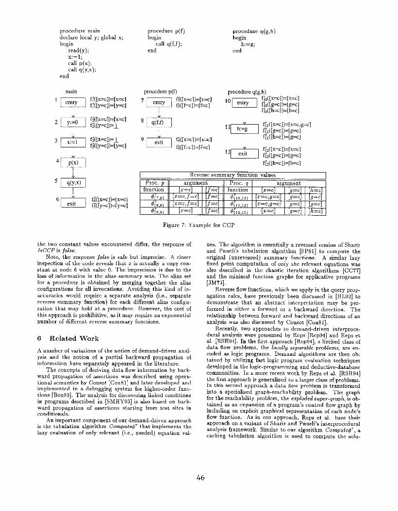
{G,,..., Gk } where Gp = (lVP, EP) is a directed flow graphrepresenting procedure p. Nodes in NP represent the state-ments in p and edges in Ep represent the transfer of con-trol among statements. Two distinguished nodes rP and ePrepresent the unique entry and exit nodes of p. The setE = u{E,ll < z < k} denotes the set of all edges in G,N = u{N, I1 < z < k} denotes the set of all nodes in G andpred(n) = {ml(rrz, n) c E,} and succ(n) = {ml(n, m) E E,}denote the set of immediate predecessors and successors ofnode n, respectively. We assume that IEl = 0( I.NI). Finally,IVc.il ~ N denotes set of nodes representing procedure ca.lk(call sites) and for each node n c NCail, call(n) denotes theprocedure called from n. An example of an IFG is shown inFigure 1.

During the analysis, only vaiid interprocedural executionpaths should be considered. An execution path rr is valid if~ returns after a procedure exit node eP to the matchingcall site that most recently occurred in r prior to eP. Fora node n in an interprocedural flow graph G, lP(r~~*~, n )denotes the set of valid execution paths from the programentry node r~a,~ to node n. For example in Figure 1, thepath 1,2,3,4,6,7,10, 11,4,5 is a valid execution path, whilethe path 1,2,3,4,6,7, 10, 11,9, 11,4,5 is not valid. Note thatinterprocedural execution paths are not directly representedin an IFG since it does not contain explicit edges betweencall and procedure entry nodes or between procedure exitnodes and return nodes.

Throughout this paper we assume that G is an interpro-cedural flow graph representing some program P.

2.1 Interprocedural Analysis Framework

Data flow problems are solved by globally gathering informa-tion from a domain set of program facts. This informationgathering process is modeled by a pair (L, F), where:

- L is a complete lattice with a partiaJ order Q, a least el-ement 1 (bottom), a greatest element T (top), and a meetoperator n (greatest lower bound) and a dual join operatorU (least upper bound). L has the decreasing chain property(i.e., any decreasing chain ZI ~ zz ~ . . . is finite). The bot-tom element L denotes “null reformation” and we assumethat the top element T denotes “undefined information” 1.

1If ~ &e~ not already contain a top element with the meaning“undefined information” , it can always be extended to include anadditional new top element,

38

procedure main

declare a,b;

begina:=l;

read(b);

call p;end

procedure pbegin

if (cond) then a:=belse b:=l;

call p;endifi

end

main 6

1

z

entry

fl(x,,xb)=(x.,xb) ‘J

2 a:zl

procedure p

R

entry

f6(x.,xb)=(x,,xb)

if (cond)fT(x,,xb)=(xa,xh)

I I / ‘---

Af~(x=,xh)=(l ,xb)

3 read(b)

f3(xa,xb)=(xa,l )

4 call(p) 228b:=l

f~(xa,xb)=(x,,l)

9 call(p)

23@(6,11)(%,xb)=if Xh=l then (1,1)

w

0(6,11)

5 else Q- ,~) flO(x.>xb)=(xb,xb)exit

1 exit

Figure 1: An IFG with the local flow functions for copy constant propagation.

F ~ {f : L ++ L} is a set of monotone functions over L~i.e, z ~ y + j(z) ~ ~(y)).

A locrd flow function fn E F is mapped to each noden E N — iV.~LI to model the local data flow effect of exe-cuting node n. A data flow analysis is called fl-distt-ibutive

if all local flow functions are n-distributive (i.e, $(z n y) =~(z) n ~(y)).

The exhaustive solution to an (interprocedural) data flowproblem is the meet- over- all- valid-pa ths solutionmop: NwL:

If the analysis is n-distributive then the mop solution canbe computed as the greatest fixed point of a system of dataflow equations [SP81]. Data flow equations are evaluated ina two-phase approach. During the first phase the data floweffect of each procedure is analyzed independent of its callingcontext. The results of this phase are procedure summary~unctions as defined in equation system 1. The summaryfunction @(.P,eP): L w L for procedure p maps data flowfacts from the entry node rP to the corresponding set of factsthat holds upon procedure exit.

Equation System 1

The actual calling context of called procedures is propagatedduring the second phase based on the summary functions.The solution to the data flow problem is defined as the great-est fixed point of equation system 2, where x(n) describesthe data flow solution on entry of node n.

For finite lattices, Sharir and Pnueli propose an iterativeworklist-driven tabulation algorithm to solve the equationsystems 1 and 2. Their algorithm requires 0( [L I x IN I) spaceto tabulate equations from 1 and 2 and the time for O(C x

Equation System 2

For each procedure p:

I(?-p) = n x(m)WW..II and c~u(m)=P

For each procedure p and node n # rP:

( fm(x(m)) if m@NCau

x(n) = n

[

if mEN=~ll,m~pred(n) #{rq,eq)(~(m))

call(m) =q

height(L) x ILI x INI) meet operations and/or applications oflocal flow functions, where C is the maximal number of callsites calling a single procedure and hetght(L) is the heightof lattice L (i.e., the length of the longest chain in L).

2.2 Example: Copy Constant Propagation

We iUustrate our approach throughout this paper using theexample of copy constant propagation (CC P). CCP is adistributive version of the (non-distributive) constant prop-agation analysis with expression evaluation [Ki173]. A vari-able is a copy constant if it is either assigned a constantvalue or it is assigned a copy of another variable that is acopy constant. Since no expressions are evrduat ed, CCP isless expensive but may dkcover fewer constants than con-stant propagation with expression evaluation. Recent stud-ies on interprocedural constant propagation [GT93] indicatethat the discovery of constants based on copies may be aseffective in practice for the interprocedural propagation asthe more costly discovery of constants based on symbolicevaluation.

A demand-driven algorithm for interprocedural copy con-stant moDa~ation limits the analvsis effort to the discoverv

constants in-

.“

of the-interesting interprocedural constants. For example inparallelization, the interesting interprocedural

39

undefinedA

. . . cl-l c, Cl+l ‘ constant

-Lany integer

Figure 2: The component lattice for copy constant propa-gation for a single program variable.

elude the values of variables or formal parameters that occurin array subscript expressions or in loop bounds.

Determining that a variable w is a copy constant requiresthe simultaneous analysis of all programs variables. CCP isnot a partttzonable [Zad84] analysis that would permit theseparate analysis of each variable as, for example, is possiblein live variable analysis. The CCP lattice for a programwith k variables is the product Lk, where the componentlattice L is defined as shown in Figure 2. Thus, each latticeelement z ● Lk is a k-tuple with one component (z)O E L

for each variable W. The meet operator n and the dual joinoperator u are defined pointwise according to the partialorder depicted in Figure 2. Of particular interest are thebase elements in Lk. A base element is a tuple x indicatingthat a single variable v has some constant value c and thatalf other variables are not constant: (z). = c and (fl)~ = 1

for w # v. We use the simplified notation [V=C]C Lk for sucha base element x. For readabifit y, we also write [w=c, W=C]for the join of base elements: [o=c] U [w=c]. Furthermore,we also use T and 1 for the top and bottom element of theproduct lattice Lk.

We define the distributive flow functions j in CCP point-wise for each component corresponding to one of k variables,i.e., .f(zl, . . ..z~)=f(zlzl ,.. .,xk)l, ..., .f(Zl,..., Zk)k). The

component .f(z I, . . . . Xk)W of a local flow function .f with re-spect to variable w is defined in Table 1 for various typesof assignments. The local flow function for a conditionalexpression is simply the identity function

locaf flow function component ~.(z) ~,node n

wherez= zl, . . ..z~

V:=c fn(z)w = ~: yt;e;’:e

fn(z)w = ;:Zfv=w

IJ:=’Uotherwise

u:=tor

read(v)fn(z)w = ,: j;e;’:e

Table 1: The local flow functions in CCP, where u, v and u]

are variables, c is a constant and t is an expression.

In Figure 1, the local flow function associated with eachnode is shown below the node. Each lattice element is a pair(t., z,), where the first and second component denote latticevalues for variables a and b, respectively. The executioneffect of procedure calls (nodes 4 and 9) is modeled by the

summary function @(G,l1, as defined in equation system 1.The full definition of $4 fj,]I) is shown only at node 4.

3 Propagating Data Flow Queries

A data flow query q raises the question as to whether aspecific set of facts y c L is a safe approximation of the

exhaustive solution at a selected program node n. A latticeelement y is a safe approximation of the solution x(n) if yis lower in the lattice than z(n).

Definition 1 (Data flow query) Let y s L and n c N.A data flow query q is of the form q =< y, n > and denotesthe truth value of the term: y L z(n).

For the program in Figure 1, consider the question asto whether variable a is a copy constant after returningfrom the calf to procedure p from rnazn, i.e., on entry ofnode 5. The least lattice element that expresses that a hassome arbitrary but fixed constant value c is the element(a=c, b= J-) = [a=c] (i.e., variable 11may assume any value).Thus, the question corresponds to the query q =<[a=c], 5>.

We now consider the problem of determining the answer(true or ~alse) for a query q without exhaustively evaluat-ing the equation systems 1 and 2. Informally, the answerto q=<y, n> is obtained by propagating q from node n inreverse direction of the original analysis until all nodes havebeen encountered that contribute to the answer for q. Wemodel thk propagation process as a parttcd reversal of theoriginal data flow analysis.

To illustrate the reversal of the analysis we examine thefollowing cases in the propagation of q =< y, n >.

Case (i) (Node n = r~a,~): no further propagation of q

is possible and q evaluates to true if and only if y = J_.Case (ii) (Node n = rP for some procedure p): q raises the

question as to whether y holds on entry of every invocationof p. It follows that q can be translated into the booleanconjunction of queries < y, m > for every call site m callingprocedure p.

Case (iii) (Node n is some arbitrary non-entry node): Forsimplicity, assume for now that n has a single predecessorm. Equation system 2 shows that y G z(n) if and onlyif y ~ h(z(m)), where h is either a local flow function ora summary functiou. By the monotonicity of h, the termy G h(z(m)) directly evaluates to true if y ~, h(l) andto false if y Q h(T). Otherwise q translates mto a newquery q’ =< z, m > for node m. The lattice element z tobe queried on entry of node m should be the least element(i.e., smallest set of facts) such that z L x(m) implies y ~h(z(m)). To find the appropriate query element z for thenew query g’ we apply the reverse function h“ [HL92].

Definition 2 (Reverse function) Given a complete lat-

tice L and a monotone function h : L ++ L, the reversefunction h’ : L ++ L is defined as:

h’(y) = n {z E L : Y E h($)}

The reverse function h’ maps y to the smallest element zsuch that y ~ h(z). Note, that if no such element exists

h“(y) = T (undefined).If the function h is n-distributive then the following rela-

tionship holds between function h and its reverse h’ [COU81,HL92]:

y ~h(z) + h’(y) ~z (GC)

The above relationship uniquely determines the reverse func-tion and defines a Galois connection [Bir84] between h andits reverse h’. Note, that the n-distributivity is necessaryfor establishing this relationship. For the remainder of thissection we consider only distributive flow function and showhow the resulting relationship between flow functions and

40

their reverse functions can be exploited during the querypropagation.

First consider the following properties of the functionreversal. It can easily be shown that the fl-distributivityof h implies the I-1-distributivity of the reverse function h’:/Z’(ZUy) =lZr(X)LIh’(y). Lemma lstates relevant propertieswith respect to the composition, the meet and the join offunctions.

Lemma 1 Let g and h be two fl-distributive functions.

(i) (g. h)’ = h’ ~g’

(ii) (gmh)’ = g’ uh’

Proof: straightforward and omitted for brevity (see also[HL9z]).

Table 2 shows the definition of the reverse flow functionsin CCP. For all flow functions ~~ (T) = T and ~~(1-) =1. By the LI-distributivit y of the reverse functions, it is~u$icient to define ~~ for the base elements in the latticeL.

node n reverse flow function f; ( [w=c] )ifw=v, C=c’

U:=CJ if w=v, c#c’

[w=cl otherwise

?J:=Uif w =V

.fl([w=cl){ {~~j] o~herwise

v:+, if w =Vf;([w=c]) [WLC] otherwiseread(v)

Table 2: The reverse local flow functions in CCP.

The reverse function value f: (~w=cl) denotes the least lat---- ..tice element, if any exists, that mus~ hold on entry of noden in order for variable w to have the constant value c onexit of n. If f~([v=c]) = J-, the trivial value 1 is sufficienton entry of node n (i.e., v always has value c on exit). Thevalue f: ([v=c]) = T indicates that there exists no entryvalue which would cause v to have the value c on exit.

The following propagation rules result immediately fromthe definition of the exhaustive equation system 2 in a n-

distributive data flow framework and the properties of thereverse functions. The operator A denotes the boolean ANDoperator.

Query Propagation (distributive functions)

{

true< y, r~.$. > U

ify=l

false otherwise

<y, rP> *A

<y)m>

nzeNc.ll, call(m)=p

fake if hmr(y)=T

<y, n>u

‘{

true if h~’(y)=l.

771Gpred(n) < h~’ (y), m > otherwise

{

f?n if m $ Ncauwhere h~ =

q$(rp,ep) if m 6 N.~U, call(m) = p

The propagation rules require the application of reversefunctions. If node m is not a call site the reverse function

f; can be determined by locally inspecting the (distributive)flow function ~~. Otherwise, if node m calls a procedure pwe need to determine the reverse summary function 4[TP,.P).

We first assume in the next section that all necessary reversesummary functions are available and then discuss their de-termination in detail in the following section.

3.1 Query Algorithm

The demand algorithm Query that implements the querypropagation rules is shown in Figure 3. Query takes as in-put a query q and returns the answer for q after a finitenumber of applications of the propagation rules. Query usesa worklist initialized with the input query q. The answerto q is equivalent to the boolean conjunction of the answersto the queries currently in the worklist. During each step aquery is removed from the worklist and translated accordingto the appropriate propagation rule associated with the nodeunder inspection. The query resulting from this translationis merged with the previous query at the node and addedto the worklist unless the previous query haa not changed(lines 7-8 and 15-16). The algorithm terminates with theanswer true if the worklist is exhausted and all queries haveevaluated to true. Otherwise, false is returned.

Query(y, n)

1. for each m ~ N do query [m] + -1-2. cpter~[n] + y; worklisi+ {n};3. while wo.klist # 0 do4. remove a node m from worklisfi5. case m = Tq for some procedure q:6. for each m’ ~ Nca[l s.t. call(rn’) = q do7. query[m’] + que~~[m’] U qtiery[m];

8. if query[m’] changed then add ml to workks~

9. endfor;10. otherwise:11. for each m’ c p~ed(m) do

{

f~, (werv[ml) if m’ @NCall

12. new +‘?_r,,eg)

(query[m]) if m’cNcall,

call(m’)=u

13. if (new ~ T) then return( false )‘ ‘ “

14. else if (new 3 1) then15. query[m’] + query[m’] U new;

16. if queTy[m’] changed then add m’ to worklis~

17. endif;18. endfor;

19. endwhile;20. return(true);

Figure 3: Generic demand algorithm Query. Query(y, n)returns the response true or false to the query q =< y, n >.

To determine the complexity of the query algorithm wecount the number of times a join operation or a reversefunction application is performed. A join/reverse functionapplication is performed at a node n in lines 7, 12 and 15only if the query at a successor of n was changed (or at theentry node of a procedure p if n is a call site of p) which canhappen only O(height(L)) times. Hence, algorithm Queryrequires in the worst case O(height(L) x INI) join operationsand/or reverse function applications.

If the program under analysis consists of only a singleprocedure (the intraprocedural case), Query provides a com-plete procedure for demand-driven data flow analysis. Forthe inter-procedural case, we require an efficient procedure tocompute the reverse summary functions, as discussed next.

41

Comptitecjr(p, y)1. if M[eP, y] = y then /8 result pr-e.aously computed */

2. return (M[rP, y]);3 wodi-W+{(ep,y)}; M[ep,Y]=Y;

4. while woTkiist #@do5. remove a pair (n, z) from worklist and let z + M[n, r];

6. case neNCall and call(n) =q:

7. if M[eq, 2] = 2 then8. for each m c p.cd(n) do9. Propagate(m, x, M[~~, z]);

10. else /* tTiggeT computation of 4~rq,eq~(~) */

11. M[eq, z] + z and add (eq, z) to woTklisti12. case n = rq for some proc. q:

/* Pvopagate z to call sites if needed */

13. for each m E N=all such thatcall(m) = q and M[m, z’] = z for some z’ do

14. for each m’ c pred(m) do Propagate(m’, z’, z);

15. otherwise:/*nisnot acallsite andnotan entry node */

16. for each m C pTed(n) do %-wag~tc(m, Z, jl(z));

17. endwhile;18. return(M[rP, y]);

Propagate(n, y, new) /* propagate new to M[n, y] */

1. M[n, y] + kf[n,y] u new;2. if M[n, y] changed then add (n, g) to worklis~ endi~

Figure 4: Compute#r(p, y) returns the reverse summaryfunction value ~~r, ,ep)(y) for a procedure p and y 6 L.

3.2 Reverse Summary Functions

This section discusses an algorithm to compute individ-ual reverse summary function values in order to extend al-gorithm Query to the interprocedural case. An obvious andinefficient way to compute reverse summary functions is tofirst determine all origim-d summary functions by evaluatingequation system 1 and then reverse each function. We de-scribe in this section a more efficient method to directly com-pute the reverse functions. Our algorithm mirrors the oper-ations performed in Sharir and Pnueli’s worldist algorithmfor evaluating equation system 1, except that we computereverse summary function values and the direction in whichtable entries are computed is reversed. Assuming that theasymptotic cost of meet and local flow function applicationis the same for join and reverse flow function application,our akorithm has the same worst case comdexitv as Sharir

“ .“

and Pnueli’s algorithm for the original summary functions.As in Sharir and Pnueli’s algorithm the tabulation strategyrequires the lattice L to be finite.

We first derive an inductive definition of the reverse sum-mary functions from equation system 1. By reversing theorder in which summary function are constructed and byapplying Lemma 1 we obtain the following definition of thereverse summary function #~,p,eP) for each procedure P:

Equation System 3

Figure 4 shows an iterative work!ist algorithm Compute~r

that, if invoked with a pair (p, u), returns the value ~f., ,.P ) (Y)

after a partial evaluation of the equation system 3. Individ-ual function values are stored in a table M : N x L + L such

that ~[n, g] = 4{n,eP)(y). The table is initialized with 1 andits contents are assumed to persist between subsequent callsto procedure Compute@r. Thus, results of previous calls arereused and the table is incrementally computed during a se-quence of calls. After calling Computexj’ with a pair (p, y)a worldist is initialized with the pair (eP, y). The contentsof the worklist indicate the table entries whose values havechanged but the new values have not yet been propagated.During each step a pair is removed from the worklist, itsnew value is determined and all other entries whose valuesmight have changed as a result are added to the worklist.

We next analyze the cost of k calls to Computeq5r. Stor-ing the table A4 requires space for [N\ x [LI lattice elements.To analyze the time complexity we count the number ofjoin operations (in procedure Propagate) and reverse flowfunction applications (at the call to Propagate in line 16).The loop in lines 4-17 is executed O(hezght(L) x ILI x INI)times, which is the maximal number of times the latticevalue of a table entry can be raised, i.e., the maximal num-ber of additions to the worklist. In the worst case, the cur-rently inspected node n is a procedure entry node. Pro-cessing a procedure entry node r~ results in calls to Prop-

agate for each predecessor of a call site of procedure q.Thus, the k calls to Compute@’ require in the worst caseO(C x height(L) x ILI x INI) join and/or reverse functionapplications, where C is the maximal number of call sitescalling a single procedure.

Assuming that each access to a reverse summary func-tion in procedure Query is replaced by an appropriate callto Compute@’, the total cost of algorithm Query is O(C xheight(L) x l~\ x IN[) join and reverse local flow functionapplications plus the space to store 0( INI x ILI) lattice ele-ments.

3.3 Queries in non-distributive Frameworks

The distributivity of the original analysis framework is nec-essary to ensure that queries are decidable, that is, to ensurethat the query propagation rules from the previous sectionyield as precise information as the original exhaustive analy-sis does. We consider in this section the kind of approxima-tion that is obtainable if the query propagation rules are ap-plied to evaluate queries in the preseuce of non-distributiveflow functions.

If all flow functions in a data flow framework are i’l-distributive then a data flow query < y, n > evaluates totrue if and only if element y is part of the solution at noden, i.e., if and only if y c x [n]. If the original analysis frame-work is monotone but not n-distributive then informationmay be lost during the query propagating process. Specifi-cally, if a flow function h is monotone but not distributive,then the relation between h and its reverse h‘ is weakerthan in the distributive case; only the following implicationholds (see in contrast the Galois connection (GC)):

y ~ h(z) =+ h’(y) gz

As a result of this weaker relationship queries are only semi-decidable in the presence of non-distributive flow functions.Conceptually, the derived query algorithm may also be ap-plied to data flow problems with non-distributive functions.In the presence of non-distributivity, the above implicationensures that if a query q =< y, n > evaluates to false theny ~ x [n]. However, nothing can be said if q evaluates totrue. If appropriate e worst assumptions are made for true

42

responses, the query algorithm still provides approximate

information in the presence of non-distributive flow func-

tions.

4 Optimized Query Evaluation

This section discusses two ways to improve the performanceof the query evaluation. The choice of optimization dependson whether a fast response to (i) a single query or to (ii) asequence of queries is of primary int crest.

To optimize the response time for a single query, thequery evaluation includes earlg termination. Recall that the

answer to the input query is the boolean conjunction of the

answers to the queries currently in the worklist. Thus, the

evaluation can directly terminate as soon as one query eval-

uates to fcd.se, independent of the remaining contents of the

worklist. Early termination is included in algorithm Query

in Figure 3.

To process a sequence of k queries requires k invocations

of Querg, which may result in the repeated evaluation of the

same intermediate queries. Repeated query evaluation can

be avoided by maintaining a result cache. We outline a sim-

ple extension of algorithm Query to include result caching.

A global cache is maintained that contains for each node

n and lattice element y an entry cache [n, g] denoting theprevious result, if any, of evaluating the query < g, n >.Before a newly generated query q is added to the worklist,the cache is first consulted. The query q is added to theworklist only if the answer for q is not found in the cache.Entries are added to the cache after each terminated queryevaluation. Recall that a false answer at some node n im-plies a false answer for all previously generated queries atnodes that are reachable from n along some valid executionpath. Thus, the cache can be updated in a single pass overthe nodes that have been visited during the current invoca-tion of Query. First, each visited node n that is reachablefrom a node that evaluated to false is processed and thecache is updated to cache[n, guerg[n]] = false. Note, thatat this point the entries cache[n, z] for query [n] L z couldalso be set to false. For the remaining visited nodes n, where< query[n], n > evaluated to true, the cache is updated tocache[n, querg[n]] = true. Again, the entries cache[n, z] forz L guerg[n] could also be set to true.

The inclusion of result caching has the effect of incre-mentally building the complete (exhaustive) data flow so-lution during a sequence of calls to Quer-g. Result cachingdoes not increase the asymptotic time or space complexityof algorithm Querg. Storing the cache requires O(INI x ILI)space and updating the cache requires less than doublingthe amount of work performed during the query evaluation.Moreover, the asymptotic worst case complexity of k invo-cations of Querg with result caching is the same for anynumber k, where 1 ~ k ~ ILI x INI and ILI x INI is thenumber of distinct queries.

5 Copy Constant Propagation

This section illustrates our approach for the problem of in-terprocedural copy constant propagation. Using this exam-ple we show how the query algorithm can be extended tohandle programs with formal reference parameters and lo-cal variables. The difficulty introduced with formal referenceparameters is the potential of aliasing. Ignoring aliasing

refined 1ocal flow function ~n(z),node n

wherex= zI, . . ..z~)

{

c i.fw=v

V:=c fn(x)w =XW n c if wcalias(v, n),

w#v

Xw otherwise

{

Xu ifw=v

V:=u fn(x)w =xwnxu if w~alias(v, n),

w#vx,,, otherwise

1 if w C alias(v, n)red(v)> fn(x)w = ~wV:=t otherwise

Table 3: Local flow functions in CCP refined based on may-alias information.

~de n refined reverse local flow function f;

(1. ifw=v

{

‘ f;([w=c]) = T

and c = C’:=C zf wcaiias(v, n)

and c # c’

[w=c] otherwise

{

[ZL=c] ifw=v

f;~~w=cl~ = [w=c, u=c] ~ ;~lias(v, n),:=U

[VJ=c] otherwise

T if wcaiias(v, n)ad(v), i:([w=c]) = [W=c] otherwise_—t

Table 4: Reverse local flow functions in CCP refined basedon may-alias information.

during the analysis may lead to unsafe (i.e., invalid) queryresponses. We show how alias information can be incorpo-rated to ensure safe answers to queries.

For simplicity, we assume programs with flat scoping.The address space Addr(p) of a procedure p is defined as:Addr(p) = Global U Local(p) U Formal(p), where Global is

the set of global variables in the program, Local(p) is theset of variables local to p and Formal(p) is the set of formalparameters of p.

Two variables z and g are aliases in a procedure p if xand g may refer to the same location during some invocationof p. Reference parameters may introduce aliases throughthe binding mechanism between actual and formal parame-ters. The determination of precise ahas information is NP-complete [M ye81]. Therefore, we assume that approximate ealias information is provided for each procedure p in form ofa summary relation alias(p) as described in [CO085]. A pair(z, y) c alias(p) if z is aliased to gin some invocation of p

(ma@iases). We use alias(z, p) = {g I (x, g) G alias(p)}

to denote the set of mug aliases of x in p and alias(x, n) =

aiias(z, p) if node n is contained in p.

The computation of the aiias(p) sets can be expressedas a distributive data flow problem with a finite domain setover a program’s call graph [CO085]. Thus, we can employthe demand-driven analysis concepts from the previous sec-tion in order to compute only the relevant alias pairs inprocedures that are actually analyzed. However, to avoidconfusion in discussing the refinements in this section wemake no assumption on how the alias information is com-puted but assume that sets aiias(p) are available to the CCP

43

algorithm for each procedure p. Using these alias sets we re-fine the local flow functions from Section 2 to safely accountfor the potential of aliasing. More precise refinements arepossible if, in addition to may alias information, must aliasinformation is available. The refined local flow functions andthe corresponding refined reverse flow function are shown inTable 3 and Table 4, respectively.

The equation system 3 for the determination of reversesummary functions is refined to express the name bindingmechanisms of reference parameters at call sites. We de-fine a binding function bs for each call site s that maps alattice element x from the calling procedure to the corre-sponding element bs(z ) in the called procedure according tothe parameter passing at s. We will also need to considerthe reverse binding b~l to translate a lattice element from acalled procedure to the corresponding element in the callingprocedure. Let s be a call site in a procedure p that passesthe actual parameters (up], . . . apj ) to the formal parame-ters (fpI, . . . fpj ) in the called procedure q. Furthermore,let w c Addr(p) and w ~ Addr(q):

where U = ({w} n Global) U {fp, I apt = v}

{

[W=c] if WE Global

b;’ ([w=c]) = [ap,=c] if w=fp,

1 otherwise

The functions b. and b~l are U-distributive and bs (T) =b:l(T) = T.

Equation system 4 shows the refined definition of reversesummary functions. The equations in 4 are defined for baseelements ~o=cl, where v c Addr(p). If v @ Addr(p) then

~tr,,ep)([i=c]j= [V=c].

Equation System 4

‘te.,e,)([u=cl) = [V=c] for each procedure p

( .f~ d{m,ep)([w=cl)

( ifrnCiVcat,, call(m)= q

Finally, we refine the query propagation rules using the biud-ing functions. The refinement is shown for queries with re-spect to the base elements in a procedure p, wheren ~ NP-Ncall and uc Addr(p). For an arbitrary set of base

elements B, the query < ~~~ b, n > is equivalent to the con-

junctionA

<bjn>

beB

Refined query propagation in CCP

< [v=cJ, rp > * ~ < [b;’(v) =c],m >

mEN..,, ,Cdl(m)=p

< [v=c], n > U

false if f~([v=cl) =T

‘1

true if ~L([v=cl)=J-

rn c precl(n), < $;([v=c]), m > otherwise

m E N.. Iz

false if h~([v=c])=T

A

‘1

true if hm([v=c])=l

m ~ pred(n), < hm([v=c]), m > otherwise

m c iV.. zz,can(m) = p

5.1 CCP Query Algorithm

Figure 5 shows algorithm IsCCP to respond to a query ofthe form “Is variable v a copy constant at node n?”. If vis a copy constant at n then Is CCP returns the constantvalue c of v. Otherwise IsCCP returns false. Note, thatthis query format is more general than previously discussed.More specific queries of the form “Is v a copy constant at nwith value c?” can always be answered using the responseof Is CCP.

Algorithm 1sCCP is an inst ante of the generic algorithmQuery from Section 3, except that IsCCP also includes therefinements for reference parameters. To handle the moregeneral query format, the specification of a constant value cis simply dropped; a base element [v=c] simplifies to [v] anda query < [v], n > raises the question as to whether variablev has some arbitrary but fixed constant value at node n. Aquery < [v], n > evaluates to true at a node n if node nassigns any constant c to variable v, in which case the valuec is remembered. If all generated queries evaluate to true

the join over the remembered constant values is examined.If this join yields a constant c, then c is returned. Otherwisethe response is false.

The corresponding instance of the generic procedureComputeq$’ , shown in Figure 6, partially evaluates the equa-tion system 4. By the distributivity of the reverse summaryfunctions, it is sufficient to maintain table entries only forbase elements resulting in MaxAddrx N entries, where Max-

Addr is the size of the maximal address space in any pro-cedure. Each entry may contain a set of base elements andis therefore of size MaxAddr. To keep track of the actualconstant values encountered, the table M includes an extrafield Mb, v]. val for each procedure p and each variable v.

We now consider the cost of procedures IsCCP andComputeq$’ not including the cost of computing the alias in-formation. During an invocation of IsCCP a total of0( I!4axAcMr x INI) queries may be generated resulting in0( MaxAddr x IN [) join and reverse function applicationsin procedure IsCCP. The fixed point computation of tableentries in procedure Compute#r requires in the worst case0( MazAddr2 x INI) table entry updates. As in the generalcase, each table update may trigger up to C join and/orreverse function applications, where C is the maximal num-ber of call sites calling a single procedure. Assuming joinand reverse function applications are performed pointwise,each join or function application requires 0( M ax Addr ) timeresulting in the total time of O(C x MaxAddr3 x IN l).

44

IsccP(?J, n)

1. for each m 6 N do guery[m] + O;

2. query [n] + [v] ; worklist 4- {n}; val = 1;3. while worklist # 0 do4. remove a node m from worklist;

5. let p be such that m c Np;

6. case m = r~ for some proc. q:

7. for each m’ c NcaLt s.t. call(m’) = q do8. quepy[m’] + query[m’] U b~l (query [m]);

9. if qaery[m’] changed then add m’ to worklis~

10. endfor;11. otherwise:

12. for each m’ c pred(m) do

{

.f~, (~uery[ml) if m’#NCall

13. new i- b~~ (Compufeq$r(q, bm, (z), val), if m’~NCall,where x = alias(query[m], p) catl(m’)=g

14. if new = L and m’ ~ NC.ll then vat + val U c,where c is the constant assigned at m’;

15. if new = T or val = T then return( false )16. else if new 2 1 then17. /* query still unresolved */

18. que~y[m’] + query[m’] U new;19. if qtie~y[m’] changed then add m’ to worklist;

20. endifi

21. endfor;

22. endwhile;

23. if val < T then return(val) else return(.fake);

Figure 5: Demand algorithm for CCP. IsCCP(V, n) returnsthe constant c if variable v is a copy constant at node n withvalue c, otherwise it returns false.

5.2 CCP Example

We illustrate algorithm 1s(7CP for copy constant propaga-tion using the program example in Figure 7. The pro-gram consists of three procedures main, p and q, whereGlobal = {z}, Local(main) = {y}, Formal(p) = {f} andFormal(q) = {g, h}. The may-alias relations are: alias(p) ={(z, f)} and aiia~(q) = {(z, h), (X,9), (v, g), (g, h)}. The re-verse local flow functions are shown next to each node inthe IFG. The table in Figure 7 shows the reverse summaryfunctions. In addition to the reverse summary function en-tries for the base elements in each procedure (rows for 4~7,9)

and q$(lO,l,)) the table also shows intermediate entries (last

two rows) collected during the computation of the summaryfunctions. We consider the evaluation of the following queryexamples:

Query 1: ?lsCC’P(h, 10) ( “Is the formal h of procedure q

a copy constant on entry of each invocation of q“ ?):

Initially, worldist = {10} and query[lO] = [h]. Qtiery[lO] ispropagated to queries for the corresponding actual parame-ters at call sites resulting in: query [5] = [z] and qaery[8] =

[f]. processing quev[8] causes the propagation of [f] tonode 7 and in turn to actual parameters at the call site atnode 4, i.e., query [4] = [z]. Assume guery[5] is processednext. The global z is passed to formal ~ of procedure p at

node 4. Therefore, the reverse summary function 9$(7,9)isinspected for the two arguments [z=c] and [f =c]. The newquery element resulting for node 4 is determined as query [4]= ~11(4;7,9) ([~=d) u 4;7,9)([f=cl)) = r ([$=clf=cl) =

[z=c], which is simplified to [z]. Applying the reverse func-tion yields fl”([z]) = J-, i.e., the query at node 4 evaluatesto true and 1 is remembered as the actual constant assigned.

Compute~r(p, y, val)

1. worklist + 0; res + 1;

2. let y = [VI, . . . . V~], where v, 6 AddT(p);

3. for each v;, where 1 ~ i ~ k do

4. if M[eP, v,] = 1 then add (ep, v,) to woTklis~

5. M[ep, v,] = [w]; endif;6. while worklist # @ do

7.

8.9.

10.11.

12.

13.14.

15.

16.17.18.

19.20.

21.22.23.

24.25.

26.

27.28.

29.

30.31.32.

33.34.

35.36.

37.

remove a pair (n, w) from worklisfi

let p’ be the proc. containing n;let [wI, . . ..wj] = M[n, w];

case n E Ncall and call(n) = q:

for each w,, where 1< i ~ j do

if w% c Global or w$–isan actual param. at n thenfor each z 6 bn([w,]) do

if M[e~, z] = [z] then

for each m c pred(n) do

P~opagate(m, w, b~l(M[rq, z]));

if M[rq, z] = 1 thenM~’, w].val + M[p’, w].val U M[q, z].val;

else M[eq, Z] + [z]; add (eq, z) to worklist; endifiendfor;

else /* skip call site if u not passed */

for each m G pred(n) do Propagate (m, w, [w,]);endfor;

case n = ~q for some procedure g:for each m c Ncall such that

call(m) = q and b~l([w]) c M[m, z] for some z do

/* i.f entry M[r~, w] was .eq’aested earlier */let p“ be the proc. containing m;for each m’ G pred(m) do

Propagate(m’, z, b~l (M[n, w]);

if M[rq, w] = L then

M[p”, z].val i- &f[p”, z].val U &f[q, w].vai;otherwise:

for each m c pred(n) doPropagate(m, w, .f&(M[n, w]);

if ~~(M[n, w]) = L then&f[p’, w].val + M[p’, w].val U c, where

c is the const. assigned at m;

38. endwhile;39. for each v,, where 1 ~ i ~ k do40. res e res u M[rp, vt]; val e val u hf[p,v~].val; endfor;41. return(res);

Propagate(n, v, new) /* propagate new to M[n, v] ‘/1. M[n, v] + M[n, v] U new;

2. if M[n, v] changed then add (n, v) to worklis~ endifi

Figure 6: Algorithm Compute@” (p, y, vai) in CCP returningthe value +;,, ,eP)(v) for a procedure p and y ● L.

Since the worhlist is exhausted, the overall response is 1,indicating that the formal h of procedure q always has thevalue 1 on entry of procedure q.

Query 2: ?Isc7CP(Z, 6) ( “Is variable z a copy constantafter the call to procedure q at node 6“ ?):Initially, worldist = {6} and quepg[6] = [x]. Processingque~y[61 results in: query[5] = b~’ (@~10,12)([I=C] U [h=c]))

= b~l ([z=c,g=c]) = [z=c,v=c] which is simplified to [x, y].We consider the propagation of the query elements [z] and[y] separately. Since y is local to main, [y] directly prop-agates through nodes 4 and 3. At node 2: ~~([y]) = 1and the value O is remembered as the actual constant as-signed. As for Query 1, propagating the query element [z]from query [5] will eventually lead to the evaluation true atnode 4 with 1 being the actual constant assigned. Since

45

procedure main

declare local y; global x;

begin

read(y);X:=1;

call p(x);

call q(y,x);

end

main

1

T

ff([x=c])=[x=c]entry

ff([y=c])=[y=c]

2

$

f;([x=c])=[x=c]y:=of;([y=c])=~

3 X:=l f;([x=c])=~f;([y=c])=[y=c]

v--%---5

2

CI(YJ)

6 f:([x=c])=[x=c]exit f+([y=c])=[y=c]

procedure p(f)

begin

call q(f,f);

end

procedure q(g,h)

begin

h:=g;

end

procedure p(f) procedure q(g,h)

7 Ff;([x=c])=[x=c]

entryf+([f=c])=[f=c]

7

10 entry

8

2

q(f,f) 111 h:=g

9 exit f;([x=c])=[x=c]

f;([f=c])=[f=c] 1,121 exit

fi~([X=C])=[X=C]ffo([g=c])=[g=c]fio([h=c])=[h=c]

fil([X=C])GIXcC, g=C]fi~([gEC])D[gDC]fil([hmc])=[g=c]

fi~([XmC])c[XEC]fi*([gGC])z[gGC]

fil([h=c])c[h=c]

Reverse summary function values

Figure7: Example for CCP

the two constant values encountered differ, the response of

IsCCP is fake.

Note, the response @seis safe but imprecise. A closer

inspection of the code reveals that z is actually a copy con-

stant at node 6 with value O. The imprecision is due to the

loss of information in the alias summary sets. The alias set

for a procedure is obtained by merging together the alias

configurations for all invocations. Avoiding this kind of in-

accuracies would require a separate analysis (i. e., separate

reverse summary function) for each different alias configu-

ration that may hold at a procedure. However, the cost of

this approach is prohibitive, asitmay require an exponential

number of different reverse summary functions.

6 Related Work

A number of variations of the notion of demand-driven anal-ysis and the notion of a partial backward propagation ofinformation have separately appeared in the literature.

The concepts of deriving data flow information by back-ward propagation of assertions was described using opera-tional semantics by Cousot [COU81] and later developed andimplemented in a debugging system for higher-order func-tions [Bou93]. The analysis for discovering linked conditionsin programs described in [SMHY93] is also based on back-ward propagation of assertions starting from test sites inconditionals.

An important component of our demand-driven approachis the tabulation algorithm Comp uteq$’ that implements the

lazy evaluation of only relevant (i.e., needed) equation val-

ues. The algorithm is essentially a reversed version of Sharirand Pnueli’s tabulation algorithm [SP81] to compute theoriginal (unreversed) summary functions. A similar lazyfixed point computation of only the relevant equations wasalso described in the chaotic iteration algorithms [CC77]and the minimal function graphs for applicative programs[JM731.

Re~erse flow functions, which we apply in the query prop-agation rules, have previously been discussed in [HL92] todemonstrate that an abstract interpretation may be per-formed in either a forward or a backward direction. Therelationship between forward and backward directions of ananalysis was also discussed by Cousot [COU81].

Recently, two approaches to demand-driven interproce-dural analysis were presented by Reps [Rep94] and Reps etal. [RSH94], In the first approach [Rep94], a limited class ofdata flow problems, the locally separable problems, are en-

coded as logic programs. Demand algorithms are then ob-tained by utilizing fast logic program evaluation techniquesdeveloped in the logic-programming and deductive-databasecommunities. In a more recent work by Reps et al. [RSH94]the first approach is generalized to a larger class of problems.In this second approach a data flow problem is transformedinto a specialized graph-reachability problem. The graphfor the reachability problem, the exploded super-graph, is ob-

tained as an expansion of a program’s control flow graph byincluding an explicit graphical representation of each node’sflow function. As in our approach, Reps et al. base theirapproach on a variant of Sharir and Pnueli’s interproceduralanalysis framework. Similar to our algorithm Compute@’, acaching tabulation algorithm is used to compute the solu-

46

tion over the graph that. However, the graph-reachabilityalgorithm imposes more restrictions on the problems thatcan be handled than our approach. Specifically, the graph-reachability approach is applicable to problems where thelattice is apowerset over a finite domain set and where allflow functions are distributive. Although we require distri-butive functions to ensure precise data flow solutions, ouralgorithms still provide approximate information in the pres-ence of non-distributive functions. Our approach is less re-strictive on the lattice structure in that it is applicable to

any finite lattice. The restriction to a finite lattice doesnot even apply if our approach is used for z’ntraproceduralanalysis.

The utility of demand-driven analysis algorithm has alsobeen demonstrated in a number of demand-driven algorithmsdeveloped for specific analysis problems, including the fol-lowing problems. Babich et al. [BJ78] presented a demandalgorithm for intmprocedural live variable analysis based on

attribute grammars. Strom and Yellin [SY93] presented ademand based analysis for typestate checking. The authorsexperiment ally demonstrate that their goal-oriented (anddemand-driven) backward analysis is more efficient than theoriginal forward analysis for typestate checking that eagerlycollects all available information that may or may not be of

relevance. Question propagation, a phase in the algorithmfor global value numbering [RWZ88] performs a demand-based backward search in order to locate redundant expres-sions. This backward search, like our query aJgorit hm, per-forms the analysis from the points of interest (i.e., the pointswhere an expression is suspected to be redundant) and it

also uses early termination to end the search. In procedurecloning [CHK92], procedure clones are created during theanalysis on demand whenever it is found that an additionalclone will lead to more accurate information. Cytron andGershbein [CG93] described an algorithm for the incremen-tal incorporation of alias information into SSA form. Theactual optimization problem to be performed on the SSAform triggers the expansion of the SSA form to include onlythe necessary alias-information. Similar ideas have also beenimplemented in the demand-based expansion algorithm offactored def-def chains [CCF92].

Other related work addresses the goal of reducing thecost of data flow analysis by avoiding the computation ofirrelevant intermediate results. Several sparse analysis tech-niques have been presented to reduce the number of dataflow equations by either manipulating the underlying graph-ical program represent ation, such as the analyses based on

the global value graph [RT82], static single assignment form[RWZ88, WZ85], the sparse evaluation graph [CCF90], thedependence graph [JP93] or by direct manipulation of theequation system through partitioning algorithms [D GS94].Slotwise analysis [DRZ92] also falls into this class of sparsetechnique but is limited to bitvector data flow problems.Sparse analysis approaches to reduce the amount of dataflow evaluations are complementary to our demand-drivenanalysis algorithms in that the evaluation of dat a flow equa-tions is avoided independent of the specific information de-manded; that is, the evaluation of those equations is avoidedthat are irrelevant with respect to even the exhaustive so-lutions. An interesting combination of the two approacheswould be to use, for example, a reduced equation systemaccording to [DGS94] or a sparse evaluation graph as in[CCF90], as the basis for propagating data flow queries.

Incremental data flow analysis [Ros81, Zad84, RP88, PS89]has also addressed the avoidance of exhaustive solution re-

computations. However, unlike demand-driven analysis, in-cremental analysis assumes that an exhaustive solution haspreviously been computed and is concerned with avoidingexhaustive r-e-computations in response to program changes.

7 Conclusions

This paper described a new demand-driven approach to in-terprocedural data flow analysis that avoids the costly com-putation of exhaustive data flow solutions. A general frame-work for the derivation of demand algorithms covering theclass of interprocedural data flow problems with a finitedomain set was presented. In a data flow problem withdistributive flow functions, the derived algorithms provideas precise information as the corresponding exhaustive al-gorithm. In the presence of non-distributive flow functions,the derived algorithms still provide approximate solutions.We are currently exploring the utility of approximate queryresponses for non-distributive problems in practice. Par-ticularly efficient demand algorithms result for the classicalbitvector problems. For example in live variable analysis,queries about individual variables are resolved in linear timeand space if the analysis is intraprocedural or if the analysisis interprocedural and the programs are alias-free.

The goal of demand-driven program analysis is the re-duction of both the time and space cost of solving data flowproblems. When discussing result caching we implicitly as-sumed that reducing the analysis time is of primary inter-est. However, as programs grow larger, space may becomeas valuable a resource as analysis time, in particular, if re-sults for a large number of different data flow problems areto be collected. Clearly, result caching should be avoided ifthe space consumption is the primary concern. Since resultcaching is optional in our query algorithm, it can be adjustedeasily to the needs of the current application. The optionof result caching permits the computation of the completesolution with an asymptotic worst case complexity that isno worse than the cost of a standard exhaustive algorithm.To fully evaluate the benefits of the achievable time andspace reductions we are currently developing a prototypeimplementation of a demand-based query algorithm for in-terprocedural copy constant propagation.

Acknowledgements

We thank Tom Reps and the referees for their comments onan earlier draft of this paper.

References

[Bir84]

[BJ78]

[Bcm93]

[CC77]

G. Birkhoff. Lattice theory, volume 25. Ameri-can Mathematical Society, Colloquimn Publication,

Washington, DC, 3rd edition, ’84.

W .A. Babich and M. Jazayeri. The method of at-tributes for data flow analysis: Part II . Demand anal-

ysis. Acts Informuiica, 10(3), Oct. ’78.

F. Bourdoncle. Abstract debugging of high-orderimperative languages. In SIGPLAN ’93 Con.f. onProgramming Language Design and Implementation,

pages 36-45, Albuquerque, NM, Jun. ’93.

P. Cousot and R. Cousot. Static determination ofdynamic properties of recursive procedures. In E.J.

Neuhold, editor, IFIP Conj. on Formal Description

of P~ogramwzing Concepts, pa~es 237–277. North-

Hollan Pub. Co., ’77.

47

[CCF90]

[CCF92]

[CG93]

[CHK92]

[CK88]

[CO085]

[COU81]

[DGS94]

[DRZ92]

[GT93]

[HL92]

[JM73]

[JM82]

[JP93]

[Ki173]

[KS92]

J.D. Choi, R.K. Cytron, and J. Ferrante. Automaticconstruction of sparse data flow evaluation graphs.In 18th ACM Symp. on Principles of ProgrammingLanguages, pages 55–66, Orlando, FL, Jan. ’90.

J.D. Choi, R. Cytron, and J. Ferrante. On the efficientengineering of ambitious program analysis. IEEE

Trans. on Soflware Engineering, 20(2) :105-114, Feb.’92.

R. Cytron and R. Gershbein. Efficient accommoda-tion of may-alias information in SSA form. In SIG-

PLAN ’93 Conj. on Programming Language Deszgn

and Implementation, pages 36–45, Albuquerque, NM,

Jnn. ’93.

K. Cooper, M. Hall, and K. Kennedy. Procedurecloning. in IEEE 1992 Int. C’on.f. on Compute T Lan-

guages, pages 96–105, San Francisco, CA, April 1992.

K. Cooper and K. Kennedy. Interprocedural side-

effect analysis in linear time. SIGPLA N ’88 Symp. on

Compiler Constmcttonj published in SIGPLAN No-

tices, 23(7):57–66, Jun. ’88.

K. Cooper. Analyzing aliases of reference formal pa-

rameters. In 12th ACM Symp. on Principles o.f PTo-

gvamming Languages, pages 281–290, ’85.

P. Cousot. Semantic foundations of program analy-

sis. In S. MucJmick and N.D. Jones, editors, Prog~am

Flow Analysis: Theory and Applications, pages 303–342. Prentice-Hall, ’81.

E. Duesterwald, R. Gupta, and M.L. Soffa. Reducingthe cost of data flow analysis by congruence parti-

tioning. In 5th Int. Cont. on CompileT Construction,

pages 357–373, Edinburgh, U. K., Apr. ’94. SpringerVerlag, LNCS 786.

D.M. Dhamdhere, B.K. Rosen, and F.K. Zadeck. How

to analyze large programs efficiently and informa-

tively. In SIGPLAN ’92 Conj. on Programming Lan-

guage Design and Implementation, pages 212–223,San Francisco, CA, Jun. ’92.

D. Grove and L. Torczon. fnterprocednral constantpropagation: a study of jump function implementa-tions. In SIGPLAN ’93 Con.f. on Programming Lan-

guage Design and Implementation, pages 90–99, Al-buquerque, NM, Jun. ’93.

J. Hughes and J. Launchbm-y. Reversing abstractinterpretations. In ~th European Symp. on Pro-

gramming, pages 269–286, Rennes, France, Feb. ’92.Springer Verlag, LNCS 582.

N.D. Jones and A. Mycroft. Data flow analysis of ap-

plicative programs using minimal function graphs. In

l~th Symp. on Principles of Programming Languages,

pages 194–206, Florida, 1973.

N. Jones and S. Muchnick. A flexible approach to in-

terprocedural data flow analysis and programs withrecursive data structures. In 9th Symp. on Pranct-

ples o.f Programming Languages, pages 66–74, Albu-querque, New Mexico, 1982.

R. Johnson and K. Pingali. Dependence-based pro-

gram analysis. In SIGPLAN ’93 Conj. on Program-

ming Language Design and Implementation, pages

78–89, Albuquerque, NM, Jun. ’93.

G. Kildall. A unified approach to global program op-timization. In 1st ACM Symp. on Principles o.f Pro-

gramming Languages, pages 194–206, Boston, Mas-sachusetts, Jan. ’73.

J. Knoop and B. Steffen. The interprocedural coinci-dence theorem. In Jth Int. Con.f. on Compiler Con-struction, pages 125–140, Paderborn, Germany, Oct.’92. Springer Verlag, LNCS 641.

[KU77]

[Mas94]

[Mye81]

[PS89]

[Rep94]

[RcIs79]

[RCIS81]

[RP88]

[RSH94]

[RT82]

[RWZ88]

[SMHY93]

[SP81]

[SY93]

[WZ85]

[Zad84]

J.B. Kam and J.D. Unman. Monotone data flow anal-ysis frameworks. Acts lnjormatica, 7(3):305–317, Jul.177.

V. Maslov. Lazy array data-flow dependence analy-

sis. In ACM Symp. on PTincaples o.f Programming

Languages, pages 1-1.5, Jan. ’94.

E. W. Myers. A precise inter-procedural data flow al-gorithm. In 8th ACM Symp. on Principles oj Pro-

gramming Languages, pages 219–230, Williamsburg,Virginia, Jan. ’81.

L. Pollock and M.L. Soffa. An incremental version ofiterative data flow analysis. IEEE Trans. on Software

Engineering, 15(12):1537–1549, Dec. ’89.

T. Reps. Solving demand versions of interprocedu-ral analysis problems. In 5th Int. Con.f. on CompilerConstruction, pages 389–403, Edinburgh, U. K., Apr.

’94. Springer Verlag, LNCS 786.

B. Rosen. Data flow analysis for procedural languages.Journal of the ACM, 26(2):322-344, ’79.

B. Rosen. Linear cost is sometimes quadratic. In8th ACM Symp. on Pmnciples of Programming Lan-

guages, pages 117–124, Jun. ’81.

B .G. Ryder and M.C. Paull. Incremental data flowanalysis algorithms. ACM TTans. Programming Lan-

guages and Systems, 10(1):1–50, ’88.

T. Reps, M. Sagiv, and S. Horwitz. Interprocedu-ral dataflow analysis via graph reachability. Techni-cal Report 94-14, Dat alogisk Institut, University of

Copenhagen, Copenhagen, Denmark, ’94.

J. Reif and R.E. Tarjan. Symbolic program analysis

in ahnost linear time. SIAM Journal of Computing,

11(1):81–93, Feb. ’82.

B. Rosen, M. Wegman, and F.K. Zadeck. Global

value numbers aud redundant computations. In f 5th

ACM Symp. on Principles o.f PTogTamming Lan-

guages, pages 12–27, San Diego, CA, Jan. ’88.

A.D. Stoyenko, T.J. Marlowe, W.A. HaJang, andM. Younis. Enabling efficient schednlability analysisthrough conditional linking and program transforma-tions. ContTol Engineemng Practice, 1(1):85–105, ’93.

M. Sharir and A. Pnueli. Two approaches to interpro-

cedural data flow analysis. In S. Mu&nick and N.D.Jones, editors, ProgTam Flow Analysis: TheoTy and

Applicat~ons7 pages 189–234. Prentice-Hall, ’81.

R.E. Strom and D.M. Yellin. Extending typestate

checking using conditional liveness analysis. IEEE

T,ans. on Software Engineenng, 19(5):478485, May

’93.

M. Wegman and F.K. Zadeck. Constant propaga-tion with conditional branches. In I%h ACM Symp.

on Principles of Programming Languages, pages 291–299, New Orleans, Jan. ’85.

F.K. Zadeck. Incremental data flow analysis in astructured program editor. In SIGPLAN Symp. on

Compile. Construction, pages 132–143, Jun. ’84.

48