DEGREE OF ROUGHNESS OF ROUGH LAYERS: … · Progress In Electromagnetics Research B, Vol. 19,...

Progress In Electromagnetics Research B, Vol. 19, 41–63, 2010

DEGREE OF ROUGHNESS OF ROUGH LAYERS:EXTENSIONS OF THE RAYLEIGH ROUGHNESSCRITERION AND SOME APPLICATIONS

N. Pinel, C. Bourlier, and J. Saillard

IREENA LaboratoryFederation CNRS AtlansticUniversite de NantesPolytech’Nantes, Rue Christian Pauc, La Chantrerie, BP 5060944306 Nantes Cedex 3, France

Abstract—In the domain of electromagnetic wave propagation in thepresence of rough surfaces, the Rayleigh roughness criterion is a widely-used means to estimate the degree of roughness of considered surface.In this paper, this Rayleigh roughness criterion is extended to the caseof rough layers. Thus, it provides an interesting qualitative tool forestimating the degree of electromagnetic roughness of rough layers.

1. INTRODUCTION

The Rayleigh roughness criterion is a common tool for estimating thedegree of electromagnetic roughness of a considered rough surface.It was first studied by Lord Rayleigh [1, 2]. He considered thecase of a propagating monochromatic plane wave incident on asinusoidal surface, and for normal incidence [2]. This work led tothe establishment of the so-called Rayleigh roughness criterion, whichmakes it possible to estimate the degree of roughness of a rough surface,related to the coherent field.

Contrary to classical quantitative (asymptotic or rigorous)methods that describe the electromagnetic wave scattering from roughsurfaces [3, 4], it is essentially a qualitative tool which makes it possibleto fast evaluate the degree of electromagnetic roughness of roughsurfaces. Nevertheless, under the tangent plane approximation (usuallycalled Kirchhoff Approximation [18–20]) which assumes large surfacecurvature radius and gentle surface slopes, it allows one to calculate

Corresponding author: N. Pinel ([email protected]).

42 Pinel, Bourlier, and Saillard

the coherent scattered intensity attenuation owing to the surfaceroughness.

Moreover, it is used in practice in several simple models to describethe electromagnetic wave scattering from rough surfaces. For instance,in ocean remote sensing, it is used in the Ament model [5, 6, 16, 17] tocalculate the grazing incidence forward (i.e., in the specular direction)radar propagation over sea surfaces, in optics to determine opticalconstants of films [7, 8] and other applications [9–15], or in indoorpropagation, in ray-tracing based wave propagation models that takethe wall roughness into account by introducing a power attenuationparameter [21–25].

First, Section 2 recalls the Rayleigh roughness parameterassociated to the scattering in reflection from a rough surface. Then,the Rayleigh roughness parameter is extended in Section 3 to the caseof transmission through a rough surface, where comparisons are ledwith the case of reflection. Last, it is extended in Section 4 to thereflection from a rough layer. Under the tangent plane approximation,an application to the coherent scattered intensity attenuation owing tothe layer roughness is presented.

2. ESTIMATION OF THE ELECTROMAGNETICROUGHNESS OF ROUGH SURFACES

In the electromagnetic point of view, the roughness of a surfacedepends, of course, on the surface heights, but we will see in whatfollows that it also depends on the incident wave frequency as wellas on the incidence angle. Indeed, the electromagnetic roughness ofa surface is related to the phase variations δφr of the wave reflectedby the surface, owing to the surface height variations. It is obtainedunder the tangent plane approximation, which is valid for large surfacecurvature radii and gentle slopes.

2.1. Phase Variation of the Reflected Field from a RoughSurface

For the case of a random rough surface (see Fig. 1), the total reflectedfield Er results from the contribution of all reflected fields fromthe random heights of the rough surface. Then, to quantify theelectromagnetic surface roughness, it is the phase variation δφr of thereflected field around its mean value (which corresponds to the phaseof the mean plane surface) that must be considered.

Let us consider an incident plane wave inside a medium Ω1 ofwavenumber k1 and of incidence angle θi. For the case of a rough

Progress In Electromagnetics Research B, Vol. 19, 2010 43

xxA

A

0

i

Er Er0

A

i

2 ( r2)

1 ( r1) A

z

y

ε

θ

ζΩ Σ

θ

Ω

ε

Figure 1. Surface electromagnetic roughness in reflection: Phasevariation of the reflected wave owing to the surface roughness.

surface (see Fig. 1), the phase variation δφr is given by the relation

δφr = 2k1δζA cos θi, (1)

where k1 is the wavenumber inside the medium Ω1, δζA = ζA−〈ζA〉 theheight variation, and θi the incidence angle. 〈ζA〉 is the mean value ofthe rough surface height, (with 〈. . .〉 representing statistical average),which is equal to 0 here in Fig. 1.

Thus, if |δφr| < π/2, the waves interfere constructively, and thesurface can be considered as slightly rough, or even nearly flat if|δφr| ¿ π/2. In the reverse configuration, if |δφr| > π/2, the wavesinterfere destructively, and the surface can be considered as rough.

2.2. Coherent and Incoherent Scattered Intensities

For an infinite area surface, the field scattered by a rough surface inreflection inside Ω1, Er, can be split up into a mean and a fluctuatingcomponent such that [26, 27]

Er = 〈Er〉+ δEr, with 〈δEr〉 = 0, (2)

where 〈Er〉 represents the field statistical average and δEr the fieldvariations. Indeed, the operator 〈. . .〉 is an ensemble mean, andrepresents here a statistical average. As a consequence, the totalintensity scattered by the surface, 〈|Er|2〉, can be expressed as thesum [3, 28]

〈|Er|2〉 = |〈Er〉|2 + 〈|δEr|2〉. (3)

The term |〈Er〉|2 represents the coherent intensity, owing to its well-defined phase relation with the incident wave. It corresponds for aninfinite area surface to the specular reflection from a perfectly flatsurface. By contrast, the term

〈|δEr|2〉 = 〈|Er|2〉 − |〈Er〉|2 (4)


represents the incoherent intensity, owing to its angular spreadingand its weak relation (i.e., correlation) with the incident wave. Itcorresponds to the scattering (in reflection) from a very rough surface.

Thus, when the surface is perfectly flat, the coherent termis maximum and the incoherent term vanishes, as all the incidentintensity is reflected in the specular direction for an infinite areasurface. When the surface electromagnetic roughness increases, thecoherent term is increasingly damped, leading to an increase of theincoherent term 〈|δEr|2〉. For a so-called flat surface, the incoherentcomponent can be neglected, and the coherent component can beassimilated to the reflection from a perfectly flat surface. For aso-called slightly rough surface, the coherent term is predominant,whereas for a so-called rough surface, this is the incoherent term whichis predominant. Last, for a so-called very rough interface, the coherentterm can even be neglected.

2.3. Rayleigh Roughness Parameter

In this context, the Rayleigh roughness parameter, denoted Ra,is an interesting and simple means for estimating the degree ofelectromagnetic roughness of a surface, i.e., to determine if a surfacecan be qualified as flat, slightly rough, rough, or very rough. Indeed,it appears in the expression of the coherent scattered intensity |〈Er〉|2,calculated under the tangent plane approximation (which is usuallycalled the Kirchhoff Approximation, or sometimes the physical opticsapproximation). For an infinite area surface, it can be shown thatthe average reflected scattered field 〈Er〉 under the tangent planeapproximation (TPA, which is valid for surfaces with large meancurvature radius and gentle RMS slope) is expressed as

〈Er〉 = E0 × 〈exp(jδφr)〉, (5)

leading to the coherent scattered intensity [3, 29]

|〈Er〉|2 = |E0|2 × |〈exp(jδφr)〉|2, (6)

where the term |〈exp(jδφr)〉|2, which carries an average over thesurface heights, describes the surface electromagnetic roughness. Thisterm quantifies the attenuation of the coherent intensity owing to thesurface roughness, the term |E0|2 corresponding to the reflection froma perfectly flat surface. That is why |〈exp(jδφr)〉|2 is denoted Acoh.For a Gaussian height pdf (probability density function), this term isequal to Acoh = exp

[ − 4 (Rar)2 ]

, with Rar the Rayleigh roughnessparameter associated to the reflected wave, given by the relation [3, 29]

Rar = k1σh cos θi, (7)


with σh the surface RMS (root mean square) height. Indeed, it caneasily be shown that Rar =

√〈(δφr)2〉/2.

Thus, the Rayleigh roughness parameter Rar, obtained from theroot mean square of the phase variation δφr, is a useful parameter forestimating the surface electromagnetic roughness. Then, a surface isusually qualified as slightly rough when [23, 27, 30, 31]

Rar < π/16, (8)

which corresponds to an attenuation of the coherent intensity Acoh <exp(−π2/64) ' 0.68 ' −0.7 dB. This condition corresponds to acriterion called Fraunhoffer criterion [23, 27, 30, 31], which can bewritten for normal incidence, θi = 0, in the form

σh/λ < 0.03. (9)

By contrast, a surface is qualified as very rough when thecoherent intensity |〈exp(jδφr)〉|2 is negligible, in comparison withthe incoherent intensity 〈|δEr|2〉. From a qualitative point of view,by using the Rayleigh roughness parameter, this corresponds to thecondition [3, 29, 32–34]

Rar > π/C, (10)

with C a constant, which is usually taken between 2 and π. Indeed,under the tangent plane approximation (TPA) which is valid forsurfaces with large mean curvature radius and gentle RMS slope, fora Gaussian height pdf, the coherent intensity attenuation Acoh =exp

[ − 4 (Rar)2 ]

checks the condition Acoh < −17 dB for C = π andAcoh < −43 dB for C = 2.

3. EXTENSION OF THE RAYLEIGH ROUGHNESSPARAMETER TO THE TRANSMISSION THROUGH AROUGH SURFACE

To our knowledge, the Rayleigh roughness parameter has neverbeen explicitly extended to the case of transmission through arough interface before [29, 35]. Though, when studying the case oftransmission through a rough dielectric interface, it is interesting toknow the degree of electromagnetic roughness of this surface. The wayof determining it is the same, i.e., by calculating the phase variation ofthe transmitted wave, δφt, owing to the surface roughness (see Fig. 2).It is related to the surface height variation δζA = ζA−〈ζA〉 (〈ζA〉 beingequal to 0 here in Fig. 2) by the relation [29, 35]

δφt = k0δζA(n1 cos θi − n2 cos θt), (11)


y xA

z

A

A

0

i

t

Et Et0

2 ( r2)

1 ( r1) A

x

εθ

ζΩ Σ

θ

Ω

ε

Figure 2. Surface electromagnetic roughness in transmission: Phasevariation of the transmitted wave owing to the surface roughness.

with k0 the wave number inside the vacuum, θt the transmission angle,and n1 =

√εr1 and n2 =

√εr2 the refractive indexes of the non-

magnetic media Ω1 and Ω2, respectively.Then, using the same way as for the case of reflection from the

rough interface, the Rayleigh roughness parameter can be extendedto the case of transmission through the rough interface. Denoted asRat, and calculated from the same relation, Rat =

√〈(δφt)2〉/2, it is

expressed as [29, 35]

Rat = k0σh|n1 cos θi − n2 cos θt|

2. (12)

The Rayleigh roughness parameter is defined for calculating theattenuation of the coherent scattered intensity owing to the surfaceroughness. Then, for a surface of infinite area, the transmission angleθt is related to the incidence angle θi by the Snell-Descartes law fora perfectly flat interface, n1 sin θi = n2 sin θt (with n2 the refractiveindex of the lower medium Ω2).

Let us note that the Rayleigh roughness parameter is in general(for media indexes of values of same order) lower for the caseof transmission than for the case of reflection. As a result, itmust be noted that a surface can be considered as very roughelectromagnetically when studying the wave scattered in reflection,but can be considered as only rough or even slightly roughelectromagnetically when studying the wave scattered in transmission.Moreover, it can be noticed that contrary to the reflection case, forthe transmission case the Rayleigh roughness parameter depends onthe refractive index n2 of the lower medium (through the productterm n2 cos θt). Thus, care must be taken of using the right Rayleighroughness parameter with respect to the case under study. In whatfollows, this behavior is studied in more details.


0 15 30 45 60 75 900

1

2

3

4

Incidence angle i (deg.)

No

rma

lize

d R

ayle

igh

ro

ug

hn

ess p

ara

me

ter

Rough surface (r1

=1)

R

T (r2

=1)

T (r2

=2)

T (r2

=5)

T (r2

=9)

T (r2

=53)

θ

ε

ε

ε

ε

ε

ε

Figure 3. Comparison of the normalized Rayleigh roughnessparameters in reflection and in transmission, for different values of thelower relative permittivity εr2, with εr1 = 1. The Rayleigh roughnessparameters are normalized with respect to the term k0σh.

3.1. Comparison between the Rayleigh RoughnessParameters in Reflection and in Transmission

The computation of the Rayleigh roughness parameters in reflectionRar and in transmission Rat makes a comparison possible betweenthe surface electromagnetic roughness between the case of a reflectedscattered wave and the case of a transmitted scattered wave. Thiscomparison is led for a surface of infinite area: the Rayleigh roughnessparameter is given by Equation (7) for the case of reflection, and byEquation (12) for the case of transmission, where θt is given by therelation n1 sin θi = n2 sin θt. Fig. 3 represents the normalized Rayleighroughness parameters (i.e., for k0σh = 1) with εr1 = 1 and differentvalues of εr2 (εr2 ∈ 1; 2; 5; 9; 53), with respect to the incidence angleθi.

As a general rule, it can be observed that the normalized Rayleighroughness parameter in reflection decreases from 1 to 0 when theincidence angle θi increases from 0 to 90 degrees, because it isproportional to cos θi. Quite the reverse, the normalized Rayleighroughness parameter in transmission increases when the incidenceangle θi increases (except for εr2 = 1, where it is constant and equalto 0). It ranges from k0σh(n2 − n1)/2 for θi = 0 to k0σhn2 cos θl

t/2for θi = 90, with θl

t = arcsin(n1/n2). Indeed, it can be shown


that |n1 cos θi − n2 cos θt| increases when θi increases. Moreover,the Rayleigh roughness parameter in transmission increases when εr2

increases, because of the same reason. It is noticeable that for lowvalues of εr2 and for small incidence angles, the Rayleigh roughnessparameter in transmission is inferior to the one in reflection; on thecontrary, it becomes superior for higher incidence angles. This resultis of importance because it means that for a given value of εr2 (whichchecks the condition εr2 < 9 εr1), for a given incidence angle, the surfacecan be rougher electromagnetically in reflection than in transmission,whereas for a higher incidence angle, the surface can be less roughelectromagnetically in reflection than in transmission.

Thus, it can easily be shown that the incidence angle θrugi at

which the Rayleigh roughness parameters in reflection Rar and intransmission Rat are equal is given for εr2 ≥ εr1 by the relation

θrugi = arccos

(√εr2 − εr1

8 εr1

), (13)

under the condition of existence of θrugi , εr2 ≤ 9 εr1. This means that

for εr2 > 9 εr1, Rat > Rar ∀θi. Then, as illustrated in Fig. 3, forεr2 = εr1, θrug

i = 90, for εr2 = 2 εr1, θrugi ' 69.3, for εr2 = 5 εr1,

θrugi = 45, and for εr2 = 9 εr1, θrug

i = 0.In conclusion, for εr2 > 9 εr1, Rat > Rar ∀θi, and for εr2 ≤ 9 εr1,

it is the case only for θi > θrugi . Thus, for relative permittivities εr2

close to 1 (for εr1 = 1) and for low to moderate incidence angles,Rat < Rar: the surface is in this case rougher electromagnetically ifthe study focuses on the reflected scattered wave than if it focuses onthe transmitted scattered wave.

4. EXTENSION OF THE RAYLEIGH ROUGHNESSPARAMETER TO THE REFLECTION FROM A ROUGHLAYER

In this section, the Rayleigh roughness parameters are extended tothe case of reflection from rough layers. The case of transmissionthrough rough layers, expressed in [34] for uncorrelated rough surfaces,is not detailed here. In what follows, like previously, the surfaces areassumed to have dimensions much greater than the wavelength, so thatthey can be considered of infinite area, and that the coherent intensitycontributes only in the specular direction.

For the case of rough layers, the incident wave undergoes multiplescattering inside the rough dielectric waveguide (i.e., the medium Ω2).Consequently, there are multiple reflected scattered fields Er,1, Er,2,and so on (see Fig. 4). As a result, similarly as for the case of


a single rough interface, a Rayleigh roughness parameter Rar,n canbe associated to each order n of average reflected field 〈Er,n〉 (or itsassociated coherent scattered intensity |〈Er,n〉|2). To do this, first,the phase variation δφr,n associated to each average reflected field〈Er,n〉must be calculated, in order to determine its associated Rayleighroughness parameter Rar,n from the relation Rar,n =

√〈(δφr,n)2〉/2.We must insist on the following: it implies in general that contraryto a single interface, for a rough layer, several Rayleigh roughnessparameters exist, each one being associated to each average scatteredfield 〈Er,n〉 (or its associated coherent scattered intensity |〈Er,n〉|2).

Er,1i

1 ( r1)

2 ( r2)

3 ( r3)

z

0

-H

A

B

Er,2 Er,3

xyA1

B1

B2

A2A3

ε

Ω

Σ

θ

Ω

ε

Ω ε Σ

Figure 4. Surface electromagnetic roughness in reflection from arough layer: Case of thin films with identical surfaces (here, a generalconfiguration of reflected fields away from the specular direction ispresented).

y

2 ( r2)

A

A

0

i

m

Er,2 Er,20

-H

3 ( r3)

1 ( r1)

A2

i

m

B1

B

x

z

A1ε

θ

Ω

Σ

θ

Ω

εθ

θ

Ω

Σ

ε

ζ

Figure 5. Surface electromagnetic roughness in reflection from arough layer: Case of uncorrelated surfaces with second-order reflectedfield Er,2.


The phase variation δφr,1 associated to the first-order reflectedfield Er,1 corresponds to the one of a single interface

δφr,1 = 2k1δζA1 cos θi. (14)

For the study of the Rayleigh roughness parameter Rar,n

associated to each average reflected field 〈Er,n〉, different cases can beencountered. Indeed, for the case where the two surfaces are identicaland form a thin film (see Fig. 4), the roughness is very different from thecase where the two surfaces are totally uncorrelated (see Fig. 5). Then,both cases are studied here. Nevertheless, the Rayleigh roughnessparameter Rar,1 associated to the first-order average reflected field〈Er,1〉 (or its associated coherent scattered intensity |〈Er,1〉|2) is equalfor both cases to the one corresponding to the reflection from the uppersurface such that

Rar,1 = k1σhA cos θi, (15)

with σhA the RMS height of the upper surface ΣA.

4.1. Case of Thin Film with Identical Surfaces

For the case of a thin film with identical parallel rough surfaces(see Fig. 4), it can be observed that comparatively to the first-orderreflected field Er,1, the higher-order reflected fields Er,n (with n ≥ 2)are related to Er,1 by a well-defined phase difference. Indeed, inthis configuration, the two interfaces can be considered as locally flatparallel interfaces, leading to a local Fabry-Perot interferometer (orlocal flat layer). This means that all reflected fields Er,n are totallycorrelated, and have the same phase variation δφr,n owing to the surfaceroughness. Then, Equation (22) giving this phase deviation δφr,n canbe simplified, and it can be seen that it is equal to the one obtained inEquation (14) for a single rough interface such that

∀n ∈ N∗, δφr,n = δφr,1 = 2k1δζA1 cos θi, (16)

with δζA1 the height deviation of a point A1 of the surface ΣA fromthe mean plane 〈ζA1〉 = 0. Then, the Rayleigh roughness parameterRar,n associated to each average reflected field 〈Er,n〉 (or its associatedcoherent scattered intensity |〈Er,n〉|2) is given by

∀n ∈ N∗, Rar,n =√〈(δφr,n)2〉/2 = k1σhA cos θi. (17)

This is valid if the points of successive reflections are totallycorrelated, so that the film can be considered as locally flat and canbe seen as a local Fabry-Perot interferometer. Then, it is valid if thehorizontal distance lhor between two points of successive reflections


Ak and Ak+1 (with k ∈ 1 . . . n) is much smaller than the surfacecorrelation length Lc, lhor ¿ Lc. We can show that lhor is equal forspecular direction θr = θi to

lhor = 2Hn1 sin θi√

n22 − n2

1 sin2 θi

, (18)

which implies that lhor ∈ [0; 2Hn1/√

n22 − n2

1].

4.2. Case of Uncorrelated Surfaces

For uncorrelated rough surfaces (see Fig. 5), in the calculation ofthe Rayleigh roughness parameter Rar,n associated to the nth-orderaverage reflected field 〈Er,n〉 (or its associated coherent scatteredintensity |〈Er,n〉|2), the surface points ζAk

and ζBk(with k ∈ 1 . . . n)

can be considered as uncorrelated between one another. Moreover,for the following demonstration to be true, it is necessary that allthe points of successive reflections at the same rough interface, Ak

and Ak′ as well as Bk and Bk′ , are uncorrelated between one another.This is studied in more details in Appendix A (Section 7), in whichit is shown that the following simple approach which considers onlyspecular propagation angles inside the rough layer is valid for smallRMS slopes σsA and σsB (checking σsA, σsB . 0.3), as well as formoderate incidence angles θi and for the condition n2 & 1.4n1.

Then, for the second-order reflected field Er,2, it is easy todemonstrate that its associated phase variation δφr,2 (see Fig. 5) isgiven in the specular direction of reflection θr = θi by the relation [29]δφr,2 = k0(δζA1 + δζA2) (n1 cos θi − n2 cos θm) + 2k2δζB1 cos θm, (19)

with δζB1 = ζB1+H the height deviation of the point B1 from the meanplane z = −H of the lower surface ΣB, and θm the angle of propagationinside Ω2. θm is given by the Snell-Descartes law for a perfectly flatinterface, n1 sin θi = n2 sin θm. It must be highlighted that, δφr,2 beinga phase variation, it is relative to the variations of the surface heightsζA1 , ζB1 , and ζA2 , and it is independent of the mean layer thickness H(this remark also holds for each phase variation δφr,n). Using the sameway, the phase variation δφr,3 associated to the third-order reflectedfield Er,3 is given byδφr,3 =k0(δζA1+δζA3)(n1cos θi−n2cos θm)+2k2(δζB1−δζA2+δζB2)cosθm.

(20)Similarly, the phase variation δφr,4 associated to the fourth-orderreflected field Er,4 is given by [29]

δφr,4 = k0(δζA1 + δζA4)(n1 cos θi − n2 cos θm)+2k2(δζB1 − δζA2 + δζB2 − δζA3 + δζB3) cos θm. (21)


Thus, it can be shown ∀n ≥ 3 that the phase variation δφr,n associatedto the nth-order reflected field Er,n is given by

δφr,n = k0(δζA1 + δζAn)(n1 cos θi − n2 cos θm)

+2k2

[δζB1 +

n−1∑

k=2

(− δζAk+ δζBk

)]cos θm. (22)

As a result, ∀n ≥ 2, the calculation of Rar,n =√〈(δφr,n)2〉/2

becomes easy and equals the square root of the quadratic summationof the elementary Rayleigh roughness parameters, associated to eachorder of scattering inside the rough layer [29, 34]

Rar,n =√

2(RaAt12)

2 + (n− 1)(RaBr23)

2 + (n− 2)(RaAr21)

2, (23)

with RaAt12 the Rayleigh roughness parameter in transmission from the

medium Ω1 into the medium Ω2 through the upper surface ΣA, RaBr23

the Rayleigh roughness parameter in reflection inside the medium Ω2

onto the lower surface ΣB separating the medium Ω3, and RaAr21 the

Rayleigh roughness parameter in reflection inside the medium Ω2 ontothe upper surface ΣA separating the medium Ω1.

One can notice for εr2 > εr1 and for equal RMS heights σhB = σhA

that RaBr23 > RaA

r12. As a consequence, Rar,2 > Rar,1, and the higherorders being superior to Rar,2, one has

∀n ≥ 2, Rar,n+1 > Rar,n > Rar,1. (24)

4.3. Comparison between the Different Rayleigh RoughnessParameters

Similarly as for the single interface case, a comparison is led betweenthe different Rayleigh parameters Rar,n associated to each averagereflected field 〈Er,n〉, for the case of uncorrelated surfaces. The RMSroughnesses of the lower and upper interfaces are taken identical,σhB = σhA. In the numerical simulations, we will focus on the firsttwo contributions Rar,1 and Rar,2. Fig. 6 represents the normalizedRayleigh roughness parameters of the first two contributions, with thesame parameters as in Fig. 3.

It can be observed that for this configuration, the second-order(normalized) Rayleigh roughness parameter is always superior to thefirst-order one (except for the case εr2 = εr1 = 1, where they are equal).Moreover, keeping in mind that for the case of a thin film with identicalsurfaces, all the Rayleigh roughness parameters are equal, it means thatthe case of uncorrelated surfaces (with σhB = σhA) is always rougherthan the case of a thin film with identical surfaces. For εr2 > εr1 = 1, it


can be observed that the behavior of Rar,2 with respect to the incidenceangle θi differs from the case of a single interface. Indeed, Rar,2 isa combination of a Rayleigh roughness parameter in transmission,RaA

t12, which increases when θi increases, and a Rayleigh roughnessparameter in reflection, RaB

r23, which decreases when θi increases. Asa consequence, it is observed that for rather low values of εr2, Rar,2 firstdecreases slightly when θi increases from 0 to a given angle. Then, itincreases slightly when θi increases from this given angle to 90 degrees.

The numerical results (not presented) for the higher-orderRayleigh roughness parameters Rar,n, which check the condition inEquation (24), led to the same general behaviors and comments.

4.4. Case of a Flat Lower Interface

For the case of a flat lower interface, the Rayleigh roughness parametersin reflection from the lower interface RaB

r23 = 0 in Equation (23).Like in the previous subsection, the behavior of the first two Rayleighroughness parameters Rar,1 and Rar,2 are plotted in Fig. 7.

In this case of a flat lower interface, the general behavior of thesecond-order Rayleigh roughness parameter Rar,2 is the same as forthe single interface case. In fact, it can be seen that Rar,2 =

√2RaA

t12.

0 15 30 45 60 75 900

1

2

3

4


Norm

aliz

ed R

ayle

igh r

oughness p

ara

mete

r

Rough layer - Rough lower interface (r1

=1)

o1

o2 (r2

=1)

o2 (r2

=2)

o2 (r2

=5)

o2 (r2

=9)

θ

ε

ε

ε

ε

ε

Figure 6. Comparison of the first two normalized Rayleigh roughnessparameters in reflection from a rough layer Rar,1 and Rar,2 witha rough lower interface (with same RMS heights as for the upperinterface), for different values of the layer relative permittivity εr2,with εr1 = 1. The Rayleigh roughness parameters are normalized withrespect to the term k0σh.


Similarly, it can be shown that the third-order contribution Rar,3 isequal to the second-order contribution of the case of a rough lowerinterface with identical RMS heights, which is presented in Fig. 6.

This approach can easily be extended to the case of transmissionthrough the rough layer, like in [34] for uncorrelated rough surfaces.Similarly, the extension to the case of several rough layers can easily bedone. In what follows, the Rayleigh roughness parameters are appliedto the calculation of the coherent scattered intensity attenuation underthe tangent plane approximation (TPA).

5. APPLICATION TO THE COHERENT SCATTEREDINTENSITIES ATTENUATION UNDER THE TPA

Under the tangent plane approximation (TPA) corresponding to locallysmooth rough interfaces having gentle slopes, following Subsections 2.2and 2.3 for a single interface, the coherent total scattered intensity|〈Etot

r 〉|2 for a rough layer can be calculated, by using Rayleighroughness parameters [34]. Then, under this assumption, it must benoted that it is also a quantitative tool for describing the coherentelectromagnetic scattering from rough surfaces or layers. In whatfollows, like previously, we will consider only the case of surfaces withdimensions much greater than the wavelength (called of infinite area),so that the coherent scattered intensity contributes only in the speculardirection. That is why only the specular direction is considered here.

0 15 30 45 60 75 900

1

2

3

4

5


Norm

aliz

ed R

ayle

igh r

oughness p

ara

mete

r

Rough layer - Flat lower interface (r1

=1)

o1

o2 (r2

=1)

o2 (r2

=2)

o2 (r2

=5)

o2 (r2

=9)

o2 (r2

=53)

θ

ε

ε

ε

ε

ε

ε

Figure 7. Same simulation parameters as in Fig. 6, but for a flatlower interface.


5.1. Attenuation under the Case of a Thin Layer withIdentical Surfaces

For the case of a thin layer with identical surfaces, the reflected fieldmodulus |Etot

r | is equal to |req(θi) × Ei|, with Ei the incident waveamplitude and req the equivalent Fresnel reflection coefficient givenby Equation (17) in [29]. From Equation (6), it can be seen that|E0| = |r12(θi)Ei|. Moreover, as explained in Subsection 4.1, the phasevariation of each reflected field Er,n is equal and given in Equation (16).As a consequence, the average total reflected field 〈Etot

r 〉 is given by

〈Etotr 〉 = req(θi)Ei × 〈exp(jδφr,1)〉, (25)

with δφr,1 the phase variation of the wave reflected by the upperinterface, given by Equation (14). The term 〈exp(jδφr,1)〉 describes thelayer electromagnetic roughness, and the term req(θi)Ei corresponds tothe reflection from a flat layer. Thus, the coherent scattered intensityattenuation for a thin layer with identical surfaces, Acoh ≡ Aid

coh, isgiven by the relation

Aidcoh = |〈exp(jδφr,1)〉|2 . (26)

Then, for a Gaussian height pdf, Aidcoh = exp

[ − 4(Rar,n)2], with

Rar,n ≡ Rar,1 given by Equation (17).

5.2. Attenuation under the Case of Uncorrelated Surfaces

For the case of uncorrelated surfaces, the average total reflected field〈Etot

r 〉 can be written with respect to each average reflected field 〈Er,n〉by the relation

〈Etotr 〉 =

+∞∑

n=1

〈Er,n〉, (27)

with (see Equation (18) of [29])

〈Er,1〉 = r12(θi)Ei × 〈exp(jδφr,1)〉 , (28)

〈Er,n〉 = t12(θi)t21(θm)r23n+1(θm)r21

n(θm)ej(n+1)φflatEi

×〈exp(jδφr,n)〉 , ∀n ≥ 2, (29)

rij and tij being the Fresnel reflection and transmission coefficientsfrom the medium Ωi to the medium Ωj , respectively [36], and φflat =2k2H cos θm the phase difference between two successive reflected fieldsEr,n−1 and Er,n [29]. As a consequence, the coherent scattered intensity∣∣〈Etot

r 〉∣∣2 can be written in the form∣∣〈Etot

r 〉∣∣2 = |req,un(θi) Ei|2 , (30)


with req,un the equivalent Fresnel reflection coefficient from a roughlayer, given by Equation (18) of [29].

For a Gaussian height pdf, the term 〈exp(jδφr,n)〉 can be writtenas exp

[ − 2(Rar,n)2], with Rar,n given by Equation (15) for n = 1

and by Equation (23) ∀n ≥ 2. Thus, a coherent scattered intensityattenuation Acoh ≡ Aun

coh,n can be defined for each average scatteredfield contribution 〈Er,n〉 and equals for Gaussian statistics

Auncoh,n = |〈exp(jδφr,n)〉|2 = exp

[− 4 (Rar,n)2]. (31)

5.3. Numerical Results

The numerical results of the attenuation of the coherent scatteredintensity owing to the layer roughness are presented for the case of alayer of sand over a granite surface [37]. This configuration correspondsto the case of two uncorrelated rough surfaces.

The relative permittivities of sand and granite are taken asεr2 = 2.5 and εr3 = 8, respectively. The frequency is f = 300 MHz,(λ = 1m) and the incidence angle θi = 30 degrees. The mean layerthickness is H = 1.5λ, and the surface RMS heights are σhA = 0.01λand σhB = 0.35λ.

In this context, the attenuation of the first two coherent scatteredfield contributions are

Auncoh,1 = 0.988 ' −0.05 dB, (32)

Auncoh,2 = 1.25× 10−19 ' −189 dB, (33)

the third-order one, Auncoh,3, and the higher contributions being much

inferior to Auncoh,2. This means that for this typical configuration, the

first-order average scattered field 〈Er,1〉 is almost not attenuated by thelayer roughness, contrary to the higher-order average scattered fields〈Er,n〉, with n ≥ 2, which are very strongly attenuated and can beneglected, as the attenuation is at least −189 dB, or even stronger.

As a consequence, in this configuration, only the first-orderaverage scattered field 〈Er,1〉 contributes to the total coherent reflectedintensity |〈Etot

r 〉|2, which means that the only upper air/sand interfacecan be considered to compute |〈Etot

r 〉|2. Moreover, the attenuationcoefficient Aun

coh,1 ' −0.05 dB being negligible, |〈Etotr 〉|2 can be

assimilated to the reflected intensity from the air/sand interface. Thisresult is in full agreement with the results from [37] (see the secondparagraph of page 1356).

Similarly, the reverse configuration where the first-order contribu-tion is negligible in comparison with the higher ones was studied in


Section 3 of [34] (see Fig. 3 and Fig. 7), leading as well to good agree-ment with the numerical results. Thus, this allows us to validate theextension of the Rayleigh roughness parameter to the case of roughlayers.

6. CONCLUSION

The Rayleigh roughness parameter is an interesting means forevaluating the degree of roughness of a rough surface. In other words,it allows one to evaluate the attenuation of the coherent scatteredintensity owing to the surface roughness, in the case of gentle surfaceslopes. Its extension to the case of rough layers led in this paperprovides us an interesting means for evaluating the degree of roughnessof a rough layer, and more precisely the attenuation of each averagefield contribution 〈Er,n〉 owing to the layer roughness. Rigorously, thisgeneral qualitative tool is valid under the tangent plane approximation(or Kirchhoff Approximation), i.e., for locally smooth rough surfaceshaving gentle slopes (so that the multiple scattering phenomenoncan be neglected). Thus, under the TPA, the Rayleigh roughnessparameters can be used for quantifying the attenuation of 〈Er,n〉.Then, for a Gaussian height pdf, they are easily calculated. Thesedevelopments can be extended to transmission through rough layers,as well as to reflection form or transmission through rough multilayers.

APPENDIX A. RIGOROUS CALCULATION FORUNCORRELATED ROUGH SURFACES

For uncorrelated rough surfaces, a rigorous calculation of the phasevariation δφr,2 of the second-order reflected field Er,2 (owing to thelayer roughness) must be calculated from considering random anglesof propagation inside the rough layer. That is to say, the angleof propagation from A1 to B1 and denoted θm in Fig. 6 does notnecessarily correspond to specular transmission from the incidenceangle θi, and the angle of propagation from A1 to B1 is different fromθm, and will be denoted θp here. Then, the phase variation δφr,2 isgiven by the relation

δφr,2 = k0δζA1 (n1 cos θi − n2 cos θm) + k2δζB1 (cos θm + cos θp)+ k0δζA2 (n1 cos θi − n2 cos θp), (A1)

Then, to obtain the associated second-order Rayleigh roughnessparameter Rar,2, the statistical average over the square of (δφr,2)2,


〈(δφr,2)2〉, must be derived to obtain Rar,2 =√〈(δφr,2)2〉/2. We get

〈(δφr,2)2〉 = k2

0 〈(δζA1)2 (n1 cos θi − n2 cos θm)2〉

+ k22 〈(δζB1)

2 (cos θm + cos θp)2〉+ k2

0 〈(δζA2)2 (n1 cos θi − n2 cos θp)2〉

+2k0k2 〈δζA1δζB1 (n1 cos θi − n2 cos θm)(cos θm + cos θp)〉+2k2

0 〈δζA1δζA2 (n1 cos θi − n2 cos θm)(n1 cos θi − n2 cos θp)〉+2k2k0 〈δζB1δζA2 (cos θm + cos θp)(n1 cos θi − n2 cos θp)〉. (A2)

The statistical average is over the heights δζA1 , δζB1 , δζA2 of thesurface points, and over the propagation angles θm and θp, whichcan be transformed into over the surface slopes γA1 and γA1 , γB1 ,respectively. As it can be shown that the heights δζM and slopes γM

of a surface point M are uncorrelated for even height autocorrelation(indeed, it is related to W ′(0), where W ′ is the first derivative of theheight autocorrelation function), the first term in Equation (A2) canbe simplified as k2

0σ2hA〈(n1 cos θi − n2 cos θm)2〉.

Moreover, the two rough surfaces being assumed to beuncorrelated, this means that the surface points are uncorrelated,implying that the points of successive reflections are such that A1 andB1, as well as B1 and A2, are uncorrelated between each another. Itis valid for both their heights and slopes (the case of the correlationbetween A1 and A2, and more precisely between their heights, will bediscussed further). Thus, Equation (A2) simplifies as

〈(δφr,2)2〉 = k2

0 σ2hA 〈(n1 cos θi − n2 cos θm)2〉

+ k22 σ2

hB 〈(cos θm + cos θp)2〉+ k2

0 σ2hA 〈(n1 cos θi − n2 cos θp)2〉

+2k0k2 〈δζA1〉〈δζB1〉〈(n1 cos θi − n2 cos θm)(cos θm + cos θp)〉+2k2

0 〈δζA1δζA2〉〈(n1 cos θi − n2 cos θm)(n1 cos θi − n2 cos θp)〉+2k2k0 〈δζB1〉〈δζA2〉〈(cos θm + cos θp)(n1 cos θi − n2 cos θp)〉. (A3)

As we have 〈δζA1〉 = 〈δζB1〉 = 〈δζA2〉 = 0, the fourth term and thelast term of Equation (A3) equal 0. Moreover, 〈δζA1δζA2〉 is the uppersurface height auto-correlation function and can be denoted W (xA12),which checks the condition −σ2

hA ≤ W (xA12) ≤ +σ2hA. Then, 〈(δφr,2)2〉

simplifies as

〈(δφr,2)2〉=k2

0σ2hA

[〈(n1 cos θi−n2 cos θm)2〉+〈(n1 cos θi − n2 cos θp)2〉]

+ k22 σ2

hB 〈(cos θm + cos θp)2〉+ 2k2

0 W (xA12) 〈(n1 cos θi − n2 cos θm)(n1 cos θi − n2 cos θp)〉. (A4)


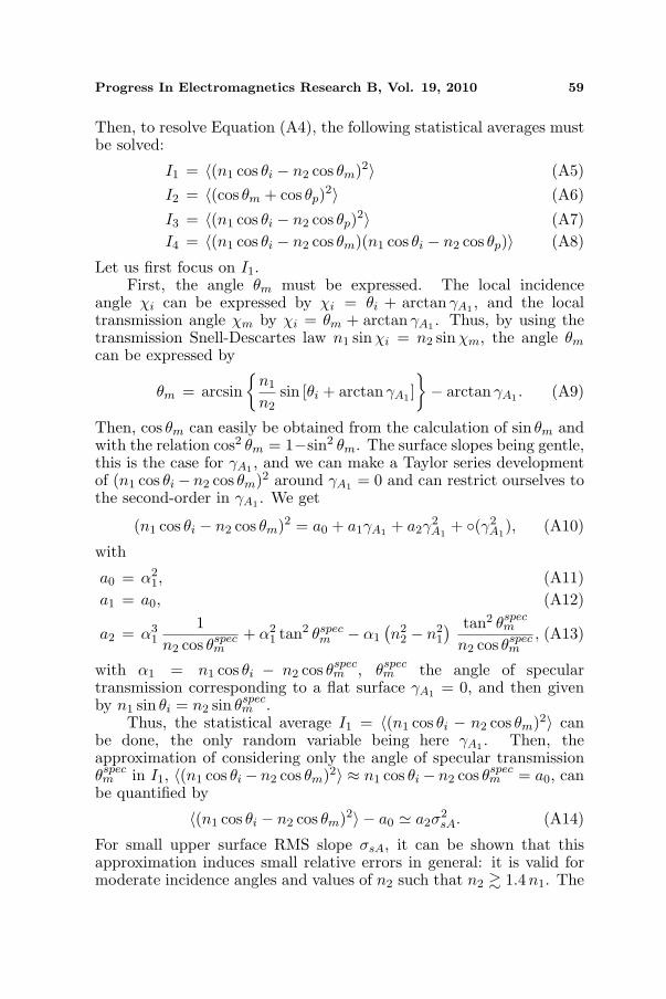
Then, to resolve Equation (A4), the following statistical averages mustbe solved:

I1 = 〈(n1 cos θi − n2 cos θm)2〉 (A5)I2 = 〈(cos θm + cos θp)2〉 (A6)

I3 = 〈(n1 cos θi − n2 cos θp)2〉 (A7)I4 = 〈(n1 cos θi − n2 cos θm)(n1 cos θi − n2 cos θp)〉 (A8)

Let us first focus on I1.First, the angle θm must be expressed. The local incidence

angle χi can be expressed by χi = θi + arctan γA1 , and the localtransmission angle χm by χi = θm + arctan γA1 . Thus, by using thetransmission Snell-Descartes law n1 sinχi = n2 sinχm, the angle θm

can be expressed by

θm = arcsin

n1

n2sin [θi + arctan γA1 ]

− arctan γA1 . (A9)

Then, cos θm can easily be obtained from the calculation of sin θm andwith the relation cos2 θm = 1−sin2 θm. The surface slopes being gentle,this is the case for γA1 , and we can make a Taylor series developmentof (n1 cos θi− n2 cos θm)2 around γA1 = 0 and can restrict ourselves tothe second-order in γA1 . We get

(n1 cos θi − n2 cos θm)2 = a0 + a1γA1 + a2γ2A1

+ (γ2A1

), (A10)

with

a0 = α21, (A11)

a1 = a0, (A12)

a2 = α31

1n2 cos θspec

m+ α2

1 tan2 θspecm − α1

(n2

2 − n21

) tan2 θspecm

n2 cos θspecm

, (A13)

with α1 = n1 cos θi − n2 cos θspecm , θspec

m the angle of speculartransmission corresponding to a flat surface γA1 = 0, and then givenby n1 sin θi = n2 sin θspec

m .Thus, the statistical average I1 = 〈(n1 cos θi − n2 cos θm)2〉 can

be done, the only random variable being here γA1 . Then, theapproximation of considering only the angle of specular transmissionθspecm in I1, 〈(n1 cos θi − n2 cos θm)2〉 ≈ n1 cos θi − n2 cos θspec

m = a0, canbe quantified by

〈(n1 cos θi − n2 cos θm)2〉 − a0 ' a2σ2sA. (A14)

For small upper surface RMS slope σsA, it can be shown that thisapproximation induces small relative errors in general: it is valid formoderate incidence angles and values of n2 such that n2 & 1.4n1. The


same developments and general conclusions can be drawn for the otherstatistical averages I2, I3, and I4.

Thus, a Taylor series development up to the second order of thefirst three terms of Equation (A4) over the random variables γA1 andγB1 can be led to check the general approximation of consideringspecular angles θspec

m and θspecp = −θspec

m in 〈(δφr,2)2〉. After statistical

average, this leads to the relation

〈(δφr,2)2〉 = b0 + b1Aσ2

sA + b1Bσ2sB, (A15)

with

b0=2k20

[(n1−n2)2σ2

hA+2n22σ

2hB

]+2k2

0

[n1

n2(n1−n2)2σ2

hA−2n21σ

2hB

]θ2i ,(A16)

b1A = 2k20(n1 − n2)2 β1, (A17)

b1B = 4k20n

22 β1, (A18)

with β1 =[

n1−n2n2

σ2hA − 2σ2

hB

]. This means that the approximation of

specular angles implies the condition

b1Aσ2sA + b1Bσ2

sB

b0¿ 1. (A19)

For small upper and lower RMS slopes σsA and σsB, respectively (ofthe order of σsA, . 0.3), it can be shown that this condition is validfor moderate incidence angles and values of n2 such that n2 & 1.4n1.

Up to now, we did not take the fourth term inside Equation (A4)into account. In fact, a similar derivation would show that thisterm does not significantly contribute for moderate incidence anglesand values of n2 such that n2 & 1.4n1. In conclusion, under theseconditions and with gentle RMS slopes (of the order of σsA, σsB .0.3), the approximation of taking specular propagation angles insidethe rough layer is valid.

ACKNOWLEDGMENT

The authors would like to thank the anonymous reviewers for theircomments that help improve the manuscript.

REFERENCES

1. Rayleigh, L., “On the dynamical theory of gratings,” Proceedingsof the Royal Society of London. Series A, Containing Papers of aMathematical and Physical Character, Vol. 79, No. 532, 399–416,Aug. 1907.


2. Rayleigh, L., The Theory of Sound, Dover, New York, 1945,(originally published in 1877).

3. Ogilvy, J., Theory of Wave Scattering from Random Surfaces,Institute of Physics Publishing, Bristol and Philadelphia, 1991.

4. Elfouhaily, T. and C.-A. Guerin, “A critical survey of approximatescattering wave theories from random rough surfaces,” Waves inRandom Media, Vol. 14, No. 4, R1–R40, 2004.

5. Ament, W., “Toward a theory of reflection by a rough surface,”IRE Proc., Vol. 41, 142–146, 1953.

6. Freund, D., N. Woods, H.-C. Ku, and R. Awadallah,“Forward radar propagation over a rough sea surface: Anumerical assessment of the Miller-Brown approximation using ahorizontally polarized 3-GHz line source,” IEEE Transactions onAntennas and Propagation, Vol. 54, No. 4, 1292–1304, Apr. 2006.

7. Yin, Z., H. S. Tan, and F. W. Smith, “Determination of theoptical constants of diamond films with a rough growth surface,”Diamonds and Related Materials, Vol. 5, No. 12, 1490–1496, 1996.

8. Yin, Z., Z. Akkerman, B. Yang, and F. Smith, “Optical propertiesand microstructure of CVD diamond films,” Diamonds andRelated Materials, Vol. 6, No. 1, 153–158, Jan. 1997.

9. Ohlidal, I. and K. Navratil, “Scattering of light from multilayerwith rough boundaries,” Progress in Optics, E. Wolf (ed.), Vol. 34,249–331, Elsevier Science, 1995.

10. Aziz, A., W. Papousek, and G. Leising, “Polychromaticreflectance and transmittance of a slab with a randomly roughboundary,” Applied Optics, Vol. 38, No. 25, 5422–5428, Sep. 1999.

11. Poruba, A., A. Fejfar, Z. Remes, J. Springer, M. Vanecek,J. Kocka, J. Meier, P. Torres, and A. Shah, “Optical absorptionand light scattering in microcrystalline silicon thin films andsolar cells,” Journal of Applied Physics, Vol. 88, No. 1, 148–160,Jul. 2000.

12. Choi, S., S. Lee, and K. H. Koh, “In situ optical investigationof carbon nanotube growth in hot-filament chemical vapordeposition,” Current Applied Physics, Vol. 6, 38–42, Aug. 2006.

13. Xiong, R., P. J. Wissmann, and M. A. Gallivan, “Anextended Kalman filter for in situ sensing of yttria-stabilizedzirconia in chemical vapor deposition,” Computers and ChemicalEngineering, Vol. 30, No. 10–12, 1657–1669, Sep. 2006.

14. Maury, F. and F.-D. Duminica, “Diagnostic in TCOs CVDprocesses by IR pyrometry,” Thin Solid Films, Vol. 515, No. 24,8619–8623, Oct. 2007.


15. Remes, Z., A. Kromka, and M. Vanecek, “Towards optical-qualitynanocrystalline diamond with reduced non-diamond content,”Physica Status Solidi A, Vol. 206, No. 9, 2004–2008, Sep. 2009.

16. Fabbro, V., C. Bourlier, and P. F. Combes, “Forward propagationmodeling above Gaussian rough surfaces by the parabolic shad-owing effect,” Progress In Electromagnetics Research, PIER 58,243–269, 2006.

17. Pinel, N., C. Bourlier, and J. Saillard, “Forward radarpropagation over oil slicks on sea surfaces using the Ament modelwith shadowing effect,” Progress In Electromagnetics Research,PIER 76, 95–126, 2007.

18. Wu, Z.-S., J.-P. Zhang, L. Guo, and P. Zhou, “An improvedtwo-scale model with volume scattering for the dynamic oceansurface,” Progress In Electromagnetics Research, PIER 89, 39–56,2009.

19. Wang, M.-J., Z.-S. Wu, and Y.-L. Li, “Investigation on thescattering characteristics of Gaussian beam from two dimensionaldielectric rough surfaces based on the Kirchhoff approximation,”Progress In Electromagnetics Research B, Vol. 4, 223–235, 2008.

20. Wang, R. and L. Guo, “Numerical simulations wave scatteringfrom two-layered rough interface,” Progress In ElectromagneticsResearch B, Vol. 10, 163–175, 2008.

21. Boithias, L., Radio Wave Propagation, McGraw-Hill, Ed., NorthOxford Academic Publishers, London, UK, 1987.

22. Landron, O., M. Feuerstein, and T. Rappaport, “A comparison oftheoretical and empirical reflection coefficients for typical exteriorwall surfaces in a mobile radio environment,” IEEE Transactionson Antennas and Propagation, Vol. 44, No. 3, 341–351, Mar. 1996.

23. Didascalou, D., M. Dottling, N. Geng, and W. Wiesbeck,“An approach to include stochastic rough surface scatteringinto deterministic ray-optical wave propagation modeling,” IEEETransactions on Antennas and Propagation, Vol. 51, No. 7, 1508–1515, Jul. 2003.

24. Jraifi, A., E. H. Saidi, A. E. Khafaji, and A. E. Rhalami,“Theoretical modelisation of rough surfaces in radio propagationchannel,” IEEE 3rd International Symposium on Image/VideoCommunications over Fixed and Mobile Networks, Tunisia,Sep. 2006.

25. Cocheril, Y. and R. Vauzelle, “A new ray-tracing based wavepropagation model including rough surfaces scattering,” ProgressIn Electromagnetics Research, PIER 75, 357–381, 2007.


26. Tsang, L. and J. Kong, Scattering of Electromagnetic Waves,Volume III: Advanced Topics, John Wiley & Sons, New York,2001.

27. Soubret, A., “Diffusion des ondes electromagnetiques par desmilieux et des surfaces aleatoires: etude des effets coherents dansle champ diffuse,” Ph.D. dissertation, Universite d’Aix-Marseille2, Marseille, France, 2001.

28. Caron, J., J. Lafait, and C. Andraud, “Scalar Kirchhoff’s modelfor light scattering from dielectric random rough surfaces,” OpticsCommunications, Vol. 207, 17–28, Jun. 2002.

29. Pinel, N., C. Bourlier, and J. Saillard, “Rayleigh parameter ofa rough layer: Application to forward radar propagation over oilslicks on sea surfaces under the Ament model,” Microwave andOptical Technology Letters, Vol. 49, No. 9, 2285–2290, Sep. 2007.

30. Beckmann, P. and A. Spizzichino, The Scattering of Electromag-netic Waves From Rough Surfaces, Pergamon Press, Oxford, 1963.

31. Ulaby, F., R. Moore, and A. Fung, Microwave Remote Sensing:Active and Passive, Advanced Book Program, Vol. 2 — RadarRemote Sensing and Surface Scattering and Emission TheoryReading, Addison-Wesley, Massachusetts, 1982.

32. Thorsos, E., “The validity of the Kirchhoff approximation forrough surface scattering using a Gaussian roughness spectrum,”J. Acoustical Soc. of America, Vol. 83, No. 1, 78–92, Jan. 1988.

33. Tsang, L., J. Kong, K. Ding, and C. Ao, Scattering ofElectromagnetic Waves, Volume I: Theories and Applications,John Wiley & Sons, New York, 2000.

34. Pinel, N. and C. Bourlier, “Scattering from very rough layersunder the geometric optics approximation: Further investigation,”Journal of the Optical Society of America A, Vol. 25, No. 6, 1293–1306, Jun. 2008.

35. Pinel, N., “Etude de modeles asymptotiques de la diffusiondes ondes electromagnetiques par des interfaces naturelles —Application a une mer recouverte de petrole,” Ph.D. dissertation,Ecole polytechnique de l’universite de Nantes, Nantes, France,Oct. 2006.

36. Roo, R. D. and C.-T. Tai, “Plane wave reflection and refractioninvolving a finitely conducting medium,” IEEE Antennas andPropagation Magazine, Vol. 45, No. 5, 54–61, Oct. 2003.

37. Saillard, M. and G. Toso, “Electromagnetic scattering frombounded or infinite subsurface bodies,” Radio Science, Vol. 32,No. 4, 1347–1360, 1997.

DEGREE OF ROUGHNESS OF ROUGH LAYERS: … · Progress In Electromagnetics Research B, Vol. 19,...

Documents

Transcript of DEGREE OF ROUGHNESS OF ROUGH LAYERS: … · Progress In Electromagnetics Research B, Vol. 19,...