3Defining computation

“there is no reason why mental as well as bodily laborshould not be economized by the aid of machinery”,Charles Babbage, 1852

“If, unwarned by my example, any man shall undertakeand shall succeed in constructing an engine embody-ing in itself the whole of the executive department ofmathematical analysis upon different principles or bysimpler mechanical means, I have no fear of leaving myreputation in his charge, for he alone will be fully able toappreciate the nature of my efforts and the value of theirresults.”, Charles Babbage, 1864

“To understand a program you must become both themachine and the program.”, Alan Perlis, 1982

People have been computing for thousands of years, with aids thatinclude not just pen and paper, but also abacus, slide rulers, variousmechanical devices, and modern electronic computers. A priori, thenotion of computation seems to be tied to the particular mechanismthat you use. You might think that the “best” algorithm for multiply-ing numbers will differ if you implement it in Python on a modernlaptop than if you use pen and paper. However, as we saw in theintroduction (Chapter 0), an algorithm that is asymptotically betterwould eventually beat a worse one regardless of the underlying tech-nology. This gives us hope for a technology independent way of definingcomputation, which is what we will do in this chapter.

Compiled on 6.30.2018 23:47

Learning Objectives:• See that computation can be precisely modeled.

• Learn the computational model of Booleancircuits / straightline programs.

• See the NAND operation and also why thespecific choice of NAND is not important.

• Examples of computing in the physical world.

• Equivalence of circuits and programs.

116 introduction to theoretical computer science

Figure 3.1: Calculating wheels by Charles Babbage. Image taken from the Mark I‘operating manual’

Figure 3.2: A 1944 Popular Mechanics article on the Harvard Mark I computer.

defining computation 117

1 Indeed, extrapolation from examplesis still the way most of us first learnalgorithms such as addition and multi-plication, see Fig. 3.4)2 Translation from “The Algebra ofBen-Musa”, Fredric Rosen, 1831.

3.1 DEFINING COMPUTATION

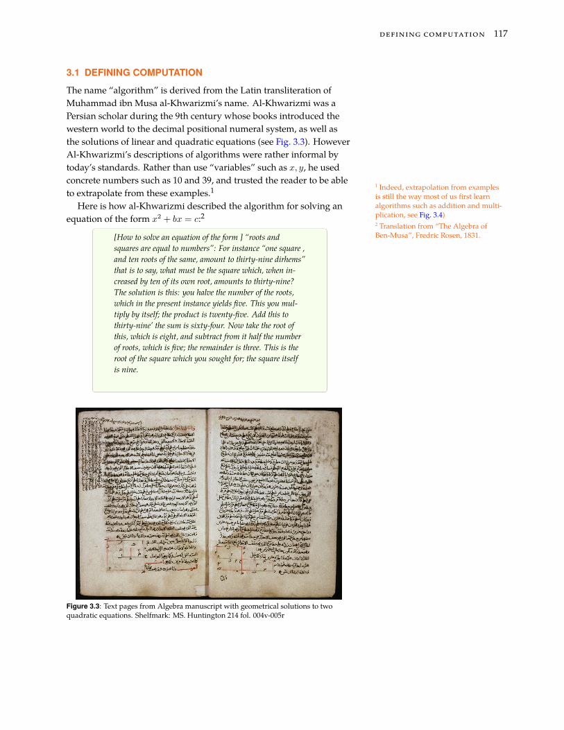
The name “algorithm” is derived from the Latin transliteration ofMuhammad ibn Musa al-Khwarizmi’s name. Al-Khwarizmi was aPersian scholar during the 9th century whose books introduced thewestern world to the decimal positional numeral system, as well asthe solutions of linear and quadratic equations (see Fig. 3.3). HoweverAl-Khwarizmi’s descriptions of algorithms were rather informal bytoday’s standards. Rather than use “variables” such as 𝑥, 𝑦, he usedconcrete numbers such as 10 and 39, and trusted the reader to be ableto extrapolate from these examples.1

Here is how al-Khwarizmi described the algorithm for solving anequation of the form 𝑥2 + 𝑏𝑥 = 𝑐:2

[How to solve an equation of the form ] “roots andsquares are equal to numbers”: For instance “one square ,and ten roots of the same, amount to thirty-nine dirhems”that is to say, what must be the square which, when in-creased by ten of its own root, amounts to thirty-nine?The solution is this: you halve the number of the roots,which in the present instance yields five. This you mul-tiply by itself; the product is twenty-five. Add this tothirty-nine’ the sum is sixty-four. Now take the root ofthis, which is eight, and subtract from it half the numberof roots, which is five; the remainder is three. This is theroot of the square which you sought for; the square itselfis nine.

Figure 3.3: Text pages from Algebra manuscript with geometrical solutions to twoquadratic equations. Shelfmark: MS. Huntington 214 fol. 004v-005r

118 introduction to theoretical computer science

Figure 3.4: An explanation for children of the two digit addition algorithm

3 As mentioned in Remark 2.1.1

For the purposes of this course, we will need a much more preciseway to describe algorithms. Fortunately (or is it unfortunately?), atleast at the moment, computers lag far behind school-age childrenin learning from examples. Hence in the 20th century people havecome up with exact formalisms for describing algorithms, namelyprogramming languages. Here is al-Khwarizmi’s quadratic equationsolving algorithm described in the Python programming language:3,this is not a programming course, and it is absolutely fine if you don’tknow Python. Still the code below should be fairly self-explanatory.]

from math import sqrt

#Pythonspeak to enable use of the sqrt function to

compute square roots.↪

def solve_eq(b,c):

# return solution of x^2 + bx = c following Al

Khwarizmi's instructions↪

# Al Kwarizmi demonstrates this for the case

b=10 and c= 39↪

val1 = b/2.0 # "halve the number of the roots"

val2 = val1*val1 # "this you multiply by itself"

val3 = val2 + c # "Add this to thirty-nine"

val4 = sqrt(val3) # "take the root of this"

defining computation 119

val5 = val4 - val1 # "subtract from it half the

number of roots"↪

return val5 # "This is the root of the square

which you sought for"↪

# Test: solve x^2 + 10*x = 39

print(solve_eq(10,39))

# 3.0

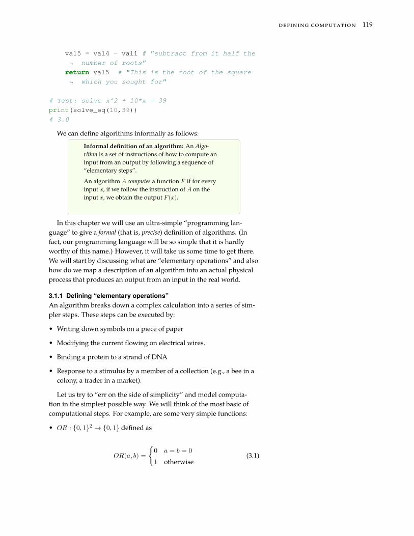
We can define algorithms informally as follows:

Informal definition of an algorithm: An Algo-rithm is a set of instructions of how to compute aninput from an output by following a sequence of“elementary steps”.

An algorithm 𝐴 computes a function 𝐹 if for everyinput 𝑥, if we follow the instruction of 𝐴 on theinput 𝑥, we obtain the output 𝐹(𝑥).

In this chapter we will use an ultra-simple “programming lan-guage” to give a formal (that is, precise) definition of algorithms. (Infact, our programming language will be so simple that it is hardlyworthy of this name.) However, it will take us some time to get there.We will start by discussing what are “elementary operations” and alsohow do we map a description of an algorithm into an actual physicalprocess that produces an output from an input in the real world.

3.1.1 Defining “elementary operations”An algorithm breaks down a complex calculation into a series of sim-pler steps. These steps can be executed by:

• Writing down symbols on a piece of paper

• Modifying the current flowing on electrical wires.

• Binding a protein to a strand of DNA

• Response to a stimulus by a member of a collection (e.g., a bee in acolony, a trader in a market).

Let us try to “err on the side of simplicity” and model computa-tion in the simplest possible way. We will think of the most basic ofcomputational steps. For example, are some very simple functions:

• 𝑂𝑅 ∶ {0, 1}2 → {0, 1} defined as

𝑂𝑅(𝑎, 𝑏) =⎧{⎨{⎩

0 𝑎 = 𝑏 = 01 otherwise

(3.1)

120 introduction to theoretical computer science

• 𝐴𝑁𝐷 ∶ {0, 1}2 → {0, 1} defined as

𝐴𝑁𝐷(𝑎, 𝑏) =⎧{⎨{⎩

1 𝑎 = 𝑏 = 10 otherwise

(3.2)

• 𝑁𝑂𝑇 ∶ {0, 1} → {0, 1} defind as 𝑁𝑂𝑇 (𝑎) = 1 − 𝑎.

Each one of these functions takes either one or two single bits asinput, and produces a single bit as output. Clearly, it cannot get muchmore basic than these. However, the power of computation comesfrom composing simple building blocks together.

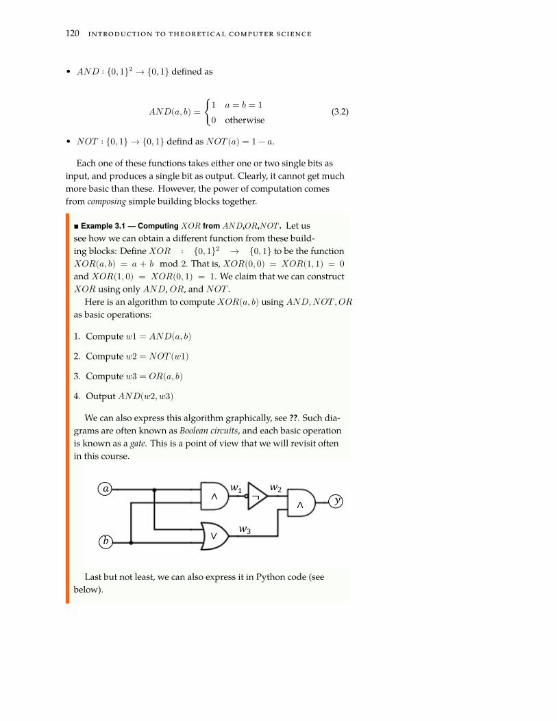
� Example 3.1 — Computing 𝑋𝑂𝑅 from 𝐴𝑁𝐷,𝑂𝑅,𝑁𝑂𝑇 . Let ussee how we can obtain a different function from these build-ing blocks: Define 𝑋𝑂𝑅 ∶ {0, 1}2 → {0, 1} to be the function𝑋𝑂𝑅(𝑎, 𝑏) = 𝑎 + 𝑏 mod 2. That is, 𝑋𝑂𝑅(0, 0) = 𝑋𝑂𝑅(1, 1) = 0and 𝑋𝑂𝑅(1, 0) = 𝑋𝑂𝑅(0, 1) = 1. We claim that we can construct𝑋𝑂𝑅 using only 𝐴𝑁𝐷, 𝑂𝑅, and 𝑁𝑂𝑇 .

Here is an algorithm to compute 𝑋𝑂𝑅(𝑎, 𝑏) using 𝐴𝑁𝐷, 𝑁𝑂𝑇 , 𝑂𝑅as basic operations:

1. Compute 𝑤1 = 𝐴𝑁𝐷(𝑎, 𝑏)

2. Compute 𝑤2 = 𝑁𝑂𝑇 (𝑤1)

3. Compute 𝑤3 = 𝑂𝑅(𝑎, 𝑏)

4. Output 𝐴𝑁𝐷(𝑤2, 𝑤3)

We can also express this algorithm graphically, see ??. Such dia-grams are often known as Boolean circuits, and each basic operationis known as a gate. This is a point of view that we will revisit oftenin this course.

Last but not least, we can also express it in Python code (seebelow).

defining computation 121

def AND(a,b): return a*b

def OR(a,b): return 1-(1-a)*(1-b)

def NOT(a): return 1-a

def XOR(a,b):

w1 = AND(a,b)

w2 = NOT(w1)

w3 = OR(a,b)

return AND(w2,w3)

print([f"XOR({a},{b})={XOR(a,b)}" for a in [0,1]

for b in [0,1]])↪

# ['XOR(0,0)=0', 'XOR(0,1)=1', 'XOR(1,0)=1',

'XOR(1,1)=0']↪

� Example 3.2 — Computing 𝑋𝑂𝑅 on three bits. Extending the sameideas, we can use these basic operations to compute the function𝑋𝑂𝑅3 ∶ {0, 1}3 → {0, 1} defined as 𝑋𝑂𝑅3(𝑎, 𝑏, 𝑐) = 𝑎 + 𝑏 + 𝑐(mod 2) by computing first 𝑑 = 𝑋𝑂𝑅(𝑎, 𝑏) and then outputting𝑋𝑂𝑅(𝑑, 𝑐). In Python this is done as follows:

def XOR3(a,b,c):

w1 = AND(a,b)

w2 = NOT(w1)

w3 = OR(a,b)

w4 = AND(w2,w3)

w5 = AND(w4,c)

w6 = NOT(w5)

w7 = OR(w4,c)

return AND(w6,w7)

print([f"XOR3({a},{b},{c})={XOR3(a,b,c)}" for a

in [0,1] for b in [0,1] for c in [0,1]])↪

# ['XOR3(0,0,0)=0', 'XOR3(0,0,1)=1',

'XOR3(0,1,0)=1', 'XOR3(0,1,1)=0',

'XOR3(1,0,0)=1', 'XOR3(1,0,1)=0',

'XOR3(1,1,0)=0', 'XOR3(1,1,1)=1']

↪

↪

↪

P Make sure you see how to generalize this and obtaina way to compute 𝑋𝑂𝑅𝑛 ∶ {0, 1}𝑛 → {0, 1} for every𝑛 using at most 4𝑛 basic steps involving applicationsof a function in {𝐴𝑁𝐷, 𝑂𝑅, 𝑁𝑂𝑇 } to omputs or

122 introduction to theoretical computer science

previously computed values.

3.1.2 The NAND functionHere is another function we can compute using 𝐴𝑁𝐷, 𝑂𝑅, 𝑁𝑂𝑇 . The𝑁𝐴𝑁𝐷 function maps {0, 1}2 to {0, 1} and is defined as

𝑁𝐴𝑁𝐷(𝑎, 𝑏) =⎧{⎨{⎩

0 𝑎 = 𝑏 = 11 otherwise

(3.3)

As its name implies, 𝑁𝐴𝑁𝐷 is the NOT of AND (i.e.,𝑁𝐴𝑁𝐷(𝑎, 𝑏) = 𝑁𝑂𝑇 (𝐴𝑁𝐷(𝑎, 𝑏))), and so we can clearly com-pute 𝑁𝐴𝑁𝐷 using 𝐴𝑁𝐷 and 𝑁𝑂𝑇 . Interestingly, the oppositedirection also holds:

Theorem 3.3 — NAND computes AND,OR,NOT.. We can compute 𝐴𝑁𝐷,𝑂𝑅, and 𝑁𝑂𝑇 by composing only the 𝑁𝐴𝑁𝐷 function.

Proof. We start with the following observation. For every 𝑎 ∈ {0, 1},𝐴𝑁𝐷(𝑎, 𝑎) = 𝑎. Hence, 𝑁𝐴𝑁𝐷(𝑎, 𝑎) = 𝑁𝑂𝑇 (𝐴𝑁𝐷(𝑎, 𝑎)) = 𝑁𝑂𝑇 (𝑎).This means that 𝑁𝐴𝑁𝐷 can compute 𝑁𝑂𝑇 , and since by the principleof “double negation”, 𝐴𝑁𝐷(𝑎, 𝑏) = 𝑁𝑂𝑇 (𝑁𝑂𝑇 (𝐴𝑁𝐷(𝑎, 𝑏))) thismeans that we can use 𝑁𝐴𝑁𝐷 to compute 𝐴𝑁𝐷 as well. Once we cancompute 𝐴𝑁𝐷 and 𝑁𝑂𝑇 , we can compute 𝑂𝑅 using the so called “DeMorgan’s Law”: 𝑂𝑅(𝑎, 𝑏) = 𝑁𝑂𝑇 (𝐴𝑁𝐷(𝑁𝑂𝑇 (𝑎), 𝑁𝑂𝑇 (𝑏))) for every𝑎, 𝑏 ∈ {0, 1}. �

P Theorem 3.3’s proof is very simple, but you shouldmake sure that (i) you understand the statement ofthe theorem, and (ii) you follow its proof completely.In particular, you should make sure you understandwhy De Morgan’s law is true.

R Verify NAND’s universality by Python (optional) Ifyou are so inclined, you can also verify the proof ofTheorem 3.3 by Python:

def NAND(a,b): return 1-a*b

def ORwithNAND(a,b):

return NAND(NAND(a,a),NAND(b,b))

print([f"Test {a},{b}:

{ORwithNAND(a,b)==OR(a,b)}" for a in

[0,1] for b in [0,1]])

↪

↪

defining computation 123

# ['Test 0,0: True', 'Test 0,1: True',

'Test 1,0: True', 'Test 1,1: True']↪

Solved Exercise 3.1 — Compute majority with NAND. Let 𝑀𝐴𝐽3 ∶{0, 1}3 → {0, 1} be the function that on input 𝑎, 𝑏, 𝑐 outputs 1 iff𝑎 + 𝑏 + 𝑐 ≥ 2. Show how to compute 𝑀𝐴𝐽3 using a composition of𝑁𝐴𝑁𝐷’s. �

Solution: To solve this problem, we will first express 𝑀𝐴𝐽3 using𝐴𝑁𝐷, 𝑂𝑅, 𝑁𝑂𝑇 , and then use Theorem 3.3 to replace those withonly 𝑁𝐴𝑁𝐷. We can very naturally express the statement “Atleast two of 𝑎, 𝑏, 𝑐 are equal to 1” using OR’s and AND’s. Specifi-cally, this is true if at least one of the values 𝐴𝑁𝐷(𝑎, 𝑏), 𝐴𝑁𝐷(𝑎, 𝑐),𝐴𝑁𝐷(𝑏, 𝑐) is true. So we can write

𝑀𝐴𝐽3(𝑎, 𝑏, 𝑐) = 𝑂𝑅(𝑂𝑅(𝐴𝑁𝐷(𝑎, 𝑏), 𝐴𝑁𝐷(𝑎, 𝑐)), 𝐴𝑁𝐷(𝑏, 𝑐)) .(3.4)

Now we can use the equivalence 𝐴𝑁𝐷(𝑎, 𝑏) = 𝑁𝑂𝑇 (𝑁𝐴𝑁𝐷(𝑎, 𝑏)),𝑂𝑅(𝑎, 𝑏) = 𝑁𝐴𝑁𝐷(𝑁𝑂𝑇 (𝑎), 𝑁𝑂𝑇 (𝑏)), and 𝑁𝑂𝑇 (𝑎) = 𝑁𝐴𝑁𝐷(𝑎, 𝑎)to replace the righthand side of Eq. (3.4) with an expression involv-ing only 𝑁𝐴𝑁𝐷, yielding

𝑀𝐴𝐽3(𝑎, 𝑏, 𝑐) = 𝑁𝐴𝑁𝐷(𝑁𝐴𝑁𝐷(𝑁𝐴𝑁𝐷(𝑁𝐴𝑁𝐷(𝑎, 𝑏), 𝑁𝐴𝑁𝐷(𝑎, 𝑐)), 𝑁𝐴𝑁𝐷(𝑁𝐴𝑁𝐷(𝑎, 𝑏), 𝑁𝐴𝑁𝐷(𝑎, 𝑐))), 𝑁𝐴𝑁𝐷(𝑏, 𝑐))(3.5)

This corresponds to the following circuit with 𝑁𝐴𝑁𝐷 gates:

124 introduction to theoretical computer science

�

3.2 INFORMALLY DEFINING “BASIC OPERATIONS” AND “AL-GORITHMS”

Theorem 3.3 tells us that we can use applications of the single function𝑁𝐴𝑁𝐷 to obtain 𝐴𝑁𝐷, 𝑂𝑅, 𝑁𝑂𝑇 , and so by extension all the otherfunctions that can be built up from them. So, if we wanted to decideon a “basic operation”, we might as well choose 𝑁𝐴𝑁𝐷, as we’llget “for free” the three other operations 𝐴𝑁𝐷, 𝑂𝑅 and 𝑁𝑂𝑇 . Thissuggests the following definition of an “algorithm”:

Semi-formal definition of an algorithm: An al-gorithm consists of a sequence of steps of the form“store the NAND of variables bar and blah invariable foo”.

An algorithm 𝐴 computes a function 𝐹 if for everyinput 𝑥 to 𝐹 , if we feed 𝑥 as input to the algorithm,the value computed in its last step is 𝐹(𝑥).

There are several concerns that are raised by this definition:

1. First and foremost, this definition is indeed too informal. We do notspecify exactly what each step does, nor what it means to “feed 𝑥 asinput”.

defining computation 125

2. Second, the choice of 𝑁𝐴𝑁𝐷 as a basic operation seems arbitrary.Why just 𝑁𝐴𝑁𝐷? Why not 𝐴𝑁𝐷, 𝑂𝑅 or 𝑁𝑂𝑇 ? Why not allowoperations like addition and multiplication? What about any otherlogical constructions such if/then or while?

3. Third, do we even know that this definition has anything to dowith actual computing? If someone gave us a description of such analgorithm, could we use it to actually compute the function the realworld?

P These concerns will to a large extent guide us in theupcoming chapters. Thus you would be well advisedto re-read the above informal definition and see whatyou think about these issues.

A large part of this course will be devoted to adressing the aboveissues. We will see that:

1. We can make the definition of an algorithm fully formal, and sogive a precise mathematical meaning to statements such as “Algo-rithm 𝐴 computes function 𝐹”.

2. While the choice of 𝑁𝐴𝑁𝐷 is arbitrary, and we could just as wellchose some other functions, we will also see this choice does notmatter much. Our notion of an algorithm is not more restrictivebecause we only think of 𝑁𝐴𝑁𝐷 as a basic step. We have alreadyseen that allowing 𝐴𝑁𝐷,𝑂𝑅, 𝑁𝑂𝑇 as basic operations will notadd any power (because we can compute them from 𝑁𝐴𝑁𝐷’svia Theorem 3.3). We will see that the same is true for addition,multiplication, and essentially every other operation that could bereasonably thought of as a basic step.

3. It turns out that we can and do compute such “𝑁𝐴𝑁𝐷 based algo-rithms” in the real world. First of all, such an algorithm is clearlywell specified, and so can be executed by a human with a pen andpaper. Second, there are a variety of ways to mechanize this compu-tation. We’ve already seen that we can write Python code that cor-responds to following such a list of instructions. But in fact we candirectly implement operations such as 𝑁𝐴𝑁𝐷, 𝐴𝑁𝐷, 𝑂𝑅, 𝑁𝑂𝑇etc.. via electronic signals using components known as transistors.This is how modern electronic computers operate.

In the remainder of this chapter, we will begin to answer some ofthese questions. We will see more example of the power of simpleoperations like 𝑁𝐴𝑁𝐷 (or equivalently, 𝐴𝑁𝐷/𝑂𝑅/𝑁𝑂𝑇 , as well asmany other choices) to compute more complex operations including

126 introduction to theoretical computer science

addition, multiplication, sorting and more. We will then discuss howto physically implement simple operations such as NAND using a va-riety of technologies. Finally we will define The NAND programminglanguage that will be our formal model of computation.

3.3 FROM NAND TO INFINITY AND BEYOND..

We have seen that using 𝑁𝐴𝑁𝐷, we can compute 𝐴𝑁𝐷, 𝑂𝑅, 𝑁𝑂𝑇and 𝑋𝑂𝑅. But this still seems a far cry from being able to add andmultiply numbers, not to mention more complex programs such assorting and searching, solving equations, manipulating images, andso on. We now give a few examples demonstrating how we can usethese simple operations to do some more complicated tasks. While wewill not go as far as implementing Call of Duty using 𝑁𝐴𝑁𝐷, we willat least show how we can compose 𝑁𝐴𝑁𝐷 operations to obtain taskssuch as addition, multiplications, and comparisons.

3.3.1 NAND CircuitsWe can describe the computation of a function 𝐹 ∶ {0, 1}𝑛 → {0, 1}via a composition of 𝑁𝐴𝑁𝐷 operations in terms of a circuit, as wasdone in ??. Since in our case, all the gates are the same function (i.e.,𝑁𝐴𝑁𝐷), the description of the circuit is even simpler. We can thinkof the circuit as a directed graph. It has a vertex for every one of theinput bits, and also for every intermediate value we use in our com-putation. If we compute a value 𝑢 by applying 𝑁𝐴𝑁𝐷 to 𝑣 and 𝑤then we put a directed edges from 𝑣 to 𝑢 and from 𝑤 to 𝑢. We will fol-low the convention of using “𝑥” for inputs and “𝑦” for outputs, andhence write 𝑥0, 𝑥1, … for our inputs and 𝑦0, 𝑦1, … for our outputs. (Wewill sometimes also write these as X[0],X[1],… and Y[0],Y[1],…respectively.) Here is a more formal definition:

P Before reading the formal definition, it would bean extremely good exercise for you to pause hereand try to think how you would formally define thenotion of a NAND circuit. Sometimes working outthe definition for yourself is easier than parsing itstext.

Definition 3.4 — NAND circuits. Let 𝑛, 𝑚, 𝑠 > 0. A NAND circuit 𝐶with 𝑛 inputs, 𝑚 outputs, and 𝑠 gates is a labeled directed acyclicgraph (DAG) with 𝑛 + 𝑠 vertices such that:

• 𝐶 has 𝑛 vertices with no incoming edges, which are called theinput vertices and are labeled with X[0],…, X[𝑛 − 1].

defining computation 127

• 𝐶 has 𝑠 vertices each with exactly two (possibly parallel) incom-ing edges, which are called the gates.

• 𝐶 has 𝑚 gates which are called the output vertices and are la-beled with Y[0],…,Y[𝑚 − 1]. The output vertices have nooutgoing edges.

For 𝑥 ∈ {0, 1}𝑛, the output of 𝐶 on input 𝑥, denoted by 𝐶(𝑋), iscomputed in the natural way. For every 𝑖 ∈ [𝑛], we assign to theinput vertex X[𝑖] the value 𝑥𝑖, and then continuously assign toevery gate the value which is the NAND of the values assigned toits two incoming neighbors. The output is the string 𝑦 ∈ {0, 1}𝑚

such that for every 𝑗 ∈ [𝑚], 𝑦𝑗 is the value assigned to the outputgate labeled with Y[𝑗].

P Definition 3.4 is perhaps our first encounter witha somewhat complicated definition. When youare faced with such a definition, there are severalstrategies to try to understand it:

1. First, as we suggested above, you might want tosee how you would formalize the intuitive notionthat the definitions tries to capture. If we madedifferent choices than you would, try to think whyis that the case.

2. Then, you should read the definition carefully,making sure you understand all the terms that ituses, and all the conditions it imposes.

3. Finally, try to how the definition correspondsto simple examples such as the NAND circuitpresented in Eq. (3.4), as well as the examplesillustrated below.

We now present some examples of 𝑁𝐴𝑁𝐷 circuits for variousnatural problems:

� Example 3.5 — 𝑁𝐴𝑁𝐷 circuit for 𝑋𝑂𝑅. Recall the 𝑋𝑂𝑅 functionwhich maps 𝑥0, 𝑥1 ∈ {0, 1} to 𝑥0 + 𝑥1 mod 2. We have seen inExample 3.1 that we can compute this function using 𝐴𝑁𝐷, 𝑂𝑅,and 𝑁𝑂𝑇 , and so by Theorem 3.3 we can compute it using only𝑁𝐴𝑁𝐷’s. However, the following is a direct construction of com-puting 𝑋𝑂𝑅 by a sequence of NAND operations:

1. Let 𝑢 = 𝑁𝐴𝑁𝐷(𝑥0, 𝑥1).

2. Let 𝑣 = 𝑁𝐴𝑁𝐷(𝑥0, 𝑢)

128 introduction to theoretical computer science

3. Let 𝑤 = 𝑁𝐴𝑁𝐷(𝑥1, 𝑢).

4. The 𝑋𝑂𝑅 of 𝑥0 and 𝑥1 is 𝑦0 = 𝑁𝐴𝑁𝐷(𝑣, 𝑤).

(We leave it to you to verify that this algorithm does indeedcompute 𝑋𝑂𝑅.)

We can also represent this algorithm graphically as a circuit:

We now present a few more examples of computing natural func-tions by a sequence of 𝑁𝐴𝑁𝐷 operations.

� Example 3.6 — 𝑁𝐴𝑁𝐷 circuit for incrementing. Consider the taskof computing, given as input a string 𝑥 ∈ {0, 1}𝑛 that representsa natural number 𝑋 ∈ ℕ, the representation of 𝑋 + 1. That is,we want to compute the function 𝐼𝑁𝐶𝑛 ∶ {0, 1}𝑛 → {0, 1}𝑛+1

such that for every 𝑥0, … , 𝑥𝑛−1, 𝐼𝑁𝐶𝑛(𝑥) = 𝑦 which satisfies∑𝑛

𝑖=0 𝑦𝑖2𝑖 = (∑𝑛−1𝑖=0 𝑥𝑖2𝑖) + 1.

The increment operation can be very informally described asfollows: “Add 1 to the least significant bit and propagate the carry”. Alittle more precisely, in the case of the binary representation, toobtain the increment of 𝑥, we scan 𝑥 from the least significant bitonwards, and flip all 1’s to 0’s until we encounter a bit equal to 0, inwhich case we flip it to 1 and stop. (Please verify you understandwhy this is the case.)

Thus we can compute the increment of 𝑥0, … , 𝑥𝑛−1 by doing the

defining computation 129

following:

1. Set 𝑐0 = 1 (we pretend we have a “carry” of 1 initially)

2. For 𝑖 = 0, … , 𝑛 − 1 do the following:

1. Let 𝑦𝑖 = 𝑋𝑂𝑅(𝑥𝑖, 𝑐𝑖).

2. If 𝑦𝑖 = 𝑥𝑖 = 1 then 𝑐𝑖+1 = 1, else 𝑐𝑖+1 = 0.

1. Set 𝑦𝑛 = 𝑐𝑛.

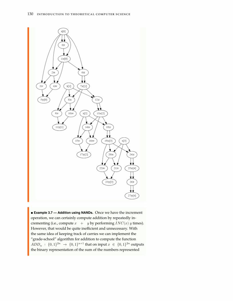
The above is a very precise description of an algorithm to com-pute the increment operation, and can be easily transformed intoPython code that performs the same computation, but it does notseem to directly yield a NAND circuit to compute this. However,we can transform this algorithm line by line to a NAND circuit. Forexample, since for every 𝑎, 𝑁𝐴𝑁𝐷(𝑎, 𝑁𝑂𝑇 (𝑎)) = 1, we can replacethe initial statement 𝑐0 = 1 with 𝑐0 = 𝑁𝐴𝑁𝐷(𝑥0, 𝑁𝐴𝑁𝐷(𝑥0, 𝑥0)).We already know how to compute 𝑋𝑂𝑅 using NAND, so line 2.acan be replaced by some NAND operations. Next, we can writeline 2.b as simply saying 𝑐𝑖+1 = 𝐴𝑁𝐷(𝑦𝑖, 𝑥𝑖), or in other words𝑐𝑖+1 = 𝑁𝐴𝑁𝐷(𝑁𝐴𝑁𝐷(𝑦𝑖, 𝑥𝑖), 𝑁𝐴𝑁𝐷(𝑦𝑖, 𝑥𝑖)). Finally, the assign-ment 𝑦𝑛 = 𝑐𝑛 can be written as 𝑦𝑛 = 𝑁𝐴𝑁𝐷(𝑁𝐴𝑁𝐷(𝑐𝑛, 𝑐𝑛), 𝑁𝐴𝑁𝐷(𝑐𝑛, 𝑐𝑛)).Combining these observations yields for every 𝑛 ∈ ℕ, a 𝑁𝐴𝑁𝐷 cir-cuit to compute 𝐼𝑁𝐶𝑛. For example, this is how this circuit lookslike for 𝑛 = 4.

130 introduction to theoretical computer science

� Example 3.7 — Addition using NANDs. Once we have the incrementoperation, we can certainly compute addition by repeatedly in-crementing (i.e., compute 𝑥 + 𝑦 by performing 𝐼𝑁𝐶(𝑥) 𝑦 times).However, that would be quite inefficient and unnecessary. Withthe same idea of keeping track of carries we can implement the“grade-school” algorithm for addition to compute the function𝐴𝐷𝐷𝑛 ∶ {0, 1}2𝑛 → {0, 1}𝑛+1 that on input 𝑥 ∈ {0, 1}2𝑛 outputsthe binary representation of the sum of the numbers represented

defining computation 131

by 𝑥0, … , 𝑥𝑛−1 and 𝑥𝑛+1, … , 𝑥𝑛:

1. Set 𝑐0 = 0.

2. For 𝑖 = 0, … , 𝑛 − 1:

1. Let 𝑦𝑖 = 𝑥𝑖 + 𝑥𝑛+𝑖 + 𝑐𝑖( mod 2).

2. If 𝑥𝑖 + 𝑥𝑛+𝑖 + 𝑐𝑖 ≥ 2 then 𝑐𝑖+1 = 1.

1. Let 𝑦𝑛 = 𝑐𝑛

Once again, this can be translated into a NAND circuit. To trans-form Step 2.b to a NAND circuit we use the fact (shown in SolvedExercise 3.1) that the function 𝑀𝐴𝐽3 ∶ {0, 1}3 → {0, 1} can becomputed using 𝑁𝐴𝑁𝐷s.

3.4 PHYSICAL IMPLEMENTATIONS OF COMPUTING DEVICES.

Computation is an abstract notion, that is distinct from its physicalimplementations. While most modern computing devices are obtainedby mapping logical gates to semi-conductor based transistors, overhistory people have computed using a huge variety of mechanisms,including mechanical systems, gas and liquid (known as fluidics),biological and chemical processes, and even living creatures (e.g., seeFig. 3.5 or this video for how crabs or slime mold can be used to docomputations).

In this section we will review some of these implementations, bothso you can get an appreciation of how it is possible to directly trans-late NAND programs to the physical world, without going throughthe entire stack of architecture, operating systems, compilers, etc… aswell as to emphasize that silicon-based processors are by no means theonly way to perform computation. Indeed, as we will see much laterin this course, a very exciting recent line of works involves using dif-ferent media for computation that would allow us to take advantageof quantum mechanical effects to enable different types of algorithms.

3.4.1 Transistors and physical logic gatesA transistor can be thought of as an electric circuit with two inputs,known as source and gate and an output, known as the sink. The gatecontrols whether current flows from the source to the sink. In a stan-dard transistor, if the gate is “ON” then current can flow from thesource to the sink and if it is “OFF” then it can’t. In a complementarytransistor this is reversed: if the gate is “OFF” then current can flowfrom the source to the sink and if it is “ON” then it can’t.

There are several ways to implement the logic of a transistor. Forexample, we can use faucets to implement it using water pressure

132 introduction to theoretical computer science

Figure 3.5: Crab-based logic gates from the paper “Robust soldier-crab ball gate” byGunji, Nishiyama and Adamatzky. This is an example of an AND gate that relies onthe tendency of two swarms of crabs arriving from different directions to combine to asingle swarm that continues in the average of the directions.

Figure 3.6: We can implement the logic of transistors using water. The water pressurefrom the gate closes or opens a faucet between the source and the sink.

defining computation 133

4 This might seem as curiosity but thereis a field known as fluidics concernedwith implementing logical operationsusing liquids or gasses. Some of the mo-tivations include operating in extremeenvironmental conditions such as inspace or a battlefield, where standardelectronic equipment would not survive.

(e.g. Fig. 3.6).4 However, the standard implementation uses electricalcurrent. One of the original implementations used vacuum tubes. Asits name implies, a vacuum tube is a tube containing nothing (i.e.,vacuum) and where a priori electrons could freely flow from source(a wire) to the sink (a plate). However, there is a gate (a grid) betweenthe two, where modulating its voltage can block the flow of electrons.

Early vacuum tubes were roughly the size of lightbulbs (and lookedvery much like them too). In the 1950’s they were supplanted by tran-sistors, which implement the same logic using semiconductors whichare materials that normally do not conduct electricity but whoseconductivity can be modified and controlled by inserting impuri-ties (“doping”) and an external electric field (this is known as the fieldeffect). In the 1960’s computers were started to be implemented usingintegrated circuits which enabled much greater density. In 1965, Gor-don Moore predicted that the number of transistors per circuit woulddouble every year (see Fig. 3.7), and that this would lead to “suchwonders as home computers —or at least terminals connected to acentral computer— automatic controls for automobiles, and personalportable communications equipment”. Since then, (adjusted versionsof) this so-called “Moore’s law” has been running strong, thoughexponential growth cannot be sustained forever, and some physicallimitations are already becoming apparent.

Figure 3.7: The number of transistors per integrated circuits from 1959 till 1965 and aprediction that exponential growth will continue at least another decade. Figure takenfrom “Cramming More Components onto Integrated Circuits”, Gordon Moore, 1965

134 introduction to theoretical computer science

Figure 3.8: Gordon Moore’s cartoon “predicting” the implications of radically improv-ing transistor density.

Figure 3.9: The exponential growth in computing power over the last 120 years. Graphby Steve Jurvetson, extending a prior graph of Ray Kurzweil.

defining computation 135

3.4.2 NAND gates from transistorsWe can use transistors to implement a NAND gate, which would be asystem with two input wires 𝑥, 𝑦 and one output wire 𝑧, such that ifwe identify high voltage with “1” and low voltage with “0”, then thewire 𝑧 will equal to “1” if and only if the NAND of the values of thewires 𝑥 and 𝑦 is 1 (see Fig. 3.10).

Figure 3.10: Implementing a NAND gate using transistors.

This means that there exists a NAND circuit to compute a function𝐹 ∶ {0, 1}𝑛 → {0, 1}𝑚, then we can compute 𝐹 in the physical worldusing transistors as well.

3.5 BASING COMPUTING ON OTHER MEDIA (OPTIONAL)

Electronic transistors are in no way the only technology that can im-plement computation. There are many mechanical, chemical, bio-logical, or even social systems that can be thought of as computingdevices. We now discuss some of these examples.

3.5.1 Biological computingComputation can be based on biological or chemical systems. For ex-ample the lac operon produces the enzymes needed to digest lactoseonly if the conditions 𝑥 ∧ (¬𝑦) hold where 𝑥 is “lactose is present” and𝑦 is “glucose is present”. Researchers have managed to create transis-tors, and from them the NAND function and other logic gates, basedon DNA molecules (see also Fig. 3.11). One motivation for DNA com-puting is to achieve increased parallelism or storage density; another

136 introduction to theoretical computer science

is to create “smart biological agents” that could perhaps be injectedinto bodies, replicate themselves, and fix or kill cells that were dam-aged by a disease such as cancer. Computing in biological systems isnot restricted of course to DNA. Even larger systems such as flocks ofbirds can be considered as computational processes.

Figure 3.11: Performance of DNA-based logic gates. Figure taken from paper of Bonnetet al, Science, 2013.

3.5.2 Cellular automata and the game of lifeCellular automata is a model of a system composed of a sequence ofcells, which of which can have a finite state. At each step, a cell up-dates its state based on the states of its neighboring cells and somesimple rules. As we will discuss later in this course, cellular automatasuch as Conway’s “Game of Life” can be used to simulate computa-tion gates, see Fig. 3.12.

3.5.3 Neural networksOne computation device that we all carry with us is our own brain.Brains have served humanity throughout history, doing computationsthat range from distinguishing prey from predators, through makingscientific discoveries and artistic masterpieces, to composing witty280 character messages. The exact working of the brain is still notfully understood, but it seems that to a first approximation it can bemodeled by a (very large) neural network.

A neural network is a Boolean circuit that instead of 𝑁𝐴𝑁𝐷 (or

defining computation 137

Figure 3.12: An AND gate using a “Game of Life” configuration. Figure taken fromJean-Philippe Rennard’s paper.

5 Threshold is just one example of gatesthat can used by neural networks.More generally, a neural network isoften described as operating on signalsthat are real numbers, rather than 0/1values, and where the output of a gateon inputs 𝑥0, … , 𝑥𝑘−1 is obtained byapplying 𝑓(∑𝑖 𝑤𝑖𝑥𝑖) where 𝑓 ∶ ℝ → ℝis an an activation function such asrectified linear unit (ReLU), Sigmoid, ormany others. However, for the purposeof our discussion, all of the aboveare equivalent. In particular we canreduce the real case to the binary caseby a real number in the binary basis,and multiplying the weight of the bitcorresponding to the 𝑖𝑡ℎ digit by 2𝑖.

even 𝐴𝑁𝐷/𝑂𝑅/𝑁𝑂𝑇 ) uses some other gates as the basic basis. Forexample, ine particular basis we can use are threshold gates. For everyvector 𝑤 = (𝑤0, … , 𝑤𝑘−1) of integers and integer 𝑡 (some or all ofwhom could be negative), the threshold function corresponding to 𝑤, 𝑡is the function 𝑇𝑤,𝑡 ∶ {0, 1}𝑘 → {0, 1} that maps 𝑥 ∈ {0, 1}𝑘 to 1 ifand only if ∑𝑘−1

𝑖=0 𝑤𝑖𝑥𝑖 ≥ 𝑡. For example, the threshold function 𝑇𝑤,𝑡corresponding to 𝑤 = (1, 1, 1, 1, 1) and 𝑡 = 3 is simply the majorityfunction 𝑀𝐴𝐽5 on {0, 1}5. The function 𝑁𝐴𝑁𝐷 ∶ {0, 1}2 → {0, 1} isthe threshold function corresponding to 𝑤 = (−1, −1) and 𝑡 = −1,since 𝑁𝐴𝑁𝐷(𝑥0, 𝑥1) = 1 if and only if 𝑥0 + 𝑥1 ≤ 1 or equivalently,−𝑥0 − 𝑥1 ≥ −1.5

Threshold gates can be thought of as an approximation for neuroncells that make up the core of human and animal brains. To a firstapproximation, a neuron has 𝑘 inputs and a single output and theneurons “fires” or “turns on” its output when those signals pass somethreshold. Unlike the cases above, when we considered the numberof inputs to a gate 𝑘 to be a small constant, in such neural networkswe often do not put any bound on the number of inputs. However,since any threshold function on 𝑘 inputs can be computed by a NANDcircuit of at most 𝑝𝑜𝑙𝑦(𝑘) gates (see Exercise 3.3), NAND circuits are noless powerful than neural networks.

3.5.4 The marble computerTO BE COMPLETED

3.6 THE NAND PROGRAMMING LANGUAGE

We now turn to formally defining the notion of algorithm. We usea programming language to do so. We define the NAND Programming

138 introduction to theoretical computer science

6 We follow the common program-ming languages convention of usingnames such as foo, bar, baz, blah asstand-ins for generic identifiers. Gener-ally a variable identifier in the NANDprogramming language can be anycombination of letters and numbers, andwe will also sometimes have identifierssuch as Foo[12] that end with a num-ber inside square brackets. Later in thecourse we will introduce programminglanguages where such identifiers carryspecial meaning as arrays. At the mo-ment you can treat them as simply anyother identifier. The appendix containsa full formal specification of the NANDprogramming language.

Language to be a programming language where every line has thefollowing form:

foo = NAND(bar,blah)

where foo, bar and blah are variable identifiers.6

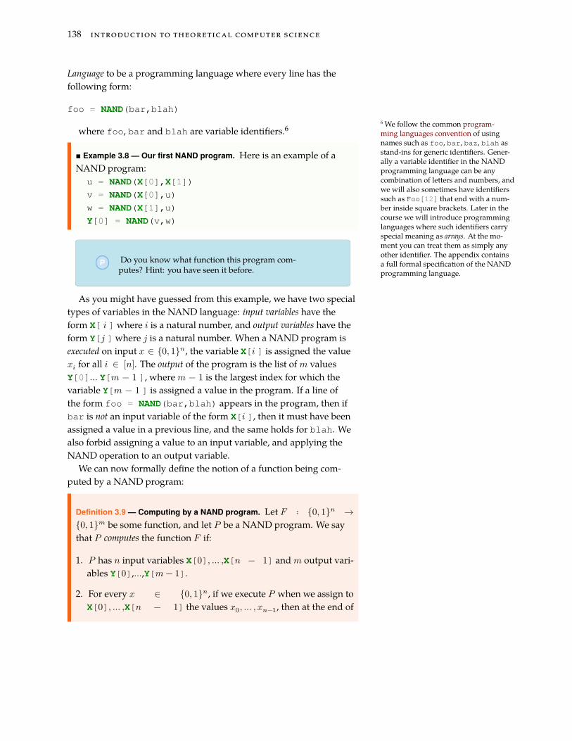
� Example 3.8 — Our first NAND program. Here is an example of aNAND program:

u = NAND(X[0],X[1])

v = NAND(X[0],u)

w = NAND(X[1],u)

Y[0] = NAND(v,w)

P Do you know what function this program com-putes? Hint: you have seen it before.

As you might have guessed from this example, we have two specialtypes of variables in the NAND language: input variables have theform X[ 𝑖 ] where 𝑖 is a natural number, and output variables have theform Y[𝑗 ] where 𝑗 is a natural number. When a NAND program isexecuted on input 𝑥 ∈ {0, 1}𝑛, the variable X[𝑖 ] is assigned the value𝑥𝑖 for all 𝑖 ∈ [𝑛]. The output of the program is the list of 𝑚 valuesY[0]… Y[𝑚 − 1 ], where 𝑚 − 1 is the largest index for which thevariable Y[𝑚 − 1 ] is assigned a value in the program. If a line ofthe form foo = NAND(bar,blah) appears in the program, then ifbar is not an input variable of the form X[𝑖 ], then it must have beenassigned a value in a previous line, and the same holds for blah. Wealso forbid assigning a value to an input variable, and applying theNAND operation to an output variable.

We can now formally define the notion of a function being com-puted by a NAND program:

Definition 3.9 — Computing by a NAND program. Let 𝐹 ∶ {0, 1}𝑛 →{0, 1}𝑚 be some function, and let 𝑃 be a NAND program. We saythat 𝑃 computes the function 𝐹 if:

1. 𝑃 has 𝑛 input variables X[0], … ,X[𝑛 − 1] and 𝑚 output vari-ables Y[0],…,Y[𝑚 − 1].

2. For every 𝑥 ∈ {0, 1}𝑛, if we execute 𝑃 when we assign toX[0], … ,X[𝑛 − 1] the values 𝑥0, … , 𝑥𝑛−1, then at the end of

defining computation 139

the execution, the output variables Y[0],…,Y[𝑚 − 1] have thevalues 𝑦0, … , 𝑦𝑚−1.

P Definition 3.9 is one of the most important defini-tions in this book. Please make sure to read it timeand again until you are sure that you understand it.A full formal specification of the execution model ofNAND programs appears in the appendix.

R Is the NAND programming language Turing Com-plete? (optional note) You might have heard of aterm called “Turing Complete” to describe program-ming languages. (If you haven’t, feel free to ignorethe rest of this remark: we will encounter this termlater in this course and define it properly.) If so, youmight wonder if the NAND programming languagehas this property. The answer is no, or perhaps moreaccurately, the term is not really applicable for theNAND programming language. The reason is that,by design, the NAND programming language canonly compute finite functions 𝐹 ∶ {0, 1}𝑛 → {0, 1}𝑚

that take a fixed number of input bits and producea fixed number of outputs bits. The term “TuringComplete” is really only applicable to program-ming languages for infinite functions that can takeinputs of arbitrary length. We will come back to thisdistinction later on in the course.

3.6.1 NAND programs and NAND circuitsSo far we have described two models of computation:

• NAND circuits, which are obtained by applying NAND gates toinputs.

• NAND programs, which are obtained by repeatedly applying opera-tions of the form foo = NAND(bar,blah).

A central result is that these two models are actually equivalent:

Theorem 3.10 — Circuit and straightline program equivalence. Let𝐹 ∶ {0, 1}𝑛 → {0, 1}𝑚 and 𝑠 ∈ ℕ. Then 𝐹 is computable by a NANDprogram of 𝑠 lines if and only if it is computable by a NAND circuitof 𝑠 gates.

Proof Idea: To understand the proof, you can first work out for yourselfthe equivalence between the NAND program of Example 3.8 and

140 introduction to theoretical computer science

the circuit we have seen in Example 3.5, see also Fig. 3.13. Generally,if we have a NAND program, we can transform it into a circuit bymapping every line foo = NAND(bar,blah) of the program intoa gate foo that is applied to the result of the previous gates bar andblah. (Since we always assign a variable to variables that have beenassigned before or are input variables, we can assume that bar andblah are either gates we already constructed or are inputs to thecircuit.) In the reverse direction, to map a circuit 𝐶 into a program 𝑃we use topological sorting to sort the vertices of the graph of 𝐶 intoan order 𝑣0, 𝑣1, … , 𝑣𝑠−1 such that if there is an edge from 𝑣𝑖 to 𝑣𝑗 then𝑗 > 𝑖. Thus we can transform every gate (i.e. non input vertex) of thecircuit into a line in a program in an analogous way: if 𝑣 is a gate thathas two incoming edges from 𝑢 and 𝑤, then we add a variable foocorresonding to 𝑣 and a line foo = NAND(bar,blah) where barand blah are the variables corresponding to 𝑢 and 𝑤. ⋆

Figure 3.13: The NAND code and the corresponding circuit for a program to computethe increment function that maps a string 𝑥 ∈ {0, 1}3 (which we think of as a number in[7]) to the string 𝑦 ∈ {0, 1}4 that represents 𝑥 + 1. Note how every line in the programcorresponds to a gate in the circuit.

Proof of Theorem 3.10. Let 𝐹 ∶ {0, 1}𝑛 → {0, 1}𝑚 be a function. Supposethat there exists a program 𝑃 of 𝑠 lines that computes 𝐹 . We constructa NAND circuit 𝐶 to compute 𝐹 as follows: the circuit will include𝑛 input vertices, and will include 𝑠 gates, one for each of the lines of𝑃 . We let 𝐼(0), … , 𝐼(𝑛 − 1) denotes the vertices corresponding to theinputs and 𝐺(0), … , 𝐺(𝑠 − 1) denote the vertices corresponding to thelines. We connect our gates in the natural way as follows:

If the ℓ-th line of 𝑃 has the form foo = NAND(bar,blah) wherebar and blah are variables not of the form X[𝑖], then bar and blah

defining computation 141

must have been assigned a value before. We let 𝑗 and 𝑘 be the last linesbefore the ℓ-th line in which the variables bar and blah respectivelywere assigned a value. In such a case, we will add the edges ⃗⃗⃗ ⃗⃗ ⃗⃗ ⃗⃗ ⃗⃗ ⃗⃗ ⃗⃗ ⃗⃗ ⃗⃗ ⃗⃗ ⃗⃗ ⃗⃗ ⃗⃗ ⃗⃗ ⃗⃗ ⃗⃗ ⃗⃗ ⃗𝐺(𝑗) 𝐺(ℓ)and ⃗⃗⃗⃗⃗⃗⃗⃗⃗ ⃗⃗⃗⃗⃗⃗⃗⃗⃗⃗⃗⃗⃗⃗⃗⃗⃗⃗⃗⃗⃗⃗⃗⃗⃗⃗⃗𝐺(𝑘) 𝐺(ℓ) to our circuit 𝐶. That is, we will apply the gate 𝐺(ℓ) tothe outputs of the gates 𝐺(𝑗) and 𝐺(𝑘). If bar is an input variable ofthe form X[𝑖] then we connect 𝐺(ℓ) to the corresponding input vertex𝐼(𝑖), and do the analogous step if blah is an input variable. Finally,for every 𝑗 ∈ [𝑚], if ℓ(𝑗) is the last line which assigns a value to Y[𝑗],then we mark the gate 𝐺(𝑗) as the 𝑗-th output gate of the circuit 𝐶.

We claim that the circuit 𝐶 computes the same function as the pro-gram 𝑃 . Indeed, one can show by induction on ℓ that for every input𝑥 ∈ {0, 1}𝑛, if we execute 𝑃 on input 𝑥, then the value assigned tothe variable in the ℓ-th line is the same as the value output by the gate𝐺(ℓ) in the circuit 𝐶. (To see this note that by the induction hypoth-esis, this is true for the values that the ℓ-th line uses, as they wereassigned a value in earlier lines or are inputs, and both the gate andthe line compute the NAND function on these values.) Hence in par-ticular the output variables of the program will have the same value asthe output gates of the circuits.

In the other direction, given a circuit 𝐶 of 𝑠 gates that computes 𝐹 ,we can construct a program of 𝑠 lines that computes the same func-tion. We use a topological sort to ensure that the 𝑛 + 𝑠 vertices of thegraph of 𝐶 are sorted so that all edges go from earlier vertices to laterones, and ensure the first 𝑛 vertices 0, 1, … , 𝑛 − 1 correspond to the𝑛 inputs. (This can be ensured as input vertices have no incomingedges.) Then for every ℓ ∈ [𝑠], the ℓ-th line of the program 𝑃 will cor-respond to the vertex 𝑛 + ℓ of the circuit. If vertex 𝑛 + ℓ’s incomingneighbors are 𝑗 and 𝑘, then the ℓ-th line will be of the form Temp[ℓ]= NAND(Temp[𝑗 − 𝑛],Temp[𝑘 − 𝑛]) (if 𝑗 and/or 𝑘 are one of thefirst 𝑛 vertices, then we will use the corresponding input variable X[𝑗]and/or X[𝑗] instead). If vertex 𝑛 + ℓ is the 𝑗-th output gate, then weuse Y[𝑗] as the variable on the righthand side of the ℓ-th line. Onceagain by a similar inductive proof we can show that the program 𝑃 weconstructed computes the same function as the circuit 𝐶. �

R Constructive proof The proof of Theorem 3.10 isconstructive, in the sense that it yield an explicit trans-formation from a program to a circuit and vice versa.The appendix contains code of a Python function thatoutputs the circuit corresponding to a program.

R Circuits with other gate sets (advanced note) Thereis nothing special about NAND. For every set of

142 introduction to theoretical computer science

functions 𝒢 = {𝐺0, … , 𝐺𝑘−1}, we can define a no-tion of circuits that use elements of 𝒢 as gates, anda notion of a “𝒢 programming language” whereevery line involves assigning to a variable foothe result of applying some 𝐺𝑖 ∈ 𝒢 to previouslydefined or input variables. We can use the sameproof idea of Theorem 3.10 to show that 𝒢 circuitsand 𝒢 programs are equivalent. We have seen thatfor 𝒢 = {𝐴𝑁𝐷, 𝑂𝑅, 𝑁𝑂𝑇 }, the resulting circuit-s/programs are equivalent in power to the NANDprogramming language, as we can compute 𝑁𝐴𝑁𝐷using 𝐴𝑁𝐷/𝑂𝑅/𝑁𝑂𝑇 and vice versa. This turnsout to be a special case of a general phenomena- theuniversality of 𝑁𝐴𝑁𝐷 and other gate sets- that wewill explore more in depth later in this course.

✓ Lecture Recap

• An algorithm is a recipe for performing a compu-tation as a sequence of “elementary” or “simple”operations.

• One candidate definition for an “elementary” op-eration is the 𝑁𝐴𝑁𝐷 operation. It is an operationthat is easily implementable in the physical worldin a variety of methods including by electronictransistors.

• We can use 𝑁𝐴𝑁𝐷 to compute many other func-tions, including majority, increment, and others.

• There are other equivalent choices, including theset {𝐴𝑁𝐷, 𝑂𝑅, 𝑁𝑂𝑇 }.

• We can formally define the notion of a function𝐹 ∶ {0, 1}𝑛 → {0, 1}𝑚 being computable using theNAND Programming language.

• The notions of being computable by a 𝑁𝐴𝑁𝐷 cir-cuit and being computable by a 𝑁𝐴𝑁𝐷 programare equivalent.

3.7 EXERCISES

R Disclaimer Most of the exercises have been writtenin the summer of 2018 and haven’t yet been fullydebugged. While I would prefer people do not postonline solutions to the exercises, I would greatlyappreciate if you let me know of any bugs. You cando so by posting a GitHub issue about the exercise,and optionally complement this with an email to mewith more details about the attempted solution.

defining computation 143

7 Thanks to Alec Sun for solving thisproblem.

8 TODO: check the right bound, andgive it as a challenge program. Also saythe conditions under which this can beimproved to 𝑂(𝑘) or �̃�(𝑘).

Exercise 3.1 — Universal basis. Define a set 𝒢 of functions to be a uni-versal basis if we can compute 𝑁𝐴𝑁𝐷 using 𝒢. For every one of thefollowing sets, either prove that it is a universal basis or prove that it isnot. 1. 𝐵 = {∧, ∨, ¬}. (To make all of them be function on two inputs,define ¬(𝑥, 𝑦) = 𝑥.)

2. 𝐵 = {∧, ∨}.3. 𝐵 = {⊕, 0, 1} where ⊕ ∶ {0, 1}2 → {0, 1} is the XOR function and

0 and 1 are the constant functions that output 0 and 1.4. 𝐵 = {𝐿𝑂𝑂𝐾𝑈𝑃1, 0, 1} where 0 and 1 are the constant functions

as above and 𝐿𝑂𝑂𝐾𝑈𝑃1 ∶ {0, 1}3 → {0, 1} satisfies 𝐿𝑂𝑂𝐾𝑈𝑃1(𝑎, 𝑏, 𝑐)equals 𝑎 if 𝑐 = 0 and equals 𝑏 if 𝑐 = 1. �

Exercise 3.2 — Bound on universal basis size (challenge). Prove that forevery subset 𝐵 of the functions from {0, 1}𝑘 to {0, 1}, if 𝐵 is universalthen there is a 𝐵-circuit of at most 𝑂(𝑘) gates to compute the 𝑁𝐴𝑁𝐷function (you can start by showing that there is a 𝐵 circuit of at most𝑂(𝑘16) gates).7 �

Exercise 3.3 — Threshold using NANDs. Prove that for every 𝑤, 𝑡, thefunction 𝑇𝑤,𝑡 can be computed by a NAND program of at most 𝑂(𝑘3)lines.8 �

3.8 BIOGRAPHICAL NOTES

3.9 FURTHER EXPLORATIONS

Some topics related to this chapter that might be accessible to ad-vanced students include:

• Efficient constructions of circuits: finding circuits of minimal sizethat compute certain functions.

TBC