On the computation of the defining polynomial of the algebraic Riccati

equation

Yamaguchi Univ. Takuya Kitamoto

Cybernet Systems, Co. LTD Tetsu Yamaguchi

Outline of the presentation

• What is ARE (Algebraic Riccati Equation)?

• Properties of ARE

• Problem formulation

• Algorithm description

• Numerical experiments

• Conclusion

What is ARE (Algebraic Riccati Equation)?

0

such that matrix Find

symmetric) :, ( ,, matrices Given

:matrix ofEquation

QPWPPAPA

Pnn

QWQWAnn

T

4908.03646.0

3646.08554.0

10

01 ,

20

02 ,

11

10

:Example

P

QWA

Properties of ARE

• Important equation for control theory (H2 optimal control, etc)

• Symmetric solutions (solution matrices are symmetric) are important.

• There are 2^n symmetric solutions.• When matrices A, W, Q are numerical matrices,

a numerical algorithm to compute the solutions is already known.

• The numerical algorithm can not be applied when matrices A, W, Q contain a parameter.

Problem formulation

0 such that Find

10

01 ,

20

02 ,

11

1Given

QPWPPAPAP

QWk

A

T

012222

022

012222

22,22,2

22,12,1

2,22,12,22,11,12,12,11,1

22,12,1

21,11,1

2,22,1

2,11,1

pppp

pppppkppp

pppkp

pp

ppP

Example:

133)(

,16484)( ,484)(

,402488)( ,201244)(

0)()()()()(

) ordering (term basisGroebner Computing

230

231

22

233

234

02,212

2,223

2,234

2,24

2,22,11,1

kkkkf

kkkkfkkkf

kkkkfkkkkf

kfpkfpkfpkfpkf

kppp

We can compute the defining polynomial of entries of P, not P itself.

The method with Groebner Basis:

Effective for only small degree n (n=2),

because of its heavy numerical complexities

0

satisfying matrix

of entries of polynomial defining thefind

,parameter ain entries polynomialwith

symmetric) :, ( ,, matrices Given

QPWPPAPA

P

k

QWQWAnn

T

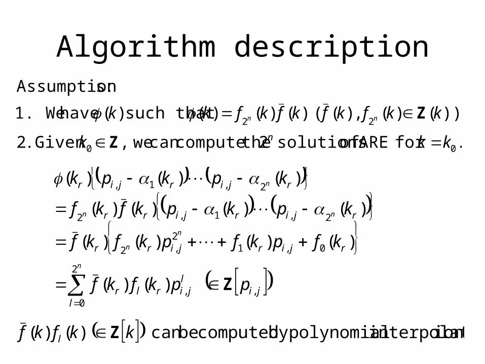
Algorithm description

.for ARE of solutions 2 thecomputecan we,Given .2

))()(, )(( )()()(such that )( have We1.

:sAssumption

00

22

kkk

kkfkfkfkfkkn

nn

Z

Z

jil

jirl

lr

rjirjirr

rjirjirr

rjirjir

ppkfkf

kfpkfpkfkf

kpkpkfkf

kpkpk

n

n

n

nn

n

,,

2

0

0,12,2

2,1,2

2,1,

)()(

)()()()(

)()()()(

)()()(

Z

ionsinterpolat polynomialby computed becan )()( kkfkf l Z

ARE of polynomial defining the

)()()()()()( 0,12,2

2

0, kfpkfpkfkfpkfkf jiji

l

ljil

n

n

n

ionsinterpolat polynomialby computed becan )()( kkfkf l Z

Algorithm

it. factorize and ionsinterpolat polynomial

by , )()( Compute 3.

)()(

)()()(

computeThen

y.numericall when ARE of )(,),(

solution thecompute andinteger an be Let .2

.)( Compute .1

,,

2

0

,,

2

0

2,1,

21

kppkfkf

ppkfkf

kpkpk

kkkk

k

kk

jilji

ll

jiljir

llr

rjirjir

r

r

n

n

n

n

Z

Z

Z

06421.03256.0

3256.02614.0 ,

0642.13256.1

3256.12614.0

,4908.16354.0

6354.08554.0 ,

4908.03646.0

3646.08554.0

.0 when ARE of

solution symmetric 42 compute and 0Let .2

1

21

kk

k

Example

10

01 ,

20

02 ,

11

1Given QW

kA

)52()1(256)( .1 26 kkkk

64102425625601280

0.640.10240.2560.25600.1280

)06421.0)(0642.1)(4908.1)(4908.0)(0(

22222

322

422

22222

322

422

22222222

pppp

pppp

pppp

64)0()0( ,1024)0()0(

256)0()0( ,2560)0()0( ,1280)0()0(

31

234

ffff

ffffff

8192)1()1( ,32768)1()1(

32768)1()1( ,131072)1()1( ,65536)1()1(

31

234

ffff

ffffff

1For 2 kk

8192327683276813107265536 22222

322

422 pppp

)14()1(64)()(

)43()1(256)()(

)1(256)()(

)52()1(512)()(

)52()1(256)()(

5,5,4,4,3,3,2,2,1,0 .3

260

261

72

263

264

kkkkfkf

kkkkfkf

kkfkf

kkkkfkf

kkkkfkf

k

1443414

528524)1(64)()(

222

2222

322

2422

264

0

kkpkkpk

pkkpkkkkfkfl

l

Conversion from floating point numbers to integers

64102425625601280

0.640.10240.2560.25600.1280

)06421.0)(0642.1)(4908.1)(4908.0)(0(

22222

322

422

22222

322

422

22222222

pppp

pppp

pppp

• Arbitrary precision arithmetic can be used.

• Precision required is unknown.

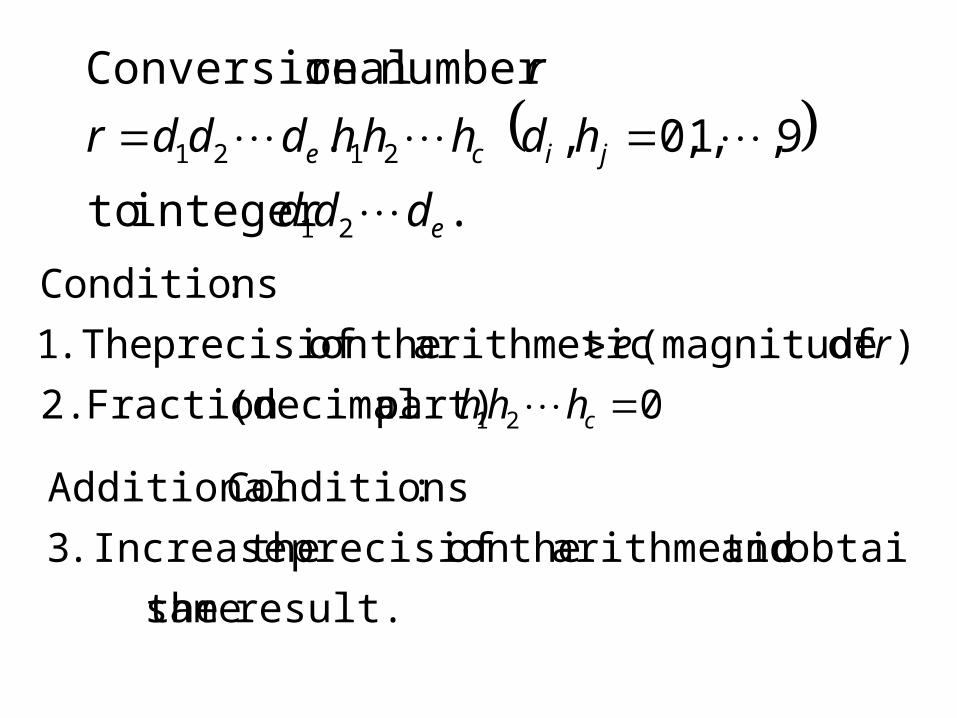
.integer to

9,,1,0, .

number real Conversion

21

2121

e

jice

ddd

hdhhhdddr

r

0 part) (decimalFraction 2.

) of (magnitude arithmetic theofprecision The .1

:Conditions

21

chhh

re

result. same the

obtain and arithmetic theofprecision theIncrease .3

:Conditions Additional

Conversion from integers to polynomials

• Polynomial interpolation can be used.

• The degree of the polynomial is unknown.

kkfkflkfkf lrlr ZZ )()(,2,1 )()(

01)(

polynomial to

,,2,1 )(

integers from Conversion

apakakg

qrkg

pp

r

Z

),,2,1( )()( .1

:Conditions

miiqq

)2()1( have Then we

.,,2,1 )( integers with edinterpolat

polynomial theof degree thebe )(Let

ppp

qrkgq

q

r

.polynomial defining theof candidate thefrom

obtained ones ith thesolution w thecompareThen

. when ARE ofsolution the

compute and integers generatedrandomly be Let .2

:Conditions Additional

0

0

kk

k

polynomial defining theof Candidate

)()()()(

)()(

0,12,2

,

2

0

kfpkfpkfkf

pkfkf

jiji

lji

ll

n

n

n

Computation of 　　　)(k

)()()(

)()()(

)()()(

),,(

matrixcertain a of

seigenvalue are ,,

),,()(

theorycontrolin AREfor algorithm numerical theFrom

21

22212

12111

11

1111

1

nnnn

n

n

n

n

jjiiji

nn

s

yvyvyv

yvyvyv

yvyvyv

yy

ss

ssk

l

).( compute toused be

canion interpolat polynomial and arithmeticpoint Floating

k

Numerical experiments (1)

5. and 5-between integer generatedrandomly :

, , ,

BEQBBW

k

A T

1

0 ,

10

01 ,

10

00 ,

21

332

2for exampleAn

BQWk

A

n

Numerical experiments (2)

paper. in this method The (M2)

basis.Groebner using method The (M1)

Environments:

Maple 10 on the machine with

Pentium M 2.0GHz, 1.5Gbyte memory

n 2 3 4 5

M10.88

4× × ×

M22.04

416.7

1766.

6×

Computation time (in seconds)

Conclusion

• An algorithm to compute the defining polynomial of ARE with a parameter is given.

• The algorithm uses polynomial interpolations and arbitrary precision arithmetic.

• Numerical experiments suggest that the algorithm is practical for the system with size n<5.

• The algorithm is suitable for multi-CPU environments.

Future direction

• Further improvements of efficiency is necessary.

• Modular algorithm instead of floating point arithmetic can be used (provided the head coefficient is known).

• Extend application of the defining polynomial.